
Parallel Computer Architecture and Programming CMU 15-418/15-618, Spring 2015
Lecture 25:
Spark (leveraging bulk-granularity program structure)

CMU 15-418/618, Spring 2015
Yeah Yeah Yeahs Sacrilege
(Mosquito)
Tunes
“In-memory performance and fault-tolerance across a cluster. No way!” - Karen O

CMU 15-418/618, Spring 2015
Analyzing site clicks 15418Log.txt
CMU 15-418/618, Spring 2015
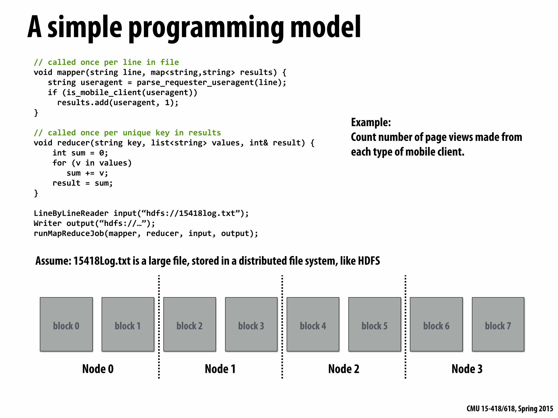
A simple programming model
Node 0 Node 1 Node 2 Node 3
Assume: 15418Log.txt is a large file, stored in a distributed file system, like HDFS
// called once per line in file void mapper(string line, map<string,string> results) { string useragent = parse_requester_useragent(line); if (is_mobile_client(useragent)) results.add(useragent, 1); }
// called once per unique key in results void reducer(string key, list<string> values, int& result) { int sum = 0; for (v in values) sum += v; result = sum; }
LineByLineReader input(“hdfs://15418log.txt”); Writer output(“hdfs://…”); runMapReduceJob(mapper, reducer, input, output);
Example: Count number of page views made from each type of mobile client.
block 0 block 1 block 2 block 3 block 4 block 5 block 6 block 7

CMU 15-418/618, Spring 2015
Let’s design an implementation of runMapReduceJob

CMU 15-418/618, Spring 2015
Step 1: running the mapper function
Node 0
15418log.txt block 0
Disk
CPU
// called once per line in file void mapper(string line, map<string,string> results) { string useragent = parse_requester_useragent(line); if (is_mobile_client(useragent)) results.add(useragent, 1); }
// called once per unique key in results void reducer(string key, list<string> values, int& result) { int sum = 0; for (v in values) sum += v; result = sum; }
LineByLineReader input(“hdfs://15418log.txt”); Writer output(“hdfs://…”); runMapReduceJob(mapper, reducer, input, output);
15418log.txt block 1
Node 1
15418log.txt block 2
Disk
CPU
15418log.txt block 3
Node 2
15418log.txt block 4
Disk
CPU
15418log.txt block 5
Node 3
15418log.txt block 6
Disk
CPU
15418log.txt block 7
Step 1: run mapper function on all lines of file Question: How to assign work to nodes?
Idea 2: data distribution based assignment: Each node processes lines in blocks of input file that are stored locally.
Idea 1: use work queue for list of input blocks to process Dynamic assignment: free node takes next available block
block 0block 1block 2
…. . .

CMU 15-418/618, Spring 2015
Steps 2 and 3: Gathering data, running the reducer
Node 0
15418log.txt block 0
Disk
CPU
// called once per line in file void mapper(string line, map<string,string> results) { string useragent = parse_requester_useragent(line); if (is_mobile_client(useragent)) results.add(useragent, 1); }
// called once per unique key in results void reducer(string key, list<string> values, int& result) { int sum = 0; for (v in values) sum += v; result = sum; }
LineByLineReader input(“hdfs://15418log.txt”); Writer output(“hdfs://…”); runMapReduceJob(mapper, reducer, input, output);
15418log.txt block 1
Step 2: Prepare intermediate data for reducer. Step 3: Run reducer function on all keys. Question: how to assign reducer tasks? Question: how to get all data for key onto the correct worker node?
Node 1
15418log.txt block 2
Disk
CPU
15418log.txt block 3
Node 2
15418log.txt block 4
Disk
CPU
15418log.txt block 5
Node 3
15418log.txt block 6
Disk
CPU
15418log.txt block 7
Safari iOSChrome
Safari iWatch
…
Keys to reduce: (generated by mapper):
Chrome Glass
Safari iOS values 0
Chrome values 0
Safari iOS values 1
Chrome values 1
Safari iOS values 2
Chrome values 2
Safari iOS values 3
Chrome values 3
Safari iWatch values 3
Chrome Glass values 0

CMU 15-418/618, Spring 2015
Node 0
15418log.txt block 0
Disk
CPU
// gather all input data for key, then execute reducer // to produce final result void runReducer(string key, reducer, result) { list<string> inputs; for (n in nodes) { filename = get_filename(key, n); read lines of filename, append into inputs; } reducer(key, inputs, result); }
15418log.txt block 1
Step 2: Prepare intermediate data for reducer. Step 3: Run reducer function on all keys. Question: how to assign reducer tasks? Question: how to get all data for key onto the correct worker node?
Node 1
15418log.txt block 2
Disk
CPU
15418log.txt block 3
Node 2
15418log.txt block 4
Disk
CPU
15418log.txt block 5
Node 3
15418log.txt block 6
Disk
CPU
15418log.txt block 7
Safari iOSChrome
Safari iWatch
…
Keys to reduce: (generated by mapper):
Chrome Glass
Safari iOS values 0
Chrome values 0
Safari iOS values 1
Chrome values 1
Safari iOS values 2
Chrome values 2
Safari iOS values 3
Chrome values 3
Safari iWatch values 3
Chrome Glass values 0
Example: Assign Safari iOS to Node 0
Steps 2 and 3: Gathering data, running the reducer

CMU 15-418/618, Spring 2015
Additional implementation challenges at scale
Node 0
15418log.txt block …
Disk15418log.txt
block …
CPU
Node 1
15418log.txt block …
Disk15418log.txt
block …
CPU
Node 2
15418log.txt block …
Disk15418log.txt
block …
CPU
Node 3
15418log.txt block …
Disk15418log.txt
block …
CPU
Node 4
15418log.txt block …
Disk15418log.txt
block …
CPU
Node 5
15418log.txt block …
Disk15418log.txt
block …
CPU
Node 6
15418log.txt block …
Disk15418log.txt
block …
CPU
Node 7
15418log.txt block …
Disk15418log.txt
block …
CPU
Node 8
15418log.txt block …
Disk15418log.txt
block …
CPU
Node 9
15418log.txt block …
Disk15418log.txt
block …
CPU
Node 10
15418log.txt block …
Disk15418log.txt
block …
CPU
Node 11
15418log.txt block …
Disk15418log.txt
block …
CPU
Node 996
15418log.txt block …
Disk15418log.txt
block …
CPU
Node 997
15418log.txt block …
Disk15418log.txt
block …
CPU
Node 998
15418log.txt block …
Disk15418log.txt
block …
CPU
Node 999
15418log.txt block …
Disk15418log.txt
block …
CPU
. . .
Node failures during program execution
Slow running nodes
CMU 15-418/618, Spring 2015
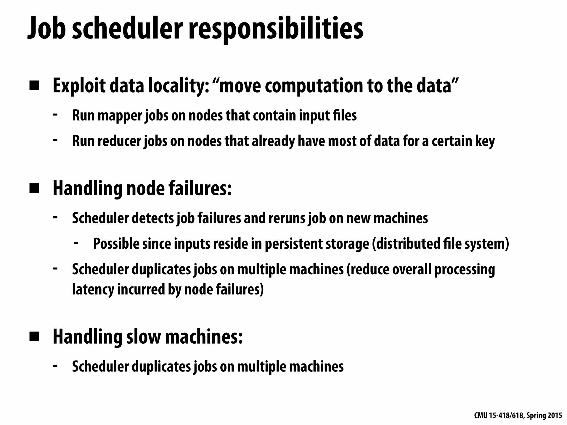
Job scheduler responsibilities
▪ Exploit data locality: “move computation to the data” - Run mapper jobs on nodes that contain input files - Run reducer jobs on nodes that already have most of data for a certain key
▪ Handling node failures: - Scheduler detects job failures and reruns job on new machines
- Possible since inputs reside in persistent storage (distributed file system) - Scheduler duplicates jobs on multiple machines (reduce overall processing
latency incurred by node failures)
▪ Handling slow machines: - Scheduler duplicates jobs on multiple machines
CMU 15-418/618, Spring 2015
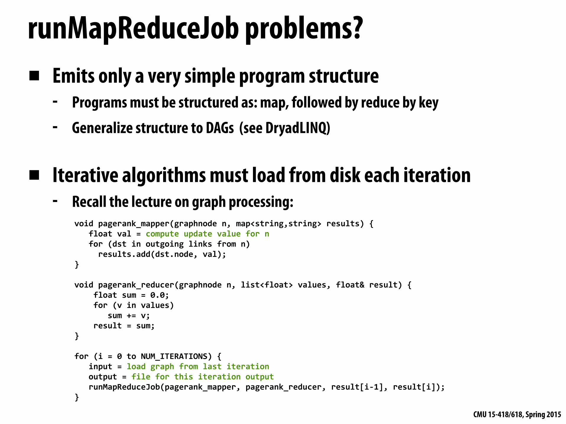
runMapReduceJob problems?▪ Emits only a very simple program structure
- Programs must be structured as: map, followed by reduce by key - Generalize structure to DAGs (see DryadLINQ)
▪ Iterative algorithms must load from disk each iteration - Recall the lecture on graph processing:
void pagerank_mapper(graphnode n, map<string,string> results) { float val = compute update value for n for (dst in outgoing links from n) results.add(dst.node, val); }
void pagerank_reducer(graphnode n, list<float> values, float& result) { float sum = 0.0; for (v in values) sum += v; result = sum; }
for (i = 0 to NUM_ITERATIONS) { input = load graph from last iteration output = file for this iteration output runMapReduceJob(pagerank_mapper, pagerank_reducer, result[i-‐1], result[i]); }
CMU 15-418/618, Spring 2015
in-memory, fault-tolerant distributed computing
CMU 15-418/618, Spring 2015
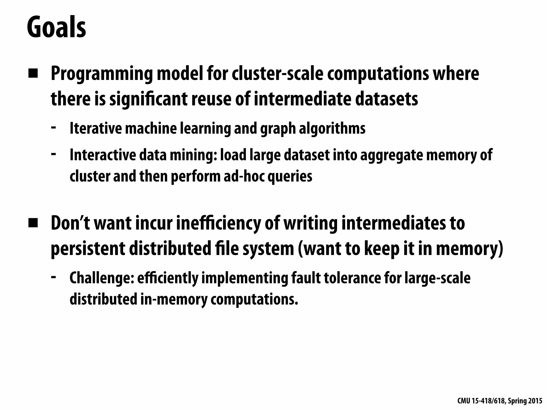
Goals▪ Programming model for cluster-scale computations where
there is significant reuse of intermediate datasets - Iterative machine learning and graph algorithms - Interactive data mining: load large dataset into aggregate memory of
cluster and then perform ad-hoc queries
▪ Don’t want incur inefficiency of writing intermediates to persistent distributed file system (want to keep it in memory) - Challenge: efficiently implementing fault tolerance for large-scale
distributed in-memory computations.

CMU 15-418/618, Spring 2015
Fault tolerance for in-memory calculations ▪ Replicate all computations
- Expensive solution: decreases peak throughput
▪ Checkpoint and rollback - Periodically save state of program to persistent storage - Restart from last checkpoint on node failure
▪ Maintain log of updates (commands and data) - High overhead for maintaining logs
Recall Map-reduce solutions: - Checkpoints after each map/reduce step by writing results to file system - Scheduler’s list of outstanding (but not yet complete) jobs is a log - Functional structure of programs allows for restart at granularity of a single
mapper or reducer invocation (don’t have to restart entire program)

CMU 15-418/618, Spring 2015
Resilient distributed dataset (RDD)Spark’s key programming abstraction:
- Read-only collection of records (immutable) - RDDs can only be created by deterministic transformations on data in
persistent storage or on existing RDDs - Actions on RDDs return data to application
// create RDD from file system data var lines = spark.textFile(“hdfs://15418log.txt”);
// create RDD using filter() transformation on lines var mobileViews = lines.filter((x: String) => isMobileClient(x));
// instruct Spark runtime to try to keep mobileViews in memory mobileViews.persist();
// create a new RDD by filtering mobileViews // then count number of elements in new RDD via count() action var numViews = mobileViews.filter(_.contains(“Safari”)).count();
// 1. create new RDD by filtering only Chrome views // 2. for each element, split string and take first element (forming new RDD) // 3. convert RDD To a scalar sequence (collect() action) var ip = mobileView.filter(_.contains(“Chrome”)) .map(_.split(“ ”)(0)) .collect();

CMU 15-418/618, Spring 2015
Repeating the map-reduce example// create RDD from file system data var lines = spark.textFile(“hdfs://15418log.txt”);
// 1. create RDD with only lines from mobile clients // 2. create RDD with elements of type (String,Int) from line string // 3. group elements by key // 4. call provided reduction function on all keys to count views var perAgentCounts = lines.filter(x => isMobileClient(x)) .map(x => (parseUserAgent(x),1)); .reduceByKey((x,y) => x+y) .collect();

CMU 15-418/618, Spring 2015
Transformations
map( f : T ) U) : RDD[T] ) RDD[U]filter( f : T ) Bool) : RDD[T] ) RDD[T]
flatMap( f : T ) Seq[U]) : RDD[T] ) RDD[U]sample(fraction : Float) : RDD[T] ) RDD[T] (Deterministic sampling)
groupByKey() : RDD[(K, V)] ) RDD[(K, Seq[V])]reduceByKey( f : (V,V)) V) : RDD[(K, V)] ) RDD[(K, V)]
union() : (RDD[T],RDD[T])) RDD[T]join() : (RDD[(K, V)],RDD[(K, W)])) RDD[(K, (V, W))]
cogroup() : (RDD[(K, V)],RDD[(K, W)])) RDD[(K, (Seq[V], Seq[W]))]crossProduct() : (RDD[T],RDD[U])) RDD[(T, U)]
mapValues( f : V ) W) : RDD[(K, V)] ) RDD[(K, W)] (Preserves partitioning)sort(c : Comparator[K]) : RDD[(K, V)] ) RDD[(K, V)]
partitionBy(p : Partitioner[K]) : RDD[(K, V)] ) RDD[(K, V)]
Actions
count() : RDD[T] ) Longcollect() : RDD[T] ) Seq[T]
reduce( f : (T,T)) T) : RDD[T] ) Tlookup(k : K) : RDD[(K, V)] ) Seq[V] (On hash/range partitioned RDDs)
save(path : String) : Outputs RDD to a storage system, e.g., HDFS
Table 2: Transformations and actions available on RDDs in Spark. Seq[T] denotes a sequence of elements of type T.
that searches for a hyperplane w that best separates twosets of points (e.g., spam and non-spam emails). The al-gorithm uses gradient descent: it starts w at a randomvalue, and on each iteration, it sums a function of w overthe data to move w in a direction that improves it.
val points = spark.textFile(...).map(parsePoint).persist()
var w = // random initial vectorfor (i <- 1 to ITERATIONS) {val gradient = points.map{ p =>p.x * (1/(1+exp(-p.y*(w dot p.x)))-1)*p.y
}.reduce((a,b) => a+b)w -= gradient
}
We start by defining a persistent RDD called pointsas the result of a map transformation on a text file thatparses each line of text into a Point object. We then re-peatedly run map and reduce on points to compute thegradient at each step by summing a function of the cur-rent w. Keeping points in memory across iterations canyield a 20⇥ speedup, as we show in Section 6.1.
3.2.2 PageRankA more complex pattern of data sharing occurs inPageRank [6]. The algorithm iteratively updates a rankfor each document by adding up contributions from doc-uments that link to it. On each iteration, each documentsends a contribution of r
n to its neighbors, where r is itsrank and n is its number of neighbors. It then updatesits rank to a/N + (1 � a)Âci, where the sum is overthe contributions it received and N is the total number ofdocuments. We can write PageRank in Spark as follows:
// Load graph as an RDD of (URL, outlinks) pairs
ranks0 input file map
contribs0
ranks1
contribs1
ranks2
contribs2
links join
reduce + map
. . .
Figure 3: Lineage graph for datasets in PageRank.
val links = spark.textFile(...).map(...).persist()var ranks = // RDD of (URL, rank) pairsfor (i <- 1 to ITERATIONS) {// Build an RDD of (targetURL, float) pairs// with the contributions sent by each pageval contribs = links.join(ranks).flatMap {(url, (links, rank)) =>links.map(dest => (dest, rank/links.size))
}// Sum contributions by URL and get new ranksranks = contribs.reduceByKey((x,y) => x+y)
.mapValues(sum => a/N + (1-a)*sum)}
This program leads to the RDD lineage graph in Fig-ure 3. On each iteration, we create a new ranks datasetbased on the contribs and ranks from the previous iter-ation and the static links dataset.6 One interesting fea-ture of this graph is that it grows longer with the number
6Note that although RDDs are immutable, the variables ranks andcontribs in the program point to different RDDs on each iteration.
RDD Transformations and ActionsTransformations: (data parallel operators taking an input RDD to a new RDD)
Actions: (provide data back to driver application)

CMU 15-418/618, Spring 2015
RDDs are distributed objects▪ Implementation of RDDs…
- May distribute contents of an RDD across nodes - May materialize RDD’s contents in memory (or disk)
// create RDD from file system data var lines = spark.textFile(“hdfs://15418log.txt”);
// create RDD using filter() transformation on lines var mobileViews = lines.filter(x => isMobileClient(x));
Node 0
15418log.txt block 0
Disk
CPU
15418log.txt block 1
DRAMmobileViews
part 1mobileViews
part 0
Node 1
15418log.txt block 2
Disk
CPU
15418log.txt block 3
DRAMmobileViews
part 3mobileViews
part 2
Node 2
15418log.txt block 4
Disk
CPU
15418log.txt block 5
DRAMmobileViews
part 5mobileViews
part 4
Node 3
15418log.txt block 6
Disk
CPU
15418log.txt block 7
DRAMmobileViews
part 7mobileViews
part 6
This example: loading RDD from storage yields one partition per filesystem block. RDD created by filter() takes on same partitions as source.

CMU 15-418/618, Spring 2015
Implementing resilience via lineage ▪ RDD transformations are, bulk, deterministic, and functional
- Implication: runtime can always reconstruct contents of RDD from its lineage (the sequence of transformations used to create it)
- Lineage is a log of transformations - Efficient: since log records bulk data-parallel operations, overhead of logging is
low (compared to logging fine-grained operations, like in a database)
// create RDD from file system data var lines = spark.textFile(“hdfs://15418log.txt”);
// create RDD using filter() transformation on lines var mobileViews = lines.filter((x: String) => isMobileClient(x));
// 1. create new RDD by filtering only Chrome views // 2. for each element, split string and take ip (first element) // 3. convert RDD To a scalar sequence (collect() action) var ip = mobileView.filter(_.contains(“Chrome”)) .map(_.split(“ ”)(0));
lines
mobileViews
Chrome views
ip
.map(_.split(“ ”)(0))
.filter(...)
.filter(...)
.load(…)

CMU 15-418/618, Spring 2015
var lines = spark.textFile(“hdfs://15418log.txt”); var mobileViews = lines.filter((x: String) => isMobileClient(x)); var ip = mobileView.filter(_.contains(“Chrome”)) .map(_.split(“ ”)(0));
Upon failure: recompute RDD partitions from lineage
Node 0
15418log.txt block 0
Disk15418log.txt
block 1
DRAM
mobileViews part 1
mobileViews part 0
Node 1
15418log.txt block 2
Disk15418log.txt
block 3
mobileViews part 3
mobileViews part 2
Node 2
15418log.txt block 4
Disk15418log.txt
block 5
mobileViews part 5
mobileViews part 4
Node 3
15418log.txt block 6
Disk15418log.txt
block 7
mobileViews part 7
mobileViews part 6
ip part 1
CPU
ip part 0
DRAMip
part 3
CPU
ip part 2
DRAMip addr part 5
CPU
ip part 4
DRAMip
part 7
CPU
ip part 6
lines
mobileViews
Chrome views
ip
.map(_.split(“ ”)(0))
.filter(...)
.filter(...)
.load(…)
Must reload required subset of data from disk and recompute entire sequence of operations given by lineage to regenerate partitions 2 and 3 of RDD ip.
Note: (not shown): file system data is replicated so assume blocks 2 and 3 remain accessible to all nodes

CMU 15-418/618, Spring 2015
var lines = spark.textFile(“hdfs://15418log.txt”); var mobileViews = lines.filter((x: String) => isMobileClient(x)); var ip = mobileView.filter(_.contains(“Chrome”)) .map(_.split(“ ”)(0));
Upon failure: recompute RDD partitions from lineage
Node 0
15418log.txt block 0
Disk15418log.txt
block 1
DRAM
mobileViews part 1
mobileViews part 0
Node 1
15418log.txt block 2
Disk15418log.txt
block 3
mobileViews part 3
mobileViews part 2
Node 2
15418log.txt block 4
Disk15418log.txt
block 5
mobileViews part 5
mobileViews part 4
Node 3
15418log.txt block 6
Disk15418log.txt
block 7
mobileViews part 7
mobileViews part 6
ip part 1
CPU
ip part 0
DRAMip
part 3
CPU
ip part 2
DRAMip addr part 5
CPU
ip part 4
DRAMip
part 7
CPU
ip part 6
lines
mobileViews
Chrome views
ip
.map(_.split(“ ”)(0))
.filter(...)
.filter(...)
.load(…)
Must reload required subset of data from disk and recompute entire sequence of operations given by lineage to regenerate partitions 2 and 3 of RDD ip.
ip part 2
ip part 3
Note: (not shown): file system data is replicated so assume blocks 2 and 3 remain accessible to all nodes

CMU 15-418/618, Spring 2015
RDD implementation▪ Internal interface for RDD objects
partitions()
preferredLocations(p)
dependencies()
iterator(p, parentIters)
partitioner()
Return a list of partitions in the RDD
Given partition p, return nodes that can access p efficiently due to locality (e.g., node that held associated block on disk, node that computed p)
List of parent RDDs
Iterator for all elements in a partition p. Requires iterators to parent RDD iterators in order to source input data
Return information about partitioning function being used. (e.g., range partitioner, hash partitioner)
Example: implementing iterator.next() for map(func) RDD transformation: void next() { return func(parentIter().next()) }
CMU 15-418/618, Spring 2015
Partitioning and dependencies
Node 0 Node 1 Node 2 Node 3
block 0 block 1 block 2 block 3 block 4 block 5 block 6 block 7
.load()
lines part 0
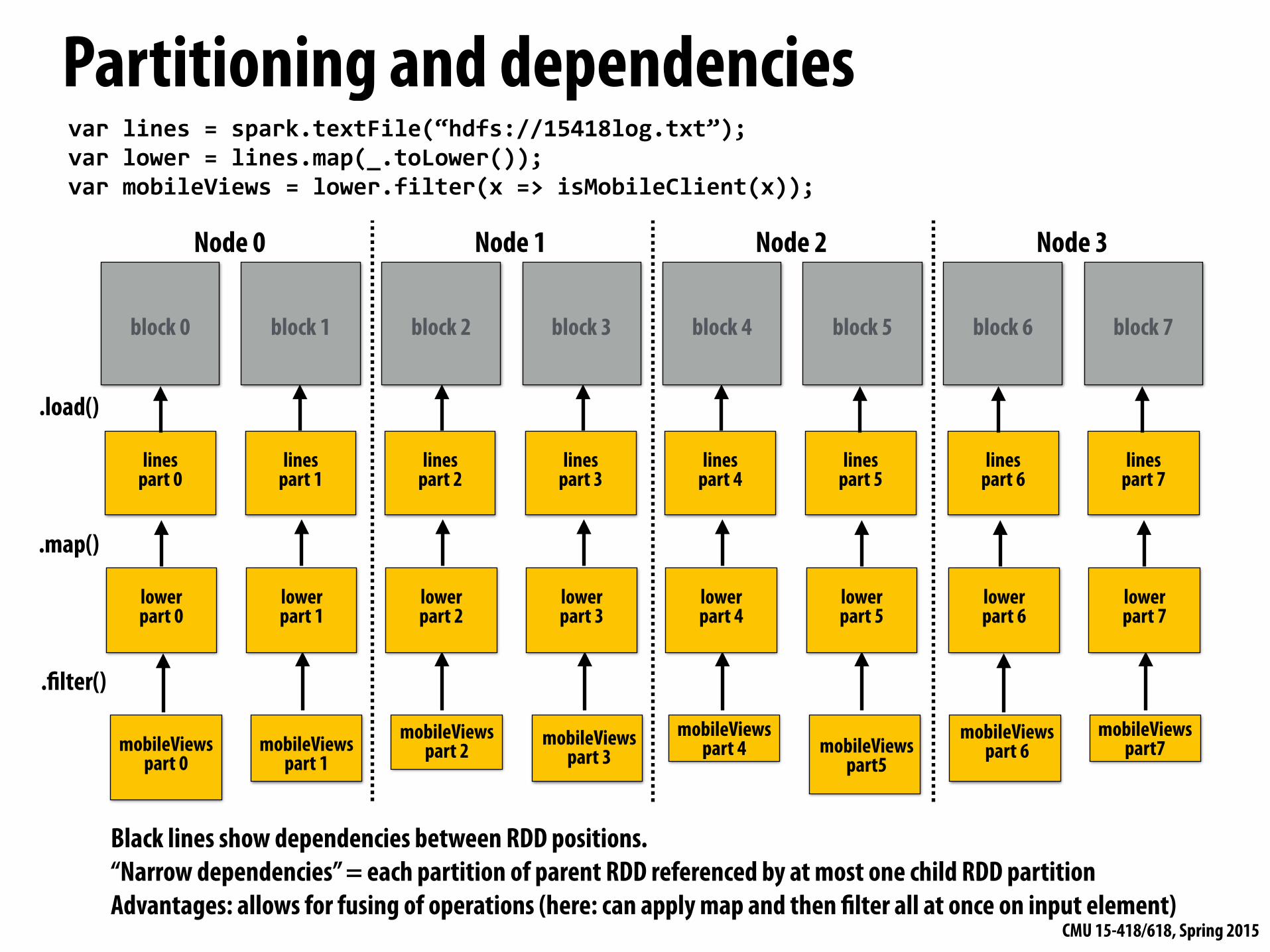
var lines = spark.textFile(“hdfs://15418log.txt”); var lower = lines.map(_.toLower()); var mobileViews = lower.filter(x => isMobileClient(x));
lines part 1
lines part 2
lines part 3
lines part 4
lines part 5
lines part 6
lines part 7
.filter()
mobileViews part 0
mobileViews part 1
mobileViews part 2 mobileViews
part 3mobileViews
part 4 mobileViews part5
mobileViews part 6
mobileViews part7
Black lines show dependencies between RDD positions. “Narrow dependencies” = each partition of parent RDD referenced by at most one child RDD partition Advantages: allows for fusing of operations (here: can apply map and then filter all at once on input element)
lower part 0
lower part 1
lower part 2
lower part 3
lower part 4
lower part 5
lower part 6
lower part 7
.map()

CMU 15-418/618, Spring 2015
Partitioning and dependencies
RDD_A part 0
.groupByKey()
RDD_A part 1
RDD_A part 2
RDD_A part 3
RDD_B part 0
RDD_B part 1
RDD_B part 2
RDD_B part 3
groupByKey: RDD[(K,V)], RDD[(K,W)] → RDD[(K,Seq[V])]
▪ Wide dependencies = each partition of parent RDD referenced by multiple child RDD partitions
▪ Challenges: - Must compute all of RDD_A before computing RDD_B (example: groupByKey
may induce all-to-all communication) - May trigger significant recompilation of ancestor lineage upon node failure

CMU 15-418/618, Spring 2015
Partitioning and dependenciesjoin: RDD[(K,V)], RDD[(K,W)] → RDD[(K,(V,W))]
RDD_C part 0
RDD_C part 1
RDD_C part 6
RDD_C part 9
.join()
RDD_A part 0
RDD_A part 1
RDD_A part 2
RDD_A part 3
RDD_B part 0
RDD_B part 1
RDD_B part 2
RDD_B part 3
(“Kayvon”, 1) (“Bob”, 23)
(“Kayvon”, “fizz”) (“Bob”, “buzz”)
(“Jane”, 1024) (“Li”, 32)
(“Jane”, “wham”) (“Li”, “pow”)
(“Will”, 50) (“Arjun”, 9)
(“Will”, “splat”) (“Arjun”, “pop”)
(“Cary”, 10) (“Vivek”, 100)
(“Cary”, “slap”) (“Vivek”, “bam”)
RDD_C part 0
RDD_C part 1
RDD_C part 6
RDD_C part 9
.join()
RDD_A part 0
RDD_A part 1
RDD_A part 2
RDD_A part 3
RDD_B part 0
RDD_B part 1
RDD_B part 2
RDD_B part 3
(“Kayvon”, 1) (“Bob”, 23)
(“Kayvon”, “fizz”) (“Will”, “splat”)
(“Jane”, 1024) (“Li”, 32)
(“Arjun”, “pop”) (“Cary”, “slap”)
(“Will”, 50) (“Arjun”, 9)
(“Li”, “pow”) (“Vivek”, “bam”)
(“Cary”, 10) (“Vivek”, 100)
(“Jane”, “wham”) (“Bob”, “buzz”)
(“Kayvon”, (1,”fizz”)) (“Bob”, (23,”buzz”))
(“Jane”, (1024,”wham”)) (“Li”, (32,”pow”))
(“Will”, (50,”splat”)) (“Arjun”, (9,”pop”))
(“Cary”, (10,”slap”)) (“Vivek”, (100,”bam”))
RDD_A and RDD_B have different hash partitions: join creates wide dependencies
RDD_A and RDD_B have same hash partition: join only create narrow dependencies
(“Kayvon”, (1,”fizz”)) (“Bob”, (23,”buzz”))
(“Jane”, (1024,”wham”)) (“Li”, (32,”pow”))
(“Will”, (50,”splat”)) (“Arjun”, (9,”pop”))
(“Cary”, (10,”slap”)) (“Vivek”, (100,”bam”))
CMU 15-418/618, Spring 2015
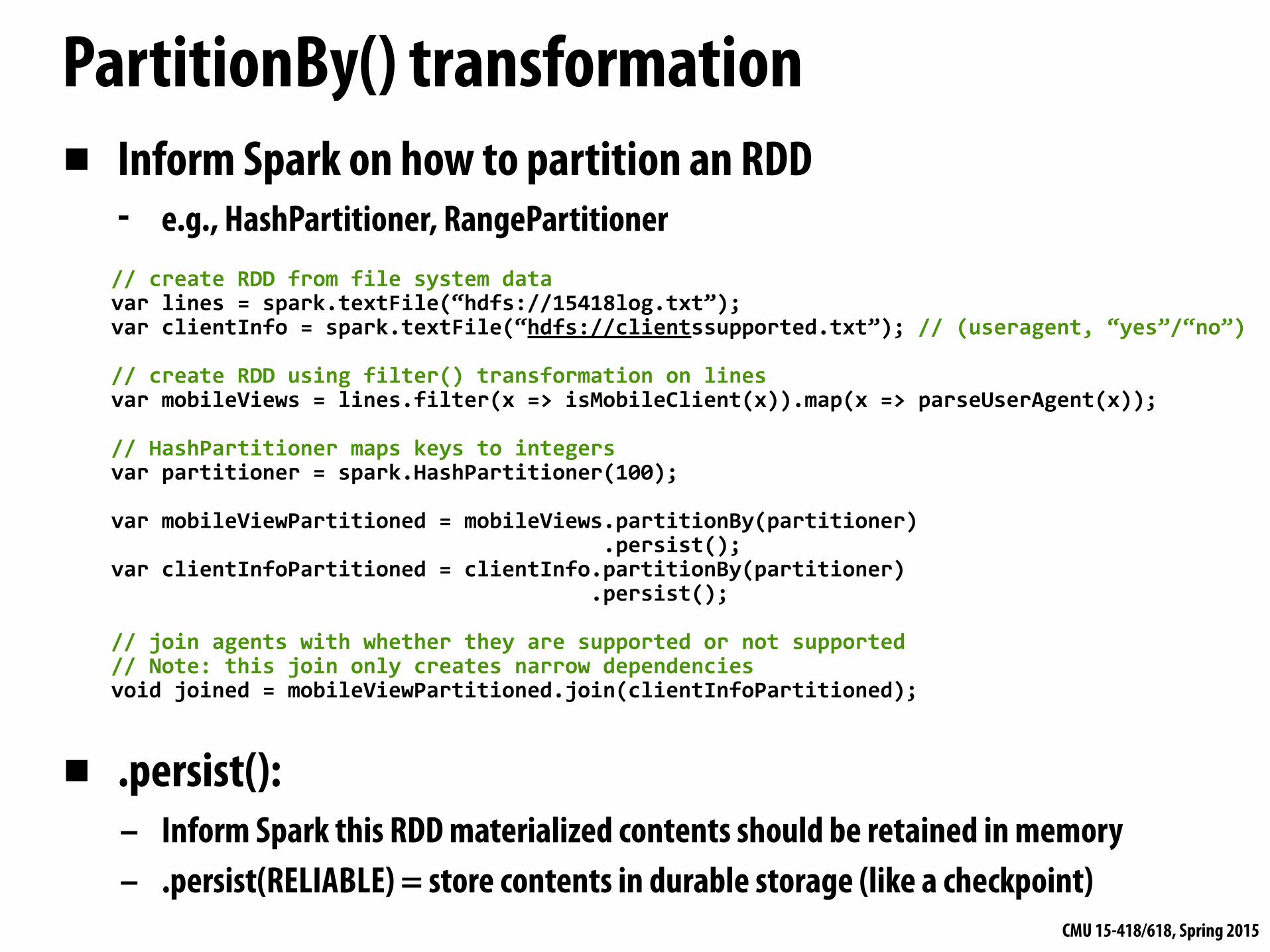
PartitionBy() transformation▪ Inform Spark on how to partition an RDD
- e.g., HashPartitioner, RangePartitioner// create RDD from file system data var lines = spark.textFile(“hdfs://15418log.txt”); var clientInfo = spark.textFile(“hdfs://clientssupported.txt”); // (useragent, “yes”/“no”)
// create RDD using filter() transformation on lines var mobileViews = lines.filter(x => isMobileClient(x)).map(x => parseUserAgent(x));
// HashPartitioner maps keys to integers var partitioner = spark.HashPartitioner(100);
var mobileViewPartitioned = mobileViews.partitionBy(partitioner) .persist(); var clientInfoPartitioned = clientInfo.partitionBy(partitioner) .persist();
// join agents with whether they are supported or not supported // Note: this join only creates narrow dependencies void joined = mobileViewPartitioned.join(clientInfoPartitioned);
▪ .persist(): - Inform Spark this RDD materialized contents should be retained in memory - .persist(RELIABLE) = store contents in durable storage (like a checkpoint)

CMU 15-418/618, Spring 2015
Scheduling Spark computations
Actions (e.g., save()) trigger evaluation of Spark lineage graph.
RDD_A part 0
RDD_A part 1
RDD_A part 2
RDD_B part 0
RDD_B part 1
RDD_B part 2
.groupByKey()
RDD_C part 0
RDD_C part 1
RDD_D part 0
RDD_D part 1
RDD_E part 0
RDD_E part 1
RDD_F part 0
RDD_F part 1
RDD_F part 2
RDD_F part 3
.map()
.union()
.join()
RDD_G part 0
RDD_G part 1
RDD_G part 2
.save()
Stage 1 Computation Stage 2 Computation
Stage 1 Computation: do nothing since input already materialized in memoryStage 2 Computation: evaluate map, only actually materialize RDD FStage 3 Computation: execute join (could stream the operation to disk, do not need to materialize )
block 1block 0 block 2 = materialized RDD
CMU 15-418/618, Spring 2015
Performancethem simpler to checkpoint than general shared mem-ory. Because consistency is not a concern, RDDs can bewritten out in the background without requiring programpauses or distributed snapshot schemes.
6 EvaluationWe evaluated Spark and RDDs through a series of exper-iments on Amazon EC2, as well as benchmarks of userapplications. Overall, our results show the following:• Spark outperforms Hadoop by up to 20⇥ in itera-
tive machine learning and graph applications. Thespeedup comes from avoiding I/O and deserializationcosts by storing data in memory as Java objects.
• Applications written by our users perform and scalewell. In particular, we used Spark to speed up an an-alytics report that was running on Hadoop by 40⇥.
• When nodes fail, Spark can recover quickly by re-building only the lost RDD partitions.
• Spark can be used to query a 1 TB dataset interac-tively with latencies of 5–7 seconds.
We start by presenting benchmarks for iterative ma-chine learning applications (§6.1) and PageRank (§6.2)against Hadoop. We then evaluate fault recovery in Spark(§6.3) and behavior when a dataset does not fit in mem-ory (§6.4). Finally, we discuss results for user applica-tions (§6.5) and interactive data mining (§6.6).
Unless otherwise noted, our tests used m1.xlarge EC2nodes with 4 cores and 15 GB of RAM. We used HDFSfor storage, with 256 MB blocks. Before each test, wecleared OS buffer caches to measure IO costs accurately.
6.1 Iterative Machine Learning ApplicationsWe implemented two iterative machine learning appli-cations, logistic regression and k-means, to compare theperformance of the following systems:• Hadoop: The Hadoop 0.20.2 stable release.
• HadoopBinMem: A Hadoop deployment that con-verts the input data into a low-overhead binary formatin the first iteration to eliminate text parsing in laterones, and stores it in an in-memory HDFS instance.
• Spark: Our implementation of RDDs.We ran both algorithms for 10 iterations on 100 GB
datasets using 25–100 machines. The key difference be-tween the two applications is the amount of computationthey perform per byte of data. The iteration time of k-means is dominated by computation, while logistic re-gression is less compute-intensive and thus more sensi-tive to time spent in deserialization and I/O.
Since typical learning algorithms need tens of itera-tions to converge, we report times for the first iterationand subsequent iterations separately. We find that shar-ing data via RDDs greatly speeds up future iterations.
80!
139!
46!
115!
182!
82!
76!
62!
3!
106!
87!
33!
0!40!80!
120!160!200!240!
Hadoop! HadoopBM! Spark! Hadoop! HadoopBM! Spark!
Logistic Regression! K-Means!
Itera
tion
time
(s)!
First Iteration!Later Iterations!
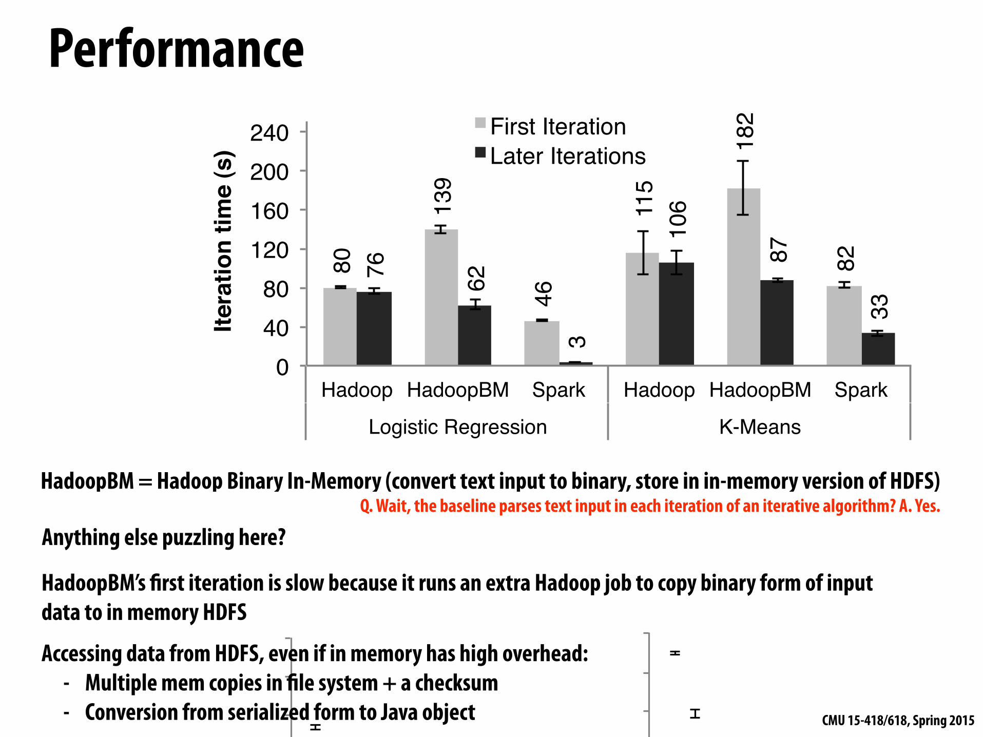
Figure 7: Duration of the first and later iterations in Hadoop,HadoopBinMem and Spark for logistic regression and k-meansusing 100 GB of data on a 100-node cluster.
184!
111!
76!
116!
80!
62!
15!
6! 3!
0!50!100!150!200!250!300!
25! 50! 100!
Itera
tion
time
(s)!
Number of machines!
Hadoop!HadoopBinMem!Spark!
(a) Logistic Regression
274!
157!
106!
197!
121!
87!
143!
61!
33!
0!
50!
100!
150!
200!
250!
300!
25! 50! 100!
Itera
tion
time
(s)!
Number of machines!
Hadoop !HadoopBinMem!Spark!
(b) K-Means
Figure 8: Running times for iterations after the first in Hadoop,HadoopBinMem, and Spark. The jobs all processed 100 GB.
First Iterations All three systems read text input fromHDFS in their first iterations. As shown in the light barsin Figure 7, Spark was moderately faster than Hadoopacross experiments. This difference was due to signal-ing overheads in Hadoop’s heartbeat protocol betweenits master and workers. HadoopBinMem was the slowestbecause it ran an extra MapReduce job to convert the datato binary, it and had to write this data across the networkto a replicated in-memory HDFS instance.
Subsequent Iterations Figure 7 also shows the aver-age running times for subsequent iterations, while Fig-ure 8 shows how these scaled with cluster size. For lo-gistic regression, Spark 25.3⇥ and 20.7⇥ faster thanHadoop and HadoopBinMem respectively on 100 ma-chines. For the more compute-intensive k-means appli-cation, Spark still achieved speedup of 1.9⇥ to 3.2⇥.
Understanding the Speedup We were surprised tofind that Spark outperformed even Hadoop with in-memory storage of binary data (HadoopBinMem) by a20⇥ margin. In HadoopBinMem, we had used Hadoop’sstandard binary format (SequenceFile) and a large blocksize of 256 MB, and we had forced HDFS’s data di-rectory to be on an in-memory file system. However,Hadoop still ran slower due to several factors:1. Minimum overhead of the Hadoop software stack,
2. Overhead of HDFS while serving data, and
HadoopBM = Hadoop Binary In-Memory (convert text input to binary, store in in-memory version of HDFS)
Anything else puzzling here?Q. Wait, the baseline parses text input in each iteration of an iterative algorithm? A. Yes.
HadoopBM’s first iteration is slow because it runs an extra Hadoop job to copy binary form of input data to in memory HDFS
Accessing data from HDFS, even if in memory has high overhead: - Multiple mem copies in file system + a checksum - Conversion from serialized form to Java object

CMU 15-418/618, Spring 2015
Spark summary▪ Introduces opaque collection abstraction (RDD) to encapsulate intermediates of
cluster computations (previously… frameworks stored intermediates in the file system) - Observation: “files are a poor abstraction for intermediate variables in large
scale data-parallel programs” - RDDs are read-only, and created by deterministic data-parallel operators - Lineage tracked and used for locality-aware scheduling and fault-tolerance
(allows recomputation of partitions of RDD on failure, rather than restore from checkpoint *) - Bulk operations allow overhead of lineage tracking (logging) to be low.
▪ Simple, versatile abstraction upon which many domain-specific distributed computing frameworks are being implemented. - See Apache Spark project: spark.apache.org
* Note that .persist(RELIABLE) allows programmer to request checkpointing in long lineage situations.

CMU 15-418/618, Spring 2015
Modern Spark ecosystem
Interleave computation and database query Can apply transformations to RDDs produced by SQL queries
Machine learning library build on top of Spark abstractions.
GraphLab-like library built on top of Spark abstractions.
Compelling feature: enables integration/composition of multiple domain-specific frameworks (since all collections implemented under the hood with RDDs and scheduled using Spark scheduler)
CMU 15-418/618, Spring 2015
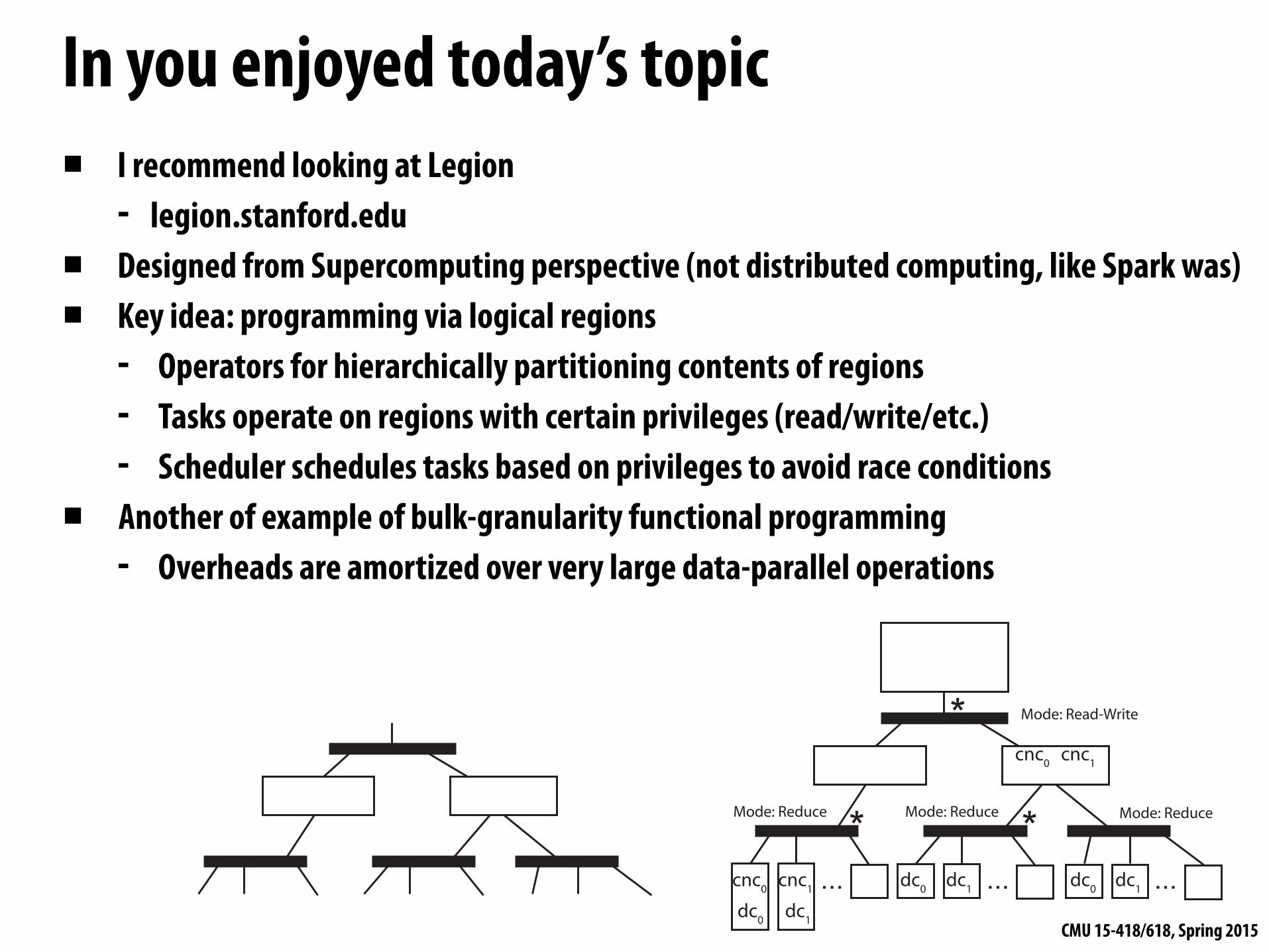
In you enjoyed today’s topic▪ I recommend looking at Legion
- legion.stanford.edu ▪ Designed from Supercomputing perspective (not distributed computing, like Spark was) ▪ Key idea: programming via logical regions
- Operators for hierarchically partitioning contents of regions - Tasks operate on regions with certain privileges (read/write/etc.) - Scheduler schedules tasks based on privileges to avoid race conditions
▪ Another of example of bulk-granularity functional programming - Overheads are amortized over very large data-parallel operations
... ... ...
*
* *cnc0 cnc0 cnc0cnc1 cnc1 cnc1
Mode: Read-Write Mode: Read-Only Mode: Read-Only
Mode: Read-Write
(a) Two calc_new_currents
tasks.
... ... ...
*
* *
dc0
dc0 dc0
dc1
dc1 dc1
Mode: Reduce Mode: Reduce Mode: Reduce
Mode: Read-Write
cnc0 cnc1
cnc0 cnc1
(b) distribute_charge dependson calc_new_currents.
... ... ...
*
* *
uv0
uv0
uv1
uv1
Mode: Read-Write Mode: Read-Write Mode: None
Mode: Read-Write
dc0 dc1
cnc0 cnc1
cnc0 cnc1dc0 dc1
(c) update_voltages depends ondistribute_charge.
... ... ...
*
* *dc0
All-Shared
reductions
copy
dc0dc1 dc1dcn-1 dcn-1
uv0
(d) An update_voltages map-ping.
Fig. 3. Dependence analysis examples from circuit_simulation.
a writer does not require a valid instance—becausereductions can be reordered, combining the instancesof r and r0 (if they alias) can be deferred to a laterconsumer of the data (see case 4).
4) If t0 has reduce privilege for r0 and t has read, write,or reduce privileges with a different operator than t0 forr, and r aliases r0, then s0 must be reduced (using t0’sreduction operator) to an instance s00 of r t r0 and thena fresh instance of r created from s00. Instance s0 isremoved from the region tree.
To map r, we walk from r’s root ancestor in the region forestto r, along the way exploring off-path subtrees to find regioninstances satisfying cases 2 and 4. The details and analysisare similar to the implementation of dependence analysisin Section III-A; the amortized work per region mapped isproportional to the depth of the region forest and independentof the number of tasks or physical instances.
As part of the walk any required copy and reductionoperations are issued to construct a valid instance of r. Theseoperations are deferred, waiting to execute on the tasks thatproduce the data they copy or reduce. Similarly, the startof t’s execution is made dependent on completion of thecopies/reductions that construct the instance of r it will use.
Figure 3(d) shows part of the mapping of taskupdate_voltages[0]; we focus only on theshared nodes. Because the immediately precedingdistribute_charges tasks all performed the samereduction on the shared and ghost nodes they were allowedto run in parallel. But update_voltages[0] needsread/write privilege for pieces[0].rn_shr, which forcesall of the reductions to be merged back to an instanceof the all-shared nodes region, from which a newinstance of pieces[0].rn_shr is copied and used byupdate_voltages[0].
D. Stage 4: Execution
After a task t has been mapped it enters the execution stageof the SOOP. When all of the operations (other tasks andcopies) on which t depends have completed, t is launchedon the processor it was mapped to. When t spawns subtasks,they are registered by the SOOP on which t is executing, usingt as the parent task and t’s region arguments as the roots ofthe region forest. Each child of t traverses the SOOP pipelineon the same processor as t, possibly being mapped to a SOOPinstance on a different processor to execute.
E. Stage 5: Clean-Up
Once task t is done executing its state is reclaimed.Dependence and mapping information is removed from theregion tree. The most involved aspect of clean-up is collectingphysical instances that are no longer in use, for which we usea distributed reference counting scheme.
IV. MAPPING INTERFACE
As mentioned previously, a novel aspect of Legion is themapping interface, which gives programmers control overwhere tasks run and where region instances are placed, makingpossible application- or machine-specific mapping decisionsthat would be difficult for a general-purpose programmingsystem to infer. Furthermore, this interface is invoked atruntime which allows for dynamic mapping decisions based onprogram input data. We describe the interface (Section IV-A),our base implementation (Section IV-B), and the benefits ofcreating custom mappers (Section IV-C).
A. The Interface
The mapping interface consists of ten methods that SOOPscall for mapping decisions. A mapper implementing thesemethods has access to a simple interface for inspecting proper-ties of the machine, including a list of processors and their type(e.g. CPU, GPU), a list of memories visible to each processor,and their latencies and bandwidths. For brevity we only discussthe three most important interface calls:
• select_initial_processor - For each task t inits mapping queue a SOOP will ask for a processor fort. The mapper can keep the task on the local processoror send it to any other processor in the system.
• permit_task_steal - When handling a steal requesta SOOP asks which tasks may be stolen. Stealing can bedisabled by always returning the empty set.
• map_task_region - For each logical region r usedby a task, a SOOP asks for a prioritized list of mem-ories where a physical instance of r should be placed.The SOOP provides a list of r’s current valid physicalinstances; the mapper returns a priority list of memoriesin which the SOOP should attempt to either reuse orcreate a physical instance of r. Beginning with the firstmemory, the SOOP uses a current valid instance if oneis present. Otherwise, the SOOP attempts to allocate aphysical instance and issue copies to retrieve the validdata. If that also fails, the SOOP moves on to the nextmemory in the list.


