
23-1
Lecture 23
Multiple Comparisons & Contrasts
STAT 512
Spring 2011
Background Reading
KNNL: 17.3-17.7

23-2
Topic Overview
• Linear Combinations and Contrasts
• Pairwise Comparisons and Multiple Testing
Adjustments
23-3
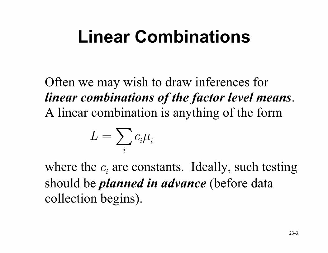
Linear Combinations
Often we may wish to draw inferences for
linear combinations of the factor level means.
A linear combination is anything of the form
i i
i
L c µ=∑
where the ic are constants. Ideally, such testing
should be planned in advance (before data
collection begins).

23-4
Cash Offers Example #1
• Suppose that 30% of those trading a car are
young, 60% middle aged, and 10% elderly.
We would like to estimate the mean offer,
taking into account these weights.
• We use a linear combination
0.3 0.6 0.1yng mid eldL µ µ µ= + +

23-5
Estimate for L
• In general, if i i
i
L c µ=∑ , an unbiased
estimate for L will be ˆ i i
i
L cY=∑ i
• Variance for estimate can be derived from
independence of the factor level means:
( ) ( )2
2 2ˆ i
i ii i i
cVar L cVar Y
nσ= =∑ ∑i
• Standard error is: � ( )2
ˆ i
i i
cSE L MSE
n= ∑

23-6
Hypothesis Tests & CI’s
• Test 0 0:H L L= against 0 0:H L L≠
• Test statistic is given by
� ( )
* 0ˆ
ˆ
L Lt
SE L
−=
• Compare to T-critical value using degrees of
freedom for error from the model.
• Confidence interval can be developed by using
� ( )ˆ ˆcritL t SE L±

23-7
CO Example #1 (2)
• For the cash offers data, 12 observations per group. So the standard error for
0.3 0.6 0.1yng mid eldL µ µ µ= + +
will be:
� ( ) ( )2 2 20.3 0.6 0.1
12 12 12ˆ
2.49 0.03833 0.3089
SE L MSE= + +
= × =

23-8
CO Example #1 (3)
• We could construct a confidence interval for L:
� ( )ˆ ˆcritL t SE L±
( ) ( ) ( )ˆ 0.3 21.5 0.6 27.75 0.1 21.4167L = + + =25.24
Here 0.975(33) 2.03452
critt t= =
• So, the 95% confidence interval for L is:
25.24±2.03452*0.3089 = (24.61, 25.87)

23-9
Contrasts
• A contrast is any linear combination for
which the sum of the coefficients is zero
(that is, for which 0ic =∑ )
• EVERY PAIRWISE COMPARISON IS A CONTRAST!!!!! ( 'i iL µ µ= − )
• Contrasts additionally used to compare
groups of means.

23-10
Cash Offers Example #2
• Suppose our initial belief is that middle aged
people will be more successful in trading
their cars than will young or elderly.
• Then an appropriate contrast is: 0.5 0.5mid eld yngL µ µ µ= − −
• We could do a one-sided test here based on
our initial hypothesis.
0: 0 vs. : 0
aH L H L≤ >
• Advantage: No multiple comparison issues
here if this test is our goal from the start.
23-11
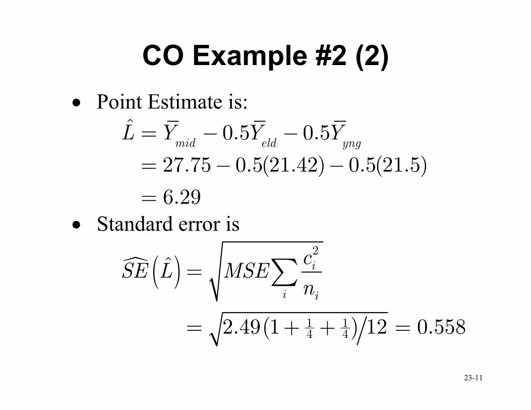
CO Example #2 (2)
• Point Estimate is:
ˆ 0.5 0.5
27.75 0.5(21.42) 0.5(21.5)
6.29
mid eld yngL Y Y Y= − −
= − −
=
• Standard error is
� ( )
( )
2
1 14 4
ˆ
2.49 1 12 0.558
i
i i
cSE L MSE
n=
= + + =
∑

23-12
CO Example #2 (3)
• Test statistic:
� ( )* 0ˆ 6.29
11.28ˆ 0.558
L Lt
SE L
−= = =
• Compare to: 1 0.95
(33)tα− =
=1.69 – (One sided)
• Since t*>1.69, we reject the null hypothesis and conclude that there is a difference
between sales for middle aged when
compared to the average of the other two
groups

23-13
CO Example – SAS (cashoffers.sas)
proc glm data =cash; class age; model offer=age; contrast 'Comp #1' age - 0.5 1 - 0.5; estimate 'Est #1' age - 0.5 1 - 0.5; Contrast DF Contrast SS MS F Value Pr > F
Comp #1 1 316.68 316.68 127.2 <.0001
Param Estimate StdError t Value Pr>|t|
Est #1 6.29 0.558 11.28 <.0001
Note: 11.28*11.28 = 127.2

23-14
ANOVA F-test: Relationship to Contrasts
• Null hypothesis is that all means are equal
• Alternative hypothesis is that some means
are not equal. Often we write this as “there
exists some i jµ µ≠ .
• This alternative isn’t 100% accurate. In fact
we are actually considering simultaneously
ALL POSSIBLE CONTRASTS.

23-15
F-test (2)
• So rejection in the ANOVA F-test really means “there exists some non-zero contrast
of the means”.
• This means it is entirely possible to find a
significant overall F-test, but have no
significant pairwise comparisons (the p-
value for the F-test will generally be fairly
close to 0.05 if this occurs).

23-16
F-test (3)
• We are even less likely to find pairwise differences
when we adjust the critical values for multiple
comparisons.
• One possible algorithmic procedure to find
differences would be to look at the F-test, then if
it is significant, look at unadjusted pairwise
comparisons. This is just the LSD multiple
comparison procedure.

23-17
Multiple Comparison Procedures
• Least Significant Differences (LSD)
o No adjustment
• Tukey (or Tukey-Kramer)
• Bonferroni
• Scheffe

23-18
Least Significant Differences
• Least significant difference is given by
1 /2
1 1( )T
i i
LSD t n r MSEn nα−
′
= − +
• If the F-test indicates that a factor is significant, then any pair of means that
differ by at least LSD are considered to be
different.

23-19
LSD (2)
• This is the least conservative of all the procedures, because no adjustment is made
for multiple comparisons (so when doing
lots of comparisons this makes Type I
errors likely)
• Generally prefer to have strongly significant F-test (say p-value < 0.01 or 0.005) before
looking at LSD comparisons.

23-20
LSD (3)
• Procedure is really too liberal, but the good part of this tradeoff is that it will also have
greater power than any of the other tests
we will discuss.
• Called either ‘t’ or ‘lsd’ in the MEANS
statement of PROC GLM

23-21
Cash Offers Example
proc glm data =cash; class age; model offer=age; means age / lines t ;
• F = 63.6, p-value < 0.0001
• Since significant, look at LSD = 1.31
Mean N age
A 27.7500 12 Middle
B 21.5000 12 Young
B 21.4167 12 Elderly

23-22
Tukey Procedure
• Specifies an EXACT family significance
level for comparing ALL PAIRS OF
TREATMENT MEANS.
• Is more conservative (and generally more
appropriate than LSD)
• Controls the alpha level, tradeoff is having less power

23-23
Tukey Procedure (2)
• Based on the studentized range distribution (critical values cq found in table B9)
• Actual critical value is / 2cq ; numerator
and denominator degrees of freedom are r
and nT – r, respectively.
• Minimum significant difference is given by
1 ( , ) 1 1
2
Tr n r
i i
qMSE
n n
α− −
′
+

23-24
Tukey Procedure (3)
• Use to develop hypothesis tests and confidence intervals
• For any difference in means D, testing
0 : 0 vs. : 0aH D H D= ≠
• 95% CI is given by
( ) 1( , ) 1 1
2
T
i i
i i
q r n rY Y MSE
n nα−
′
′
− − ± + i i
Use ‘tukey’ in MEANS statement in PROC GLM

23-25
Cash Offers Example
proc glm data =cash; class age; model offer=age; means age / lines tukey ;
Critical Value of Studentized Range 3.47019
Minimum Significant Difference 1.5807
Mean N age
A 27.7500 12 Middle
B 21.5000 12 Young
B 21.4167 12 Elderly

23-26
Bonferroni Procedure
• We know the idea (divide alpha by the
number of tests/CI’s).
• Sacrifices slightly more power than
TUKEY, but can be applied to any set of
contrasts or linear combinations (useful in
more situations than Tukey).
• Is usually better than Tukey if we want to do a small number of planned comparisons.

23-27
Bonferroni Procedure (2)
• For all g = ( )12 1r r − pairwise comparisons,
minimum significant difference is
1 /2
1 1( )g T
i i
t n r MSEn nα−
′
− +
• CI’s given by
( ) 1 /2
1 1( )
i i g T
i i
Y Y t n r MSEn nα′ −
′
− ± − +
i i

23-28
Cash Offers Example
proc glm data =cash; class age; model offer=age; means age / lines bon ; Critical Value of t 2.52221
Minimum Significant Difference 1.6248
Mean N age
A 27.7500 12 Middle
B 21.5000 12 Young
B 21.4167 12 Elderly

23-29
Scheffe Comparison Procedure
• Most conservative (least powerful) of all
tests. Protects against data snooping!
• Controls the family alpha level for testing
ALL POSSIBLE CONTRASTS
• Should be used if you have not planned contrasts in advance.
23-30
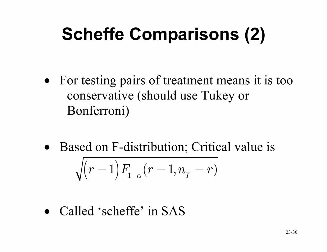
Scheffe Comparisons (2)
• For testing pairs of treatment means it is too
conservative (should use Tukey or
Bonferroni)
• Based on F-distribution; Critical value is
( ) 11 ( 1, )
Tr F r n r
α−− − −
• Called ‘scheffe’ in SAS

23-31
Cash Offers Example
proc glm data =cash; class age; model offer=age; means age / lines scheffe ;
Critical Value of F 3.28492
Minimum Significant Difference 1.6512
Mean N age
A 27.7500 12 Middle
B 21.5000 12 Young
B 21.4167 12 Elderly

23-32
Cash Offers Example
Comparison
Type
Critical
Value
Minimum
Significant
Difference
LSD t = 2.03 1.31
Tukey / 2 2.45q = 1.58
Bonferroni t = 2.52 1.62
Scheffe f = 3.28 1.65
Cell Sizes: Equal, n = 12, r = 3

23-33
Procedure Usage Summary
• Use BONFERRONI when only interested in a small number of planned contrasts (or
pairwise comparisons)
• Use TUKEY when only interested in all (or most) pairwise comparisons of means
• Use SCHEFFE when doing anything that could be considered data snooping – i.e.
for any unplanned contrasts

23-34
Significance Level vs. Power
Most
Powerful LSD
Least
Conservative
Tukey
Bonferroni
Least
Powerful Scheffe
Most
Conservative

23-35
Further Comments
• Bonferroni may be better than Tukey (or
Scheffe) when the number of contrasts of
interest is about the same as the number of
groups (r). Remember to use this the
contrasts should be pre-planned.
• All procedures yield confidence limits of the
form
EST CRIT SE± ×

23-36
Other Comparison Procedures
• DUNCAN = Duncan’s Multiple Range Test
(used for pairwise comparisons; similar to
TUKEY)
• DUNNETT(‘control’) = DUNNETT’s test for comparing treatments vs. control (r – 1)
tests; better than Bonferroni for this often-
encountered specific situation

23-37
Example (Kenton Food Co.)
• Recall testing 4 box designs, 5 stores each.
• Response: Number of cases sold
• One design has only 4 observations since one store burned during the study
• F = 18.56; p-value < 0.0001 implies we
should look for some difference among the
means
• SAS code: kenton.sas

23-38
Kenton Example #1 (1)
• Suppose goal is “rank” the box designs and determine if any significant differences in
their mean number of cases sold.
• To accomplish this, look at all pairwise
comparisons.
• We will examine results using:
o Least significant difference – too liberal
o Tukey – Preferred method
o Bonferroni – Possibly reasonable here
o Scheffe –too conservative

23-39
Kenton Example #1 (2)
*Pairwise Comparisons using different multiple adjustment methods; proc glm data =kenton; class design; model cases=design; means design / lines t tukey bon scheffe ; means design / cldiff t tukey bon scheffe ; run;

23-40
Kenton Example #1 (3) LSD Results
Error Mean Square 10.54667
Critical Value of t 2.13145
Least Significant Difference 4.5126
Harmonic Mean of Cell Sizes 4.705882
NOTE: Cell sizes are not equal.
• SAS uses slightly different method to
determine a single “least significant
difference” even when the cell sizes are
unequal (some kind of weighted average)

23-41
Kenton Example #1 (4)
LSD Results
A 27.200 5 4
B 19.500 4 3
C 14.600 5 1
C
C 13.400 5 2
23-42
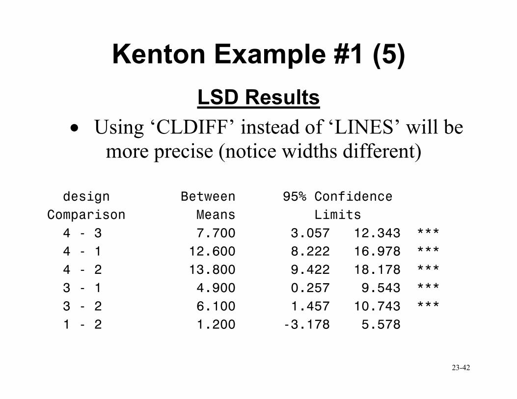
Kenton Example #1 (5)
LSD Results
• Using ‘CLDIFF’ instead of ‘LINES’ will be more precise (notice widths different)
design Between 95% Confidence
Comparison Means Limits
4 - 3 7.700 3.057 12.343 ***
4 - 1 12.600 8.222 16.978 ***
4 - 2 13.800 9.422 18.178 ***
3 - 1 4.900 0.257 9.543 ***
3 - 2 6.100 1.457 10.743 ***
1 - 2 1.200 -3.178 5.578

23-43
Kenton Example #1 (6) Tukey Results
Critical Value of Studentized Range 4.07597
Minimum Significant Difference 6.1019
Harmonic Mean of Cell Sizes 4.705882
NOTE: Cell sizes are not equal.
A 27.200 5 4
B 19.500 4 3
B
B 14.600 5 1
B
B 13.400 5 2

23-44
Kenton Example #1 (7) Tukey Results
design Between Simultaneous 95%
Comparison Means Confidence Limits
4 - 3 7.700 1.421 13.979 ***
4 - 1 12.600 6.680 18.520 ***
4 - 2 13.800 7.880 19.720 ***
3 - 1 4.900 -1.379 11.179
3 - 2 6.100 -0.179 12.379
1 - 2 1.200 -4.720 7.120
23-45
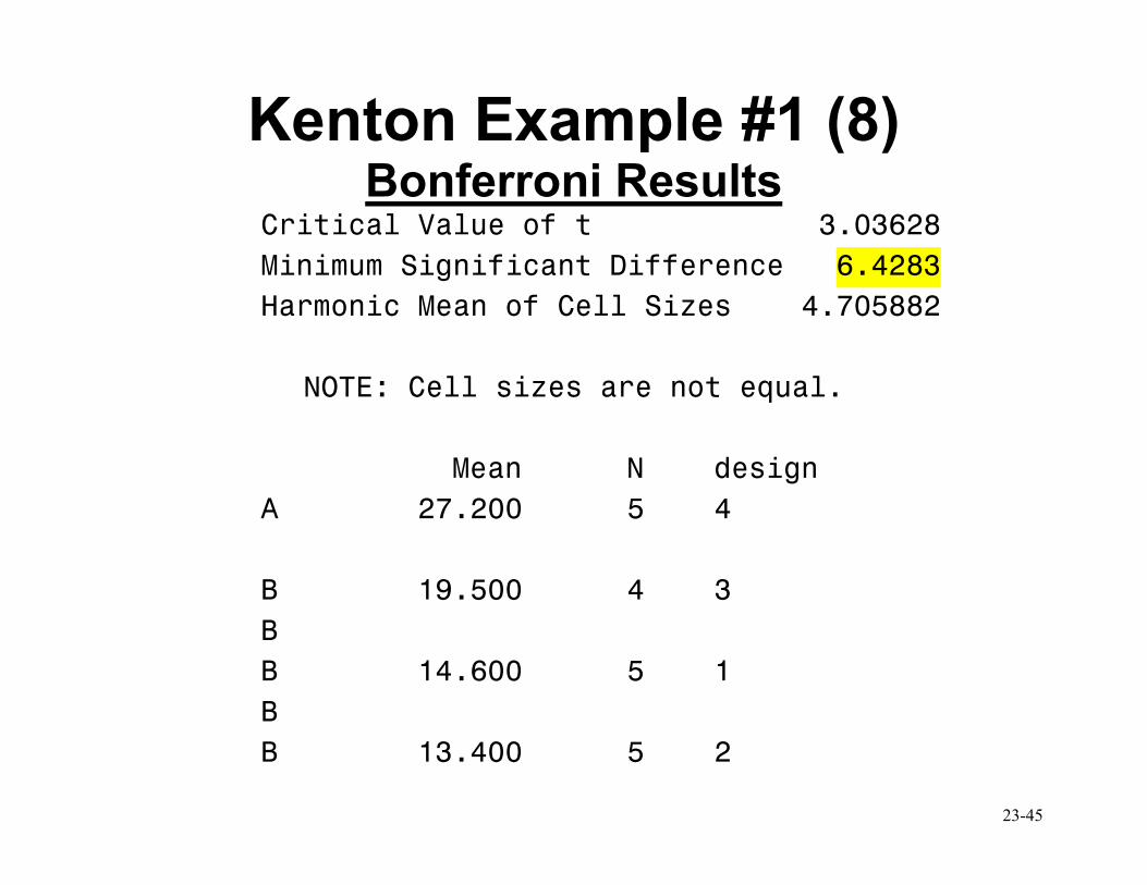
Kenton Example #1 (8) Bonferroni Results
Critical Value of t 3.03628
Minimum Significant Difference 6.4283
Harmonic Mean of Cell Sizes 4.705882
NOTE: Cell sizes are not equal.
Mean N design
A 27.200 5 4
B 19.500 4 3
B
B 14.600 5 1
B
B 13.400 5 2

23-46
Kenton Example #1 (9) Bonferroni Results
design Between Simultaneous 95%
Comparison Means Confidence Limits
4 - 3 7.700 1.085 14.315 ***
4 - 1 12.600 6.364 18.836 ***
4 - 2 13.800 7.564 20.036 ***
3 - 1 4.900 -1.715 11.515
3 - 2 6.100 -0.515 12.715
1 - 2 1.200 -5.036 7.436

23-47
Kenton Example #1 (10) Scheffe Results
Critical Value of F 3.28738
Minimum Significant Difference 6.6487
Harmonic Mean of Cell Sizes 4.705882
NOTE: Cell sizes are not equal.
Mean N design
A 27.200 5 4
B 19.500 4 3
B
B 14.600 5 1
B
B 13.400 5 2

23-48
Kenton Example #1 (11) Scheffe Results
design Between Simultaneous 95%
Comparison Means Confidence Limits
4 - 3 7.700 0.859 14.541 ***
4 - 1 12.600 6.150 19.050 ***
4 - 2 13.800 7.350 20.250 ***
3 - 1 4.900 -1.941 11.741
3 - 2 6.100 -0.741 12.941
1 - 2 1.200 -5.250 7.650

23-49
Kenton Example #1 (12) • We could order the boxes according to
their means: 2,1,3, 4 (least –greatest)
• If no multiple comparison adjustment is used (LSD), we find significant differences between all of the boxes except 1 and 2.
• Although Tukey is preferred, in this case, all three multiple comparison methods (Tukey, Bonferroni, Scheffe) lead to the same result: 4 is significantly different from the other boxes, but they are not significantly different from each other.

23-50
Kenton Example #2 (1) • After reviewing means, desire to show that
the mean for the 4th design is higher than
for the other designs
• Considering contrast:
4 1 2 33L µ µ µ µ= − − −
• Estimate statement yields Param Est StdError t Value Pr > |t|
Est 34.1 5.083 6.71 <.0001

23-51
Kenton Example #2 (2)
• Means statement with ‘Scheffe’ yields Critical Value of F 3.28738
• So ( ) ( )1 3 3.29 3.14r F− = =
• Since statistic = 6.71 is bigger than 3.14, we would reject the null and conclude that the
4th cereal is different from the other three
(combined)

23-52
Upcoming in Lecture 24...
• Review of Miscellaneous Issues in
Hypothesis Testing
• PROC POWER example
![COMP 333 Data Analytics [2ex] Exploratory Data Analysisusers.encs.concordia.ca/~gregb/home/PDF/comp333-eda.pdf · Exploratory Data Analysis Tukey 1977 book John Tukey (1977), Exploratory](https://cdn.vdocuments.us/doc/165x107/6014a0de4bad7c5bfa790925/comp-333-data-analytics-2ex-exploratory-data-gregbhomepdfcomp333-edapdf.jpg)


