Download - Lecture 15 Heat - ERNET

Lecture 15
Heat
6
EPS 122: Lecture 18 – Heat sources and flow
One layer model Equilibrium geotherms
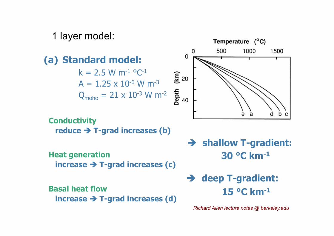
(a) Standard model: k = 2.5 W m-1 °C-1
A = 1.25 x 10⁻⁶ W m-3
Qmoho = 21 x 10-3 W m-2
� shallow T-gradient: 30 °C km-1
� deep T-gradient: 15 °C km-1
Conductivity reduce � T-grad increases (b)
Heat generation increase � T-grad increases (c)
Basal heat flow increase � T-grad increases (d)
EPS 122: Lecture 18 – Heat sources and flow
Two layer model Equilibrium geotherms
…more realistic
Consider each layer separately and match T and T-grad at boundary
A = A1
for 0 � z < z1
A = A2
for z1 � z < z2
layer 1
layer 2
and T = 0 at z = 0
Q = -Q2 at z = z2
for 0 � z < z1
for z1 � z < z2
6
EPS 122: Lecture 18 – Heat sources and flow
One layer model Equilibrium geotherms
(a) Standard model: k = 2.5 W m-1 °C-1
A = 1.25 x 10⁻⁶ W m-3
Qmoho = 21 x 10-3 W m-2
� shallow T-gradient: 30 °C km-1
� deep T-gradient: 15 °C km-1
Conductivity reduce � T-grad increases (b)
Heat generation increase � T-grad increases (c)
Basal heat flow increase � T-grad increases (d)
EPS 122: Lecture 18 – Heat sources and flow
Two layer model Equilibrium geotherms
…more realistic
Consider each layer separately and match T and T-grad at boundary
A = A1
for 0 � z < z1
A = A2
for z1 � z < z2
layer 1
layer 2
and T = 0 at z = 0
Q = -Q2 at z = z2
for 0 � z < z1
for z1 � z < z2
1 layer model:
6
EPS 122: Lecture 18 – Heat sources and flow
One layer model Equilibrium geotherms
(a) Standard model: k = 2.5 W m-1 °C-1
A = 1.25 x 10⁻⁶ W m-3
Qmoho = 21 x 10-3 W m-2
� shallow T-gradient: 30 °C km-1
� deep T-gradient: 15 °C km-1
Conductivity reduce � T-grad increases (b)
Heat generation increase � T-grad increases (c)
Basal heat flow increase � T-grad increases (d)
EPS 122: Lecture 18 – Heat sources and flow
Two layer model Equilibrium geotherms
…more realistic
Consider each layer separately and match T and T-grad at boundary
A = A1
for 0 � z < z1
A = A2
for z1 � z < z2
layer 1
layer 2
and T = 0 at z = 0
Q = -Q2 at z = z2
for 0 � z < z1
for z1 � z < z2
Richard Allen lecture notes @ berkeley.edu

6
EPS 122: Lecture 18 – Heat sources and flow
One layer model Equilibrium geotherms
(a) Standard model: k = 2.5 W m-1 °C-1
A = 1.25 x 10⁻⁶ W m-3
Qmoho = 21 x 10-3 W m-2
� shallow T-gradient: 30 °C km-1
� deep T-gradient: 15 °C km-1
Conductivity reduce � T-grad increases (b)
Heat generation increase � T-grad increases (c)
Basal heat flow increase � T-grad increases (d)
EPS 122: Lecture 18 – Heat sources and flow
Two layer model Equilibrium geotherms
…more realistic
Consider each layer separately and match T and T-grad at boundary
A = A1
for 0 � z < z1
A = A2
for z1 � z < z2
layer 1
layer 2
and T = 0 at z = 0
Q = -Q2 at z = z2
for 0 � z < z1
for z1 � z < z2
7
EPS 122: Lecture 18 – Heat sources and flow
U.S. temperatures
Estimated temperatures at 6 kilometers depth Data used: thermal conductivity, thickness of sedimentary rock, geothermal gradient, heat flow, and surface temperature.
Why the differences?
EPS 122: Lecture 18 – Heat sources and flow
Timescales …long
Increase basal heat from (a) Qmoho = 21 x 10-3 W m-2
to (d) Qmoho = 42 x 10-3 W m-2
Consider rock at 20 km depth
t = 0 567 °C
t = 20 Ma 580 °C
t = 100 Ma 700 °C
t = � 734 °C
� melting and intrusion are important heat transfer mechanisms in the lithosphere
Timescales
7
EPS 122: Lecture 18 – Heat sources and flow
U.S. temperatures
Estimated temperatures at 6 kilometers depth Data used: thermal conductivity, thickness of sedimentary rock, geothermal gradient, heat flow, and surface temperature.
Why the differences?
EPS 122: Lecture 18 – Heat sources and flow
Timescales …long
Increase basal heat from (a) Qmoho = 21 x 10-3 W m-2
to (d) Qmoho = 42 x 10-3 W m-2
Consider rock at 20 km depth
t = 0 567 °C
t = 20 Ma 580 °C
t = 100 Ma 700 °C
t = � 734 °C
� melting and intrusion are important heat transfer mechanisms in the lithosphere
8
EPS 122: Lecture 18 – Heat sources and flow
Timescales
From the diffusion equation we can define the
characteristic timescale
thermal diffusivity
the amount of time necessary for a temperature change to propagate a distance l
characteristic thermal diffusion distance
the distance a change in temperature will propagate in time �
thermal diffusivity of granite: 8.5 x 10⁻⁷ m2 s-1 l = 10 m � � = 4 years l = 1 km � � = 37,000 years l = 100 km � � = 370 Ma
EPS 122: Lecture 18 – Heat sources and flow
Instantaneous cooling
T0
T = 0 Semi-infinite half-space at temperature T0
Allow to cool at surface where T = 0
No internal heating, use diffusion equation
The solution is the error function
Characteristic timescale: Characteristic thermal diffusion distance:
8
EPS 122: Lecture 18 – Heat sources and flow
Timescales
From the diffusion equation we can define the
characteristic timescale
thermal diffusivity
the amount of time necessary for a temperature change to propagate a distance l
characteristic thermal diffusion distance
the distance a change in temperature will propagate in time �
thermal diffusivity of granite: 8.5 x 10⁻⁷ m2 s-1 l = 10 m � � = 4 years l = 1 km � � = 37,000 years l = 100 km � � = 370 Ma
EPS 122: Lecture 18 – Heat sources and flow
Instantaneous cooling
T0
T = 0 Semi-infinite half-space at temperature T0
Allow to cool at surface where T = 0
No internal heating, use diffusion equation
The solution is the error function
Melting and intrusion important heat transfer mechanisms in the lithosphere

8
EPS 122: Lecture 18 – Heat sources and flow
Timescales
From the diffusion equation we can define the
characteristic timescale
thermal diffusivity
the amount of time necessary for a temperature change to propagate a distance l
characteristic thermal diffusion distance
the distance a change in temperature will propagate in time �
thermal diffusivity of granite: 8.5 x 10⁻⁷ m2 s-1 l = 10 m � � = 4 years l = 1 km � � = 37,000 years l = 100 km � � = 370 Ma
EPS 122: Lecture 18 – Heat sources and flow
Instantaneous cooling
T0
T = 0 Semi-infinite half-space at temperature T0
Allow to cool at surface where T = 0
No internal heating, use diffusion equation
The solution is the error function
Richard Allen lecture [email protected]
8
EPS 122: Lecture 18 – Heat sources and flow
Timescales
From the diffusion equation we can define the
characteristic timescale
thermal diffusivity
the amount of time necessary for a temperature change to propagate a distance l
characteristic thermal diffusion distance
the distance a change in temperature will propagate in time �
thermal diffusivity of granite: 8.5 x 10⁻⁷ m2 s-1 l = 10 m � � = 4 years l = 1 km � � = 37,000 years l = 100 km � � = 370 Ma
EPS 122: Lecture 18 – Heat sources and flow
Instantaneous cooling
T0
T = 0 Semi-infinite half-space at temperature T0
Allow to cool at surface where T = 0
No internal heating, use diffusion equation
The solution is the error function
3
EPS 122: Lecture 19 – Geotherms
Instantaneous cooling
T = T0
T = 0 Semi-infinite half-space at temperature T0
Allow to cool at surface where T = 0
No internal heating, use diffusion equation
The solution is the error function
time t1 � calc error func � T = 0.9T0
time t2 � calc error func � T = 0.6T0
time
EPS 122: Lecture 19 – Geotherms
Oceanic heat flow – observations
Stei
n &
Ste
in, 1
994
•� Higher for younger crust (mostly)
•� Greater variability for younger crust
� hydrothermal circulation at mid-ocean ridges
Non-steady state case

Error function
Q(z) =�k
∂T
∂z
∂T
∂t
=k
rC
p
—2T +
A
rC
p
∂T
∂t
=k
rC
p
—2T +
A
rC
p
�u ·—T
∂2T
∂z
2 =�A
k
Q =�k
∂T
∂z
=�Q0
T =� A
2k
z
2 +(Q
d
+Ad)
k
z
er f (x) =2pp
Zx
0e
�y
2dy
3
erf(-x) = - erf(x) erfc(x) = 1 – erf(x) =
erf(0) = 0 erf(∞) = 1
Q(z) =�k
∂T
∂z
∂T
∂t
=k
rC
p
—2T +
A
rC
p
∂T
∂t
=k
rC
p
—2T +
A
rC
p
�u ·—T
∂2T
∂z
2 =�A
k
Q =�k
∂T
∂z
=�Q0
T =� A
2k
z
2 +(Q
d
+Ad)
k
z
er f (x) =2pp
Zx
0e
�y
2dy
er f c(x) =2pp
Z •
x
e
�y
2dy
3
8
EPS 122: Lecture 18 – Heat sources and flow
Timescales
From the diffusion equation we can define the
characteristic timescale
thermal diffusivity
the amount of time necessary for a temperature change to propagate a distance l
characteristic thermal diffusion distance
the distance a change in temperature will propagate in time �
thermal diffusivity of granite: 8.5 x 10⁻⁷ m2 s-1 l = 10 m � � = 4 years l = 1 km � � = 37,000 years l = 100 km � � = 370 Ma
EPS 122: Lecture 18 – Heat sources and flow
Instantaneous cooling
T0
T = 0 Semi-infinite half-space at temperature T0
Allow to cool at surface where T = 0
No internal heating, use diffusion equation
The solution is the error function
Q(z) =�k
∂T
∂z
∂T
∂t
=k
rC
p
—2T +
A
rC
p
∂T
∂t
=k
rC
p
—2T +
A
rC
p
�u ·—T
∂2T
∂z
2 =�A
k
Q =�k
∂T
∂z
=�Q0
T =� A
2k
z
2 +(Q
d
+Ad)
k
z
er f (x) =2pp
Zx
0e
�y
2dy
er f c(x) =2pp
Z •
x
e
�y
2dy
d
dx
er f (x) =2pp
e
�x
2
3

8
EPS 122: Lecture 18 – Heat sources and flow
Timescales
From the diffusion equation we can define the
characteristic timescale
thermal diffusivity
the amount of time necessary for a temperature change to propagate a distance l
characteristic thermal diffusion distance
the distance a change in temperature will propagate in time �
thermal diffusivity of granite: 8.5 x 10⁻⁷ m2 s-1 l = 10 m � � = 4 years l = 1 km � � = 37,000 years l = 100 km � � = 370 Ma
EPS 122: Lecture 18 – Heat sources and flow
Instantaneous cooling
T0
T = 0 Semi-infinite half-space at temperature T0
Allow to cool at surface where T = 0
No internal heating, use diffusion equation
The solution is the error function
3
EPS 122: Lecture 19 – Geotherms
Instantaneous cooling
T = T0
T = 0 Semi-infinite half-space at temperature T0
Allow to cool at surface where T = 0
No internal heating, use diffusion equation
The solution is the error function
time t1 � calc error func � T = 0.9T0
time t2 � calc error func � T = 0.6T0
time
EPS 122: Lecture 19 – Geotherms
Oceanic heat flow – observations
Stei
n &
Ste
in, 1
994
•� Higher for younger crust (mostly)
•� Greater variability for younger crust
� hydrothermal circulation at mid-ocean ridges
∂T
∂z
=∂∂z
T0er f
✓z
2p
kt
◆�
4
∂T
∂z
=∂∂z
T0er f
✓z
2p
kt
◆�=
T0ppkt
e
�z
2/4kt
4
Non-steady state case
Richard Allen lecture [email protected]
N(t) =C1
t
N(t) =C1
(C2 + t)p
t =2
V1
rh
21 +
x
2
4
t =x
V2+
2h1
qV
22 �V
21
V1V2
drdr
=�GMr(r)r
2F
Q =�2pE
T
dE
dt
E =�2pE
T
dE
dt
Q =�k
DT
d
∂T
∂t
=k
rC
p
∂2T
∂z
2 +A
rC
p
2
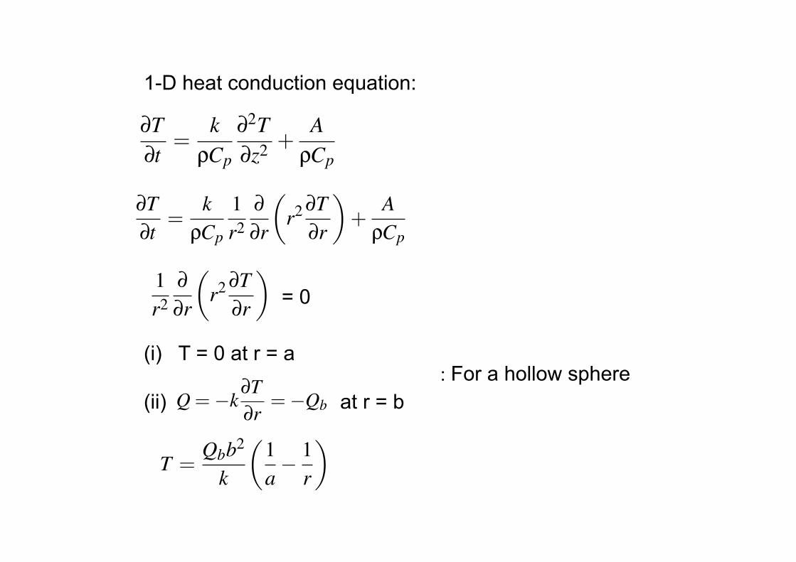
1-D heat conduction equation: ∂T
∂z
=∂∂z
T0er f
✓z
2p
kt
◆�=
T0ppkt
e
�z
2/4kt
∂T
∂t
=k
rC
p
1r
2∂∂r
✓r
2 ∂T
∂r
◆+
A
rC
p
4
∂T
∂z
=∂∂z
T0er f
✓z
2p
kt
◆�=
T0ppkt
e
�z
2/4kt
∂T
∂t
=k
rC
p
1r
2∂∂r
✓r
2 ∂T
∂r
◆+
A
rC
p
4
= 0
(i) T = 0 at r = a
(ii) at r = b
Q(z) =�k
∂T
∂z
∂T
∂t
=k
rC
p
—2T +
A
rC
p
∂T
∂t
=k
rC
p
—2T +
A
rC
p
�u ·—T
∂2T
∂z
2 =�A
k
Q =�k
∂T
∂r
=�Q
b
T =� A
2k
z
2 +(Q
d
+Ad)
k
z
er f (x) =2pp
Zx
0e
�y
2dy
er f c(x) =2pp
Z •
x
e
�y
2dy
d
dx
er f (x) =2pp
e
�x
2
3
d
dx
er f (x) =2pp
e
�x
2
∂T
∂z
=∂∂z
T
0
er f
✓z
2
pkt
◆�=
T
0ppkt
e
�z
2/4kt
∂T
∂t
=k
rC
p
1
r
2
∂∂r
✓r
2
∂T
∂r
◆+
A
rC
p
T =A
6k
(a2 � r
2)
�k
dT
dr
=Ar
3
T =Q
b
b
2
k
✓1
a
� 1
r
◆
0 =k
r
2
∂∂r
✓r
2
∂T
∂r
◆+A
T = T
a
✓z
L
+•
Ân=1
2
npsin
✓npz
L
◆exp
✓�n
2p2kt
L
2
◆◆
Re =rud
h⇠ 10
�19 �10
�21
4
: For a hollow sphere

∂T
∂z
=∂∂z
T0er f
✓z
2p
kt
◆�=
T0ppkt
e
�z
2/4kt
∂T
∂t
=k
rC
p
1r
2∂∂r
✓r
2 ∂T
∂r
◆+
A
rC
p
T =A
6k
(a2 � r
2)
4
T ≈ 63700 oC T ≈ 7000 oC
∂T
∂z
=∂∂z
T0er f
✓z
2p
kt
◆�=
T0ppkt
e
�z
2/4kt
∂T
∂t
=k
rC
p
1r
2∂∂r
✓r
2 ∂T
∂r
◆+
A
rC
p
4
∂T
∂z
=∂∂z
T0er f
✓z
2p
kt
◆�=
T0ppkt
e
�z
2/4kt
∂T
∂t
=k
rC
p
1r
2∂∂r
✓r
2 ∂T
∂r
◆+
A
rC
p
T =A
6k
(a2 � r
2)
�k
dT
dr
=Ar
3
T =�Q
b
b
2
k
✓1a
� 1r
◆
0 =k
r
2∂∂r
✓r
2 ∂T
∂r
◆+A
4
(i) T = 0 at r = a
(ii) T finite at r = 0
∂T
∂z
=∂∂z
T0er f
✓z
2p
kt
◆�=
T0ppkt
e
�z
2/4kt
∂T
∂t
=k
rC
p
1r
2∂∂r
✓r
2 ∂T
∂r
◆+
A
rC
p
T =A
6k
(a2 � r
2)
�k
dT
dr
=Ar
3
T =�Q
b
b
2
k
✓1a
� 1r
◆
0 =k
r
2∂∂r
✓r
2 ∂T
∂r
◆+A
4
= 80 X 10-3 W m-2
a = 6370 km; k = 4 Wm-1oC-1
∂T
∂z
=∂∂z
T0er f
✓z
2p
kt
◆�=
T0ppkt
e
�z
2/4kt
∂T
∂t
=k
rC
p
1r
2∂∂r
✓r
2 ∂T
∂r
◆+
A
rC
p
T =A
6k
(a2 � r
2)
�k
dT
dr
=Ar
3
T =�Q
b
b
2
k
✓1a
� 1r
◆
0 =k
r
2∂∂r
✓r
2 ∂T
∂r
◆+A
4
a


