UNIVERSITE LOUIS PASTEUR
ECOLE NATIONALE SUPERIEURE DE PHYSIQUE DE STRASBOURG
LABORATOIRE DES SYSTEMES PHOTONIQUES
THESE
presentee pour obtenir
le titre de Docteur de L’Universite Louis Pasteur
Discipline: Physique et Photonique
par
Katrin SCHMITT
Date de soutenance: 29 Juin 2006
UN NOUVEAU DISPOSITIF INTERFEROMETRIQUE POUR
LA DETECTION DE BIOMOLECULES SANS ADJUVANT
Directeur de these P. MEYRUEIS
Co-Directeur de these A. BRANDENBURG
Rapporteur interne J. FONTAINE
Rapporteur externe E. WAGNER
Rapporteur externe P. LAMBECK


UNIVERSITE LOUIS PASTEUR
ECOLE NATIONALE SUPERIEURE DE PHYSIQUE DE STRASBOURG
LABORATOIRE DES SYSTEMES PHOTONIQUES
THESIS
presented to obtain the
Doctorate Degree in the Louis Pasteur University of Strasbourg
in Physics
by
Katrin SCHMITT
A NEW WAVEGUIDE INTERFEROMETER FOR THE
LABEL FREE DETECTION OF BIOMOLECULES
June, 29th 2006 before the doctoral committee:
Thesis supervisor P. MEYRUEIS
Co-supervisor A. BRANDENBURG
Rapporteur J. FONTAINE
Rapporteur E. WAGNER
Rapporteur P. LAMBECK

Acknowledgements
Hereby I like to express my great gratitude to everyone who made this work possible.
I am deeply grateful to Prof. Patrick Meyrueis from the LSP in Strasbourg and to PD
Dr. Albrecht Brandenburg from the IPM in Freiburg for assuming the supervision of this
thesis as part of a joint project and for their unrestricted guidance and support. I also
thank Prof. Elmar Wagner, Prof. Joel Fontaine and Prof. Paul Lambeck for their interest
in this work and for their support in completing this dissertation.
I also like to thank Dr. Christian Hoffmann and Dr. Bernd Schirmer from the IPM for their
aid and support wherever needed during my thesis work and all their helpful discussions.
In particular for the final editing of this dissertation, I am indebted to Christian for his
detailed corrections that have greatly helped to improve this document.
At the IPM, I would like to thank all the colleagues, especially the bioanalytics group
and the OSS department, for the pleasant working atmosphere and their aid and support
for the project. I also like to thank Alfred Huber, Karl Kulmus, Heinrich Schulte and
Joachim Fuss for constructing the instruments and their aid in assembling, Monika Stefan
for her help in the clean room, and Nicole Ebentheuer and Peter Oswald for carrying out
some of the test measurements and their contributing in the nice lab atmosphere.
Further I like to thank the following persons for test measurement collaborations:
Dr. Kristian Muller from the Biological Institute of the University of Freiburg for making
the BIACORE 1000 available to us and Dr. Steffen Hartmann from Novartis, Basel for his
support during our measurement campaign with the BIACORE 2000. I also like to thank
Unaxis Optics in Liechtenstein for supplying the waveguide chips and Dr. Jorg Kraus and
Dr. Bernd Maisenholder for the supportive and friendly cooperation.
Finally I am deeply grateful for the love and support from my family. They have always
supported my decisions, no matter what. Most importantly, I like to thank Sebastian for
sharing many joyful years with me and all his help and patience in completing this work.
v


Resume
Le developpement rapide des sciences et technologies de la vie necessite de nouvelles
methodes et de nouveaux dispositifs miniaturises pour l’analyse des interactions biomolecu-
laires. Les systemes optiques de detection de biomolecules bases sur la detection de champs
evanescents pour l’analyse de liaisons biomoleculaires font l’objet d’un accroissement
rapide de leurs applications en matiere de diagnostic, monitoring de soins, developpement
de nouveaux medicaments. Pour etre efficace un nouveau biocapteur photonique doit etre
un instrument a haute sensibilite, precis et fiable, tout en etant adapte ou adaptable a un
large spectre d’application.
Dans le chapitre 1, nous precisons nos objectifs : proposer un microdispositif original a
haute sensibilite de type biochip, operant sans adjuvant exploitant le principe d’un micro
interferometre de Young. Nous decrivons l’architecture, le fondement technologique, et la
necessaire caracterisation theorique et experimentale du dispositif cible.
Dans le chapitre 2 nous presentons les bases theoriques que nous avons exploitees pour
developper le microsysteme cible particulierement la propagation de la lumiere dans
les guides d’onde planaires. Un resume des points essentiels concernant les biocap-
teurs est ensuite introduit en le completant par une presentation des methodes de calcul
d’optimisation que nous proposons d’utiliser. Une partie de ce chapitre est donc devolue
aux bases des methodes interferometriques que nous avons mises en œuvre. Une autre par-
tie concerne le traitement du signal, nous rappelons le principe du traitement de Fourier
rapide et la methode que nous avons selectionnee pour sa mise en œuvre. Nous intro-
duisons ensuite le processus d’implementation de cette methode du traitement du signal
concernant notamment des reductions du bruit par filtrage.
Le chapitre 3 est dedie aux considerations theoriques ayant trait aux connaissances en
biochimie necessaires pour la fonctionnalisation des effets biophotoniques. Nous traitons
ensuite de la theorie cinetique des interactions biochimiques comme les reactions anticorps-
antigenes. Les mises en liaisons sont decrites en detail en preparant ainsi les mesures de
validations decrites au chapitre 5. Une introduction est ensuite donnee a la strategie de
mesure experimentale que nous avons retenue.
L’architecture finale du biocapteur interferometrique que nous proposons est presentee
dans le chapitre 3 avec 2 variantes : un systeme a debit a deux canaux d’ecoulement et
une systeme statique MTP (microtiterplate). Le choix de l’architecture et des composants
selectionnes sont justifies en detail. Nous en faisons de meme pour la methode d’analyse
vii
viii
et de discussion des performances. Il en resulte un certain nombre de conclusions qui
nous permettent d’etablir le choix definitif du materiau substrat de la source de lumiere
et du detecteur. Nous exposons comment nous avons optimise l’architecture finale a par-
tir de l’analyse des consequences des differents choix que nous avons eu a effectuer, pour
obtenir des performances globalement optimales. Des complements de caracterisation
par des tests refractometriques sont ensuite decrits. Ce qui nous permet d’acceder a une
comparaison pertinente entre les resultats theoriques et experimentaux. Nous avons ainsi
obtenu une resolution en indice de 6 · 10−8 dans le cas des ecoulements dynamiques avec
un taux d’echantillonnage de 1 Hz. Cette resolution a ete ensuite amelioree en intro-
duisant un nouveau CCD. Nous avons pu en deduire que en ce cas le facteur limitant est
en fait le CCD en ce qui concerne le bruit de phase. Le bruit de phase est par contre egal
pour les 3 sources de lumiere testees. Ces sources peuvent donc tre exclues comme orig-
ines majoritaires de bruit de phase. Nous completons notre optimisation par l’adjonction
de filtres dont nous discutons le processus d’exploitation. La sensibilite experimentale
globale est ainsi en pleine accordance avec la simulation. La stabilite est excellente avec
une derive inferieure a 10−6 par heure. Nous decrivons ensuite le montage de qualifica-
tion pour le cas MTP avec 8 cellules. Nous justifions les choix technologiques en ce cas.
Nous qualifions ensuite les resultats experimentaux. Nous utilisons de l’ethanol pour les
tests refractometriques et nous obtenons une resolution en indice de 1.2 · 10−6 et 4.5 · 10−7
pour les modes TE et TM avec un echantillonnage a 1 Hz. Dans ce cas le CCD est aussi
le composant limitant mais il faut lui associer comme source significative de perturba-
tion une derive de la repetabilite des valeurs enregistrees. La stabilite de la reponse par
contre est inferieure a 5 · 10−5 par heure. Dans le chapitre 5 nous presentons une vali-
dation operationnelle des micro dispositifs que nous avons concus et realises sur un cas
biologique effectif. Nous discutons les resultats dans les 2 cas : statique et dynamique.
Nous decrivons la procedure de test. Differents effets de surface sont caracterises par
la mesure de l’angle de contact. Nous comparons les resultats a ceux existants dans le
litterature. Nous y ajoutons des experimentations avec des effets fluorescents pour opti-
miser la caracterisation de differentes modifications de la surface que nous avons testees
pour obtenir les fonctionnalites les plus robustes. La proteine G - IgG est enfin testee
dans les cas statiques et dynamique. Tous ces resultats sont egalement conformes a ceux
publies dans la litterature. Nous pouvons meme proceder avec nos micro dispositifs a une
evaluation de la cinetique qui est aussi conforme aux donnees provenant de la litterature.
Nous validons ensuite la detection de la proteine G par la proteine A. Les tests sont
poursuivis sur cytochrome c biotinyle sur une surface sensibilisee a la streptavidine. Une
comparaison avec les resultats obtenus avec un systeme commercialise valide la conformite
des fonctions implementees par rapport aux objectifs. Dans le cas de validation que nous
avons retenu, nous prouvons donc que notre micro systeme biophotonique donne des
resultats equivalents a un des meilleurs systemes commerciaux disponibles mais avec une
bien plus grande simplicite d’utilisation et avec un encombrement tres faible.

ix
Dans le chapitre 6 nous faisons un bilan de notre travail theorique et experimental en rap-
pelant les points principaux de nos aboutissements de facon synthetique. Nous concluons
par quelques elements de prospective concernant les evolutions futures des concepts de la
methode et de la technologie que nous avons proposee.

Summary
The rapid development in life science research requires continually new methods for the
analysis of biomolecular interactions. Optical detection systems based on evanescent field
sensing for biomolecular binding studies are marked by a fast increase of their applications
in fields like diagnostics, health care, screening or assay development. For a successful
implementation the optical biosensors need to be highly sensitive, selective and accurate
while allowing a wide range of applications. In this thesis we present a highly sensitive
label-free detection method based on the optical principle of a Young interferometer and
describe the design and realization of the system including an experimental characteriza-
tion and a validation of the biosensor system by application measurements.
In chapter 2, the theoretical basis of the propagation of light in planar waveguides and a
background of evanescent field sensors is provided as well as calculations concerning the
optimization of waveguide sensitivity for the interferometric biosensor proposed in this
thesis. One section is devoted to the theoretical basis of interferometry, especially the
optical principle of the Young interferometer since the proposed design for the interfero-
metric biosensor is based on the Young configuration. For signal evaluation, algorithms
based on Fast Fourier Transform are described and the implementation in the biosensor
system proposed along with system principles and relationships and signal filtering meth-
ods for noise reduction.
Chapter 3 is devoted to theoretical considerations on the biochemistry for waveguide sur-
face functionalization. The kinetic theory of biochemical interactions such as antibody-
antigen binding events is described in detail with respect to the evaluation of the ap-
plication measurements in chapter 5. Furthermore a biochemical background on the
application measurement reagents is given.
The design of the interferometric biosensor is presented in chapter 4, describing two dif-
ferent readout schemes: a flow-cell system implementing a two-channel flow cell as fluidic
element, and a system setup designed for the readout of microtiterplate (MTP)-formatted
wellplates. The system components and system designs of the interferometric biosensor
and their performance are discussed in detail. From the analysis of system components
several conclusions can be made, such as the choice of waveguide chip materials, the light
source and the CCD detector. The characteristics of the chosen components influence
the final design and setup, leading to an optimal set of parameters for the interferometric
biosensor. Further a detailed system characterization by refractometric test measurements
xi

xii
is provided including an evaluation of the experimental results compared to theoretical
calculations and simulations. Initial refractometric test measurements on the flow-cell
system with glycerin show an effective refractive index resolution of ≈ 6.0 · 10−8, corre-
sponding to a refractive index resolution of ≈ 7.5 · 10−7 for TE mode and ≈ 2.7 · 10−7 for
TM mode, respectively, at a sampling rate of 1 Hz. It is also found that the CCD sensor
is the limiting system component concerning phase noise, whereas the phase noise is ap-
proximately equal for all three light sources tested and therefore the light source can be
excluded as limiting factor. Signal filtering methods such as average filters are described
and analyzed concerning their suitability for phase noise reduction.
The experimentally derived sensitivity constants of the interferometer system are in very
good accordance with the theoretical values derived from waveguide theory in chapter 2.
The flow-cell system shows a good long-term stability with a typical drift of < 1 · 10−6/h
in ∆neff .
This chapter also presents the system design and describes the realized setup of the inter-
ferometric biosensor with an MTP-formatted 8-well frame as fluidic element and newly
introduced system components that are different from the flow cell system are discussed.
Suitable system components are chosen for an optimal set of design parameters for the
interferometric biosensor. The proposed biosensor system is characterized by refractomet-
ric test measurements with ethanol solutions and the experimental results are evaluated
and compared to theory and the results obtained with the flow cell system. The refrac-
tometric test measurements on the microplate system show an effective refractive index
resolution of ≈ 1.0 · 10−7, corresponding to a refractive index resolution of ≈ 1.2 · 10−6
for TE mode and ≈ 4.5 · 10−7 for TM mode, respectively, at a sampling rate of 1 Hz. We
found that, apart from the CCD sensor being the limiting system component concerning
phase noise, the resolution of the microplate system is finally limited by the repeatability
of the recorded data values.
The experimentally derived sensitivity constants of the microplate interferometer system
are also in good accordance with the theoretical values derived from waveguide theory in
chapter 2. The system shows a long-term stability with a typical drift of < 5 · 10−5/h in
∆neff and a repeatability of < 2 · 10−7 in ∆neff .
Chapter 5 presents a validation of the interferometric biosensor by biological application
measurements on both systems and their discussion. In this chapter a detailed description
of the materials and methods used for application and test measurements, a character-
ization of the surface chemistry on the Ta2O5 waveguide chips and finally application
measurements on different affinity systems is provided. Differently functionalized sur-
faces are characterized by contact angle measurements and compared to literature values.
Experiments with fluorescently labeled streptavidin allow a detailed characterization of
different surface modifications and a direct comparison to measurements with the inter-
ferometric biosensor with the aim to find a stable and robust surface functionalization for
the immobilization of biotinylated reagents.

xiii
The immunoassay protein G - IgG is tested on the flow-cell system as well as on the mi-
croplate system, yielding affinity rate constants that are in good agreement with values
found in literature. Experimental data obtained with the two-channel flow-cell system
allow an evaluation of the reaction kinetics, while the microplate system is suited for
the parallel detection of several analyte concentrations. Furthermore the direct detection
of IgG by immobilized protein A is shown and the affinity rate constants determined.
Test measurements with biotinylated cytochrome c on a streptavidin-functionalized sur-
face compared directly to the same assay performed on the commercial biosensor system
BIACORE 1000 show the suitability of the developed surface chemistry for the Ta2O5
waveguide chips implemented in the interferometric biosensor.
The interferometric biosensor has been successfully used for the detection of the affinity
system α-NPT IgG - E2-NPT developed at Novartis in Basel. We tested the assay on both
the interferometric biosensor (flow-cell system) and the commercial BIACORE 2000 sys-
tem provided by Novartis. A comparison of the surface chemistries used on both biosensor
systems is presented, and a series of measurements to detect the analyte from different
sample buffers. We found that the performance of the interferometric biosensor system
proposed in this thesis is approximately equal to the BIACORE system with a detection
limit for the analyte in the low picomolar range. Measurements in cell lysate as sample
matrix show that with the interferometric biosensor the analyte can be detected even out
of a complex sample matrix without significant unspecific binding.
In chapter 6, conclusions concerning the development of the interferometric biosensor and
the results from the experimental characterization and validation are presented. A com-
parison between the proposed interferometric biosensor and other label-free biosensors is
given. The chapter concludes with an outlook concerning further improvements of the
resolution and surface chemistry and further possibilities for developments to adapt the
sensor design to high throughput applications.

xiv

Contents
Acknowledgements v
Resume vii
Summary xi
Table of Contents xvii
List of Figures xxii
List of Tables xxiii
Abbreviations xxv
1 Introduction 1
1.1 General introduction . . . . . . . . . . . . . . . . . . . . . . . . . . . . . . 1
1.2 Label-free biosensors . . . . . . . . . . . . . . . . . . . . . . . . . . . . . . 2
1.3 Aim of the Thesis . . . . . . . . . . . . . . . . . . . . . . . . . . . . . . . . 4
2 Theoretical background in optics 7
2.1 Introduction . . . . . . . . . . . . . . . . . . . . . . . . . . . . . . . . . . . 7
2.2 Refraction and reflection in ray optics . . . . . . . . . . . . . . . . . . . . . 8
2.3 Electromagnetic theory of planar waveguides . . . . . . . . . . . . . . . . . 11
2.3.1 Maxwell’s equations . . . . . . . . . . . . . . . . . . . . . . . . . . 11
2.3.2 Wave equations for planar waveguides . . . . . . . . . . . . . . . . . 12
2.3.3 Modes of a planar waveguide . . . . . . . . . . . . . . . . . . . . . . 13
2.4 Evanescent field sensors . . . . . . . . . . . . . . . . . . . . . . . . . . . . 17
2.4.1 Sensitivity to cover refractive index changes ∆nc . . . . . . . . . . . 18
2.4.2 Sensitivity to adlayer formation . . . . . . . . . . . . . . . . . . . . 20
2.4.3 Molecule adsorption and binding . . . . . . . . . . . . . . . . . . . 21
2.5 Interferometry . . . . . . . . . . . . . . . . . . . . . . . . . . . . . . . . . . 22
2.5.1 Diffraction and interference . . . . . . . . . . . . . . . . . . . . . . 22
2.5.2 Young’s interferometer . . . . . . . . . . . . . . . . . . . . . . . . . 26
xv

xvi CONTENTS
2.5.3 Influence of coherence length . . . . . . . . . . . . . . . . . . . . . . 27
2.6 Fourier transform analysis for signal processing . . . . . . . . . . . . . . . 30
2.7 Signal analysis and processing . . . . . . . . . . . . . . . . . . . . . . . . . 34
2.7.1 System principles and relationships . . . . . . . . . . . . . . . . . . 34
2.7.2 Noise sources and distortion effects . . . . . . . . . . . . . . . . . . 35
2.7.3 Signal filtering methods . . . . . . . . . . . . . . . . . . . . . . . . 38
3 Theoretical background in biochemistry 41
3.1 Introduction . . . . . . . . . . . . . . . . . . . . . . . . . . . . . . . . . . . 41
3.2 Immunoassays . . . . . . . . . . . . . . . . . . . . . . . . . . . . . . . . . . 41
3.3 Surface chemistry . . . . . . . . . . . . . . . . . . . . . . . . . . . . . . . . 43
3.4 Kinetics of binding reactions . . . . . . . . . . . . . . . . . . . . . . . . . . 45
3.4.1 The 1:1 interaction model . . . . . . . . . . . . . . . . . . . . . . . 45
3.4.2 Evaluation of non-equilibrium kinetic data . . . . . . . . . . . . . . 48
3.4.3 Influences of mass transport on kinetic data . . . . . . . . . . . . . 49
3.5 Biochemical background on the application measurement reagents . . . . . 50
3.5.1 Immunoreactands Immunoglobulin G - Protein G or A . . . . . . . 50
3.5.2 Affinity system biotin - streptavidin . . . . . . . . . . . . . . . . . . 52
3.5.3 Cytochrome c . . . . . . . . . . . . . . . . . . . . . . . . . . . . . . 55
4 Sensor design and characterization 57
4.1 Introduction . . . . . . . . . . . . . . . . . . . . . . . . . . . . . . . . . . . 57
4.1.1 Requirements for the interferometric biosensor system . . . . . . . . 58
4.2 Interferometric biosensor: flow cell system . . . . . . . . . . . . . . . . . . 59
4.2.1 Biosensor setup - components . . . . . . . . . . . . . . . . . . . . . 59
4.2.2 Biosensor setup - realization . . . . . . . . . . . . . . . . . . . . . . 68
4.2.3 Experimental characterization of the components . . . . . . . . . . 70
4.2.4 Signal analysis and processing . . . . . . . . . . . . . . . . . . . . . 80
4.2.5 Experimental characterization of the biosensor system . . . . . . . . 86
4.2.6 Conclusion . . . . . . . . . . . . . . . . . . . . . . . . . . . . . . . . 93
4.3 Interferometric biosensor: microplate system . . . . . . . . . . . . . . . . . 94
4.3.1 Introduction . . . . . . . . . . . . . . . . . . . . . . . . . . . . . . . 94
4.3.2 Biosensor setup - components . . . . . . . . . . . . . . . . . . . . . 95
4.3.3 Biosensor setup - realization . . . . . . . . . . . . . . . . . . . . . . 98
4.3.4 Signal analysis and processing . . . . . . . . . . . . . . . . . . . . . 101
4.3.5 Simulation algorithm for signal analysis . . . . . . . . . . . . . . . . 104
4.3.6 Experimental characterization of the biosensor system . . . . . . . . 104
4.3.7 Conclusion . . . . . . . . . . . . . . . . . . . . . . . . . . . . . . . . 109

xvii
5 Application measurements 111
5.1 Introduction . . . . . . . . . . . . . . . . . . . . . . . . . . . . . . . . . . . 111
5.2 Materials and methods . . . . . . . . . . . . . . . . . . . . . . . . . . . . . 111
5.2.1 Materials . . . . . . . . . . . . . . . . . . . . . . . . . . . . . . . . 111
5.2.2 Methods . . . . . . . . . . . . . . . . . . . . . . . . . . . . . . . . . 115
5.3 Characterization of the surface chemistry . . . . . . . . . . . . . . . . . . . 119
5.3.1 Contact angle measurements . . . . . . . . . . . . . . . . . . . . . . 119
5.3.2 Binding of fluorescently labeled streptavidin . . . . . . . . . . . . . 121
5.4 Affinity system biotin-streptavidin . . . . . . . . . . . . . . . . . . . . . . . 125
5.5 Immunoreaction Protein G-Immunoglobulin G . . . . . . . . . . . . . . . . 129
5.5.1 Flow cell system: kinetic analysis . . . . . . . . . . . . . . . . . . . 129
5.5.2 Microplate system: parallel detection . . . . . . . . . . . . . . . . . 133
5.6 Immunoreaction Protein A-Immunoglobulin G . . . . . . . . . . . . . . . . 135
5.7 Biotinylated Cytochrome c:
Comparison with BIACORE 1000 technology . . . . . . . . . . . . . . . . 137
5.8 Biotinylated α-NPT IgG antigen:
Comparison with BIACORE 2000 technology . . . . . . . . . . . . . . . . 140
5.8.1 Measurements in PBS-BSA as sample matrix . . . . . . . . . . . . 142
5.8.2 Measurements in cell lysate as sample matrix . . . . . . . . . . . . 146
5.9 Conclusion . . . . . . . . . . . . . . . . . . . . . . . . . . . . . . . . . . . . 150
6 Conclusions and Outlook 153
6.1 Summary of the results . . . . . . . . . . . . . . . . . . . . . . . . . . . . . 153
6.2 Discussion . . . . . . . . . . . . . . . . . . . . . . . . . . . . . . . . . . . . 156
6.3 Outlook . . . . . . . . . . . . . . . . . . . . . . . . . . . . . . . . . . . . . 157
Appendix 159
Bibliography 175
Publications 183
Vita 185

xviii

List of Figures
2.1 Cross-section of a planar waveguide . . . . . . . . . . . . . . . . . . . . . . 7
2.2 Refraction and reflection at a planar interface . . . . . . . . . . . . . . . . 8
2.3 Total internal reflection in a planar waveguide . . . . . . . . . . . . . . . . 10
2.4 Field distribution for planar waveguide . . . . . . . . . . . . . . . . . . . . 15
2.5 TE-mode diagram . . . . . . . . . . . . . . . . . . . . . . . . . . . . . . . . 16
2.6 TM-mode diagram . . . . . . . . . . . . . . . . . . . . . . . . . . . . . . . 16
2.7 Evanescent field sensing . . . . . . . . . . . . . . . . . . . . . . . . . . . . 18
2.8 Theoretical sensitivity of a waveguide to cover refractive index changes . . 19
2.9 Theoretical sensitivity of a waveguide to surface adlayer changes . . . . . . 20
2.10 Light fringes from single and double slit diffraction . . . . . . . . . . . . . 24
2.11 Fraunhofer diffraction at a single slit . . . . . . . . . . . . . . . . . . . . . 25
2.12 Fraunhofer diffraction at a double slit . . . . . . . . . . . . . . . . . . . . . 26
2.13 Young’s double slit configuration . . . . . . . . . . . . . . . . . . . . . . . 27
2.14 Interference of partially coherent light . . . . . . . . . . . . . . . . . . . . . 28
2.15 Intensity distribution produced by quasi-monochromatic light . . . . . . . 29
2.16 Far-field interference pattern of differently coherent light source, simulated 30
2.17 Flow chart of a block average filter . . . . . . . . . . . . . . . . . . . . . . 39
2.18 Flow chart of a moving average filter . . . . . . . . . . . . . . . . . . . . . 40
3.1 One-step immunoassay . . . . . . . . . . . . . . . . . . . . . . . . . . . . . 42
3.2 Multi-step immunoassay . . . . . . . . . . . . . . . . . . . . . . . . . . . . 42
3.3 Chemical formulas for GOPS and ATPS . . . . . . . . . . . . . . . . . . . 44
3.4 Dose-response curve . . . . . . . . . . . . . . . . . . . . . . . . . . . . . . . 47
3.5 Comparison of binding data for different time intervals . . . . . . . . . . . 48
3.6 Illustration of ideal binding curves . . . . . . . . . . . . . . . . . . . . . . . 49
3.7 Schematic structure of an IgG antibody . . . . . . . . . . . . . . . . . . . . 51
3.8 Stick model of a human immunoglobulin G antibody . . . . . . . . . . . . 52
3.9 Stick model of a streptavidin-biotin complex . . . . . . . . . . . . . . . . . 53
3.10 Chemical structure of NHS-LC-biotin . . . . . . . . . . . . . . . . . . . . . 54
3.11 Reaction NHS-biotin with amine-modified surface . . . . . . . . . . . . . . 54
3.12 Three-dimensional model of cytochrome c . . . . . . . . . . . . . . . . . . 55
xix

xx LIST OF FIGURES
4.1 Schematic design of the interferometric biosensor . . . . . . . . . . . . . . 58
4.2 Beam profile of the SLD . . . . . . . . . . . . . . . . . . . . . . . . . . . . 61
4.3 CAD drawing of the chip mount . . . . . . . . . . . . . . . . . . . . . . . . 62
4.4 Photograph of the chip mount . . . . . . . . . . . . . . . . . . . . . . . . . 62
4.5 Double slit design . . . . . . . . . . . . . . . . . . . . . . . . . . . . . . . . 63
4.6 Waveguide chip design and dimensions . . . . . . . . . . . . . . . . . . . . 64
4.7 Refractive index profile and field distribution . . . . . . . . . . . . . . . . . 65
4.8 AFM picture of diffraction grating . . . . . . . . . . . . . . . . . . . . . . . 66
4.9 Two-channel flow cell and flow cell mount . . . . . . . . . . . . . . . . . . 67
4.10 Single-channel flow cell and its casting mold . . . . . . . . . . . . . . . . . 67
4.11 Functional design of the interferometric biosensor IBS 201 . . . . . . . . . . 69
4.12 Photograph of the interferometric biosensor IBS 201 . . . . . . . . . . . . . 69
4.13 Light-current characteristics of the SLD . . . . . . . . . . . . . . . . . . . . 70
4.14 Wavelength-current and wavelength-resistance characteristics of the SLD . 71
4.15 Interferogram recorded with the SLD in TM mode . . . . . . . . . . . . . . 72
4.16 Light-current characteristics of the laser diode . . . . . . . . . . . . . . . . 73
4.17 Dark current measurement of CCD sensors . . . . . . . . . . . . . . . . . . 75
4.18 Signal-to-noise of CCD sensors . . . . . . . . . . . . . . . . . . . . . . . . . 76
4.19 Correlation of phase noise and pixel noise . . . . . . . . . . . . . . . . . . . 77
4.20 Setup for coupling angle experiment and measurement result . . . . . . . . 78
4.21 Coupling angle tolerances for different focal lengths . . . . . . . . . . . . . 79
4.22 Transmission intensities for input and output coupling in TE mode . . . . 79
4.23 Comparison of coupling efficiencies for TE and TM mode . . . . . . . . . . 80
4.24 Interferogram recorded by the CCD camera and the region of interest . . . 81
4.25 FFT Plot . . . . . . . . . . . . . . . . . . . . . . . . . . . . . . . . . . . . 82
4.26 Influence of zeropadding on FFT signal peak . . . . . . . . . . . . . . . . . 83
4.27 Influence of zeropadding on phase trend . . . . . . . . . . . . . . . . . . . 84
4.28 Reduction of phase noise by averaging . . . . . . . . . . . . . . . . . . . . 85
4.29 Refractive index measurement with SLD in TE mode . . . . . . . . . . . . 87
4.30 Calibration curve for TE mode . . . . . . . . . . . . . . . . . . . . . . . . 87
4.31 Refractive index measurement with SLD in TM mode . . . . . . . . . . . . 88
4.32 Calibration curve for TM mode . . . . . . . . . . . . . . . . . . . . . . . . 89
4.33 Autocorrelation of a measurement baseline . . . . . . . . . . . . . . . . . . 90
4.34 Comparison of CCD sensors, baseline noise . . . . . . . . . . . . . . . . . . 90
4.35 Phase noise reduction by signal averaging . . . . . . . . . . . . . . . . . . . 91
4.36 Non-random signal distortion . . . . . . . . . . . . . . . . . . . . . . . . . 91
4.37 Influence of light source instability on signal noise . . . . . . . . . . . . . . 92
4.38 Reader options . . . . . . . . . . . . . . . . . . . . . . . . . . . . . . . . . 94
4.39 Microplate layout options . . . . . . . . . . . . . . . . . . . . . . . . . . . 95
4.40 Design of the IBS 801 optics mount . . . . . . . . . . . . . . . . . . . . . . 97
LIST OF FIGURES xxi
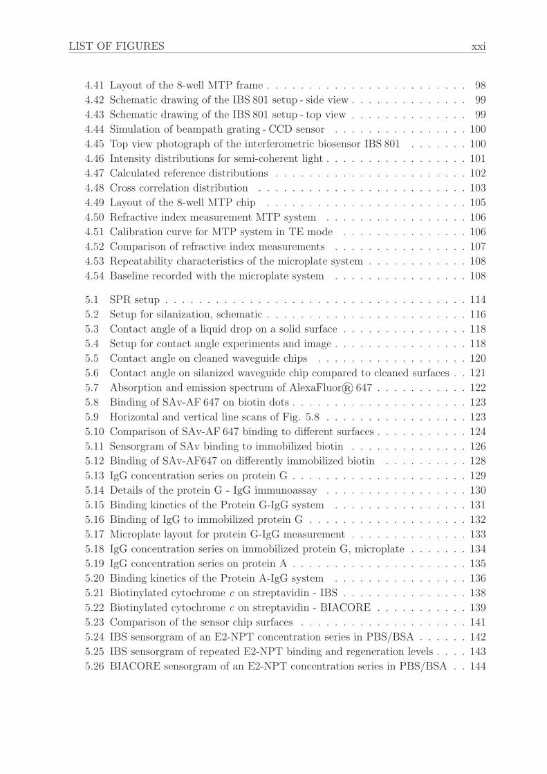
4.41 Layout of the 8-well MTP frame . . . . . . . . . . . . . . . . . . . . . . . . 98
4.42 Schematic drawing of the IBS 801 setup - side view . . . . . . . . . . . . . . 99
4.43 Schematic drawing of the IBS 801 setup - top view . . . . . . . . . . . . . . 99
4.44 Simulation of beampath grating - CCD sensor . . . . . . . . . . . . . . . . 100
4.45 Top view photograph of the interferometric biosensor IBS 801 . . . . . . . 100
4.46 Intensity distributions for semi-coherent light . . . . . . . . . . . . . . . . . 101
4.47 Calculated reference distributions . . . . . . . . . . . . . . . . . . . . . . . 102
4.48 Cross correlation distribution . . . . . . . . . . . . . . . . . . . . . . . . . 103
4.49 Layout of the 8-well MTP chip . . . . . . . . . . . . . . . . . . . . . . . . 105
4.50 Refractive index measurement MTP system . . . . . . . . . . . . . . . . . 106
4.51 Calibration curve for MTP system in TE mode . . . . . . . . . . . . . . . 106
4.52 Comparison of refractive index measurements . . . . . . . . . . . . . . . . 107
4.53 Repeatability characteristics of the microplate system . . . . . . . . . . . . 108
4.54 Baseline recorded with the microplate system . . . . . . . . . . . . . . . . 108
5.1 SPR setup . . . . . . . . . . . . . . . . . . . . . . . . . . . . . . . . . . . . 114
5.2 Setup for silanization, schematic . . . . . . . . . . . . . . . . . . . . . . . . 116
5.3 Contact angle of a liquid drop on a solid surface . . . . . . . . . . . . . . . 118
5.4 Setup for contact angle experiments and image . . . . . . . . . . . . . . . . 118
5.5 Contact angle on cleaned waveguide chips . . . . . . . . . . . . . . . . . . 120
5.6 Contact angle on silanized waveguide chip compared to cleaned surfaces . . 121
5.7 Absorption and emission spectrum of AlexaFluor® 647 . . . . . . . . . . . 122
5.8 Binding of SAv-AF 647 on biotin dots . . . . . . . . . . . . . . . . . . . . . 123
5.9 Horizontal and vertical line scans of Fig. 5.8 . . . . . . . . . . . . . . . . . 123
5.10 Comparison of SAv-AF 647 binding to different surfaces . . . . . . . . . . . 124
5.11 Sensorgram of SAv binding to immobilized biotin . . . . . . . . . . . . . . 126
5.12 Binding of SAv-AF647 on differently immobilized biotin . . . . . . . . . . 128
5.13 IgG concentration series on protein G . . . . . . . . . . . . . . . . . . . . . 129
5.14 Details of the protein G - IgG immunoassay . . . . . . . . . . . . . . . . . 130
5.15 Binding kinetics of the Protein G-IgG system . . . . . . . . . . . . . . . . 131
5.16 Binding of IgG to immobilized protein G . . . . . . . . . . . . . . . . . . . 132
5.17 Microplate layout for protein G-IgG measurement . . . . . . . . . . . . . . 133
5.18 IgG concentration series on immobilized protein G, microplate . . . . . . . 134
5.19 IgG concentration series on protein A . . . . . . . . . . . . . . . . . . . . . 135
5.20 Binding kinetics of the Protein A-IgG system . . . . . . . . . . . . . . . . 136
5.21 Biotinylated cytochrome c on streptavidin - IBS . . . . . . . . . . . . . . . 138
5.22 Biotinylated cytochrome c on streptavidin - BIACORE . . . . . . . . . . . 139
5.23 Comparison of the sensor chip surfaces . . . . . . . . . . . . . . . . . . . . 141
5.24 IBS sensorgram of an E2-NPT concentration series in PBS/BSA . . . . . . 142
5.25 IBS sensorgram of repeated E2-NPT binding and regeneration levels . . . . 143
5.26 BIACORE sensorgram of an E2-NPT concentration series in PBS/BSA . . 144

xxii LIST OF FIGURES
5.27 Langmuir fit of the α-NPT IgG - E2-NPT in PBS/BSA binding data . . . . 145
5.28 IBS sensorgram of an E2-NPT concentration series in E. coli lysate . . . . 147
5.29 IBS sensorgram of the E2-NPT concentration series in E. coli lysate, enlarged148
5.30 BIACORE sensorgram of an E2-NPT concentration series in E. coli lysate 149
5.31 Langmuir fit of the α-NPT IgG - E2-NPT (in lysate) binding data . . . . . 149
5.32 IBS sensorgram of the E2-NPT concentration series in E. coli lysate, one-
channel configuration . . . . . . . . . . . . . . . . . . . . . . . . . . . . . . 150
6.1 Refractive index table for ethanol . . . . . . . . . . . . . . . . . . . . . . . 165
6.2 Refractive index table for glycerin . . . . . . . . . . . . . . . . . . . . . . . 166
6.3 User interface for step motor control . . . . . . . . . . . . . . . . . . . . . 167
6.4 User interface for interferometer FFT algorithm . . . . . . . . . . . . . . . 168
6.5 Flowchart FFT algorithm . . . . . . . . . . . . . . . . . . . . . . . . . . . 169
6.6 Flowchart CC algorithm . . . . . . . . . . . . . . . . . . . . . . . . . . . . 170
6.7 User interface simulation algorithm . . . . . . . . . . . . . . . . . . . . . . 171
6.8 DLL of test function . . . . . . . . . . . . . . . . . . . . . . . . . . . . . . 172

List of Tables
4.1 Sample calculation for different double slits . . . . . . . . . . . . . . . . . . 64
4.2 Waveguide chip parameters . . . . . . . . . . . . . . . . . . . . . . . . . . 65
4.3 Comparison of CCD sensors . . . . . . . . . . . . . . . . . . . . . . . . . . 74
4.4 Coupling angles for TE and TM and different grating depths . . . . . . . . 78
5.1 Technical data of BIACORE instruments . . . . . . . . . . . . . . . . . . . 113
5.2 Cleaning procedures for waveguide chips . . . . . . . . . . . . . . . . . . . 115
5.3 Pretreatment and cleaning of chips for contact angle measurements . . . . 120
5.4 Comparison of SAv-AF 647 binding to different surfaces . . . . . . . . . . . 125
5.5 Binding constants for protein G-IgG and protein A-IgG . . . . . . . . . . . 137
5.6 Comparison IBS 201 and BIACORE 1000U . . . . . . . . . . . . . . . . . . 139
6.1 Summary of the properties of the interferometric biosensors . . . . . . . . . 154
6.2 Comparison of the interferometric biosensor with other label-free sensors . 156
xxiii

xxiv

Abbreviations
AFM Atomic force microscope
APTS 3-Aminopropyl-triethoxysilane
BSA Bovine serum albumin
CAD Computer Aided Design
DFT Discrete Fourier Transformation
DI De-ionized
DLL Dynamic link library
ELISA Enzyme-linked Immunosorbent Assay
FFT Fast Fourier Transformation
FT Fourier Transformation
FWHM Full Width at Half Maximum
GOPS 3-Glycidoxypropyl-triethoxysilane
HTS High throughput screening
IAD Ion assisted deposition
IgG Immunoglobulin G
kDa kiloDalton
LED Light emitting diode
MTP Microtiterplate
MZI Mach-Zehnder interferometer
PBS Phosphate buffered saline
RifS Reflectometric interference spectroscopy
SAM Self-assembled monolayer
SAv Streptavidin
SCM Spectral correlation method
SDS-PAGE Sodium Dodecyl Sulfate Polyacrylamide Gel Electrophoresis
SLD Superluminescent diode
SNR Signal-to-noise ratio
SPR Surface plasmon resonance
TE Transversal electric
TM Transversal magnetic
WIOS Wavelength interrogated optical sensor
YI Young interferometer
xxv

xxvi

Chapter 1
Introduction
1.1 General introduction
Today many scientists are working on the same goal: to unravel the secrets of life. Sev-
eral years after the completion of the human genome project the focus is now on another
molecular species in the human body: the proteins. The constellation of all proteins in a
cell is called proteome, and studies elucidating protein activity and function is named pro-
teomics, a fast growing research field that will become even more important in the future.
Proteomics has the potential to provide insights in structure, function and expression
data of proteins and thus is of great interest in areas like drug discovery, diagnosis, phar-
macological and toxicological studies.
Yet mapping the proteome is by far a more difficult and cost- and time-consuming task
than mapping the genome, so there is a need to think about efficient ways and tools to
help identifying the huge amount of different proteins in the body and their functions and
activities. In the last years improvements in technologies like two-dimensional gel elec-
trophoresis, mass spectrometry and the development of protein-based arrays and various
kinds of biosensors have contributed to manage this task (Hebestreit , 2001).
Another issue is the screening for new molecules, predominantly in pharmaceutical re-
search. Here it is important to detect even very small analyte molecules and get informa-
tion about their reactivity with a huge amount of different receptors such as antibodies,
1

2 CHAPTER 1 Introduction
which also demands efficient tools to recognize these various affinity systems by monitor-
ing several thousands of reactions every day. This research field is named high throughput
screening (HTS), and 100000 assays in a miniaturized format are anticipated to be soon
routine in laboratories (Hertzberg and Pope, 2000).
1.2 Label-free biosensors
In many cases, the molecule of interest is prepared with a label, such as fluorescent dyes,
radioactive markers, or colorimetric reactands. The most popular labeling method is us-
ing fluorescent markers that are nowadays available at almost each wavelength within the
visible spectrum of light, plus UV and near infrared. Established assay protocols and
sophisticated detection technology make the use of these dyes easy and convenient, but
also mean an additional step in the assay protocol for labeling. Furthermore, a certain
level of photobleaching and/or quenching when exposed to light is inherent to fluorescent
dyes, which is a drawback when quantitative information is needed. Also, a marker of any
kind attached to a biomolecule might alter its functionality, conformation, or reactivity
with its binding partner. In the worst case, a binding site gets occupied by the marker
molecule and the binding event is totally impeded, leading to false negatives. Another
disadvantage is a relatively high background signal that might give a false positive.
These facts, among the labeling step being cost- and time-consuming, have induced an
increasing demand for technologies allowing a label-free detection of biomolecular in-
teractions. One approach is the use of label-free biosensors. Biosensors are generally
considered to be a subgroup of chemosensors, consisting of a selective biological compo-
nent and a transducer (Ramsden, 1997; Cammann, 2000). This transducer transforms
physical changes due to the recognition of the biomolecule into an electrical signal. A
special kind of biosensor is the label-free optical biosensor. The first biosensors of this
type appeared in the 1980s with the expanded development of surface plasmon resonance
(SPR) and optical waveguide sensors (Cooper , 2002, 2003). Since then many other types
of label-free optical biosensors evolved with a growing range of applications. A review of
label-free optical biosensors can be found in (Leatherbarrow and Edwards, 1999) or (Baird

1.2 Label-free biosensors 3
and Myszka, 2001).
The most commonly found label-free biosensor in laboratories is probably the SPR sensor,
which relies on the detection of changes in the surface coverage within the evanescent field
(van der Merwe, 2005). The evanescent field is an exponentially decaying part of the light
of a guided mode found directly above (or below) the waveguide. In the case of SPR, a
glass substrate is coated with a thin gold film. When illuminated with light from a cer-
tain angle, a maximum of light intensity is transferred into the gold layer where oscillating
plasma waves (surface plasmons) are excited. Thus a minimum of light is reflected back
into the substrate. This angle is called the surface plasmon resonance angle. Any kind of
change in surface coverage on the gold film, caused by e.g. biomolecule binding, results
in a change of this angle, and these changes are constantly monitored and evaluated. The
optical setup and operation was first described by Kretschmann and Raether (1968).
Other label-free optical biosensors are for example the grating coupler (Bilitewski et al.,
1998; Lukosz et al., 1991; Polzius et al., 1997), narrow bandwidth guided-mode resonant
filter systems (Cunningham et al., 2002) or reflectometric interference spectroscopy (RifS)
(Kroger et al., 2002; Schutz , 2000). The grating coupler system consists of a waveguide
chip with etched gratings and can be configured either as input or as output grating cou-
pler and thus measures an incoupling or outcoupling angle, respectively, as a function of
changes in surface mass coverage in the evanescent field. The guided-mode resonant filter
system uses a sub-wavelength grating waveguide structure in a plastic substrate which
reflects only a very narrow band when illuminated with white light at normal incidence.
The resonantly reflected wavelength depends upon the surface optical density and thus
the detection phenomenon actually occurs within the waveguide and not in an evanescent
wave. This system has already been configured to work with up to 384 well microtiter-
plates (MTP) (Cunningham et al., 2004) as an efficient tool for HTS.
The third system mentioned above, RifS, is based on the spectral distribution of re-
flectance of thin films on a glass substrate when illuminated with white light. This
spectral pattern changes when the surface coverage is changing. The RifS system was
the first label-free system set up to read 96 well MTPs, also for HTS (Kroger et al.,
2002). Another wide-spread class of label-free optical biosensors is represented by vari-

4 CHAPTER 1 Introduction
ous interferometric systems, among them the Rayleigh interferometer (Chen et al., 2003),
Mach-Zehnder interferometer (Weisser et al., 1999), Hartmann interferometer (Schnei-
der et al., 1997, 2000) and Young interferometer setups (Brandenburg et al., 2000; Ymeti
et al., 2002; Cross et al., 2003). Other interferometric approaches include for example the
integrated-optical (IO) difference interferometer (Stamm et al., 1998) and the spectral
correlation method (Nikitin et al., 2003).
Theoretical estimations have compared the sensitivities of IO devices including interfero-
meters and surface plasmon resonance sensors (Lukosz , 1991); here IO interferometric
systems are predicted to have the highest sensitivity.
1.3 Aim of the Thesis
Among the various kinds of label free biosensors one approach for sensitive, label-free de-
tection of biomolecules is the interferometric detection implementing optical waveguides
as sensing elements, as proposed by Brandenburg (Brandenburg et al., 2000). In his work
a Young interferometer design based on a silicon oxinitride waveguide structure as beam
splitter and sensing element is proposed.
The main goal of this thesis is then to elaborate an interferometric system based on a
Young interferometer for the extremely sensitive detection of biomolecules which is suit-
able for high throughput biochemical and biological analysis. The core of this system is
a planar optical waveguide chip where gratings are used as light coupling elements. Un-
like the previous IO Young interferometer setup, where the waveguide chip combined the
interferometer itself and the sensing area, this design is free-spaced, i.e. the waveguide
chip operates solely as sensing element. Preliminary work on a two-channel prototype of
such an interferometric system (MacKenzie, 2003) has shown that this configuration is
efficient and suitable for various biological applications.
As a first step, the two-channel system is optimized in terms of signal-to-noise ratio and
system stability in order to perform highly sensitive and reproducible measurements. For
biological applications, appropriate surface chemistries are developed and tested. Differ-
ent biochemical assays are realized and the resulting system is experimentally compared

1.3 Aim of the Thesis 5
with competing technologies based on SPR.
In a second step, the existing system is redesigned to an MTP reading format for high
throughput analysis of biochemical interactions. The system setup is realized and test
measurements for calibration and characterization are performed. Subsequently simple
biological measurements show the suitability of this interferometer system for further use
in research and medical diagnosis or screening.
In chapter 2, the basic theory of planar waveguides and of the Fast Fourier transformation
for interferogram signal analysis is presented. Chapter 3 is devoted to theoretical consid-
erations on the biochemistry needed for waveguide surface functionalization, along with
the kinetic theory of biochemical interactions such as antibody-antigen binding events.
In chapter 4, the design of both the two-channel configuration and the MTP readout
interferometric system and their performance characteristics are discussed in detail. The
following chapter presents biological application measurements on both systems and their
discussion. Finally a general conclusion and an outlook are given in chapter 6.
This thesis is part of a joint project between the University of Strasbourg (ULP), France
and the Fraunhofer Institute for Physical Measurement Techniques (IPM) in Freiburg,
Germany. The project is part of the INTERREG IIIa-Rhenaphotonics project.


Chapter 2
Theoretical background in optics
2.1 Introduction
A brief overview on the theory of optical waveguides shall be given in this chapter to pro-
vide a background on our work. An optical waveguide, also known as dielectric waveguide,
is a structure that is able to confine and guide light. There exist various kinds of optical
waveguides, the most prominent probably being the optical fiber used in telecommunica-
tions. Integrated optics constitute another kind of optical waveguide. Here mostly planar
optical waveguides are of interest. Since in the interferometric biosensor described in this
thesis also a planar waveguide is used as sensing element, the theoretical considerations
given here will focus on this type of waveguide. A more comprehensive description of the
theory of optical waveguides can be found in (Kogelnik , 1988).
Figure 2.1: Cross-section of a planar waveguide. A medium of high refractive index nf is
surrounded by media with lower refractive indices nc and ns.
7

8 CHAPTER 2 Theoretical background in optics
In the simplest case of a planar waveguide a substrate is coated with a thin film (typically
with a thickness ranging from several hundred nanometers up to several hundred microm-
eters) of a high-refractive medium (ns < nf). The cover medium is air with nc < ns < nf .
In the following theoretical descriptions all the dielectric media are assumed to be ideal,
i.e. homogeneous, isotropic and loss-free.
2.2 Refraction and reflection in ray optics
We consider two ideal dielectric media with refractive indices n1 and n2 separated by an
interface in the xy-plane (Kogelnik , 1988). A monochromomatic and coherent light beam
incident at an angle ϕ1 between the wave normal and z is partially reflected at the same
angle ϕ1 and partially refracted into the adjacent medium at ϕ2 as shown in Fig. 2.2.
Figure 2.2: Refraction and reflection at a planar interface separating two media of refractive
index n1 and n2. Shown is the wave normal with an angle of incidence ϕ1. a) Transition
into an optically denser medium (n1 < n2). b) Transition into an optically less dense medium
(n1 > n2).
The angle ϕ2 of the refracted wave is given by Snell’s law:
n1 · sinϕ1 = n2 · sinϕ2. (2.1)
The amplitudes of the refracted and reflected wave depend on the angle of incidence and
on the polarization of the incident light. These amplitudes can be calculated using the
reflection and transmission coefficients given by the Fresnel formulas. For σ-polarization
(i.e. the electric field is perpendicular to the plane of incidence spanned by the wave

2.2 Refraction and reflection in ray optics 9
normal and the normal to the interface) we have
ρσ =n1 · cos ϕ1 − n2 · cos ϕ2
n1 · cos ϕ1 + n2 · cos ϕ2
=n1 · cos ϕ1 − n1 ·
√
n22 − n2
1 · sin2 ϕ1
n1 · cos ϕ1 + n1 ·√
n22 − n2
1 · sin2 ϕ1
(2.2)
τσ = 1 − sin (ϕ1 − ϕ2)
sin (ϕ1 + ϕ2), (2.3)
with ρ being the reflexion coefficient and τ the transmission coefficient for the electrical
field. For π-polarization (i.e. the magnetic field is perpendicular to the plane of incidence)
the corresponding formulas are
ρπ =n2 · cos ϕ1 − n1 · cos ϕ2
n2 · cos ϕ1 + n1 · cos ϕ2
=n2
2 · cos ϕ1 − n1 ·√
n22 − n2
1 · sin2 ϕ1
n22 · cos ϕ1 + n1 ·
√
n22 − n2
1 · sin2 ϕ1
(2.4)
τπ =
(
1 − tan (ϕ1 − ϕ2)
tan (ϕ1 + ϕ2)
)
· cos ϕ1
cos ϕ2
. (2.5)
The so-called critical angle ϕcr is given by
sin ϕc =n2
n1
. (2.6)
As long as ϕ1 < ϕcr we have only partial reflection and ρ remains real-valued. When ϕ1 >
ϕcr, we speak of total reflection and ρ becomes complex valued. In the medium with the
lower refractive index a propagating wave is generated which is attenuated exponentially
in z-direction. This attenuated wave is called evanescent field and is described by the
following expression called decay factor:
e−
2·πλ0
√n2
1·sin2 ϕ1−n2
2·z, (2.7)
with λ0 being the vacuum wavelength.
The properties of this evanescent field and its use for planar waveguides as sensors is
further described in chapter 2.4.
Additionally the reflected wave encounters a phase shift at the interface according to
tan ϕσ =2 ·
√
n21 · sin2 ϕ1 − n2
2
n1 · cos ϕ1
. (2.8)

10 CHAPTER 2 Theoretical background in optics
and
tan ϕπ =n2
1
n22
·√
n21 · sin2 ϕ1 − n2
2
n1 · cos ϕ1
(2.9)
for σ and π polarization respectively. Introducing the effective refractive index, specifying
the phase velocity of the guided light, with
neff = n1sinϕ1, (2.10)
this can be written as (for σ)
ϕσ = 2 · arctan
√
n2eff − n2
2
n21 − n2
eff
. (2.11)
Transferred to the planar waveguide, in the general case of nf > ns > nc, there exist two
critical angles at the two interfaces, ϕs for the reflection at the film-substrate interface and
and ϕc for the film-cover interface. When the incident angle ϕ1 is large enough, i.e. > ϕs
and ϕc, the light is confined in the waveguiding film due to total internal reflection at
both interfaces, as depicted in Fig. 2.3.
Figure 2.3: Total internal reflection in a planar waveguide. Light is confined in the wave-
guiding film of high refractive index nf with reflection angles ϕc at the waveguide-cover inter-
face and ϕs at the waveguide-substrate interface.
The ray optics model is clearly an appropriate model for the illustration of reflection and
refraction phenomena at interfaces. Due to the very small dimensions of the waveguide
chip used for the interferometric biosensor the wave optics approach might be better suited
and shall be discussed in the following chapter.

2.3 Electromagnetic theory of planar waveguides 11
2.3 Electromagnetic theory of planar waveguides
2.3.1 Maxwell’s equations
The fundamental theory for the description of electrical and magnetic fields is based on
Maxwell’s equations. In optics we consider the special case of charge- and current-free
media, and the equations are expressed by (Kuhlke, 2004):
~∇× ~E = −µ · ∂ ~H
∂t(2.12)
~∇× ~H =∂ ~D
∂t(2.13)
~∇ ~D = 0 (2.14)
~∇(µ · ~H) = 0, (2.15)
whereµ = magnetic permeability
~E = electric field
~H = magnetic field
~D = electric displacement (with ~D = ǫ · ~E)
ǫ = permittivity
.
From these equations we can derive the basic equation of wave optics, the wave equation.
Vectorial multiplication of eq. 2.10 and 2.11 with ~∇ and using the identity ~∇× ~∇× ~E =
~∇(~∇ ~E)− ~∇2 ~E as well as ~∇ ~E = 0 yields the wave equations for the electrical and magnetic
field:
∆ ~E =1
c2
∂2 ~E
∂t2(2.16)
∆ ~H =1
c2
∂2 ~H
∂t2(2.17)
with ∆ = ~∇~∇ and c2 = (ǫµ)−1.
The Maxwell equations and the wave equation imply a linear relationship between the
two fields. This reflects the principle of superposition: the sum of two solutions is again
a solution. Electromagnetic waves can superpose, and this is for example the theoretical
background for the description of interference as a superposition of light waves according

12 CHAPTER 2 Theoretical background in optics
to Huygen’s principle, which will be discussed in greater detail in chapter 2.5.
In optics applications it is often the case that light transits from one medium to another
(e.g. from air into glass), so it is important to know how the electric and magnetic field
behave at the interface between two adjacent media with different relative dielectric con-
stants ǫ(1)r and ǫ
(2)r (equal to refractive indices n1 and n2). From Maxwell’s equations it
can also be derived that at the interface the tangential components of the electric and
magnetic field have to be continuous:
E(1)t = E
(2)t
H(1)t = H
(2)t .
The normal components of both fields are discontinuous at the interface, whereas the
normal components of ǫ ~E (electric displacement) and µ ~H have to be continuous:
ǫ0ǫ(1)r E(1)
n = ǫ0ǫ(2)r E(2)
n
µ0µ(1)r H(1)
n = µ0µ(2)r H(2)
n
with the permittivity ǫ = ǫ0ǫr (ǫ0 the permittivity of free space and and ǫr the relative
permittivity in the medium) and the permeability µ = µ0µr (µ0 the permeability of free
space and and µr the relative permeability in the medium). In dielectric waveguides µr
is usually assumed to be unity.
2.3.2 Wave equations for planar waveguides
As a subset of solutions of the Maxwell equations the fields within a dielectric waveguide
can be assumed as harmonic wave of the following form:
A(t) = A · eiω0t (2.18)
with the angular frequency ω0 = 2πc/λ. Inserting this solution and ~D = ǫ ~E into eqs. 2.10
and 2.11 yields
∇× ~E = −iω0µ0~H (2.19)
∇× ~H = iω0ǫ ~E. (2.20)

2.3 Electromagnetic theory of planar waveguides 13
For a planar waveguide where z is the direction of light propagation each solution can be
described by
A(x, y, z) = Aν(x, y)e−iβνz, (2.21)
with βν = 2πλ· nf · sinϕ1 being the propagation constant and ν the mode index. The
different modes of a waveguide will be discussed in chapter 1.3.3 and the mode index here
omitted for simplicity.
Substituting eq. 2.19 into 2.17 and 2.18 and separating x, y and z gives
∂Ez
∂y+ iβEy = −iω0µHx (2.22)
iβEx +∂Ez
∂x= iω0µHy (2.23)
∂Ey
∂x− ∂Ex
∂y= −iω0µHz (2.24)
∂Hz
∂y+ iβHy = iω0ǫEx (2.25)
iβHx +∂Hz
∂x= −iω0ǫEy (2.26)
∂Hy
∂x− ∂Hx
∂y= iω0ǫEz. (2.27)
As shown in Fig. 2.3, the confinement of the waveguide is in x-direction and the light
propagating in z-direction. It is also assumed that the waveguide extends infinitely in
y-direction, which leaves ∂∂y
= 0, because the electric and magnetic field supported by the
waveguide do not depend on this direction.
2.3.3 Modes of a planar waveguide
A guided light wave satisfying the condition that it reproduces itself after two reflections
(resonance condition, i.e. no phase difference) is called eigenmode, or simply mode of
a waveguide (Saleh and Teich, 1990). The mode equation for the three-layer planar
waveguide discussed in this chapter is according to (Tiefenthaler and Lukosz , 1989):
2 · k · d√
n2f − n2
eff + ϕc + ϕs = 2πm. (2.28)
Two types of modes exist for a planar waveguide: the transverse electric (TE) and trans-
verse magnetic (TM) mode. The TE mode only supports electric fields perpendicular to

14 CHAPTER 2 Theoretical background in optics
the direction of propagation, i.e. Ez = 0, and the TM mode similarly contains no Hz-
component. Applying this to eq. 2.20-2.25 and the condition ∂∂y
= 0, the equations yield
for TE:
βEy = −ω0µHx (2.29)
∂Ey
∂x= −iω0µHz (2.30)
∂Hz
∂x+ iβHx = −iω0ǫEy. (2.31)
Similar for TM:
iβEx +∂Ez
∂x= iω0µHy (2.32)
βHy = ω0ǫEx (2.33)
∂Hy
∂x= iω0ǫEz. (2.34)
Introducing the wave vector k = 2πλ
, the propagation constant β is bounded by the fol-
lowing condition for guided modes:
k · nc, k · ns ≤ β ≤ k · nf .
The solutions satisfying this boundary condition are therefore for TE:
Ey =
Ae−γx x ≥ 0
A(
cos(δx) − γδsin(δx)
)
0 ≥ x ≥ −d
A(
cos(δh) + γδsin(δh)
)
eα(x+h) −d ≥ x
(2.35)
and for TM
Hy =
Ae−γx x ≥ 0
A
(
cos(δx) −(
nf
nc
)2γδsin(δx)
)
0 ≥ x ≥ −d
A
(
cos(δh) +(
nf
nc
)2γδsin(δh)
)
eα(x+h) −d ≥ x.
(2.36)
A = arbitrary constant
α =√
β2 − k2n2s
γ =√
β2 − k2n2c
δ =√
k2n2f − β2

2.3 Electromagnetic theory of planar waveguides 15
From these equations the eigenvalue equation can be determined:
tan(δd − νπ) =δ(rcγ + rsγ)
δ2 − rcrsγα, (2.37)
where
rc,s =
1 for TE modes(
ns
nc
)2
for TM modes.
(2.38)
For the illustration of the results from eq. 2.36 the normalized field distribution Hy for a
TM-mode and mode index m=0 is shown in Fig. 2.4.
-1,4 -1,2 -1,0 -0,8 -0,6 -0,4 -0,2 0,0 0,2 0,4 0,6 0,8 1,0-0,1
0,0
0,1
0,2
0,3
0,4
0,5
0,6
0,7
0,8
0,9
1,0
wave-guide
coversubstratenorm
aliz
ed fi
eld
dist
ribut
ion
waveguide thickness [µm]
Figure 2.4: TM-mode field distribution for a planar waveguide with refractive indices of
ns = 1.52, nf = 2.1, nc = 1.333 at λ=675 nm and m=0.
The eigenvalue equation (2.37) can be solved either graphically or numerically. From
eq. 2.28 we see directly that with increasing ratio of waveguide thickness d to the wave-
length λ more modes can exist. A waveguide is called monomode when only one mode
(with mode index 0) exists, otherwise it is referred to as multimode. Fig. 2.4 and 2.5
show the calculated mode diagrams for TE and TM modes using following parameters:
ns = 1.52, nf = 2.1, nc = 1.333 at λ=675 nm.

16 CHAPTER 2 Theoretical background in optics
0,0 0,2 0,4 0,6 0,8 1,01,5
1,6
1,7
1,8
1,9
2,0
2,1
m=4
m=3
m=2
m=1
m=0ef
fect
ive
refra
ctiv
e in
dex
n eff
waveguide thickness [µm]
Figure 2.5: Mode diagram for TE modes calculated for a dielectric planar waveguide with
refractive indices of ns = 1.52, nf = 2.1, nc = 1.333 at λ=675 nm
0,0 0,2 0,4 0,6 0,8 1,01,5
1,6
1,7
1,8
1,9
2,0
2,1
m=3
m=2
m=1
m=0
effe
ctiv
e re
fract
ive
inde
x n ef
f
waveguide thickness [µm]
Figure 2.6: Mode diagram for TM modes calculated for a dielectric planar waveguide with
refractive indices of ns = 1.52, nf = 2.1, nc = 1.333 at λ=675 nm

2.4 Evanescent field sensors 17
2.4 Evanescent field sensors
The basis for all integrated-optical and many other sensors based on planar waveguides
is the discovery by Lukosz and his colleagues in the 1980’s that waveguides with a high
refractive index react to changes in their environment, e.g. changes in humidity, altering
the properties of the guided light. This phenomenon has been evaluated theoretically
in Tiefenthaler and Lukosz (1989) and is since then used extensively for chemical and
biochemical sensors: the evanescent field.
The principle of evanescent field sensing can be described as follows: outside a (planar)
waveguide structure where light is guided lies an exponentially decaying part of the light
(see also eq. 2.7), since the light is not confined totally within the waveguide. This
evanescent field, typically comprising 30-100 nm, is sensitive to two types of changes in
the ambient: either, a liquid sample is covering the sensing region, altering the cover
refractive index nc, or molecules from a gaseous or liquid sample adsorb to the waveguide
surface forming a thin adlayer of a specific refractive index nc. While in the first case
the sensor operates as a pure refractometer, it can be used in the second case as a tool
for monitoring the adsorption/binding of any kind of biochemical or biological molecules.
When now any of these changes occur at the surface of a waveguide, the phase velocity
of the guided mode is decreased according to
vp =c
neff
. (2.39)
The effective refractive index of a waveguide depends on following parameters:
neff = neff (λ, ns, nf , nc, d, nad, tad, polarization). (2.40)
Several ways of detecting the change in phase velocity and thus the effective refractive
index in optical systems have evolved, among them grating couplers (Bilitewski et al.,
1998; Lukosz et al., 1991) and various interferometers (Weisser et al., 1999; Schneider
et al., 1997; Brandenburg et al., 2000; Ymeti et al., 2002). In Fig. 2.7 a schematic of
a waveguide chip illustrates the principle of evanescent field sensing with influences on
the effective refractive index caused by either a change in nc or a change the adlayer
thickness due to adsorption of biomolecules. The considerations above are only valid for

18 CHAPTER 2 Theoretical background in optics
nonporous waveguides, i.e. only changes on the waveguide surface are detected and no
diffusion processes into the waveguide layer causing a change in nf occur. The general
expression for changes in neff is therefore given by
∆neff =
(
∂neff
∂tad
)
∆tad +
(
∂neff
∂nc
)
∆nc +
(
∂neff
∂nf
)
∆nf , (2.41)
where the last summand can be omitted for nonporous waveguides and will not be treated
in the following chapters.
Figure 2.7: The principle of evanescent field sensing. A waveguide layer on a substrate is
guiding a light mode with phase velocity v1. A change in the effective refractive index and
thus a decrease in phase velocity v2 < v1 is caused by either a change in the cover refractive
index ∆nc or a change the adlayer thickness ∆tad due to molecule adsorption.
2.4.1 Sensitivity to cover refractive index changes ∆nc
From the mode equation 2.28 and expression 2.41 the sensor sensitivity to cover refractive
index changes∂neff
∂nccan be derived, again for a three-layer planar waveguide. These
calculations are described in greater detail in Tiefenthaler and Lukosz (1989), and here
only the main results shall be given.
Assuming an effective waveguide thickness of
deff = d + ∆zf,c + ∆zf,s, (2.42)

2.4 Evanescent field sensors 19
comprising the waveguide thickness d and the penetration depths of the evanescent field
in substrate and cover with
∆zf,c =λ
2π
√
n2eff − n2
c
[
(
neff
nf
)2
+
(
neff
nc
)2
− 1
]ρ
(2.43)
∆zf,s =λ
2π
√
n2eff − n2
s
[
(
neff
nf
)2
+
(
neff
nf
)2
− 1
]ρ
, (2.44)
where ρ = 0 for TE and ρ = 1 for TM, we get for the sensitivity to refractive index
changes in the cover medium
∂neff
∂nc
=
(
nc
neff
)
(
n2f − n2
eff
n2f − n2
c
)
(
∆zf,c/s
deff
)
[
2
(
neff
nc
)2
− 1
]ρ
. (2.45)
This equation can again be solved by numerical iteration. Fig. 2.8 shows the sensitivities
∂neff
∂ncversus waveguide thickness for the first two TE- and TM modes (0 and 1). It can
be seen that TM modes yield higher sensitivities for the given parameters and that a
waveguide thickness of 150-160 nm should be optimal for TM. Eq. 2.45 also implies that
0,0 0,2 0,4 0,6 0,8 1,00,00
0,02
0,04
0,06
0,08
0,10
0,12
0,14
0,16
0,18
0,20
0,22
0,24
TM1
TE1
TM0
TE0
∆nef
f/∆n c
waveguide thickness [µm]
Figure 2.8: Theoretical sensitivity of a waveguide to refractive index changes in the
cover medium versus waveguide thickness. Parameters for calculation: ns = 1.52, nf = 2.1,
nc = 1.333 at λ=675 nm

20 CHAPTER 2 Theoretical background in optics
high sensitivities are reached for monomode waveguides with a high difference between
the film refractive index and the substrate refractive index.
2.4.2 Sensitivity to adlayer formation
The sensitivity to changes in the surface adlayer becomes important when considering
the adsorption or binding of molecules, in many cases biomolecules. In the following it
is assumed that the molecules form a homogeneous adlayer and tad ≪ λ. Again, the
complete derivation can be found in Tiefenthaler and Lukosz (1989) and here only the
result is given:
∂neff
∂tad
=
(
n2f − n2
eff
neff · deff
)
(
n2ad − n2
c
n2f − n2
c
)
(
neff
nc
)2
+(
neff
nad
)2
− 1(
neff
nc
)2
+(
neff
nf
)2
− 1
ρ
. (2.46)
Fig. 2.9 shows the sensitivities∂neff
∂nadversus waveguide thickness for the first two TE- and
TM modes (0 and 1) obtained by numerically solving eq. 2.46. Again TM-modes show
higher sensitivity than TE-modes and waveguides with 150-160 nm are suitable when a
high sensitivity to surface adlayer changes is desired.
0,0 0,2 0,4 0,6 0,8 1,00
50
100
150
200
250
300
350
400
450
TM1
TM0
TE1
TE0
∆nef
f/∆t ad
[nm
-1]
waveguide thickness [µm]
Figure 2.9: Theoretical sensitivity of a waveguide to surface adlayer changes. Parameters
for calculation: ns = 1.52, nf = 2.1, nc = 1.333 at λ=675 nm

2.4 Evanescent field sensors 21
2.4.3 Molecule adsorption and binding
Apart from determining the surface adlayer thickness of an adsorbed molecule layer, it
is interesting to know about the surface coverage to have an easier comparison with
other techniques available for monitoring biomolecule interactions. The formation of a
homogeneous adlayer on the waveguide surface due to molecule adsorption or binding
with tad ≪ λ is used as a model.
Starting from eq. 2.42 describing the changes in ∆neff with surface adlayer changes and
considering only the first summand
∆neff =
(
∂neff
∂tad
)
∆tad, (2.47)
we can expand this equation to get:
∆Γ =
(
∂Γ
∂tad
)
·(
∂tad
∂neff
)
· ∆neff . (2.48)
The surface coverage Γ is given by (de Feijter et al., 1978)
Γ = tad
(
nad − nc
∂nad
∂c
)
, (2.49)
with its derivation∂Γ
∂tad
=nad − n
∂nad
∂c
. (2.50)
For ∂nad
∂ca literature value of 0.188ml/g is considered to be suitable for most proteins
(Sober , 1970) as well as a refractive index of nad of 1.45. Inserting eq. 2.50 and the
derived sensitivity constant from 2.46 into 2.48 yields
∆Γ = 2.72 · 10−6 · ∆neff [g/mm2], (2.51)
for d = 154 nm, nc = 1.333 and nad = 1.45 and TE mode, and
∆Γ = 1.42 · 10−6 · ∆neff [g/mm2] (2.52)
for TM mode and the same parameters as above.
22 CHAPTER 2 Theoretical background in optics
2.5 Interferometry
2.5.1 Diffraction and interference
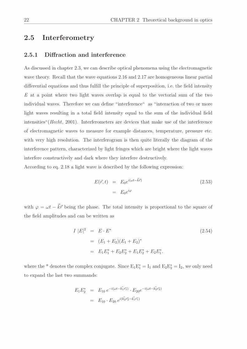
As discussed in chapter 2.3, we can describe optical phenomena using the electromagnetic
wave theory. Recall that the wave equations 2.16 and 2.17 are homogeneous linear partial
differential equations and thus fulfill the principle of superposition, i.e. the field intensity
E at a point where two light waves overlap is equal to the vectorial sum of the two
individual waves. Therefore we can define “interference“ as “interaction of two or more
light waves resulting in a total field intensity equal to the sum of the individual field
intensities“(Hecht , 2001). Interferometers are devices that make use of the interference
of electromagnetic waves to measure for example distances, temperature, pressure etc.
with very high resolution. The interferogram is then quite literally the diagram of the
interference pattern, characterized by light fringes which are bright where the light waves
interfere constructively and dark where they interfere destructively.
According to eq. 2.18 a light wave is described by the following expression:
E(~r, t) = E0ei(ωt−~k~r) (2.53)
= E0eiϕ
with ϕ = ωt − ~k~r being the phase. The total intensity is proportional to the square of
the field amplitudes and can be written as
I |E|2 = E · E∗ (2.54)
= (E1 + E2)(E1 + E2)∗
= E1E∗
1 + E2E∗
2 + E1E∗
2 + E2E∗
1 .
where the * denotes the complex conjugate. Since E1E∗
1 = I1 and E2E∗
2 = I2, we only need
to expand the last two summands:
E1E∗
2 = E10 e−i(ωt− ~k1 ~r1) · E20e−i(ωt− ~k2 ~r2)
= E10 · E20 ei( ~k2 ~r2−~k1 ~r1)

2.5 Interferometry 23
and
E2E∗
1 = E20 e−i(ωt− ~k2 ~r2) · E10e−i(ωt− ~k1 ~r1)
= E10 · E20 e−i( ~k2 ~r2−~k1 ~r1),
which yields the interference term:
E1E∗
2 + E2E∗
1 = E10 · E20
(
ei( ~k2 ~r2−~k1 ~r1) + e−i( ~k2 ~r2−
~k1 ~r1))
= 2E10 · E20 cos(~k2~r2 − ~k1~r1)
= 2√
I1I2 cos(∂) (2.55)
with ∂ = ~k2~r2 − ~k1~r1. The total field intensity is thus
I = I1 + I2 + 2√
I1I2 cos∂. (2.56)
For different points in space this total field intensity can now be, depending on I12, bigger,
smaller or equal to I1 + I2. For cos∂ = 1 the total field intensity becomes maximal:
Imax = I1 + I2 + 2√
I1I2 (2.57)
for
∂ = 0,±2π,±4π, .....
In this case the two waves interfere constructively because the phase difference is equal
to a multiple of 2π. A minimum in the total field intensity, i.e. destructive interference is
reached for
Imax = I1 + I2 − 2√
I1I2 (2.58)
when
∂ = ±π,±3π,±5π, .....
In a special case, when the amplitudes E of both waves are equal, i.e. setting I1 = I2 = I0,
eq. 2.56 can be written as
I = 2 I0 (1 + cos∂) = 4 I0 cos2∂
2. (2.59)
Fig. 2.10 illustrates the visible light fringes resulting from single slit diffraction and double
slit diffraction for a coherent light source, e.g. a helium-neon laser.

24 CHAPTER 2 Theoretical background in optics
Figure 2.10: Light fringes from a) single and b) double slit diffraction using a monochromatic
light source. From (Hecht, 2001).
Single slit diffraction
The phenomenon that plane waves are bend when interacting with obstacles is generally
called diffraction. The obstacle considered here is a narrow slit of width w. Depending on
the distance D to the obstacle one distinguishes between Fresnel diffraction (near-field) or
Fraunhofer diffraction (far-field, λ ≪ D). As the interferometric setup descibed in chapter
4 operates in the far field, only the Fraunhofer diffraction will be of interest. The intensity
distribution in the far field resulting from single slit diffraction is given by (Hecht , 2001)
I(θ) = I(0)
(
sinβ
β
)2
, (2.60)
where
β =(πw
λ
)
sin θ. (2.61)
Fig. 2.11 shows the Fraunhofer diffraction caused by a narrow slit. From eq. 2.61 it can
be seen that the intensity function has minima equal to zero when θ = ±π,±2π,±3π, ....,
i.e. sin θ = 0, so that the envelope of an interferogram, which is dominated by the intensity
distribution resulting from a single slit, is approximately given by
W =2λD
w. (2.62)
With increasing distance D from the slit the envelope function also increases, as well as
with decreasing slit width w.

2.5 Interferometry 25
Figure 2.11: Intensity distribution from Fraunhofer diffraction at a single slit. From (Hecht,
2001)
Double slit diffraction
The phenomenon of double slit diffraction is similar to the single slit diffraction, but
implementing two narrow slits of width w and distance d from each other. The inten-
sity distribution is still governed by the single slit diffraction, provided that w≪d, but
modulated with a cos2 α-function:
I(θ) = 4 I(0)
(
sin2β
β
)
cos2α (2.63)
with
α =
(
πd
λ
)
sin θ. (2.64)
Fig. 2.12 illustrates the intensity distribution for the double slit in the far field condition.
If the slit width w would be very small compared to the slit distance resulting in sin2ββ
≈1, the intensity distribution would be governed by the cos2-function given in eq. 2.59.
On the other hand, if the slit distance d decreases, the cos2-function goes to zero and
the remaining function again resembles the distribution given for the single slit. The
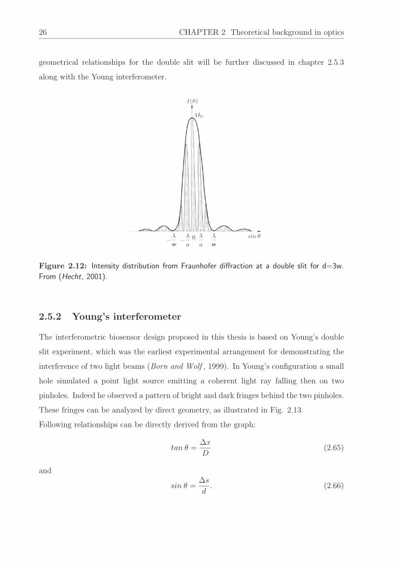
26 CHAPTER 2 Theoretical background in optics
geometrical relationships for the double slit will be further discussed in chapter 2.5.3
along with the Young interferometer.
Figure 2.12: Intensity distribution from Fraunhofer diffraction at a double slit for d=3w.
From (Hecht, 2001).
2.5.2 Young’s interferometer
The interferometric biosensor design proposed in this thesis is based on Young’s double
slit experiment, which was the earliest experimental arrangement for demonstrating the
interference of two light beams (Born and Wolf , 1999). In Young’s configuration a small
hole simulated a point light source emitting a coherent light ray falling then on two
pinholes. Indeed he observed a pattern of bright and dark fringes behind the two pinholes.
These fringes can be analyzed by direct geometry, as illustrated in Fig. 2.13.
Following relationships can be directly derived from the graph:
tan θ =∆x
D(2.65)
and
sin θ =∆s
d. (2.66)

2.5 Interferometry 27
Figure 2.13: Young’s experiment. Two slits of width w are separated by a distance d to
each other and located at distance D to a screen in the far field. ∆s denotes the difference in
path length of the two light beams.
Assuming that w≪D we can use the small-angle approximation to get
tan θ ≈ sin θ =∆x
D(2.67)
and
∆s =d∆x
D. (2.68)
Thus maxima of the intensity can be observed for
x =mDλ
d, (2.69)
when m=0,1,2.... and minima for m = 12, 3
2, 5
2, .. .
2.5.3 Influence of coherence length
So far, interference phenomena have been described provided that the light source is
monochromatic. Since the interferometric biosensor described here is mainly operated
with a partially coherent superluminescent diode (SLD), it is important to consider the
main characteristics of interference of partially coherent light. A more comprehensive and
mathematical description of the coherence properties of light can be found in (Born and
Wolf , 1999; Hecht , 2001).

28 CHAPTER 2 Theoretical background in optics
The term “coherence“describes in general the ability of two waves to combine and produce
an interference pattern. Incoherent waves are not able to produce a visible interference
pattern. Coherence can be further identified as spatial or temporal coherence (Hecht ,
2001). When a wave is coherent to itself, i.e. it is combined with a time-delayed copy
of itself, we speak of temporal coherence and define a coherence time of the wave ∆τc,
which is the duration of the delay still resulting in visible interference. From this, the
coherence length ∆xc = c∆τc is derived. This temporal coherence correlates with the
spectral bandwidth of the light source as the coherence time is inversely proportional to
the bandwidth. For example lasers, which are the most monochromatic light sources,
have very large coherence times and lengths.
Young’s experiment in fact relies on spatial coherence, which describes the ability of
any spatial position of the wave to interfere with any other spatial position. Fig. 2.14
illustrates the interference at point P of wave groups originating from point sources S1
and S2. If the difference in path length is larger than the coherence length ∆lc, the wave
group H1 for example cannot interfere with its respective wave group H2 in P due to the
relative phase difference. If now the difference in path length is smaller than the coherence
length, the wave groups can overlap and produce a stable interference pattern.
Figure 2.14: Schematic representation of double slit interference of partially coherent light
with coherence length ∆lc. a) for a path length ∆r > ∆lc b) for a path length ∆r < ∆lc.
From (Hecht, 2001).

2.5 Interferometry 29
To describe the coherence mathematically, we define a so-called complex degree of coher-
ence γ12(τ) and insert it into eq. 2.56 (Born and Wolf , 1999):
I = I1 + I2 + 2√
I1I2 γ12(τ) cos∂ (2.70)
We now consider quasi-monochromatic light where the spectral bandwidth ∆ν is suffi-
ciently small. Provided that the intensities are equal, i.e. I1 = I2, the visibility of the
fringes is then equal to the degree of coherence. As illustrated in Fig. 2.14, for the case
of coherent light, the visibility is fully modulated with 4I, for partially coherent light
the visibility becomes less modulated with 2I, and for an incoherent superposition the
visibility equals zero. Transferred to an interferogram pattern as observed in the Young
Figure 2.15: Intensity distribution in the interferogram produced by a quasi-monochromatic
light source. For equal intensities I1 and I2 and a degree of coherence γ12 a) coherent
superposition with γ12 = 1 b) partially coherent superposition with 0 < γ12 < 1 c) incoherent
superposition with γ = 0. From (Born and Wolf , 1999).
configuration, we obtain an interferogram with high visibility for a coherent light source
with a narrow bandwidth, and a less modulated interferogram for a partially coherent
light source with a broader bandwidth, as shown in Fig. 2.15. Both interferograms can be
obtained with the Young interferometric setup described in chapter 4, but with different
spectral filtering methods. Especially for signal analysis purposes it is important that both
signatures can be evaluated with different algorithms. Flowcharts of these algorithms are
presented in Appendix D.

30 CHAPTER 2 Theoretical background in optics
b)a)
inte
nsity
[a.u
.]
pixel
inte
nsity
[a.u
.]
pixel
Figure 2.16: a) Far-field interference pattern of a coherent light source, simulated. The
interferogram is characterized by a high degree of coherence and thus a high visibility (≈ 1).
b) Far-field interference pattern of a partially coherent light source, simulated. The region of
interference is narrower than in a).
2.6 Fourier transform analysis for signal processing
The interferometric biosensor is designed to obtain phase information from a periodic
signal, the interferogram. The question is how to process this phase information with
appropriate and efficient mathematical algorithms to determine a change in signal. Signal
analysis provides many different transform algorithms suited for such applications. Since
the interferograms obtained from the interferometric biosensor are periodic signals, the
main approach evaluating these signals is the Fourier transform and shall be presented
briefly in this chapter.
A profound description of Fourier transform analysis is clearly beyond the scope of this
thesis and is described elsewhere (Lang and Pucker , 1998; Meyer , 2003; Schrufer , 1992).
Fourier series
The Fourier Transform (FT) has been developed in the beginning of the 19th century by
Joseph Fourier based on the discovery that any periodic signal consists of single sine and
cosine waves that can be used to reproduce the signal:
ak =2
T
∫ T
0
x(t) cos(kω0t) dt (2.71)

2.6 Fourier transform analysis for signal processing 31
bk =2
T
∫ T
0
x(t) sin(kω0t) dt, (2.72)
with T = 1f0
being the period of the function. Without the proof given here these two
functions can be represented by the Fourier series given by
x(t) =a0
2+
∞∑
k=1
(ak cos(kω0t) + bk cos(kω0t)) . (2.73)
With Euler’s identity
eikω0t = cos(kω0t) + sin(ikω0t) (2.74)
we get the Fourier series in complex form:
x(t) =∞
∑
k=1
cn eikω0t. (2.75)
By multiplication of eq. 2.75 with e−ikω0t and integration we obtain the complex Fourier
coefficients:
cn =1
T
∫ T
0
x(t) e−ikω0t dt (2.76)
for integration over exactly one period T. A problem arises when applying the FT on
aperiodic signals, because then the period approaches infinity and thus the fundamental
frequency approaches zero. With this limit, as f0 → 0, the sum in the Fourier series can
be replaced by an integral. The new function in frequency is represented X(ω), and the
Fourier transform of this function can be written as
x(t) =1
2π
∫
∞
−∞
X(ω) eiωt dω. (2.77)
From the Fourier transform of a function of time the original function of time can always
be recovered, i.e. either x(t) or X(ω) describe a function uniquely, which is also stated by
the Inverse Fourier transform given by
X(ω) =
∫
∞
−∞
x(t) e−iωt dt. (2.78)
These two equations are the fundamentals for the interferogram signal evaluation, where
a position-dependent periodic function is detected and analyzed by a FT in the spatial
frequency domain to obtain the period of the interferogram and thus the information
about changes in the phase velocity of the two optical beams.

32 CHAPTER 2 Theoretical background in optics
Discrete signals and Discrete Fourier Transform
The considerations above are clearly valid for continuous signals, i.e. along an axis a data
value exists for any infinitesimal interval on this axis. In digital signal analysis, however,
mostly discrete signals have to be dealt with. Discrete signals are simply signals that
are not continuous in time or space. For example a CCD camera would detect a data
value for each single pixel. In this case the signal is described as discrete along the spatial
axis. The question is if discrete signals provide the same information than continuous
signals, and if there is a minimum of signal values needed to obtain useful information.
Nyquist’s Theorem (Meyer , 2003) states that a continuous signal with frequency fc can
be reconstructed without error from its sampled version with frequency fs if
fs ≥ 2 fc. (2.79)
In words, the sampling frequency for the discrete signals must be greater than twice the
maximum frequency of the signal being sampled.
Transferred to the interferometric biosensor this means that, the CCD detector regarded
as a spatial axis, each pixel corresponds to a single detector having a certain intensity
value. Nyquist’s Theorem is fulfilled as long as the period of the detected interferogram
is greater than 2 pixels.
Fast Fourier Transform
As described above, in most cases data points are sampled in a discrete, equidistant
form and not as a continuous function. Consequently the Fourier integrals have to be
modified, i.e. the Fourier sum in exponential form and the calculation of the coefficients
(2.75 and 2.76) have to be converted into a discrete form with a finite number of data
points (Discrete Fourier Transform, DFT). In numerical applications the integrals over
functions are approximated by weighted sums over the data points at so-called nodes.
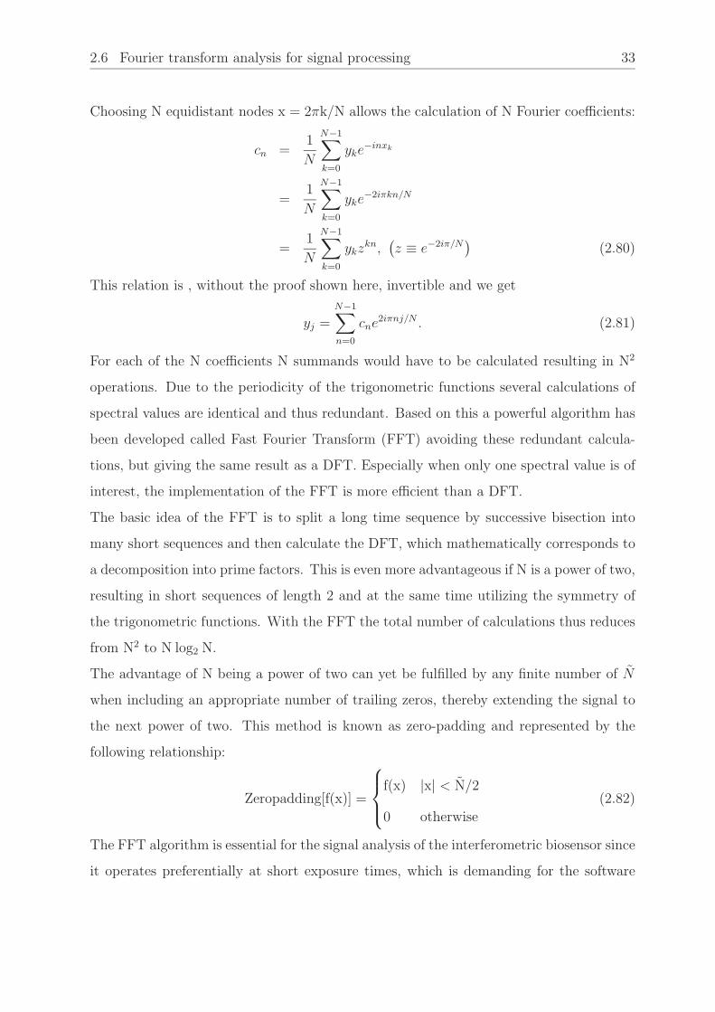
2.6 Fourier transform analysis for signal processing 33
Choosing N equidistant nodes x = 2πk/N allows the calculation of N Fourier coefficients:
cn =1
N
N−1∑
k=0
yke−inxk
=1
N
N−1∑
k=0
yke−2iπkn/N
=1
N
N−1∑
k=0
ykzkn,
(
z ≡ e−2iπ/N)
(2.80)
This relation is , without the proof shown here, invertible and we get
yj =N−1∑
n=0
cne2iπnj/N . (2.81)
For each of the N coefficients N summands would have to be calculated resulting in N2
operations. Due to the periodicity of the trigonometric functions several calculations of
spectral values are identical and thus redundant. Based on this a powerful algorithm has
been developed called Fast Fourier Transform (FFT) avoiding these redundant calcula-
tions, but giving the same result as a DFT. Especially when only one spectral value is of
interest, the implementation of the FFT is more efficient than a DFT.
The basic idea of the FFT is to split a long time sequence by successive bisection into
many short sequences and then calculate the DFT, which mathematically corresponds to
a decomposition into prime factors. This is even more advantageous if N is a power of two,
resulting in short sequences of length 2 and at the same time utilizing the symmetry of
the trigonometric functions. With the FFT the total number of calculations thus reduces
from N2 to N log2 N.
The advantage of N being a power of two can yet be fulfilled by any finite number of N
when including an appropriate number of trailing zeros, thereby extending the signal to
the next power of two. This method is known as zero-padding and represented by the
following relationship:
Zeropadding[f(x)] =
f(x) |x| < N/2
0 otherwise
(2.82)
The FFT algorithm is essential for the signal analysis of the interferometric biosensor since
it operates preferentially at short exposure times, which is demanding for the software

34 CHAPTER 2 Theoretical background in optics
and fast processing is needed. Therefore a FFT algorithm using zero-padding has been
implemented into the signal analysis software as described in Appendix D and chapter
4.2.4.
2.7 Signal analysis and processing
2.7.1 System principles and relationships
For signal processing and evaluation the basic system principles and relationships have
to be known. These relationships have already been described in Brandenburg (1997);
MacKenzie (2003) and shall be summarized here.
Recall the intensity distribution from Young’s double slit experiment (eq. 2.59):
I(x) ∝ cos2(φ(x) − δ), (2.83)
where φ(x) = 2πx/p with p being the spatial period of the cos2-function and x the off-
set along the detection axis. δ denotes an additional phase shift. The period of the
interferogram is given by
p =Dλ
d. (2.84)
Inserting eq. 2.84 into eq. 2.83 yields
∆φ =2πd∆x
Dλ(2.85)
=2π∆s
λ.
The phase shift is a measure for a change in phase velocity, and thus a change in the
effective refractive index, on one of both channels. According to (Brandenburg , 1997),
this phase shift is given by the following relationship:
∆φ =2πL∆neff
λ, (2.86)
with L being the interaction length. For the spatial offset follows:
∆x =DL∆neff
d. (2.87)
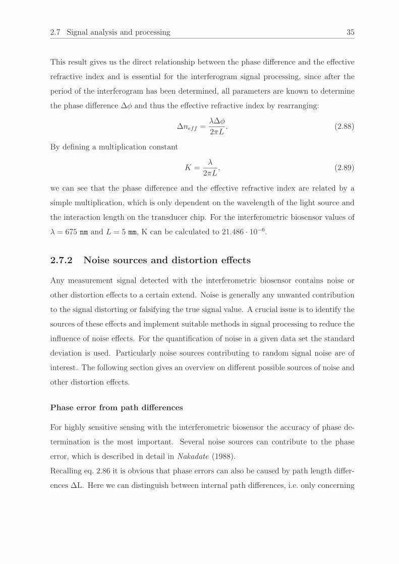
2.7 Signal analysis and processing 35
This result gives us the direct relationship between the phase difference and the effective
refractive index and is essential for the interferogram signal processing, since after the
period of the interferogram has been determined, all parameters are known to determine
the phase difference ∆φ and thus the effective refractive index by rearranging:
∆neff =λ∆φ
2πL. (2.88)
By defining a multiplication constant
K =λ
2πL, (2.89)
we can see that the phase difference and the effective refractive index are related by a
simple multiplication, which is only dependent on the wavelength of the light source and
the interaction length on the transducer chip. For the interferometric biosensor values of
λ = 675 nm and L = 5 mm, K can be calculated to 21.486 · 10−6.
2.7.2 Noise sources and distortion effects
Any measurement signal detected with the interferometric biosensor contains noise or
other distortion effects to a certain extend. Noise is generally any unwanted contribution
to the signal distorting or falsifying the true signal value. A crucial issue is to identify the
sources of these effects and implement suitable methods in signal processing to reduce the
influence of noise effects. For the quantification of noise in a given data set the standard
deviation is used. Particularly noise sources contributing to random signal noise are of
interest. The following section gives an overview on different possible sources of noise and
other distortion effects.
Phase error from path differences
For highly sensitive sensing with the interferometric biosensor the accuracy of phase de-
termination is the most important. Several noise sources can contribute to the phase
error, which is described in detail in Nakadate (1988).
Recalling eq. 2.86 it is obvious that phase errors can also be caused by path length differ-
ences ∆L. Here we can distinguish between internal path differences, i.e. only concerning
36 CHAPTER 2 Theoretical background in optics
the sensing area on the transducer chip, and external path differences, i.e. path differences
in the system mainly caused by misalignment or displacements of optical components.
An internal path difference ∆L = L2 − L1 is limited by differences in the interaction
lengths L1 and L2 on the transducer chip, i.e. between the two gratings. However, even
if L1 differs from L2 due to fabrication defects in the gratings, this path difference would
be static and not contributing to phase noise. Internal path differences can thus only be
influenced by wavelength fluctuations of the light source, which will be discussed below.
External path differences can occur anywhere in the optical beam path e.g. by misaligned
optical components. Yet this path difference would also be of a static nature and not
cause noise or fluctuations in the measurement signal. Here the limiting factors would
be external vibrations or again wavelength instabilities leading to fluctuating path dif-
ferences. A continuous temperature change, i.e. wavelength instability, would therefore
cause a drift in the interferogram signal.
Noise from light source instability
Since the interferometric biosensor is mostly operated with an SLD, the instability of this
light source is the most important. When recalling eq. 2.86, we can see that a fluctuation in
wavelength would directly lead to a phase change and therefore in ∆neff . The uncertainty
in wavelength of the SLD can, as described in more detail in the experimental section, be
estimated to be ≈ 10−3nm. This results in a contribution to the total signal noise in the
order of ≈ 10−9 in ∆neff .
Mechanical noise sources
Mechanical noise sources can mainly arise from disturbances in the hardware components
of the system, e.g. component construction defects or misalignment of the components
resulting in a path length difference. Another source for mechanical noise are physical
vibrations in the system also causing path length differences contributing to phase noise.

2.7 Signal analysis and processing 37
Electronic noise sources
In electronical systems there exist various types of electronic noise sources, among them
thermal noise, shot noise and readout noise which shall be described here briefly (Lindner
et al., 1999):
• Thermal noise: in a CCD camera, single electrons in the sensor chip may have
enough energy from random thermal motion to overcome the difference of potential
and accumulate with the photoelectrons, contributing to the total photocurrent.
This additional current is called dark current, which is linearly dependent on the
exposure time of the camera. Since it also depends on the ambient temperature, it
is feasible to cool the camera for long exposure times (> 1s). Thermal noise is white
noise, i.e. the frequency amplitudes are characterized by a Gaussian distribution.
• Shot noise (quantum noise): shot noise is caused by frequent fluctuations of the
current in a conducting material resulting from diffusion of charge carriers and the
random generation or recombination of electron-hole pairs. Shot noise is also white
noise.
• Readout noise: contains noise caused by transfer noise (readout of photoelectrons in
the CCD sensor), noise caused by analog-digital conversion and noise in the signal
amplifier. Readout noise is characteristic for the type of camera, independent on
exposure time, and contributes to a large extend to the total noise in a system.
The total noise is calculated from contributions from dark current and noise in the signal:
σtot =√
σ2signal + σ2
DC (2.90)
For short exposure times the noise caused by dark current can be neglected.
Quantization noise and aliasing
These two sources of noise are associated with the FFT and its obtained accuracy. Quan-
tization noise arises from quantization processes, i.e. the conversion from an analog into
its digital approximation, in our case in the CCD camera and its electronics. As stated

38 CHAPTER 2 Theoretical background in optics
by Kujawinska and Wojciak (1991), quantization noise can be neglected when converting
the signals with more than 6bit. As the CCD sensor used for the interferometric biosensor
operates with either 12bit or 16bit conversion, phase errors resulting from quantization are
negligible. Aliasing is an effect occuring when the Nyquist Theorem (2.6) is not fulfilled,
i.e. the chosen sampling frequency is too low. In this case the signal frequency is overlaid
by a higher frequency distorting the reconstructed signal. As mentioned in chapter 1.6,
aliasing occurs in our case only if the interferogram period was less than two pixels on
the CCD camera.
2.7.3 Signal filtering methods
In data sampling the standard deviation of a data distribution is considered to be a
measure for variation in the signal. Since the standard deviation is higher in noisier
data, it is an important task of signal processing to apply filtering methods to reduce the
noise in data distributions, here in phase noise. An efficient way of reducing phase noise
is the application of averaging filters, or sometimes window functions. Two averaging
filters shall be introduced here briefly considering their use for the interferometer signal
processing software.
Implementation of window functions
One method in digital filtering is to apply a window function to the detected data set
for a more precise extraction of information. Typical window functions for interferogram
distributions shown in chapter 2.5.2 would be the von Hann-window or Hamming window
function. These two common functions have already been tested for their suitability for
noise reduction in the interferometric biosensor by MacKenzie (2003). It was shown that
the implementation of window functions within the signal processing algorithm used for
the interferometric biosensor has no significant effect on noise reduction.
2.7 Signal analysis and processing 39
Block average filter
The block average filter, as the name implies, calculates the average of a block of n data
points by adding all n data values and subsequently dividing by an averaging factor N.
Fig. 2.17 illustrates the flow chart of a block average filter.
Figure 2.17: Flow chart of a block average filter for averaging a data series of size n.
Adapted from (MacKenzie, 2003)
Applying this filter means a reduction of N input data points to n=n/N. This filter is
useful when a reduction of the number of data points is desired, e.g. to save memory due
to a smaller data file. However, the filter is quite calculation intensive and can only be
applied after the complete sequence of n data points has been recorded.
Moving average filter
To improve the calculation efficiency, a so-called recursive filter may be applied that only
depends on the previously calculated value and the most recently sampled data value.
Fig. 2.18 illustrates this graphically.
This filter is known as moving average filter because a moving window of the most recent
n data points is used to calculate the average. In other words, the oldest data value in
the buffer is continuously replaced by the newly measured one, maintaining a constant
number of n data values in the buffer. Thus the total number of averaged values for a given
time is the same as without averaging. Furthermore, the buffer is filled only once at the
beginning of the filtering process unlike the block average where the buffer is consistently
filled and emptied. This method of filtering has the feature of weighting all data points

40 CHAPTER 2 Theoretical background in optics
Figure 2.18: Flow chart of a moving average filter for averaging a data series of size n.
Adapted from (MacKenzie, 2003)
equally, i.e. a given data point in the past within the buffer has the same influence on the
averaged value than a more recent one. However, this equal weighting of all data points
by the moving average is only feasible when the mean value of all data points remains
approximately constant (baseline). As soon as the data curve follows a certain trend, in
our case e.g. a binding event, care has to be taken to not choose the buffer size n too large
as then the averaged data might distort the real data.

Chapter 3
Theoretical background in
biochemistry
3.1 Introduction
The core of any label-free biosensor is represented by the transducer with its actual sen-
sor surface, since it acts as a functional linker between the biochemical reaction and the
transducer. Ideally a sensor surface should be prepared in such a way that a variety
of immunoassays can be performed. In this chapter a brief overview of immunoassay
design, surface chemistry and preparation, and binding reaction kinetics will be given.
Detailed experiments on the characterization of the linking chemistry for the interfero-
metric biosensor will be described in chapter 5 along with the application measurements.
3.2 Immunoassays
Since the late 1960’s, immunoassays have proven to be very powerful tools in life science,
pharmaceutical and medical research for the elucidation of biochemical processes (Davies ,
2001). Immunoassays use antibodies to detect, usually labeled, analyte molecules, e.g. anti-
gens, with high specificity and strong binding characteristics. A typical assay comprises at
41

42 CHAPTER 3 Theoretical background in biochemistry
Figure 3.1: One-step immunoassay. 1. Buffer is run over a surface with immobilized
antibodies (baseline). 2. The analyte solution with antigen is added, antigen binds to the
antibodies until an equilibrium of free/bound antigen is reached. 3. Buffer is run again over
the surface so that unbound antigen is washed away.
Figure 3.2: Multi-step immunoassay. 1. Buffer is run over a surface with immobilized
antibodies (baseline). 2. The analyte solution with antigen is added, antigen binds to the
antibodies until an equilibrium of free/bound antigen is reached. 3. Buffer is run again over
the surface so that unbound antigen is washed away. 4. Analyte solution with a secondary
antibody is added, antibody binds to the antigen until equilibrium is reached. 5. Buffer wash
to remove unbound antibody.

3.3 Surface chemistry 43
least one immobilized capture molecule, i.e. bound to a solid phase, in our case the wave-
guide surface, and an analyte in solution which is captured by the immobilized molecules.
The simplest immunoassay is the so-called immunometric one-step assay, where an anti-
body is immobilized on the sensor surface, and its corresponding antigen is bound from
the liquid phase. Multistep assays would work with a labeled secondary antibody binding
to the antigen, giving the detection signal, as it is the case for the so-called sandwich
assay. A comprehensive description of different types of immunoassays including labeled
reagents can be found in Davies (2001).
Label-free immunoassays usually work as one-step assay with an immobilized capture
molecule and its corresponding analyte in solution, as the signal depends on a change
in surface mass coverage and a label for signal detection is not needed. This saves both
reagents for labeling such as fluorescent dyes and time for realization of the assay.
3.3 Surface chemistry
For the realization of a stable and reproducible immunoassay, the molecules of interest
have to be linked to the waveguide surface in an appropriate way. The Ta2O5 surface is
relatively hydrophilic by nature, so that most proteins or antibodies, when brought on the
surface, would merely stick to the surface in a random orientation and could be washed
away quite easily. For this reason a stable, bifunctional linking molecule is desirable, which
can be covalently bound to the Ta2O5 surface with one end and at the same time pro-
vide a functional group for the oriented immobilization of biomolecules on the other end.
Depending on the waveguide substrate, there exists a wide variety of linking chemistries,
e.g. reagents forming self-assemled monolayers (SAM), among them modified alkyl thiols
or modified silanes. For Ta2O5 , mostly the use of silanes has been described in literature
(Polzius et al., 1996; Laureyn et al., 2001). For the interferometric biosensor, two dif-
ferent silanes have been tested and characterized, 3-Aminopropyl-triethoxysilane (APTS)
and 3-Glycidoxy-propyl-triethoxysilane (GOPS). Both silanes are trifunctional, i.e. pro-
vide three hydrolyzable functional head groups, and are able to form a two-dimensional
network on the waveguide surface (Tovar , 1995). Due to these crosslinks, a trifunctional

44 CHAPTER 3 Theoretical background in biochemistry
Figure 3.3: Chemical formulas for 3-Glycidoxypropyl-triethoxysilane (left) and 3-
Aminopropyl-triethoxysilane (right). The silane is covalently coupled to the waveguide surface
via hydroxyl groups, the functional group for biomolecule binding is an epoxy-group for GOPS
and an amino-group for APTS.
silane yields a greater stability than mono- or bifunctional silanes.
APTS provides an amino-group as functional linker for the covalent coupling of biomolecules,
GOPS an epoxy-group. Depending on the assay and the proteins/antibodies involved,
these functional groups can be further modified for a stable immobilization. For example,
biotin with a special linker can be attached to the amino-modified surface to bind strep-
tavidin (see chapter 3.5). This streptavidin surface is a commonly used basis for assays
with biotinylated reagents (Morgan and Taylor , 1992; Busse et al., 2002).
The kind of capture molecule immobilization always depends on the kind of assay and
purpose of study. For kinetics and affinity measurements, preferably a rather low receptor
density which is still giving a good signal should be used to avoid any secondary effects
such as mass transport limitations or steric hindrances. In this case immobilization can
be done by mere adsorption of the receptor to the waveguide. The kind of immobiliza-
tion should also be taken into consideration when choosing the appropriate regeneration

3.4 Kinetics of binding reactions 45
buffer.
In contrast, for concentration measurements the receptor density needs to be as high
as possible to detect even smallest concentrations of the ligand. Here, silanization of
the waveguide surface for oriented coupling of the receptor is advisable to reach a high
receptor density. The same is valid for studies with molecules of low molecular weight.
3.4 Kinetics of binding reactions
With the interferometric biosensor it is feasible to monitor binding reactions time-resolved
and thus information about kinetics of the reaction is accessible. Binding kinetics play
a crucial role in the successful development of an immunoassay and new methods of
assay optimization are developed constantly. Each immunoassay consists of at least one
binding reaction, usually between an antibody and its antigen. Here a brief theoretical
description about binding kinetics for a pseudo-first order reaction shall be given. More
detailed considerations can be found in Davies (2001).
3.4.1 The 1:1 interaction model
A biochemical interaction like the antibody-antigen reaction can simplistically be de-
scribed by the Law of Mass Action (Karlsson and Lofas , 1998):
cAg + cAbka,kd↔ cAb−Ag (3.1)
wherecAg = concentration of antigen [M]
cAb = concentration of antibody [M]
cAb−Ag = antibody-antigen complex [M]
ka = association rate constant [M−1 · s−1]
kd = dissociation rate constant [s−1].
This model implies a 1:1 binding reaction, i.e. one immobilized molecule captures exactly
one analyte molecule (monovalent) from the solution. Further it is assumed that the
detected signal ∆neff is directly proportional to the change in surface mass coverage.
Also, there should be no unspecific binding caused by any other substances in the analyte

46 CHAPTER 3 Theoretical background in biochemistry
solution which could possibly contribute to the signal and thereby giving a false positive.
This can be avoided by assay optimization and will be further discussed in chapter 6.
Taking all this into account, we can describe the time-dependence of the binding reaction
as follows:
∂cAb−Ag
∂t= ka · cAg · cAb − kd · cAb−Ag (3.2)
= ka · cAg · cAbt− ka · cAg · cAb−Ag − kd · cAb−Ag
= ka · cAg · cAbt− cAb−Ag · (ka · cAg + kd),
with
cAbt= cAb−Ag + cAb being the total concentration of antibody.
Assuming
cAb−Ag(t = 0) = 0 (boundary condition),
it can be easily proven that
cAb−Ag(t) =ka · cAg · cAbt
ka · cAg + kd
· (1 − e−(ka·cAg+kd)·t) (3.3)
is a solution of this differential equation giving the time-dependence of the binding reac-
tion. For t → ∞, i.e. when reaching equilibrium, this can be expressed by
cAb−Agequil.=
ka · cAg · cAbt
ka · cAg + kd
, (3.4)
which is also known as the Langmuir isotherm for a one-site binding model. Introducing
the affinity constant of the system
K =ka
kd
[M−1], (3.5)
we get
cAb−Agequil.=
cAg · cAbt
1K
+ cAg
. (3.6)

3.4 Kinetics of binding reactions 47
On the other hand, for small t, i.e. t ≪ 1kd+ka·cAg
, eq. (3.3) can be expanded in a Taylor
series:
cAb−Ag(t) =ka · cAg · cAbt
ka · cAg + kd
[(kd + ka · cAg) · t + O2(t)], (3.7)
where the linear approximation shows that
∂cAb−Ag
∂t≈ ka · cAbt
· cAg. (3.8)
Equation (3.8) implies that the initial binding rate∂cAb−Ag
∂tis linear in cAg. Thus it is
possible to determine the binding rate constants ka, kd and the affinity constant K from a
time-resolved measurement curve comprising several, at least five, different concentrations
of the analyte: a plot of the end signal values of each concentration versus the concentra-
tion itself (dose-response curve) can be fitted to the Langmuir isotherm given in eq. 3.6,
yielding the maximum antigen concentration (which equals cAbt, since in this case each
antibody has bound one antigen and a so-called antigen monolayer has been formed) and
the affinity constant K.
Figure 3.4: Dose-response curve. The end signal values are plotted versus the respective
concentration and fitted to the Langmuir isotherm described in eq. 3.6 to obtain the maximum
antigen concentration (monolayer) signal and the affinity constant K of the system. Adapted
from Davies (2001).
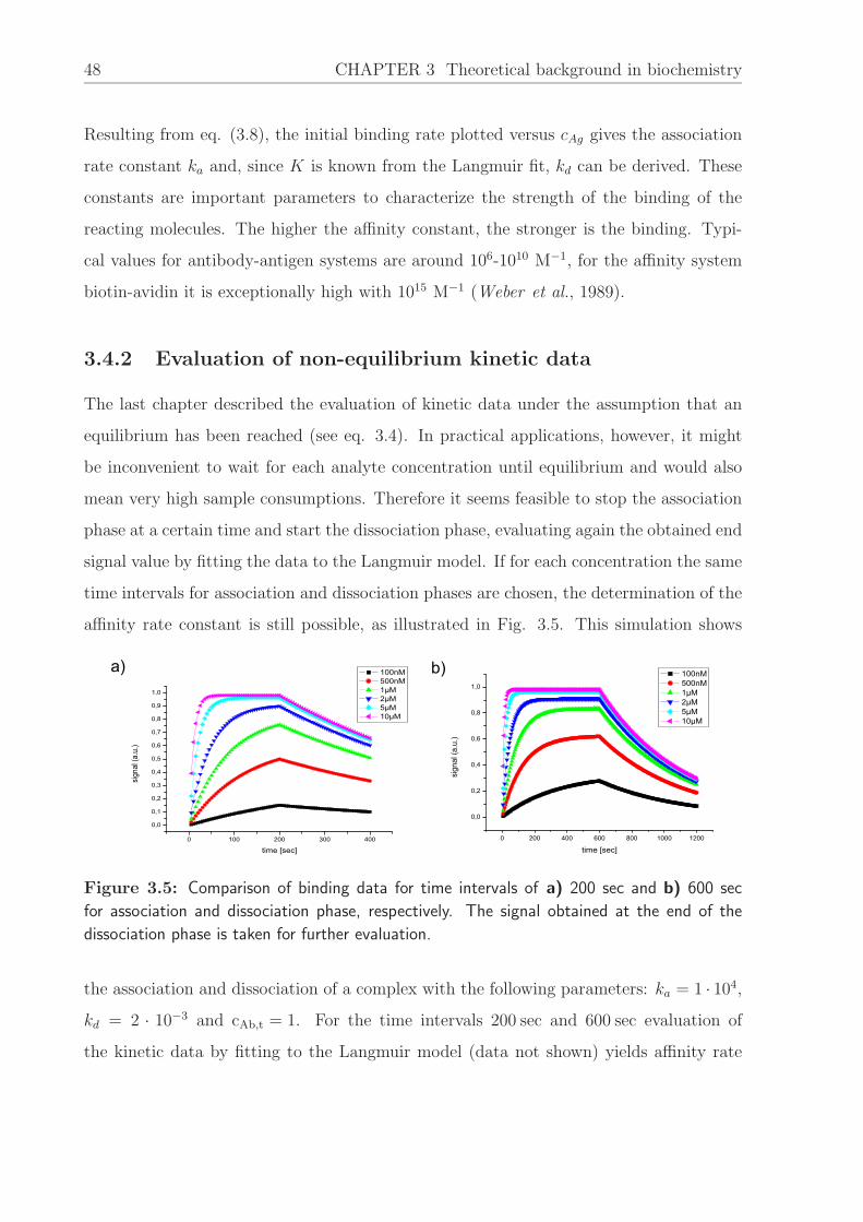
48 CHAPTER 3 Theoretical background in biochemistry
Resulting from eq. (3.8), the initial binding rate plotted versus cAg gives the association
rate constant ka and, since K is known from the Langmuir fit, kd can be derived. These
constants are important parameters to characterize the strength of the binding of the
reacting molecules. The higher the affinity constant, the stronger is the binding. Typi-
cal values for antibody-antigen systems are around 106-1010 M−1, for the affinity system
biotin-avidin it is exceptionally high with 1015 M−1 (Weber et al., 1989).
3.4.2 Evaluation of non-equilibrium kinetic data
The last chapter described the evaluation of kinetic data under the assumption that an
equilibrium has been reached (see eq. 3.4). In practical applications, however, it might
be inconvenient to wait for each analyte concentration until equilibrium and would also
mean very high sample consumptions. Therefore it seems feasible to stop the association
phase at a certain time and start the dissociation phase, evaluating again the obtained end
signal value by fitting the data to the Langmuir model. If for each concentration the same
time intervals for association and dissociation phases are chosen, the determination of the
affinity rate constant is still possible, as illustrated in Fig. 3.5. This simulation shows
b)a)
0 100 200 300 400
0,0
0,1
0,2
0,3
0,4
0,5
0,6
0,7
0,8
0,9
1,0
100nM 500nM 1µM 2µM 5µM 10µM
signa
l (a.u.)
time [sec]
0 200 400 600 800 1000 1200
0,0
0,2
0,4
0,6
0,8
1,0
100nM 500nM 1µM 2µM 5µM 10µM
sign
al (a
.u.)
time [sec]
Figure 3.5: Comparison of binding data for time intervals of a) 200 sec and b) 600 sec
for association and dissociation phase, respectively. The signal obtained at the end of the
dissociation phase is taken for further evaluation.
the association and dissociation of a complex with the following parameters: ka = 1 · 104,
kd = 2 · 10−3 and cAb,t = 1. For the time intervals 200 sec and 600 sec evaluation of
the kinetic data by fitting to the Langmuir model (data not shown) yields affinity rate
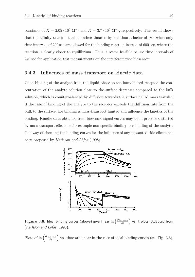
3.4 Kinetics of binding reactions 49
constants of K = 2.05 · 106 M−1 and K = 3.7 · 106 M−1, respectively. This result shows
that the affinity rate constant is underestimated by less than a factor of two when only
time intervals of 200 sec are allowed for the binding reaction instead of 600 sec, where the
reaction is clearly closer to equilibrium. Thus it seems feasible to use time intervals of
240 sec for application test measurements on the interferometric biosensor.
3.4.3 Influences of mass transport on kinetic data
Upon binding of the analyte from the liquid phase to the immobilized receptor the con-
centration of the analyte solution close to the surface decreases compared to the bulk
solution, which is counterbalanced by diffusion towards the surface called mass transfer.
If the rate of binding of the analyte to the receptor exceeds the diffusion rate from the
bulk to the surface, the binding is mass-transport limited and influence the kinetics of the
binding. Kinetic data obtained from biosensor signal curves may be in practice distorted
by mass-transport effects or for example non-specific binding or rebinding of the analyte.
One way of checking the binding curves for the influence of any unwanted side effects has
been proposed by Karlsson and Lofas (1998).
Figure 3.6: Ideal binding curves (above) give linear ln(
∂cAb−Ag
∂t
)
vs. t plots. Adapted from
(Karlsson and Lofas, 1998).
Plots of ln(
∂cAb−Ag
∂t
)
vs. time are linear in the case of ideal binding curves (see Fig. 3.6),
50 CHAPTER 3 Theoretical background in biochemistry
and deviate from this linearity when the measurement data is distorted by mass transport
or other side effects. In practice lower receptor capacities or higher flow rates ensure that
mass-transport limitations do not occur (Myszka, 1999). Another mathematical model
(Myszka et al., 1998) describes how to interpret mass transport-influenced data in cases
when mass transport limitating assay conditions cannot be avoided. Furthermore it is nec-
essary to check for rebinding, i.e. analyte molecules rebind to another receptor molecule
during the dissociation phase leading to a falsified dissociation curve. It has been shown
that rebinding is a crucial issue when small molecules are involved and binding rate con-
stants derived from biosensor binding curves may vary significantly from rate constants
obtained by measurements in solution (Nieba et al., 1996).
3.5 Biochemical background on the application mea-
surement reagents
The quality of a biosensor response clearly depends on the quality and specificity of the
biochemical reagents. A subclass of biosensors are called immunosensors, i.e. immobilized
antibodies or antigens are used as receptors for their respective immunoreaction ligand.
Two affinity systems used in our experiments will be introduced briefly concerning their
biochemical background, the immunoreaction system immunoglobulin G-protein G (or
protein A) and the affinity system biotin-streptavidin, which is the basis for measurements
with biotinylated reagents. Further information about the biochemical backgrounds be-
yond the scope of this thesis can be found in (Lehninger et al., 1994; Lottspeich and
Zorbas , 1998).
3.5.1 Immunoreactands Immunoglobulin G - Protein G or A
Antibodies are glycoproteins belonging to the immunoglobulin family comprising many
proteins involved in immune recognition and host defense systems (Davies , 2001). Im-
munoglobulins (Ig’s) are divided into five subclasses - IgG, IgM, IgA, IgD and IgE, differing
in size, charge, amino acid composition and carbohydrate content. Here the IgG shall be

3.5 Biochemical background on the application measurement reagents 51
described briefly as it is relevant for the experiments shown in chapter 5.
The basic structure of an IgG looks Y-shaped and consists of four different polypeptide
chains (see Fig. 3.7) with a total molecular weight of 156kDa : two larger ones (designated
as “H“ for heavy) and two smaller chains (with “L“ for light). All these chains (primary
structures) are mixes of α-helices and β-pleated sheets (secondary structures). The four
chains are linked by disulfide bonds as indicated by the dots to create an overall tertiary
structure. Both H and L chains end in a highly individualized portion (blue), and these
pairs are specific for a type of antigen. Therefore each IgG is bivalent, i.e. able to bind
two antigens of the same type. Regions of antigens recognized and bound by the antibody
are called epitopes. As each IgG out of millions of different IgG’s has different blue ends,
these ends are called variable (“V“). In contrast, the parts shown in white are uniformly
structured among the IgG molecules and are therefore called constant (“C“) regions. In
fact, by the constant regions the different Ig subclasses can be distinguished.
Figure 3.7: Schematic structure of an IgG antibody. The molecule (M=156 kDa) consists
of four polypeptide chains, two heavy chains (“H“) and two light chains (“L“). The four
chains are linked by disulfide bonds. The constant part common to all IgG’s is denoted with
“C“(white), the variable part different for each IgG in blue with “V“.
IgG is used almost exclusively in immunoassays due to its high yield in the immunization
process, high binding affinity to its epitope and comparably high stability during purifi-
cation and isolation (Davies , 2001). Furthermore it possesses several functional sites for
antigen binding and can easily be fractionated into its Fab and Fc fragments, resulting in
a higher specificity for particular assays. Two different IgG-binding proteins have been

52 CHAPTER 3 Theoretical background in biochemistry
used in our experiments, protein G and protein A, and their kinetic interaction evaluated
(see chapter 5).
Figure 3.8: Stick model of a human immunoglobulin G antibody created with RasMol
software (Sayle, 1993). Different colors represent the four polypeptide chains: the two heavy
chains dark and bright blue, the two light chains in yellow and green and the carbohydrate
attached to the heavy chains in red. The rotational symmetry about a vertical axis can be
clearly recognized.
Protein G is a bacterial cell wall protein with affinity for IgG, isolated from the cell walls
of group G Streptococcus sp. It has a molecular weight of approx. 33.8 kDa and is capable
of binding two IgG Fc-sites (Bjorck and Kronwall , 1984).
Protein A is a surface protein of Staphylococcus aureus with a molecular weight of ap-
prox. 41 kDa (Surolia et al., 1982) and also binds the Fc-fragment of IgG. Protein G has
a higher affinity to IgG than protein A.
3.5.2 Affinity system biotin - streptavidin
As mentioned above, the biotin-streptavidin complex is of special interest for immobi-
lization purposes because this complex has the largest free energies of association yet

3.5 Biochemical background on the application measurement reagents 53
observed for noncovalent binding of a protein and a small ligand. The complex is also
very stable over a wide range of temperature and pH and unaffected by many organic
solvents and other denaturing agents (Savage, 1992). Avidin, which is closely related to
streptavidin, is a protein originally isolated from chicken egg white and consists of four
subunits. Streptavidin is a tetrameric, biotin-binding protein isolated from the bacterium
Streptomyces avidinii. It also consists of four subunits, i.e. it binds four moles of biotin
per mole protein, with a subunit molecular weight of 16.5 kDa. Although avidin and
streptavidin show an equally high affinity to biotin, they are different in molecular weight
and isoelectric point and differ greatly in overall amino acid composition. Streptavidin
exhibits reportedly less non-specific binding than avidin (Lane, 1998), which is the main
reason for using streptavidin in our experiments. Fig. 3.9 shows a stick model of strepta-
vidin with biotin.
Figure 3.9: Stick model of a streptavidin-biotin complex created with RasMol software
(Sayle, 1993). The different blue shades represent the four subunits, the biotin molecule is
shown in green.
Biotin is the naturally occuring vitamin H found in every living cell with a molecular
mass of only 244.31 Da. The biotin molecule used in our experiments is modified with
an N-Hydroxysuccinimide (NHS)-ester and a long-chain (LC) spacer arm of 22 A. Ad-
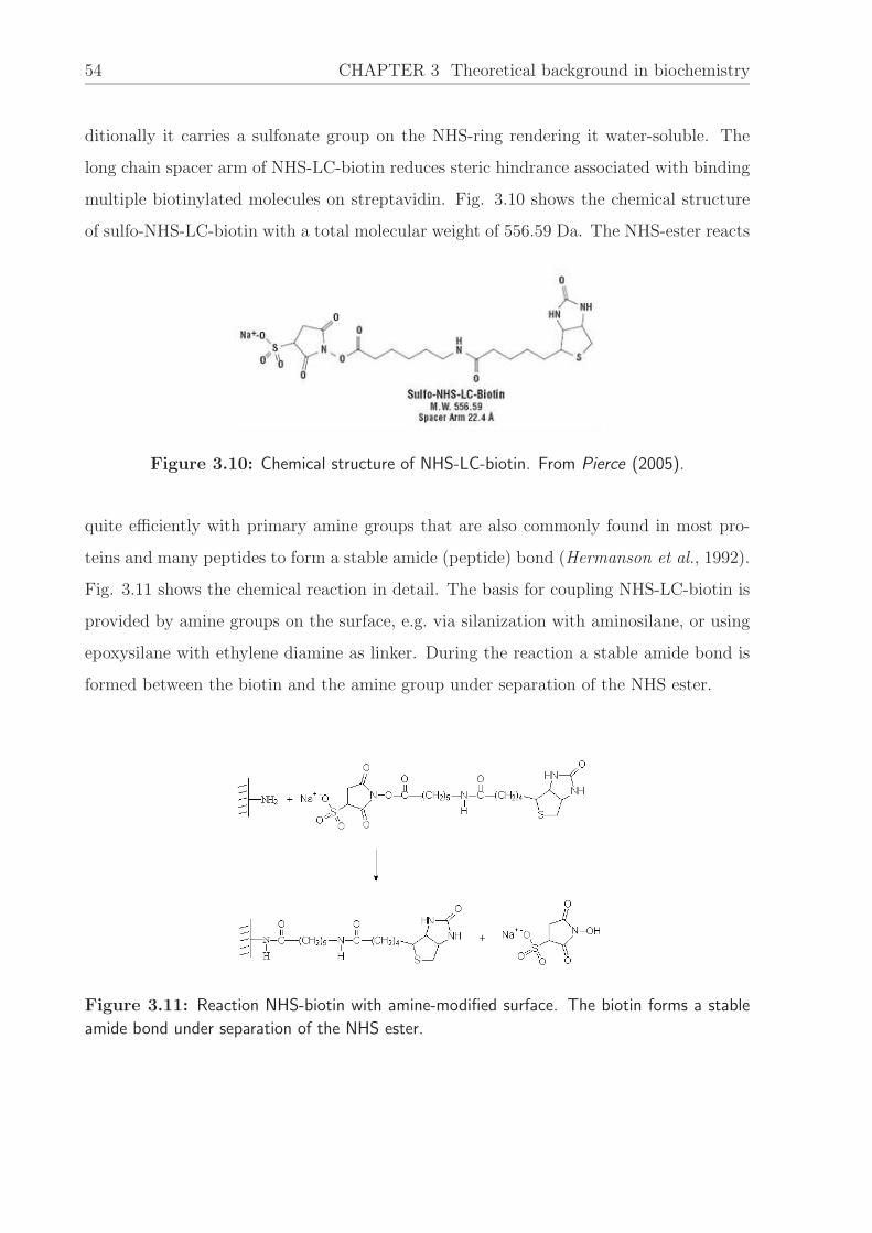
54 CHAPTER 3 Theoretical background in biochemistry
ditionally it carries a sulfonate group on the NHS-ring rendering it water-soluble. The
long chain spacer arm of NHS-LC-biotin reduces steric hindrance associated with binding
multiple biotinylated molecules on streptavidin. Fig. 3.10 shows the chemical structure
of sulfo-NHS-LC-biotin with a total molecular weight of 556.59 Da. The NHS-ester reacts
Figure 3.10: Chemical structure of NHS-LC-biotin. From Pierce (2005).
quite efficiently with primary amine groups that are also commonly found in most pro-
teins and many peptides to form a stable amide (peptide) bond (Hermanson et al., 1992).
Fig. 3.11 shows the chemical reaction in detail. The basis for coupling NHS-LC-biotin is
provided by amine groups on the surface, e.g. via silanization with aminosilane, or using
epoxysilane with ethylene diamine as linker. During the reaction a stable amide bond is
formed between the biotin and the amine group under separation of the NHS ester.
Figure 3.11: Reaction NHS-biotin with amine-modified surface. The biotin forms a stable
amide bond under separation of the NHS ester.

3.5 Biochemical background on the application measurement reagents 55
3.5.3 Cytochrome c
Cytochrome c is a small heme protein with a molecular weight of 12.4 kDa Lehninger
et al. (1994). This soluble protein consists of a single polypeptide chain and contains a
heme group. As an essential component of the mitochondrial respiratory chain, its main
function is the transfer of electrons, since it does not bind oxygen, but is capable of being
oxidized or reduced. Fig. 3.12 displays a three-dimensional model of cytochrome c, where
the functional heme group is shown in red.
Figure 3.12: Three-dimensional model of cytochrome c. The heme group is shown in red.
Adapted from Lehninger et al. (1994).
Cytochrome c is a very stable and well characterized molecule and therefore suited for
biosensor application measurements. We used biotinylated cytochrome c to monitor its
binding to a streptavidin-functionalized surface. The experiments will be further described
in chapter 5.

Chapter 4
Sensor design and characterization
4.1 Introduction
This section describes the setup of the interferometric biosensor implementing a two-
channel flow cell as fluidic element (IBS 201). The system is based on the optical principle
of a Young interferometer. A sketch of the setup is given on the next page.
The key component of the interferometric biosensor is the Ta2O5 transducer chip provided
by Unaxis Balzers, Liechtenstein. In the realized setup the radiation of a red light source
(several light sources have been tested, see below) is focused as a line on the first chip
grating and guided in two separate paths in a thin Ta2O5 film. One path serves as sensing
branch, where for example antibodies can be immobilized for antigen detection, the other
beam is used as reference branch. The two beams are coupled out by a second grating
and pass a double slit. On a CCD line sensor the resulting interference pattern can be
recorded.
When the analyte is added, i.e. binding molecules cause a local change in surface mass
coverage, the phase velocity of the light in the waveguide is decreased and the interference
pattern is laterally shifted. This shift is then further evaluated.
57
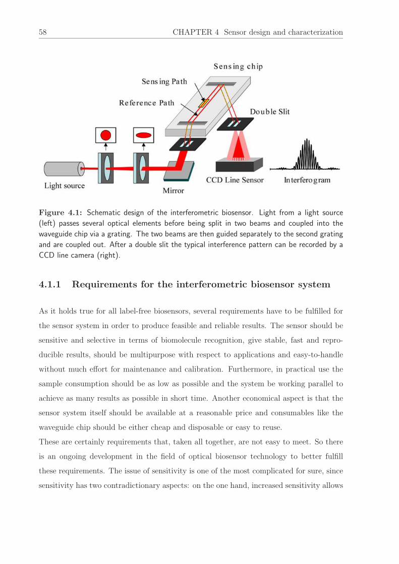
58 CHAPTER 4 Sensor design and characterization
Figure 4.1: Schematic design of the interferometric biosensor. Light from a light source
(left) passes several optical elements before being split in two beams and coupled into the
waveguide chip via a grating. The two beams are then guided separately to the second grating
and are coupled out. After a double slit the typical interference pattern can be recorded by a
CCD line camera (right).
4.1.1 Requirements for the interferometric biosensor system
As it holds true for all label-free biosensors, several requirements have to be fulfilled for
the sensor system in order to produce feasible and reliable results. The sensor should be
sensitive and selective in terms of biomolecule recognition, give stable, fast and repro-
ducible results, should be multipurpose with respect to applications and easy-to-handle
without much effort for maintenance and calibration. Furthermore, in practical use the
sample consumption should be as low as possible and the system be working parallel to
achieve as many results as possible in short time. Another economical aspect is that the
sensor system itself should be available at a reasonable price and consumables like the
waveguide chip should be either cheap and disposable or easy to reuse.
These are certainly requirements that, taken all together, are not easy to meet. So there
is an ongoing development in the field of optical biosensor technology to better fulfill
these requirements. The issue of sensitivity is one of the most complicated for sure, since
sensitivity has two contradictionary aspects: on the one hand, increased sensitivity allows
4.2 Interferometric biosensor: flow cell system 59
the detection of even lower concentrations of a molecule (or smaller molecules), on the
other hand the sensor system inevitably shows also an increased sensitivity to disturbing
factors like temperature fluctuations, technological imperfections, unspecific binding of
unwanted reactants and many more. These disturbing influences have to be compensated
for with optimization of the assay design and advanced technology. In the following the
design and realization of the interferometer system will be presented in detail taking these
aspects into account.
4.2 Interferometric biosensor: flow cell system
4.2.1 Biosensor setup - components
Light sources
During the development and especially for reasons of signal-to-noise (SNR) reduction
three different light sources have been tested and evaluated for their suitability. Initially
a helium-neon laser emitting at λ = 632.8 nm and a maximum output power of 3 mW
has been used. A laser source like a helium-neon has the advantage of being almost
monochromatic (∆λ = 0.1 nm). Another distinct feature of lasers is their very good
spatial and temporal coherence, therefore being well suited for interference experiments.
Yet the helium-neon laser is operated without temperature stabilization, rendering it more
sensitive to temperature fluctuations in the ambient resulting in wavelength fluctuations.
As described in chapter 2.7, wavelength fluctuations can lead to signal distortions when
the two beam pathways are of unequal length.
During most experiments described in this thesis, a superluminescent diode (SLD, λ =
675 nm, Superlum, Moscow) with a maxmimum output power of 3.5 mW served as light
source in the system. A SLD is essentially a semiconductor laser carrying antireflection
coatings on the end facets. Unlike lasers, it has no optical built-in feedback mechanism so
that lasing cannot occur. SLDs generally need operation with temperature stabilization.
The main reason for using the SLD in the interferometric system is the feature of partial
coherence due to its larger spectral bandwidth compared to a laser source, which allows
60 CHAPTER 4 Sensor design and characterization
the implementation of different evaluation algorithms for the interferogram signal, also
with respect to the development of the plate-reading system. One disadvantage of the SLD
has shown to be its incomplete linear polarization, requiring extra polarization measures
to allow guiding of proper TE or TM modes in the waveguide chip (see chapter 4.4.1).
For this reason, the suitability of a laser diode (λ = 670 nm, Sanyo, Japan) for the
interferometer system has been examined. In general, laser diodes have the advantages
of being quite small in size (5.6 mm package size) and reasonably priced, yet they are
temperature sensitive. Since in our experiments a laser diode with a maximum output
power of 7 mW was used, but only around 1.5 mW needed, possible heating of the diode
has been diminished by mounting it in a heat sink, without use of further temperature
stabilization.
Optical elements
For beamforming in front of the waveguiding chip, essentially two lenses have been im-
plemented (see also Fig. 4.1). Since all the light sources used have a certain angle of
divergence, an aspheric lens with a focal length of f1 = 8 mm is adjusted accordingly in
front of the light source to collimate the beam. This collimated beam is afterwards fo-
cused by a cylindrical lens with a focal length of f2 = 130 mm to form a line-shaped beam
on the first grating of the waveguide chip. Practically the grating can also be located
slightly out of focus in case of the IBS 201, since here focusing on the grating is only done
to couple in enough power which would otherwise be lost outside the chip holder. All
lenses used in the system were ordered from Thorlabs, USA and are made of BK7 glass
(n=1.52) coated with an antireflection coating to maximize power transmission and avoid
reflections back into the light source.
Chip mount
The chip mount for the IBS 201 is a special design and has been built at the IPM. It im-
plements several functions as illustrated in Fig. 4.3 and 4.4 and allows quick replacement
and adjustment of the waveguide chip. The light beam, focused to a line by the cylindrical
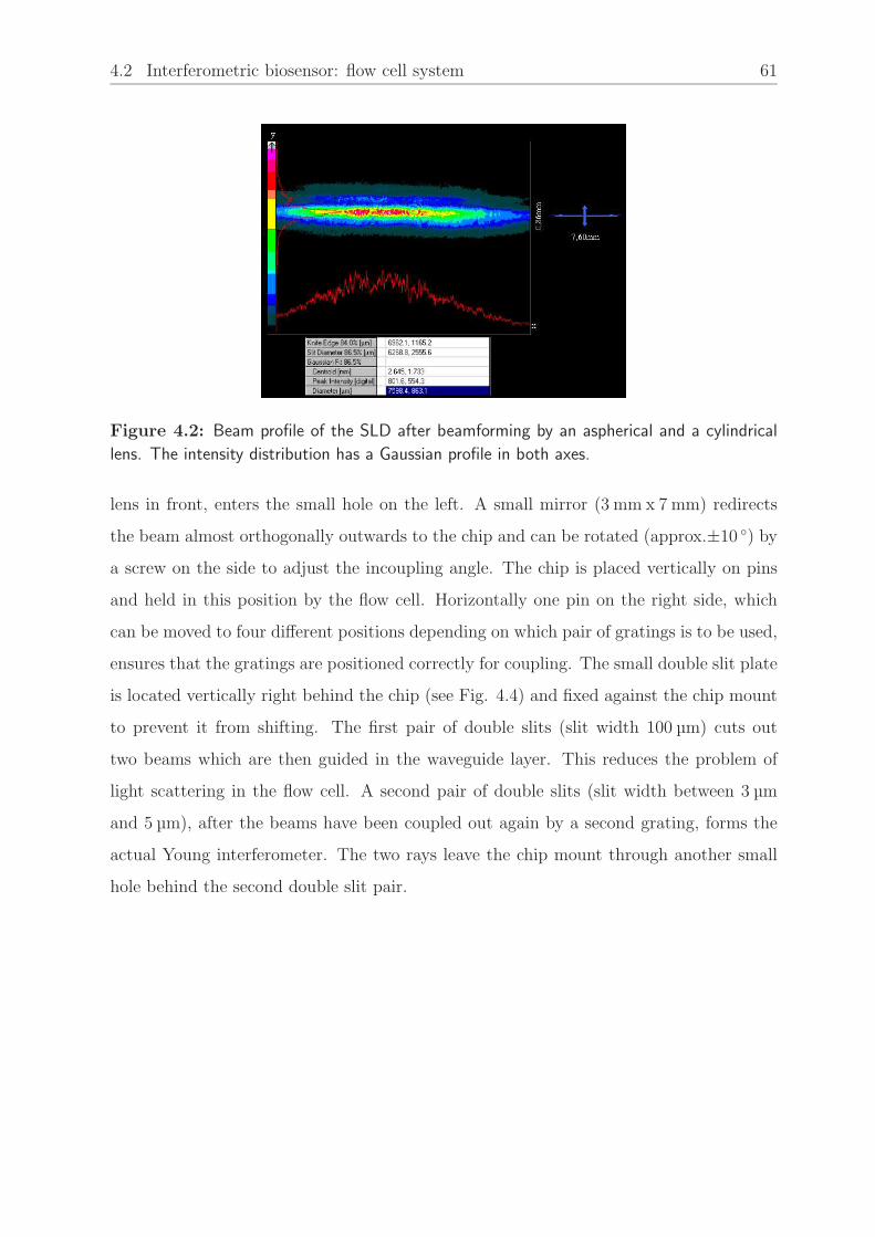
4.2 Interferometric biosensor: flow cell system 61
Figure 4.2: Beam profile of the SLD after beamforming by an aspherical and a cylindrical
lens. The intensity distribution has a Gaussian profile in both axes.
lens in front, enters the small hole on the left. A small mirror (3 mm x 7 mm) redirects
the beam almost orthogonally outwards to the chip and can be rotated (approx.±10 ) by
a screw on the side to adjust the incoupling angle. The chip is placed vertically on pins
and held in this position by the flow cell. Horizontally one pin on the right side, which
can be moved to four different positions depending on which pair of gratings is to be used,
ensures that the gratings are positioned correctly for coupling. The small double slit plate
is located vertically right behind the chip (see Fig. 4.4) and fixed against the chip mount
to prevent it from shifting. The first pair of double slits (slit width 100 µm) cuts out
two beams which are then guided in the waveguide layer. This reduces the problem of
light scattering in the flow cell. A second pair of double slits (slit width between 3 µm
and 5 µm), after the beams have been coupled out again by a second grating, forms the
actual Young interferometer. The two rays leave the chip mount through another small
hole behind the second double slit pair.

62 CHAPTER 4 Sensor design and characterization
Figure 4.3: Chip mount design (CAD drawing). The red line represents the beam path from
left to right. Light enters through a small hole on the left, is redirected by a small mirror,
adjustable for incoupling, coupled into the waveguide and coupled out again on the right in
direction of the CCD camera.
Figure 4.4: Photograph of the chip mount without the flow cell being mounted. The double
slit plate behind the waveguide chip is now visible as well as the pins for chip positioning.
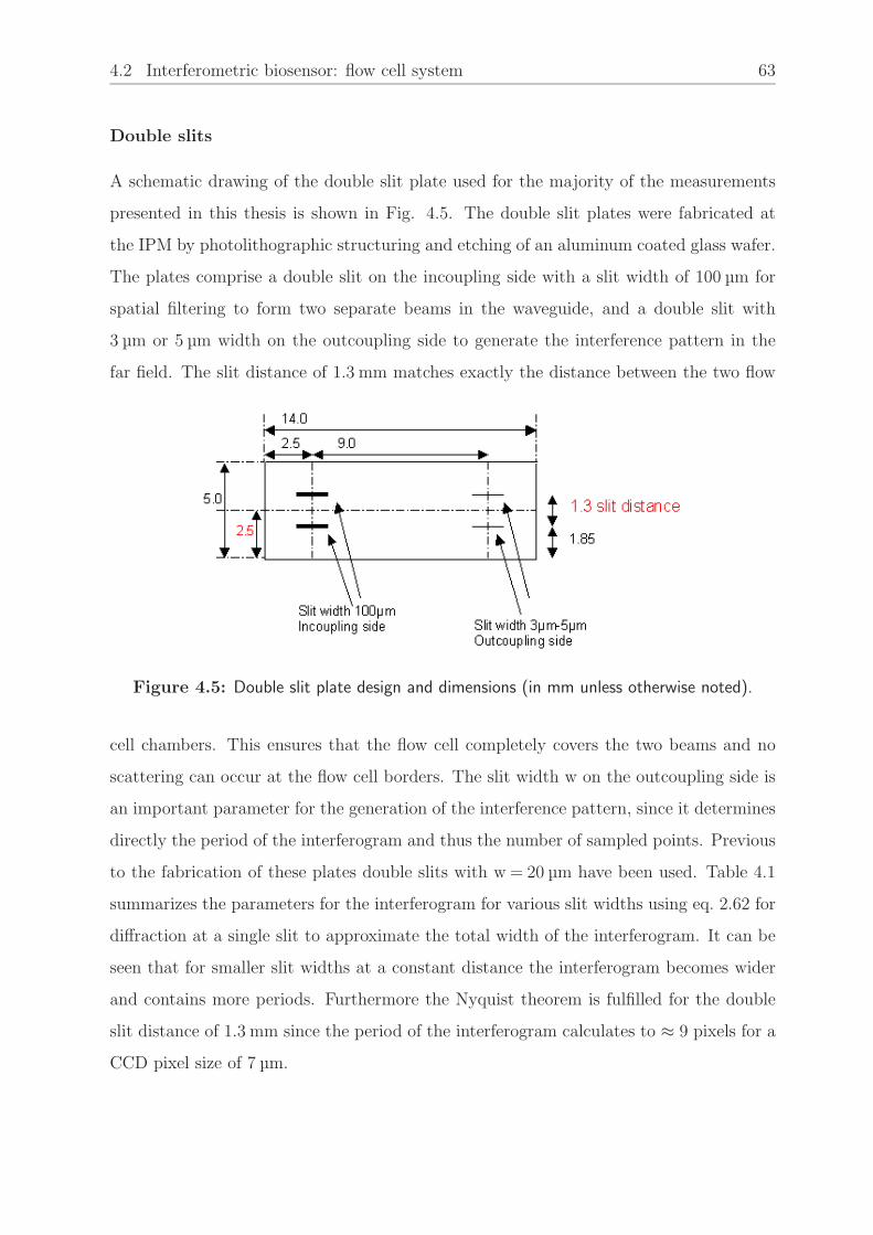
4.2 Interferometric biosensor: flow cell system 63
Double slits
A schematic drawing of the double slit plate used for the majority of the measurements
presented in this thesis is shown in Fig. 4.5. The double slit plates were fabricated at
the IPM by photolithographic structuring and etching of an aluminum coated glass wafer.
The plates comprise a double slit on the incoupling side with a slit width of 100 µm for
spatial filtering to form two separate beams in the waveguide, and a double slit with
3 µm or 5 µm width on the outcoupling side to generate the interference pattern in the
far field. The slit distance of 1.3 mm matches exactly the distance between the two flow
Figure 4.5: Double slit plate design and dimensions (in mm unless otherwise noted).
cell chambers. This ensures that the flow cell completely covers the two beams and no
scattering can occur at the flow cell borders. The slit width w on the outcoupling side is
an important parameter for the generation of the interference pattern, since it determines
directly the period of the interferogram and thus the number of sampled points. Previous
to the fabrication of these plates double slits with w = 20 µm have been used. Table 4.1
summarizes the parameters for the interferogram for various slit widths using eq. 2.62 for
diffraction at a single slit to approximate the total width of the interferogram. It can be
seen that for smaller slit widths at a constant distance the interferogram becomes wider
and contains more periods. Furthermore the Nyquist theorem is fulfilled for the double
slit distance of 1.3 mm since the period of the interferogram calculates to ≈ 9 pixels for a
CCD pixel size of 7 µm.

64 CHAPTER 4 Sensor design and characterization
Slit width w [µm] Period [µm] Width [mm] Contained periods
w p=λD/d B=2λD/w (B-d)/p
3 62.31 54 845.77
5 62.31 32.4 499.12
20 62.31 8.1 109.13
Table 4.1: Sample calculation for different double slit widths w with a detection distance of
D = 120 mm, slit separation d = 1.3 mm at λ = 675 nm
Waveguide chips
The core of the interferometric biosensor are the waveguide chips supplied by Unaxis
Balzers, Liechtenstein. A 16x48 mm glass wafer with five 0.5 mm wide etched gratings
(9 mm separation) is coated with a 154 nm film of Ta2O5. The gratings are covered by
an ≈ 500 nm thick and 4 mm wide protective layer of SiO2 leaving a 5 mm interaction
length for each of the four measurement positions. Fig. 4.6 shows the chip design and
dimensions, Fig. 4.7 illustrates the refractive index profile for a waveguide chip with the
relevant parameters given in Table 4.2.
Figure 4.6: Waveguide chip design and dimensions. A 154 nm thick Ta2O5 film is deposited
on a 16x48 mm glass wafer comprising five etched gratings. SiO2 layers protect the gratings
leaving a total interaction length of 5 mm.

4.2 Interferometric biosensor: flow cell system 65
substrate AF45 n=1.52 d=0.7 mm
waveguide Ta2O5 n=2.1 d=154 nm
covering layer SiO2 n=1.46 d≈500 nm
gratings period = 360 nm depth = 12-40nm coupling angle TE: −5.35
(with SiO2-layer: −3.574)
coupling angle TM: −15.422
(with SiO2-layer: −10.476)
evanescent field TE : FWHM=30.9 nm Pev.field
Ptot=11.27% TE: dneff
dtcover= 229 · 10−6 nm−1
TM : FWHM=37.9 nm Pev.field
Ptot=13.23% TM: dneff
dtcover= 439 · 10−6 nm−1
Table 4.2: Unaxis waveguide chip parameters. Calculations for λ=675 nm and ncover = 1.45.
b)a)
0,0
0,2
0,4
0,6
0,8
0,0 0,2 0,4 0,6 0,8 1,0
FWHM ev. field
waveguide
cover
normalized field distribution
heig
ht [µ
m]
-1,0 -0,8 -0,6 -0,4 -0,2 0,0 0,2 0,4 0,6 0,8 1,01,3
1,4
1,5
1,6
1,7
1,8
1,9
2,0
2,1
wave-guide
cover
substrate
refra
ctive inde
x n
waveguide thickness [µm]
Figure 4.7: a) Refractive index profile for a planar waveguide with refractive indices of
ns = 1.52, nf = 2.1, nc = 1.333 b) Field distribution in waveguide and cover at the same
parameters. The extension of the evanescent field is given as FWHM.
The coupling angles are given by the grating equation (Goodman, 1988):
neff = nc sinα +mλ
Λ(4.1)
with α being the coupling angle and Λ the grating period.
The extension of the evanescent field (given as FWHM, full width at half maximum),
the light intensity in the evanescent field and the sensitivity constants are calculated
according to (Tiefenthaler and Lukosz , 1989). The additional protective layer of SiO2
above the optical gratings represents an alteration to the supplied chips. These protective

66 CHAPTER 4 Sensor design and characterization
layers were fabricated at the IPM by ion assisted deposition (IAD) to ensure that the
flow cell never comes into contact with the evanescent field and thus prevents light from
scattering at the flow cell and disturbing the signal. Moreover, since the flow cell is made
of silicone and an equal and reproducible contact pressure is almost impossible to achieve,
the flow cell might alter its shape during a measurement and lead to signal drifts or other
distortions if it was not prevented to interact with the evanescent field. As the effective
thickness of the evanescent field is less than 100 nm for the given waveguide parameters
and wavelength, a thickness of ≈500 nm for the protective layers is sufficient. The inset
in Fig. 4.6 illustrates the effect of the protective layers on the waveguide film when a light
mode is guided.
Gratings with different diffraction grating depths were supplied by Unaxis with 12 nm,
22 nm, 30 nm and 40 nm and tested for their coupling characteristics and total power
transmission of the waveguide chip as described in the experimental section. Fig. 4.8
shows an atomic force microscope (AFM) picture of a diffraction grating in glass with a
grating depth of 12 nm.
Figure 4.8: Atomic force microscope (AFM) image of a diffraction grating in glass,
2 µm x 2 µm. The grating period is 318 nm and the grating depth is 12 nm. (Courtesy of
Unaxis)
Flow cell mount and flow cell
Both the flow cell mount and the flow cells have been constructed and fabricated at
the IPM and are a special design for the interferometric biosensor. Two types of flow
cells can be used according to the application: a two-channel flow cell as shown in the

4.2 Interferometric biosensor: flow cell system 67
photograph and the CAD design of the mounted flow cell in Fig. 4.9. A single-channel
flow cell covering both channels as shown in Fig. 4.10 allows a simultaneous application
of analyte solutions on differently immobilized channels and therefore referencing of for
example refractive index differences. The flow cells are made of two-component silicone-
based fluid (Sylgard 170, Corning, USA) which is formed and heat-treated to a flexible
flow cell shape. Over time, usually several months depending on the degree of usage, the
silicone deteriorates and the flow cell has to be renewed.
Figure 4.9: a) Photograph of the two-channel flow cell b) CAD design of the mounted flow
cell.
Figure 4.10: Photograph of the single-channel flow cell and its casting mold.
The two-channel flow cell has dimensions of ≈5.6 x 1.8 x 0.3 mm3 equating a volume of
≈3 µl per channel. The single channel flow cell has a volume of ≈3.5 µl with dimensions
of 6.9 x 1.7 x 0.3 mm3.
CCD camera
The device mainly used for signal detection was a CCD1000 (Stresing, Berlin, Germany)
with an integrated ILX 526A sensor (Sony, Tokyo, Japan). A CCD is basically a semi-
conductor chip sensitive to light and subdivided into many discrete rectangular areas

68 CHAPTER 4 Sensor design and characterization
called pixels. Each photon impinging on a pixel results in a charge, which is accumu-
lated for all photons within the exposure time and stored for readout as a measurable
voltage signal. The ILX526A sensor is a line sensor comprising 3200 pixels at a pixel
size of 7 µm x 200 µm. The camera is usually used at exposure times between 50 ms and
250 ms for experiments. Previously the same camera, but with an ILX 511 line sensor
(2048 pixels, pixel size 14 µm x 200 µm) has been used. Further, a full-line binned CCD
(Hamamatsu, Japan) comprising a total number of pixels of 2048 x 14 with a pixel size of
14 µm x 14 µm has been tested.
Peristaltic pump
A peristaltic pump (Ismatec, Wertheim, Germany) installed externally allows continuous
pumping of analyte solutions in up to four channels through the system. All required tub-
ing is obtained from Novodirect, Kehl, Germany. Silicone tubing with an inner diameter
of 0.5 mm has proven suitable as well as outlet tubing of silicone with an inner diameter of
0.64 mm. Silicone has the advantage of being biocompatible and chemically inert to most
buffers used during the experiments. For biological applications it is advisable to renew
the inlet tubing previous to a new measurement run. Since the two channels can be used
either as sensing path or as reference path, it is not necessary to predefine the channels.
Dragging of the liquids through the system instead of pumping seems more advantageous,
because in this configuration the inlet tubing can be chosen very short and thus mixing of
sample liquids is reduced. The pumping velocity is programmable, as standard velocity
the setting 0.10 ml/min on the pump, being equal to an effective velocity of ≈80 µl/min
per channel for the given tubing configuration, was chosen. With ≈20 cm inlet tubing
length this corresponds to a response time of the system of around 30 sec.
4.2.2 Biosensor setup - realization
This section describes the realized setup of the interferometric biosensor implementing
the components introduced above. The system setup has to meet certain requirements,
such as being robust, compact and adjustable without major efforts. Fig. 4.11 illustrates

4.2 Interferometric biosensor: flow cell system 69
the current setup of the flow cell instrument in top view. Light from the light source (1)
is collimated by an aspherical lens with f=8 mm (2) and passes a polarizer (3) for linear
polarization. Several optical density filters from 0.1 to 2 (4) decrease the light intensity if
necessary. A cylindrical lens focuses the collimated beam onto the waveguide chip grating.
The complete chip holder and the fluidics are hidden behind the black lid (6), which can
be opened separately to access these components. An optional cylindrical lens (7) allows
refocusing onto the CCD line sensor (8), depending on available light intensity coming
out of the waveguide chip. The CCD camera (9) transmits the recorded data from the
sensor to a PCI card in a computer connected to the system where the data are processed
by an FFT algorithm.
Figure 4.11: Functional design of the interferometric biosensor IBS 201. Refer to the text
for the meaning of the numbered components.
Figure 4.12: Front view photograph of the interferometric biosensor IBS 201.
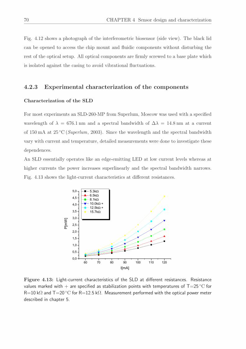
70 CHAPTER 4 Sensor design and characterization
Fig. 4.12 shows a photograph of the interferometric biosensor (side view). The black lid
can be opened to access the chip mount and fluidic components without disturbing the
rest of the optical setup. All optical components are firmly screwed to a base plate which
is isolated against the casing to avoid vibrational fluctuations.
4.2.3 Experimental characterization of the components
Characterization of the SLD
For most experiments an SLD-260-MP from Superlum, Moscow was used with a specified
wavelength of λ = 676.1 nm and a spectral bandwidth of ∆λ = 14.8 nm at a current
of 150 mA at 25 C (Superlum, 2003). Since the wavelength and the spectral bandwidth
vary with current and temperature, detailed measurements were done to investigate these
dependences.
An SLD essentially operates like an edge-emitting LED at low current levels whereas at
higher currents the power increases superlinearly and the spectral bandwidth narrows.
Fig. 4.13 shows the light-current characteristics at different resistances.
60 70 80 90 100 110 1200,0
0,5
1,0
1,5
2,0
2,5
3,0
3,5
4,0
4,5
5,0
P[m
W]
I[mA]
5.3k 6.5k 8.1k 10.0k + 12.5k + 15.7k
Figure 4.13: Light-current characteristics of the SLD at different resistances. Resistance
values marked with + are specified as stabilization points with temperatures of T=25 C for
R=10 kΩ and T=20 C for R=12.5 kΩ. Measurement performed with the optical power meter
described in chapter 5.

4.2 Interferometric biosensor: flow cell system 71
The measurement shows a superlinear power-current dependence and an increasing power
at higher resistances, i.e. lower thermistor temperatures. Due to the fact that the SLD
should be operated at high power to obtain a high light intensity and the highest stable
resistance is specified for 12.5 kΩ, this resistance value was chosen for all experiments.
Another crucial parameter is the spectral bandwidth of the light source, since it directly
correlates with the coherence length and thus influences the interference pattern. The
corresponding test series (Fig. 4.14) shows the dependences of wavelength and spectral
bandwidth on current or resistance. Extrapolation of the obtained data yields for a re-
sistance of 12.5 kΩ and a current of 100 mA a wavelength of λ=675.5 nm and a spectral
bandwidth of ∆λ=10.35 nm which is in good accordance with the specifications.
dc
ba
60 80 100 120 140 160
676,0
676,5
677,0
677,5
678,0
678,5
679,0
679,5
λ [n
m]
Current [mA]8000 8500 9000 9500 10000
676,4
676,6
676,8
677,0
677,2
677,4
677,6
677,8
λ [n
m]
Resistance [ ]
8000 8500 9000 9500 1000011,1
11,2
11,3
11,4
11,5
11,6
11,7
11,8
11,9∆λ
[nm
]
Resistance [ ]
60 80 100 120 140 160
11
12
13
14
15
16
17
18
19
20
∆λ [n
m]
Current [mA]
Figure 4.14: Wavelength-current and wavelength-resistance characteristics of the SLD.
a) Spectral bandwidth ∆λ versus diode current at a constant resistance of 9 kΩ
b) Spectral bandwidth ∆λ versus thermistor resistance at a constant current of 100 mA (red
line denotes linear fit)
c) Wavelength versus diode current at a constant resistance of 9 kΩ (red line denotes linear
fit)
d) Wavelength versus thermistor resistance at a constant current of 100 mA (red line denotes
fit to an exponential decay model of power 2.

72 CHAPTER 4 Sensor design and characterization
The fundamental correlation between coherence length and spectral bandwidth is de-
scribed by the following expression (Kuhlke, 2004):
∆f ≈ 1
τc
=c0
lc(4.2)
i.e. the larger the spectral bandwidth of the light source, the smaller the coherence time
(and coherence length, respectively). Eq. 4.2 can be expanded to obtain a relationship
between the wavelength and the coherence length:
∆f =∂f
∂λ∆λ
= − c0
λ2∆λ
⇒ lc =λ2
∆λ(4.3)
With the given values for wavelength and spectral bandwidth the theoretical coherence
length of the SLD can be determined to lc = 44 µm. Experimentally the coherence length
can be derived from the coherent region of the interference pattern, as shown in Fig. 4.15
according to:Bc
p=
lcλ
(4.4)
0 500 1000 1500 2000 2500 30000
1000
2000
3000
4000
inte
nsity
pixel
Figure 4.15: Interferogram from a double-slit experiment recorded with the SLD in TM
mode as light source.

4.2 Interferometric biosensor: flow cell system 73
where Bc
pis given by the number of periods p in the coherent region Bc. From the
interferogram a total number of periods of ≈50 is obtained, yielding a coherence length
of ≈33 µm which is in good accordance with the theoretical value.
Characterization of the laser diode
As alternative light source for the interferometric biosensor a laser diode can be imple-
mented. Laser diodes have the advantages of being compact and small sized, however
they are very sensitive to back reflections. Like all lasers, laser diodes have the feature of
operating like an LED below a certain threshold current, therefore emitting semicoherent
light in this case. Above threshold current these light sources are characterized by a high
degree of coherence and linearity between output power and input current. For the in-
terferometric biosensor, especially the power range below threshold current is interesting
due to the semicoherence feature. Fig. 4.16 shows the light-current characteristics of a
Sanyo DL3149 laser diode (Sanyo, Japan) with a peak wavelength of λ = 670 nm. The
threshold current has been determined to 25 mA, the slope efficiency above threshold to
308 µW/mA.
0 5 10 15 20 25 30 35 40
0
500
1000
1500
2000
2500
3000
3500
4000
P [µ
W]
I [mA]
Figure 4.16: Light-current characteristics of the Sanyo DL3149 laser diode operated without
temperature stabilization. The threshold current is 25 mA, the slope efficiency has been
determined to 308 µW/mA. Measurement performed with the optical power meter described
in chapter 5.

74 CHAPTER 4 Sensor design and characterization
Despite the fact that this type of laser diode has a comparatively high threshold current,
the available power right below threshold is only ≈100 µW. In this case the remaining
low light intensity on the CCD has to be compensated with higher exposure times. In
addition, this laser diode is not temperature stabilized in contrast to the SLD, so that the
SLD remains the preferred light source for our applications.
Characterization of different CCD sensors
The camera system used for the interferometric biosensor is the CCD1000 where different
sensors have been integrated and tested concerning dark current and signal-to-noise. A
high signal-to-noise ratio is important for the signal evaluation, since pixel noise directly
correlates with phase noise, as will be shown in section 4.2.5. Dark current measurements
have been performed with all three sensors described in Table 4.3.
Sony ILX 511 Sony ILX 526A Hamamatsu S9840
no. of pixels 2048 3200 2048 x 14
pixel size 14 x 200 µm (14 µm pitch) 7 x 200 µm (7 µm pitch) 14 x 14 µm
sensor length 28.67 mm 21 mm 28.67 mm
Table 4.3: Comparison of the CCD sensors used for the interferometric biosensor
Fig. 4.17 summarizes the results for exposure times for up to 800 ms. The results show
a significantly lower dark current noise for the arrayed sensor than for the line sensors
at comparable exposure times. Based on these findings it was expected that the signal
noise should also be lower for the arrayed sensor, resulting in an increased signal-to-noise
ratio. Thus another measurement was performed investigating the signal noise dependent
on the gray value. For this, the SLD was collimated by the aspheric lens and the signal
intensity on the camera varied by either varying the driving current of the SLD or the
exposure time. The results are illustrated in Fig. 4.18. As expected, the arrayed sensor
shows a significantly lower signal noise at comparable gray values than the other sensors.
A simulation has been performed to study the correlation of pixel noise and phase noise,
and a linear dependence thereof can be observed (see Fig. 4.19. Thus it is expected that
the implementation of the arrayed sensor should yield the lowest phase noise.
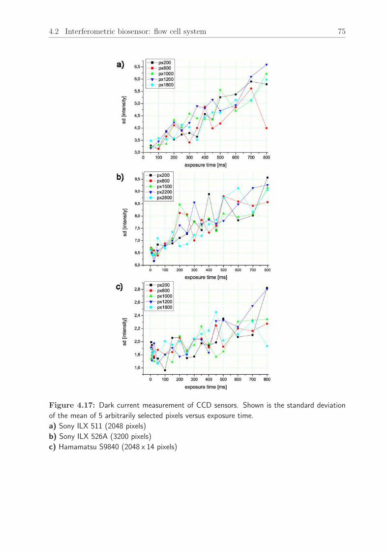
4.2 Interferometric biosensor: flow cell system 75
Figure 4.17: Dark current measurement of CCD sensors. Shown is the standard deviation
of the mean of 5 arbitrarily selected pixels versus exposure time.
a) Sony ILX 511 (2048 pixels)
b) Sony ILX 526A (3200 pixels)
c) Hamamatsu S9840 (2048 x 14 pixels)

76 CHAPTER 4 Sensor design and characterization
c)
b)
a)
0 500 1000 1500 2000 2500 3000 35000
1
2
3
4
5
6
7
8
9
Model: Y = A+B*sqrt(X)
A -1.32 ±0.19B 0.16 ±0.01
R2 0.91735
sd [i
nten
sity
]
mean [intensity]
Variation of exposure time Variation of SLD driving current
0 500 1000 1500 2000 2500 3000 35000
5
10
15
20
25
Model: Y=A+B*sqrt(X) A 2.42 ±0.31B 0.40 ±0.01
R2 0.97982
Variation of exposure time Variation of SLD driving current
sd [i
nten
sity
]
mean [intensity]
0 500 1000 1500 2000 2500 3000 35000
2
4
6
8
10
12
14
16
18
Model: Y=A+B*sqrt(X) A 1.27 ±0.54B 0.24 ±0.02
R2 0.89349
Variation of exposure time Variation of SLD driving current
sd [i
nten
sity
]
mean [intensity]
Figure 4.18: Signal noise measurement of CCD sensors. Shown is the standard deviation of
the mean of 5 arbitrarily selected pixels versus the mean intensity.
a) Sony ILX 511 (2048 pixels)
b) Sony ILX 526A (3200 pixels)
c) Hamamatsu S9840 (2048 x 14 pixels)
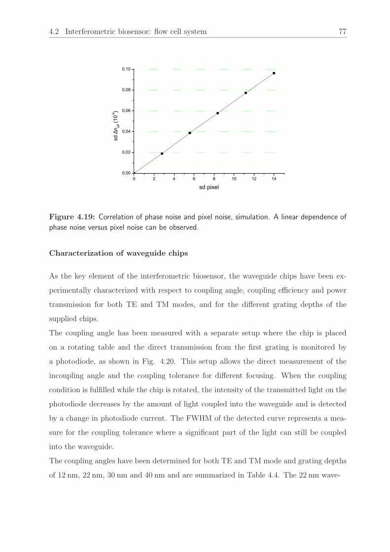
4.2 Interferometric biosensor: flow cell system 77
0 2 4 6 8 10 12 140,00
0,02
0,04
0,06
0,08
0,10
sd ∆
n eff (10
-6)
sd pixel
Figure 4.19: Correlation of phase noise and pixel noise, simulation. A linear dependence of
phase noise versus pixel noise can be observed.
Characterization of waveguide chips
As the key element of the interferometric biosensor, the waveguide chips have been ex-
perimentally characterized with respect to coupling angle, coupling efficiency and power
transmission for both TE and TM modes, and for the different grating depths of the
supplied chips.
The coupling angle has been measured with a separate setup where the chip is placed
on a rotating table and the direct transmission from the first grating is monitored by
a photodiode, as shown in Fig. 4.20. This setup allows the direct measurement of the
incoupling angle and the coupling tolerance for different focusing. When the coupling
condition is fulfilled while the chip is rotated, the intensity of the transmitted light on the
photodiode decreases by the amount of light coupled into the waveguide and is detected
by a change in photodiode current. The FWHM of the detected curve represents a mea-
sure for the coupling tolerance where a significant part of the light can still be coupled
into the waveguide.
The coupling angles have been determined for both TE and TM mode and grating depths
of 12 nm, 22 nm, 30 nm and 40 nm and are summarized in Table 4.4. The 22 nm wave-

78 CHAPTER 4 Sensor design and characterization
Figure 4.20: Setup for the determination of the coupling angles. The chip is placed on a
rotating table and the direct transmission from the first grating monitored by a photodiode
for angle intervals of 0.5 . The focal length of the cylindrical lens can be varied.
TE TM
12 nm 5.10 15.0
22 nm1 3.40 9.90
30 nm 5.23 14.95
40 nm 5.45 15.35
Table 4.4: Coupling angles for TE and TM and different grating depths. 1: the 22 nm
waveguide chips were already coated with the SiO2-layer at the time of measurement.
guide chips were already coated with the SiO2-layer at the time of measurement.
The averaged FWHM of all measurements depending on grating depth and focal length of
the cylindrical lens determine the coupling tolerance as shown in Fig. 4.21 for TE mode.
An optimal focal length for incoupling appears to be f=100 mm, independent of the grat-
ing depth. This result can be interpreted using eq. 4.1 and calculating the coupling angles
taking the spectral bandwidth of the SLD into account, which yields a required tolerance
of ≈±1 to couple the complete spectrum. With a given beam diameter of 3.5 mm for
TE mode this results in a required focal length of ≈100 mm.
Another crucial point is the total coupling efficiency of the waveguide chip, since the
output power is eventually detected by the CCD camera and therefore needs to be suf-
ficiently high. Power measurements were carried out for TE mode for the transmission
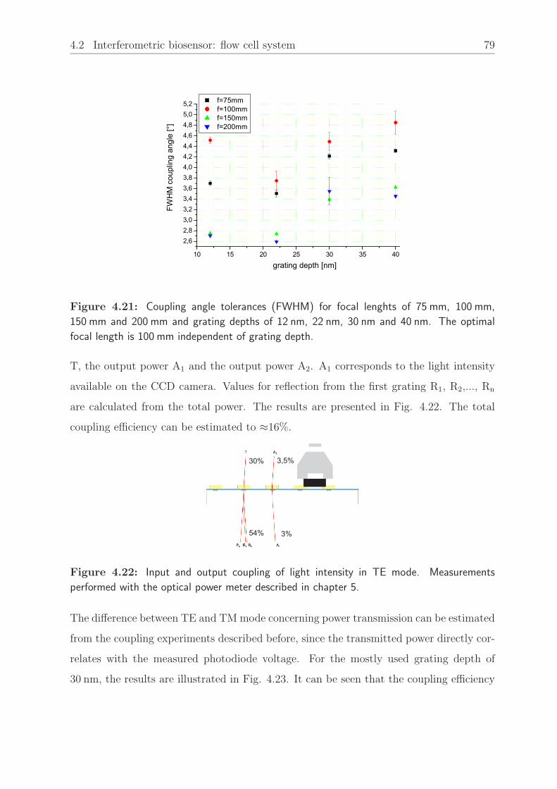
4.2 Interferometric biosensor: flow cell system 79
10 15 20 25 30 35 40
2,62,83,03,23,43,63,84,04,24,44,64,85,05,2 f=75mm
f=100mm f=150mm f=200mm
FWHM
cou
plin
g an
gle
[°]
grating depth [nm]
Figure 4.21: Coupling angle tolerances (FWHM) for focal lenghts of 75 mm, 100 mm,
150 mm and 200 mm and grating depths of 12 nm, 22 nm, 30 nm and 40 nm. The optimal
focal length is 100 mm independent of grating depth.
T, the output power A1 and the output power A2. A1 corresponds to the light intensity
available on the CCD camera. Values for reflection from the first grating R1, R2,..., Rn
are calculated from the total power. The results are presented in Fig. 4.22. The total
coupling efficiency can be estimated to ≈16%.
3 0 % 3 , 5 %
3 %5 4 %
3 0 % 3 , 5 %
3 %5 4 %
w w w w w ww w w w
Figure 4.22: Input and output coupling of light intensity in TE mode. Measurements
performed with the optical power meter described in chapter 5.
The difference between TE and TM mode concerning power transmission can be estimated
from the coupling experiments described before, since the transmitted power directly cor-
relates with the measured photodiode voltage. For the mostly used grating depth of
30 nm, the results are illustrated in Fig. 4.23. It can be seen that the coupling efficiency

80 CHAPTER 4 Sensor design and characterization
is about three times higher for TE mode than for TM mode. Yet also in TM mode
operation the light intensity is sufficient for signal detection.
-15 -10 -5 0 5 10 159,0
9,1
9,2
9,3
9,4
9,5
9,6
9,7
9,8b)
phot
odio
de v
olta
ge [m
V]
angle [°]-10 -8 -6 -4 -2 0 2 4 6 8 10
7,0
7,5
8,0
8,5
9,0
9,5
10,0
a)
phot
odio
de v
olta
ge [m
V]
angle [°]
Figure 4.23: Comparison of coupling efficiencies for TE and TM mode. a) Measurement
diagram for TE mode coupling. b) Measurement diagram for TM mode coupling.
4.2.4 Signal analysis and processing
This section presents an overview on the signal analysis software based on the Fourier
Transform described in chapter 2.6, and further signal processing steps and their evalua-
tion regarding a refining of the signal.
Fast Fourier Transform algorithm
A software algorithm environment in LabView™ based on a Fast Fourier Transform of
the interferogram has been designed for the interferometric biosensor. A detailed descrip-
tion of the Fourier Transform analysis of a fringe pattern can be found in (Kujawinska
and Wojciak , 1991). Several calculation-intensive parts of the algorithm have been pro-
grammed as C++ subroutines and are implemented as dynamic link library (DLL) to
work with the Labview™ interface.
The starting point of the signal analysis is the signal itself, here an interferogram. The
CCD camera samples images with a predefined exposure time that are displayed on a
customized LabView™ user interface. Depending on the CCD sensor either 2000 or 3000
pixels are displayed. The region of interest depends on the coherent area within the inter-

4.2 Interferometric biosensor: flow cell system 81
ference pattern and thus on the light source characteristics. Fig. 4.24 shows an example
of an interferogram sampled by the ILX 526A sensor and the corresponding region of
interest.
b)a)
1000 1100 1200 1300 1400 1500 16001000
1500
2000
2500
3000
3500
4000
inte
nsity
pixel
0 500 1000 1500 2000 2500 30000
1000
2000
3000
4000
inte
nsity
pixel
Figure 4.24: a) Interferogram recorded by the CCD camera (3000px) b) The region of
interest (i.e. coherent area of the interferogram) from a)
Before the actual FFT is applied to the signal, the sampling properties of the CCD have
to be investigated to ensure that the Nyquist Theorem (see ch. 2.6) is fulfilled for a correct
transform. The pixel sizes of the CCD sensors vary from 7 µm to 14 µm, so that every
7 µm or 14 µm the interferogram is sampled (sampling period). This results in a sampling
frequency of fs=1/7 µm−1 or fs=1/14 µm−1. From Fig. 4.24b an interferogram period
of ≈9 pixels can be determined, equivalent to 63 µm or 126 µm, respectively. Thus the
maximum interferogram frequency is 1/63 µm−1. The Nyquist Theorem states that the
sampling frequency must be greater than twice the frequency of the signal being sampled,
and with 1/14 ≥ 2 ∗ 1/63 this requirement is fulfilled and there should be no error due to
aliasing for the current interferometer setup.
The sampled signal then undergoes an FFT in order to accurately estimate the spatial
period of the interferogram and thus the spatial frequency which corresponds to the max-
imum of the signal peak of the FFT (see Fig. 4.25). However, the FFT does not give any
information on possible distortions of the signal peak, and, due to discretization, the true
signal peak probably lies between two discrete data points in the FFT spectrum. One
way to improve the estimation accuracy of the signal peak is zeropadding of the sampled

82 CHAPTER 4 Sensor design and characterization
signal, thereby increasing the resolution in the FFT response by linear interpolation. De-
tails on the effects of zeropadding will be described in the following subsection.
0,0 0,1 0,2 0,3 0,4 0,50
60
120
180
Frequency
Ampl
itude
-200000-150000-100000-50000
00,0 0,1 0,2 0,3 0,4 0,5
Frequency
angl
e [°
]
Figure 4.25: FFT Plot of the interferogram signal from Fig. 4.24.
After determination of the spatial frequency of the interferogram, the corresponding phase
value is extracted from the FFT spectrum and passed to a routine to calculate ∆neff . The
phase values are obtained in phase fringes (phase modulo 2π) and have to be unwrapped
to get a continuous phase information, i.e. when a discontinuity is detected by the software
routine, 2π are added or subtracted. Both phase values and ∆neff values are displayed
on the user interface in real-time and stored in a datafile for post-processing, e.g. with
Origin©. Note that in the following “phase“and “∆neff“are used interchangeably, since
they are related through a simple scalar multiplication. A flowchart and a snapshot of
the current user interface of the FFT software routine can be found in Appendix D.
Signal processing - zeropadding
Recall from chapter 2.6 that for an effective application of an FFT the signal length has to
be a power of two, which can be accomplished by extending the signal with trailing zeros.
Extending the original signal with more trailing zeros than the next power of two leads
to a linear interpolation of the discrete data points in the spectrum of the FFT and thus
a more accurate determination of the signal peak corresponding to the spatial frequency.

4.2 Interferometric biosensor: flow cell system 83
The question is, if a more accurate determination of the spatial frequency results in a
more accurate phase value and thus less phase noise. Fig. 4.26 illustrates this difference
0,170 0,175 0,180 0,185 0,190 0,195 0,200
0,00
0,01
0,02
0,03
0,04
0,05
0,06
0,07b)
∆f=0.0000019
Am
plitu
de
Frequency0,170 0,175 0,180 0,185 0,190 0,195 0,200
0
20
40
60
80
∆f=0.000244
a)
Am
plitu
de
Frequency
Figure 4.26: Influence of zeropadding on the FFT signal peak. The FFT was applied to the
interferogram signal from Fig. 4.24 with an original signal length of 3200 pixels. a) Extension
of the original signal to effectively 4096 pixels resulting in ∆f=0.000244 with fmax = 0.186035.
b) Extension of the original signal to effectively 524288 pixels resulting in ∆f=0.0000019 with
fmax = 0.1861629.
where the FFT has been applied to the interferogram signal from Fig. 4.24 with an original
signal length of 3200 pixels (CCD readout). In the first case, the signal is extended to
effectively 4096 pixels (212), in the second case to effectively 524288 pixels (219). Due to
the linear interpolation, the signal peak can be determined more accurately in the second
case. However, a better estimation of the true spatial frequency does not necessarily lead
to an improvement in phase noise, as the next figure shows. The phase trends differ
slightly in their absolute values, while the phase noise remains the same. In summary,
the implementation zeropadding seems useful for an efficient FFT calculation and a more
accurate estimation of the spatial frequency, whereas an improvement in phase noise
cannot be observed.

84 CHAPTER 4 Sensor design and characterization
Figure 4.27: Influence of zeropadding on the phase trend. No improvement of phase noise
due to a more accurate determination of the spatial frequency by zeropadding can be observed.
Adapted from (MacKenzie, 2003).
Signal processing - averaging
Recall from chapter 2.7.3 the two types of average filters implemented into the software
algorithm - block average and moving average. Whereas the block average reduces the
sampling rate by the averaging factor n, the recursive moving average filter maintains a
constant buffer size without altering the sampling rate. Another effect of averaging is a
reduction in signal noise according to:
σ ∝ 1√n
(4.5)
where σ denotes the phase noise.
Fig. 4.28 shows the results of a simulation of phase trends filtered by block or moving
average or both.
The results show an equal reduction in phase noise for both filtering methods. However,
when both filters are applied simultaneously, no further noise reduction can be observed.
Thus both filtering methods can be recommended to accomplish phase noise reduction
in the interferometer system. Yet a few things have to be considered before strongly
averaging the signal: both filters do not only influence the phase trend by reducing the
peak-to-peak noise, but also have long-term effects. Since the block average filter reduces

4.2 Interferometric biosensor: flow cell system 85
0 20 40 60 80 100 1200,0
0,2
0,4
0,6
0,8
1,0 Moving average filter Block average filter Moving average + block average filter Theory
phas
e no
ise
(norm
aliz
ed)
averaging factor N
Figure 4.28: Simulation of phase noise reduction by averaging, normalized.
the sampling rate by the averaging factor n, the time resolution of the measurement
is consequently reduced by the same factor. For example, given an exposure time of
τ=200 ms and a block averaging factor of n=5, the resulting sampling rate T is given by:
T = τ · n (4.6)
i.e. reduced from 5 Hz to only 1 Hz. For most applications of the interferometric biosensor,
it is recommended that the sampling rate does not fall below 1 Hz, corresponding to
maximum averaging factors of n=16 or n=32, depending on the chosen exposure time.
The moving average filter also influences the long-term phase trend, but in a different way.
Since here the oldest value in the buffer is constantly replaced by the newly measured
one, each averaged phase value is influenced by all values in the buffer. This fact has
to be considered especially for reaction kinetics measurements, where a short-term phase
change determines kinetic rate constants and a large buffer size would lead to distorted
phase values. Therefore the same recommendation applies for the moving average filter,
that the averaging factor, i.e. buffer size, should not exceed 16-32 resulting in a sampling
rate of ≈1 Hz.

86 CHAPTER 4 Sensor design and characterization
4.2.5 Experimental characterization of the biosensor system
Refractive index measurements
Since the principle of evanescent field sensing can be used to detect changes in the bulk re-
fractive index of a cover fluid, refractive index measurements were performed with glycerin
dilutions in order to test and calibrate the system with respect to its physical characteris-
tics, i.e. signal noise, signal drift and sensitivity constants. Glycerin has been the sample of
choice due to its low cost, neutrality and easy handling. All measurements were prepared
and performed as follows:
• A sufficient amount of DI − H2O (≈150 ml) is degassed for at least 1 h. This reduces
built-up of air bubbles in the fluidic system that could disturb the measurement
• Preparation of a stock solution of 10 % (w/v) glycerin in degassed DI − H2O (cor-
responds to 793 µl glycerin per 10ml DI − H2O)
• Preparation of glycerin dilutions from the stock solution in the range of 0.5 % to
5 % (w/v) in separate reaction vessels
• The interferometer system is prepared by connecting inlet- and outlet tubing, insert-
ing a clean waveguide chip, starting the peristaltic pump and monitoring a baseline
with DI − H2O on both channels
• All system parameters like exposure time, SLD current and averaging should be
reasonably set (typical values: t = 100-400 ms, I = 100-120 mA and averaging 2-10)
When a stable baseline with a drift of less than 1 · 10−6 in ∆neff is reached, the measure-
ment can be started by pausing the pump for placing the inlet tubing of the measurement
channel into the reaction vessel containing the lowest glycerin concentration, resuming
pumping, changing back to H2O, and applying the same concentration at least three
times to check on repeatability and stability of the signal change, and then move on to
the next higher concentration. Typical time intervals for applying the samples are be-
tween two and four minutes, followed by running buffer (in this case DI − H2O) for the
same time interval, while the reference channel is continuously kept under running buffer.

4.2 Interferometric biosensor: flow cell system 87
Fig. 4.29 presents a measurement of glycerin solutions from 1 % to 5 % (w/v) based on
this measurement procedure with the SLD in TE mode as light source.
0 10 20 30 40 50 60
0
100
200
300
400
5%
4%
3%
2%
1%
∆nef
f (10
-6)
time [min]
Figure 4.29: Refractive index measurement with glycerin solutions from 1 % to 5 % (w/v)
as sample with the SLD in TE mode as light source. Measurement parameters: R=12.5 kΩ,
I=120 mA, τ=250 ms.
0,001 0,002 0,003 0,004 0,005 0,0060,00005
0,00010
0,00015
0,00020
0,00025
0,00030
0,00035
0,00040
0,00045
0,00050
Linear Regression Y = A + B * XWeight given by error bars
A -8.72*10-6 ± 1.11*10-6
B 0.08027 ± 2.6*10-4
R2 0.99979
Theoretical value for B: 0.08195
∆nef
f
∆n0
Figure 4.30: Calibration curve derived from glycerin concentration measurements for TE
mode. The mean signal change in ∆neff for each concentration is plotted versus the refractive
index n. From the slope of the linear fit the sensitivity constant can be determined to∆neff
∆n0=
0.08027.

88 CHAPTER 4 Sensor design and characterization
Fig. 4.30 shows the calibration curve corresponding to this measurement, where the mean
signal change in ∆neff for each concentration is plotted versus the refractive index n ob-
tained from literature (Weast , 1976). See also Appendix C for further details. The data
were then fitted to a linear regression model to determine the sensitivity constant for the
interferometric biosensor operating in TE mode and compared to the theoretical value
derived from waveguide theory (ref. chapter 2.4.1). The same glycerin test measurement
has been performed using the SLD in TM mode, while all other system components and
the measurement procedure were kept identical. The same glycerin stock solution was
used for the glycerin solutions again ranging from 1 % to 5 % (w/v). Fig. 4.31 shows
the measurement curve. Clearly visible is the higher response in ∆neff for each glyc-
erin concentration, while the noise in ∆neff remains the same. This results in a higher
signal-to-noise ratio (factor ≈2.7) and therefore in a higher sensitivity constant for the
system, as illustrated in Fig. 4.32. Based on these findings the preferred mode for the
interferometric biosensor is TM.
0 10 20 30 40 50 60
0
200
400
600
800
1000
1200
5%
4%
3%
2%
1%
∆nef
f(10-6
)
time [min]
Figure 4.31: Refractive index measurement with glycerin solutions from 1 % to 5 % (w/v)
as sample with the SLD in TM mode as light source. Measurement parameters: R=12.5 kΩ,
I=120 mA, τ=250 ms.

4.2 Interferometric biosensor: flow cell system 89
0,001 0,002 0,003 0,004 0,005 0,006
0,0002
0,0004
0,0006
0,0008
0,0010
0,0012
0,0014
Linear Regression Y = A + B * X Weight given by error bars.
A -1.09*10-5 ± 3.67*10-6
B 0.22177 ± 0.00122
R2 0.99995
Theoretical value for B: 0.21998∆n
eff
∆n0
Figure 4.32: Calibration curve derived from glycerin concentration measurements for TM
mode. The mean signal change in ∆neff for each concentration is plotted versus the refractive
index n. From the slope of the linear fit the sensitivity constant can be determined to∆neff
∆n0=
0.22177.
Characterization of signal noise
In chapter 2.7.2 several noise sources were introduced and described in detail. From the
refractometric test measurements presented in the last section, not only the sensitivity
constants can be derived, but also a detailed noise analysis is possible. At first, a section
from the baseline in Fig. 4.31 was investigated concerning the properties of the overall
noise. One method of checking a noisy signal for randomness is the autocorrelation of the
signal as illustrated in Fig. 4.33. A large central peak indicates the statistical structure,
i.e. randomness, of the signal. From the same baseline the noise in ∆neff has been de-
termined to 2 · 10−8 (standard deviation), leading to a resolution of 3 · σ = 6 · 10−8. This
resolution, achieved with the Sony ILX526 CCD line sensor, could be reduced by imple-
menting the binned Hamamatsu S9840 CCD sensor. Fig. 4.34 illustrates the baselines
recorded with both sensors at a sampling rate of 1 Hz. At identical measurement param-
eters, the Hamamatsu sensor showed a ≈3 x higher SNR than the Sony sensor, resulting
in an achievable resolution of 9 · 10−9 in ∆neff .
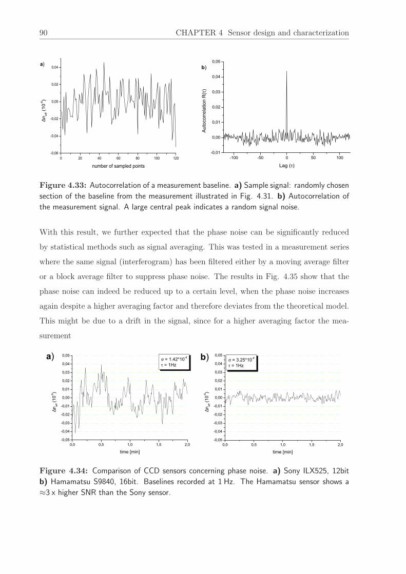
90 CHAPTER 4 Sensor design and characterization
-100 -50 0 50 100-0,01
0,00
0,01
0,02
0,03
0,04
0,05b)
Auto
corre
latio
n R
(τ)
Lag (τ)0 20 40 60 80 100 120
-0,06
-0,04
-0,02
0,00
0,02
0,04a)
∆n ef
f (10
-6)
number of sampled points
Figure 4.33: Autocorrelation of a measurement baseline. a) Sample signal: randomly chosen
section of the baseline from the measurement illustrated in Fig. 4.31. b) Autocorrelation of
the measurement signal. A large central peak indicates a random signal noise.
With this result, we further expected that the phase noise can be significantly reduced
by statistical methods such as signal averaging. This was tested in a measurement series
where the same signal (interferogram) has been filtered either by a moving average filter
or a block average filter to suppress phase noise. The results in Fig. 4.35 show that the
phase noise can indeed be reduced up to a certain level, when the phase noise increases
again despite a higher averaging factor and therefore deviates from the theoretical model.
This might be due to a drift in the signal, since for a higher averaging factor the mea-
surement
b)a)
0,0 0,5 1,0 1,5 2,0-0,05
-0,04
-0,03
-0,02
-0,01
0,00
0,01
0,02
0,03
0,04
0,05σ = 1.42*10-8
τ = 1Hz
∆nef
f (10
-6)
time [min]0,0 0,5 1,0 1,5 2,0
-0,05
-0,04
-0,03
-0,02
-0,01
0,00
0,01
0,02
0,03
0,04
0,05σ = 3.25*10-9
τ = 1Hz
∆nef
f (10
-6)
time [min]
Figure 4.34: Comparison of CCD sensors concerning phase noise. a) Sony ILX525, 12bit
b) Hamamatsu S9840, 16bit. Baselines recorded at 1 Hz. The Hamamatsu sensor shows a
≈3 x higher SNR than the Sony sensor.

4.2 Interferometric biosensor: flow cell system 91
time has to be increased to reach a statistically significant amount of sampled values,
i.e. in this case long-term effects in the signal show up. Yet the good agreement with the
0 10 20 30 40 50 60 70 80 90 100 110 1200,000
0,005
0,010
0,015
0,020
0,025
0,030b)
Model: Y=1/(A+B*sqrt(X)) A 17.67 ±4.33B 18.93 ±3.01
R2 0.56668
sd n
eff (
10-6)
averaging factor n0 20 40 60 80 100 120
0,000
0,005
0,010
0,015
0,020
0,025
0,030a)
Model: Y=1/(A+B*sqrt(X))
A 15.64 ±5.15B 23.14 ±3.73
R2 0.8762
sd n
eff (
10-6)
averaging factor n
Figure 4.35: Phase noise reduction by signal averaging. a) Application of a moving av-
erage filter b) Application of a block average filter. Measurement parameters: R=12.5 kΩ,
I=115 mA, τ=400 ms.
fit model for averaging factors up to 16-32 support the theoretical correlation between
phase noise reduction and averaging factor described in the previous section. Apart from
the statistical structure of the baseline noise non-random effects can occur: an example
of a signal distortion arising due to program conflicts with the Windows operating system
is shown in Fig. 4.36.
0 50 100 150 200
500
1000
1500
2000
2500
mea
n [in
tens
ity]
time [sec]
Figure 4.36: Non-random signal distortion in the CCD readout due to a program conflict
with the Windows operating system.

92 CHAPTER 4 Sensor design and characterization
These distortions occur mainly at short exposure times below 50 ms and are characterized
by an over-saturation of the CCD pixels caused by a delayed readout of the CCD camera.
To avoid these distortions during a running experiment, it is recommended to only run
the interferometer software and work at exposure times above 50 ms. Furthermore phase
fluctuations due to light source instability combined with path length differences in the
setup can severely distort the signal as illustrated in Fig. 4.37. Fox et al. (1999) estimated
an uncertainty in wavelength of a Helium-Neon laser to∆λDoppler
λ= 3.2 · 10−6 caused by
the Doppler width of the Ne emission line. Assuming a misalignment of the two beam
paths of only 200 µm, this results in a fluctuation on the order of 1 · 10−7, representing a
major disturbance in the signal. Yet the short-term noise in ∆neff remains on the order of
3 · 10−8, the same value as it has been found with the SLD as light source. Based on these
findings the SLD was chosen as main light source due to its better wavelength stability.
0 10 20 30 40 50 6055,0
55,5
56,0
56,5
57,0
57,5
58,0
58,5
59,0
∆nef
f (10
-6)
time [min]
σ=3.862*10-8
σ=3.29*10-8
Figure 4.37: Influence of light source instability on signal noise. Measurement recorded
with a Helium-Neon laser at λ = 632.8nm. Severe fluctuations in the signal can be observed,
which are mainly due to wavelength fluctuations from the laser combined with path length
differences in the optical setup.
4.2 Interferometric biosensor: flow cell system 93
4.2.6 Conclusion
This chapter describes the realized setup of the interferometric biosensor with a flow cell
as fluidic element, discussing all system components and their characterization in detail.
From the analysis of system components a number of conclusions can be made, such as the
choice of materials for the waveguide chips, the light source and the CCD detector. The
characteristics of the chosen components influence the final design and setup, leading to
an optimal set of parameters for the interferometric biosensor. Further a detailed system
characterization by refractometric test measurements is provided including an evaluation
of the experimental results compared to theoretical calculations and simulations.
Initial refractometric test measurements with glycerin have shown an effective refractive
index resolution of ∆neff ≈ 6.0 · 10−8, corresponding to a refractive index resolution of
∆n ≈ 7.5 · 10−7 for TE mode and ∆n ≈ 2.7 · 10−7 for TM mode, respectively, at a sam-
pling rate of 1 Hz. This resolution has been improved by a factor of 3 by implementing
a new CCD sensor with full-line binning on the CCD chip. It was also found that the
CCD sensor is the limiting system component concerning noise, whereas the phase noise
is approximately equal for all three light sources tested and therefore the light source
can be excluded as limiting factor. Signal filtering methods such as averaging have been
implemented and analyzed concerning their suitability for phase noise reduction.
The experimentally derived sensitivity constants of the interferometer system are in very
good accordance with the theoretical values derived from waveguide theory. The system
shows a good long-term stability with a typical drift of < 1 · 10−6/h in ∆neff .

94 CHAPTER 4 Sensor design and characterization
4.3 Interferometric biosensor: microplate system
4.3.1 Introduction
The use of microtiterplates (MTP) has become a standard for laboratory routine screening
tests (e.g. enzyme-linked immunosorbent assays (ELISA)), where a high sample through-
put is required (Blake, 2001). MTP’s are commonly configured as 96-, 384- or 1536-well
plates in a standard format of 127.8 mm x 85.6 mm, compatible with the majority of com-
mercially available readout systems. In general, the assay of interest is performed before
inserting the MTP into the readout system. Yet a direct monitoring of the assay perfor-
mance including intermediate steps could be of great advantage. This section describes
the development of the interferometric biosensor implementing an MTP-formatted frame
(IBS 801). This combination of a standard MTP format with label-free detection allows
the direct readout of assay results.
A main part of the work has been devoted to the development of a prototype setup with
an 8-well microplate (see Fig. 4.38). The microplate is formatted as a section of a 96-well
MTP. First refractometric test measurements and a biological test measurement will be
presented in chapter 5. The system design allows an extension to read plates in the com-
monly known 96- or 384 well MTP formats.
Figure 4.38: Reader options. a) Flow cell system, 2 channel b) Microplate system, 8-well
configuration
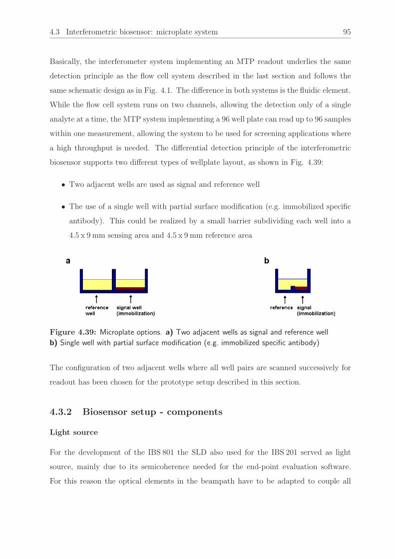
4.3 Interferometric biosensor: microplate system 95
Basically, the interferometer system implementing an MTP readout underlies the same
detection principle as the flow cell system described in the last section and follows the
same schematic design as in Fig. 4.1. The difference in both systems is the fluidic element.
While the flow cell system runs on two channels, allowing the detection only of a single
analyte at a time, the MTP system implementing a 96 well plate can read up to 96 samples
within one measurement, allowing the system to be used for screening applications where
a high throughput is needed. The differential detection principle of the interferometric
biosensor supports two different types of wellplate layout, as shown in Fig. 4.39:
• Two adjacent wells are used as signal and reference well
• The use of a single well with partial surface modification (e.g. immobilized specific
antibody). This could be realized by a small barrier subdividing each well into a
4.5 x 9 mm sensing area and 4.5 x 9 mm reference area
Figure 4.39: Microplate options. a) Two adjacent wells as signal and reference well
b) Single well with partial surface modification (e.g. immobilized specific antibody)
The configuration of two adjacent wells where all well pairs are scanned successively for
readout has been chosen for the prototype setup described in this section.
4.3.2 Biosensor setup - components
Light source
For the development of the IBS 801 the SLD also used for the IBS 201 served as light
source, mainly due to its semicoherence needed for the end-point evaluation software.
For this reason the optical elements in the beampath have to be adapted to couple all

96 CHAPTER 4 Sensor design and characterization
spectral contributions into the waveguide chip and focus them onto the CCD camera to
achieve a narrow interference area. The laser diode described in chapter 4.2.1 also emits
semicoherent light below threshold, yet the available power is too low to operate the
system in TM mode.
Optical elements and double slit
The optical elements that have been integrated into the system are similar to the ones used
for the flow cell system (see also Fig. 4.42). The divergent beam emitted by the SLD is
collimated by an apherical lens with a focal length of f1 = 8 mm and focused as a line onto
the chip grating by a cylindrical lens with f2 = 100 mm. Focusing on the grating ensures
in this case the coupling of all spectral contributions into the waveguide and further to
couple a high light intensity. In contrast to the setup of the flow cell system, yet another
cylindrical lens is needed in the beampath between the double slits and the CCD detector
to focus again all spectral contributions. As illustrated in Fig. 4.42, each wavelength is
coupled out at a different angle, and the cylindrical lens focuses the divergent beam onto
the CCD camera so that the complete spectrum is detected. Again all lenses were ordered
from Thorlabs, USA and are made of BK7 glass with a refractive index of 1.52, carrying
an antireflection coating.
The double slit plate used has the same design and dimensions as described in chapter
4.2.1, except that the slit distance has been changed to 2 mm to adapt the distance of the
two beams to the dimensions of the microplate frame.
Optics mount
The optics mount for the IBS 801 is a special design and fabricated at the IPM. It essen-
tially comprises two adjustable mirrors (≈3 mm x 7 mm) that redirect the beam almost
orthogonally, as illustrated in Fig. 4.40. By two screws placed in front the mirrors can be
adjusted for incoupling, or directing the outcoupled beam centrically through the cylin-
drical lens onto the CCD camera. The optics mount provides a small cutout on top for
the double slit plate.

4.3 Interferometric biosensor: microplate system 97
Figure 4.40: Design of the IBS 801 optics mount (CAD drawing). Two mirrors for in- and
outcoupling can be adjusted by screws. The double slit plate is placed on top.
Waveguide chips and CCD camera
The same waveguide chips as for the IBS 201 supplied by Unaxis Optics have been used
for the IBS 801 prototype setup. For a 96-well MTP a complete wafer of accordant size
would be implemented.
The CCD device mainly used during the system development is the CCD1000 described
in chapter 4.2.1 with the ILX 526A line sensor.
Microplate frames
An MTP-formatted 8-well frame represents the fluidic element of the IBS 801. It is made
of the chemically inert thermoplastic PEEK™ and has been specially designed at the IPM
for use with the available waveguide chip format provided by Unaxis. Basically it can be
classified as section of a bottomless 96-well MTP as commercially available. A schematic
drawing of the 8-well frame attached to a waveguide chip is shown in Fig. 4.41. The
four gratings lie directly below the bars of the MTP frame, and each pair of adjacent
wells serves as measurement and reference well. A step motor moves the MTP frame
successively to the next well pair; hence four parallel measurements can be performed by
scanning the plate. A specially designed frame holder mounted on the step motor keeps
the waveguide chip including the MTP frame ≈1 mm above the optics mount and the
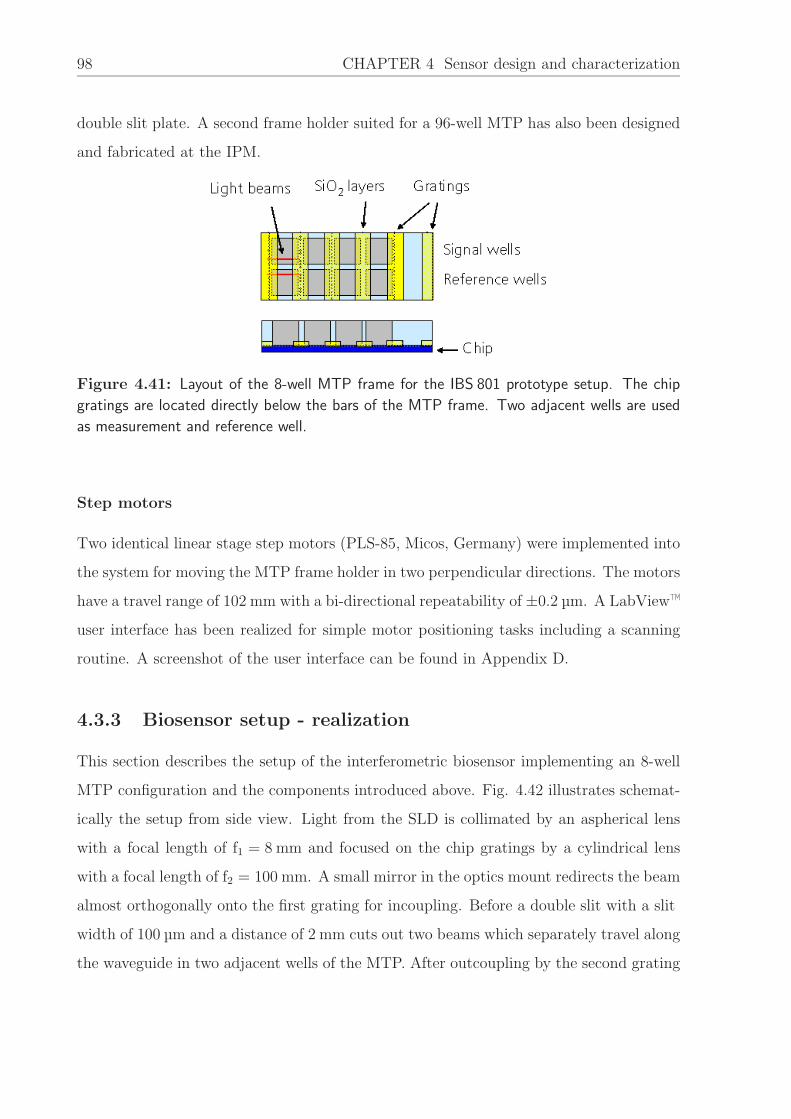
98 CHAPTER 4 Sensor design and characterization
double slit plate. A second frame holder suited for a 96-well MTP has also been designed
and fabricated at the IPM.
Figure 4.41: Layout of the 8-well MTP frame for the IBS 801 prototype setup. The chip
gratings are located directly below the bars of the MTP frame. Two adjacent wells are used
as measurement and reference well.
Step motors
Two identical linear stage step motors (PLS-85, Micos, Germany) were implemented into
the system for moving the MTP frame holder in two perpendicular directions. The motors
have a travel range of 102 mm with a bi-directional repeatability of ±0.2 µm. A LabView™
user interface has been realized for simple motor positioning tasks including a scanning
routine. A screenshot of the user interface can be found in Appendix D.
4.3.3 Biosensor setup - realization
This section describes the setup of the interferometric biosensor implementing an 8-well
MTP configuration and the components introduced above. Fig. 4.42 illustrates schemat-
ically the setup from side view. Light from the SLD is collimated by an aspherical lens
with a focal length of f1 = 8 mm and focused on the chip gratings by a cylindrical lens
with a focal length of f2 = 100 mm. A small mirror in the optics mount redirects the beam
almost orthogonally onto the first grating for incoupling. Before a double slit with a slit
width of 100 µm and a distance of 2 mm cuts out two beams which separately travel along
the waveguide in two adjacent wells of the MTP. After outcoupling by the second grating

4.3 Interferometric biosensor: microplate system 99
Figure 4.42: Schematic drawing of the IBS 801 setup - side view. An aspheric lens collimates
the divergent beam emitted by the SLD, followed by a cylindrical lens to focus a line on the
grating. After passing the waveguide chip in two separate beams, the outcoupled, divergent
beam is refocused on the CCD camera to ensure all spectral contributions are maintained in
the interferogram.
the beams pass again a double slit with a slit width of 3 µm or 5 µm and the resulting
interferogram is finally, refocused by a second cylindrical lens, recorded by the CCD cam-
era. Fig. 4.43 displays a schematic drawing of the setup in top view. Special attention
Figure 4.43: Schematic drawing of the IBS 801 setup - top view.
has been paid to choose the suitable focal lengths of the cylindrical lenses, since they
represent the crucial elements for coupling the complete spectral bandwidth of the SLD.
A focal length of 100 mm to focus on the incoupling grating seemed appropriate to couple
the total spectral bandwidth of the SLD, as calculated and discussed in chapter 4.2.3.

100 CHAPTER 4 Sensor design and characterization
Figure 4.44: Simulation of the beampath from the outcoupling grating (left) to the CCD
sensor (right) with Optalix™. The optimal position for the cylindrical lens has been determined
to 43 mm from the CCD sensor.
A simulation program for calculating optical lenses and their foci (Optalix™) has been
used to model the beampath extending from the outcoupling grating to the CCD sensor.
Resulting from this simulation the optimal position for the CCD sensor is at a distance of
120 mm from the outcoupling grating, with the rear surface of the cylindrical lens located
at a distance of 43 mm from the CCD sensor. Fig. 4.44 illustrates the beampath starting
at the outcoupling grating (left) to the CCD sensor (right). Fig. 4.45 presents the current
prototype setup of the IBS 801 used for the measurements described in the next section
and in chapter 5.
Figure 4.45: Top view photograph of the interferometric biosensor IBS 801. Refer to Fig.
4.42 for details on the optical components.
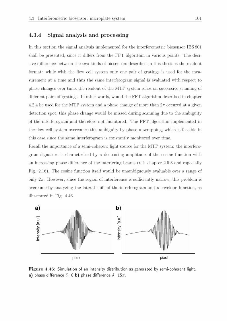
4.3 Interferometric biosensor: microplate system 101
4.3.4 Signal analysis and processing
In this section the signal analysis implemented for the interferometric biosensor IBS 801
shall be presented, since it differs from the FFT algorithm in various points. The deci-
sive difference between the two kinds of biosensors described in this thesis is the readout
format: while with the flow cell system only one pair of gratings is used for the mea-
surement at a time and thus the same interferogram signal is evaluated with respect to
phase changes over time, the readout of the MTP system relies on successive scanning of
different pairs of gratings. In other words, would the FFT algorithm described in chapter
4.2.4 be used for the MTP system and a phase change of more than 2π occured at a given
detection spot, this phase change would be missed during scanning due to the ambiguity
of the interferogram and therefore not monitored. The FFT algorithm implemented in
the flow cell system overcomes this ambiguity by phase unwrapping, which is feasible in
this case since the same interferogram is constantly monitored over time.
Recall the importance of a semi-coherent light source for the MTP system: the interfero-
gram signature is characterized by a decreasing amplitude of the cosine function with
an increasing phase difference of the interfering beams (ref. chapter 2.5.3 and especially
Fig. 2.16). The cosine function itself would be unambiguously evaluable over a range of
only 2π. However, since the region of interference is sufficiently narrow, this problem is
overcome by analyzing the lateral shift of the interferogram on its envelope function, as
illustrated in Fig. 4.46.
b)a)
inte
nsity
[a.u
.]
inte
nsity
[a.u
.]
pixel pixel
Figure 4.46: Simulation of an intensity distribution as generated by semi-coherent light.
a) phase difference δ=0 b) phase difference δ=15π.

102 CHAPTER 4 Sensor design and characterization
The maximum of the envelope function determines the interference order so that an un-
ambiguous evaluation, i.e. a so-called end-point evaluation, of the interferogram signal
is achieved (Brandenburg , 1997). The implemented algorithm basically consists of two
steps: first, the maximum of the envelope function is determined by evaluating the cross-
correlation of a reference distribution with the sampled interferogram signal. In a second
step the phase of the respective interference order is calculated. Once the spatial period
of the interferogram has been determined by an FFT, two reference distributions si and
ci with the same spatial resolution are calculated by the algorithm according to:
si =
sin(2πip
)[1 + cos(2πib
)] for − b2≤ i ≤ b
2
0 for i > b2
and i < −b2
(4.7)
and
ci =
cos(2πip
)[1 + cos(2πib
)] for − b2≤ i ≤ b
2
0 for i > b2
and i < −b2
(4.8)
with b being the width of the envelope function and p the period; i denotes an integer
number corresponding to the pixels of the CCD camera. Fig. 4.47 shows examples of
such reference distributions with b=50 and p=5.8.
0 10 20 30 40 50-2,0
-1,5
-1,0
-0,5
0,0
0,5
1,0
1,5
2,0b)
inte
nsity
pixel0 10 20 30 40 50
-2,0
-1,5
-1,0
-0,5
0,0
0,5
1,0
1,5
2,0a)
inte
nsity
pixel
Figure 4.47: Calculated sine and cosine reference distributions for cross-correlation with the
interferogram signal a) Sine function b) Cosine function

4.3 Interferometric biosensor: microplate system 103
Once the reference distributions are determined, the interferogram signal is cross-correlated
with the reference distributions according to:
Sk =∑
xisi−k (4.9)
Ck =∑
xici−k (4.10)
where k denotes the pixel number for all pixel values from 0 to 2048 (or 3000). Fig.
4.48 displays this cross-correlation graphically. The maximum of the cross-correlation
function, indicating the interference order, is given by:
T = S2k + C2
k (4.11)
Figure 4.48: Intensity distribution resulting from the cross-correlation of an interferogram
signal with its respective reference distributions. The maximum of this distribution determines
the maximum of the interferogram’s envelope function and thus the interference order.
After the interference order has been found, the phase of the interferogram can be calcu-
lated by using the similar reference distributions, but with envelope widths b correspond-
ing approximately to the envelope width of the original signal and taking the coefficients:
S0 =∑
xisi (4.12)
C0 =∑
xici (4.13)
The corresponding phase is given by:
φ = −arctanS0
C0
(4.14)

104 CHAPTER 4 Sensor design and characterization
For the calculation of the effective refractive index and the refractive index the same
formula apply as for the FFT algorithm. A flowchart of the complete cross-correlation
algorithm can be found in Appendix D.
The same signal filtering methods (zeropadding, average filters) have been added to the
algorithm for signal refining and noise reduction. The effects of these filters within the
cross-correlation algorithm correspond to the results shown with the FFT algorithm and
will therefore not be discussed further in this section.
4.3.5 Simulation algorithm for signal analysis
Based on the two signal evaluation algorithms described before, a separate routine for
interferogram simulation has been developed in order to test newly implemented routines.
Interferogram parameters characterizing the envelope function and the coherence function
can be chosen, as well as the addition of random pixel noise to the signal. This test
function has been implemented into the Labview™ interface instead of the CCD readout
routine and undergoes the same FFT and cross-correlation, or filtering routines, as an
original signal. A snapshot of the user interface can be found in Appendix D along with
the DLL routine of the test function.
4.3.6 Experimental characterization of the biosensor system
The experimental characterization of the relevant system components has already been
described in section 4.2.3. Here only a characterization of the biosensor system imple-
menting these components shall be given and compared to the results obtained with the
flow cell system.
Refractive index measurement
A refractometric test measurement has been performed as a preliminary test of the system
and for calibration. Here ethanol has been chosen as sample to prepare solutions of differ-
ent refractive indices due to its neutrality and fast dissolving in H2O. All measurements
were performed as follows:

4.3 Interferometric biosensor: microplate system 105
• Preparation of a stock solution of 1% (v/v) ethanol in DI − H2O
• Preparation of dilutions from the stock solution in the range of 0.2% to 1% in a
total volume of 100 µl in separate reaction vessels; the concentrations need to be
twice as high as the desired concentration for measurement
• The interferometer system is prepared by inserting the MTP-chip, checking for
incoupling (i.e. interferogram) at each well pair and filling all 8 wells with 100 µl
DI − H2O
• All system parameters like exposure time, SLD current and averaging factors should
be reasonably set and adjusted. Ideally the intensity of the detected interferogram
signal is similar for all well pairs
Figure 4.49: Layout of the 8-well MTP chip
Before the measurement is started, all four well pairs need to be scanned and the signal
drift observed (H2O-baseline). Once the drift falls below 5 · 10−6 in ∆neff , the measure-
ment can be started by pipetting 100 µl of each ethanol solution in well B1-B4, keeping
A1-A4 as reference (see Fig. 4.49). Since ethanol dissolves very quickly in H2O, scanning
of the well pairs can be resumed and the respective values for ∆neff determined. Typically
each well pair is scanned for a time interval of 10 sec in 8-10 repetitive measurements.
Fig. 4.50 presents the results of a test measurement with ethanol concentrations ranging
from 0.1% to 0.5% (v/v).
Fig. 4.51 shows the calibration curve corresponding to this measurement, where the mean
signal change in ∆neff for each concentration is plotted versus the refractive index ob-
tained from literature (Weast , 1976). Values below 0.5% are estimated by a polynomial

106 CHAPTER 4 Sensor design and characterization
0,0 0,1 0,2 0,3 0,4 0,5 0,60
2
4
6
8
10
12
14
16
∆nef
f(*10
-6)
concentration in % (v/v)
Figure 4.50: Refractive index measurement with ethanol solutions from 0.1% to 0.5% (v/v)
as sample. Measurement parameters: SLD TE, R=12.5 kΩ, I=55 mA, τ=200 ms. Error bars
denote the standard deviation from the mean of eight repeated measurements.
0,00010 0,00015 0,00020 0,00025 0,00030 0,00035
0,000000
0,000002
0,000004
0,000006
0,000008
0,000010
0,000012
0,000014
0,000016
Linear Regression Y=A+B*X
A -6,71*10-6 5,99*10-7
B 0,067 0,0025
R2 0,99713
∆nef
f
∆n0
Figure 4.51: Calibration curve derived from ethanol concentration measurements for TE
mode. The mean signal change in ∆neff for each concentration is plotted versus the refractive
index n. From the slope of the linear fit the sensitivity constant can be determined to∆neff
∆n0=
0.067.
fit (cf App. C). The data were then fitted to a linear regression model to determine the
sensitivity constant. Yielding an experimental value of∆neff
∆n0= 0.067 compared to the
theoretical value of∆neff
∆n0= 0.082, it can be seen that the measurement is diffusion limited.

4.3 Interferometric biosensor: microplate system 107
Comparison with flow cell system
In order to compare the characteristics of the microplate system with the flow cell system,
the same test measurement with ethanol concentrations has also been performed with the
flow cell system. All preparations were in accordance with the description given in chapter
4.2.5. Fig. 4.52 illustrates the results obtained from both systems.
0,0 0,1 0,2 0,3 0,4 0,5
0
2
4
6
8
10
12
14
16 IBS 201 (flow cell) IBS 801 (MTP)
∆nef
f (10
-6)
concentration in % (v/v)
Figure 4.52: Comparison of refractive index measurements with ethanol concentrations
ranging from 0.1% to 0.5% (v/v), performed on both bionsensor systems. The signal values
in ∆neff are systematically lower in the microplate system.
It can be observed that the ∆neff values obtained with the microplate system are sys-
tematically lower than the values obtained with the flow cell system, as already seen in
Fig. 4.50. This might be due to a limited diffusion in the MTP wells, whereas the sample
solution is brought directly in contact with the waveguide surface in the flow cell.
Characterization of signal noise and repeatability
Equivalent to the flow cell system, the characterization of the MTP system included the
determination of signal drift and noise. Additionally, the repeatability, i.e. the variation
of measurement values influenced by scanning, has to be considered. The repeatability
mainly depends on the bi-directional repeatability of the step motors, and possible mis-

108 CHAPTER 4 Sensor design and characterization
alignments of the optical components including the waveguide chip. As a first test, a
waveguide chip without liquid samples has been scanned for 8 data values as illustrated
in Fig. 4.53. The standard deviation of the mean yields the information about the re-
peatability, which was found to be on the order of 1 · 10−7 in ∆neff for all well pairs.
1 2 3 4 5 6 7 8
-4
-3
-2
-1
0
1
A1/B1 sd=0.9*10-7
A2/B2 sd=1.5*10-7
A3/B3 sd=1.5*10-7
A4/B4 sd=1.6*10-7
∆nef
f(10-6
)
scan #
Figure 4.53: Repeatability characteristics of the microplate system. The standard deviation
of the mean of eight recorded ∆neff values determines the repeatability of the measurement
data.
0 5 10 15 20-24
-22
-20
-18
-16
-14
-12
-10
-8σ=1.5*10-8 (1Hz)drift: 4.5*10-5/h
∆nef
f (10
-6)
time [min]
Figure 4.54: Baseline recorded with the microplate system showing a drift of 4.5 · 10−5/h
in ∆neff . Parameters: R=12.5 kΩ, I=120 mA, τ=1000 ms

4.3 Interferometric biosensor: microplate system 109
To characterize the signal noise and drift over time, a simple baseline measurement was
performed and is presented in Fig. 4.54. While the signal noise is equal to the signal
noise of the flow cell system, a larger signal drift can be observed, being typically around
5 · 10−5/h in ∆neff . This estimation is however only valid provided that the MTP chip has
been inserted into the system about half an hour before the measurement. With newly
inserted chips, the system shows an increased drift. To avoid disturbances of the measure-
ment data due to a large drift, the chip should be inserted and not moved again about
half an hour previous to measurements. To compensate the influence of signal drifts in
application measurements, one well pair (typically A1/B1) should always be kept under
buffer conditions and the drift thereof determined. This allows a baseline correction and
thus drift compensation for the other measurement data.
4.3.7 Conclusion
This chapter describes the realized setup of the interferometric biosensor with an MTP-
formatted 8-well frame as fluidic element and discussing newly introduced system com-
ponents that are different from the flow cell system. Again, the choice of suitable system
components influences the design and setup of the interferometer system with an opti-
mal set of parameters. Further a detailed system characterization by refractometric test
measurements is provided including an evaluation of the experimental results compared
to theory and the results obtained with the flow cell system.
Initial refractometric test measurements with ethanol have shown an effective refractive in-
dex resolution of ≈ 1.0 · 10−7, corresponding to a refractive index resolution of ≈ 1.2 · 10−6
for TE mode and ≈ 4.5 · 10−7 for TM mode, respectively, at a sampling rate of 1 Hz. It
was also found that, apart from the CCD sensor being the limiting system component
concerning noise, the resolution of the system is finally limited by the repeatability of the
recorded data values. The experimentally derived sensitivity constants of the microplate
interferometer system are also in good accordance with the theoretical values derived from
waveguide theory (82%). The system shows a long-term stability with a typical drift of
< 5 · 10−5/h in ∆neff and a repeatability of < 2 · 10−7 in ∆neff .


Chapter 5
Application measurements
5.1 Introduction
This chapter presents the materials and methods used for the application measurements
as well as a detailed description and characterization of the surface chemistry for the
functionalization of the waveguide sensor chips. The interferometric biosensor is used
to monitor different immunoreactions and their binding kinetics are evaluated and dis-
cussed. A streptavidin-functionalized surface is compared with fluorescent detection to
characterize the surface chemistry.
5.2 Materials and methods
5.2.1 Materials
Chemicals and biochemicals
A complete list of all chemicals and their vendors can be found in Appendix A.
The following buffers and regeneration solutions were used for the experiments:
• PBS: Phosphate buffered saline; running buffer prepared from PBS concentrate
1 : 10 diluted with DI − H2O. Isoosmotic buffered saline to provide a stable en-
vironment for biological substances with a pH of ≈7.4 at a temperature of 25 C.
111

112 CHAPTER 5 Application measurements
To prevent analyte molcules from attaching to vial or tubing walls or denaturing in
pure PBS, BSA in concentrations from 0.1% to 1% (w/v) can be added
• NaOH, 50-100 mM: alkaline regeneration solution
• HCl, 50-100 mM: acidic regeneration solution
• H3PO4, 10-100 mM: acidic regeneration buffer, adjusted to pH=2 with NaOH
• Analyte buffer: Cleaned cell lysate from Escherichia coli
• Washing buffer: Mix 100 ml SSC (20x concentrate) with 10 ml SDS and 0.5 ml
Tween 20 and fill with DI − H2O to a total volume of 1000 ml
Devices and transducers
Apart from the IBS 201 and IBS 801 setup and their components described in chapter 4,
following devices have been used for the experiments:
• SPR devices: BIACORE 1000 Upgrade and BIACORE 2000, BIACORE AB, Upp-
sala, Sweden
• Sensorchip for BIACORE: Sensor Chip SA (Streptavidin-coated dextran matrix)
• Fluorescence reader: BCR 101 laser reader, Fraunhofer IPM Freiburg
• pH-meter: MP 225, Mettler Toledo, Giessen, Germany
• Powermeter: Newport Model 1830C, detector 818-IR
• Optical spectrum analyzer: Ando, AQ 6315A-B
• Microarray printer: Genetix QArraymini
• Micro balance: Sartorius CP225D
All data are evaluated and represented with Microcal Origin© (versions 5.0 and 6.1).
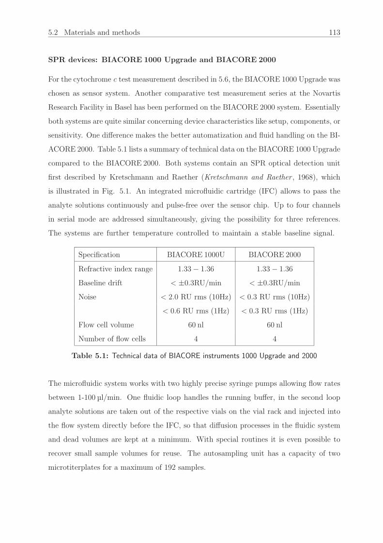
5.2 Materials and methods 113
SPR devices: BIACORE 1000 Upgrade and BIACORE 2000
For the cytochrome c test measurement described in 5.6, the BIACORE 1000 Upgrade was
chosen as sensor system. Another comparative test measurement series at the Novartis
Research Facility in Basel has been performed on the BIACORE 2000 system. Essentially
both systems are quite similar concerning device characteristics like setup, components, or
sensitivity. One difference makes the better automatization and fluid handling on the BI-
ACORE 2000. Table 5.1 lists a summary of technical data on the BIACORE 1000 Upgrade
compared to the BIACORE 2000. Both systems contain an SPR optical detection unit
first described by Kretschmann and Raether (Kretschmann and Raether , 1968), which
is illustrated in Fig. 5.1. An integrated microfluidic cartridge (IFC) allows to pass the
analyte solutions continuously and pulse-free over the sensor chip. Up to four channels
in serial mode are addressed simultaneously, giving the possibility for three references.
The systems are further temperature controlled to maintain a stable baseline signal.
Specification BIACORE 1000U BIACORE 2000
Refractive index range 1.33 − 1.36 1.33 − 1.36
Baseline drift < ±0.3RU/min < ±0.3RU/min
Noise < 2.0 RU rms (10Hz) < 0.3 RU rms (10Hz)
< 0.6 RU rms (1Hz) < 0.3 RU rms (1Hz)
Flow cell volume 60 nl 60 nl
Number of flow cells 4 4
Table 5.1: Technical data of BIACORE instruments 1000 Upgrade and 2000
The microfluidic system works with two highly precise syringe pumps allowing flow rates
between 1-100 µl/min. One fluidic loop handles the running buffer, in the second loop
analyte solutions are taken out of the respective vials on the vial rack and injected into
the flow system directly before the IFC, so that diffusion processes in the fluidic system
and dead volumes are kept at a minimum. With special routines it is even possible to
recover small sample volumes for reuse. The autosampling unit has a capacity of two
microtiterplates for a maximum of 192 samples.

114 CHAPTER 5 Application measurements
Figure 5.1: SPR setup based on Kretschmann and Raether. Depending on the refractive
index in the evanescent field above the gold layer, the angle of the reflected light changes. This
variation is seen as a dip in the intensity distribution and can be very sensitively monitored as
resonance signal. The signal intensity is given in resonance units (R.U.). One resonance unit
corresponds to a surface coverage of 1pg/mm2. Adapted from www.biacore.com (2003).
A customized software controls all steps of the measurement routine and performs the
evaluation of the binding curves for obtaining binding constants and surface coverages.
In-line referencing is done by subtracting the binding curves from different flow cell chan-
nels. Furthermore, readily immobilized chips with a variety of surface chemistries for
different assay applications are available (van der Merwe, 2005).
Biochip Reader BCR 101
For all experiments with labeled molecules the biochip reader BCR 101 was used for fluo-
rescence imaging. The system comprises a Helium-Neon laser (633 nm) for the excitation
of the fluorescent dyes and allows wavelength-selective imaging at (680±15)nm. The im-
ages are recorded by a cooled CCD camera (Apogee, USA) with an array of 765 x 512
pixels. The 16 bit information (intensity) can be illustrated in false color. A customized
software controls the exposure time and the CCD parameters. Optional routines include
dark current correction and illumination correction of the recorded image. All images in
experiments described below are dark current corrected.

5.2 Materials and methods 115
5.2.2 Methods
Cleaning of waveguide chips
The waveguide chips have to be cleaned thoroughly before silanization or measurements
according to the degree of possible previous contamination and usage. Generally, using a
new chip for each measurement is advisable, but not necessary since they can be regen-
erated to an acceptable level after silanization and reused. Table 5.2 gives an overview of
cleaning procedures that have proven to be suitable and do not cause any damage to the
waveguide and protective layers (see also 5.2.1).
Degree of contamination/usage Cleaning procedure
new 10 min in isopropanol in ultrasonic bath,
for refractometric test measurement rinsing with DI − H2O, drying
or: 30 min in 0.5 % (v/v) Hellmanex solution
(using more than 0.5 % causes the SiO2
protective layers to come off)
new, for silanization 30min at 75 C in 3:1 25% NH3 : 30% H2O2,
rinsing with DI − H2O, drying
used, not silanized 15sec in 10M NaOH, rinsing with DI − H2O,
10 min in isopropanol in ultrasonic bath,
rinsing with DI − H2O, drying
used, silanized up to 40sec in 10M NaOH, rinsing with DI − H2O,
(complete regeneration) 30 min at 75 C in 3:1 25% NH3 : 30% H2O2,
rinsing with DI − H2O, drying
Table 5.2: Cleaning procedures for waveguide chips
Silanization
The treatment with 3:1 25% NH3 : 30% H2O2 previous to silanization turns the chip sur-
face highly hydrophilic (caused by OH−-groups). Each hydroxyl group should ideally
capture one silane molecule, resulting in a silane monolayer, and the amount of silane

116 CHAPTER 5 Application measurements
molecules on the surface increases with the degree of hydroxyl groups (Le Grange and
Markham, 1993). A high density of silanes on the surface ensures a stable and repro-
ducible surface modification and reduces unspecific binding to a minimum. The silaniza-
tion for all experiments described has been done at the IPM in a special silanization
device for working under an argon atmosphere. Argon acts in this case as cover gas to
prevent the reagents from coming into contact with humidity. Even a very small water
content in the silane solvents would cause the silane molecules to polymerize, resulting in
an unordered, multi-layered silane surface not suitable for reproducible measurements. A
schematic drawing of the silanization device is shown in Fig 5.2.
Figure 5.2: Silanization device. Chips and silanization reagents are handled in glass reaction
vessels. After vacuuming, the whole device is flooded with argon cover gas to protect the
silane from humidity.
The complete protocol for silanization can be found in Appendix B. After cleaning the
chips are placed in the reaction vessels. The whole device is evacuated to a pressure be-
low 1 mbar (manometer for control) and subsequently flooded with argon. The remaining
outlet can be used to keep the reagents under argon during handling. Under argon flow
10 ml toluene, 28.8 µl triethylamine and 28.8 µl (epoxy-) silane are filled into each reaction

5.2 Materials and methods 117
vessel. After a reaction time of at least 16 hours the chips are placed in a glass petri dish
and cured in an oven at 120 C for 4 hours, rinsed with DI − H2O and dried under nitro-
gen. These epoxy- (or amino-) functionalized chips can now be further modified according
to the application and assay.
Surface modification
Reaction with a spacer molecule for functionalization with amino-groups
Newly epoxy-silanized transducers are placed into pure ethylene diamine for at least 12
hours, rinsed with methanol and DI − H2O and dried. Ethylene diamine is a small spacer
molecule with a short two-carbon length that does not cause any steric problems. The
amino terminals can now be used to couple for example NHS-LC-biotin and further prepa-
ration of a streptavidin (SAv) surface. For this, a solution containing at least 1 mg/ml
NHS-LC-biotin (M = 556Da) in PBS is pipetted onto the transducer chip placed in a
humid glass chamber and incubated for at least 2 hours. After incubation the chip is
washed for 5 min in a washing buffer, rinsed with DI − H2O and dried. For subsequent
streptavidin incubation the same is done with a solution of at least 100 µg/ml SAv in
PBS. SAv-functionalized chips should be stored at 4 C until usage.
Surface characterization: contact angle measurements
One way to characterize surface properties is the measurement of a contact angle that acts
as an indicator for hydrophobicity or hydrophilicity of a (usually solid) surface. A water
drop on a solid surface represents a so-called three-phase system (Adam et al., 1995) as
shown in Fig. 5.3 with surface energies between a solid and a liquid phase (γSL), solid and
gaseous (γSV ) and liquid and gaseous (γLV ). The tangent to the drop boundary with the
solid surface gives the contact angle at equilibrium of the interfacial energies according to
Young’s equation:
γSV − γSL = γLV ∗ cosθ (5.1)
Contact angle values range from 0 on extremely hydrophilic surfaces (spreading of liquid)
up to 180 for extremely hydrophobic surfaces. Usually clean oxidic surfaces tend to be

118 CHAPTER 5 Application measurements
more hydrophilic, whereas on silanized surfaces, which are more hydrophobic, contact
angles around 60 can be measured (Elender et al., 1996; Tsukruk et al., 1999).
Figure 5.3: Contact angle θ of a liquid (water) drop on a plain solid surface. γSL, γSV and
γLV denote the surface energies between the three phases. From (Adam et al., 1995).
The contact angle can be quite easily experimentally determined. A small drop of liquid
(1 µl) on the surface of interest is imaged through a monocular telescope and monitored
by a digital camera. From the image the contact angles are quantified with the help of
an image processing software.
Fig. 5.4 shows a schematic of the setup used for our experiments. In all experiments a total
volume of 1 µl of DI − H2O was applied to the chip surface at several different positions
by a microliter syringe with a minimal dispensable volume of 0.1 µl. The water drop was
Figure 5.4: a): Setup for contact angle experiments. A water drop is placed on the surface
by a microliter syringe and monitored by a digital camera. A biconvex lens (f=40 mm) is used
for magnification. Drawing not to scale. b): typical image taken by the digital camera for
contact angle determination.
subsequently imaged through a magnifying lens by a digital camera (Aiptek MegaCam,
USA) and the contact angle on both the left and the right boundary determined by the
image processing software ImageJ© (version 1.34, open source software).

5.3 Characterization of the surface chemistry 119
Sometimes it is distinguished between an advancing contact angle which is determined
while the liquid drop is applied to the surface, and a receeding contact angle while the
liquid is taken away. Here only the equilibrium contact angle was determined.
Surface characterization: binding of fluorescently labeled streptavidin
Another issue that has to be taken into account for successful immobilization on silanized
surfaces is the total concentration of molecules that can be homogeneously bound to the
silane. Since immobilization of biotinylated reagents is a wide-spread tool for immunoas-
says, we have worked on a procedure of streptavidin coupling to the waveguide chip so
that this preparation can be used as basis for biochemical assays. In order to probe
different techniques of streptavidin immobilization and obtain information about the ho-
mogeneity and reproducibility of the functionalized surface, the binding of fluorescently
labeled streptavidin has been studied concerning these characteristics.
5.3 Characterization of the surface chemistry
5.3.1 Contact angle measurements
The contact angle measurements provide a basis for both controlling different cleaning
and regeneration methods for silanized transducers, and for characterizing the quality
and reproducibility of the silanization process. Therefore measurements were done once
directly after chip cleaning, and once after silanization with epoxysilane and modification
with ethylene diamine. Five waveguide chips with different pretreatment and history were
chosen and cleaned according to different cleaning protocols (see 5.1.2) and afterwards
placed on the setup for measuring contact angles. Since on each chip four measurement
positions on Ta2O5 are available and three subsequent pictures were taken after deposition
of the water drop, a total of 12 images giving two contact angles were evaluable. The
same applies to the SiO2-layers. The results are shown in Fig. 5.5. Fig. 5.5a depicts the
contact angles on Ta2O5 , Fig. 5.5b on the SiO2-layers. Since chip no. II was completely
new before cleaning, it served as reference for the effectiveness of the cleaning procedure.

120 CHAPTER 5 Application measurements
Chip number Pretreatment/history Cleaning procedure
I silanized, used NaOH, 25% NH3 : 30% H2O2
II new 25% NH3 : 30% H2O2
III silanized, used 25% NH3 : 30% H2O2
IV silanized, used 25% NH3 : 30% H2O2
V used for glycerol measurement 25% NH3 : 30% H2O2
Table 5.3: Pretreatment and history of waveguide chips chosen for contact angle measure-
ments and their cleaning procedures.
Chip no. I and V showed about the same contact angle on Ta2O5 as chip no. II ((55±3)).
In comparison chip no. III and IV showed a higher contact angle on Ta2O5. On SiO2, the
Figure 5.5: Contact angles on cleaned waveguide chips no. I-V as indicated in Table
5.3. a) Contact angles on the Ta2O5 surface (mean and standard deviation, N = number
of measurements). Chip no. I, II and V show lower contact angles than no. III and IV. b)
Contact angles on the protective layers (SiO2). On chip no. I and II the water drop was
spreading completely on the surface, chip no. III still showed a significant contact angle; for
chips IV and V the values are not applicable due to SiO2-layer degradation.
liquid drop spreaded on chips no. I and II, while chip no. III still showed a significant
contact angle. Due to degradation of the SiO2-layers on chips no. IV and V (might be
due to long-term storage (>1 yr) at the time of the measurement), here no values are
applicable.
The same measurements were also performed on the same chips after silanization with
GOPS, and directly after conversion of the epoxy-groups to amino terminals with ethylene
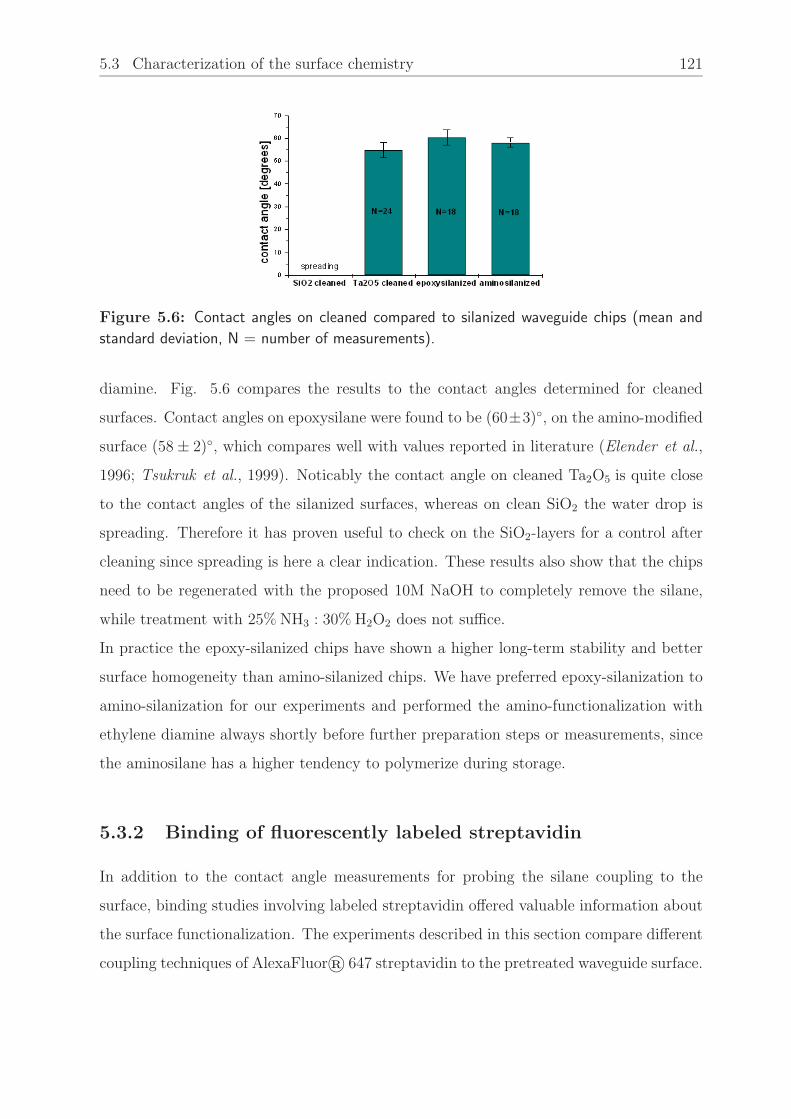
5.3 Characterization of the surface chemistry 121
Figure 5.6: Contact angles on cleaned compared to silanized waveguide chips (mean and
standard deviation, N = number of measurements).
diamine. Fig. 5.6 compares the results to the contact angles determined for cleaned
surfaces. Contact angles on epoxysilane were found to be (60±3), on the amino-modified
surface (58 ± 2), which compares well with values reported in literature (Elender et al.,
1996; Tsukruk et al., 1999). Noticably the contact angle on cleaned Ta2O5 is quite close
to the contact angles of the silanized surfaces, whereas on clean SiO2 the water drop is
spreading. Therefore it has proven useful to check on the SiO2-layers for a control after
cleaning since spreading is here a clear indication. These results also show that the chips
need to be regenerated with the proposed 10M NaOH to completely remove the silane,
while treatment with 25% NH3 : 30% H2O2 does not suffice.
In practice the epoxy-silanized chips have shown a higher long-term stability and better
surface homogeneity than amino-silanized chips. We have preferred epoxy-silanization to
amino-silanization for our experiments and performed the amino-functionalization with
ethylene diamine always shortly before further preparation steps or measurements, since
the aminosilane has a higher tendency to polymerize during storage.
5.3.2 Binding of fluorescently labeled streptavidin
In addition to the contact angle measurements for probing the silane coupling to the
surface, binding studies involving labeled streptavidin offered valuable information about
the surface functionalization. The experiments described in this section compare different
coupling techniques of AlexaFluor® 647 streptavidin to the pretreated waveguide surface.

122 CHAPTER 5 Application measurements
Fig. 5.7 provides the absorption and emission spectrum. This fluorescent dye with a
molecular weight of 1250 Da is excited at a maximum of 650 nm and shows a Stokes shift
of 18 nm, so that the maximum emission wavelength can be found at 668 nm. The labeled
streptavidin has to be stored at -20 C and needs to be prevented from absorbing daylight
to avoid bleaching of the fluorophore.
Figure 5.7: Absorption and emission spectrum of AlexaFluor® 647 and the comparable
Cy5® dye. From www.invitrogen.com (2005).
All experimental data described here were obtained with the Fluorescence Reader system
BCR 101. The spotting of the waveguide chips was performed on the Genetix QArraymini
according to the following protocol:
• Preparation of 300 µl NHS-LC-biotin solution in PBS with a concentration of 1 mg/ml
• Transfer of 60 µl biotin solution into wells A1 and B1 of a 384 MTP
• Insert the MTP and an amino-functionalized waveguide chip into the QArray
• Previous to spotting, the pin is washed with ethanol and DI − H2O and dried
• Spotting is performed at following parameters: one/two dot arrays with a dot pitch
of 560 µm on the Ta2O5 surface at a stamp time of 100 ms (contact time pin-
chip) and an ink time of 120 ms (contact time pin-sample solution); the humidity
in the device is kept at 60% during spotting; according to the manufacturer these
parameters give an approximate dot diameter of 240 µm and a dot volume of 2.3 nl
using a solid pin

5.3 Characterization of the surface chemistry 123
• After spotting the chip is transferred into a humid chamber and incubated at 4 C
for at least 2h
Following incubation, the chip is washed for 5 min in the washing buffer described in
5.1.1, rinsed with DI − H2O and dried. Subsequently the chip is incubated by pipetting
1 ml streptavidin solution (100 µg/ml SAv-AF 647 in PBS) for 1-2h, followed by the same
washing procedure. Fig. 5.8 shows an example of a biotinylated waveguide chip incubated
with labeled streptavidin.
Figure 5.8: Binding of SAv-AF 647 on biotin dots. Exposure time: 3 sec. Blue lines denote
the positions for the line scans shown in Fig. 5.9. The upper right graph shows the position
of the spotted array on the waveguide chip.
0 50 100 150 200 250 3000
10
20
30
40
50b)
inte
nsity
[a.u
.]
pixel0 50 100 150 200 250 300
0
10
20
30
40
50a)
inte
nsity
[a.u
.]
pixel
Figure 5.9: Horizontal and vertical line scans of Fig. 5.8. The results show a dot homogeneity
of >95%.

124 CHAPTER 5 Application measurements
Horizontal and vertical line scans illustrate the intensity distribution versus pixels. The
line scans can be evaluated with respect to homogeneity within a single dot, and homo-
geneity among the total number of dots on the chip. The blue lines in Fig. 5.8 denote the
positions for the line scans in Fig. 5.9 and are assumed to be representative for all dots
on the chip. The dot homogeneity was found to be very good with a standard deviation
of <5% of the mean signal value.
0 100 200 300 400 5000
20
40
60
80
100
120
140
160
180
200
220
240
260
inte
nsity
[a.u
.]
pixel
b)
a)
0 100 200 300 400 5000
50
100
150
200
250
inte
nsity
[a.u
.]
pixel
Figure 5.10: Binding of SAv-AF 647 to biotinylated surface compared to adsorption on
waveguide. a) Binding of SAv-AF 647 to biotinylated surface and the respective horizontal
linescan. Exposure time: 5 sec. b) Adsorption of SAv-AF 647 to clean waveguide chip and
the respective horizontal linescan. Exposure time: 30 sec.
The images show clearly that the biotinylated surface results in a more homogeneous binding
of SAv-AF 647 (sd<5%) than direct adsorption of SAv-AF 647 onto the waveguide surface
(sd<20%).
Further tests included the comparison of the binding/adsorption of SAv-AF 647 to dif-
ferently pretreated surfaces with the aim to find the coupling technique best suited for a
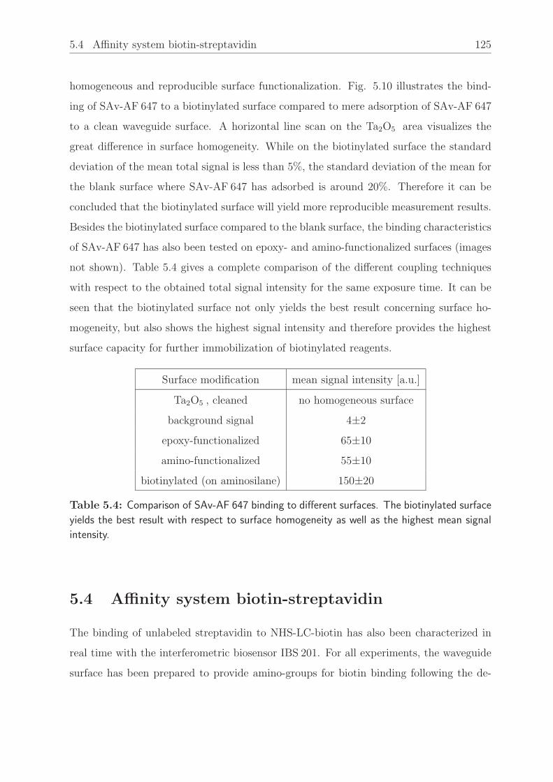
5.4 Affinity system biotin-streptavidin 125
homogeneous and reproducible surface functionalization. Fig. 5.10 illustrates the bind-
ing of SAv-AF 647 to a biotinylated surface compared to mere adsorption of SAv-AF 647
to a clean waveguide surface. A horizontal line scan on the Ta2O5 area visualizes the
great difference in surface homogeneity. While on the biotinylated surface the standard
deviation of the mean total signal is less than 5%, the standard deviation of the mean for
the blank surface where SAv-AF 647 has adsorbed is around 20%. Therefore it can be
concluded that the biotinylated surface will yield more reproducible measurement results.
Besides the biotinylated surface compared to the blank surface, the binding characteristics
of SAv-AF 647 has also been tested on epoxy- and amino-functionalized surfaces (images
not shown). Table 5.4 gives a complete comparison of the different coupling techniques
with respect to the obtained total signal intensity for the same exposure time. It can be
seen that the biotinylated surface not only yields the best result concerning surface ho-
mogeneity, but also shows the highest signal intensity and therefore provides the highest
surface capacity for further immobilization of biotinylated reagents.
Surface modification mean signal intensity [a.u.]
Ta2O5 , cleaned no homogeneous surface
background signal 4±2
epoxy-functionalized 65±10
amino-functionalized 55±10
biotinylated (on aminosilane) 150±20
Table 5.4: Comparison of SAv-AF 647 binding to different surfaces. The biotinylated surface
yields the best result with respect to surface homogeneity as well as the highest mean signal
intensity.
5.4 Affinity system biotin-streptavidin
The binding of unlabeled streptavidin to NHS-LC-biotin has also been characterized in
real time with the interferometric biosensor IBS 201. For all experiments, the waveguide
surface has been prepared to provide amino-groups for biotin binding following the de-

126 CHAPTER 5 Application measurements
scription in 5.1.2. Also recall Fig. 3.11 for the detailed binding reaction. In addition
to the surface characterizations performed with labeled streptavidin where only surface
homogeneity could be quantified, the biosensor data allows an evaluation of the binding
reaction with respect to total surface capacity and monolayer thickness.
Fig. 5.11 shows a typical sensorgram of SAv binding to immobilized biotin on an amino-
functionalized surface obtained in TE mode and at a flow rate of ≈83 µl/min. First,
a baseline under continuous PBS flow on both channels of the two-channel flow cell is
monitored for ≈10 min, followed by an injection of 1 mg/ml NHS-LC-biotin on the mea-
surement channel for ≈45 min (close to equilibrium). A washing step with PBS removes
unbound biotin, and a signal increase in ∆neff of 49 · 10−6 has been determined for the
remaining bound biotin monolayer. Following the biotin immobilization step, strepta-
vidin with a concentration of 6 µg/ml has been injected for ≈20min until equilibrium, and
washed again with PBS to remove unbound analyte. A signal increase of ∆neff=570 · 10−6
can be attributed to streptavidin binding. During the complete measurement, the refer-
ence channel has been kept under continuous PBS flow. All buffers and sample solutions
were degassed before use.
0 40 80 120 160
0
100
200
300
400
500
600
700
+6µg/ml SAv
+ 1mg/ml NHS-biotin
Running buffer: PBSRed arrows indicate buffer wash
∆nef
f(10-6
)
time [min]
Figure 5.11: Sensorgram of SAv binding to immobilized biotin on an amino-functionalized
surface. Measurement parameters: R=12.5 kΩ, I=105 mA, τ=800 ms

5.4 Affinity system biotin-streptavidin 127
Assuming n=1.45 as refractive index for the protein layers, the layer thickness of the
bound biotin calculates to 0.2 nm, and of streptavidin to 3 nm, which corresponds to val-
ues found in literature (Weisser et al., 1999). Repeated measurements (n=5) of the biotin-
streptavidin binding event showed signal values for biotin binding of ∆neff = (39 ± 4) · 10−6(SE),
and for streptavidin binding of ∆neff = (707 ± 54) · 10−6(SE), which lies within the ex-
perimental error.
When using a refractive index of n=1.45 (Prime and Whitesides , 1991, 1993) for both the
biotin and the streptavidin monolayer, estimations can be made also concerning the sur-
face coverage of both analyte molecules. Once the surface coverage has been determined, it
is possible to draw inferences on the stoichiometry of the binding event. Recall from chap-
ter 3 that each streptavidin molecule has four binding sites for biotin. From the experiment
described here, it follows that a biotin monolayer of ∆neff=39 · 10−6 equals a surface cov-
erage of Γ=109 pg/mm2. Using a molecular weight of the bound biotin (after separation
of the NHS ester) of 341.5 Da, this surface coverage corresponds to 3.2 · 10−13mol/mm2.
The calculated surface coverage of bound streptavidin gives Γ=2.0 ng/mm2, which equates
3.0 · 10−14mol/mm2 using a molecular weight of 66 kDa. Assuming that 100% of the signal
increase is caused by specific binding, this is a ratio of about 10:1 biotin molecules to strep-
tavidin molecules. This discrepancy might be attributed to the different immobilization,
taking the molecule sizes into account: since the streptavidin molecule is considerably
larger in size (4.5 x 4.5 x 5.2nm3 (Hendrickson et al., 1989)), the streptavidin molecule,
when acting as the immobilized binding partner, will capture two biotin molecules. How-
ever, when the biotin is immobilized, the probability that one streptavidin molecule is
bound by exactly two biotin molecules is considerably low due to steric hindrances caused
by the large difference in molecule size, so that many biotins might remain unbound.
Yet the large excess of biotin molecules available for streptavidin binding indicates the
formation of a streptavidin monolayer during the binding event.
In a further experiment we studied the binding of labeled streptavidin (SAv-AF647) to
immobilized biotin in a printed dot array compared to flow cell immobilization to calibrate
the fluorescence intensity to the signal change in ∆neff . The preparation of the surface
chemistry was identical to the protocol described in 5.2.2. The amino-functionalized chip

128 CHAPTER 5 Application measurements
was first spotted with two dot arrays on Ta2O5 as illustrated in Fig. 5.12 with a biotin
concentration of 1 mg/ml and afterwards inserted into the interferometric biosensor and
the same biotin solution applied on the measurement channel (with PBS as reference and
washing buffer). This was followed by incubation of the complete surface with 100 µg/ml
SAv-AF647 for 2h. The readout of the fluorescence intensity was performed with the
BCR 101 at an exposure time of 1 sec. Fig. 5.12 shows the results, where a horizontal line
scan through the flow cell area and two adjacent printed dots indicates that the binding
has been approximately equal for both immobilization techniques yielding an intensity
value of ≈30 (a.u.). Compared to the signal increase monitored with the interferometric
biosensor, this value can serve as reference value for the fluorescence signal intensity at a
given exposure time for a streptavidin layer.
Figure 5.12: Binding of SAv-AF647 (Image readout: BCR 101, exposure time: 1 sec) on
a biotin dot array compared with immobilization in the two-channel flow cell (IBS 201). The
blue line in the upper image denotes the position for the line scan shown in the lower graph.
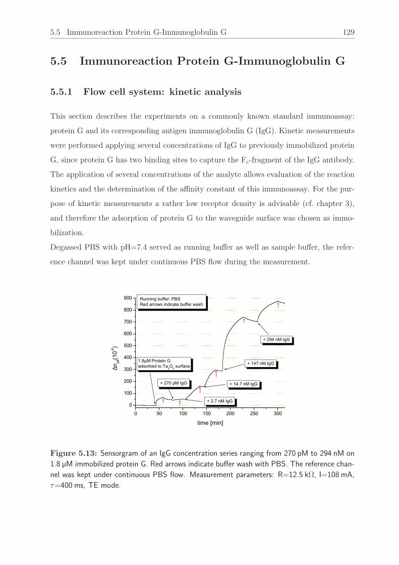
5.5 Immunoreaction Protein G-Immunoglobulin G 129
5.5 Immunoreaction Protein G-Immunoglobulin G
5.5.1 Flow cell system: kinetic analysis
This section describes the experiments on a commonly known standard immunoassay:
protein G and its corresponding antigen immunoglobulin G (IgG). Kinetic measurements
were performed applying several concentrations of IgG to previously immobilized protein
G, since protein G has two binding sites to capture the Fc-fragment of the IgG antibody.
The application of several concentrations of the analyte allows evaluation of the reaction
kinetics and the determination of the affinity constant of this immunoassay. For the pur-
pose of kinetic measurements a rather low receptor density is advisable (cf. chapter 3),
and therefore the adsorption of protein G to the waveguide surface was chosen as immo-
bilization.
Degassed PBS with pH=7.4 served as running buffer as well as sample buffer, the refer-
ence channel was kept under continuous PBS flow during the measurement.
0 50 100 150 200 250 300
0
100
200
300
400
500
600
700
800
900
+ 294 nM IgG
+ 147 nM IgG
+ 14.7 nM IgG
Running buffer: PBSRed arrows indicate buffer wash
+ 2.7 nM IgG
+ 270 pM IgG
1.8µM Protein Gadsorbed to Ta2O5 surface∆n
eff(1
0-6)
time [min]
Figure 5.13: Sensorgram of an IgG concentration series ranging from 270 pM to 294 nM on
1.8 µM immobilized protein G. Red arrows indicate buffer wash with PBS. The reference chan-
nel was kept under continuous PBS flow. Measurement parameters: R=12.5 kΩ, I=108 mA,
τ=400 ms, TE mode.

130 CHAPTER 5 Application measurements
The complete measurement was run in the two-channel flow cell at a flow rate of ≈40 µl/min.
Fig. 5.13 shows the sensorgram of the IgG concentration series on protein G. After mon-
itoring of the PBS baseline for ≈45 min, 1.8 µM protein G in PBS has been applied on
the measurement channel for 15 min until equilibrium, followed by PBS to remove un-
bound protein. Subsequently IgG concentrations of 270 pM, 2.7 nM, 14.7 nM, 147 nM
and 294 nM were injected, each followed by PBS buffer. It can be seen from the sen-
sorgram that the 294 nM-concentration is close to equilibrium, so that the injection of
higher concentrations was not expected to cause further IgG binding. Fig. 5.14a shows
the PBS baseline previous to protein G immobilization, where the inset shows a linear fit
to the baseline to determine signal noise and drift. The signal noise at a sampling rate of
τ=400 ms was determined to 3.1 · 10−8 with a drift of < 1 · 10−6/h. Fig. 5.14b illustrates
a single concentration of 313 pM IgG binding to immobilized protein G, indicating that
the experimental limit of detection lies in the low pM range.
b)a)
0 10 20 30 40 5025
30
35
40
45
PBS
+ 313pM IgG
∆nef
f(10-6
)
time [min]0 10 20 30 40 50
-2
0
2
4
6
8
10
σ=3.1*10-8
drift: 0.5*10-6/h
42,0 42,5 43,0 43,5 44,0 44,5 45,0-0,96
-0,94
-0,92
-0,90
-0,88
-0,86
-0,84
-0,82
-0,80
-0,78
∆nef
f (10-6
)
time [min]
Figure 5.14: a) 45 min-baseline of the protein G - IgG immunoassay. The inset shows a linear
fit to the baseline to determine signal noise and drift. The signal noise at a sampling rate of
τ=400 ms was determined to 3.1 · 10−8 with a drift of < 1 · 10−6/h. b) Single concentration
of 313 pM IgG on immobilized protein G.
From the sensorgram the binding rate constants ka, kd and the affinity constant K have
been obtained as described in chapter 3.4.1. A plot of the end signal values versus the
respective concentration (dose-response-curve), fitted to the Langmuir isotherm, yields
the affinity constant K and the signal change equivalent to the maximum analyte con-
centration. The end signal values are obtained from Fig. 5.13 for each concentration
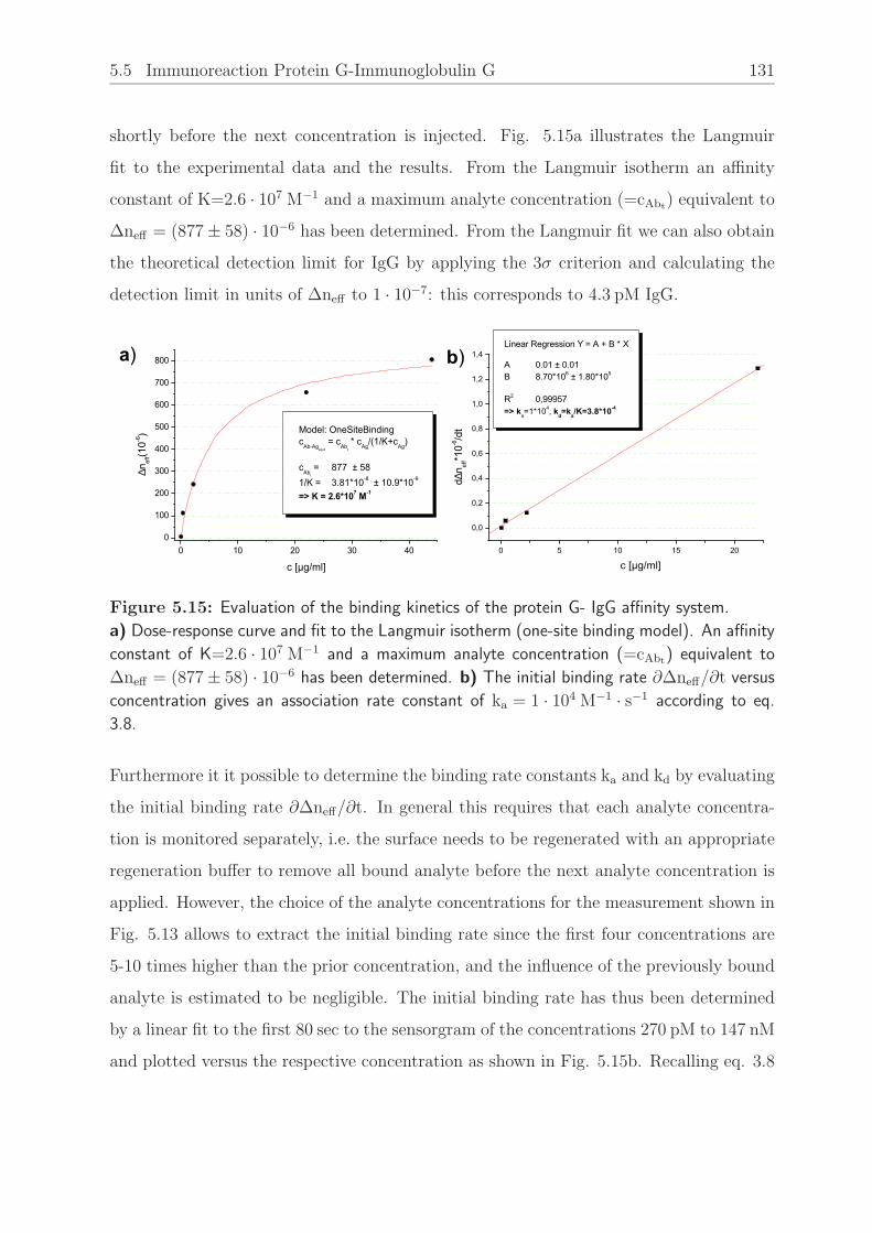
5.5 Immunoreaction Protein G-Immunoglobulin G 131
shortly before the next concentration is injected. Fig. 5.15a illustrates the Langmuir
fit to the experimental data and the results. From the Langmuir isotherm an affinity
constant of K=2.6 · 107 M−1 and a maximum analyte concentration (=cAbt) equivalent to
∆neff = (877 ± 58) · 10−6 has been determined. From the Langmuir fit we can also obtain
the theoretical detection limit for IgG by applying the 3σ criterion and calculating the
detection limit in units of ∆neff to 1 · 10−7: this corresponds to 4.3 pM IgG.
0 5 10 15 20
0,0
0,2
0,4
0,6
0,8
1,0
1,2
1,4Linear Regression Y = A + B * X
A 0.01 ± 0.01B 8.70*106 ± 1.80*105
R2 0,99957=> k
a=1*104, k
d=k
a/K=3.8*10-4
d∆n ef
f*10-6
/dt
c [µg/ml]
b)a)
0 10 20 30 400
100
200
300
400
500
600
700
800
Model: OneSiteBindingc
Ab-Agequil
= cAb
t
* cAg/(1/K+c
Ag)
c
Abt
= 877 ± 581/K = 3.81*10-8 ± 10.9*10-9
=> K = 2.6*107 M-1
∆nef
f(10-6
)
c [µg/ml]
Figure 5.15: Evaluation of the binding kinetics of the protein G- IgG affinity system.
a) Dose-response curve and fit to the Langmuir isotherm (one-site binding model). An affinity
constant of K=2.6 · 107 M−1 and a maximum analyte concentration (=cAbt) equivalent to
∆neff = (877 ± 58) · 10−6 has been determined. b) The initial binding rate ∂∆neff/∂t versus
concentration gives an association rate constant of ka = 1 · 104 M−1 · s−1 according to eq.
3.8.
Furthermore it it possible to determine the binding rate constants ka and kd by evaluating
the initial binding rate ∂∆neff/∂t. In general this requires that each analyte concentra-
tion is monitored separately, i.e. the surface needs to be regenerated with an appropriate
regeneration buffer to remove all bound analyte before the next analyte concentration is
applied. However, the choice of the analyte concentrations for the measurement shown in
Fig. 5.13 allows to extract the initial binding rate since the first four concentrations are
5-10 times higher than the prior concentration, and the influence of the previously bound
analyte is estimated to be negligible. The initial binding rate has thus been determined
by a linear fit to the first 80 sec to the sensorgram of the concentrations 270 pM to 147 nM
and plotted versus the respective concentration as shown in Fig. 5.15b. Recalling eq. 3.8

132 CHAPTER 5 Application measurements
the linear fit yields an association rate constant of ka = 1 · 104 M−1s−1 and with kd = ka
K
a dissociation rate constant of kd = 3.8 · 10−4 s−1. These values for the binding rate con-
stants slightly deviate from experimental values found in literature for this affinity system
(Saha et al., 2003). Calculating the surface coverages for protein G and IgG from the
∆neff-values in Fig. 5.13 and the corresponding molecular weights (cf. chapter 3), we
find 4.1 · 10−15 mol/mm2 protein G and 1.5 · 10−14 mol/mm2 IgG, resulting in a ratio of
1:3.8. Yet the protein G provides only two binding sites for the IgG antibody, so that the
deviation might be explained by a certain amount of unspecifically bound IgG. Therefore
it can be concluded that the binding rate constants slightly differ from literature values
due to this unspecific binding.
The maximum antigen concentration corresponding to an antigen monolayer determined
by the Langmuir fit in Fig. 5.15 has been further experimentally verified as illustrated in
Fig. 5.16, where a high concentration of 250 µg/ml IgG has been injected over immobi-
lized protein G according to the same procedure as described above for the concentration
series. It can be seen that the binding comes close to equilibrium after ≈20 min and a
signal increase of ∆neff = 835 · 10−6 can be attributed to IgG binding.
0 10 20 30 40 50 60 70 80
0
200
400
600
800
PBS on reference channelRed arrow indicates buffer wash
neff,tot. =835*10-6
+ 250µg/ml IgG
Protein G immobilization
∆nef
f(10-6
)
time [min]
Figure 5.16: Binding of 250 µg/ml IgG to immobilized protein G. Red arrow indicates
buffer wash with PBS. The reference channel was kept under continuous PBS flow. Mea-
surement parameters: R=12.5 kΩ, I=107 mA, τ=800 ms, TE mode. A signal increase of
∆neff = 835 · 10−6 indicates the formation of an IgG monolayer.

5.5 Immunoreaction Protein G-Immunoglobulin G 133
5.5.2 Microplate system: parallel detection
The same immunoassay has further been probed on the microplate system in 8-well con-
figuration, which allowed the parallel detection of three different analyte concentrations.
By repeated scans the time-resolved measurement showed all binding events. One well
pair has been kept under buffer as negative control and for drift correction. Fig. 5.17
illustrates the layout of the microplate for this experiment, where wells in row A serves
as reference for the measurement wells in row B.
sample 1: 1.8 nM IgGsample 2: 4.5 nM IgGsample 3: 9.0 nM IgG
Figure 5.17: Microplate layout for protein G-IgG measurement and sample allocation.
A1/B1 serve as negative control and for drift correction.
Before the measurement, the microplate has been cleaned in isopropanol in an ultrasonic
bath for 5 min, rinsed with DI − H2O, dried and inserted in the interferometer system.
Wells A1-A4 and B1 were filled with 100 µl PBS. Wells B2-B4 were filled with 100 µl pro-
tein G in PBS with a concentration of 100 µg/ml and incubated for 30 min, followed by 5x
rinsing with 100 µl PBS. Subsequently wells B2-B4 were filled with 100 µl pure PBS and
100 µl of 4.5 nM IgG in PBS added to B2, 9.0 nM IgG in PBS added to B3 and 18.0 nM
IgG in PBS added to B4 and mixed, so that each well contained half of the concentration
added (cf. Fig. 5.17). Now the scanning and readout of the microplate was started and
each well pair monitored for 5 sec before moving to the next well pair, followed by an idle
period of 40 sec, so that data values for each well pair were obtained in 60 sec-intervals.
Fig. 5.18 shows the measurement results. In wells A1/B1 a baseline with a signal drift
of ∆neff = 2.1 · 10−4/h can be observed, whereas in wells A2-A4/B2-B4 IgG binds to the
immobilized protein G (association phase). The measurement data for these wells were
corrected for drift, i.e. the A1/B1-baseline subtracted from the original data. The cor-
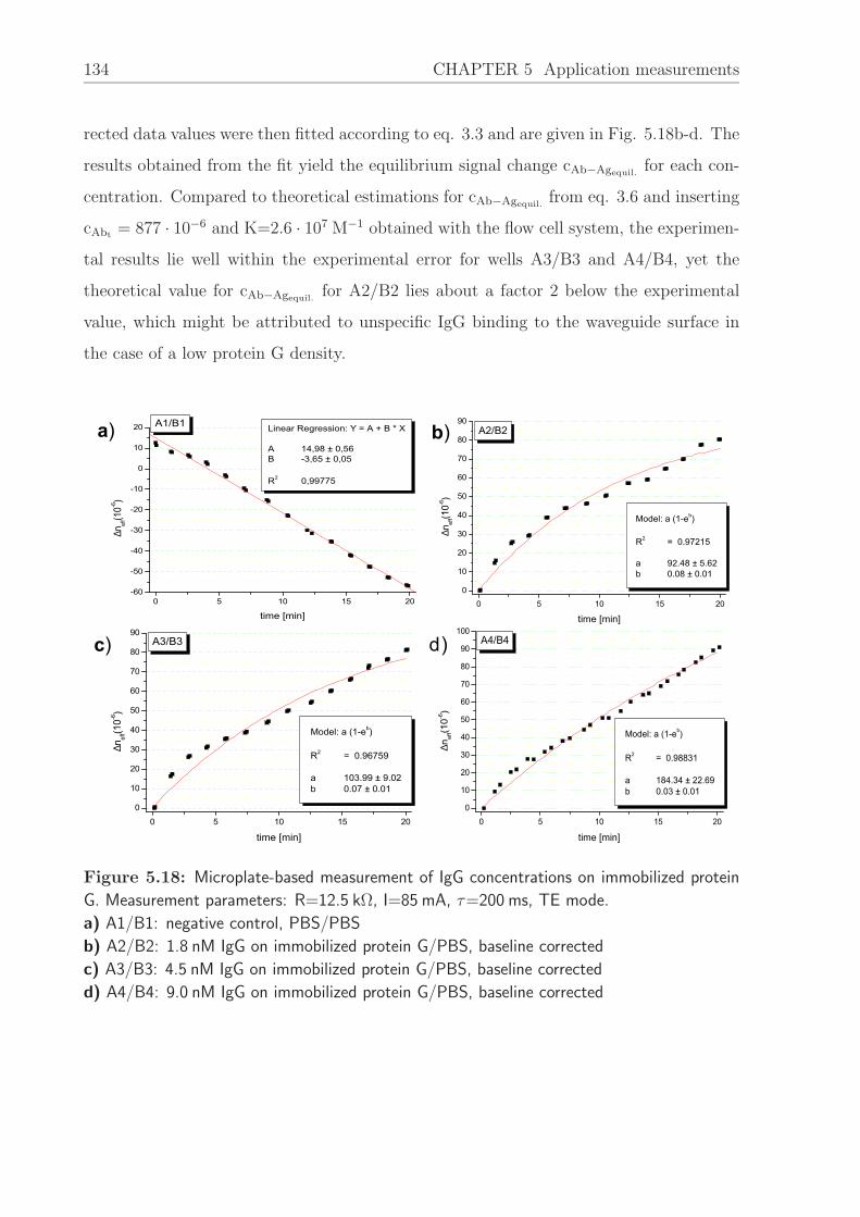
134 CHAPTER 5 Application measurements
rected data values were then fitted according to eq. 3.3 and are given in Fig. 5.18b-d. The
results obtained from the fit yield the equilibrium signal change cAb−Agequil.for each con-
centration. Compared to theoretical estimations for cAb−Agequil.from eq. 3.6 and inserting
cAbt= 877 · 10−6 and K=2.6 · 107 M−1 obtained with the flow cell system, the experimen-
tal results lie well within the experimental error for wells A3/B3 and A4/B4, yet the
theoretical value for cAb−Agequil.for A2/B2 lies about a factor 2 below the experimental
value, which might be attributed to unspecific IgG binding to the waveguide surface in
the case of a low protein G density.
0 5 10 15 20-60
-50
-40
-30
-20
-10
0
10
20 Linear Regression: Y = A + B * X
A 14,98 ± 0,56B -3,65 ± 0,05
R2 0,99775
A1/B1
∆nef
f(10-6
)
time [min]
0 5 10 15 200
10
20
30
40
50
60
70
80
90
100
Model: a (1-eb)
R2 = 0.98831 a 184.34 ± 22.69b 0.03 ± 0.01
A4/B4
∆nef
f(10-6
)
time [min]0 5 10 15 20
0
10
20
30
40
50
60
70
80
90
Model: a (1-eb)
R2 = 0.96759 a 103.99 ± 9.02b 0.07 ± 0.01
A3/B3
∆nef
f(10-6
)
time [min]
0 5 10 15 20
0
10
20
30
40
50
60
70
80
90
Model: a (1-eb)
R2 = 0.97215 a 92.48 ± 5.62b 0.08 ± 0.01
A2/B2∆n
eff(1
0-6)
time [min]
d)c)
b)a)
Figure 5.18: Microplate-based measurement of IgG concentrations on immobilized protein
G. Measurement parameters: R=12.5 kΩ, I=85 mA, τ=200 ms, TE mode.
a) A1/B1: negative control, PBS/PBS
b) A2/B2: 1.8 nM IgG on immobilized protein G/PBS, baseline corrected
c) A3/B3: 4.5 nM IgG on immobilized protein G/PBS, baseline corrected
d) A4/B4: 9.0 nM IgG on immobilized protein G/PBS, baseline corrected

5.6 Immunoreaction Protein A-Immunoglobulin G 135
5.6 Immunoreaction Protein A-Immunoglobulin G
In addition to the immunoassay protein G-IgG, the immunoassay protein A-IgG has been
studied in order to obtain information about the binding kinetics and the binding rate
constants. The experimental procedure is identical to the protein G measurement on the
flow cell system described above. First, protein A is adsorbed to the waveguide surface,
and subsequently a concentration series ranging from 2.9 nM to 576 nM was applied to the
immobilized protein A, each concentration followed by PBS to remove unbound analyte.
Degassed PBS with pH=7.4 served as running buffer as well as sample buffer, the refer-
ence channel was kept under continuous PBS flow during the measurement. The complete
measurement was run in the two-channel flow cell at a flow rate of ≈83 µl/min. Fig. 5.19
shows the sensorgram of the IgG concentration series on protein A. After monitoring of
0 20 40 60 80 100 1200
200
400
600
800
1000 Running buffer: PBSRed arrows indicate buffer wash
+576nM IgG
+288nM IgG
+144nM IgG
+58nM IgG+29nM IgG
+5.8nM IgG
+2.9nM IgG
2.38µM Protein A adsorbed on Ta2O5 surface
∆nef
f(10-6
)
time [min]
Figure 5.19: Sensorgram of an IgG concentration series ranging from 2.9 nM to 576 nM
on 2.38 µM immobilized protein A. Red arrows indicate buffer wash with PBS. The refer-
ence channel was kept under continuous PBS flow. Measurement parameters: R=12.5 kΩ,
I=108 mA, τ=200 ms, TE mode.
the PBS baseline for ≈15 min, 2.38 µM protein A in PBS has been applied on the mea-
surement channel for 7 min, followed by PBS to remove unbound protein. Subsequently
IgG concentrations of 2.9 nM, 5.8 nM, 29 nM, 58 nM, 144 nM, 288 nM and 576 nM were
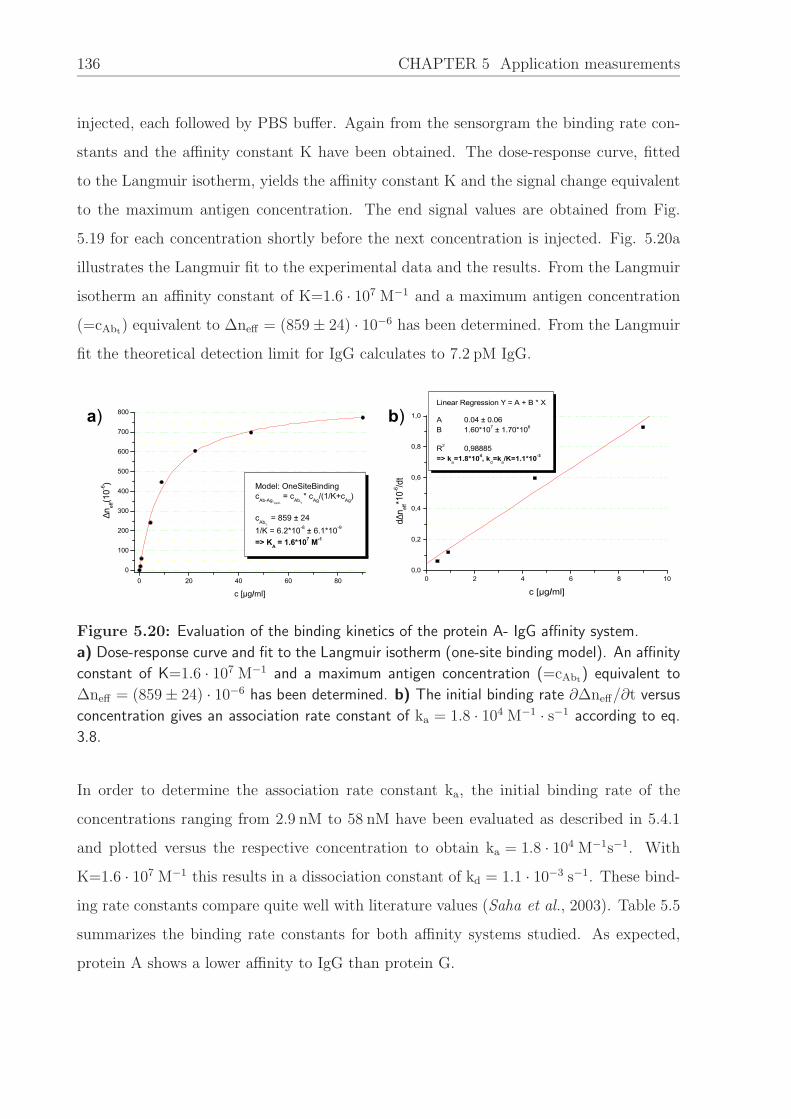
136 CHAPTER 5 Application measurements
injected, each followed by PBS buffer. Again from the sensorgram the binding rate con-
stants and the affinity constant K have been obtained. The dose-response curve, fitted
to the Langmuir isotherm, yields the affinity constant K and the signal change equivalent
to the maximum antigen concentration. The end signal values are obtained from Fig.
5.19 for each concentration shortly before the next concentration is injected. Fig. 5.20a
illustrates the Langmuir fit to the experimental data and the results. From the Langmuir
isotherm an affinity constant of K=1.6 · 107 M−1 and a maximum antigen concentration
(=cAbt) equivalent to ∆neff = (859 ± 24) · 10−6 has been determined. From the Langmuir
fit the theoretical detection limit for IgG calculates to 7.2 pM IgG.
0 2 4 6 8 100,0
0,2
0,4
0,6
0,8
1,0
Linear Regression Y = A + B * X
A 0.04 ± 0.06B 1.60*107 ± 1.70*106
R2 0,98885=> k
a=1.8*104, k
d=k
a/K=1.1*10-3
d∆n ef
f*10-6
/dt
c [µg/ml]
b)a)
0 20 40 60 800
100
200
300
400
500
600
700
800
Model: OneSiteBinding c
Ab-Ag,equil.
= cAb,
t * c
Ag/(1/K+c
Ag)
c
Ab,t = 859 ± 24
1/K = 6.2*10-8 ± 6.1*10-9
=> KA = 1.6*107 M-1
∆nef
f(10-6
)
c [µg/ml]
Figure 5.20: Evaluation of the binding kinetics of the protein A- IgG affinity system.
a) Dose-response curve and fit to the Langmuir isotherm (one-site binding model). An affinity
constant of K=1.6 · 107 M−1 and a maximum antigen concentration (=cAbt) equivalent to
∆neff = (859 ± 24) · 10−6 has been determined. b) The initial binding rate ∂∆neff/∂t versus
concentration gives an association rate constant of ka = 1.8 · 104 M−1 · s−1 according to eq.
3.8.
In order to determine the association rate constant ka, the initial binding rate of the
concentrations ranging from 2.9 nM to 58 nM have been evaluated as described in 5.4.1
and plotted versus the respective concentration to obtain ka = 1.8 · 104 M−1s−1. With
K=1.6 · 107 M−1 this results in a dissociation constant of kd = 1.1 · 10−3 s−1. These bind-
ing rate constants compare quite well with literature values (Saha et al., 2003). Table 5.5
summarizes the binding rate constants for both affinity systems studied. As expected,
protein A shows a lower affinity to IgG than protein G.

5.7 Biotinylated Cytochrome c: Comparison with BIACORE 1000 technology 137
A calculation of the surface coverages for this affinity system yields 9.0 · 10−15 mol/mm2
protein A binding 1.4 · 10−14 mol/mm2 IgG, equivalent to a reaction stoichiometry of
≈1.5:1 IgG to protein A. Protein A has a binding capacity of four Fc-fragments of the
IgG antibody, i.e. higher than the experimentally determined stoichiometry. This can be
explained by the fact that not all four binding sites can be available for IgG binding when
the protein A is immobilized to the surface.
Affinity system ka [M−1 · s−1] kd [s−1] K [M−1]
protein G-IgG 1.0 · 104 3.8 · 10−4 2.6 · 107
protein A-IgG 1.8 · 104 1.1 · 10−3 1.6 · 107
Table 5.5: Experimentally determined binding constants for the affinity systems protein
G-IgG and protein A-IgG.
5.7 Biotinylated Cytochrome c:
Comparison with BIACORE 1000 technology
In section 5.2 and 5.3 the surface chemistry using the affinity system biotin-streptavidin
and test measurements with the interferometric biosensor have been described. This
section provides measurements with biotinylated cytochrome c, a small mitochondrial
protein, on the streptavidin-funtionalized surface. The same experiment has been per-
formed on the BIACORE 1000 Upgrade in order to compare the interferometric biosensor
to a commercially available system. The measurement on the BIACORE was conducted
in cooperation with the Institute for Biology III of the University of Freiburg. The bi-
otinylated cytochrome c was kindly provided by the Fraunhofer IGB in Stuttgart.
The interferometer measurement has been performed on the flow cell system at a flow
rate of ≈83 µl/min using degassed PBS as running buffer and as reference. A biotinylated
sensor chip was inserted into the interferometric biosensor and a PBS baseline monitored
previous to the injection of 50 µg/ml SAv on the measurement channel. After buffer
wash with PBS the binding of 17.5 µg/ml biotinylated cytochrome c to SAv was mon-
itored. Fig. 5.21 shows the sensorgram of the binding reaction. A signal increase of

138 CHAPTER 5 Application measurements
∆neff = 797 · 10−6 indicates SAv binding, a signal increase of ∆neff = 219 · 10−6 can be
attributed to cytochrome c binding.
0 10 20 30 40 50 60 70 80
0
200
400
600
800
1000
n eff(1
0-6)
time [min]
PBS baseline
+ 50µg/ml SAv
PBS
+ 17.5µg/ml cytochrome C
Figure 5.21: Sensorgram of biotinylated cytochrome c binding to immobilized SAv. Mea-
surement performed with the interferometric biosensor IBS 201 at following parameters:
R=12.5 kΩ, I=120 mA, τ=400 ms, TE mode.
For comparison, the binding of the same concentration of biotinylated cytochrome c has
been studied on the BIACORE 1000 Upgrade using an SA sensor chip supplied by BIA-
CORE. The gold surface of this sensor chip is coated with a carboxymethylated dextran
matrix pre-immobilized with streptavidin. The measurement was performed with de-
gassed PBS as running buffer and reference at a flow rate of ≈10 µl/min and a sampling
rate of 1 Hz, using a new sensor chip. After monitoring of a PBS baseline, as shown in
Fig. 5.22, the binding of cytochrome c was detected and a signal increase of 2821 R.U.
determined.
Both sensorgrams have been evaluated with respect to signal noise, baseline drift and the
signal increase due to cytochrome c binding. Table 5.6 illustrates the comparison of the
measurement data from both systems. The baseline drift as well as the signal noise is
higher in the BIACORE compared to the interferometer system, and a deviation of the
experimental values from the specifications for the BIACORE could be observed. The
signal-to-noise ratio of cytochrome c binding was calculated to 1.56 · 104 for the IBS 201
and 3.1 · 103 for the BIACORE by dividing the signal increase by the baseline noise.

5.7 Biotinylated Cytochrome c: Comparison with BIACORE 1000 technology 139
0 2 4 6 8 10 12 14 16 18
15500
16000
16500
17000
17500
18000
18500
R.U.,tot = 2821
PBS
+ 17.5µg/ml cytochrome C
PBS baseline
R.U
.
time [min]
Figure 5.22: Sensorgram of biotinylated cytochrome c binding to immobilized SAv. Mea-
surement performed with the BIACORE 1000 Upgrade at a sampling rate of 1 Hz.
The effective signal changes obtained from the interferometer sensorgram again provide
information about the stoichiometry of the binding reaction. Ideally the immobilized
streptavidin captures two biotinylated cytochrome c molecules. Assuming M=66 kDa
for SAv calculates with ∆neff = 797 · 10−6 to 3.36 · 10−14 mol/mm2, a signal change of
∆neff = 219 · 10−6 for a 12.5 kDa cytochrome c yields 4.90 · 10−14 mol/mm2, resulting in
an experimentally determined stoichiometry of 1:1.45.
IBS 201 BIACORE 1000U
Refractive index range 1.33 − 1.42 1.33 − 1.36
Baseline drift < ±1.0 · 10−6/h < ± 18 R.U./h spec.
(=17.6 R.U.) (=1.02 · 10−6/h)
Exp.: 109 R.U./h
Noise < 1.0 · 10−8 sd at 2.5 Hz < 0.6 R.U. sd at 1 Hz spec.
(=0.176 R.U. sd) (=3.41 · 10−8)
Exp.: 0.91 R.U. sd at 0.1 Hz
SNR from meas. data 1.56 · 104 3.1 · 103
Table 5.6: Comparison of measurement data for cytochrome c binding: IBS 201 and BIA-
CORE 1000U

140 CHAPTER 5 Application measurements
5.8 Biotinylated α-NPT IgG antigen:
Comparison with BIACORE 2000 technology
This section describes the investigation of an antibody-antigen system commonly used for
a protein production process at the Novartis Institute for Biomedical Research in Basel,
Switzerland (NIBR). All measurements were performed on a BIACORE 2000 sensor sys-
tem and the IBS 201 and conducted in cooperation with the NIBR, where the monitoring
of recombinant proteins is an essential tool in the development of novel proteins for ther-
apeutics. Common techniques for protein expression analysis and protein purification are
SDS-PAGE or Western blot analysis. Yet these methods are time consuming and labor
intensive and therefore not suited for a high throughput. One alternative allowing higher
throughput are automated ELISAs. A list of these current technologies used for protein
expression analysis can be found in (Baker et al., 2002). A more detailed description of
the methods is e.g. provided in (Davies , 2001).
A large variety of tags is to date available for labeling recombinant proteins (Stevens ,
2000). In general, proteins carrying a large tag can be easily detected by ELISA, yet
large tags can also interfere with the functionality of the protein. Therefore the focus at
NIBR is the development of small tags and the detection of recombinant proteins express-
ing these tags. A fully automated competitive ELISA as general detection method for the
quatitation of recombinant proteins has also been developed at NIBR. Yet a competitive
ELISA has the intrinsic problem that any interference from the matrix can lead to a false
positive signal, i.e. is misinterpreted as high protein concentration.
As an alternative to the competitive ELISA, optical biosensors allow the direct detec-
tion of the protein by its corresponding immobilized antibody. In the experiments de-
scribed in this section, a recombinant standard protein of 21 kDa (E2-NPT expressed by
E. coli), carrying a small tag developed at NIBR consisting of four amino acids, NPT
(N ovartis Proprietary Tag), is detected by a biotinylated monoclonal mouse IgG directed
against this tag (α-NPT IgG). The α-NPT IgG binds the antigen with the Fab-fragments,
i.e. two binding sites per antibody are available for antigen binding. In a first experiment,
a concentration series of the protein in PBS/BSA as sample buffer is detected by the im-

5.8 Biotinylated α-NPT IgG antigen: Comparison with BIACORE 2000 technology 141
mobilized antibody to determine the affinity constant of the system. Further experiments
using cell lysate from E. coli show the suitability of both biosensor systems to detect the
same protein in a more complex matrix. The detection of a ligand, e.g. a protein, directly
from a cell lysate is of great importance in pharmaceutical screening studies, where the
binding of new targets is investigated. Label-free detection methods are especially suited
when screening for new targets due to possible side effects of labeling. Yet the assay has
to be deliberately chosen to minimize unspecific binding effects from cell lysate compo-
nents which might lead to a misinterpretation of the biosensor data. In the following the
measurement data of the biosensor systems are compared and discussed.
All waveguide chips used for the IBS 201 were silanized according to the protocol in section
5.1.2 and functionalized via biotin linking to provide a streptavidin surface. For the BIA-
CORE system, a sensor chip SA was obtained from BIACORE. This sensor chip is coated
with a carboxymethylated dextran matrix pre-immobilized with streptavidin. Fig. 5.23 il-
lustrates the surface chemistries of both sensor chips, which differ in one important aspect:
while the silane chemistry on the IBS waveguide surface provides a two-dimensional strep-
tavidin surface, the dextran matrix of the BIACORE sensor provides a three-dimensional
structure where the streptavidin molecules are exposed in arbitrary orientation, resulting
in a higher binding capacity for the biotinylated reagents.
Figure 5.23: Comparison of the sensor chip surfaces. a) The dextran matrix on the BIA-
CORE sensor chip SA provides a three-dimensional structure pre-immobilized with SAv. b)
Silane chemistry on the IBS waveguide chip providing a two-dimensional SAv surface.
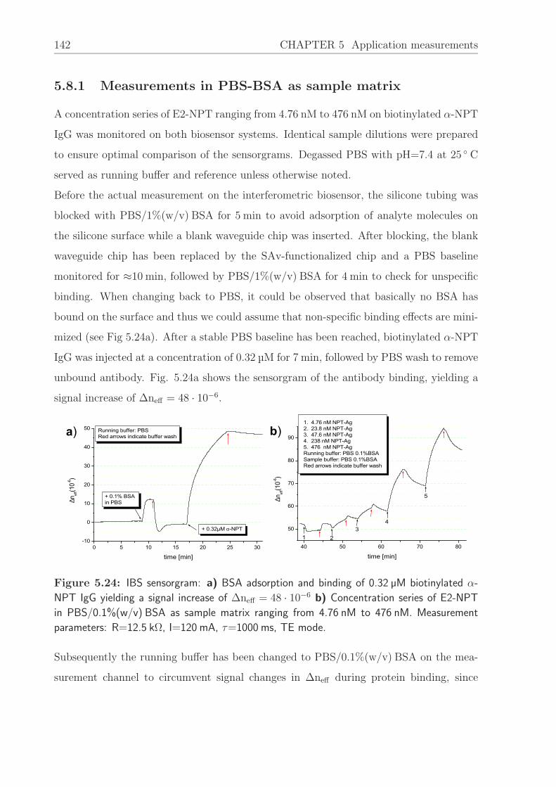
142 CHAPTER 5 Application measurements
5.8.1 Measurements in PBS-BSA as sample matrix
A concentration series of E2-NPT ranging from 4.76 nM to 476 nM on biotinylated α-NPT
IgG was monitored on both biosensor systems. Identical sample dilutions were prepared
to ensure optimal comparison of the sensorgrams. Degassed PBS with pH=7.4 at 25 C
served as running buffer and reference unless otherwise noted.
Before the actual measurement on the interferometric biosensor, the silicone tubing was
blocked with PBS/1%(w/v) BSA for 5 min to avoid adsorption of analyte molecules on
the silicone surface while a blank waveguide chip was inserted. After blocking, the blank
waveguide chip has been replaced by the SAv-functionalized chip and a PBS baseline
monitored for ≈10 min, followed by PBS/1%(w/v) BSA for 4 min to check for unspecific
binding. When changing back to PBS, it could be observed that basically no BSA has
bound on the surface and thus we could assume that non-specific binding effects are mini-
mized (see Fig 5.24a). After a stable PBS baseline has been reached, biotinylated α-NPT
IgG was injected at a concentration of 0.32 µM for 7 min, followed by PBS wash to remove
unbound antibody. Fig. 5.24a shows the sensorgram of the antibody binding, yielding a
signal increase of ∆neff = 48 · 10−6.
40 50 60 70 80
50
60
70
80
90
1. 4.76 nM NPT-Ag2. 23.8 nM NPT-Ag3. 47.6 nM NPT-Ag4. 238 nM NPT-Ag5. 476 nM NPT-AgRunning buffer: PBS 0.1%BSASample buffer: PBS 0.1%BSARed arrows indicate buffer wash
5
43
21
∆nef
f(10-6
)
time [min]
b)a)
0 5 10 15 20 25 30-10
0
10
20
30
40
50 Running buffer: PBSRed arrows indicate buffer wash
+ 0.32µM α-NPT
+ 0.1% BSA in PBS∆n
eff(1
0-6)
time [min]
Figure 5.24: IBS sensorgram: a) BSA adsorption and binding of 0.32 µM biotinylated α-
NPT IgG yielding a signal increase of ∆neff = 48 · 10−6 b) Concentration series of E2-NPT
in PBS/0.1%(w/v) BSA as sample matrix ranging from 4.76 nM to 476 nM. Measurement
parameters: R=12.5 kΩ, I=120 mA, τ=1000 ms, TE mode.
Subsequently the running buffer has been changed to PBS/0.1%(w/v) BSA on the mea-
surement channel to circumvent signal changes in ∆neff during protein binding, since

5.8 Biotinylated α-NPT IgG antigen: Comparison with BIACORE 2000 technology 143
the sample buffer for the protein dilutions consists of PBS/0.1%(w/v) BSA. It should
be noted here that only 0.1%(w/v) BSA was added to the PBS, since from experience
higher BSA concentrations are likely to cause air bubbles during the measurement that
might distort the signal, and 0.1%(w/v) BSA seemed sufficient to minimize unspecific
binding effects. Fig. 5.24b illustrates the binding of E2-NPT to biotinylated α-NPT IgG
in concentrations of 4.76 nM, 23.8 nM, 47.6 nM, 238 nM and 476 nM, each followed by
PBS/0.1%(w/v) BSA to remove unbound antigen. Both the injection time and the buffer
wash was set to 240 sec. The concentration series was followed by a regeneration pulse with
a phosphate buffer (10 mM H3PO4 adjusted to pH=2 with NaOH) for 30 sec to elute the
bound antigen. To investigate the reproducibility of antigen binding, 238 nM E2-NPT in
PBS/0.1%(w/v) BSA has been injected three times with subsequent PBS/0.1%(w/v) BSA
wash and 30 sec regeneration as illustrated in Fig. 5.25a. Fig. 5.25b shows the evaluated
binding and regeneration levels, indicating that after four regeneration steps the binding
level approximates the regeneration level, i.e. it can be assumed that the surface is stable.
120 130 140 150 160 170 180 190
-80
-60
-40
-20
0
20
40
60
Red arrows indicate buffer washGreen arrows indicate regeneration
+ 238 nM NPT-Ag
+ 238 nM NPT-Ag
+ 238 nM NPT-Ag
∆nef
f(10-6
)
time [min]1 2 3 4 5
0
2
4
6
8
10
12
14
16 Binding level Regeneration level
Repeated binding of 238 nM NPT-Ag
∆nef
f(10-6
)
# of regenerations
b)a)
Figure 5.25: a) IBS sensorgram of a regeneration cycle: repeated binding of 238 nM E2-
NPT and subsequent regeneration with phophate buffer (see text) b) Binding and regeneration
levels. After four regenerations the binding level approximates the regeneration level and a
stable surface is reached.
Fig. 5.26 shows the corresponding measurement on the BIACORE system, using antigen
concentrations ranging from 4.76 nM to 238 nM. In this experiment, PBS served as run-
ning buffer and PBS/0.1%(w/v) BSA as sample buffer, thus an additional signal increase

144 CHAPTER 5 Application measurements
during antigen injection can be observed due to a difference in the refractive index of
the buffer solutions. The immobilization of 0.32 µM α-NPT IgG was performed accord-
ing to the aforementioned procedure on the IBS system, resulting in a signal increase of
1818 R.U. Each antigen concentration was again injected for 240 sec, followed by PBS for
240 sec. A regeneration with phosphate buffer eluted the bound antigen. For the evalua-
tion of the effective signal increase the signal values obtained 15 sec after PBS injection
were taken and plotted versus the respective concentration as depicted in Fig. 5.27a, com-
pared with the end signal values obtained with the interferometric biosensor (Fig. 5.27b).
Both data sets were fitted to a one-site binding model (Langmuir isotherm) to obtain
the affinity constant of the α-NPT IgG - E2-NPT affinity system. With the BIACORE
sensor, an affinity constant of K=1.35 · 107 M−1 and a maximum antigen
0 500 1000 1500 2000 2500 300017800
18000
18200
18400
18600
18800
19000
19200
19400
19600
19800
20000
1. 0.32 µM α-NPT2. PBS 0.1%BSA3. 4.76 nM NPT-Ag4. 23.8 nM NPT-Ag5. 47.6 nM NPT-Ag6. 238 nM NPT-Ag7. 30 sec Reg. 10mM pH2-bufferRed arrows indicate buffer wash
7
65432
1
R.U
.
time (sec)
Figure 5.26: BIACORE sensorgram of α-NPT IgG immobilization and the E2-NPT concen-
tration series ranging from 4.76 nM to 238 nM. Measurement performed at a sampling rate of
1 Hz and a flow rate of ≈80 µl/min.
concentration equivalent to 149.77 ± 9.66 has been determined. The IBS data yield an
affinity constant of K=3.83 · 106 M−1 and a maximum antigen concentration equating
∆neff = (22.81 ± 1.52) · 10−6. The values for the affinity constant thus differ by a factor
≈3.5 from another, which lies well within the experimental error. Applying the 3σ-

5.8 Biotinylated α-NPT IgG antigen: Comparison with BIACORE 2000 technology 145
criterion, the detection limit is 12 nM E2-NPT (IBS) or 45 nM E2-NPT (BIACORE).
The flow rate of the measurement has been set to 83 µl/min for both biosensor systems
to obtain a reasonable antibody load and antigen binding within the given time intervals
despite the differently sized flow cells. With a flow cell volume of 3 µl per channel in
the IBS compared to 60 nl per channel in the BIACORE, the flow is considerably faster
in the BIACORE flow cell, which has crucial effects on the total antibody load and the
kinetics of antigen binding. As it can be seen in Fig. 5.24 and Fig. 5.26, an antibody load
of 1818 R.U. being equal to 1.82 ng/mm2 exceeds the antibody load of ∆neff = 48 · 10−6
corresponding to 0.14 ng/mm2 by about a factor 13, using a refractive index of 1.38. 1
b)a)
0 50 100 150 200 2500
20
40
60
80
100
120
Model: OneSiteBinding
cAb-Agequil.
=cAbt
* cAg/(1/K+cAg) cAb
t
149.77 ± 9.661/K 7.42*10-8 ± 1.22*10-8
=> K=1.35*107 M-1
R.U
.
c [nM]0 100 200 300 400 500
0
2
4
6
8
10
12
14
16
Model: OneSiteBinding cAb-Ag
equil.
=cAbt
* cAg/(1/K+cAg) cAb
t
22.81 ± 1.521/K 2.61*10-7 ± 3.91*10-8
=> K=3.83*106 M-1
∆nef
f(10-6
)
c[nM]
Figure 5.27: Langmuir fit of the α-NPT IgG - E2-NPT binding data. Sample ma-
trix: PBS-0.1%BSA. a) BIACORE data yield an affinity constant of K=1.35 · 107 M−1
and a maximum antigen concentration equivalent to 149.77 ± 9.66 R.U. b) IBS data yield
an affinity constant of K=3.83 · 106 M−1 and a maximum antigen concentration equating
∆neff = (22.81 ± 1.52) · 10−6.
Furthermore the flow rate combined with the flow cell size of the IBS results in mass-
transport limited conditions, therefore the association rate constant and dissociation rate
constant could not be reliably determined. Nevertheless we considered the flow rate as
reasonable to detect low concentrations of the antigen while keeping the total sample
consumption low.
1In the following a refractive index of 1.38 for antibody layers and 1.45 for antigen layers is used.
Surface coverages are calculated using 1pg/mm2=1 R.U.
Signals given in R.U. are related with measurements on the BIACORE 2000 and signals given in ∆neff
are related to the interferometric biosensor.

146 CHAPTER 5 Application measurements
A calculation of the surface coverages for the α-NPT IgG - E2-NPT affinity system yields
1.17 · 10−14 mol/mm2 α-NPT IgG binding 7.13 · 10−15 mol/mm2 E2-NPT on the BIA-
CORE resulting in a stoichiometry of 1.6:1, i.e. less antigen is bound than antibody bind-
ing sites are available. The IBS data yield surface coverages of 8.54 · 10−16 mol/mm2 α-
NPT IgG binding 3.02 · 10−15 mol/mm2 E2-NPT giving a stoichiometry of 1:3.5, although
only two binding sites are available. This indicates that some antigen is unspecifically
bound.
5.8.2 Measurements in cell lysate as sample matrix
We furthermore studied the α-NPT IgG - E2-NPT affinity system in cleared E. coli cell
lysate as sample matrix. The E. coli lysate was produced at the Biomolecular Production
Unit of NIBR and prepared by incubating E. coli pellets for 30 min in PBS pH 7.4 at
room temperature under addition of lysozyme and benzonase to facilitate cell lysis. The
cell suspension was then frozen at -80 C for 1 h and the lysate cleared after thawing by
centrifugation at 5000 x g to remove cell debris.
According to the measurements in PBS/BSA a concentration series of E2-NPT ranging
from 4.76 nM to 476 nM was detected by 0.32 µM immobilized biotinylated α-NPT IgG
on both biosensor systems, using identical sample dilutions for optimal comparison. De-
gassed PBS with pH=7.4 at 25 C served as running buffer and reference.
Previous to the measurement on the IBS 201 the silicone tubing was blocked with 1.5 ml
PBS/1%(w/v) BSA while a blank chip was inserted. After replacing the blank chip by the
SAv-functionalized chip, a PBS baseline was monitored for ≈15 min. Fig. 5.28 shows the
sensorgram of the measurement. Following the immobilization of 0.32 µM α-NPT IgG,
both the measurement channel (2 x) and the reference channel (1 x) were blocked with
pure cell lysate to avoid unspecific binding of cell lysate components that might distort
the analyte signal. The level of unspecific binding (∆neff = 50 · 10−6) was approximately
equal on both channels, indicating a stable surface. The signal increase of ∆neff = 43 · 10−6
resulting from antibody binding compares well to the previous measurement, indicating
a good reproducibility of the surface chemistry and immobilization technique. The E2-

5.8 Biotinylated α-NPT IgG antigen: Comparison with BIACORE 2000 technology 147
0 20 40 60 80 100 120 140 160-800
-600
-400
-200
0
200
400
600
800
1000
Running buffer: PBSRed arrows indicate lysate injection for 30secGreen arrows indicate regeneration for 30 sec
1. 0.32µM α-NPT2. 4.76 nM NPT-Ag3. 23.8 nM NPT-Ag4. 47.6 nM NPT-Ag5. 238 nM NPT-Ag6. 476 nM NPT-Ag
66654321∆n
eff(1
0-6)
time [min]
Figure 5.28: IBS sensorgram of an E2-NPT concentration series ranging from 4.76 nM
to 476 nM on α-NPT IgG in E. coli lysate as sample matrix. Measurement parameters:
R=12.5 kΩ, I=120 mA, τ=1000 ms, flow rate 83 µl/min, TE mode.
NPT concentrations (4.76 nM, 23.8 nM, 47.6 nM, 238 nM and 476 nM) in cell lysate were
applied according to the above mentioned measurement in 240 sec intervals with PBS as
running buffer to remove unbound analyte. The very high signal changes during sample
injection are due to the difference in refractive index of PBS compared to the cell lysate.
Using cell lysate as running medium to eliminate the signal changes would not be feasible
since in screening applications an unknown target molecule is directly detected from cell
lysate. Therefore the signal reached 15 sec after PBS injection were taken for further
evaluation as illustrated in Fig. 5.29b.
Fig. 5.30 shows the corresponding measurement of the E2-NPT concentration series from
4.76 nM to 476 nM on the BIACORE system and an enlargement of the sensorgram where
the signal values for data evaluation are indicated (15 sec after PBS wash). The effec-
tive signal increases due to antigen binding were obtained from both sensorgrams and
plotted versus their respective concentration in Fig. 5.31. Both data sets were fitted to
the one-site binding model (Langmuir isotherm) to obtain the affinity constant of the
α-NPT IgG - E2-NPT affinity system. With the BIACORE sensor, an affinity constant

148 CHAPTER 5 Application measurements
0 10 20 30 40 50 60670
680
690
700
710
5
54
3
2
1
1. 4.76 nM NPT-Ag2. 23.8 nM NPT-Ag3. 47.6 nM NPT-Ag4. 238 nM NPT-Ag5. 476 nM NPT-Ag
∆nef
f(10-6
)
time [min]0 10 20 30 40 50 60
30
40
50
60
70
80
90
100
5
6
5
43
2
1
1. 4.76 nM NPT-Ag2. 23.8 nM NPT-Ag3. 47.6 nM NPT-Ag4. 238 nM NPT-Ag5. 476 nM NPT-Ag6. Phosphate buffer regenerationGreen arrows indicate pts of evaluation
∆nef
f(10-6
)
time [min]
a) b)
Figure 5.29: IBS sensorgram of the E2-NPT concentration series in E. coli lysate, enlarged
a) Signal responses after sample injection b) End signals reached after PBS injection. Green
arrows indicate points for evaluation.
of K=1.07 · 108 M−1 and a maximum antigen concentration equivalent to 157.87 ± 16.10
has been determined. The IBS data yield an affinity constant of K=1.06 · 108 M−1 and a
maximum antigen concentration equating ∆neff = (41.87 ± 5.12) · 10−6. The affinity con-
stant obtained with the IBS sensor compares very well to the affinity constant obtained
with the BIACORE sensor, but both values differ from the affinity constants measured
in PBS/0.1%(w/v) BSA as sample matrix. This might be explained by the more complex
matrix environment of a cell lysate (Hartmann, 2005). This finding is also supported by
the calculation of the surface coverages for the α-NPT IgG - E2-NPT affinity system: the
BIACORE data yield 1.34 · 10−15 mol/mm2 α-NPT IgG binding 1.19 · 10−15 mol/mm2 E2-
NPT on the BIACORE resulting in a stoichiometry of 1.1:1. The IBS data yield surface
coverages of 9.5 · 10−16mol/mm2 α-NPT IgG binding 5.6 · 10−15 mol/mm2 E2-NPT giving
a stoichiometry of ≈1:6. Recalling that two binding sites on the antibody are available for
antigen binding, the BIACORE data indicate that approximately one antigen molecule
is bound per immobilized antibody, and the IBS data implies six antigen molecules per
antibody, i.e. unspecific binding might have occured.
Apart from the blocking steps with cell lysate previous to antigen detection, a way to
reduce the effects of unspecific binding is a simultaneous antigen injection over both
channels possible with the IBS (one-channel configuration). Fig. 5.32 shows a mea-
surement obtained with the IBS, where 0.32 µM α-NPT IgG has been immobilized as
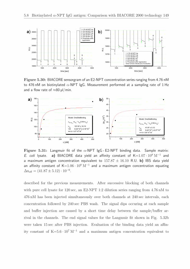
5.8 Biotinylated α-NPT IgG antigen: Comparison with BIACORE 2000 technology 149
1000 2000 3000 4000
19600
19700
19800
19900
20000
6
1. 4.76 nM NPT-Ag2. 23.8 nM NPT-Ag3. 47.6 nM NPT-Ag4. 238 nM NPT-Ag5. 476 nM NPT-Ag6. Phosphate buffer regenerationGreen arrows indicate pts of evaluation
5
6
54
32
1
R.U
.
time [sec]1000 2000 3000 4000 5000
18000
20000
22000
24000
26000
28000
6
1. 4.76 nM NPT-Ag2. 23.8 nM NPT-Ag3. 47.6 nM NPT-Ag4. 238 nM NPT-Ag5. 476 nM NPT-Ag6. Phosphate buffer regeneration
5
6
54321
R.U
.
time [sec]
b)a)
Figure 5.30: BIACORE sensorgram of an E2-NPT concentration series ranging from 4.76 nM
to 476 nM on biotinylated α-NPT IgG. Measurement performed at a sampling rate of 1 Hz
and a flow rate of ≈80 µl/min.
b)a)
0 100 200 300 400 500
80
100
120
140
160
180
Model: OneSiteBinding
cAb-Agequil
=cAbt
* cAg/(1/K+cAg)
cAbt
157.87 ± 16.101/K 9.34*10-9± 5.18*10-9
=> K=1.07*108 M-1
R.U
.
c [nM]
0 100 200 300 400 500
20
25
30
35
40
45
50
Model: OneSiteBinding
cAb-Agequil
=cAbt
* cAg/(1/K+cAg)
cAbt
41.87 ± 5.121/K 9.43*10-9 ± 6.27*10-9
=> K=1.06*108 M-1
∆nef
f(10-6
)
c [nM]
Figure 5.31: Langmuir fit of the α-NPT IgG - E2-NPT binding data. Sample matrix:
E. coli lysate. a) BIACORE data yield an affinity constant of K=1.07 · 108 M−1 and
a maximum antigen concentration equivalent to 157.87 ± 16.10 R.U. b) IBS data yield
an affinity constant of K=1.06 · 108 M−1 and a maximum antigen concentration equating
∆neff = (41.87 ± 5.12) · 10−6.
described for the previous measurements. After successive blocking of both channels
with pure cell lysate for 120 sec, an E2-NPT 1:2 dilution series ranging from 4.76 nM to
476 nM has been injected simultaneously over both channels at 240 sec intervals, each
concentration followed by 240 sec PBS wash. The signal dips occuring at each sample
and buffer injection are caused by a short time delay between the sample/buffer ar-
rival in the channels. The end signal values for the Langmuir fit shown in Fig. 5.32b
were taken 15 sec after PBS injection. Evaluation of the binding data yield an affin-
ity constant of K=5.6 · 107 M−1 and a maximum antigen concentration equivalent to

150 CHAPTER 5 Application measurements
∆neff = (24.74 ± 2.55) · 10−6. These results are in good agreement with the results ob-
tained from the measurement in PBS/0.1%(w/v) BSA as sample matrix.
b)a)
0 50 100 150 200 2500
5
10
15
20
25
Model: OneSiteBinding
cAb-Agequil
=cAbt
* cAg/(1/K+cAg) cAb
t
24.74 ± 2.551/K 1.77*10-8 ± 6.76*10-9
=> K=5.6*107 M-1
∆nef
f(10-6
)
c [nM]0 20 40 60 80 100
-600
-400
-200
0
200
400
600
800
α-NPT immobil.(0.32 µM) 1:2 concentration series
4.76 nM - 476 nM NPT-Ag
∆nef
f(10-6
)
time [min]
Figure 5.32: a) IBS sensorgram of an E2-NPT concentration series in E. coli lysate on
immobilized α-NPT IgG, one-channel configuration. Measurement parameters: R=12.5 kΩ,
I=120 mA, τ=1000 ms, flow rate 83 µl/min, TE mode. b) Langmuir fit of the α-NPT IgG -
E2-NPT binding data yielding an affinity constant of K=5.6 · 107 M−1 and a maximum antigen
concentration equating ∆neff = (24.74 ± 2.55) · 10−6.
5.9 Conclusion
In this chapter a detailed description of the materials and methods used for application
and test measurements, a characterization of the surface chemistry on the Ta2O5 wave-
guide chips and finally application measurements on different affinity systems is provided.
Differently functionalized surfaces are characterized by contact angle measurements and
compared to literature values (Elender et al., 1996; Tsukruk et al., 1999; Hoffmann, 2002).
Experiments with fluorescently labeled streptavidin allowed a detailed characterization of
different surface modifications and a direct comparison to measurements with the inter-
ferometric biosensor with the aim to find a stable and robust surface functionalization for
the immobilization of biotinylated reagents.
The immunoassay protein G - IgG has been tested on the flow-cell system as well as on
the microplate system, yielding affinity rate constants that are in good agreement with
values found in literature (Saha et al., 2003). Furthermore the direct detection of IgG by
immobilized protein A is shown and the affinity rate constants determined. Test measure-

5.9 Conclusion 151
ments with biotinylated cytochrome c on a streptavidin-functionalized surface compared
directly to the same assay performed on the BIACORE 1000 showed the suitability of
the developed surface chemistry for the Ta2O5 waveguide chips implemented in the in-
terferometric biosensor. Furthermore the interferometric biosensor showed better SNR
characteristics and a higher dynamic range with respect to refractive index resolution
than the BIACORE 1000.
The measurements on the affinity system α-NPT IgG - E2-NPT in cooperation with the
NIBR providing the BIACORE 2000 system demonstrated an approximately equal per-
formance of both biosensor systems regarding SNR and surface stability. Compared to
BIACORE’s dextran matrix, the silanized waveguide surface of the IBS showed a lower
total surface capacity for antibody immobilization, but an equal limit of detection for
the analyte antigen. The measurements in cell lysate showed that with the interferomet-
ric biosensor antigen concentrations in the low nM-range can be detected even out of a
complex sample matrix without significant unspecific binding.


Chapter 6
Conclusions and Outlook
In this chapter the summary of the results achieved in this thesis will be presented and
discussed. The interferometric biosensor system developed in this thesis is compared to
other label-free biosensors, especially interferometric systems with respect to sensitivity,
i.e. limit of detection. Finally an outlook including aspects of further improvements of
the developed biosensor system and further possibilities for application measurements is
given.
6.1 Summary of the results
In this thesis we presented the design and realization of a highly sensitive interferomet-
ric biosensor. A system configuration implementing a two-channel flow cell allows the
monitoring of binding kinetics of immunoreactions, while with the biosensor system im-
plementing an 8-well microplate the parallel detection of up to four different analytes is
possible.
The work described in this thesis includes a background of the basic theory of planar
waveguides and calculations with respect to waveguide sensitivity, the principle of the
Young interferometer and system principles and relationships of the presented interfero-
metric biosensor. A background considering the theory of binding kinetics of biomolecular
interactions and the application measurement reagents is followed by a detailed descrip-
tion of the design, optimization and characterization of the system components, and the
153
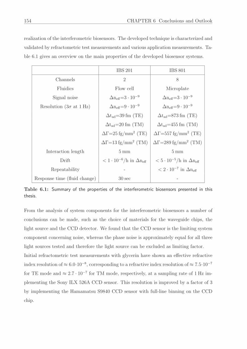
154 CHAPTER 6 Conclusions and Outlook
realization of the interferometric biosensors. The developed technique is characterized and
validated by refractometric test measurements and various application measurements. Ta-
ble 6.1 gives an overview on the main properties of the developed biosensor systems.
IBS 201 IBS 801
Channels 2 8
Fluidics Flow cell Microplate
Signal noise ∆neff=3 · 10−9 ∆neff=3 · 10−9
Resolution (3σ at 1 Hz) ∆neff=9 · 10−9 ∆neff=9 · 10−9
∆tad=39 fm (TE) ∆tad=873 fm (TE)
∆tad=20 fm (TM) ∆tad=455 fm (TM)
∆Γ=25 fg/mm2 (TE) ∆Γ=557 fg/mm2 (TE)
∆Γ=13 fg/mm2 (TM) ∆Γ=289 fg/mm2 (TM)
Interaction length 5 mm 5 mm
Drift < 1 · 10−6/h in ∆neff < 5 · 10−5/h in ∆neff
Repeatability - < 2 · 10−7 in ∆neff
Response time (fluid change) 30 sec -
Table 6.1: Summary of the properties of the interferometric biosensors presented in this
thesis.
From the analysis of system components for the interferometric biosensors a number of
conclusions can be made, such as the choice of materials for the waveguide chips, the
light source and the CCD detector. We found that the CCD sensor is the limiting system
component concerning noise, whereas the phase noise is approximately equal for all three
light sources tested and therefore the light source can be excluded as limiting factor.
Initial refractometric test measurements with glycerin have shown an effective refractive
index resolution of ≈ 6.0·10−8, corresponding to a refractive index resolution of ≈ 7.5·10−7
for TE mode and ≈ 2.7 · 10−7 for TM mode, respectively, at a sampling rate of 1 Hz im-
plementing the Sony ILX 526A CCD sensor. This resolution is improved by a factor of 3
by implementing the Hamamatsu S9840 CCD sensor with full-line binning on the CCD
chip.

6.1 Summary of the results 155
The experimentally derived sensitivity constants of the interferometer system are in very
good accordance with the theoretical values derived from waveguide theory. The flow-cell
system shows a good long-term stability with a typical drift of < 1 · 10−6/h in ∆neff .
We furthermore present the realized setup of the interferometric biosensor with an MTP-
formatted 8-well frame as fluidic element. This system is also characterized by refracto-
metric test measurements, including an evaluation of the experimental results compared to
theory and the results obtained with the flow cell system. Initial refractometric test mea-
surements with ethanol have shown an effective refractive index resolution of ≈ 1.0 ·10−7,
corresponding to a refractive index resolution of ≈ 1.2 ·10−6 for TE mode and ≈ 4.5 ·10−7
for TM mode, respectively, at a sampling rate of 1 Hz. It was also found that, apart from
the CCD sensor being the limiting system component concerning noise, the resolution of
the system is finally limited by the repeatability of the recorded data values. The experi-
mentally derived sensitivity constants of the MTP interferometer system are also in good
accordance with the theoretical values derived from waveguide theory. The system shows
a long-term stability with a typical drift of < 5 · 10−5/h in ∆neff and a repeatability of
< 2 · 10−7 in ∆neff .
It has been shown experimentally that the interferometric biosensor with the two-channel
flow cell as fluidic element can be used for application measurements when kinetic infor-
mation about the affinity system is desired, while the microplate system allows the parallel
detection of up to 96 analytes within one measurement. The flow-cell system has been
successfully used for the detection of two standard affinity systems, biotin-streptavidin
and protein G (protein A)-immunoglobulin G. Moreover, the detection of biotinylated cy-
tochrome c and the detection of a tagged protein by its corresponding antibody relevant
for protein purification analysis has been presented. A detailed analysis of the surface
chemistry resulted in the optimization of the silanization and further modification for
a stable and reproducible process needed for successful immobilization of biotinylated
reagents. Estimations on the detection limit in terms of analyte concentration based on
the results obtained by refractometric test measurements show that the developed inter-
ferometric biosensor can detect analyte concentrations in the low pM-range, even out of
a complex sample matrix without significant unspecific binding.
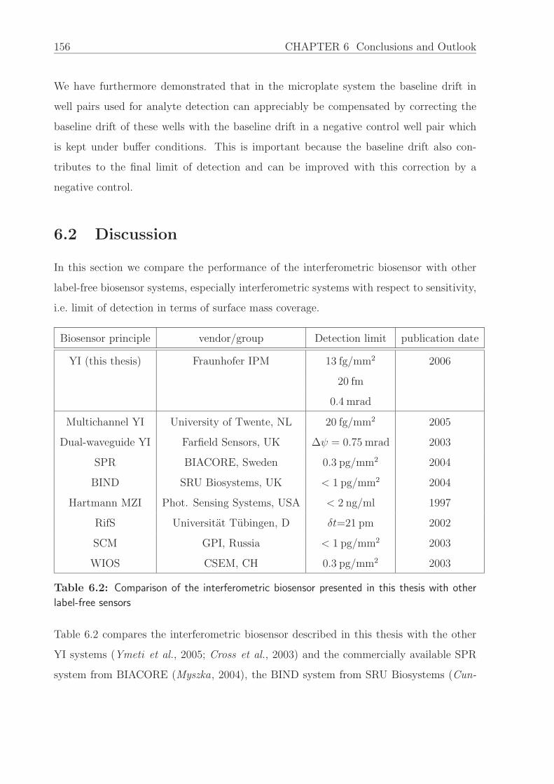
156 CHAPTER 6 Conclusions and Outlook
We have furthermore demonstrated that in the microplate system the baseline drift in
well pairs used for analyte detection can appreciably be compensated by correcting the
baseline drift of these wells with the baseline drift in a negative control well pair which
is kept under buffer conditions. This is important because the baseline drift also con-
tributes to the final limit of detection and can be improved with this correction by a
negative control.
6.2 Discussion
In this section we compare the performance of the interferometric biosensor with other
label-free biosensor systems, especially interferometric systems with respect to sensitivity,
i.e. limit of detection in terms of surface mass coverage.
Biosensor principle vendor/group Detection limit publication date
YI (this thesis) Fraunhofer IPM 13 fg/mm2 2006
20 fm
0.4 mrad
Multichannel YI University of Twente, NL 20 fg/mm2 2005
Dual-waveguide YI Farfield Sensors, UK ∆ψ = 0.75 mrad 2003
SPR BIACORE, Sweden 0.3 pg/mm2 2004
BIND SRU Biosystems, UK < 1 pg/mm2 2004
Hartmann MZI Phot. Sensing Systems, USA < 2 ng/ml 1997
RifS Universitat Tubingen, D δt=21 pm 2002
SCM GPI, Russia < 1 pg/mm2 2003
WIOS CSEM, CH 0.3 pg/mm2 2003
Table 6.2: Comparison of the interferometric biosensor presented in this thesis with other
label-free sensors
Table 6.2 compares the interferometric biosensor described in this thesis with the other
YI systems (Ymeti et al., 2005; Cross et al., 2003) and the commercially available SPR
system from BIACORE (Myszka, 2004), the BIND system from SRU Biosystems (Cun-

6.3 Outlook 157
ningham et al., 2004) and the MZI developed by Photonic Sensing Systems (Schneider
et al., 1997). Examples of other non-commercial systems are the RifS system (Kroger
et al., 2002), the SCM (Nikitin et al., 2003) and the WIOS system developed at the
CSEM (Cottier et al., 2003).
Compared to these other label-free techniques, the interferometric biosensor presented in
this thesis demonstrates a higher sensitivity in terms of refractive index and surface mass
coverage resolution. Furthermore our interferometric biosensor allows a configuration for
parallel detection of currently up to 96 analytes, compared to a maximum of four channels
implemented in other techniques.
Based on the application measurement results, it has been demonstrated that the interfer-
ometric biosensor can be used for various biological and biochemical applications in fields
like diagnostics, assay development or medical screening. The technique is characterized
by its very high sensitivity while allowing the parallel detection of up to 96 analytes. The
intrinsic reference compensates for temperature fluctuations in the ambient as well as pH
changes in the buffer. Effects caused by unspecific binding can also be reduced by simulta-
neously applying the same buffers or analyte solutions to the measurement and reference
channel. The established surface chemistry on the Ta2O5 waveguide chips allows a stable
and reproducible immobilization of commonly used biotinylated reagents.
Since the technology presented here does not rely on labeling of analytes, it saves several
time- and cost-consuming preparation steps necessary for label-based techniques such as
ELISA. It offers real-time monitoring of biomolecular binding events, allowing to evaluate
reaction kinetics and concentration determinations.
6.3 Outlook
In this section we want to present some aspects on further improvements and possible
application fields of the developed interferometric biosensor. The aforementioned appli-
cation measurements already showed the suitability of the biosensor system in fields like
immunoassay development, kinetic rate determination and secondary screening. Similarly
the detection of other immunoreactants, combined with the development of the appro-

158 CHAPTER 6 Conclusions and Outlook
priate surface chemistry, would be possible in research areas like medical screening or
diagnostics.
Currently waveguide chips fabricated on glass substrates are implemented into the in-
terferometric biosensor. These waveguide chips showed a very good batch-to-batch re-
producibility, as well as a homogeneous and reproducible waveguide layer. This high
waveguide chip quality ensures high quality measurements, yet also means a consider-
able cost per measurement. Especially for HTS applications, the cost of consumables
like sensor chips is an important issue. For this reason, sensor chips with polymers as
substrate instead of glass might contribute to a decrease of the costs for the waveguide
chips. First approaches of fabricating waveguide films on polymers have shown promising
results (Maisenholder , 2004), yet the reproducibility of the gratings and the waveguide
homogeneity still need improvements to reach the same quality than the glass substrate-
based sensor chips.
The developed biosensor system for microplate readout is currently designed to read a
single data point (two wells) at a time. For a higher parallelization and faster readout
the optical design of the system could be easily modified to read a complete row of an
MTP (8 wells) at a time, or even extended to read a 384 well MTP. Yet for a 384 well
MTP the interaction length of currently 5 mm would have to be decreased to ≈4.5 mm,
thereby sacrificing ≈10% of the currently achieved sensitivity, but reading 4 times more
data points. Here the main application focus would be primary screening, including new
compounds.
The results presented in this thesis show the suitability of the interferometric biosensor
as a higly sensitive sensing system for a wide variety of applications. These application
fields could be even extended by further improvements of the sensor system, providing a
label-free detection system as essential part in many different research areas.

Appendices
159


Appendix A: List of chemicals


Appendix B: Protocol for silanization procedure
Chemicals needed: Toluene (absolute), triethylamine, 3-glycidoxy-propyl-triethoxysilane
(GOPS)
• Chips have to be cleaned thoroughly before silanization!
• Put chips into the reaction vessels and plug them with stoppers.
• Start up manometer. Wait at least 2 minutes before the right atmospheric pressure
is displayed. If the atmospheric pressure value given deviates more than 100mbar,
the right value has to be reset manually.
• Start up vacuum pump.
• Put dewar filled with liquid nitrogen under cryo trap.
• Evacuate reaction vessels for approx. 10 minutes.
• Open main valve at the argon cylinder; first manometer shows pressure in the gas
cylinder.
• Open small valve (on the right side) and check bubble counter for reaction!
• Flood reaction vessels with argon; caution! Silicone from the bubble counter might
be dragged into the apparatus!
• Repeat evacuating and flooding of vessels at least once.
• Use remaining outlet for flooding of the toluene bottle with argon while taking 10ml
of toluene for each reaction vessel and dispensing it respectively.
• Dispense 28.8 µl of triethylamine and 28.8 µl of silane into each vessel accordingly.
• Close small valves at the reaction vessels.
• Close main valve at the argon cylinder. Wait until both manometers show zero.
• Close small valve at the cylinder.

• Shut down vacuum pump.
• Remove dewar, dispose of liquid nitrogen.
• Aerate whole apparatus with remaining outlet.
• Shut down manometer.
• Wait at least 16 hours, then remove chips from reaction vessels into a glass perti
dish and cure them at 120 Cfor 4 hours.
• Rinse with deionized water.
• Dry under liquid nitrogen or air.
• Clean reaction vessels with isopropanol and let dry.
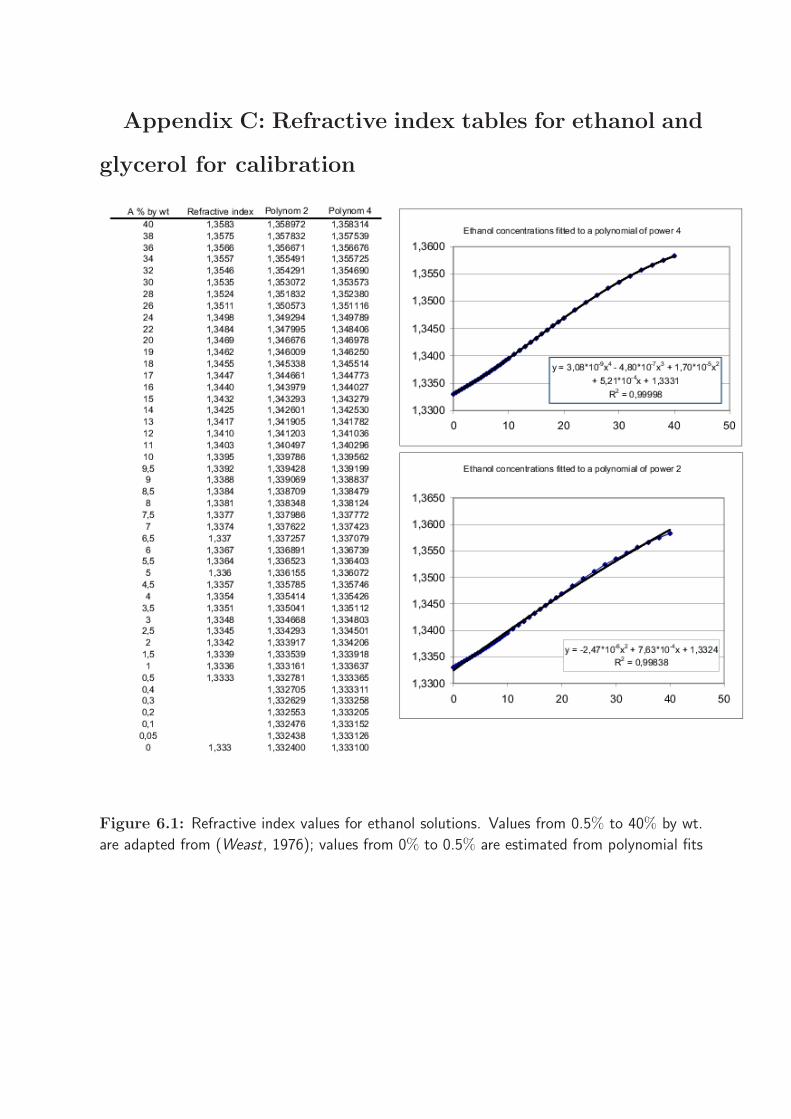
Appendix C: Refractive index tables for ethanol and
glycerol for calibration
Figure 6.1: Refractive index values for ethanol solutions. Values from 0.5% to 40% by wt.
are adapted from (Weast, 1976); values from 0% to 0.5% are estimated from polynomial fits

Figure 6.2: Refractive index values for glycerin solutions. Values from 0.5% to 40% by wt.
are adapted from (Weast, 1976); values from 0% to 0.5% are estimated from polynomial fits
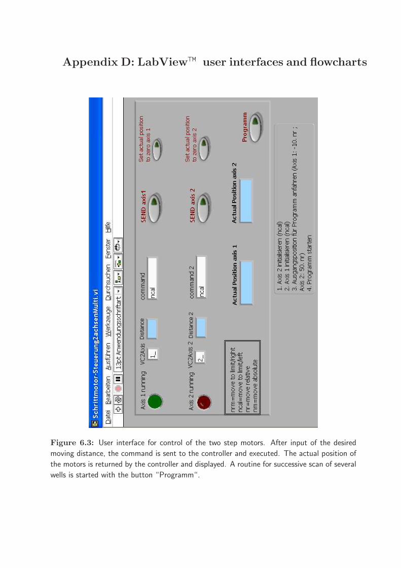
Appendix D: LabView™ user interfaces and flowcharts
Figure 6.3: User interface for control of the two step motors. After input of the desired
moving distance, the command is sent to the controller and executed. The actual position of
the motors is returned by the controller and displayed. A routine for successive scan of several
wells is started with the button “Programm“.
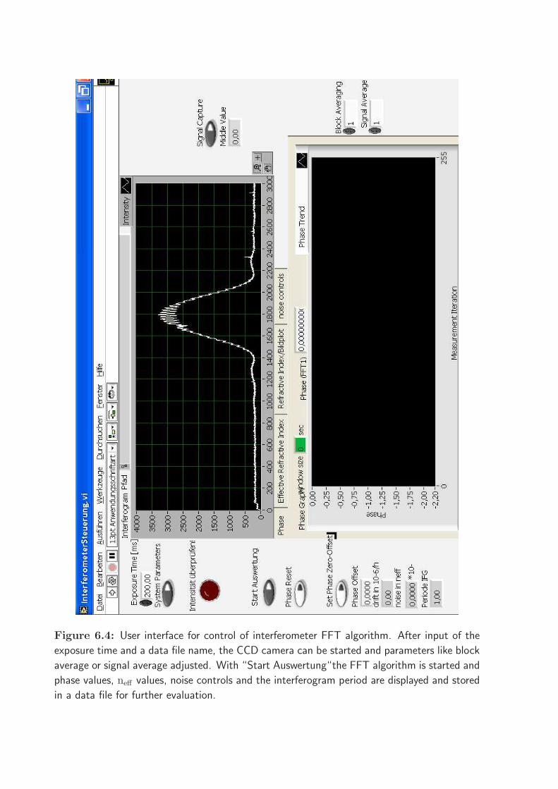
Figure 6.4: User interface for control of interferometer FFT algorithm. After input of the
exposure time and a data file name, the CCD camera can be started and parameters like block
average or signal average adjusted. With “Start Auswertung“the FFT algorithm is started and
phase values, neff values, noise controls and the interferogram period are displayed and stored
in a data file for further evaluation.

Figure 6.5: Flowchart FFT
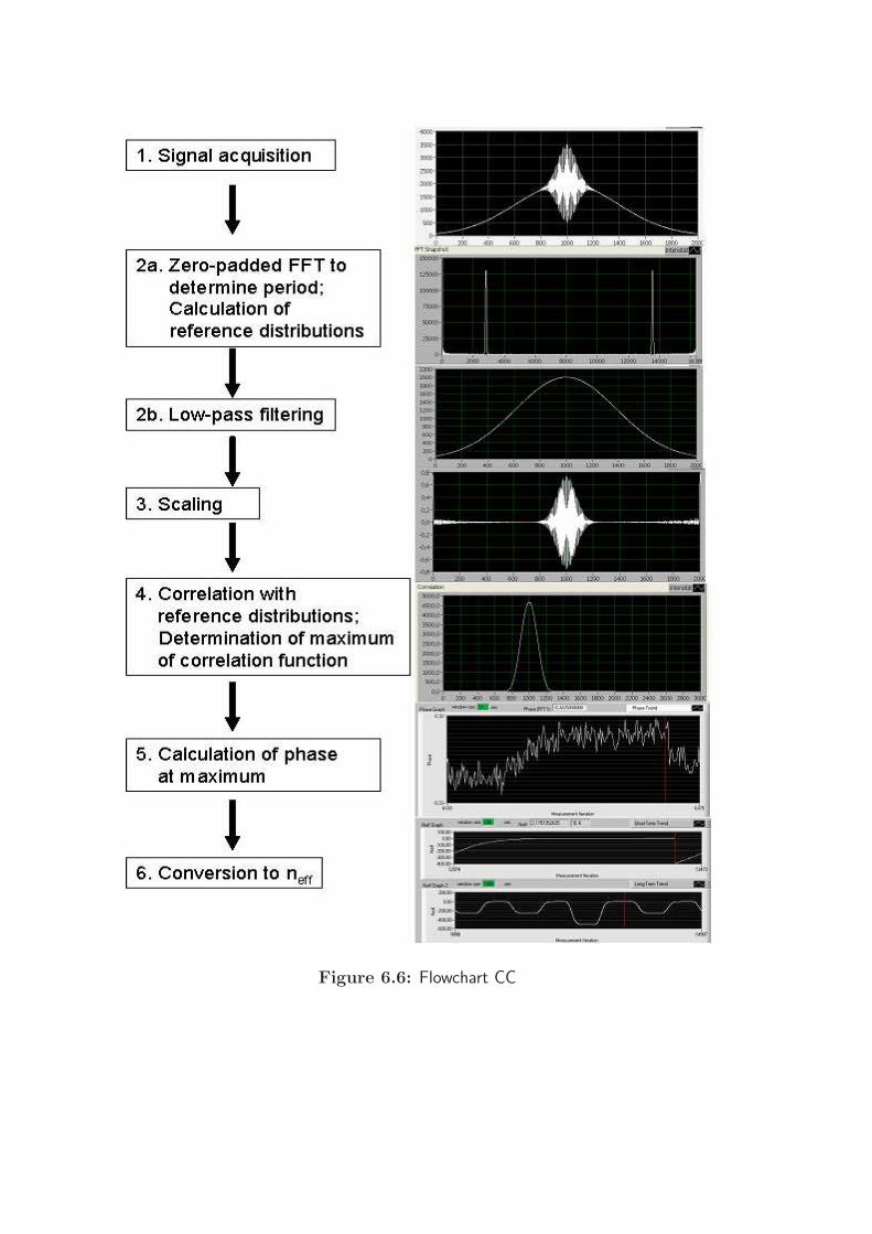
Figure 6.6: Flowchart CC
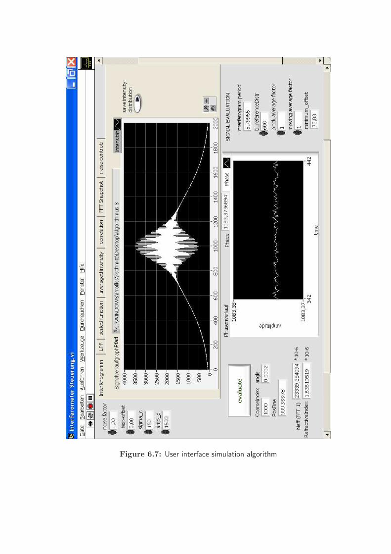
Figure 6.7: User interface simulation algorithm

/*Generation of test function*/
#include <stdio.h>
#include <stdlib.h>
#include <conio.h>
#include <math.h>
#include <time.h>
#include <sys/timeb.h>
#include <string.h>
#ifdef WIN32
# define DLLEXPORT __declspec(dllexport)
#else
# define DLLEXPORT
#endif
DLLEXPORT char Testfunktion_desc[] = "creates the testfunction for test purpose";
#define TWO_PI 6.28318530717959
static int counter=0;
static double indexshift=0;
static double randomarray [10000];
DLLEXPORT double Testfunktion (double *testfunktion, int arraysize,
double offset, double sigmac, double faktor, double ampc)
// Declarations
int i;
// Envelope function
double e; //function
double ampe = 2000; //amplitude of envelope function
double xe0 = 1000; //center pixel
double sigmae = 550; //fwhm in px
//Coherence function
double c; //function
double xc0 = 1000; //center pixel
double p=5.80; //period
for ( i=0; i < arraysize; i++ )
randomarray[i]=(rand()%10)*faktor; //adds noise, faktor variable
e = ampe * exp (-(i-xe0)*(i-xe0)/(sigmae*sigmae)); //envelope function
c = ampc * exp (-(i-xc0-indexshift)*(i-xc0-indexshift)/(sigmac*sigmac));
//coher. function
testfunktion[i] = e*(1+c/ampe * cos(TWO_PI*(i-xc-
0indexshift)/p))+offset+randomarray[i];
counter++; // increase loop counter
indexshift+=0.05; //simulation of phase shift
return 1;
Figure 6.8: DLL for generation of test function


Bibliography
Adam, G., P. Lauger and G. Stark, Physikalische Chemie und Biophysik, Springer Verlag,
1995
Baird, C. and D. Myszka, Current and emerging commercial optical biosensors, Journal
of Molecular Recognition, Vol. 14 pp 261–268, 2001
Baker, K., M. Rendall, A. Patel, P. Boyd, M. Hoare, R. Freedman and D. James, Rapid
monitoring of recombinant protein products: a comparison of current technologies,
Trends in Biotechnology , Vol. 20 pp 149–156, 2002
Bilitewski, U., F. Bier and A. Brandenburg, Immunobiosensors based on grating cou-
plers, in Rogers, K. R. and A. Mulchandani (Eds.), Affinity biosensors - techniques and
protocols, Vol. 12, pp 121–134, Humana Press, 1998
Bjorck, L. and G. Kronwall, Purification and some properties of streptococcal protein G,
a novel IgG-binding reagent, J. Immunol., Vol. 133 pp 969–974, 1984
Blake, R., Cellular screening assays using fluorescence microscopy, Current Opinion in
Pharmacology , Vol. 1 pp 533–539, 2001
Born, M. and E. Wolf, Principles of Optics, 7th ed., Cambridge University Press, 1999
Brandenburg, A., Differential refractometry by an integrated -optical Young interferom-
eter, Sensors and Actuators B , Vol. 38-39 pp 266–271, 1997
Brandenburg, A., R. Krauter, C. Kunzel, M. Stefan and H. Schulte, Interferometric sensor
for detection of surface-bound bioreactions, Applied Optics , Vol. 39 pp 6396–6405, 2000
175

176 BIBLIOGRAPHY
Busse, S., V. Scheumann, B. Menges and S. Mittler, Sensitivity studies for specific binding
reactions using the biotin/SAv system by evanescent optical methods, Biosensors &
Bioelectronics , 2002
Cammann, K., Biosensoren, in: Instrumentelle Ananlytische Chemie, Spektrum
Akademischer Verlag, Weinheim, pp 52–79, 2000
Chen, K., C. Hsu and D.-C. Su, Interferometric optical sensor for measuring glucose
concentration, Applied Optics , Vol. 42 pp 5774–5776, 2003
Cooper, M., Optical biosensors in drug discovery, Nature reviews, Vol. 1 pp 515–528,
2002
Cooper, M., Label-free screening of bio-molecular interactions, Analytical and Bioanalyt-
ical Chemistry , Vol. 377 pp 834–842, 2003
Cottier, K., M. Wiki, G. Voirin, H. Gao and R. Kunz, Label-free highly sensitive detection
of (small) molecules by wavelength interrogation of integrated optical chips, Sensors and
Actuators B , Vol. 91 pp 241–251, 2003
Cross, G., A. Reeves, S. Brand, J. Popplewell, L. Peel, M. Swann and N. Freeman, A new
quantitative optical biosensor for protein characterization, Biosensors & Bioelectronics ,
Vol. 19 pp 383–390, 2003
Cunningham, B., P. Li, S. Schulz, B. Lin, C. Baird, J. Gerstenmaier, C. Genick, F. Wang,
E. Fine and L. Laing, Label-free assays on the BIND system, Journal of Biomolecular
Screening , Vol. 9 pp 481–490, 2004
Cunningham, B., B. Lin, J. Qiu, P. Li, J. Pepper and B. Hugh, A plastic colorimetric reso-
nant optical biosensor for multiparallel detection of label-free biochemical interactions,
Sensors and Actuators B , Vol. 85 pp 219–226, 2002
Davies, C., Introduction to immunoassay principles, in Wild, D. (Ed.), The immunoassay
handbook, Nature publishing group, 2001
BIBLIOGRAPHY 177
de Feijter, J. A., J. Benjamins and F. A. Veer, Ellipsometry as a tool to study the adsorp-
tion behaviour of synthetic and biolpolymers at the air-water interface, Biopolymers ,
Vol. 17 pp 1759–1772, 1978
Elender, G., M. Kuhner and E. Sackmann, Functionalisation of Si/SiO2 and glass surfaces
with ultrathin dextran films and deposition of liquid bilayers, Biosensors & Bioelectron-
ics , Vol. 11 pp 565–577, 1996
Fox, P., R. Scholten, M. Walkiewicz and R. Drullinger, A reliable, compact, low-cost
Michelson wavemeter for laser wavelength measurement, American Journal of Physics ,
Vol. 67 pp 624–630, 1999
Goodman, J., Introduction to Fourier Optics, McGraw-Hill, 1988
Hartmann, S., Personal communication, 2005
Hebestreit, H., Proteomics: an holistic analysis of nature’s proteins, Current Opinion in
Pharmacology , Vol. 1 pp 513–520, 2001
Hecht, E., Optik, Oldenbourg Verlag, 2001
Hendrickson, W., A. Pahler, J. Smith, Y. Satow, E. Merritt and R. Phizackerley, Crystal
structure of core streptavidin determined from multi-wavelength anomalous diffraction
of synchrotron radiation, Proc. Natl. Acad. Sci., Vol. 86 pp 2190–2194, 1989
Hermanson, G. T., A. K. Mallia and P. K. Smith, Immobilized affinity ligand techniques,
Academic Press N.Y., 1992
Hertzberg, R. P. and A. J. Pope, High-throughput screening: new technology for the 21st
century, Current Opinion in Chemical Biology , Vol. 4 pp 445–451, 2000
Hoffmann, C., Selbstorganisierende Organosilansysteme zur Funktionalisierung oxidischer
Siliziumoberflachen fur die gerichtete Peptid- und Proteinimmobilisierung, 2002
Karlsson, R. and S. Lofas, Kinetic analysis of the interaction between an analyte in
solution and an immobilized protein, in Cass, T. and F. Ligler (Eds.), Immobilized

178 BIBLIOGRAPHY
Biomolecules in Analysis-a practical approach, pp 149–165, Oxford University Press,
1998
Kogelnik, H., Theory of Optical Waveguides, in Tamir, T. (Ed.), Guided-Wave Optoelec-
tronics, pp 7–87, Springer Verlag, 1988
Kretschmann, E. and H. Raether, Radiative decay of non radiative surface plasmons
excited by light, Zeitschrift fuer Naturforschung , Vol. 23A pp 2135–2136, 1968
Kroger, K., J. Bauer, B. Fleckenstein, J. Rademann, G. Jung and G. Gauglitz, Epitope-
mapping of transglutaminase with parallel label-free optical detection, Biosensors &
Bioelectronics , Vol. 17 pp 937–944, 2002
Kuhlke, D., Optik - Grundlagen und Anwendungen, Verlag Harri Deutsch, 2004
Kujawinska, M. and J. Wojciak, High accuracy Fourier transform fringe pattern analysis,
Optics and Lasers in Engineering , Vol. 14 pp 325–339, 1991
Lane, H. D., Antibodies: a laboratory manual, Cold Spring Harbor Laboratory Press
N.Y., 1998
Lang, C. and N. Pucker, Mathematische Methoden in der Physik, Spektrum Akademischer
Verlag Berlin, 1998
Laureyn, W., F. Frederix, A. Campitelli, J. J. Pireaux and G. Maes, The silanization
of tantalum pentoxide for biosensor realization, Poster presentation, source: internet ,
2001
Le Grange, J. D. and J. L. Markham, Effects of surface hydration on the deposition of
silane monolayers on silica, Langmuir , Vol. 9 pp 1749–1753, 1993
Leatherbarrow, R. J. and P. R. Edwards, Analysis of molecular recognition using optical
biosensors, Current Opinion in Chemical Biology , Vol. 3 pp 544–547, 1999
Lehninger, A., D. Nelson and M. Cox, Prinzipien der Biochemie, Spektrum Akademischer
Verlag, 1994
BIBLIOGRAPHY 179
Lindner, H., H. Brauer and C. Lehmann, Taschenbuch der Elektrotechnik und Elektronik,
Fachbuchverlag Leipzig, 1999
Lottspeich, F. and H. Zorbas, Bioanalytik, Spektrum Akademischer Verlag, 1998
Lukosz, W., Principles and sensitivities of integrated optical and surface plasmon sensors
for direct affinity sensing and immunosensing, Biosensors & Bioelectronics , Vol. 6 pp
215–225, 1991
Lukosz, W., D. Clerc, P. Nellen, C. Stamm and P. Weiss, Output grating couplers on
planar optical waveguides as direct immunosensors, Biosensors & Bioelectronics , Vol. 6
pp 227–232, 1991
MacKenzie, R., Development of an interferometric biosensor, 2003
Maisenholder, B., Personal communication, 2004
Meyer, M., Signalverarbeitung, Vieweg Verlag, 2003
Morgan, H. and D. Taylor, A surface plasmon resonance immunosensor based on the
streptavidin-biotin complex, Biosensors & Bioelectronics , Vol. 7 pp 405–410, 1992
Myszka, D., Improving biosensor analysis, Journal of Molecular Recognition, Vol. 12 pp
279–284, 1999
Myszka, D., Analysis of small-molecule interactions using BiacoreS51 technology, Analyt-
ical Biochemistry , Vol. 329 pp 316–323, 2004
Myszka, D., X. He, M. Dembo, T. Morton and B. Goldstein, Extending the range of
rate constants available from BIACORE: interpreting mass transport-influenced binding
data, Biophysical Journal , Vol. 75 pp 583–594, 1998
Nakadate, S., Phase detection of equidistant fringes for highly sensitive optical sensing.
I. Principle and error analyses, Journal of the Optical Society of America A, Vol. 5 pp
1258–1264, 1988
180 BIBLIOGRAPHY
Nieba, L., A. Krebber and A. Plckthun, Competition BIACORE for measuring true
affinities: large differences from values determined from binding kinetics, Analytical
Biochemistry , Vol. 234 pp 155–165, 1996
Nikitin, P. I., M. V. Valeiko and B. G. Gorshkov, New direct optical biosensors for multi-
analyte detection, Sensors and Actuators B , Vol. 90 pp 46–51, 2003
Pierce, http://www.piercenet.com, 2005
Polzius, R., E. Dießel, F. Bier and U. Bilitewski, Real-time observation of affinity reactions
using grating couplers: determination of the detection limit and calculation of kinetic
rate constants, Analytical Biochemistry , Vol. 248 pp 269–276, 1997
Polzius, R., T. Schneider, F. Bier and U. Bilitewski, Optimization of biosensing using
grating couplers: immobilization on tantalum oxide waveguides, Biosensors & Bioelec-
tronics , Vol. 11 pp 503–514, 1996
Prime, K. and G. Whitesides, Self-assembled organic monolayers: model systems for
studying adsorption of proteins at surfaces, Science, Vol. 252 pp 1164–1167, 1991
Prime, K. and G. Whitesides, Adsorption of proteins onto surfaces containing end-
attached oligo(ethylene oxide): a model system using self-assembled monolayers, J.
Am. Chem. Soc., Vol. 115 pp 10714–10721, 1993
Ramsden, J., Optical biosensors, Journal of Molecular Recognition, Vol. 10 pp 109–120,
1997
Saha, K., F. Bender and E. Gizeli, Comparative study of IgG binding to proteins G
and A: nonequilibrium kinetic and binding constant determination with the acoustic
waveguide device, Analytical Chemistry , Vol. 75 pp 835–842, 2003
Saleh, B. and M. Teich, Fundamentals of Photonics, Addison-Wesley, 1990
Savage, M. D., Avidin-Biotin Chemistry: A handbook, Pierce Chemical Co, 1992
Sayle, R., http://www.umass.edu/microbio/rasmol/, 1993
BIBLIOGRAPHY 181
Schneider, B., E. L. Dickinson, M. D. Vach, J. V. Hoijer and L. V. Howard, Highly sensitive
optical chip immunoassays in human serum, Biosensors & Bioelectronics , Vol. 15 pp
13–20, 2000
Schneider, B., J. Edwards and N. Hartman, Hartman interferometer: versatile inte-
grated optic sensor for label-free, real-time quantification of nucleic acids, proteins,
and pathogens, Clinical Chemistry , Vol. 43 pp 1757–1763, 1997
Schrufer, E., Signalverarbeitung: Numerische Verarbeitung digitaler Signale, 2nd ed.,
Hanser Verlag, 1992
Schutz, A., Einsatz der reflektometrischen Interferenzspektroskopie (RIfS) zur
markierungsfreien Affinitatsdetektion fur das Hochdurchsatzscreening, Dissertation,
Universitat Tubingen, 2000
Sober, H., Handbook of Biochemistry 2nd ed., Chemical Rubber Co., Cleveland, Ohio,
1970
Stamm, C., R. Dangel and W. Lukosz, Biosensing with the integrated-optical difference
interferometer: dual-wavelength operation, Optics Communications , Vol. 153 pp 347–
359, 1998
Stevens, R., Design of high-throughput methods of protein production for structural bi-
ology, Structure, Vol. 8 pp R177–R185, 2000
Superlum, Superluminescent Diode Modules-General Operation Instructions, Superlum
Moscow, 2003
Surolia, A., D. Pain and M. I. Khan, Protein A: nature’s universal anti-antibody - a
review on properties and applications of protein A, Trends Biochem. Sci., Vol. 7 pp
74–76, 1982
Tiefenthaler, K. and W. Lukosz, Sensitivity of grating couplers as integrated-optical chem-
ical sensors, Journal of the Optical Society of America B , Vol. 6 pp 209–220, 1989

182 BIBLIOGRAPHY
Tovar, G., Funktionalisierung und Strukturierung von oxidischen Oberflachen mit biolo-
gischen und synthetischen Polymeren, 1995
Tsukruk, V., I. Luzinov and D. Julthongpiput, Sticky molecular surfaces: epoxysilane
self-assembled monolayers, Langmuir , Vol. 15 pp 3029–3032, 1999
van der Merwe, P., Surface plasmon resonance, source: internet , pp 1–50, 2005
Weast, R., Handbook of Physics and Chemistry, CRC Press, 1976
Weber, P., D. H. Ohlendorf, J. J. Wendoloski and F. R. Salemme, Structural origins of
high-affinity biotin binding to streptavidin, Science, Vol. 247 pp 85–88, 1989
Weisser, M., G. Tovar, S. Mittler, W. Knoll, F. Brosinger, H. Freimuth, M. Lacher
and W. Ehrfeld, Specific bio-recognition reactions observed with an integrated Mach-
Zehnder interferometer, Biosensors & Bioelectronics , Vol. 14 pp 405–411, 1999
www.biacore.com, Surface plasmon resonance, 2003
www.invitrogen.com, AlexaFluor647 information, 2005
Ymeti, A., J. Kanger, J. Greve, G. A. J. Besselink, P. Lambeck, R. Wijn and R. Heideman,
Integration of microfluidics with a four-channel integrated optical Young interferometer
immunosensor, Biosensors & Bioelectronics , Vol. 20 pp 1417–1421, 2005
Ymeti, A., J. Kanger, R. Wijn, P. Lambeck and J. Greve, Development of a multichannel
integrated interferometer immunosensor, Sensors and Actuators B , Vol. 83 pp 1–7,
2002
Publications
• K. Schmitt, B. Schirmer, C. Hoffmann, A. Brandenburg, P. Meyrueis (2006)
Interferometric biosensor based on planar optical waveguide sensor chips for label-
free detection of surface bound bioreactions, in preparation
• C. Hoffmann, K. Schmitt, B. Schirmer, S. Hartmann (2006)
Rapid protein expression analysis with an interferometric biosensor in laboratory
environment, in preparation
• K. Schmitt, B. Schirmer, A. Brandenburg (2005)
Label-free detection of biomolecules by waveguide interferometry
Proc. SPIE Vol. 5855, p. 459-462
• K. Schmitt, B. Schirmer, C. Hoffmann, A. Brandenburg (2005)
Interferometer for label-free detection of biomolecules in MTP format
Poster presentation, SBS 11th Annual Conference and Exhibition, Sep 11-15, Geneva
• K. Schmitt, C. Hoffmann (2005)
Interferometrisches Messsystem zur markierungsfreien Analyse von biomolekularen
Bindungsreaktionen, in Aktuelle Wochenschau der GDCh, 44
• K. Schmitt, B. Schirmer, A. Brandenburg (2005)
Development of a label-free interferometric read-out system in MTP format
Presentation, 4. Deutsches Biosensor Symposium, Mar 13-16, Regensburg
• K. Schmitt, B. Schirmer, A. Brandenburg (2004)
Development of a highly sensitive interferometric biosensor
Proc. SPIE Vol. 5461, p. 22-29
183


Vita
Name: Katrin Schmitt
Date of birth: 22.08.1979
Place of birth: Emmendingen
Education:
2006: PhD thesis supervisor: Prof. Patrick Meyrueis
Title: A new waveguide interferometer for the label-free
detection of biomolecules
2003-2006 PhD at the Universite Louis Pasteur Strasbourg
carried out at the Fraunhofer IPM in Freiburg
2003: Master of Arts
Master thesis supervisor: Prof. Mark Raizen
Title: Optical neuronal guiding on the hypothalamic GnRH cell line GT1
2002-2003 Study of physics at the University of Texas at Austin
2001: Vordiplom
1999-2002 Study of physics at the Bayerische Julius-Maximilians-
Universitat Wurzburg
1999: Abitur
1992-1999 Dietrich-Bonhoeffer-Gymnasium Wertheim a. Main
1990-1992 Gymnasium Kenzingen
185


Resume: Le travail presente dans cette these decrit le developpement d’un nouveau dis-positif interferometrique pour la detection des interactions biomoleculaires sans adjuvant.Ce capteur par onde evanescente detecte des especes adsorbees car la masse a la surfacechange, base sur le principe optique d’un interferometre de Young. Nous introduisonsla base theoriques concernant l’architecture du systeme interferometrique et presentonsl’assemblage realise et bien dans une configuration a debit a deux canaux d’ecoulementet bien dans un systeme statique de micro plate. Le biocapteur realise est optimiseet caracterise par des tests refractometriques ainsi que valide a l’echelle experimentaleen l’appliquant a l’examen de differents reactions immunitaires. Les resultats de cetteapplication prouvent l’aptitude de ce biocapteur a haute sensibilite pour applicationssans adjuvant dans le spectre du diagnostic, du criblage et du developpement de testsd’immunite.
Title: A new waveguide interferometer for the label-free detection of biomolecules
Abstract: The work presented in this thesis describes the development of a new wave-guide interferometer for the label-free detection of biomolecular interactions. This evanes-cent field sensor detects changes in surface mass coverage on the waveguide sensor chip ina setup based on the optical principle of a Young interferometer. We introduce the the-oretical basis for the design of the interferometer system and present the realized designin both a two-channel flow-cell configuration and a microplate reading format. The re-alized biosensor is optimized and characterized by refractometric test measurements andexperimentally validated by application measurements on different immunoreactions. Theapplication measurement results show the suitability of this highly sensitive biosensor forlabel-free applications in fields like diagnostics, screening and immunoassay development.
Discipline: Physique et Photonique
Mots-Cles: Capteur interferometrique, detection sans adjuvant, champ evanescent, Ta2O5
guide d’ondeKeywords: interferometric sensor, label-free detection, evanescent field, Ta2O5 wave-guide
INTITULE ET ADRESSE DE L’U.F.R. ET DU LABORATOIRE:Ecole Nationale Superieure de Physique de StrasbourgLaboratoire des Systemes PhotoniquesParc d’Innovation, Pole API, Boulevard Sebastien Brant, 67400 ILLKIRCH - FranceTelephone: +33 (0) 390 244616Fax: +33 (0) 390 244619
Fraunhofer Institut fur Physikalische Messtechnik IPMHeidenhofstr. 879110 Freiburg - AllemagneTelephone: +49 (0) 761 88570Fax: +49 (0) 761 8857224


