
Large-Scale Data Processing with MapReduce
AAAI 2011 Tutorial
Jimmy LinUniversity of Maryland
Sunday, August 7, 2011
This work is licensed under a Creative Commons Attribution-Noncommercial-Share Alike 3.0 United StatesSee http://creativecommons.org/licenses/by-nc-sa/3.0/us/ for details
These slides are available on my homepage at http://www.umiacs.umd.edu/~jimmylin/

First things first… About me
Course history
Audience survey
Agenda Setting the stage: Why large data? Why is this different?
Introduction to MapReduce
MapReduce algorithm design
Text retrieval
Managing relational data
Graph algorithms
Beyond MapReduce

Expectations Focus on “thinking at scale”
Deconstruction into “design patterns”
Basic intuitions, not fancy math
Mapping well-known algorithms to MapReduce
Not a tutorial on programming Hadoop
Entry point to book

Setting the Stage:
Why large data?
Setting the stageIntroduction to MapReduceMapReduce algorithm designText retrievalManaging relational dataGraph algorithmsBeyond MapReduce

Source: Wikipedia (Everest)

How much data?
6.5 PB of user data + 50 TB/day (5/2009)
processes 20 PB a day (2008)
36 PB of user data + 80-90 TB/day (6/2010)
Wayback Machine: 3 PB + 100 TB/month (3/2009)
LHC: 15 PB a year(any day now)
LSST: 6-10 PB a year (~2015)
640K ought to be enough for anybody.
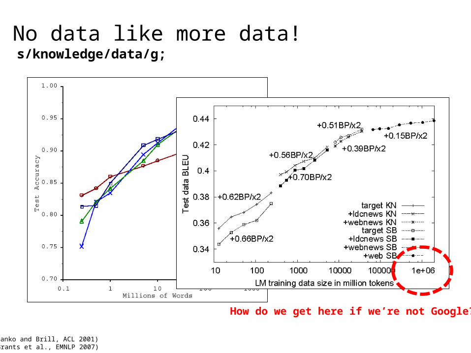
No data like more data!
(Banko and Brill, ACL 2001)(Brants et al., EMNLP 2007)
s/knowledge/data/g;
How do we get here if we’re not Google?

+ simple, distributed programming models cheap commodity clusters
= data-intensive computing for the masses!

Setting the Stage:
Why is this different?
Setting the stageIntroduction to MapReduceMapReduce algorithm designText retrievalManaging relational dataGraph algorithmsBeyond MapReduce
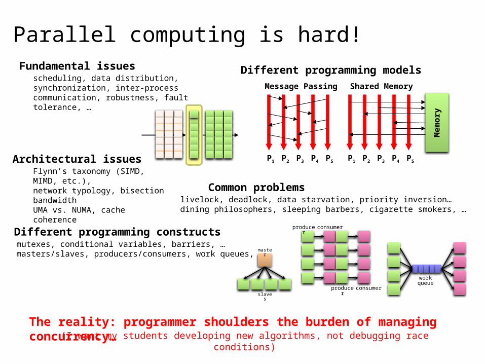
Parallel computing is hard!
Message Passing
P1 P2 P3 P4 P5
Shared Memory
P1 P2 P3 P4 P5
Me
mo
ry
Different programming models
Different programming constructsmutexes, conditional variables, barriers, …masters/slaves, producers/consumers, work queues, …
Fundamental issuesscheduling, data distribution, synchronization, inter-process communication, robustness, fault tolerance, …
Common problemslivelock, deadlock, data starvation, priority inversion…dining philosophers, sleeping barbers, cigarette smokers, …
Architectural issuesFlynn’s taxonomy (SIMD, MIMD, etc.),network typology, bisection bandwidthUMA vs. NUMA, cache coherence
The reality: programmer shoulders the burden of managing concurrency…(I want my students developing new algorithms, not debugging race conditions)
master
slaves
producer consumer
producer consumer
work queue

Where the rubber meets the road Concurrency is difficult to reason about
At the scale of datacenters (even across datacenters) In the presence of failures In terms of multiple interacting services
The reality: Lots of one-off solutions, custom code Write you own dedicated library, then program with it Burden on the programmer to explicitly manage everything

Source: Ricardo Guimarães Herrmann

Source: NY Times (6/14/2006)
The datacenter is the computer!
I think there is a world market for about five computers.
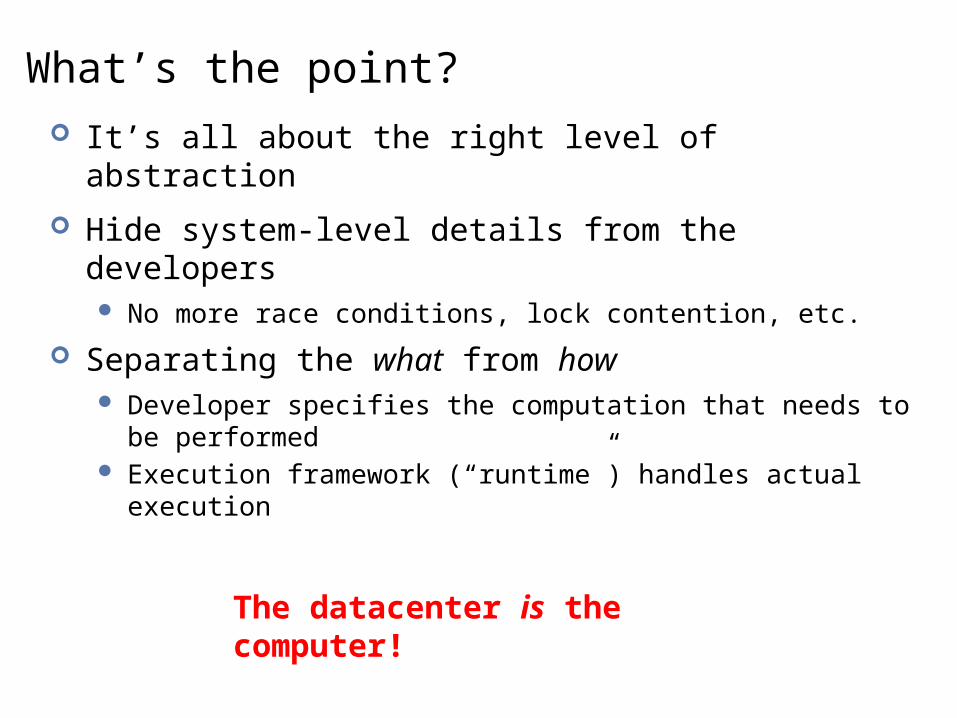
What’s the point? It’s all about the right level of abstraction
Hide system-level details from the developers No more race conditions, lock contention, etc.
Separating the what from how Developer specifies the computation that needs to be performed Execution framework (“runtime”) handles actual execution
The datacenter is the computer!
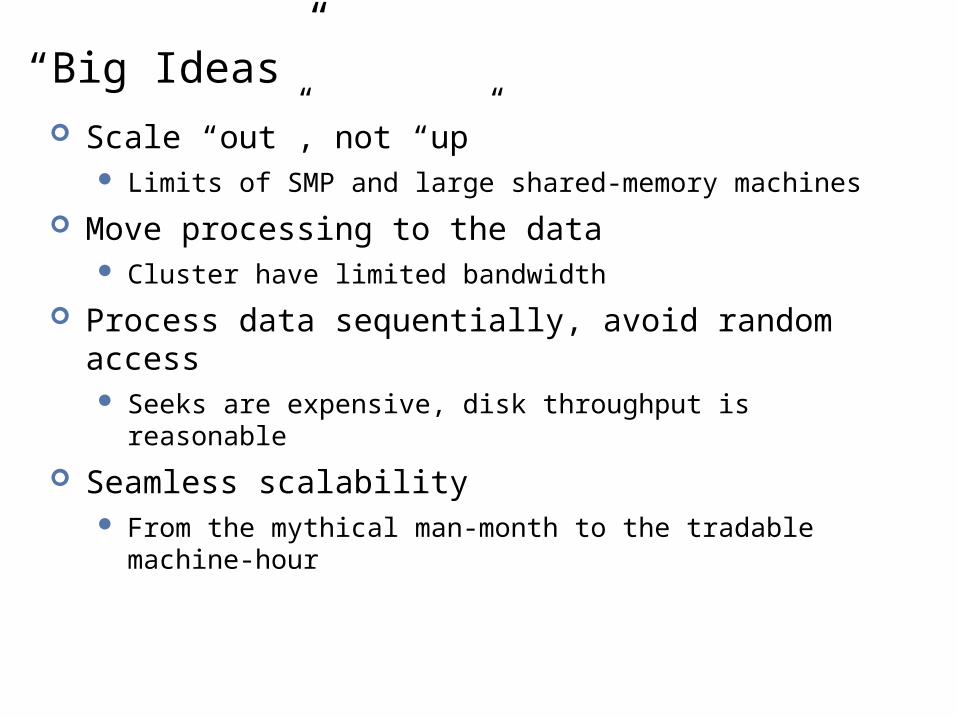
“Big Ideas” Scale “out”, not “up”
Limits of SMP and large shared-memory machines
Move processing to the data Cluster have limited bandwidth
Process data sequentially, avoid random access Seeks are expensive, disk throughput is reasonable
Seamless scalability From the mythical man-month to the tradable machine-hour
Introduction to MapReduce
Setting the stageIntroduction to MapReduceMapReduce algorithm designText retrievalManaging relational dataGraph algorithmsBeyond MapReduce
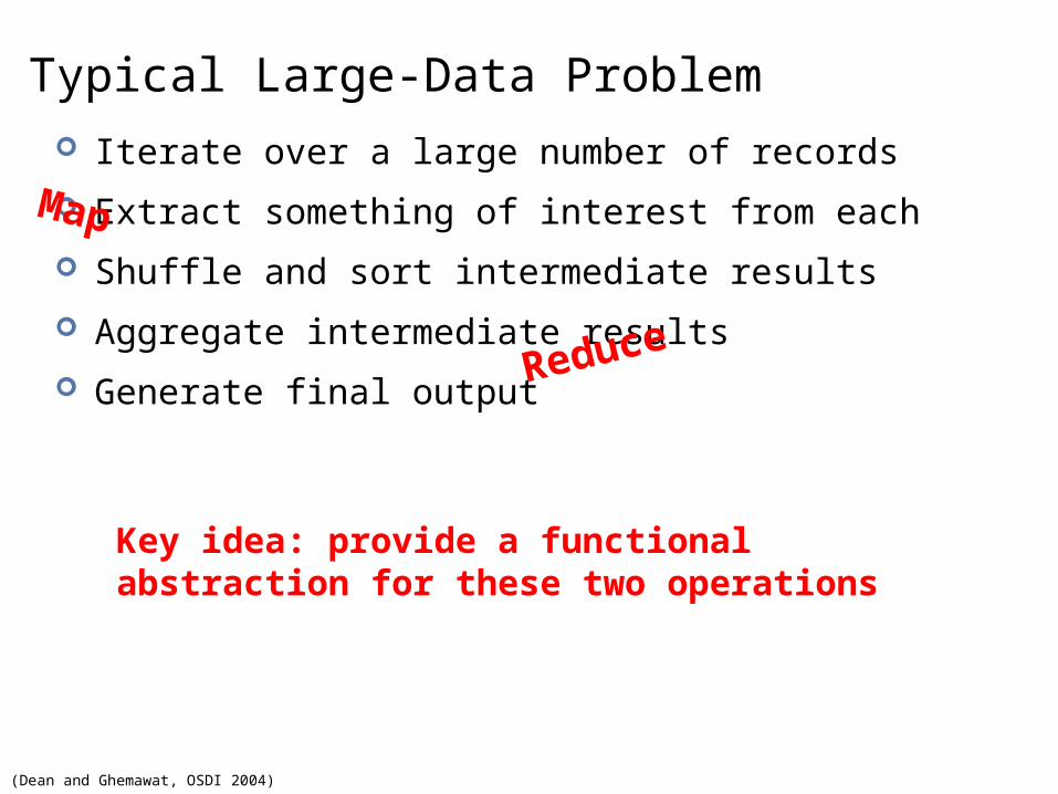
Typical Large-Data Problem Iterate over a large number of records
Extract something of interest from each
Shuffle and sort intermediate results
Aggregate intermediate results
Generate final output
Key idea: provide a functional abstraction for these two operations
Map
Reduce
(Dean and Ghemawat, OSDI 2004)
g g g g g
f f f f fMap
Fold
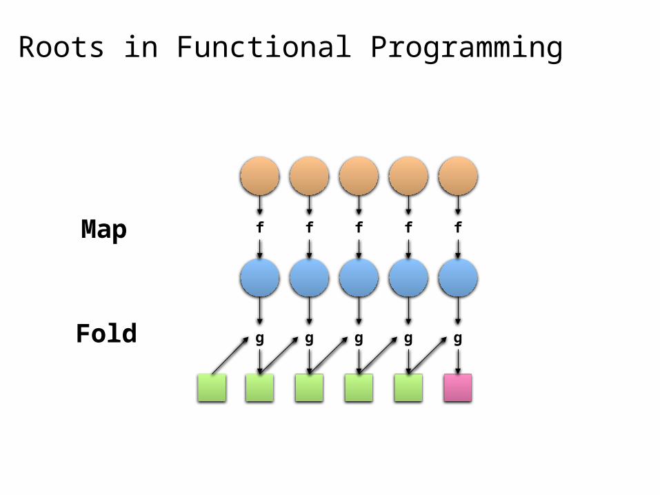
Roots in Functional Programming
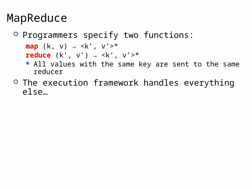
MapReduce Programmers specify two functions:
map (k, v) → <k’, v’>*reduce (k’, v’) → <k’, v’>* All values with the same key are sent to the same reducer
The execution framework handles everything else…
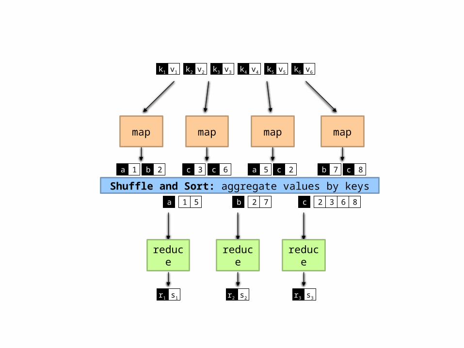
mapmap map map
Shuffle and Sort: aggregate values by keys
reduce reduce reduce
k1 k2 k3 k4 k5 k6v1 v2 v3 v4 v5 v6
ba 1 2 c c3 6 a c5 2 b c7 8
a 1 5 b 2 7 c 2 3 6 8
r1 s1 r2 s2 r3 s3
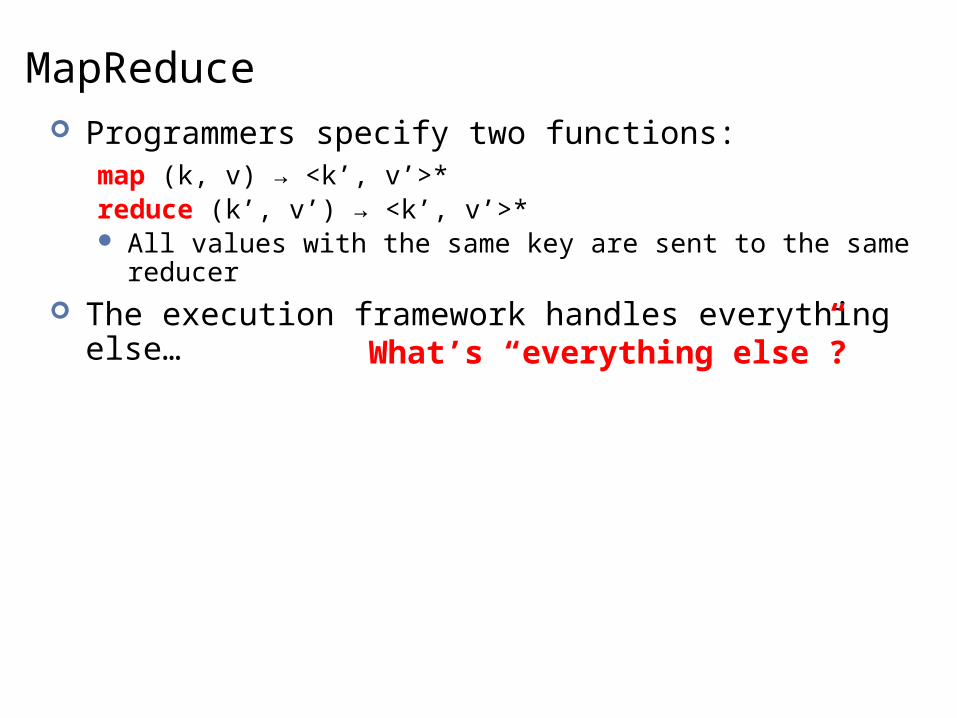
MapReduce Programmers specify two functions:
map (k, v) → <k’, v’>*reduce (k’, v’) → <k’, v’>* All values with the same key are sent to the same reducer
The execution framework handles everything else…
What’s “everything else”?
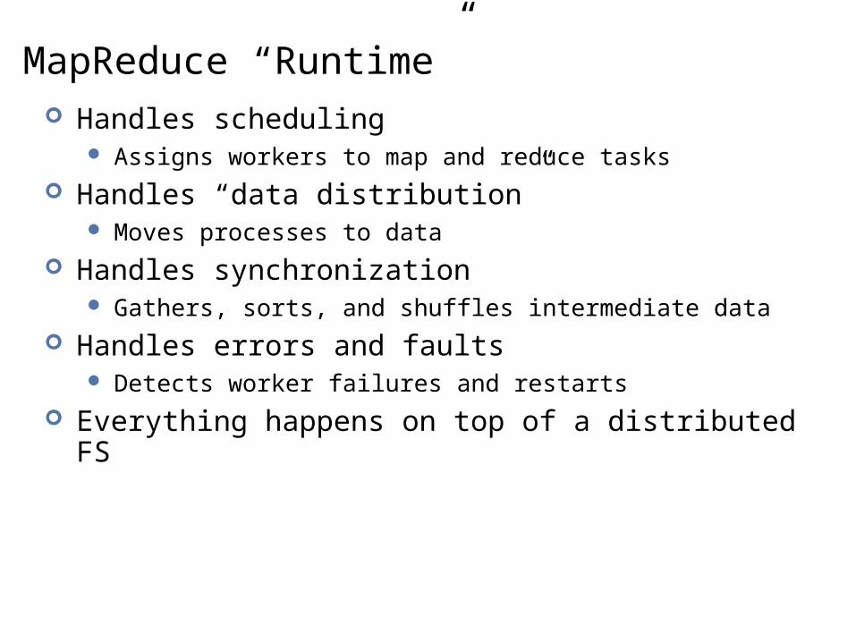
MapReduce “Runtime” Handles scheduling
Assigns workers to map and reduce tasks
Handles “data distribution” Moves processes to data
Handles synchronization Gathers, sorts, and shuffles intermediate data
Handles errors and faults Detects worker failures and restarts
Everything happens on top of a distributed FS
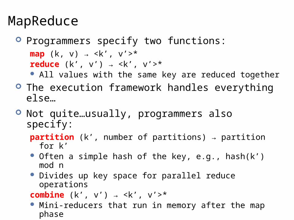
MapReduce Programmers specify two functions:
map (k, v) → <k’, v’>*reduce (k’, v’) → <k’, v’>* All values with the same key are reduced together
The execution framework handles everything else… Not quite…usually, programmers also specify:
partition (k’, number of partitions) → partition for k’ Often a simple hash of the key, e.g., hash(k’) mod n Divides up key space for parallel reduce operationscombine (k’, v’) → <k’, v’>* Mini-reducers that run in memory after the map phase Used as an optimization to reduce network traffic

combinecombine combine combine
ba 1 2 c 9 a c5 2 b c7 8
partition partition partition partition
mapmap map map
k1 k2 k3 k4 k5 k6v1 v2 v3 v4 v5 v6
ba 1 2 c c3 6 a c5 2 b c7 8
Shuffle and Sort: aggregate values by keys
reduce reduce reduce
a 1 5 b 2 7 c 2 9 8
r1 s1 r2 s2 r3 s3
c 2 3 6 8
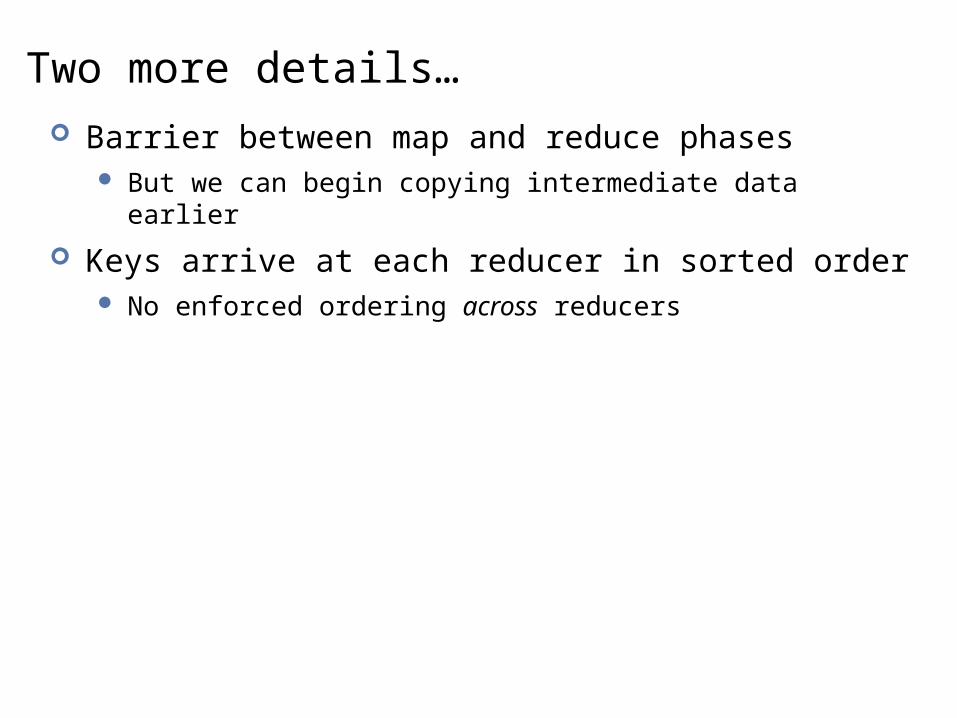
Two more details… Barrier between map and reduce phases
But we can begin copying intermediate data earlier
Keys arrive at each reducer in sorted order No enforced ordering across reducers
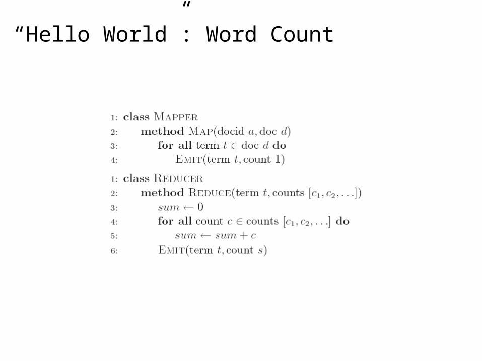
“Hello World”: Word Count
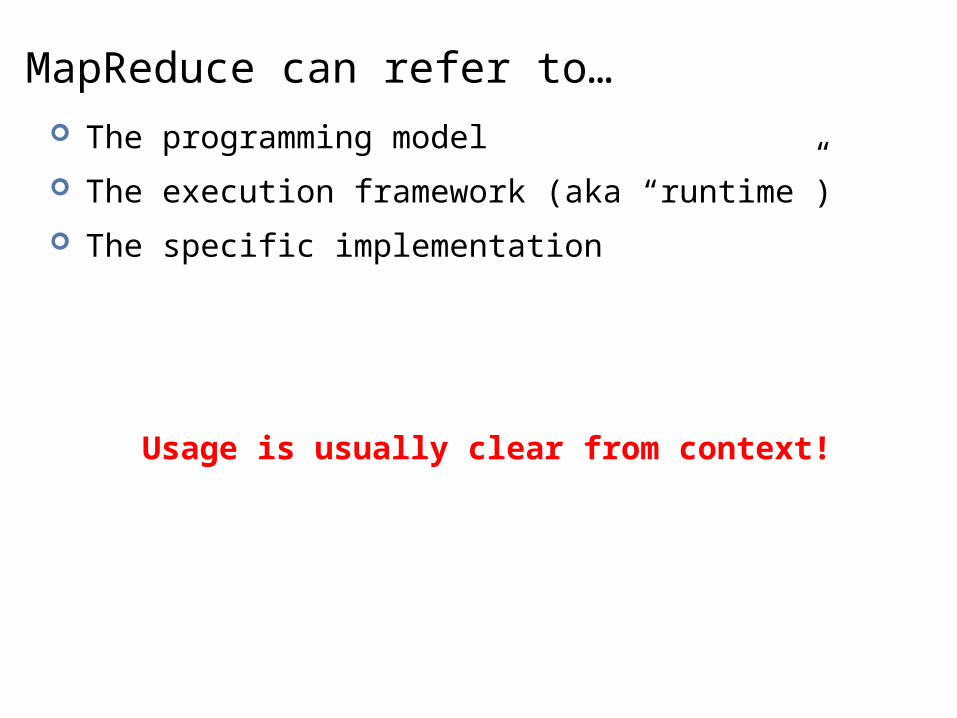
MapReduce can refer to… The programming model
The execution framework (aka “runtime”)
The specific implementation
Usage is usually clear from context!

MapReduce Implementations Google has a proprietary implementation in C++
Bindings in Java, Python
Hadoop is an open-source implementation in Java Original development led by Yahoo Now an Apache open source project Emerging as the de facto big data stack Rapidly expanding software ecosystem
Lots of custom research implementations For GPUs, cell processors, etc. Includes variations of the basic programming model
Most of these slides are focused on Hadoop

split 0
split 1
split 2
split 3
split 4
worker
worker
worker
worker
worker
Master
UserProgram
outputfile 0
outputfile 1
(1) submit
(2) schedule map (2) schedule reduce
(3) read(4) local write
(5) remote read(6) write
Inputfiles
Mapphase
Intermediate files(on local disk)
Reducephase
Outputfiles
Adapted from (Dean and Ghemawat, OSDI 2004)
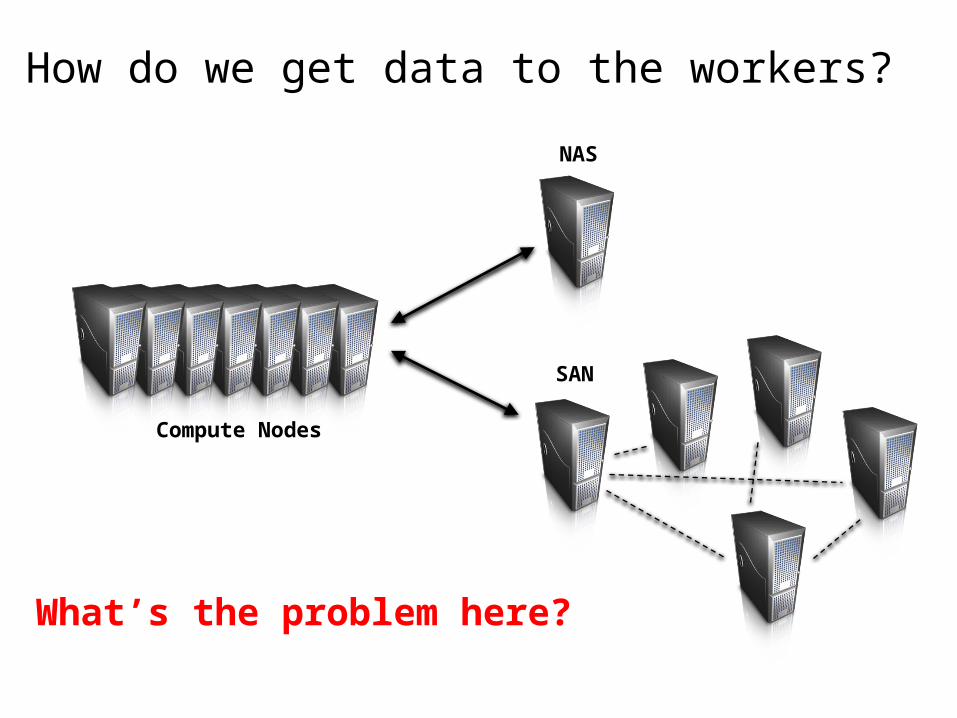
How do we get data to the workers?
Compute Nodes
NAS
SAN
What’s the problem here?

Distributed File System Don’t move data to workers… move workers to the data!
Store data on the local disks of nodes in the cluster Start up the workers on the node that has the data local
A distributed file system is the answer GFS (Google File System) for Google’s MapReduce HDFS (Hadoop Distributed File System) for Hadoop

GFS: Assumptions Commodity hardware over “exotic” hardware
Scale “out”, not “up”
High component failure rates Inexpensive commodity components fail all the time
“Modest” number of huge files Multi-gigabyte files are common, if not encouraged
Files are write-once, mostly appended to Perhaps concurrently
Large streaming reads over random access High sustained throughput over low latency
GFS slides adapted from material by (Ghemawat et al., SOSP 2003)

GFS: Design Decisions Files stored as chunks
Fixed size (64MB)
Reliability through replication Each chunk replicated across 3+ chunkservers
Single master to coordinate access, keep metadata Simple centralized management
No data caching Little benefit due to large datasets, streaming reads
Simplify the API Push some of the issues onto the client (e.g., data layout)
HDFS = GFS clone (same basic ideas)
From GFS to HDFS Terminology differences:
GFS master = Hadoop namenode GFS chunkservers = Hadoop datanodes
Functional differences: File appends in HDFS is relatively new HDFS performance is (likely) slower
For the most part, we’ll use the Hadoop terminology…

Adapted from (Ghemawat et al., SOSP 2003)
(file name, block id)
(block id, block location)
instructions to datanode
datanode state(block id, byte range)
block data
HDFS namenode
HDFS datanode
Linux file system
…
HDFS datanode
Linux file system
…
File namespace/foo/bar
block 3df2
Application
HDFS Client
HDFS Architecture

Namenode Responsibilities Managing the file system namespace:
Holds file/directory structure, metadata, file-to-block mapping, access permissions, etc.
Coordinating file operations: Directs clients to datanodes for reads and writes No data is moved through the namenode
Maintaining overall health: Periodic communication with the datanodes Block re-replication and rebalancing Garbage collection

Putting everything together…
datanode daemon
Linux file system
…
tasktracker
slave node
datanode daemon
Linux file system
…
tasktracker
slave node
datanode daemon
Linux file system
…
tasktracker
slave node
namenode
namenode daemon
job submission node
jobtracker

MapReduce Algorithm Design
Setting the stageIntroduction to MapReduceMapReduce algorithm designText retrievalManaging relational dataGraph algorithmsBeyond MapReduce

MapReduce: Recap Programmers must specify:
map (k, v) → <k’, v’>*reduce (k’, v’) → <k’, v’>* All values with the same key are reduced together
Optionally, also:partition (k’, number of partitions) → partition for k’ Often a simple hash of the key, e.g., hash(k’) mod n Divides up key space for parallel reduce operationscombine (k’, v’) → <k’, v’>* Mini-reducers that run in memory after the map phase Used as an optimization to reduce network traffic
The execution framework handles everything else…

combinecombine combine combine
ba 1 2 c 9 a c5 2 b c7 8
partition partition partition partition
mapmap map map
k1 k2 k3 k4 k5 k6v1 v2 v3 v4 v5 v6
ba 1 2 c c3 6 a c5 2 b c7 8
Shuffle and Sort: aggregate values by keys
reduce reduce reduce
a 1 5 b 2 7 c 2 9 8
r1 s1 r2 s2 r3 s3

“Everything Else” The execution framework handles everything else…
Scheduling: assigns workers to map and reduce tasks “Data distribution”: moves processes to data Synchronization: gathers, sorts, and shuffles intermediate data Errors and faults: detects worker failures and restarts
Limited control over data and execution flow All algorithms must expressed in m, r, c, p
You don’t know: Where mappers and reducers run When a mapper or reducer begins or finishes Which input a particular mapper is processing Which intermediate key a particular reducer is processing

Tools for Synchronization Cleverly-constructed data structures
Bring partial results together
Sort order of intermediate keys Control order in which reducers process keys
Partitioner Control which reducer processes which keys
Preserving state in mappers and reducers Capture dependencies across multiple keys and values

Preserving State
Mapper object
configure
map
close
stateone object per task
Reducer object
configure
reduce
close
state
one call per input key-value pair
one call per intermediate key
API initialization hook
API cleanup hook
Scalable Hadoop Algorithms: Themes Avoid object creation
Inherently costly operation Garbage collection
Avoid buffering Limited heap size Works for small datasets, but won’t scale!

Importance of Local Aggregation Ideal scaling characteristics:
Twice the data, twice the running time Twice the resources, half the running time
Why can’t we achieve this? Synchronization requires communication Communication kills performance
Thus… avoid communication! Reduce intermediate data via local aggregation Combiners can help
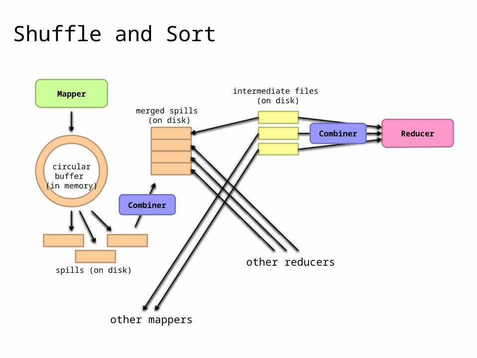
Shuffle and Sort
Mapper
Reducer
other mappers
other reducers
circular buffer (in memory)
spills (on disk)
merged spills (on disk)
intermediate files (on disk)
Combiner
Combiner
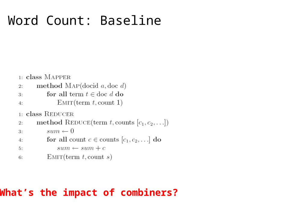
Word Count: Baseline
What’s the impact of combiners?
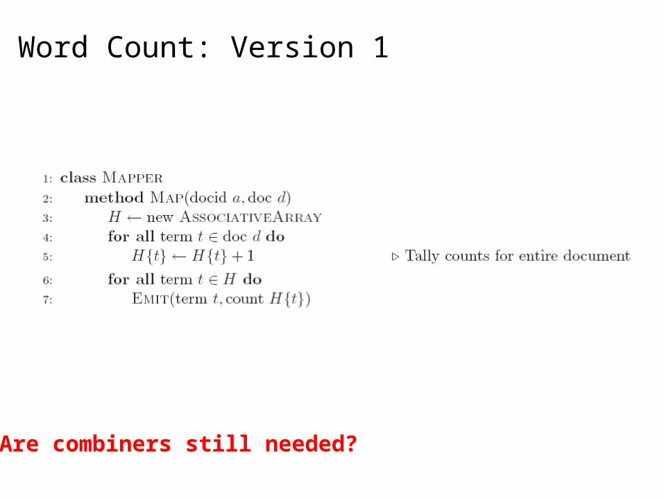
Word Count: Version 1
Are combiners still needed?

Word Count: Version 2
Are combiners still needed?
Key: preserve state across
input key-value pairs!

Design Pattern for Local Aggregation “In-mapper combining”
Fold the functionality of the combiner into the mapper by preserving state across multiple map calls
Advantages Speed Why is this faster than actual combiners?
Disadvantages Explicit memory management required Potential for order-dependent bugs
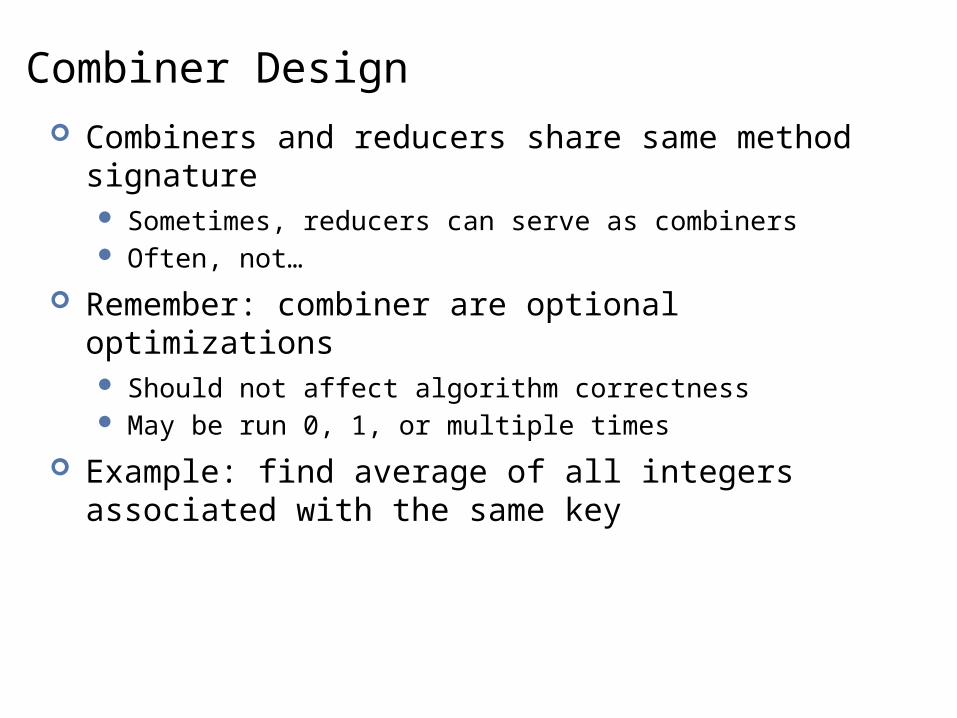
Combiner Design Combiners and reducers share same method signature
Sometimes, reducers can serve as combiners Often, not…
Remember: combiner are optional optimizations Should not affect algorithm correctness May be run 0, 1, or multiple times
Example: find average of all integers associated with the same key
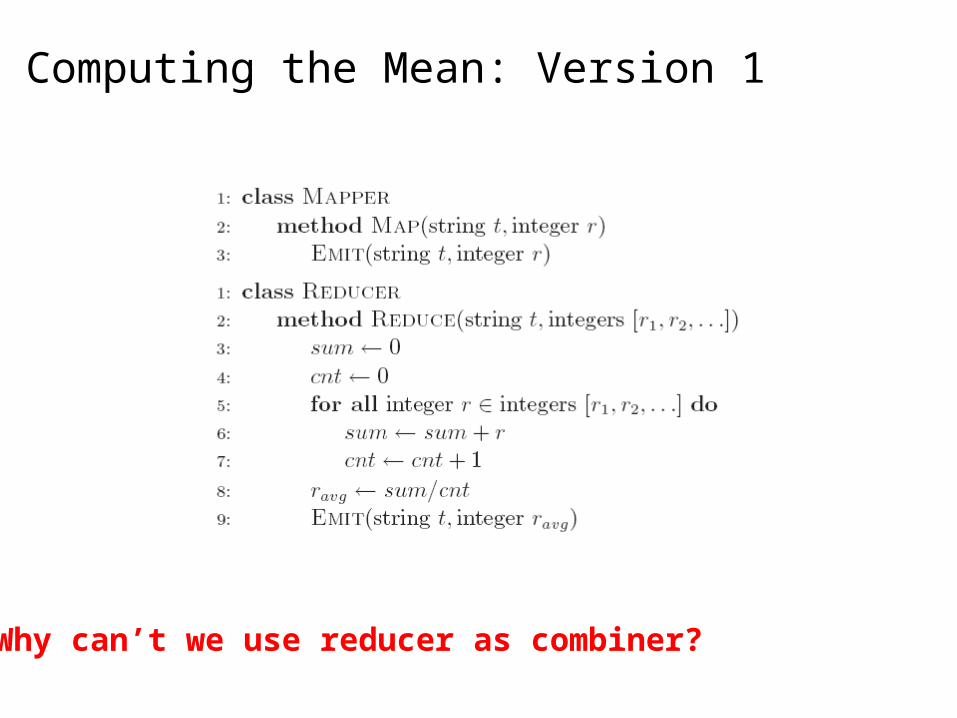
Computing the Mean: Version 1
Why can’t we use reducer as combiner?
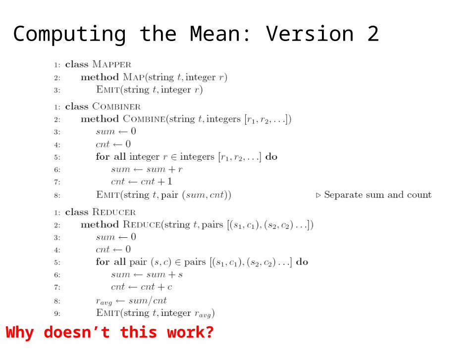
Computing the Mean: Version 2
Why doesn’t this work?

Computing the Mean: Version 3
Fixed?
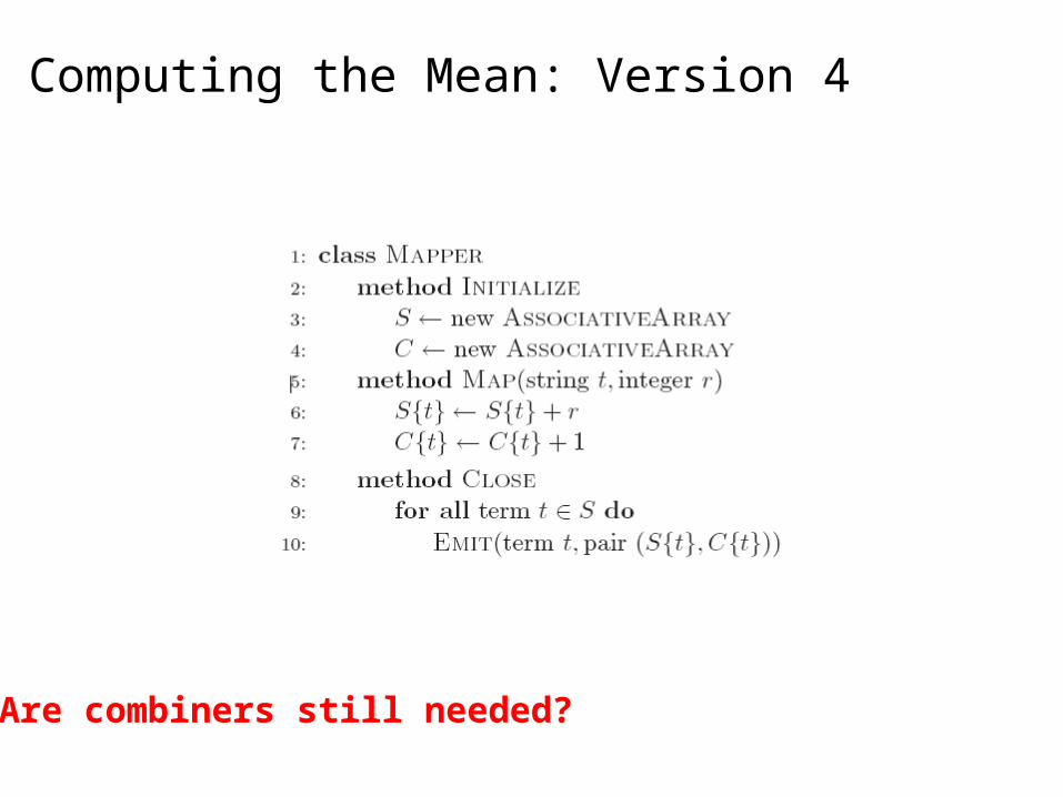
Computing the Mean: Version 4
Are combiners still needed?

“Count and Normalize” Many algorithms reduce to estimating relative frequencies:
In the case of EM, pseudo-counts instead of actual counts
For a large class of algorithms: intuition is the same, just varying complexity in terms of bookkeeping
Let’s start with the intuition…
'
)',(count
),(count
)(count
),(count)|(
B
BA
BA
A
BAABf
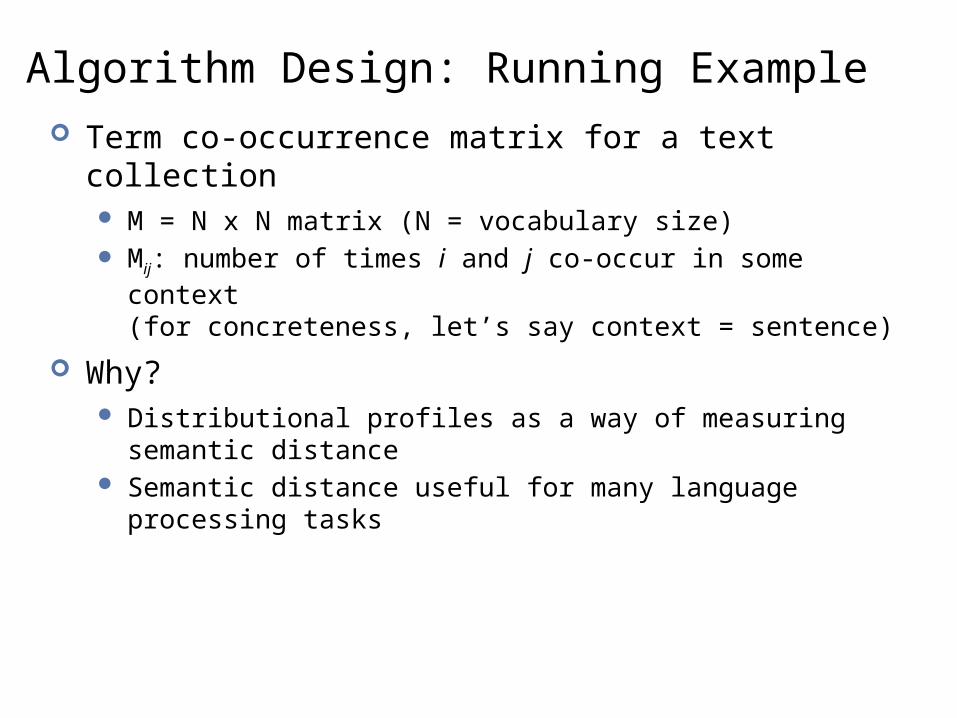
Algorithm Design: Running Example Term co-occurrence matrix for a text collection
M = N x N matrix (N = vocabulary size) Mij: number of times i and j co-occur in some context
(for concreteness, let’s say context = sentence)
Why? Distributional profiles as a way of measuring semantic distance Semantic distance useful for many language processing tasks
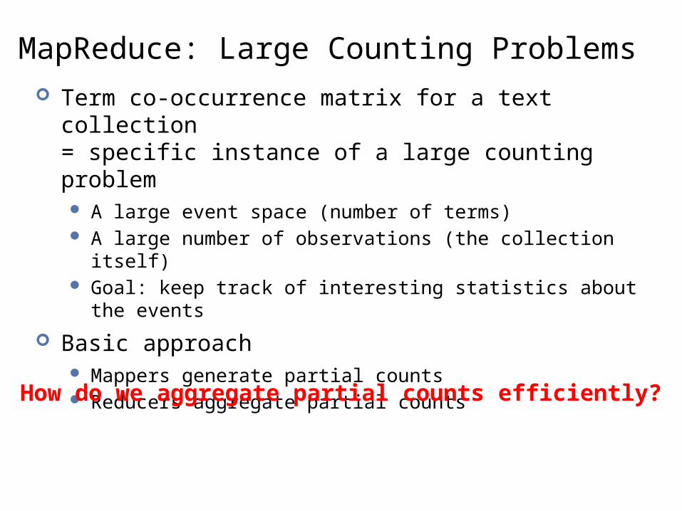
MapReduce: Large Counting Problems Term co-occurrence matrix for a text collection
= specific instance of a large counting problem A large event space (number of terms) A large number of observations (the collection itself) Goal: keep track of interesting statistics about the events
Basic approach Mappers generate partial counts Reducers aggregate partial counts
How do we aggregate partial counts efficiently?
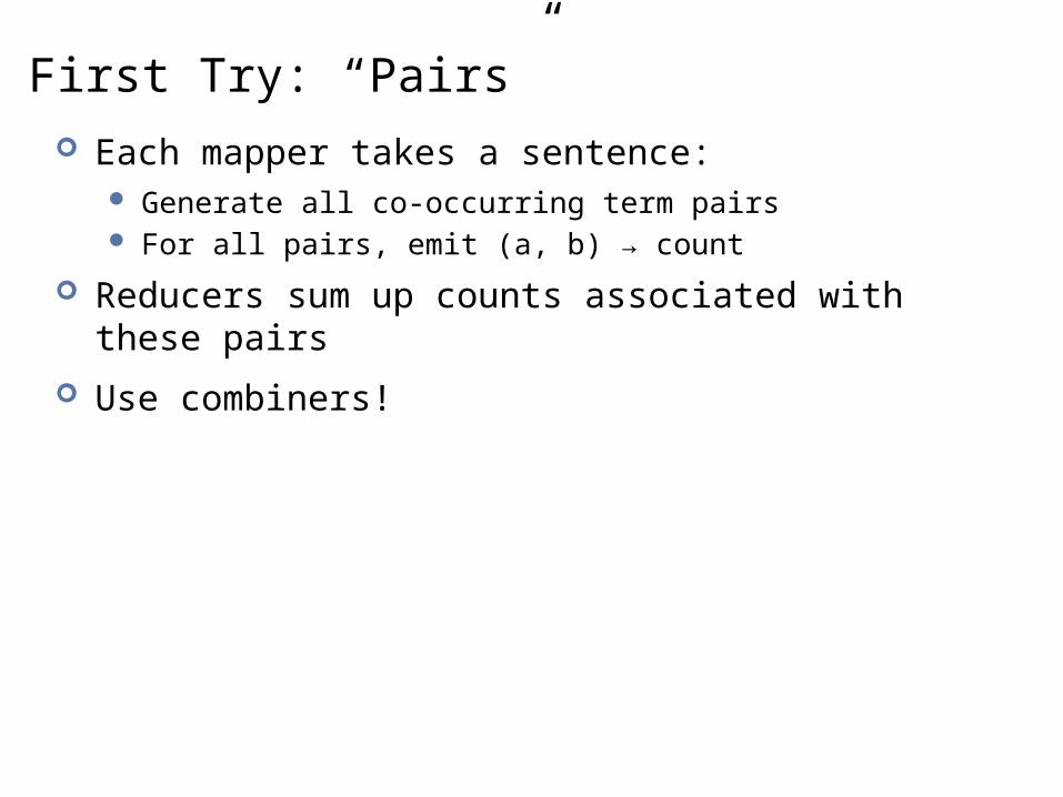
First Try: “Pairs” Each mapper takes a sentence:
Generate all co-occurring term pairs For all pairs, emit (a, b) → count
Reducers sum up counts associated with these pairs
Use combiners!

Pairs: Pseudo-Code
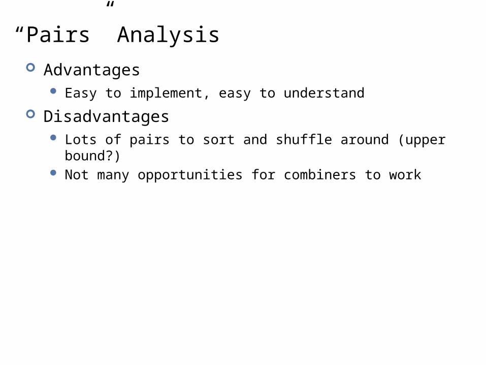
“Pairs” Analysis Advantages
Easy to implement, easy to understand
Disadvantages Lots of pairs to sort and shuffle around (upper bound?) Not many opportunities for combiners to work
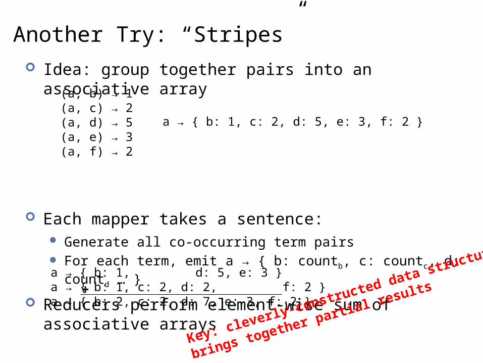
Another Try: “Stripes” Idea: group together pairs into an associative array
Each mapper takes a sentence: Generate all co-occurring term pairs For each term, emit a → { b: countb, c: countc, d: countd … }
Reducers perform element-wise sum of associative arrays
(a, b) → 1 (a, c) → 2 (a, d) → 5 (a, e) → 3 (a, f) → 2
a → { b: 1, c: 2, d: 5, e: 3, f: 2 }
a → { b: 1, d: 5, e: 3 }a → { b: 1, c: 2, d: 2, f: 2 }a → { b: 2, c: 2, d: 7, e: 3, f: 2 }
+
Key: cleverly-constructed data structure
brings together partial results
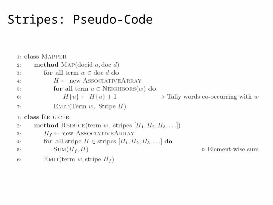
Stripes: Pseudo-Code
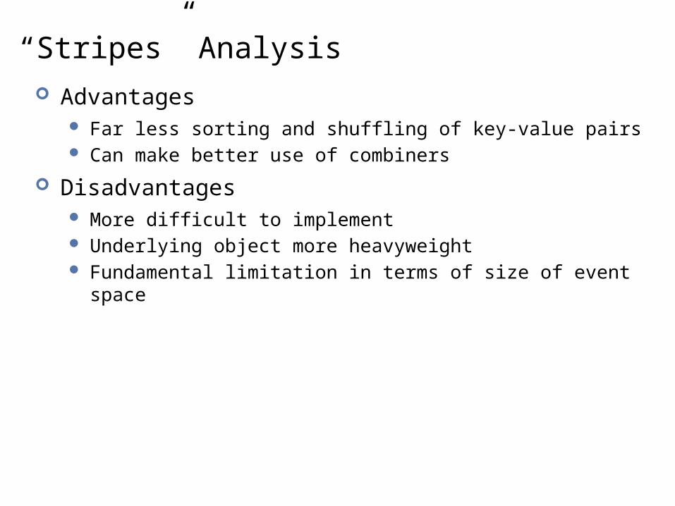
“Stripes” Analysis Advantages
Far less sorting and shuffling of key-value pairs Can make better use of combiners
Disadvantages More difficult to implement Underlying object more heavyweight Fundamental limitation in terms of size of event space
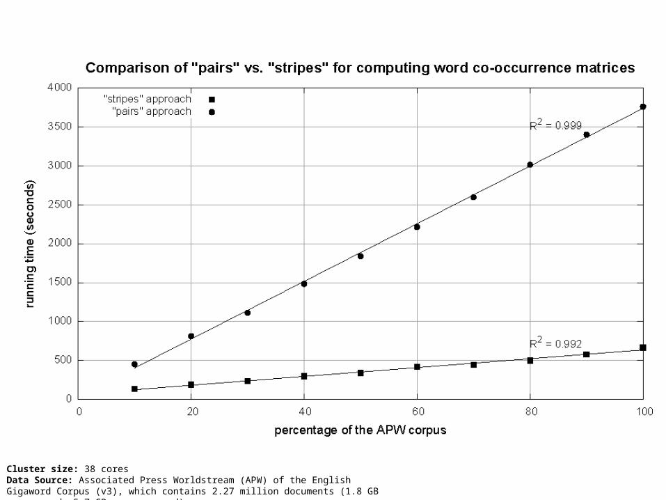
Cluster size: 38 coresData Source: Associated Press Worldstream (APW) of the English Gigaword Corpus (v3), which contains 2.27 million documents (1.8 GB compressed, 5.7 GB uncompressed)

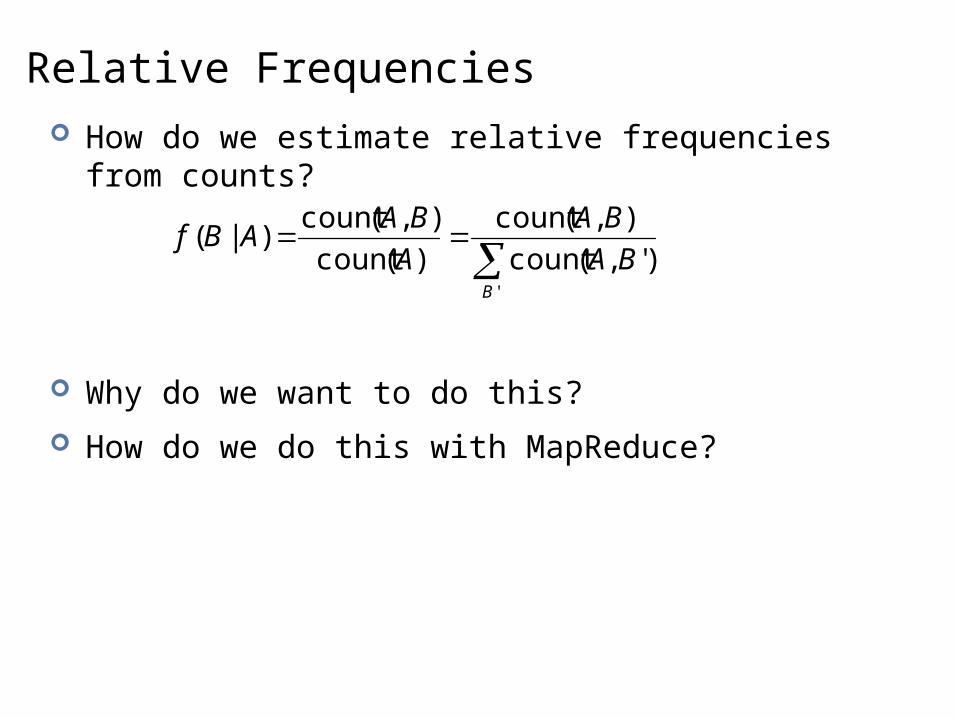
Relative Frequencies How do we estimate relative frequencies from counts?
Why do we want to do this?
How do we do this with MapReduce?
'
)',(count
),(count
)(count
),(count)|(
B
BA
BA
A
BAABf

f(B|A): “Stripes”
Easy! One pass to compute (a, *) Another pass to directly compute f(B|A)
a → {b1:3, b2 :12, b3 :7, b4 :1, … }
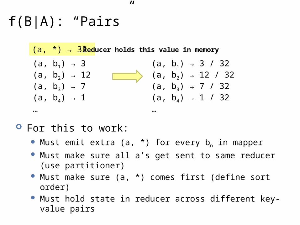
f(B|A): “Pairs”
For this to work: Must emit extra (a, *) for every bn in mapper Must make sure all a’s get sent to same reducer (use partitioner) Must make sure (a, *) comes first (define sort order) Must hold state in reducer across different key-value pairs
(a, b1) → 3 (a, b2) → 12 (a, b3) → 7(a, b4) → 1 …
(a, *) → 32
(a, b1) → 3 / 32 (a, b2) → 12 / 32(a, b3) → 7 / 32(a, b4) → 1 / 32…
Reducer holds this value in memory
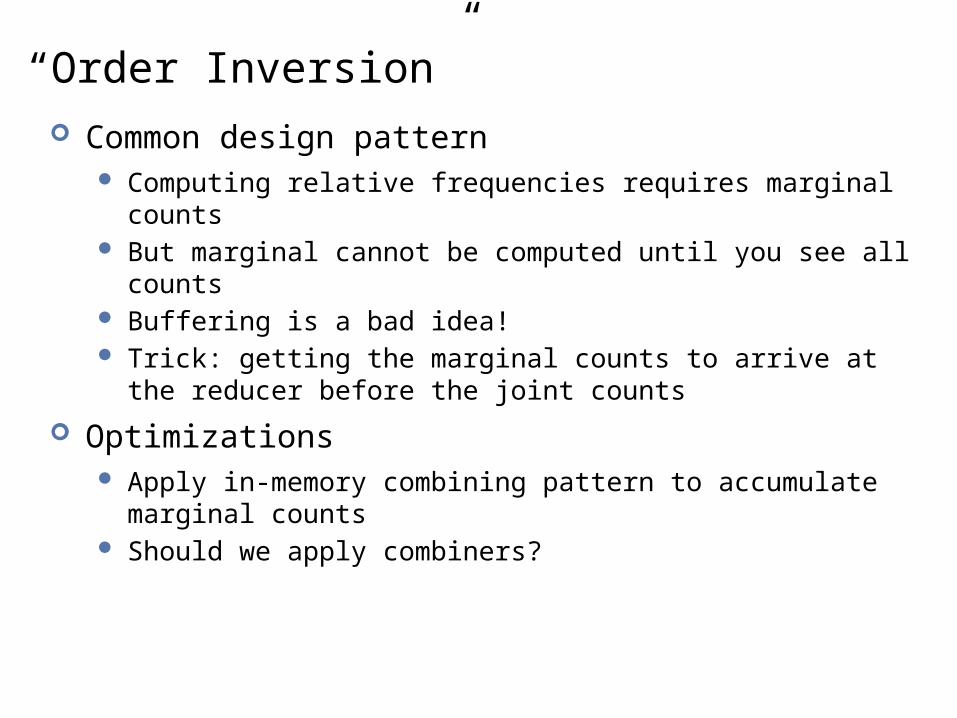
“Order Inversion” Common design pattern
Computing relative frequencies requires marginal counts But marginal cannot be computed until you see all counts Buffering is a bad idea! Trick: getting the marginal counts to arrive at the reducer before
the joint counts
Optimizations Apply in-memory combining pattern to accumulate marginal counts Should we apply combiners?
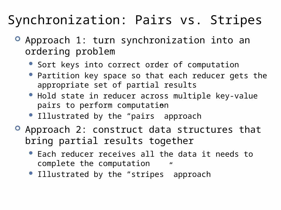
Synchronization: Pairs vs. Stripes Approach 1: turn synchronization into an ordering problem
Sort keys into correct order of computation Partition key space so that each reducer gets the appropriate set
of partial results Hold state in reducer across multiple key-value pairs to perform
computation Illustrated by the “pairs” approach
Approach 2: construct data structures that bring partial results together Each reducer receives all the data it needs to complete the
computation Illustrated by the “stripes” approach

Secondary Sorting MapReduce sorts input to reducers by key
Values may be arbitrarily ordered
What if want to sort value also? E.g., k → (v1, r), (v3, r), (v4, r), (v8, r)…
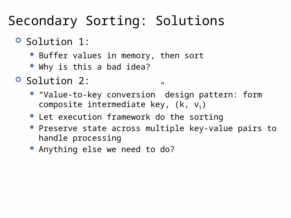
Secondary Sorting: Solutions Solution 1:
Buffer values in memory, then sort Why is this a bad idea?
Solution 2: “Value-to-key conversion” design pattern: form composite
intermediate key, (k, v1) Let execution framework do the sorting Preserve state across multiple key-value pairs to handle
processing Anything else we need to do?

Recap: Tools for Synchronization Cleverly-constructed data structures
Bring data together
Sort order of intermediate keys Control order in which reducers process keys
Partitioner Control which reducer processes which keys
Preserving state in mappers and reducers Capture dependencies across multiple keys and values
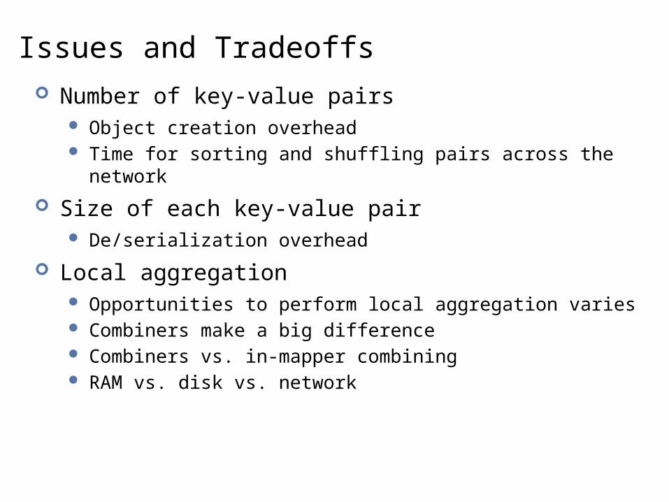
Issues and Tradeoffs Number of key-value pairs
Object creation overhead Time for sorting and shuffling pairs across the network
Size of each key-value pair De/serialization overhead
Local aggregation Opportunities to perform local aggregation varies Combiners make a big difference Combiners vs. in-mapper combining RAM vs. disk vs. network

Text Retrieval
Setting the stageIntroduction to MapReduceMapReduce algorithm designText retrievalManaging relational dataGraph algorithmsBeyond MapReduce

Abstract IR Architecture
DocumentsQuery
Hits
RepresentationFunction
RepresentationFunction
Query Representation Document Representation
ComparisonFunction Index
offlineonline
document acquisition
(e.g., web crawling)
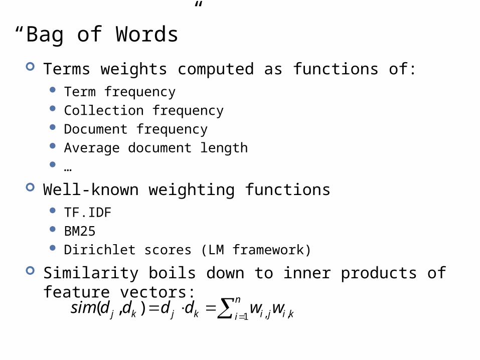
“Bag of Words” Terms weights computed as functions of:
Term frequency Collection frequency Document frequency Average document length …
Well-known weighting functions TF.IDF BM25 Dirichlet scores (LM framework)
Similarity boils down to inner products of feature vectors:
n
i kijikjkj wwddddsim1 ,,),(

2
1
1
2
1
1
1
1
1
1
1
Inverted Index
2
1
2
1
1
1
1 2 3
1
1
1
4
1
1
1
1
1
1
2
1
tfdf
blue
cat
egg
fish
green
ham
hat
one
1
1
1
1
1
1
2
1
blue
cat
egg
fish
green
ham
hat
one
1 1red
1 1two
1red
1two
one fish, two fishDoc 1
red fish, blue fishDoc 2
cat in the hatDoc 3
green eggs and hamDoc 4
3
4
1
4
4
3
2
1
2
2
1

[2,4]
[3]
[2,4]
[2]
[1]
[1]
[3]
[2]
[1]
[1]
[3]
2
1
1
2
1
1
1
1
1
1
1
Inverted Index: Positional Information
2
1
2
1
1
1
1 2 3
1
1
1
4
1
1
1
1
1
1
2
1
tfdf
blue
cat
egg
fish
green
ham
hat
one
1
1
1
1
1
1
2
1
blue
cat
egg
fish
green
ham
hat
one
1 1red
1 1two
1red
1two
one fish, two fishDoc 1
red fish, blue fishDoc 2
cat in the hatDoc 3
green eggs and hamDoc 4
3
4
1
4
4
3
2
1
2
2
1

Retrieval in a Nutshell Look up postings lists corresponding to query terms
Traverse postings for each query term
Store partial query-document scores in accumulators
Select top k results to return
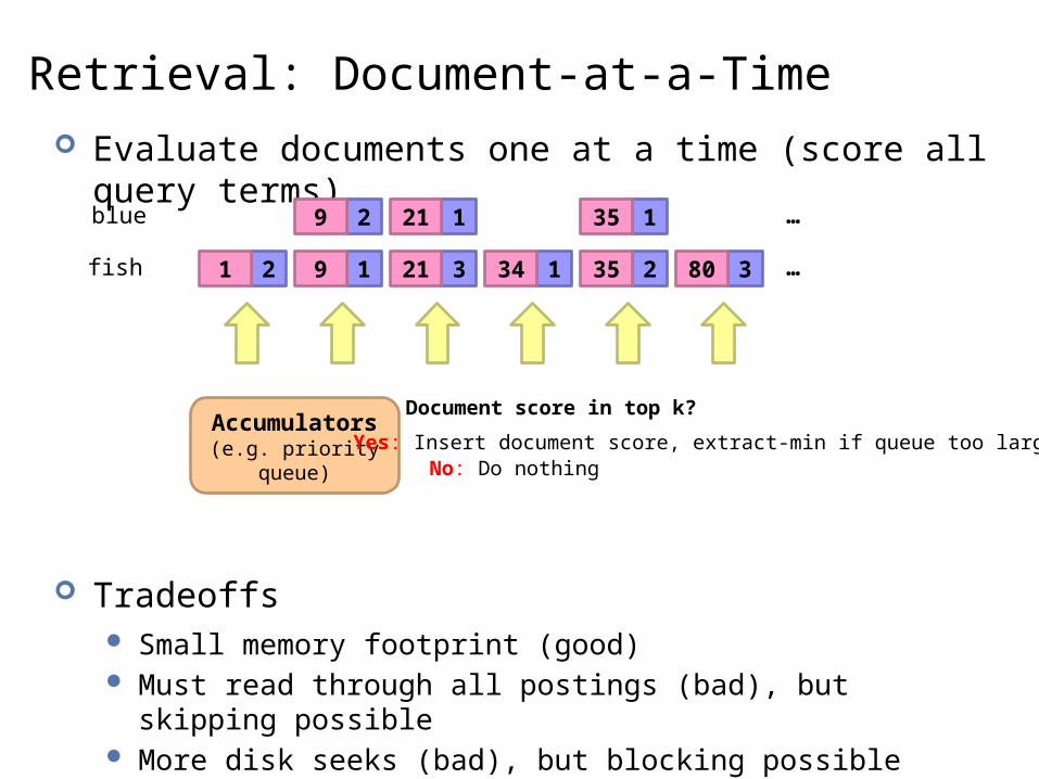
Retrieval: Document-at-a-Time Evaluate documents one at a time (score all query terms)
Tradeoffs Small memory footprint (good) Must read through all postings (bad), but skipping possible More disk seeks (bad), but blocking possible
fish 2 1 3 1 2 31 9 21 34 35 80 …
blue 2 1 19 21 35 …
Accumulators(e.g. priority queue)
Document score in top k?
Yes: Insert document score, extract-min if queue too largeNo: Do nothing
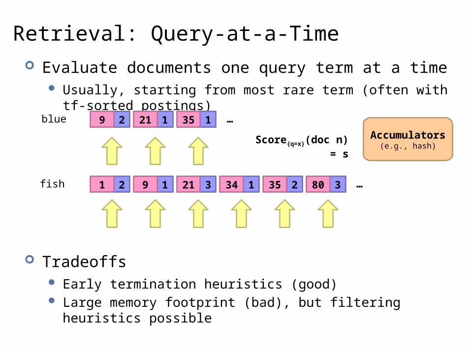
Retrieval: Query-at-a-Time Evaluate documents one query term at a time
Usually, starting from most rare term (often with tf-sorted postings)
Tradeoffs Early termination heuristics (good) Large memory footprint (bad), but filtering heuristics possible
fish 2 1 3 1 2 31 9 21 34 35 80 …
blue 2 1 19 21 35 …
Accumulators(e.g., hash)
Score{q=x}(doc n) = s
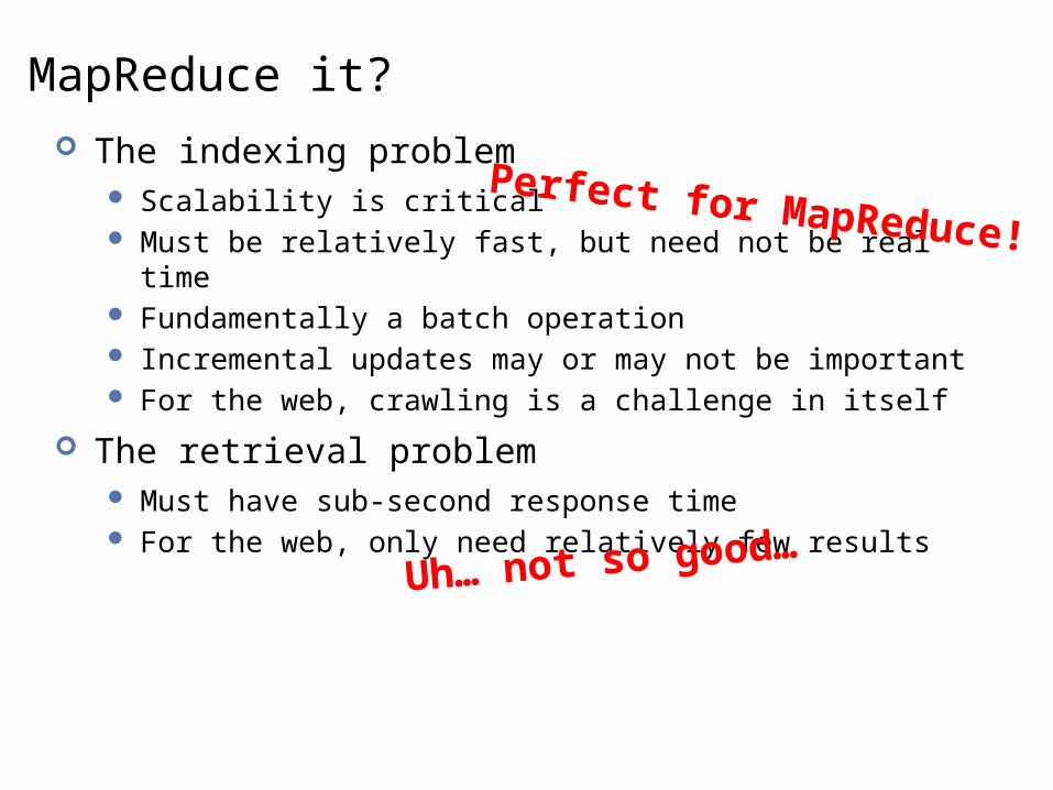
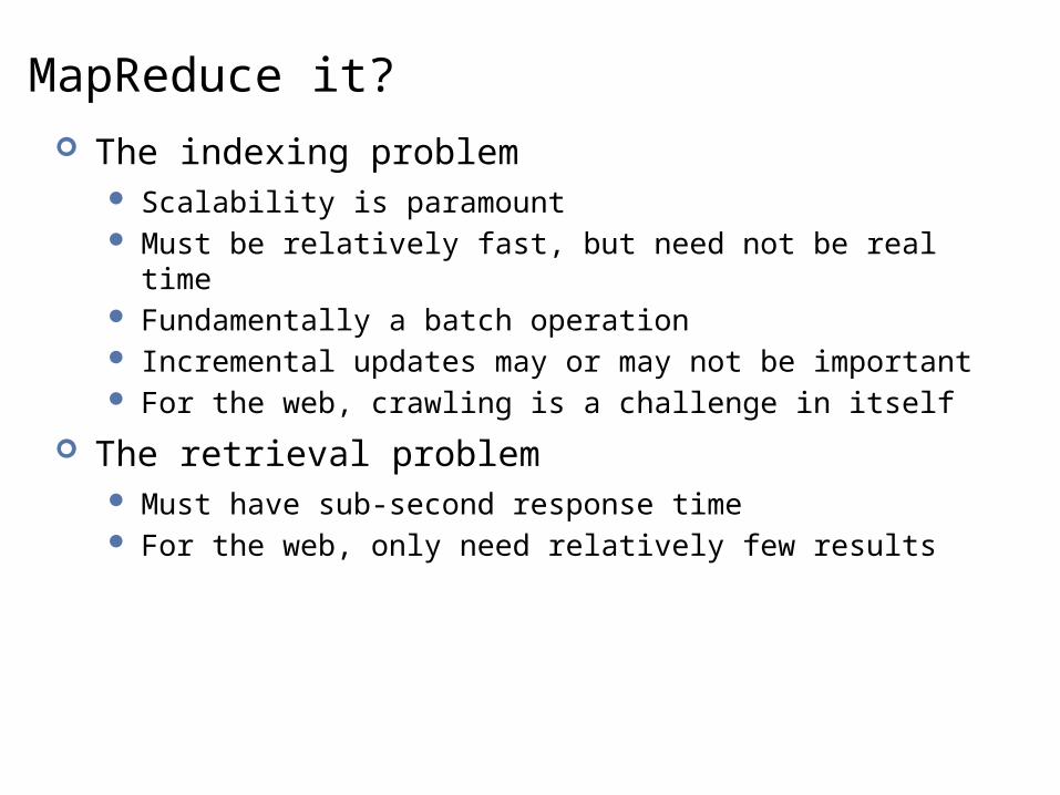
MapReduce it? The indexing problem
Scalability is critical Must be relatively fast, but need not be real time Fundamentally a batch operation Incremental updates may or may not be important For the web, crawling is a challenge in itself
The retrieval problem Must have sub-second response time For the web, only need relatively few results
Perfect for MapReduce!
Uh… not so good…
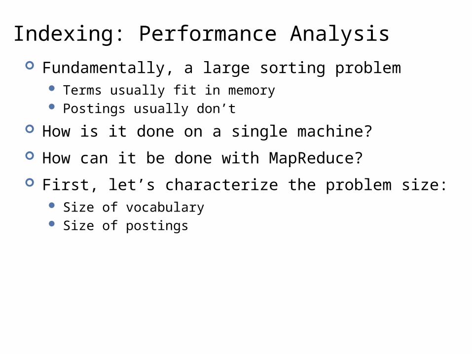
Indexing: Performance Analysis Fundamentally, a large sorting problem
Terms usually fit in memory Postings usually don’t
How is it done on a single machine?
How can it be done with MapReduce?
First, let’s characterize the problem size: Size of vocabulary Size of postings

Vocabulary Size: Heaps’ Law
Heaps’ Law: linear in log-log space
Vocabulary size grows unbounded!
bkTM M is vocabulary sizeT is collection size (number of documents)k and b are constants
Typically, k is between 30 and 100, b is between 0.4 and 0.6
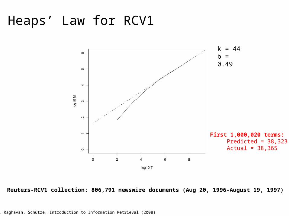
Heaps’ Law for RCV1
Reuters-RCV1 collection: 806,791 newswire documents (Aug 20, 1996-August 19, 1997)
k = 44b = 0.49
First 1,000,020 terms: Predicted = 38,323 Actual = 38,365
Manning, Raghavan, Schütze, Introduction to Information Retrieval (2008)

Postings Size: Zipf’s Law
Zipf’s Law: (also) linear in log-log space Specific case of Power Law distributions
In other words: A few elements occur very frequently Many elements occur very infrequently
i
ci cf cf is the collection frequency of i-th common term
c is a constant
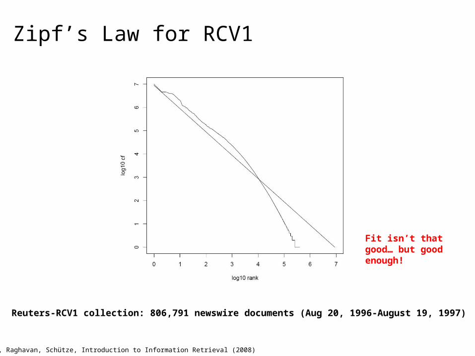
Zipf’s Law for RCV1
Reuters-RCV1 collection: 806,791 newswire documents (Aug 20, 1996-August 19, 1997)
Fit isn’t that good… but good enough!
Manning, Raghavan, Schütze, Introduction to Information Retrieval (2008)

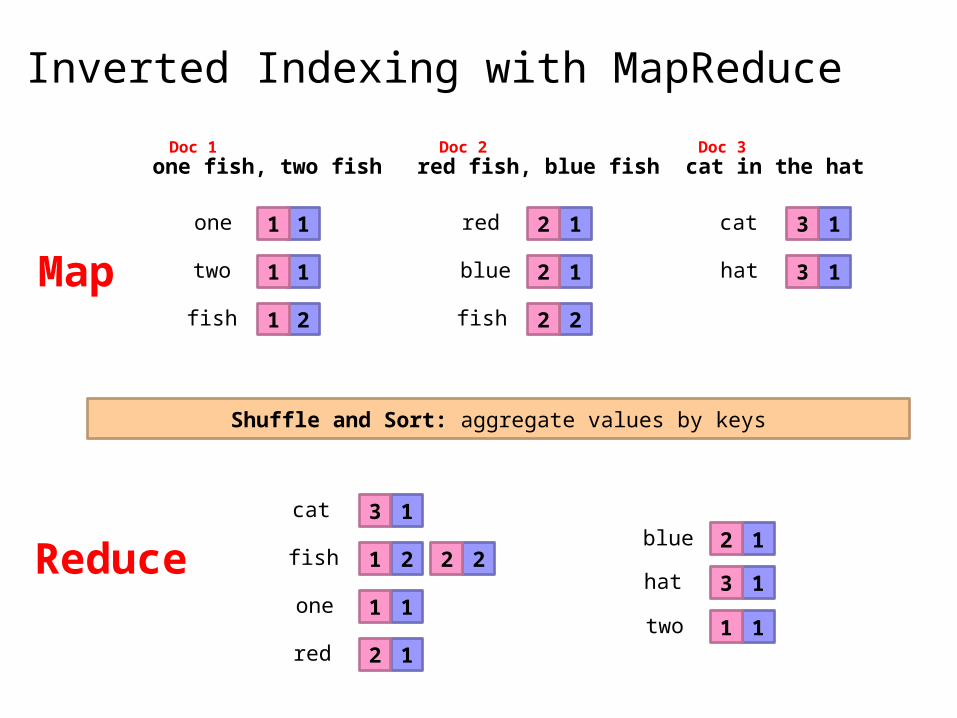
MapReduce: Index Construction Map over all documents
Emit term as key, (docno, tf) as value Emit other information as necessary (e.g., term position)
Sort/shuffle: group postings by term
Reduce Gather and sort the postings (e.g., by docno or tf) Write postings to disk
MapReduce does all the heavy lifting!
1
1
2
1
1
2 2
11
1
11
1
1
1
2
Inverted Indexing with MapReduce
1one
1two
1fish
one fish, two fishDoc 1
2red
2blue
2fish
red fish, blue fishDoc 2
3cat
3hat
cat in the hatDoc 3
1fish 2
1one1two
2red
3cat
2blue
3hat
Shuffle and Sort: aggregate values by keys
Map
Reduce
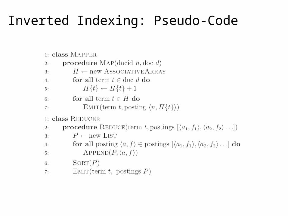
Inverted Indexing: Pseudo-Code
[2,4]
[1]
[3]
[1]
[2]
[1]
[1]
[3]
[2]
[3]
[2,4]
[1]
[2,4]
[2,4]
[1]
[3]
1
1
2
1
1
2
1
1
2 2
11
1
11
1
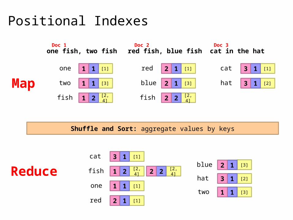
Positional Indexes
1one
1two
1fish
2red
2blue
2fish
3cat
3hat
1fish 2
1one1two
2red
3cat2blue
3hat
Shuffle and Sort: aggregate values by keys
Map
Reduce
one fish, two fishDoc 1
red fish, blue fishDoc 2
cat in the hatDoc 3
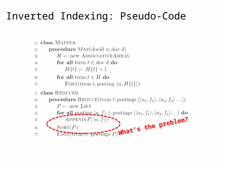
Inverted Indexing: Pseudo-Code
What’s the problem?
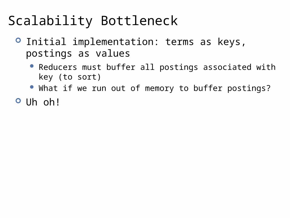
Scalability Bottleneck Initial implementation: terms as keys, postings as values
Reducers must buffer all postings associated with key (to sort) What if we run out of memory to buffer postings?
Uh oh!

[2,4]
[9]
[1,8,22]
[23]
[8,41]
[2,9,76]
[2,4]
[9]
[1,8,22]
[23]
[8,41]
[2,9,76]
2
1
3
1
2
3
Another Try…
1fish
9
21
(values)(key)
34
35
80
1fish
9
21
(values)(keys)
34
35
80
fish
fish
fish
fish
fish
How is this different?• Let the framework do the sorting• Term frequency implicitly stored• Directly write compressed postings
Where have we seen this before?

2 1 3 1 2 3
2 1 3 1 2 3
Postings Encoding
1fish 9 21 34 35 80 …
1fish 8 12 13 1 45 …
Conceptually:
In Practice:
• Don’t encode docnos, encode gaps (or d-gaps) • But it’s not obvious that this save space…
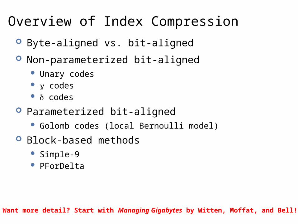
Overview of Index Compression Byte-aligned vs. bit-aligned
Non-parameterized bit-aligned Unary codes codes codes
Parameterized bit-aligned Golomb codes (local Bernoulli model)
Block-based methods Simple-9 PForDelta
Want more detail? Start with Managing Gigabytes by Witten, Moffat, and Bell!

Index Compression: Performance
Witten, Moffat, Bell, Managing Gigabytes (1999)
Unary 262 1918
Binary 15 20
6.51 6.63
6.23 6.38
Golomb 6.09 5.84
Bible TREC
Bible: King James version of the Bible; 31,101 verses (4.3 MB)TREC: TREC disks 1+2; 741,856 docs (2070 MB)
One common approach
Comparison of Index Size (bits per pointer)
Issue: For Golomb compression, optimal b ~ 0.69 (N/df)Which means different b for every term!

Chicken and Egg?
1fish
9
[2,4]
[9]
21 [1,8,22]
(value)(key)
34 [23]
35 [8,41]
80 [2,9,76]
fish
fish
fish
fish
fish
Write directly to disk
But wait! How do we set the Golomb parameter b?
We need the df to set b…
But we don’t know the df until we’ve seen all postings!
…
Optimal b ~ 0.69 (N/df)
Sound familiar?
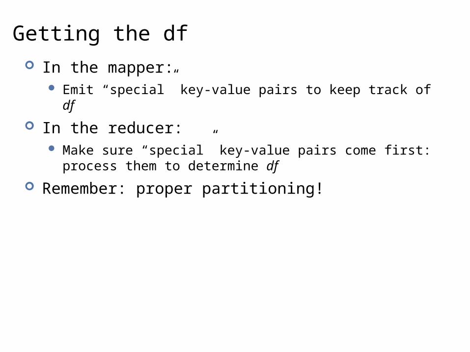
Getting the df In the mapper:
Emit “special” key-value pairs to keep track of df
In the reducer: Make sure “special” key-value pairs come first: process them to
determine df
Remember: proper partitioning!

Getting the df: Modified Mapper
one fish, two fishDoc 1
1fish [2,4]
(value)(key)
1one [1]
1two [3]
fish [1]
one [1]
two [1]
Input document…
Emit normal key-value pairs…
Emit “special” key-value pairs to keep track of df…
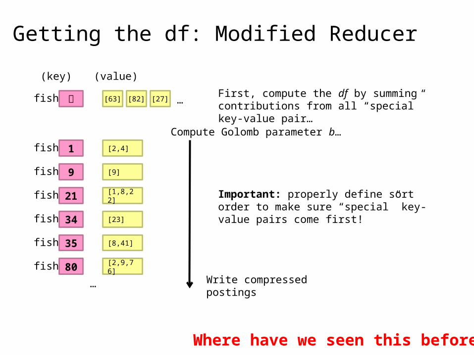
Getting the df: Modified Reducer
1fish
9
[2,4]
[9]
21 [1,8,22]
(value)(key)
34 [23]
35 [8,41]
80 [2,9,76]
fish
fish
fish
fish
fishWrite compressed postings
fish [63] [82] [27] …
…
First, compute the df by summing contributions from all “special” key-value pair…
Compute Golomb parameter b…
Important: properly define sort order to make sure “special” key-value pairs come first!
Where have we seen this before?
MapReduce it? The indexing problem
Scalability is paramount Must be relatively fast, but need not be real time Fundamentally a batch operation Incremental updates may or may not be important For the web, crawling is a challenge in itself
The retrieval problem Must have sub-second response time For the web, only need relatively few results

Retrieval with MapReduce? MapReduce is fundamentally batch-oriented
Optimized for throughput, not latency Startup of mappers and reducers is expensive
MapReduce is not suitable for real-time queries! Use separate infrastructure for retrieval…

Important Ideas Partitioning (for scalability)
Replication (for redundancy)
Caching (for speed)
Routing (for load balancing)
The rest is just details!

Term vs. Document Partitioning
…
T
D
T1
T2
T3
D
T…
D1 D2 D3
Term Partitioning
DocumentPartitioning

partitions
…
…
…
… … … … …
rep
licas
brokers
Typical Search Architecture

Managing Relational Data
Setting the stageIntroduction to MapReduceMapReduce algorithm designText retrievalManaging relational dataGraph algorithmsBeyond MapReduce
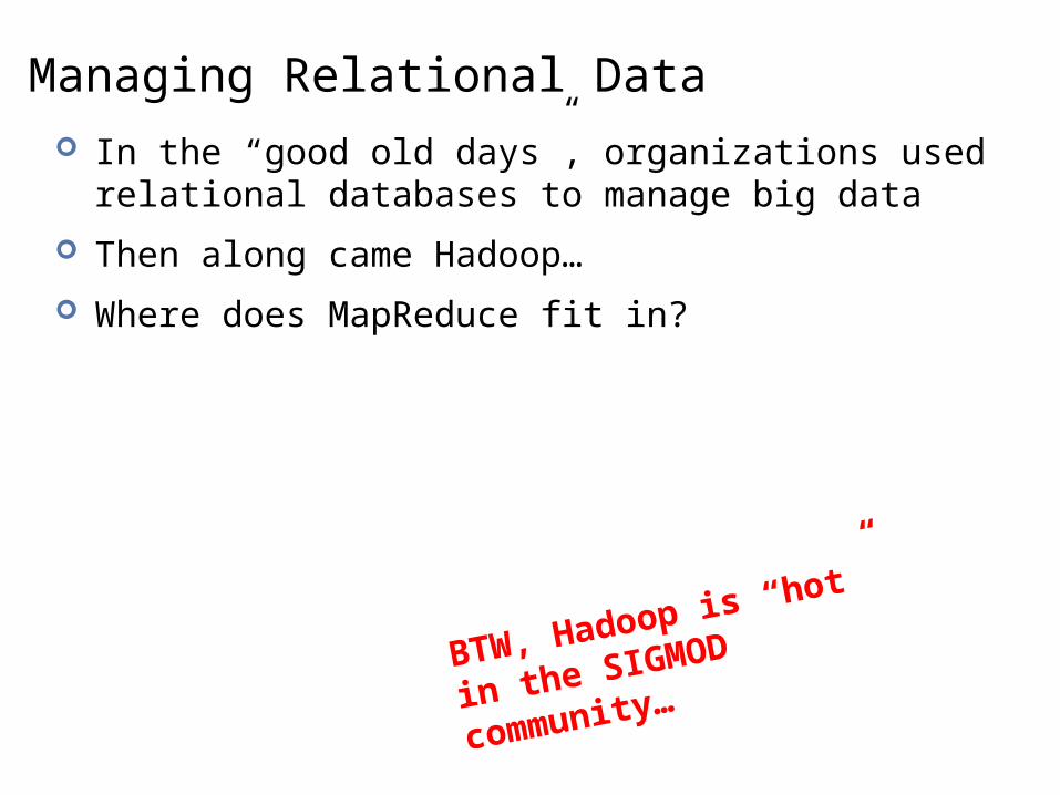
Managing Relational Data In the “good old days”, organizations used relational
databases to manage big data
Then along came Hadoop…
Where does MapReduce fit in?
BTW, Hadoop is “hot” in
the SIGMOD community…
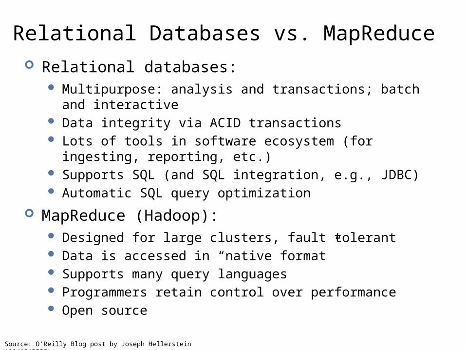
Relational Databases vs. MapReduce Relational databases:
Multipurpose: analysis and transactions; batch and interactive Data integrity via ACID transactions Lots of tools in software ecosystem (for ingesting, reporting, etc.) Supports SQL (and SQL integration, e.g., JDBC) Automatic SQL query optimization
MapReduce (Hadoop): Designed for large clusters, fault tolerant Data is accessed in “native format” Supports many query languages Programmers retain control over performance Open source
Source: O’Reilly Blog post by Joseph Hellerstein (11/19/2008)

Database Workloads OLTP (online transaction processing)
Typical applications: e-commerce, banking, airline reservations User facing: real-time, low latency, highly-concurrent Tasks: relatively small set of “standard” transactional queries Data access pattern: random reads, updates, writes (involving
relatively small amounts of data)
OLAP (online analytical processing) Typical applications: business intelligence, data mining Back-end processing: batch workloads, less concurrency Tasks: complex analytical queries, often ad hoc Data access pattern: table scans, large amounts of data involved
per query

One Database or Two? Downsides of co-existing OLTP and OLAP workloads
Poor memory management Conflicting data access patterns Variable latency
Solution: separate databases User-facing OLTP database for high-volume transactions Data warehouse for OLAP workloads How do we connect the two?

OLTP/OLAP Architecture
OLTP OLAP
ETL(Extract, Transform, and Load)
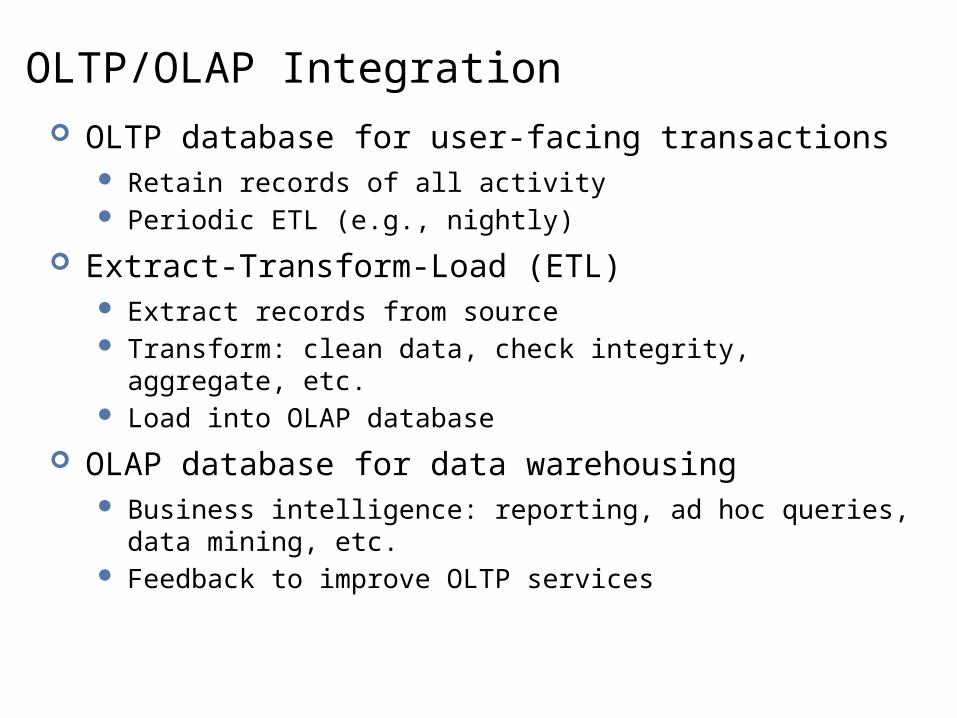
OLTP/OLAP Integration OLTP database for user-facing transactions
Retain records of all activity Periodic ETL (e.g., nightly)
Extract-Transform-Load (ETL) Extract records from source Transform: clean data, check integrity, aggregate, etc. Load into OLAP database
OLAP database for data warehousing Business intelligence: reporting, ad hoc queries, data mining, etc. Feedback to improve OLTP services

Business Intelligence Premise: more data leads to better business decisions
Periodic reporting as well as ad hoc queries Analysts, not programmers (importance of tools and dashboards)
Examples: Slicing-and-dicing activity by different dimensions to better
understand the marketplace Analyzing log data to improve OLTP experience Analyzing log data to better optimize ad placement Analyzing purchasing trends for better supply-chain management Mining for correlations between otherwise unrelated activities

OLTP/OLAP Architecture: Hadoop?
OLTP OLAP
ETL(Extract, Transform, and Load)
Hadoop here?
What about here?
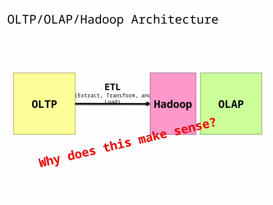
OLTP/OLAP/Hadoop Architecture
OLTP OLAP
ETL(Extract, Transform, and Load)
Hadoop
Why does this make sense?

ETL Bottleneck Reporting is often a nightly task:
ETL is often slow: why? What happens if processing 24 hours of data takes longer than 24
hours?
Hadoop is perfect: Most likely, you already have some data warehousing solution Ingest is limited by speed of HDFS Scales out with more nodes Massively parallel Ability to use any processing tool Much cheaper than parallel databases ETL is a batch process anyway!

Working Scenario Two tables:
User demographics (gender, age, income, etc.) User page visits (URL, time spent, etc.)
Analyses we might want to perform: Statistics on demographic characteristics Statistics on page visits Statistics on page visits by URL Statistics on page visits by demographic characteristic …
How to perform common relational operations in MapReduce… Except, don’t! (later)
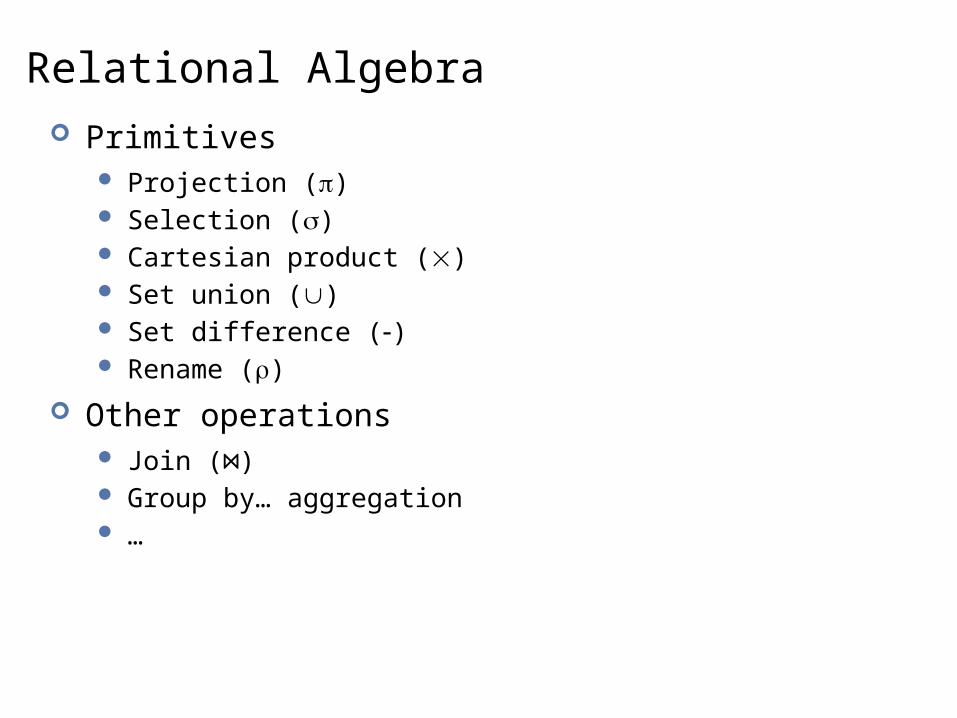
Relational Algebra Primitives
Projection () Selection () Cartesian product () Set union () Set difference () Rename ()
Other operations Join ( )⋈ Group by… aggregation …

Projection
R1
R2
R3
R4
R5
R1
R2
R3
R4
R5
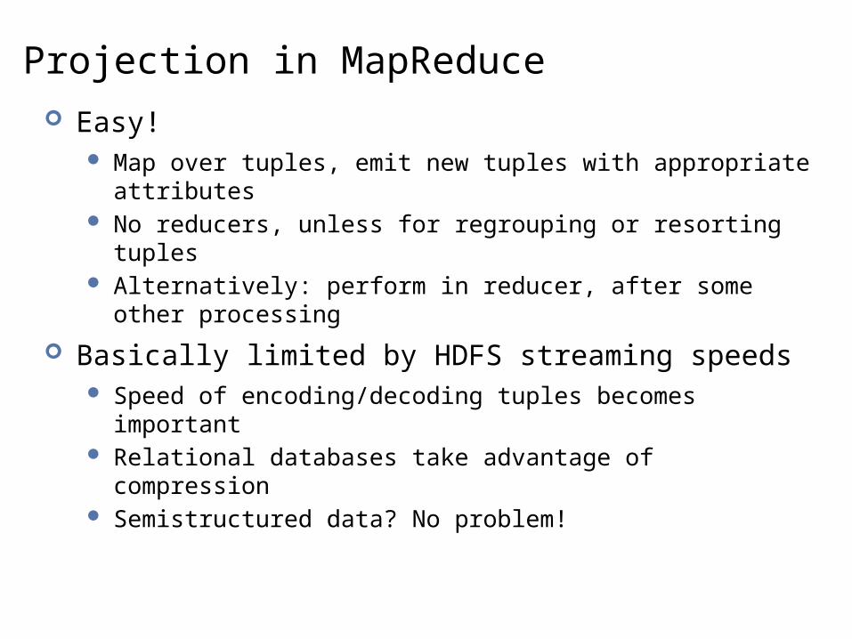
Projection in MapReduce Easy!
Map over tuples, emit new tuples with appropriate attributes No reducers, unless for regrouping or resorting tuples Alternatively: perform in reducer, after some other processing
Basically limited by HDFS streaming speeds Speed of encoding/decoding tuples becomes important Relational databases take advantage of compression Semistructured data? No problem!

Selection
R1
R2
R3
R4
R5
R1
R3

Selection in MapReduce Easy!
Map over tuples, emit only tuples that meet criteria No reducers, unless for regrouping or resorting tuples Alternatively: perform in reducer, after some other processing
Basically limited by HDFS streaming speeds Speed of encoding/decoding tuples becomes important Relational databases take advantage of compression Semistructured data? No problem!
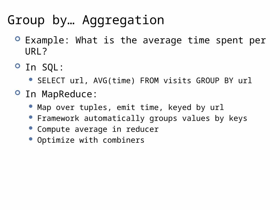
Group by… Aggregation Example: What is the average time spent per URL?
In SQL: SELECT url, AVG(time) FROM visits GROUP BY url
In MapReduce: Map over tuples, emit time, keyed by url Framework automatically groups values by keys Compute average in reducer Optimize with combiners
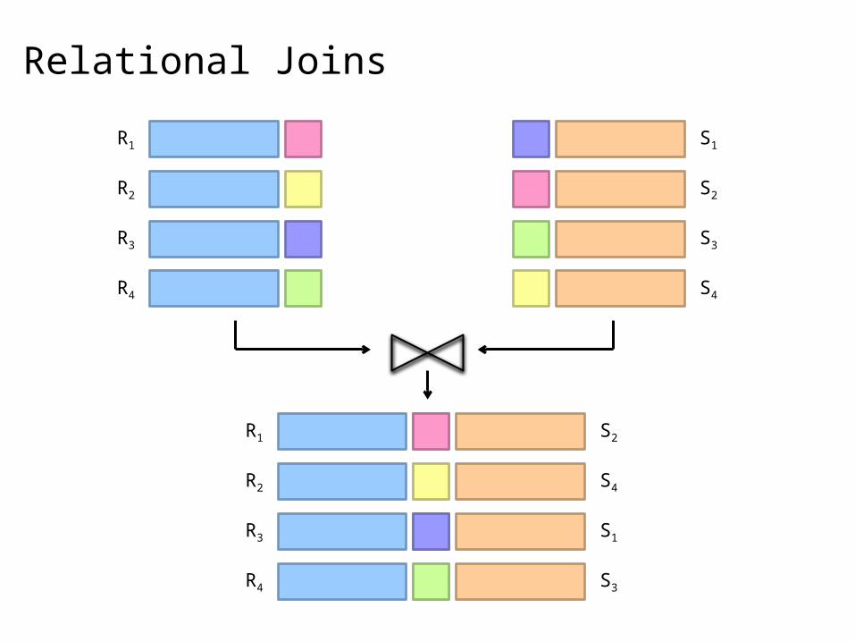
Relational Joins
R1
R2
R3
R4
S1
S2
S3
S4
R1 S2
R2 S4
R3 S1
R4 S3
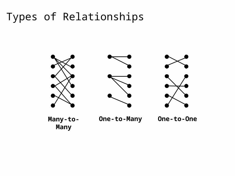
Types of Relationships
One-to-OneOne-to-ManyMany-to-Many

Join Algorithms in MapReduce Reduce-side join
Map-side join
In-memory join Striped variant Memcached variant

Reduce-side Join Basic idea: group by join key
Map over both sets of tuples Emit tuple as value with join key as the intermediate key Execution framework brings together tuples sharing the same key Perform actual join in reducer Similar to a “sort-merge join” in database terminology
Two variants 1-to-1 joins 1-to-many and many-to-many joins
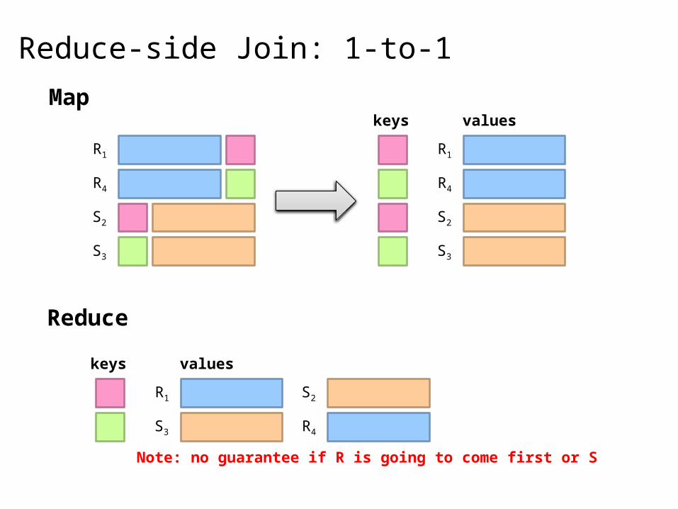
Reduce-side Join: 1-to-1
R1
R4
S2
S3
R1
R4
S2
S3
keys valuesMap
R1
R4
S2
S3
keys values
Reduce
Note: no guarantee if R is going to come first or S
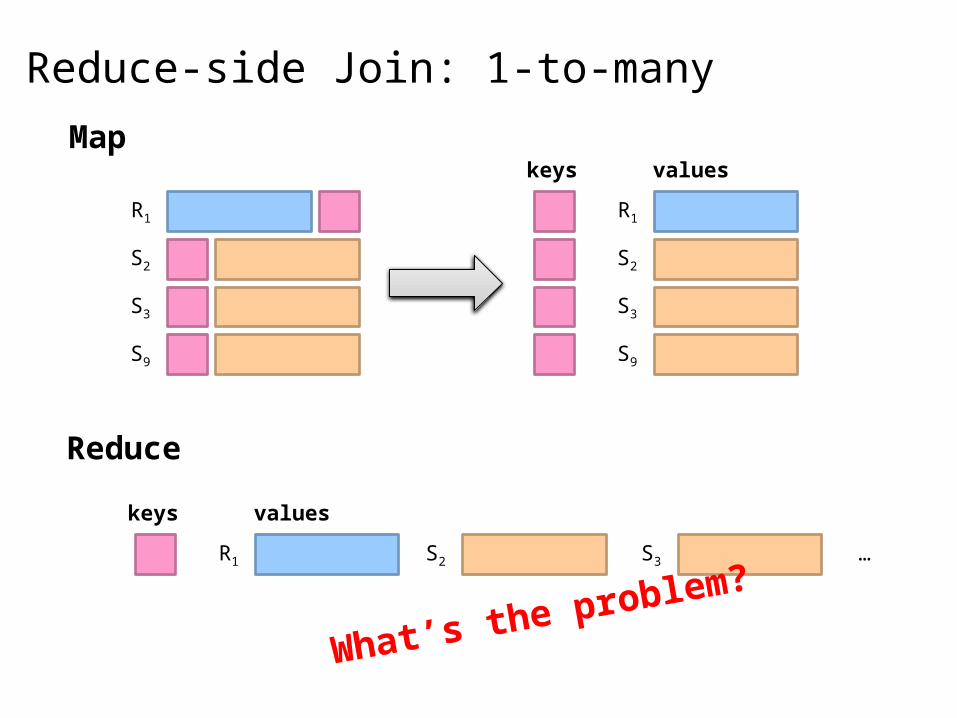
Reduce-side Join: 1-to-many
R1
S2
S3
R1
S2
S3
S9
keys valuesMap
R1 S2
keys values
Reduce
S9
S3 …
What’s the problem?
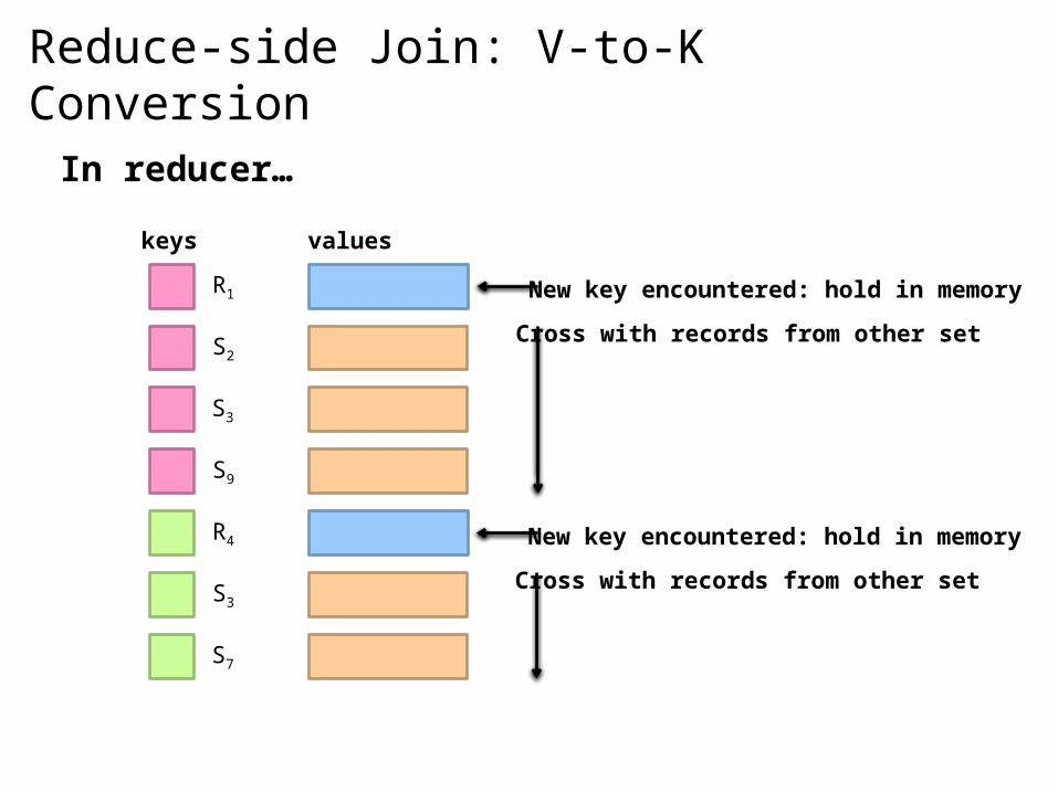
Reduce-side Join: V-to-K Conversion
R1
keys values
In reducer…
S2
S3
S9
R4
S3
S7
New key encountered: hold in memory
Cross with records from other set
New key encountered: hold in memory
Cross with records from other set
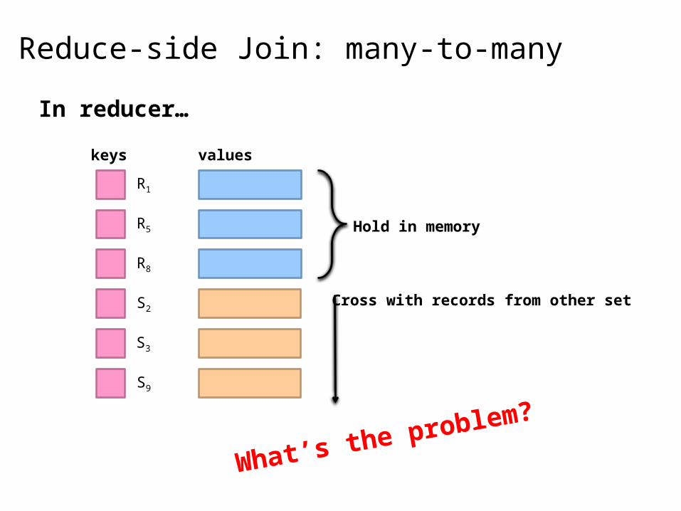
Reduce-side Join: many-to-many
R1
keys values
In reducer…
S2
S3
S9
Hold in memory
Cross with records from other set
R5
R8
What’s the problem?
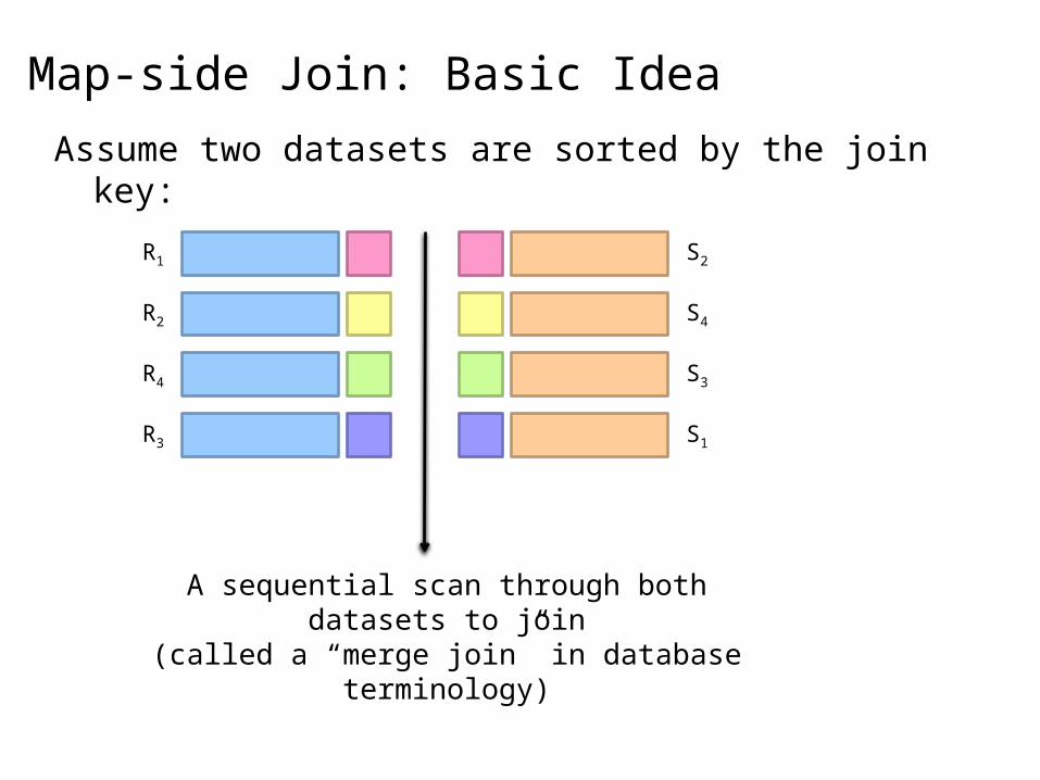
Map-side Join: Basic Idea
Assume two datasets are sorted by the join key:
R1
R2
R3
R4
S1
S2
S3
S4
A sequential scan through both datasets to join(called a “merge join” in database terminology)
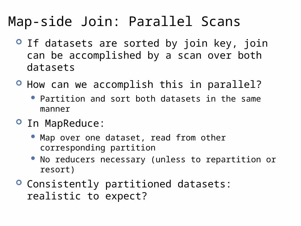
Map-side Join: Parallel Scans If datasets are sorted by join key, join can be
accomplished by a scan over both datasets
How can we accomplish this in parallel? Partition and sort both datasets in the same manner
In MapReduce: Map over one dataset, read from other corresponding partition No reducers necessary (unless to repartition or resort)
Consistently partitioned datasets: realistic to expect?

In-Memory Join Basic idea: load one dataset into memory, stream over
other dataset Works if R << S and R fits into memory Called a “hash join” in database terminology
MapReduce implementation Distribute R to all nodes Map over S, each mapper loads R in memory, hashed by join key For every tuple in S, look up join key in R No reducers, unless for regrouping or resorting tuples
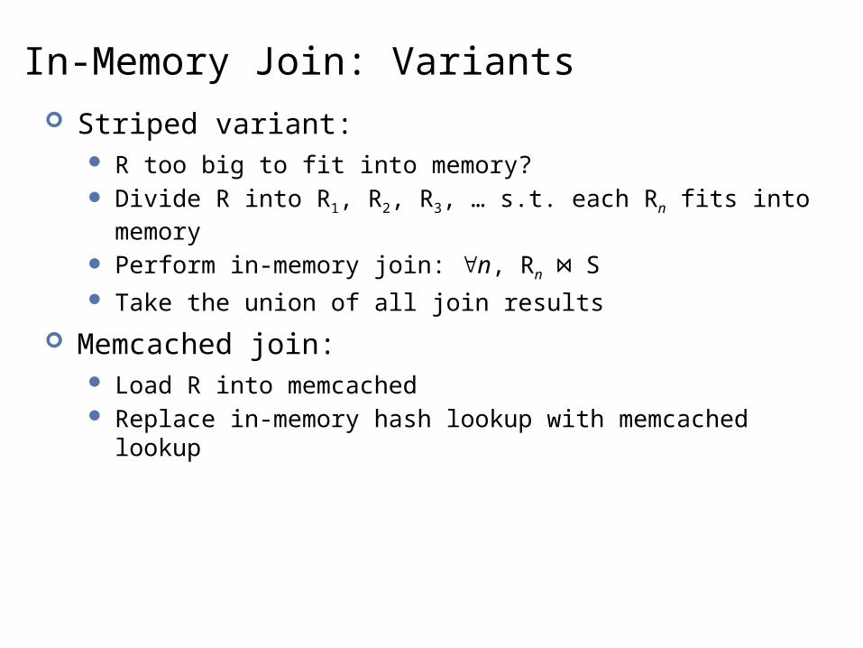
In-Memory Join: Variants Striped variant:
R too big to fit into memory? Divide R into R1, R2, R3, … s.t. each Rn fits into memory
Perform in-memory join: n, Rn S⋈ Take the union of all join results
Memcached join: Load R into memcached Replace in-memory hash lookup with memcached lookup
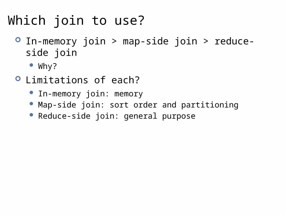
Which join to use? In-memory join > map-side join > reduce-side join
Why?
Limitations of each? In-memory join: memory Map-side join: sort order and partitioning Reduce-side join: general purpose
Key Features in Databases Common optimizations in relational databases
Reducing the amount of data to read Reducing the amount of tuples to decode Data placement Query planning and cost estimation
Same ideas can be applied to MapReduce For example, column stores in Google Dremel A few commercialized products Many research prototypes
One size does not fit all… Databases when:
You know what the question is: query optimizers work well Well-specified schema, clean data
MapReduce when: You don’t necessarily know what the question is: go brute force Exploratory data analysis Semi-structured, noisy, diverse data ETL is the insight-generation process

Graph Algorithms
Setting the stageIntroduction to MapReduceMapReduce algorithm designText retrievalManaging relational dataGraph algorithmsBeyond MapReduce

What’s a graph? G = (V,E), where
V represents the set of vertices (nodes) E represents the set of edges (links) Both vertices and edges may contain additional information
Different types of graphs: Directed vs. undirected edges Presence or absence of cycles
Graphs are everywhere: Hyperlink structure of the Web Physical structure of computers on the Internet Interstate highway system Social networks

Source: Wikipedia (Königsberg)

Some Graph Problems Finding shortest paths
Routing Internet traffic and UPS trucks
Finding minimum spanning trees Telco laying down fiber
Finding Max Flow Airline scheduling
Identify “special” nodes and communities Breaking up terrorist cells, spread of avian flu
Bipartite matching Monster.com, Match.com
And of course... PageRank

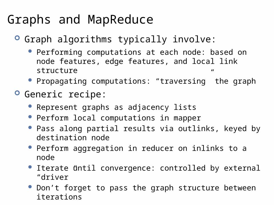
Graphs and MapReduce Graph algorithms typically involve:
Performing computations at each node: based on node features, edge features, and local link structure
Propagating computations: “traversing” the graph
Key questions: How do you represent graph data in MapReduce? How do you traverse a graph in MapReduce?

Representing Graphs G = (V, E)
Two common representations Adjacency matrix Adjacency list
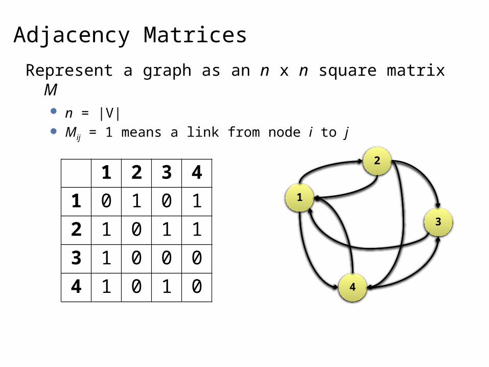
Adjacency Matrices
Represent a graph as an n x n square matrix M n = |V| Mij = 1 means a link from node i to j
1 2 3 4
1 0 1 0 1
2 1 0 1 1
3 1 0 0 0
4 1 0 1 0
1
2
3
4

Adjacency Matrices: Critique Advantages:
Amenable to mathematical manipulation Iteration over rows and columns corresponds to computations on
outlinks and inlinks
Disadvantages: Lots of zeros for sparse matrices Lots of wasted space
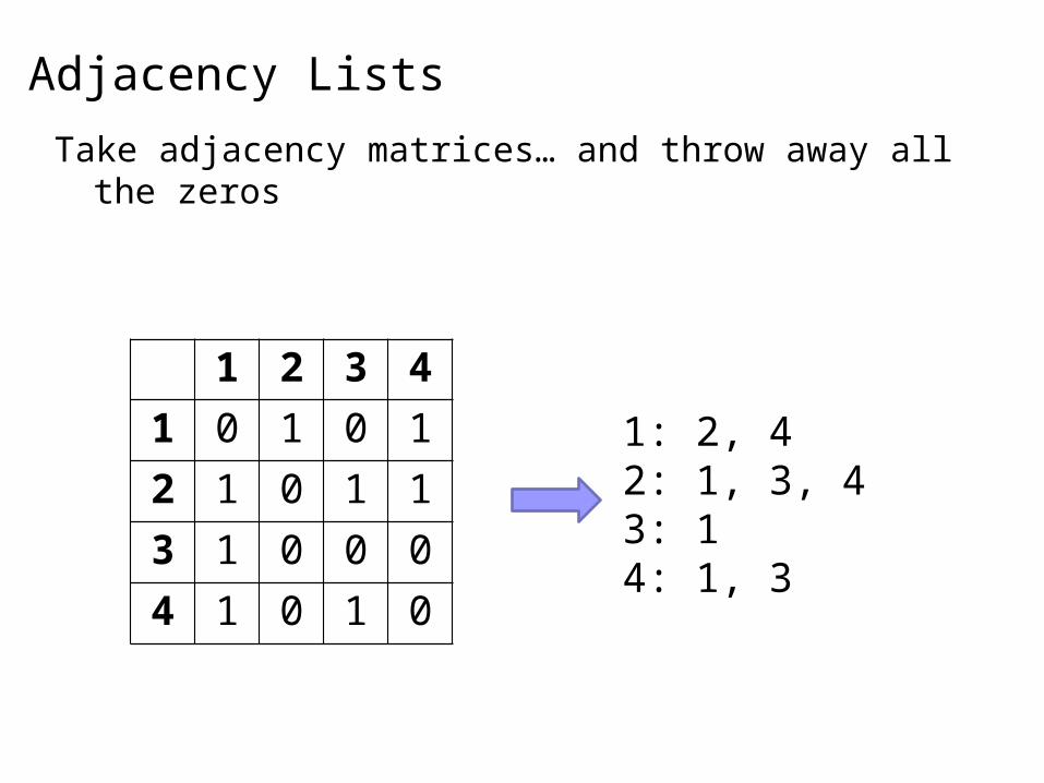
Adjacency Lists
Take adjacency matrices… and throw away all the zeros
1: 2, 42: 1, 3, 43: 14: 1, 3
1 2 3 4
1 0 1 0 1
2 1 0 1 1
3 1 0 0 0
4 1 0 1 0

Adjacency Lists: Critique Advantages:
Much more compact representation Easy to compute over outlinks
Disadvantages: Much more difficult to compute over inlinks

Single Source Shortest Path Problem: find shortest path from a source node to one or
more target nodes Shortest might also mean lowest weight or cost
First, a refresher: Dijkstra’s Algorithm

Dijkstra’s Algorithm Example
0
10
5
2 3
2
1
9
7
4 6
Example from CLR
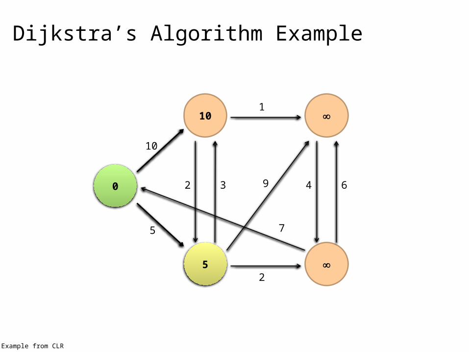
Dijkstra’s Algorithm Example
0
10
5
Example from CLR
10
5
2 3
2
1
9
7
4 6
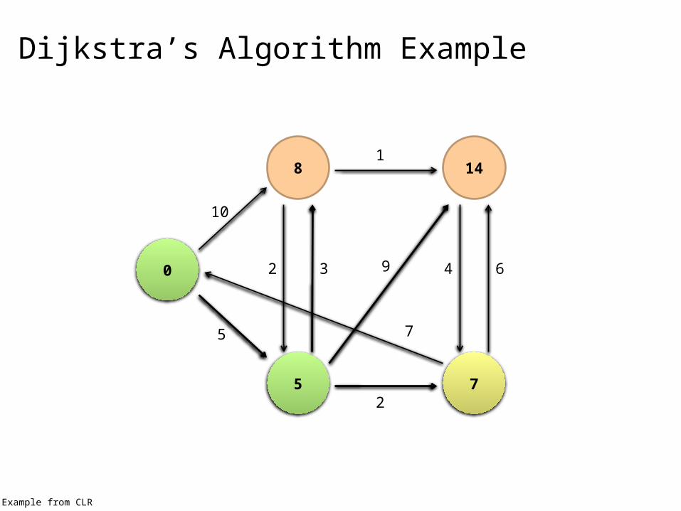
Dijkstra’s Algorithm Example
0
8
5
14
7
Example from CLR
10
5
2 3
2
1
9
7
4 6

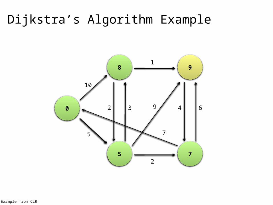
Dijkstra’s Algorithm Example
0
8
5
13
7
Example from CLR
10
5
2 3
2
1
9
7
4 6
Dijkstra’s Algorithm Example
0
8
5
9
7
1
Example from CLR
10
5
2 3
2
1
9
7
4 6

Dijkstra’s Algorithm Example
0
8
5
9
7
Example from CLR
10
5
2 3
2
1
9
7
4 6
Single Source Shortest Path Problem: find shortest path from a source node to one or
more target nodes Shortest might also mean lowest weight or cost
Single processor machine: Dijkstra’s Algorithm
MapReduce: parallel Breadth-First Search (BFS)
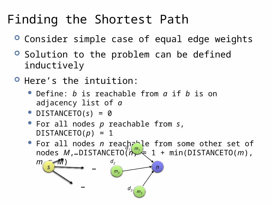
Finding the Shortest Path Consider simple case of equal edge weights
Solution to the problem can be defined inductively
Here’s the intuition: Define: b is reachable from a if b is on adjacency list of a DISTANCETO(s) = 0 For all nodes p reachable from s,
DISTANCETO(p) = 1 For all nodes n reachable from some other set of nodes M,
DISTANCETO(n) = 1 + min(DISTANCETO(m), m M)
s
m3
m2
m1
n
…
…
…
d1
d2
d3

Source: Wikipedia (Wave)

Visualizing Parallel BFS
n0
n3n2
n1
n7
n6
n5
n4
n9
n8

From Intuition to Algorithm Data representation:
Key: node n Value: d (distance from start), adjacency list (list of nodes
reachable from n) Initialization: for all nodes except for start node, d =
Mapper: m adjacency list: emit (m, d + 1)
Sort/Shuffle Groups distances by reachable nodes
Reducer: Selects minimum distance path for each reachable node Additional bookkeeping needed to keep track of actual path

Multiple Iterations Needed Each MapReduce iteration advances the “known frontier”
by one hop Subsequent iterations include more and more reachable nodes as
frontier expands Multiple iterations are needed to explore entire graph
Preserving graph structure: Problem: Where did the adjacency list go? Solution: mapper emits (n, adjacency list) as well
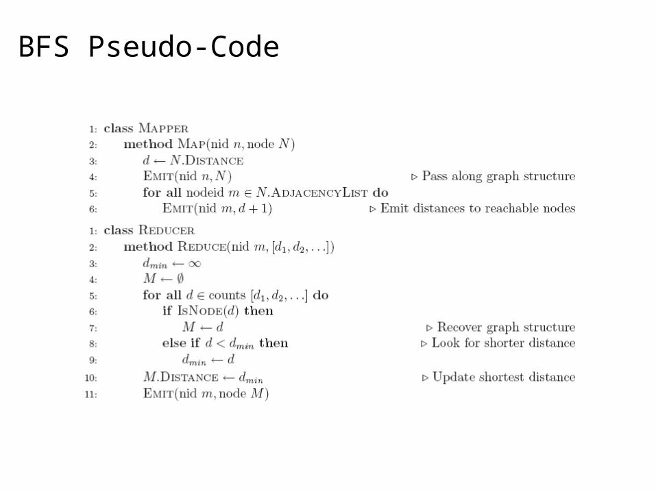
BFS Pseudo-Code

Stopping Criterion How many iterations are needed in parallel BFS (equal
edge weight case)?
When a node is first “discovered”, we’re guaranteed to have found the shortest path

Comparison to Dijkstra Dijkstra’s algorithm is more efficient
At any step it only pursues edges from the minimum-cost path inside the frontier
MapReduce explores all paths in parallel Lots of “waste” Useful work is only done at the “frontier”
Why can’t we do better using MapReduce?

Weighted Edges Now add positive weights to the edges
Simple change: adjacency list now includes a weight w for each edge In mapper, emit (m, d + wp) instead of (m, d + 1) for each node m
That’s it?

Stopping Criterion How many iterations are needed in parallel BFS (positive
edge weight case)?
When a node is first “discovered”, we’re guaranteed to have found the shortest path
Not true!

Additional Complexities
s
pq
r
search frontier
10
n1
n2
n3
n4
n5
n6 n7
n8
n9
1
11
1
1
11
1
Stopping Criterion How many iterations are needed in parallel BFS (positive
edge weight case)?
Practicalities of implementation in MapReduce
Graphs and MapReduce Graph algorithms typically involve:
Performing computations at each node: based on node features, edge features, and local link structure
Propagating computations: “traversing” the graph
Generic recipe: Represent graphs as adjacency lists Perform local computations in mapper Pass along partial results via outlinks, keyed by destination node Perform aggregation in reducer on inlinks to a node Iterate until convergence: controlled by external “driver” Don’t forget to pass the graph structure between iterations

Random Walks Over the Web Random surfer model:
User starts at a random Web page User randomly clicks on links, surfing from page to page
PageRank Characterizes the amount of time spent on any given page Mathematically, a probability distribution over pages
PageRank captures notions of page importance Correspondence to human intuition? One of thousands of features used in web search Note: query-independent
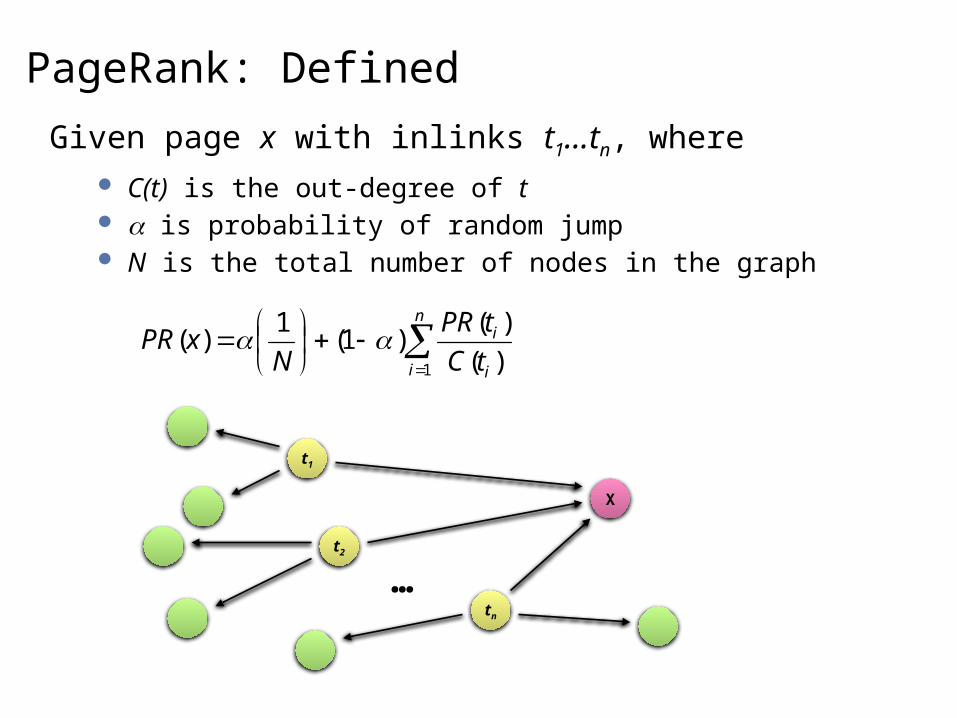
Given page x with inlinks t1…tn, where C(t) is the out-degree of t is probability of random jump N is the total number of nodes in the graph
PageRank: Defined
n
i i
i
tC
tPR
NxPR
1 )(
)()1(
1)(
X
t1
t2
tn
…
Computing PageRank Properties of PageRank
Can be computed iteratively Effects at each iteration are local
Sketch of algorithm: Start with seed PRi values
Each page distributes PRi “credit” to all pages it links to Each target page adds up “credit” from multiple in-bound links to
compute PRi+1
Iterate until values converge
Simplified PageRank First, tackle the simple case:
No random jump factor No dangling links
Then, factor in these complexities… Why do we need the random jump? Where do dangling links come from?
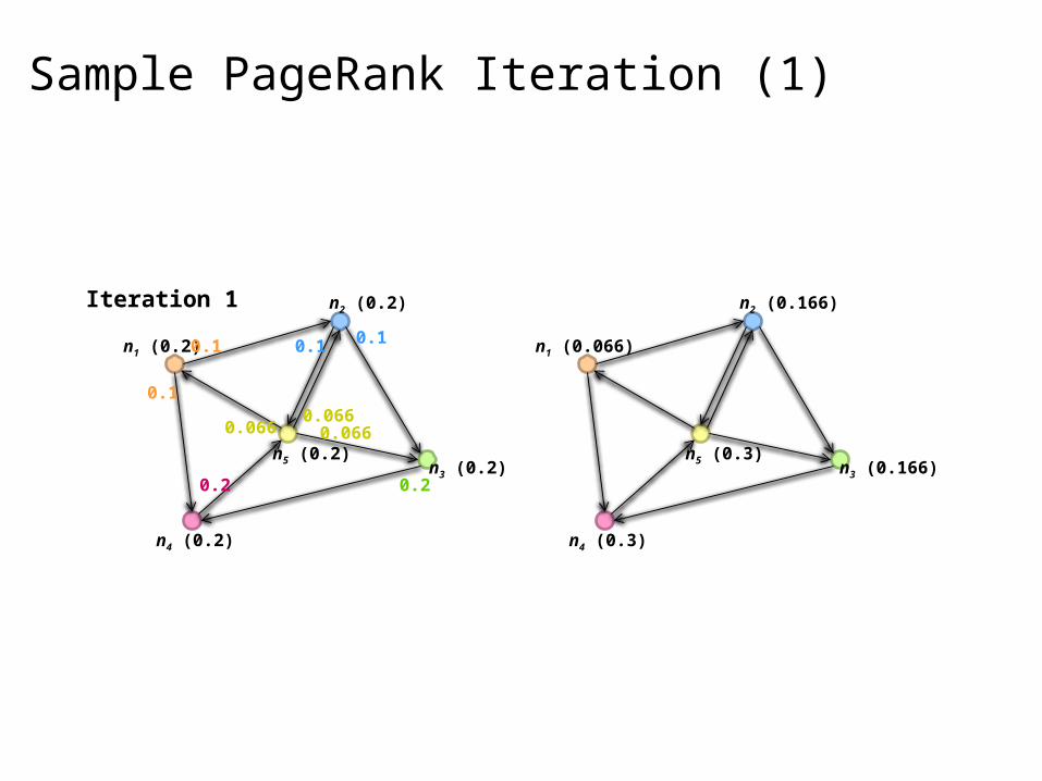
Sample PageRank Iteration (1)
n1 (0.2)
n4 (0.2)
n3 (0.2)n5 (0.2)
n2 (0.2)
0.1
0.1
0.2 0.2
0.1 0.1
0.066 0.0660.066
n1 (0.066)
n4 (0.3)
n3 (0.166)n5 (0.3)
n2 (0.166)Iteration 1

Sample PageRank Iteration (2)
n1 (0.066)
n4 (0.3)
n3 (0.166)n5 (0.3)
n2 (0.166)
0.033
0.033
0.3 0.166
0.083 0.083
0.1 0.10.1
n1 (0.1)
n4 (0.2)
n3 (0.183)n5 (0.383)
n2 (0.133)Iteration 2

PageRank in MapReduce
n5 [n1, n2, n3]n1 [n2, n4] n2 [n3, n5] n3 [n4] n4 [n5]
n2 n4 n3 n5 n1 n2 n3n4 n5
n2 n4n3 n5n1 n2 n3 n4 n5
n5 [n1, n2, n3]n1 [n2, n4] n2 [n3, n5] n3 [n4] n4 [n5]
Map
Reduce
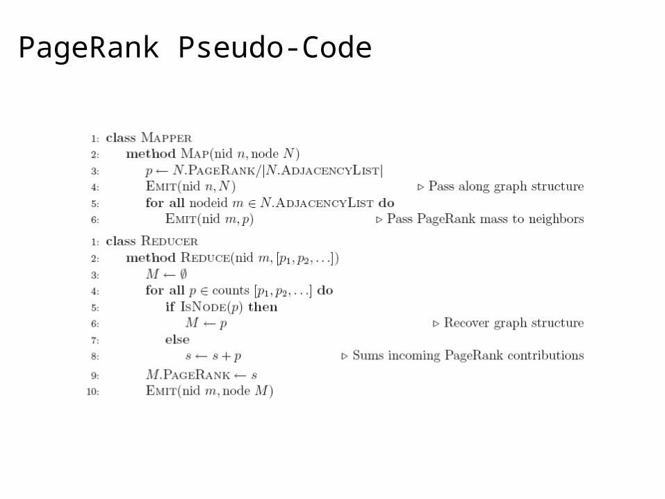
PageRank Pseudo-Code

Complete PageRank Two additional complexities
What is the proper treatment of dangling nodes? How do we factor in the random jump factor?
Solution: Second pass to redistribute “missing PageRank mass” and
account for random jumps
p is PageRank value from before, p' is updated PageRank value |G| is the number of nodes in the graph m is the missing PageRank mass
p
G
m
Gp )1(
1'

PageRank Convergence Alternative convergence criteria
Iterate until PageRank values don’t change Iterate until PageRank rankings don’t change Fixed number of iterations
Convergence for web graphs?

Beyond PageRank Link structure is important for web search
PageRank is one of many link-based features: HITS, SALSA, etc. One of many thousands of features used in ranking…
Adversarial nature of web search Link spamming Spider traps Keyword stuffing …

Efficient Graph Algorithms: Tricks In-mapper combining: efficient local aggregation
Smarter partitioning: create more opportunities for local aggregation
Schimmy: avoid shuffling the graph
Jimmy Lin and Michael Schatz. Design Patterns for Efficient Graph Algorithms in MapReduce. Proceedings of the Eighth Workshop on Mining and Learning with Graphs Workshop (MLG-2010), pages 78-85, July 2010, Washington, D.C.
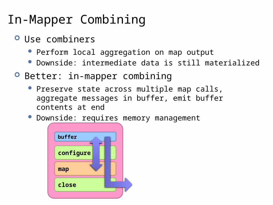
In-Mapper Combining Use combiners
Perform local aggregation on map output Downside: intermediate data is still materialized
Better: in-mapper combining Preserve state across multiple map calls, aggregate messages in
buffer, emit buffer contents at end Downside: requires memory management
configure
map
close
buffer

Better Partitioning Default: hash partitioning
Randomly assign nodes to partitions
Observation: many graphs exhibit local structure E.g., communities in social networks Better partitioning creates more opportunities for local aggregation
Unfortunately, partitioning is hard! Sometimes, chick-and-egg… But cheap heuristics sometimes available For webgraphs: range partition on domain-sorted URLs
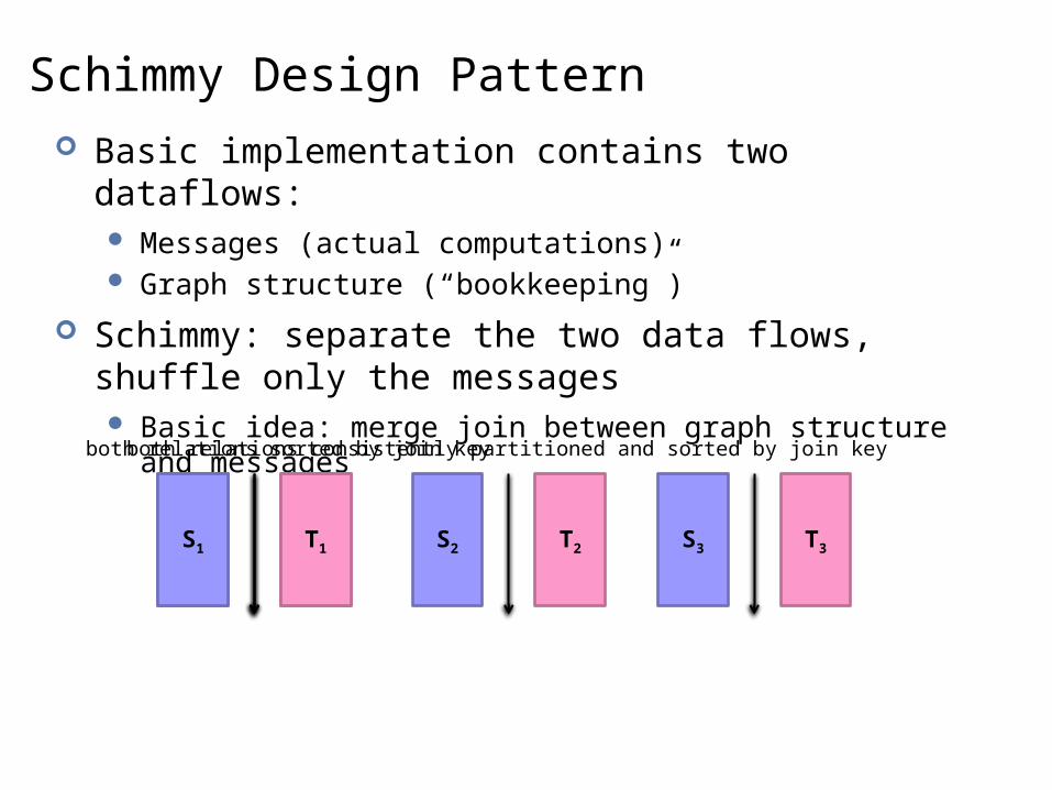
Schimmy Design Pattern Basic implementation contains two dataflows:
Messages (actual computations) Graph structure (“bookkeeping”)
Schimmy: separate the two data flows, shuffle only the messages Basic idea: merge join between graph structure and messages
S T
both relations sorted by join key
S1 T1 S2 T2 S3 T3
both relations consistently partitioned and sorted by join key

S1 T1
Do the Schimmy! Schimmy = reduce side parallel merge join between graph
structure and messages Consistent partitioning between input and intermediate data Mappers emit only messages (actual computation) Reducers read graph structure directly from HDFS
S2 T2 S3 T3
ReducerReducerReducer
intermediate data(messages)
intermediate data(messages)
intermediate data(messages)
from HDFS(graph structure)
from HDFS(graph structure)
from HDFS(graph structure)
Experiments Cluster setup:
10 workers, each 2 cores (3.2 GHz Xeon), 4GB RAM, 367 GB disk Hadoop 0.20.0 on RHELS 5.3
Dataset: First English segment of ClueWeb09 collection 50.2m web pages (1.53 TB uncompressed, 247 GB compressed) Extracted webgraph: 1.4 billion links, 7.0 GB Dataset arranged in crawl order
Setup: Measured per-iteration running time (5 iterations) 100 partitions

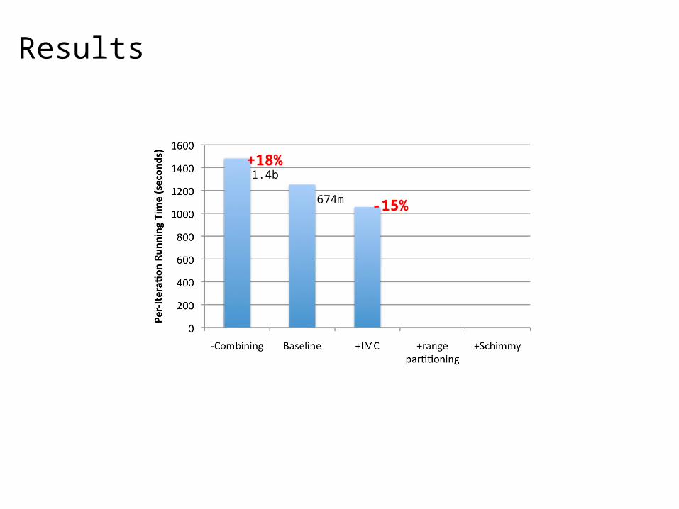
Results
“Best Practices”

Results
+18%1.4b
674m
Results
+18%
-15%
1.4b
674m
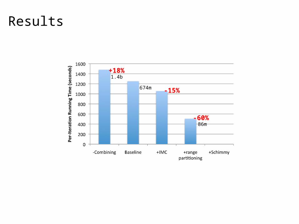
Results
+18%
-15%
-60%
1.4b
674m
86m

Results
+18%
-15%
-60%-69%
1.4b
674m
86m
Beyond MapReduce
Setting the stageIntroduction to MapReduceMapReduce algorithm designText retrievalManaging relational dataGraph algorithmsBeyond MapReduce

From GFS to Bigtable Google’s GFS is a distributed file system
Bigtable is a storage system for structured data Built on top of GFS Solves many GFS issues: real-time access, short files, short reads Serves as a source and a sink for MapReduce jobs
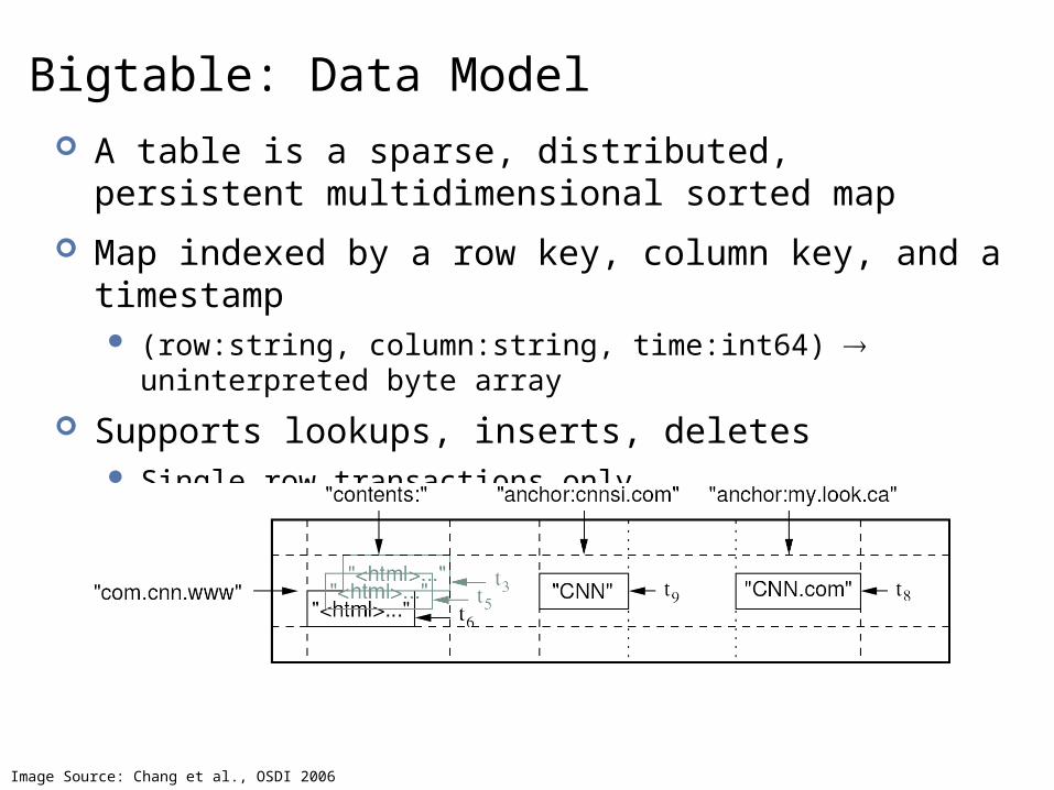
Bigtable: Data Model A table is a sparse, distributed, persistent
multidimensional sorted map
Map indexed by a row key, column key, and a timestamp (row:string, column:string, time:int64) uninterpreted byte array
Supports lookups, inserts, deletes Single row transactions only
Image Source: Chang et al., OSDI 2006

HBase
Image Source: http://www.larsgeorge.com/2009/10/hbase-architecture-101-storage.html

Source: flickr (60in3/2338247189)

Source: NY Times (6/14/2006)
The datacenter is the computer!It’s all about the right level of abstraction

Need for High-Level Languages Hadoop is great for large-data processing!
But writing Java programs for everything is verbose and slow Analysts don’t want to (or can’t) write Java
Solution: develop higher-level data processing languages Hive: HQL is like SQL Pig: Pig Latin is a dataflow language
Hive and Pig Hive: data warehousing application in Hadoop
Query language is HQL, variant of SQL Tables stored on HDFS as flat files Developed by Facebook, now open source
Pig: large-scale data processing system Scripts are written in Pig Latin, a dataflow language Developed by Yahoo!, now open source Roughly 1/3 of all Yahoo! internal jobs
Common idea: Provide higher-level language to facilitate large-data processing Higher-level language “compiles down” to Hadoop jobs

Hive: Example Hive looks similar to an SQL database
Relational join on two tables: Table of word counts from Shakespeare collection Table of word counts from the bible
Source: Material drawn from Cloudera training VM
SELECT s.word, s.freq, k.freq FROM shakespeare s JOIN bible k ON (s.word = k.word) WHERE s.freq >= 1 AND k.freq >= 1 ORDER BY s.freq DESC LIMIT 10;
the 25848 62394I 23031 8854and 19671 38985to 18038 13526of 16700 34654a 14170 8057you 12702 2720my 11297 4135in 10797 12445is 8882 6884

Hive: Behind the Scenes
SELECT s.word, s.freq, k.freq FROM shakespeare s JOIN bible k ON (s.word = k.word) WHERE s.freq >= 1 AND k.freq >= 1 ORDER BY s.freq DESC LIMIT 10;
(TOK_QUERY (TOK_FROM (TOK_JOIN (TOK_TABREF shakespeare s) (TOK_TABREF bible k) (= (. (TOK_TABLE_OR_COL s) word) (. (TOK_TABLE_OR_COL k) word)))) (TOK_INSERT (TOK_DESTINATION (TOK_DIR TOK_TMP_FILE)) (TOK_SELECT (TOK_SELEXPR (. (TOK_TABLE_OR_COL s) word)) (TOK_SELEXPR (. (TOK_TABLE_OR_COL s) freq)) (TOK_SELEXPR (. (TOK_TABLE_OR_COL k) freq))) (TOK_WHERE (AND (>= (. (TOK_TABLE_OR_COL s) freq) 1) (>= (. (TOK_TABLE_OR_COL k) freq) 1))) (TOK_ORDERBY (TOK_TABSORTCOLNAMEDESC (. (TOK_TABLE_OR_COL s) freq))) (TOK_LIMIT 10)))
(one or more of MapReduce jobs)
(Abstract Syntax Tree)
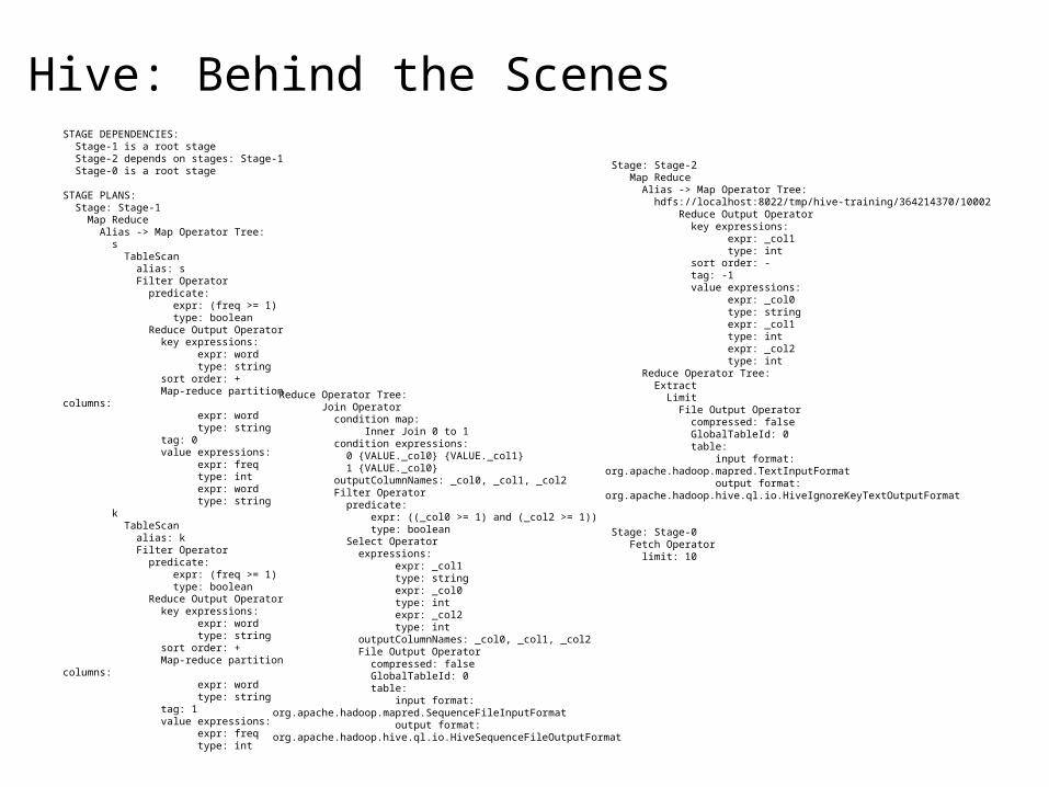
Hive: Behind the ScenesSTAGE DEPENDENCIES: Stage-1 is a root stage Stage-2 depends on stages: Stage-1 Stage-0 is a root stage
STAGE PLANS: Stage: Stage-1 Map Reduce Alias -> Map Operator Tree: s TableScan alias: s Filter Operator predicate: expr: (freq >= 1) type: boolean Reduce Output Operator key expressions: expr: word type: string sort order: + Map-reduce partition columns: expr: word type: string tag: 0 value expressions: expr: freq type: int expr: word type: string k TableScan alias: k Filter Operator predicate: expr: (freq >= 1) type: boolean Reduce Output Operator key expressions: expr: word type: string sort order: + Map-reduce partition columns: expr: word type: string tag: 1 value expressions: expr: freq type: int
Reduce Operator Tree: Join Operator condition map: Inner Join 0 to 1 condition expressions: 0 {VALUE._col0} {VALUE._col1} 1 {VALUE._col0} outputColumnNames: _col0, _col1, _col2 Filter Operator predicate: expr: ((_col0 >= 1) and (_col2 >= 1)) type: boolean Select Operator expressions: expr: _col1 type: string expr: _col0 type: int expr: _col2 type: int outputColumnNames: _col0, _col1, _col2 File Output Operator compressed: false GlobalTableId: 0 table: input format: org.apache.hadoop.mapred.SequenceFileInputFormat output format: org.apache.hadoop.hive.ql.io.HiveSequenceFileOutputFormat
Stage: Stage-2 Map Reduce Alias -> Map Operator Tree: hdfs://localhost:8022/tmp/hive-training/364214370/10002 Reduce Output Operator key expressions: expr: _col1 type: int sort order: - tag: -1 value expressions: expr: _col0 type: string expr: _col1 type: int expr: _col2 type: int Reduce Operator Tree: Extract Limit File Output Operator compressed: false GlobalTableId: 0 table: input format: org.apache.hadoop.mapred.TextInputFormat output format: org.apache.hadoop.hive.ql.io.HiveIgnoreKeyTextOutputFormat
Stage: Stage-0 Fetch Operator limit: 10

Pig: Example
User Url Time
Amy cnn.com 8:00
Amy bbc.com 10:00
Amy flickr.com 10:05
Fred cnn.com 12:00
Url Category PageRank
cnn.com News 0.9
bbc.com News 0.8
flickr.com Photos 0.7
espn.com Sports 0.9
Visits Url Info
Task: Find the top 10 most visited pages in each category
Pig Slides adapted from Olston et al. (SIGMOD 2008)

Pig Query Plan
Load VisitsLoad Visits
Group by urlGroup by url
Foreach urlgenerate count
Foreach urlgenerate count Load Url InfoLoad Url Info
Join on urlJoin on url
Group by categoryGroup by category
Foreach categorygenerate top10(urls)
Foreach categorygenerate top10(urls)
Pig Slides adapted from Olston et al. (SIGMOD 2008)

Pig Script
visits = load ‘/data/visits’ as (user, url, time);
gVisits = group visits by url;
visitCounts = foreach gVisits generate url, count(visits);
urlInfo = load ‘/data/urlInfo’ as (url, category, pRank);
visitCounts = join visitCounts by url, urlInfo by url;
gCategories = group visitCounts by category;
topUrls = foreach gCategories generate top(visitCounts,10);
store topUrls into ‘/data/topUrls’;
Pig Slides adapted from Olston et al. (SIGMOD 2008)

Load VisitsLoad Visits
Group by urlGroup by url
Foreach urlgenerate count
Foreach urlgenerate count Load Url InfoLoad Url Info
Join on urlJoin on url
Group by categoryGroup by category
Foreach categorygenerate top10(urls)
Foreach categorygenerate top10(urls)
Pig Script in Hadoop
Map1
Reduce1Map2
Reduce2
Map3
Reduce3
Pig Slides adapted from Olston et al. (SIGMOD 2008)

Different Programming Models Multitude of MapReduce hybrids, variants, etc.
Mostly research prototypes A few commercial companies
Dryad/DryadLINQ (Microsoft)

Emerging Themes Continuing quest for alternative programming models
Batch vs. real-time data processing
Continuing quest for better implementations
MapReduce as yet another tool
Growth of the Hadoop ecosystem
Evolving role of MapReduce and parallel databases

Questions?


