Large Eddy Simulation of Turbulent Flow Past a Bluff Body using OpenFOAM
A Thesis Presented
By
David Joseph Hensel
To
The Department of Mechanical and Industrial Engineering
in partial fulfillment of the requirements for the degree of
Master of Science
in
Mechanical Engineering
Northeastern University Boston, Massachusetts
August 2014
Large Eddy Simulation of Turbulent Flow Past a Bluff Body using OpenFOAM
M.S. Defense by
David Hensel
Tuesday, July 29th 2014, 12:00pm – 1:00pm, 09 Forsythe Northeastern University, 2014
Abstract Numerical simulation of a turbulent bluff-‐body flow is conducted using large eddy simulation (LES). The open source CFD software package, OpenFOAM, is employed to solve the LES filtered transport equations governing the three-‐dimensional incompressible flow in the wake of the body. This work is motivated by the importance of bluff-‐body flows, for example, in flame stabilization in industrial combustors and burners, as well as in aerodynamics applications. The focus of the study is on the proper generation of turbulence at the inlet boundary. Standard boundary conditions available in OpenFOAM are not sufficient for providing an accurate turbulent inlet condition without modification of the bluff geometry. An improved method describing the inflow boundary condition is developed based on the existing OpenFOAM mapping-‐type boundary condition. In this method, the boundary condition scales the standard deviation and mean value of the velocity field onto the prescribed values provided by the experimental data. The method is implemented in OpenFOAM and employed in LES prediction of a turbulent bluff-‐body flow, studied in the experiments of the Clean Combustion Research Group at the University of Sydney. The LES results show favorable agreements with the experimental data.
Thesis Committee Members
Prof. Reza Sheikhi
Contents
Table of Figures .......................................................................................................................................................................... 1
1. Introduction ........................................................................................................................................................................ 2
2. Formulation ........................................................................................................................................................................ 3
3. Simulation ............................................................................................................................................................................ 6
3.1. OpenFOAM ................................................................................................................................................................. 6
3.2. Numerical Specification ....................................................................................................................................... 6
3.3. Grid ............................................................................................................................................................................... 8
3.4. Turbulent Inlet Boundary Condition ........................................................................................................... 10
3.4.1. Scaling Method ................................................................................................................................................. 11
4. Results ................................................................................................................................................................................ 13
5. Summary and Concluding Remarks ...................................................................................................................... 22
References .................................................................................................................................................................................. 24
1
Table of Figures
Figure 1: Bluff Body Schematic ............................................................................................................................................................ 7
Figure 2: Computational Domain Representation using ParaView (dimensions in millimeters) .......................... 9
Figure 3: Resolution of Circular Jet (37 cells) ................................................................................................................................ 9
Figure 4: Instantaneous Streamwise Filtered Velocity Iso-‐surfaces (clipped by X-‐Y plane) ................................. 14
Figure 5: Magnitude of Instantaneous Vorticity Iso-‐surfaces (clipped by X-‐Y plane) .............................................. 15
Figure 6: Line Integral Convolution of Streamwise Filtered Velocity in Bluff Region, X-‐Y Plane ........................ 15
Figure 7: LES filtered Streamwise Velocity Contours Predicted by the Smagorinsky Model. ............................... 16
Figure 8: LES filtered Streamwise Velocity Contours Predicted by the Dynamic One Equation Model. .......... 17
Figure 9: Radial Profiles of the Mean and Resolved RMS Streamwise Velocity (x=0.003, 0.01, 0.02 [m]). ..... 18
Figure 10: Radial Profiles of the Mean and Resolved RMS Streamwise Velocity (x=0.03, 0.04, 0.05 [m]). ..... 19
Figure 11: Radial Profiles of the Mean and Resolved RMS Streamwise Velocity (x=0.06 [m]). ........................... 20
Figure 12: Radial Profiles of the Mean Radial Velocity (x=0.003, 0.01 [m]). ................................................................ 20
Figure 13: Radial Profiles of the Mean Radial Velocity (x = 0.02, 0.03, 0.04[m]). ....................................................... 21
Figure 14: Radial Profiles of the Mean Radial Velocity (x = 0.05, 0.06[m]). .................................................................. 22

2
1. Introduction
Approaches for simulations of turbulent reacting flows can be divided into three categories: direct
numerical simulation (DNS), large eddy simulation (LES), and Reynolds averaged Navier-‐Stokes
simulation (RANS). DNS provides the most detailed predictions and is a useful tool for the studying
the physics of turbulent flows; however, the large number of grid points required makes DNS of
engineering-‐type problems prohibitively expensive in the foreseeable future [1]. Solutions of
RANS equations, on the other hand, are now widely used in engineering applications to predict flow
in fairly complex configurations. This approach, however, suffers from one principal shortcoming;
the fact that the turbulence model must represent a very wide range of scales reduces its reliability
as an accurate predictive tool. Among the three approaches, LES is an attractive simulation method
as it provides a compromise between accuracy and computational cost. LES is known to be the
optimal means of capturing the detailed, unsteady physics of turbulent flows. [2]
The basic idea in LES is to resolve the large-‐scale turbulent motions and to model the small-‐scale
motions, which are more universal. This idea can be explained in terms of the energy cascade
concept. The turbulent energy is transferred from large-‐scale motions to smaller scales, until finally
dissipated into heat by viscosity at the molecular level. According to Kolmogorov’s hypotheses, a
scale separation exists within the energy cascade where turbulent energy is produced in the largest
scales, transferred to decreasing scales by the energy cascade within the inertial subrange, and
dissipated through viscosity at the smallest scales. In LES, it is essential to resolve about 80% of the
turbulent energy of the large scales while representing about 20% transferred to small scales using
a subgrid scale (SGS) model. RANS has an inherent shortcoming since it averages over all turbulent
scales and thus, provides a time-‐averaged field; however, LES provides time-‐dependent fields,
which offers improved accuracy in predicting unsteady turbulent motions. The benefit of LES is
evident in flows where vortex shedding and unsteady separation are significant [3].

3
In the present study, LES prediction of turbulent flow past a bluff body is performed. This study is
motivated by the importance of bluff-‐body flows within various combustion applications. In this
context, bluff bodies provide a simple geometry to study recirculation zones that help stabilize the
flame. The purpose of this study is to validate the hydrodynamic solution for the non-‐reacting bluff
body flow studied experimentally by the Clean Combustion Research Group at the University of
Sydney [4]. Previous studies of this geometry include works of Drozda [5] and Drozda et al. [6],
which involve LES based on filtered density function (FDF) methodology for prediction of non-‐
reacting and reacting flows in this configuration.
In this study, we use the OpenFOAM software package to conduct simulation of the same
configuration. Simulation of flows around bluff bodies using OpenFOAM has been the subject of
several studies. Lysenko et al. [7] studied turbulent flow around triangular bluff bodies, and
compares results from OpenFOAM with ANSYS Fluent. Salvador et al. [8] included a non-‐reacting
case in their study of a premixed reacting flame using OpenFOAM. An important issue in accurate
simulation of turbulent flows is proper generation of turbulent inlet boundary conditions, where
various statistics are not only time varying, but also physically representative of turbulent flow.
Several methods have been developed to address this boundary condition, including the use of pre-‐
compiled data from a precursor study, generating synthetic turbulence, or turbulence mapping
methods [9]. Volavy et al. [10] provided a comparison of a uniform inlet velocity profile, with that
of a mapped turbulent inlet, and demonstrated the need for proper turbulent inlet for flows over a
reversed step. In this study, we developed an improved inflow boundary condition based on the
OpenFOAM mapping-‐type boundary condition, as discussed in Section 3.4.
2. Formulation
The basic equations governing incompressible isothermal turbulent flows are the conservation of
mass and momentum by describing variation of transport variables in space 𝑥!(𝑖 = 1,2,3) and
4
time 𝑡. The transport variables used are fluid density 𝜌(𝑥, 𝑡), pressure 𝑝(𝑥, 𝑡), and the velocity
vector 𝑢!(𝑥! , 𝑡) (𝑖 = 1,2,3).
𝜕𝜌𝜕𝑡+𝜕𝜌𝑢!𝜕𝑥!
= 0 (1)
𝜕𝜌𝑢!𝜕𝑡
+𝜕𝜌𝑢!𝑢!𝜕𝑥!
= −𝜕𝑝𝜕𝑥!
+ 𝜌𝜈𝜕!𝑢!𝜕𝑥!𝜕𝑥!
(2)
where 𝜈 denotes the kinematic viscosity.
LES uses a spatial filtering method which is essentially the convolution integral over the entire
volume [3] ,
𝑢 𝑥! , 𝑡 = 𝐺 𝑟! , 𝑥! 𝑢(𝑥! − 𝑟! , 𝑡)𝑑𝑟!
!!
!! (3)
where G is a filter that satisfies the normalization condition
𝐺 𝑟! , 𝑥! 𝑑𝑟! = 1 (4)
and U is any function of space and time and denotes the filtered field variables.
As a result of LES filtering we obtain a residual field defined as
𝑢′ 𝑥! , 𝑡 ≡ 𝑢 𝑥! , 𝑡 − 𝑢 𝑥! , 𝑡 (5)
We thus have
𝑢 𝑥! , 𝑡 = 𝑢 𝑥! , 𝑡 + 𝑢′ 𝑥! , 𝑡 (6)
The filtered form of the governing equation is obtained by applying the filtering operation to Eqs.
(1) and (2).
𝜕𝜌𝜕𝑡+𝜕𝜌 𝑢!𝜕𝑥!
= 0 (7)
𝜕𝜌 𝑢!𝜕𝑡
+𝜕𝜌 𝑢!𝑢!𝜕𝑥!
= −𝜕 𝑝𝜕𝑥!
+ 𝜌𝜈𝜕! 𝑢!𝜕𝑥!𝜕𝑥!
(8)
5
We can decompose the second term on the left side of Eq. (8) as
𝜕𝜌 𝑢!𝑢!𝜕𝑥!
=𝜕𝜌 𝑢! + 𝑢!! 𝑢! + 𝑢!!
𝜕𝑥!=𝜕𝜌 𝑢! 𝑢!
𝜕𝑥!+𝜕𝜌𝜏!"!
𝜕𝑥! (9)
where 𝜏!"! = 𝑢!𝑢! − 𝑢! 𝑢! and is defined as the residual or SGS stress tensor. The residual
stress tensor is unclosed and must be modeled, since we have no representation of 𝑢!𝑢! available
by the governing equations. The residual kinetic energy is defined as
𝑘! ≡12𝜏!!! (10)
The residual kinetic energy is related to the isotropic part of the residual stress tensor. The
anisotropic component of the residual stress tensor is responsible for momentum transport.
𝜏!"! ≡ 𝜏!!! −23𝑘!𝛿!" (11)
where 𝛿!" is the Kronecker delta. The isotropic component can be combined into a modified filtered
pressure
𝑝! ≡ 𝑝 +23𝜌𝑘! (12)
The resulting filtered momentum equation is obtained as
𝜕 𝑢!𝜕𝑡
+𝜕 𝑢! 𝑢!𝜕𝑥!
= 𝜈𝜕! 𝑢!𝜕𝑥!𝜕𝑥!
−𝜕𝜏!"!
𝜕𝑥!−1𝜌𝜕 𝑝!𝜕𝑥!
(13)
The LES closure problem is due to the residual stress tensor. The SGS modeling of this stress has
been addressed in many investigations and several closures have been developed; examples
include the Smagorinsky and dynamic models [3].
6
3. Simulation
3.1. OpenFOAM
In this study, we use the OpenFOAM software package to perform the computational fluid dynamics
(CFD) simulation of the flow past the bluff body. OpenFOAM has been offered as open-‐source
software since 2004 [11]. The software contains a full suite of numerical methods, solvers,
boundary conditions, meshing, and plug-‐ins for third party post-‐processing using the application
ParaView (also open-‐source). In addition to the numerical capabilities, OpenFOAM provides built-‐
in parallelism for high-‐performance computing using Message Passing Interface (MPI), There are
several studies showing good scalability of OpenFOAM on various computing platforms [12];
however, the scalability of the simulation varies based on the details of the numerics.
3.2. Numerical Specification
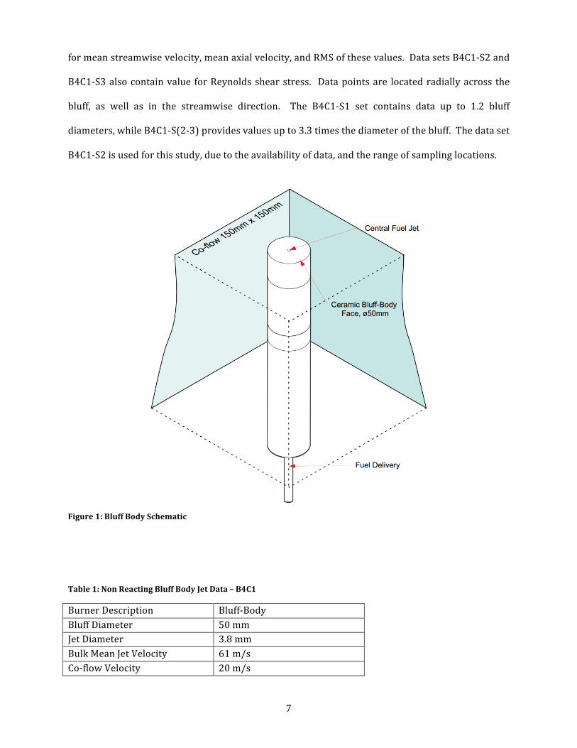
The data used for this analysis is provided by the experimental studies of a flat faced, cylindrical
bluff body axially centered in a stream of air (co-‐flow), performed at the University of Sydney. The
bluff body contains a fuel jet at the center. Details of the geometry are shown in Figure 1, and the
configuration parameters are provided in
Table 1. Additional data for this geometry is available from the Clean Combustion Research Group
website [4].
The boundary conditions applied in the present simulations are generally consistent with the
experimental setup at the University of Sydney; zero-‐gradient velocity and pressure are applied at
the exit plane of the domain, and the sides (co-‐flow) specified as symmetry planes to provide the
representation of a wind tunnel. The bluff face is modeled by specifying zero velocity, and zero-‐
gradient pressure.
In this study, we select the non-‐reacting bluff body jet configuration B4C1. Three sets of data are
available for this configuration, denoted as B4C1-‐S(1-‐3). Each set contains data at various points
7
for mean streamwise velocity, mean axial velocity, and RMS of these values. Data sets B4C1-‐S2 and
B4C1-‐S3 also contain value for Reynolds shear stress. Data points are located radially across the
bluff, as well as in the streamwise direction. The B4C1-‐S1 set contains data up to 1.2 bluff
diameters, while B4C1-‐S(2-‐3) provides values up to 3.3 times the diameter of the bluff. The data set
B4C1-‐S2 is used for this study, due to the availability of data, and the range of sampling locations.
Figure 1: Bluff Body Schematic
Table 1: Non Reacting Bluff Body Jet Data – B4C1
Burner Description Bluff-‐Body Bluff Diameter 50 mm Jet Diameter 3.8 mm Bulk Mean Jet Velocity 61 m/s Co-‐flow Velocity 20 m/s
8
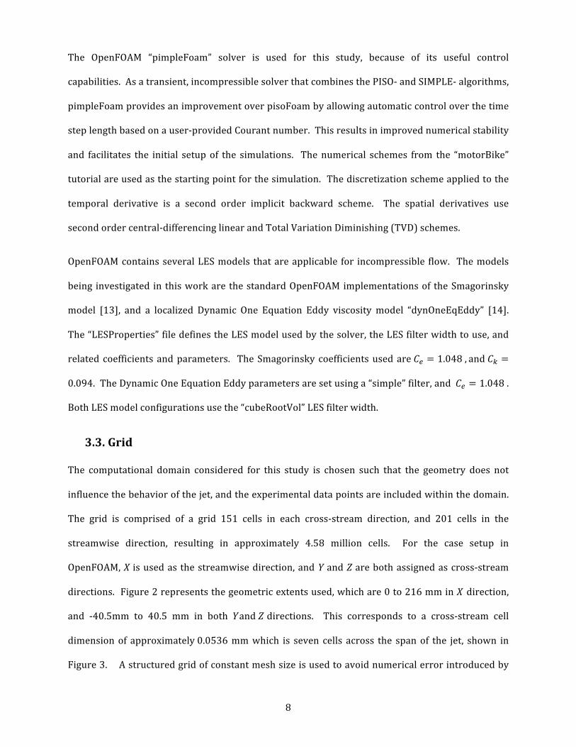
The OpenFOAM “pimpleFoam” solver is used for this study, because of its useful control
capabilities. As a transient, incompressible solver that combines the PISO-‐ and SIMPLE-‐ algorithms,
pimpleFoam provides an improvement over pisoFoam by allowing automatic control over the time
step length based on a user-‐provided Courant number. This results in improved numerical stability
and facilitates the initial setup of the simulations. The numerical schemes from the “motorBike”
tutorial are used as the starting point for the simulation. The discretization scheme applied to the
temporal derivative is a second order implicit backward scheme. The spatial derivatives use
second order central-‐differencing linear and Total Variation Diminishing (TVD) schemes.
OpenFOAM contains several LES models that are applicable for incompressible flow. The models
being investigated in this work are the standard OpenFOAM implementations of the Smagorinsky
model [13], and a localized Dynamic One Equation Eddy viscosity model “dynOneEqEddy” [14].
The “LESProperties” file defines the LES model used by the solver, the LES filter width to use, and
related coefficients and parameters. The Smagorinsky coefficients used are 𝐶! = 1.048 , and 𝐶! =
0.094. The Dynamic One Equation Eddy parameters are set using a “simple” filter, and 𝐶! = 1.048 .
Both LES model configurations use the “cubeRootVol” LES filter width.
3.3. Grid
The computational domain considered for this study is chosen such that the geometry does not
influence the behavior of the jet, and the experimental data points are included within the domain.
The grid is comprised of a grid 151 cells in each cross-‐stream direction, and 201 cells in the
streamwise direction, resulting in approximately 4.58 million cells. For the case setup in
OpenFOAM, X is used as the streamwise direction, and Y and Z are both assigned as cross-‐stream
directions. Figure 2 represents the geometric extents used, which are 0 to 216 mm in 𝑋 direction,
and -‐40.5mm to 40.5 mm in both 𝑌and 𝑍 directions. This corresponds to a cross-‐stream cell
dimension of approximately 0.0536 mm which is seven cells across the span of the jet, shown in
Figure 3. A structured grid of constant mesh size is used to avoid numerical error introduced by

9
non-‐orthogonality, as well as LES filtering commutation error. A three-‐dimensional, structured
mesh is used to simulate the inherently three-‐dimensional nature of turbulent fluid flow variables.
Figure 2: Computational Domain Representation using ParaView (dimensions in millimeters)
Figure 3: Resolution of Circular Jet (37 cells)
The mesh for this study is generated using the OpenFOAM meshing utility blockMesh. The overall
geometry is specified as a single block rectangular prism with eight vertices, extending in the

10
positive X direction from the Y-‐Z plane, and centered about the origin. Each side of the block is
assigned to a named collection of cells on the mesh boundary called a “patch.”
A mesh utility topoSet is used to create groups of cells called “cellSets,” based on a specified
geometric condition such as cylinders of diameter Dbluff and Djet corresponding to bluff and jet
nozzle, respectively. These groups of cells are used to determine which cells lie within the specified
geometry, and are coincident with the boundary faces of the “inlet” patch. From this information,
groups of faces called “faceSets” are used to create patches to represent the bluff geometry on the
inlet plane. The createPatch utility is used to make the “jet” and “bluff” patches, by reassigning faces
from the “inlet” patch using “faceSets.” This results in a well-‐defined circular geometry for the jet
and the bluff. The resulting “jet” patch area is approximately 4% larger than the actual surface area
of the jet, and the “bluff” patch is approximately 1% less than the actual surface area of the bluff.
This case was modeled without using a physical representation of the bluff burner geometry, but
rather placing this geometry specification as a “patch” on the mesh boundary.
3.4. Turbulent Inlet Boundary Condition
As described by Gabor and Baba-‐Ahmadi [15], a turbulent inlet boundary condition should remain
generic and allow turbulent properties to be specified easily, so the boundary condition is
applicable for a variety of flow conditions. There are several methods to describe a turbulent inlet
flow boundary condition properly. One of these is generation of synthetic turbulence, by means of a
forcing frequency derived from characteristic flow parameters. This method can provide a very
precise description of the boundary condition for the specific flow configuration; however, it is case
dependent and not trivial to derive. Another method involves a precursor study where turbulent
fields are created and stored for use as a pre-‐defined, time-‐dependent turbulence library. This
method may be computationally expensive to generate, but provides a reusable boundary
description for the specific flow conditions generated. A promising method is to simulate
turbulence by creating an isolated sub-‐domain with cyclic boundaries. This essentially creates an
infinitely long domain, which allows generation of fully developed turbulent flow, typically wall

11
bounded, channel or pipe flow. This requires additional computational expense, as these cells are
not a part of the computational domain of interest, and provide no other use other than generating
inlet turbulence. The resulting turbulence created by the cyclic boundary method reasonably
represents turbulent flow, which is not simply the collection of random signals, but rather a
collection of coherent turbulent structures governed by transport equations (Eqs. (1) and (2)). A
modification to this method is the mapped turbulent sub-‐domain, which involves providing the
sampling plane within the computational domain of interest, thereby reducing the additional cells
required for generating turbulence. This method is implemented in OpenFOAM, as the “mapped”
boundary condition, and provides control by using an optional method to scale the sampled field to
a prescribed mean value. The mapping method has shown to be successful for channel flow [9], and
provides a simple, yet accurate description of turbulent flow. The boundary condition used in this
study is based on the mapped boundary condition in OpenFOAM.
3.4.1. Scaling Method
The premise of the mapped boundary condition is that the faces of a boundary patch are projected
onto an arbitrary plane within the computational domain. These values are then collected into a
list, on which scaling operations are then performed. Finally, these scaled values are reassigned to
their corresponding boundary faces. The OpenFOAM mapped boundary condition scales the mean
velocity of the sample by shifting all the values, or by multiplying the sampled field by a scale factor,
depending on the relation between the local sampled average and the prescribed value. The scaling
method uses the prescribed value divided by a calculated sample mean value to develop a scale
factor. When a multiplier scales the velocity, that multiplier also scales the standard deviation of
the field. This is undesirable when the sampled field mean value is significantly different from the
prescribed mean value. For the bluff-‐body flow the sample velocity shall always be less than or
equal to the inlet velocity for a jet expanding into a slower moving co-‐flow. This limitation is
addressed by the alternative scaling method described in this work, where the standard deviation is
controlled by scaling the sampled field to a prescribed value. This sampling results in better

12
agreement of filtered velocity with the data. To match the RMS values, the first step is to calculate
the standard deviation of the sampled field. Then we calculate a scaling factor by dividing the
desired standard deviation by the sampled standard deviation.
𝛾 =𝜎!"#$%"&'#(𝜎!"#$%&'
(14)
where 𝜎 denotes the standard deviation. Next, each value of the sampled field is multiplied by the
scaling factor to create a scaled field.
𝑢 !"#$%& = 𝛾 𝑢 !"#$%&' (15)
Now we calculate the “mean shift” difference between the mean value of the scaled field and the
desired mean value
𝛽 = 𝑢 !"#$%"!"#$ − 𝑢 !"#$%& (16)
where denotes the local mean value calculated from the sampled points. Finally, add the “mean
shift” to each value of the scaled field to obtain the final field that has been scaled in both mean
value and standard deviation.
𝑢 !"#$% = 𝑢 !"#$%& + 𝛽 (17)
This scaling method is applied to each component of the velocity for the boundary condition used in
this research. The bulk mean velocity and fluctuations from the experimental data initial conditions
are used to define the boundary condition for both the jet and co-‐flow. This method aims to
generate realistic turbulence by sampling existing fluctuations from the internal domain, rather
than generating a synthetic perturbed inlet. In comparison to the standard boundary condition,
this method provides additional control over the second order statistics. The current
implementation scales the distribution of each vector component to a prescribed standard
deviation and mean value. The intent of this mapping/scaling boundary condition is to provide the
bulk mean statistical description of the jet.

13
4. Results
The computational work done for this study is performed using the Texas Advanced Computing
Center (TACC) Stampede Supercomputer located at the University of Texas at Austin. Simulations
are also performed using Northeastern University’s Discovery Cluster at the Massachusetts Green
High Performance Computing Center (MGHPCC). OpenFOAM 2.3.0 is used at both facilities, with
modified solvers and boundary conditions.
The simulation is compared against the non-‐reacting experimental data set B4C1-‐S2. The following
figures are plotted using time-‐averaged results, which is averaged about the angular direction to
provide results in a consistent format with that of the experiment. The results compare two
different LES models from OpenFOAM with all other case parameters held constant. Figure 4 and
Figure 5 demonstrate the turbulent nature of the bluff body flow, showing instantaneous iso-‐
surfaces of streamwise filtered velocity, and magnitude of vorticity, respectively. The time-‐
averaged streamwise velocity shown in Figure 6 displays the recirculation zone of the bluff body,
with an inner and outer vortex structure visible by Line Integral Convolution.
A limitation of the mapping boundary condition is the inability to define the profile of the sampled
field; as a result, a single value must be specified. The mean values calculated from the initial
conditions do not provide good agreement with the data when used with the mapped boundary
condition. During initial studies, the mean velocity was under-‐predicted and the turbulent
fluctuations were over-‐predicted using both LES models. To address this issue, the mean value and
fluctuations are modified to maintain closer agreement with the experimental data. The mapped
turbulent inlet boundary condition is specified to maintain a scaled mean velocity of 70.76 m/s,
which corresponds to the centerline velocity specified in the initial conditions. The scaled sampled
standard deviation is set to maintain approximately 1% of the scaled mean velocity. The velocity
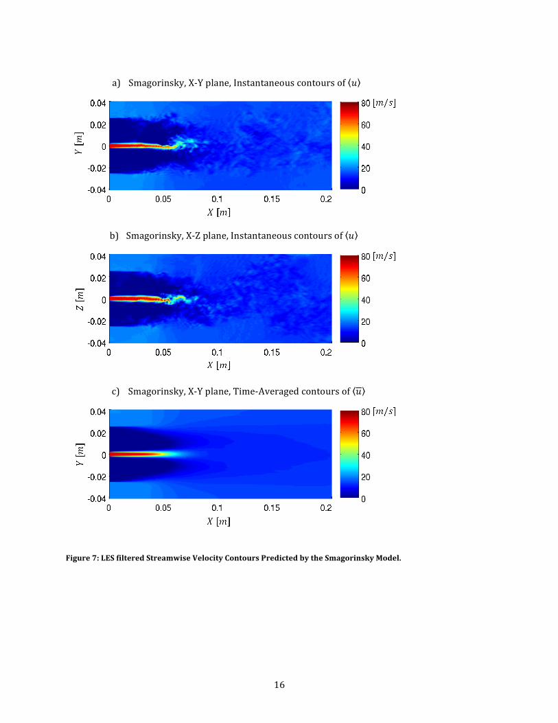
contours predicted by the Smagorinsky model shown in Figure 7 demonstrate the longer, less
turbulent jet than that shown in Figure 8 predicted by the Dynamic One Equation model. The

14
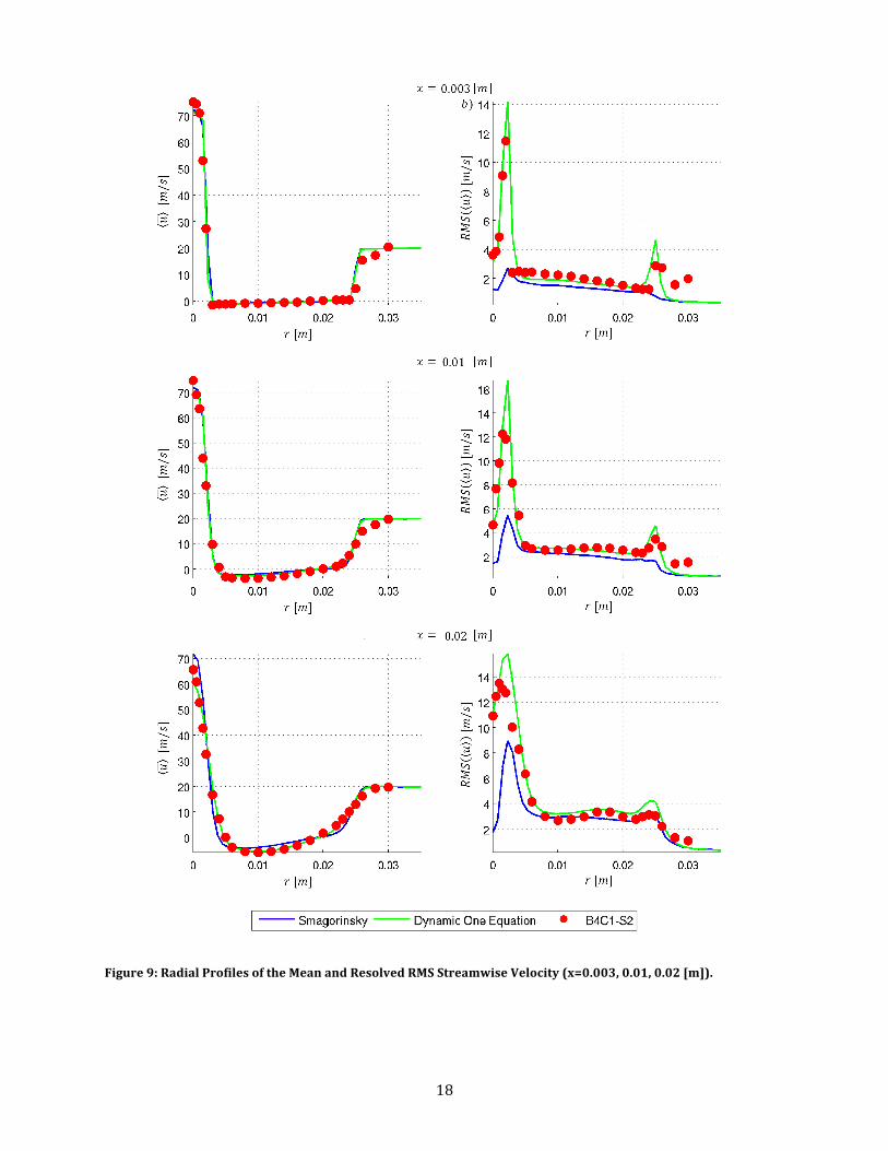
velocity profiles are accurate closer to the bluff, as shown in Figure 9. They however start to
diverge from the experimental values at Figure 10. Downstream, the overall agreement is
reasonable but near the centerline the Smagorinsky model over-‐predicts, and the Dynamic One
Equation model under-‐predicts the streamwise velocity. In both cases, the jet velocity is under-‐
predicted after the recirculation zone, or at approximately one bluff diameter (x = 0.50), as shown
in Figure 11. The streamwise velocity fluctuations are shown alongside the velocity profiles in
Figure 9 through Figure 11. Both models follow the experimental profile reasonably well, with
peaks in the profile consistent with the inner, central, and outer mixing layers. The Smagorinsky
model tends to under-‐predict the fluctuations close to the face of the bluff as shown in Figure 9, and
over-‐predict the fluctuations further from the bluff in Figure 10. The Dynamic One Equation model
shows closer agreement with the data across all sample points. The velocity profile in contours
greater than one bluff diameter tend to under-‐predict the free stream co-‐flow velocity of 20 m/s,
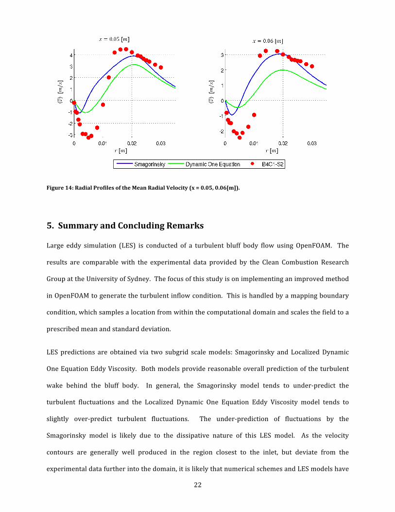
which is due to the over-‐prediction of the spread rate of the jet. The radial velocity profiles are
shown in Figure 12 through Figure 14. Both methods provide reasonable prediction of the radial
velocity at all locations.
Figure 4: Instantaneous Streamwise Filtered Velocity Iso-‐surfaces (clipped by X-‐Y plane)

15
Figure 5: Magnitude of Instantaneous Vorticity Iso-‐surfaces (clipped by X-‐Y plane)
Figure 6: Line Integral Convolution of Streamwise Filtered Velocity in Bluff Region, X-‐Y Plane
16
Figure 7: LES filtered Streamwise Velocity Contours Predicted by the Smagorinsky Model.
a) Smagorinsky, X-‐Y plane, Instantaneous contours of ⟨𝑢⟩
b) Smagorinsky, X-‐Z plane, Instantaneous contours of ⟨𝑢⟩
c) Smagorinsky, X-‐Y plane, Time-‐Averaged contours of ⟨𝑢⟩

17
Figure 8: LES filtered Streamwise Velocity Contours Predicted by the Dynamic One Equation Model.
a) Dynamic One Equation, X-‐Y plane, Instantaneous contours of ⟨𝑢⟩
b) Dynamic One Equation, X-‐Z plane, Instantaneous contours of ⟨𝑢⟩
c) Dynamic One Equation, X-‐Y plane, Time-‐Averaged contours of ⟨𝑢⟩
18
Figure 9: Radial Profiles of the Mean and Resolved RMS Streamwise Velocity (x=0.003, 0.01, 0.02 [m]).

19
Figure 10: Radial Profiles of the Mean and Resolved RMS Streamwise Velocity (x=0.03, 0.04, 0.05 [m]).

20
Figure 11: Radial Profiles of the Mean and Resolved RMS Streamwise Velocity (x=0.06 [m]).
Figure 12: Radial Profiles of the Mean Radial Velocity (x=0.003, 0.01 [m]).

21
Figure 13: Radial Profiles of the Mean Radial Velocity (x = 0.02, 0.03, 0.04[m]).
22
Figure 14: Radial Profiles of the Mean Radial Velocity (x = 0.05, 0.06[m]).
5. Summary and Concluding Remarks
Large eddy simulation (LES) is conducted of a turbulent bluff body flow using OpenFOAM. The
results are comparable with the experimental data provided by the Clean Combustion Research
Group at the University of Sydney. The focus of this study is on implementing an improved method
in OpenFOAM to generate the turbulent inflow condition. This is handled by a mapping boundary
condition, which samples a location from within the computational domain and scales the field to a
prescribed mean and standard deviation.
LES predictions are obtained via two subgrid scale models: Smagorinsky and Localized Dynamic
One Equation Eddy Viscosity. Both models provide reasonable overall prediction of the turbulent
wake behind the bluff body. In general, the Smagorinsky model tends to under-‐predict the
turbulent fluctuations and the Localized Dynamic One Equation Eddy Viscosity model tends to
slightly over-‐predict turbulent fluctuations. The under-‐prediction of fluctuations by the
Smagorinsky model is likely due to the dissipative nature of this LES model. As the velocity
contours are generally well produced in the region closest to the inlet, but deviate from the
experimental data further into the domain, it is likely that numerical schemes and LES models have

23
a significant role in the accuracy of these simulations. Altering the inlet parameters provides some
control over the velocity profiles; however, those profiles past the recirculation zone are always
under-‐predicted in the results. The predictions obtained from the Dynamic One Equation model
are more consistent with the experimental data, for both first and second order moments. This
work provides a preliminary implementation of a modified mapped boundary condition in
OpenFOAM by including additional controls to match a prescribed inflow condition. OpenFOAM
along with the new inlet boundary condition has shown to provide LES prediction of turbulent
flows past a bluff body with reasonable accuracy. The near field of the flow is favorably predicted.
The far field however shows less accuracy mainly near the centerline and due to over-‐prediction of
the spread rate of the jet. The modified mapping boundary condition has the potential for further
developments including additional control over second order statistics, and scaling to maintain a
specified distribution as well as parameters to control the behavior of the jet downstream.

24
References
[1] D. C. Wilcox, Turbulence modeling for CFD vol. 1. La Cañada, CA: DCW Industries, Inc., 1993.
[2] W. Rodi, "Comparison of LES and RANS calculations of the flow around bluff bodies," Journal of Wind Engineering and Industrial Aerodynamics, vol. 69–71, pp. 55-‐75, 1997.
[3] S. B. Pope, Turbulent Flows. New York, NY: Cambridge University Press, 2000.
[4] The University of Sydney. (2014). Bluff-‐Body Flows and Flames. Available: http://sydney.edu.au/engineering/aeromech/thermofluids/bluff.htm
[5] T. G. Drozda, "Implementation of LES/SFMDF for prediction of non-‐premixed turbulent flames," Ph.D. Dissertation, University of Pittsburgh, 2006.
[6] T. Drozda, M. Sheikhi, C. Madnia, and P. Givi, "Developments in formulation and application of the filtered density function," Flow, Turbulence and Combustion, vol. 78, pp. 35-‐67, 2007.
[7] D. A. Lysenko, I. S. Ertesvåg, and K. E. Rian, "Modeling of turbulent separated flows using OpenFOAM," Computers & Fluids, vol. 80, pp. 408-‐422, 2013.
[8] N. M. C. Salvador, M. T. Mendonça, and W. M. da Costa Dourado, "Large Eddy Simulation of bluff body stabilized flame with turbulent premixed flame," Guidelines of Workshop on Space Engineering and Technology, June 2012.
[9] G. Tabor, M. Baba-‐Ahmadi, E. de Villiers, and H. Weller, "Construction of inlet conditions for LES of turbulent channel flow," in Proceedings of the ECCOMAS congress, Jyväskylä, Finland, 2004.
[10] J. Volavy, M. Forman, and M. Jicha, "Influence of the turbulence representation at the inlet on the downstream flow pattern in LES of backward-‐facing step," EPJ Web of Conferences, vol. 25, 2012.
[11] OpenFOAM Foundation. (2014). OpenFOAM® Release History. Available: http://www.openfoam.org/download/history.php
[12] OpenFOAM Foundation. (2014). Parallel Computing. Available: http://openfoam.org/features/parallel-‐computing.php
[13] OpenFOAM Foundation. (2014). OpenFOAM® Programmer's C++ documentation -‐ Smagorinsky Class Reference. Available: http://foam.sourceforge.net/docs/cpp/a02317.html
[14] OpenFOAM Foundation. (2014). OpenFOAM® Programmer's C++ documentation -‐ dynOneEqEddy Class Reference. Available: http://foam.sourceforge.net/docs/cpp/a00580.html
[15] G. R. Tabor and M. H. Baba-‐Ahmadi, "Inlet conditions for large eddy simulation: A review," Computers & Fluids, vol. 39, pp. 553-‐567, 2010.


