
Large Eddy Simulation of a Stable Supersonic Jet
Impinging on a Flat Plate
A. Dauptain1, B. Cuenot2, and L.Y.M. Gicquel3
Cerfacs, 42 ave. G. Coriolis 31057 Toulouse - France
This paper describes a numerical study based on Large Eddy Simulation (LES) of
the flow induced by a supersonic jet impinging on a flat plate in a stable regime. This
flow involves very high velocities, shocks and intense shear layers. Performing LES
on such flows remains a challenge because of the shock discontinuities. Here, LES is
performed with an explicit third-order compressible solver using a unstructured mesh,
a centered scheme, and the Smagorinsky model. Three levels of mesh refinement (from
7 to 22 million cells) are compared in terms of instantaneous and averaged flow fields
(shock and recirculation zone positions), averaged flow velocity and pressure fields, wall
pressure, RMS pressure fields, and spectral content using one and two point analyses.
The effects of numerical dissipation and turbulent viscosity are compared on the three
grids and shown to be well controlled. The comparison of LES with experimental
data of Henderson et al. shows that the finest grid (a 22 M cell mesh) ensures grid-
independent results.
1 Post-Doctoral Searcher, CFD team, [email protected] Senior Searcher, CFD team, [email protected] Senior Searcher, CFD team, [email protected]
1
Nomenclature
c = sound speed, m/s
Cp = heat capacity at constant pressure, J.Kg−1.K−1
d = nozzle inner diameter, 2.54 cm
h = wall-nozzle distance, 10.5664 cm
p = pressure, Pa
r = cylindrical coordinate : distance from the axis, m
R = ideal gas constant, 8.314 J.K−1.mol−1
t = time, s
T = temperature, K
u, v, w = velocity components, m/s
W = molar mass of air, 28.85 g.mol−1
~x, x, y, z = cartesian coordinates: vector and components, m
∆x = typical cell size, m
∆t = computational time step, s
∆Cell = size of compression-expansion zone, m
Φ = phase shift, rad
µ = dynamic viscosity, Kg.m−1.s−1
ρ = density, Kg/m3
¯ = spatial filtering of large eddy simulation
˜ = Favre averaging
ˆ = Fourier transform
<>mean = mean, in the process of time-averaging
<>rms = root mean square or quadratic mean, in the process of time-averaging
<>az. = azimuthal averaging
2
I. Introduction
In recent years, Large Eddy Simulations (LES) have demonstrated their ability to predict the
behavior of weakly compressible turbulent flows [1–5]. LES applications to supersonic flows however
remain to be validated. Typical examples of non-reacting supersonic flows with strong industrial
interests are impinging jets which appear in leaks of high pressure tanks and pipes or breaches in
the outer structure of reentry vehicles [6]. Such jets can exhibit tone-producing modes that depend
on the jet exit distance to the wall and nozzle pressure ratio [7–9]. They have been studied for as-
tronautics (multi-stage rocket separation, attitude control thruster), aeronautics (jet-engine exhaust
impingment. vertical take-off stability) or turbomachinery (gas turbine blade thermal failure). The
work of Donaldson and Snedeker in 1971 [10, 11] describes the physics of circular jets impinging
on spherical, normal and oblique surface. A later work from Lamont and Hunt [12] focuses on the
near field jet impingement zone, showing the link between the overall load on the plate and the
momentum flux at the nozzle lip. A fair amount of studies focused in the eighties and nineties on
the unsteadiness of such flows, e.g. Ho and Nosseir [13], Kuo and Dowling [14] .
Computational approaches based on the method of characteristics or Euler solvers are com-
mon tools for supersonic jets. Reynolds Averaged Navier-Stokes (RANS) simulations address the
viscous features and the effect of turbulence. These numerical models are widely developed and
computationally efficient but they are limited to stationnary flows. Unsteady phenomena linked
to turbulence are best addressed with LES, which provides time-dependent filtered quantities of
one flow realization. LES has been used with success to reproduce the intermittent and unsteady
tone-producing modes of free jets [15] and cavities [16]. Combined with advanced diagnostics to
take advantage of the spatial and temporal description of the problem, LES can provide specific
informations about non-linear interactions or causality of phenomena.
From a chronological point of view, specific numerical techniques have been developed for su-
personic jets since the fifties. The work of Ferri at NACA [17] illustrates the sophistication of the
characteristics approach in the context of transonic aircrafts. The BAMIRAC report of Adamson [18]
reviews several approximate methods to calculate the main inviscid features of highly underexpanded
jets. Between 1990 and 2000, various Euler or RANS solvers took advantage of adaptive gridding
3
or multigrid [19–23]. Oscillating impinging jets were simulated by Kuo [14] and Sakakibara [24].
Improvements of turbulence models lead to accurate quantitative predictions [25], and unsteady
RANS succeded in reproducing screech phenomenon [26], in spite of a narrow bandwith description
around the discrete tone. In 2003, Arunajatesan [27] used LES for steady supersonic impingement
of jets, to predict the major quantities of the flow such as the averaged pressure loads and cen-
terline velocity. A few studies focused also on planar [28] and rectangular [29] supersonic screech
jets. Note that direct computation of noise by LES has been also demonstrated in subsonic config-
urations [30–32]. More recently, hybrid methods mixing RANS and LES approaches were applied
successfully to compressible mixing layers [33] and to supersonic jets [34], to address the problem
of wall generated-turbulence, a reccurent LES bottleneck [35]. Note that wall-generated turbulence
in the nozzle of a free jet does have a clear impact on the noise generated and special care must be
taken (e.g. [15]) for stable regimes, but it is not first-order in the loud discrete tones of unstable
impinging jets.
Table 1 presents a selection of numerical works in the last decade related to similar configura-
tions. The degrees of freedom are the total number of unknowns. WENO approaches having a high
CPU cost, the simulation domain and related grids are significantly smaller. Structured grids are
mainly used since the academic impingement configuration is geometrically simple. On the other
hand, unstructured grids are attractive for the short human time spent in the gridding phase, the
freedom of refinement/coarsening in any direction, and its ability to deal with complex geometries.
The present work describes a LES of a supersonic jet impinging on a wall using a centered
scheme with hyperviscosity at shocks and unstructured grids. The paper is organized as follows.
The experimental target configuration is introducedi in section II, with a brief flow description.
Then, the numerical method is presented and commented with particular stress on shock-capturing
technique and high performance computing (section III). The analysis is focused on the validation of
time-averaged quantities with respect to experimental data, the observation of several flow features
referenced in the litterature, and the energy distribution through spectral analysis. A specific
attention is devoted to the influence of the mesh on the LES solution. This study concludes with a
discussion on the pros and cons of LES applied to such flows.
4

Table 1 Selection of previous numerical works
Case Name Year Method Mesh Volume Size ( d.o.f.)
Imp. jet Arunajatesan [27] 2002 LES Struct. 30o sector 5 × 2.78 106
Mix. lay. Georgiadis [36] 2003 Hybrid Struct. 3D slab. 5 × 0.87 106
Free jet Cheng [37] 2005 ILES-WENO Struct. 2D Axisym. 4 × 87.5 103
Screech. Jet Berland [15] 2006 LES Struct. 3D slab 5 × 16.3 106
Ctrld. Jet∗ Chauvet [38, 39] 2007 RANS & Hybrid Struct. 3D 5 × 10.5 106
Screech. Jet Singh [40] 2007 LES-WENO Struct. 2D Axisym. 4 × 210 103
Launcher Nozzle Deck [41] 2009 Hybrid Struct. 3D 5 × 11 106
Imp. Jet Present work - LES Unstruct. 3D 5 × 3.8 106
∗
Complex geometry with mixing enhancement by control jets.
II. Target Configuration
Standing at the intersection of screech investigation and impinging jets, the experimental work of
Henderson [7] is of particular interest to LES. Indeed, the variation of a single geometric parameter,
namely the nozzle to plate distance, leads either to silent or tone-producing flows. The current work
aims at assessing the validity of LES on one of the stable cases.
A. Flow Description and Parameterization
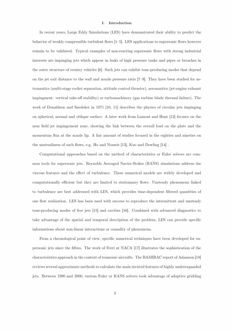
The flow parameters governing the response of free supersonic jets are: the convergent nozzle
of diameter d and the Nozzle total Pressure to ambient static pressure Ratio (NPR). For a NPR
approaching 4, shock structures take place at the rim of the nozzle. The fluid goes through a Prandtl-
Meyer expansion to recover the ambient pressure value. Mach reflections converge to generate a
cone-shaped weak shock ended by a disc-shaped strong shock, Fig. 1a. The weak and strong shocks
merge into a triple point giving birth to a reflected oblique shock and a shear line. For free jets,
this inviscid pattern composed of the weak, strong, reflected shocks and shear lines is repeated
several times downstream. The size of this expansion-compression cell ∆cell was measured for a
wide range of configuration [42]. The succession of cells is the primary mechanism by which the jet
inner pressure adapts to reach the ambient state.
5
For impinging configurations, a large obstacle (usually a wall, Fig. 1b) is blocking the supersonic
free jet plume. The most critical configuration appears if the distance h from the jet nozzle to the
wall is shorter than the inviscid core. For that case, the strong pressure drop issued by the strong
shock creates a near wall flow recirculation bubble with a contact line separating the main jet and
the recirculated flow as shown on Fig. 1b. The main effect of this impact of the jet on the wall is
the generation of strong acoustic waves and depending on the NPR, the wall distance h/d or the
plate dimension, discrete acoustic tones may be produced.
Weak shock Weak shockStrong shock Strong shockReflected shock Reflected shockShear line Shear line
Contact line
Recirculation zoneMixing layer Mixing layer
Acoustic wave
h
dd
a) Free Jet b) Impinging jet
∆cell ∆cell ∆cell
~x
~y
~z
~r
Fig. 1 Impacting jet on a flat plate: flow description and main geometrical parameters.
Although the extreme case of the tone dominated impacting jet is of clear interest, a simpler
stable case is retained for this study for the LES validation. For this reason the present work focuses
on the stable case studied experimentally by Henderson et al. [7] and defined by NPR = 4.03,
h/d = 4.16.
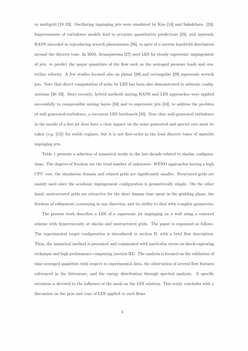
B. Experimental Apparatus and Diagnostics
The experiment performed by Henderson et al. [7] uses the Small Hot Jet Aeroacoustic rig (SH-
JAR), a facility of the AeroAcoustic Propulsion Laboratory (AAPL) at the NASA Glenn Research
Center, Fig. 2a. In this specific experiment, the convergent nozzle has a one inch exit diameter d,
6
a) b)0 0
1
1
2
2
3
3 4 5
1.65 2.08 2.66 2.80 3.65 4.16 4.66
Zone of silence
Tones observed
Present simulations
h/d
λ/d
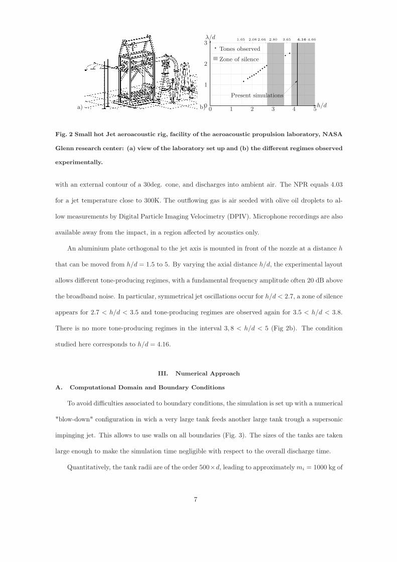
Fig. 2 Small hot Jet aeroacoustic rig, facility of the aeroacoustic propulsion laboratory, NASA
Glenn research center: (a) view of the laboratory set up and (b) the different regimes observed
experimentally.
with an external contour of a 30deg. cone, and discharges into ambient air. The NPR equals 4.03
for a jet temperature close to 300K. The outflowing gas is air seeded with olive oil droplets to al-
low measurements by Digital Particle Imaging Velocimetry (DPIV). Microphone recordings are also
available away from the impact, in a region affected by acoustics only.
An aluminium plate orthogonal to the jet axis is mounted in front of the nozzle at a distance h
that can be moved from h/d = 1.5 to 5. By varying the axial distance h/d, the experimental layout
allows different tone-producing regimes, with a fundamental frequency amplitude often 20 dB above
the broadband noise. In particular, symmetrical jet oscillations occur for h/d < 2.7, a zone of silence
appears for 2.7 < h/d < 3.5 and tone-producing regimes are observed again for 3.5 < h/d < 3.8.
There is no more tone-producing regimes in the interval 3, 8 < h/d < 5 (Fig 2b). The condition
studied here corresponds to h/d = 4.16.
III. Numerical Approach
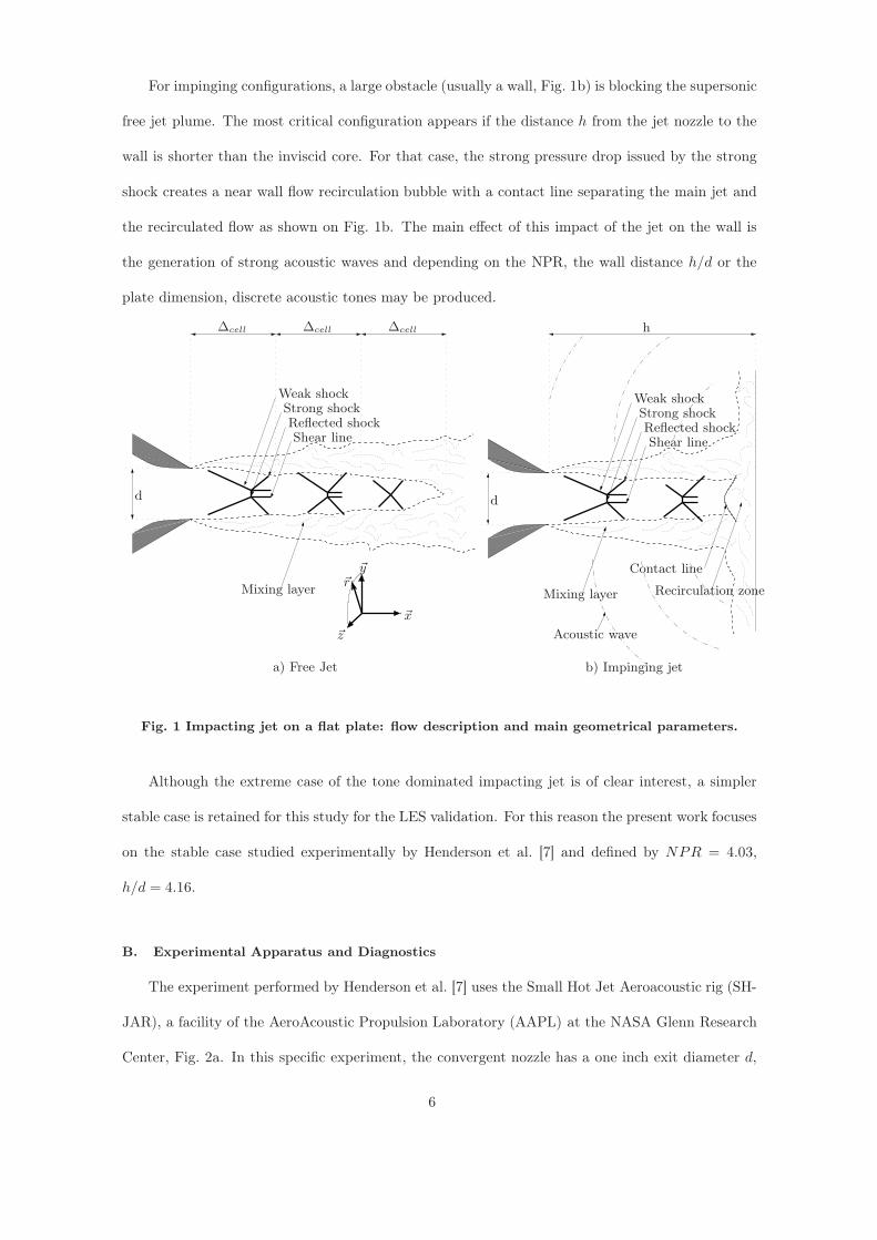
A. Computational Domain and Boundary Conditions
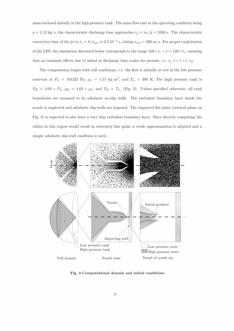
To avoid difficulties associated to boundary conditions, the simulation is set up with a numerical
"blow-down" configuration in wich a very large tank feeds another large tank trough a supersonic
impinging jet. This allows to use walls on all boundaries (Fig. 3). The sizes of the tanks are taken
large enough to make the simulation time negligible with respect to the overall discharge time.
Quantitatively, the tank radii are of the order 500×d, leading to approximately mi = 1000 kg of
7
mass enclosed initially in the high pressure tank. The mass flow rate at the operating condition being
q = 1.12 kg/s, the characteristic discharge time approaches td = mi/q = 1000 s. The characteristic
convective time of the jet is tc = h/ujet ≈ 2.5 10−4 s, taking ujet = 300 m/s. For proper exploitation
of the LES, the simulation discussed below corresponds to the range 100×tc < t < 120×tc, ensuring
that no transient effects due to initial or discharge time scales are present: i.e. tc << t << td.
The computation begins with still conditions, i.e. the flow is initially at rest in the low pressure
reservoir at PL = 101325 Pa, ρL = 1.15 kg/m3, and TL = 300 K. The high pressure tank is
PH = 4.03 × PL, ρH = 4.03 × ρL, and TH = TL, (Fig. 3). Unless specified otherwise, all tank
boundaries are assumed to be adiabatic no-slip walls. The turbulent boundary layer inside the
nozzle is neglected and adiabatic slip-walls are imposed. The impacted flat plate (vertical plane on
Fig. 3) is expected to also have a very thin turbulent boundary layer. Since directly computing the
eddies in this region would result in extremely fine grids, a crude approximation is adopted and a
simple adiabatic slip-wall condition is used.
���������������������������������������������������������������������������������������������������������������������������������
���������������������������������������������������������������������������������������������������������������������������������
����������������������������������������������������������������������������������������������������������������������������������������������������������������������������������������������������������������������������������������������������������������������������������������������������������������������������������������������������������������
����������������������������������������������������������������������������������������������������������������������������������������������������������������������������������������������������������������������������������������������������������������������������������������������������������������������������������������������������������������������������������������������������������������������������������������������������������������������������������������������������������������������������������������������������������������������������������������������������������������������������������������������������������������������������������������������������������������
������������������������������������������������������������������������������������������������������������������������������������������������������������������������������������������������������������������������������������������������������������������������������������������������������������������������������������������������
����������������������������������������������������������������������������������������������������������������������������������������������������������������������������
����������������������������������������������������������������������������������������������������������������������������������������������������������������������������
������������������������������������������������������������������������
������������������������������������������������������������������������
��������������������������������������������������������������������������������
��������������������������������������������������������������������������������
������������������������
������������������������
��������������������������������
��������������������������������
Mes
h
Full domain Nozzle zone Detail of nozzle tip
Nozzle
Impacting wall
High pressure tankLow pressure tank
High pressure state
Low pressure state
Initial gradient
Fig. 3 Computational domain and initial conditions
8
The grid convergence analysis uses three unstructured tetrahedra grids, generated for the same
geometry (Table. 2). The leading parameter is the number of nodes in the diameter of the injector.
As the solver is explicit, the time step ∆t is limited by the smallest cell size ∆x and the fastest
acoustic propagation speed u + c, with u standing for velocity and c for sound speed (Courant-
Friedrichs-Lewy criterion [43]):
∆t < CFLmin(∆x)
max(u + c)(1)
The explicit scheme is third-order in time and space and yields stable numerical solutions provided
that CFL ≤ 0.7 [44].
The grid generation package Centaur (http://www.centaursoft.com) is used to generate the
three meshes. Throughout the following document, x, y, and z are respectively used for the axial,
transverse, and spanwise components of the position vector ~x, while r is used for the radial distance
from the jet symmetry axis. Mesh refinement allows a maximum streching ratio of 1.7 between
tetrahedrons and 1.5 beween edges. Cell size distribution is depicted in Fig. 4. A uniform grid size
is enforced in the region of interest. The jet impact zone is also uniformly discretized for a region
defined by r/d ≤ 2. Finally, a buffer zone imposes linear coarsening for the three meshes away
from the impact. All grid characteristics are detailed in Table 2 with their computational costs in
Table 3. In this last table, Subscripts cpu (resp. hum.) denotes time used by one processor (resp.
human time).
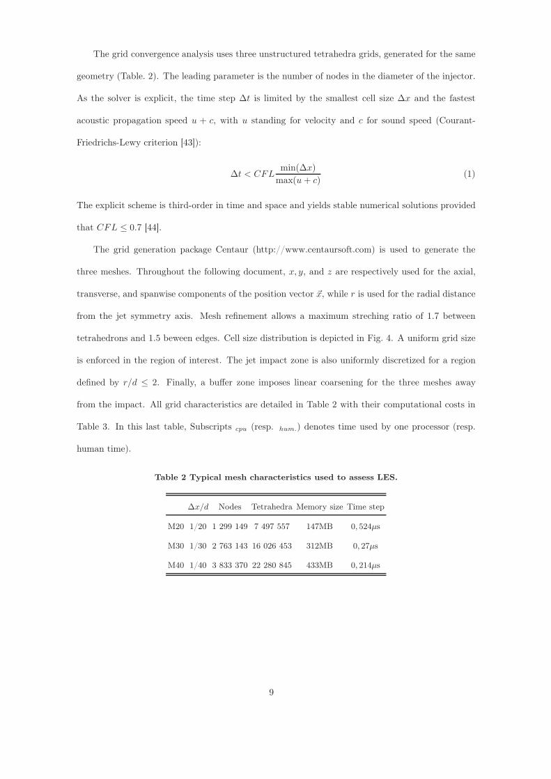
Table 2 Typical mesh characteristics used to assess LES.
∆x/d Nodes Tetrahedra Memory size Time step
M20 1/20 1 299 149 7 497 557 147MB 0, 524µs
M30 1/30 2 763 143 16 026 453 312MB 0, 27µs
M40 1/40 3 833 370 22 280 845 433MB 0, 214µs
9
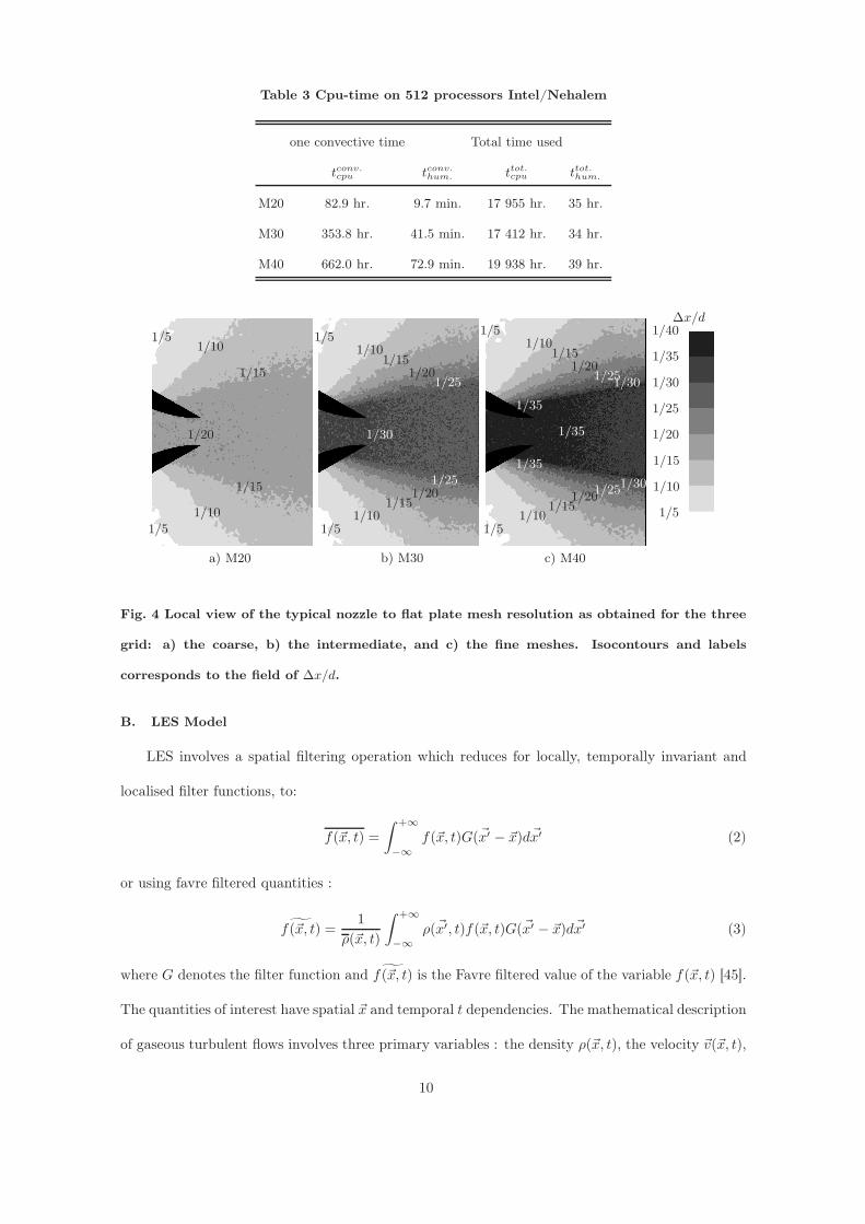
Table 3 Cpu-time on 512 processors Intel/Nehalem
one convective time Total time used
tconv.cpu tconv.
hum. ttot.cpu ttot.
hum.
M20 82.9 hr. 9.7 min. 17 955 hr. 35 hr.
M30 353.8 hr. 41.5 min. 17 412 hr. 34 hr.
M40 662.0 hr. 72.9 min. 19 938 hr. 39 hr.
a) M20 b) M30 c) M40
1/5
1/10
1/15
1/20
1/25
1/30
1/35
1/401/5
1/5
1/5 1/5
1/51/5
1/10
1/10
1/101/10
1/101/10 1/15
1/151/151/15
1/151/15
1/201/20
1/20
1/201/20
1/25
1/25
1/25
1/25 1/30
1/30
1/30 1/35
1/35
1/35
∆x/d
Fig. 4 Local view of the typical nozzle to flat plate mesh resolution as obtained for the three
grid: a) the coarse, b) the intermediate, and c) the fine meshes. Isocontours and labels
corresponds to the field of ∆x/d.
B. LES Model
LES involves a spatial filtering operation which reduces for locally, temporally invariant and
localised filter functions, to:
f(~x, t) =
∫ +∞
−∞
f(~x, t)G(~x′ − ~x)d~x′ (2)
or using favre filtered quantities :
˜f(~x, t) =1
ρ(~x, t)
∫ +∞
−∞
ρ(~x′, t)f(~x, t)G(~x′ − ~x)d~x′ (3)
where G denotes the filter function and ˜f(~x, t) is the Favre filtered value of the variable f(~x, t) [45].
The quantities of interest have spatial ~x and temporal t dependencies. The mathematical description
of gaseous turbulent flows involves three primary variables : the density ρ(~x, t), the velocity ~v(~x, t),
10
and the total energy E(~x, t) ≡ es + 1/2~v · ~v where es is the sensible energy.
The fluid follows the ideal gas law : p = ρTR/Wair and es =∫ T
0CpdT − p/ρ, where T is the
temperature, Cp the fluid heat capacity at constant pressure. The viscous stress tensor and the heat
diffusion use classical gradient approaches. The fluid viscosity follows Sutherland’s law and the heat
diffusion follows Fourier’s law.
Filtering the instantaneous set of transport equations yields the LES equations, which need
closure models [46, 47]. The Sub-Grid-Scale (SGS) turbulent velocity tensor is modelled using
the turbulent viscosity model of Smagorinsky and the Boussinesq assumption [48–50]. The eddy
diffusivity is also used along with a turbulent Prandtl number. Note that the performance of the
models might be improved through the use of a dynamic formulation [50–54] or more advanced type
of closures [55–57] which were not tested here.
C. Shock-capturing Scheme and Artificial Viscosity
The shock pattern present in supersonic jets is one of the main difficulties in LES of high speed
flows [58]. LES solvers able to handle shocks rely on either localized artificial viscosity [59–62], or on
spatial schemes adapted to handle discontinuities while preserving the positiveness of the solution,
giving birth to a wide family of techniques ranging from the initial approximated Riemann solvers
(FCT TVD) to the WENO (Weighted Essentially No Oscillatory Schemes [63]). WENO schemes
are attractive for LES because of their very high precision [40] but imply longer computational
time. In the present work, centered schemes were chosen because of their superior performance (low
dissipation) in shock free regions. To preserve the positivity of the solution in regions where strong
gradients exist, a hyperviscosity β is introduced in the viscous stress tensor τij , using the approach
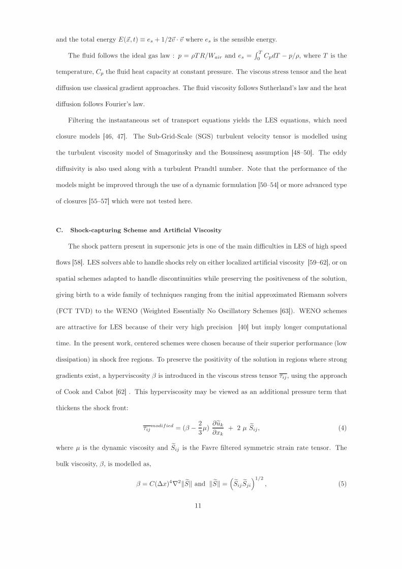
of Cook and Cabot [62] . This hyperviscosity may be viewed as an additional pressure term that
thickens the shock front:
τijmodified = (β − 2
3µ)
∂uk
∂xk+ 2 µ Sij , (4)
where µ is the dynamic viscosity and Sij is the Favre filtered symmetric strain rate tensor. The
bulk viscosity, β, is modelled as,
β = C(∆x)4∇2‖S‖ and ‖S‖ =(Sij Sji
)1/2
, (5)
11
where C is fixed to 5 [64]. This viscosity acts on the very sharp velocity gradients characterizing
shocks but goes back to zero in zones where the velocity evolves smoothly [65].
IV. Results and Discussion
The simulation of this stable case is validated by comparing time-averaged and instantaneous
LES fields with experimental results. Impact of the mesh resolution impact on the LES results is
studied afterwards. This last part includes the observation of instantaneous flow quanties, time-
averaged values, and energy distribution through spectral analysis.
A. Mean Flow Topology and Features
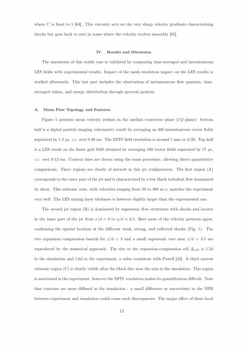
Figure 5 presents mean velocity isolines in the median transverse plane (~x ~y plane): bottom
half is a digital particle imaging velocimetry result by averaging on 400 instantaneous vector fields
separated by 1.2 µs, i.e. over 0.48 ms. The DPIV field resolution is around 1 mm or d/20. Top half
is a LES result on the finest grid M40 obtained by averaging 160 vector fields separated by 57 µs,
i.e. over 9.12 ms. Contour lines are drawn using the same procedure, allowing direct quantitative
comparisons. Three regions are clearly of interest in this jet configuration. The first region (A)
corresponds to the outer part of the jet and is characterized by a low Mach turbulent flow dominated
by shear. This subsonic zone, with velocities ranging from 50 to 300 m/s, matches the experiment
very well. The LES mixing layer thickness is however slightly larger than the experimental one.
The second jet region (B) is dominated by supersonic flow structures with shocks and locates
in the inner part of the jet from x/d = 0 to x/d ≈ 3.5. Here most of the velocity patterns agree,
confirming the spatial location of the different weak, strong, and reflected shocks (Fig. 1). The
two expansion/compression barrels for x/d < 3 and a small supersonic tore near x/d = 3.5 are
reproduced by the numerical approach. The size or the expansion-compression cell ∆cell is 1.5d
in the simulation and 1.6d in the experiment, a value consistent with Powell [42]. A third narrow
subsonic region (C) is clearly visible after the Mach disc near the axis in the simulation. This region
is mentioned in the experiment: however the DPIV resolution makes its quantification difficult. Note
that contours are more diffused in the simulation : a small difference or uncertainty in the NPR
between experiment and simulation could cause such discrepancies. The major effect of these local
12
differences in the inner supersonic and outer subsonic regions is that the overall jet opening angle
differs slightly in LES and in the experiment. The fourth zone of interest (D) is the recirculation
bubble which forms along the central axis of the jet in the vicinity of the plate. This subsonic region
is characterized by an abrupt deceleration and takes on the shape of a cone whose base is located
on the vertical wall: it is very well predicted by LES.
A
B
C
D
Simulation
Experiment
y/d
x/d
0
0
−1
1
1
2 3 4
100
100
200
300
300
400
400
400400
400
400 400
400
500
50
50
50
50
150
150
250
350350350
350350
450
450
450
450
Fig. 5 Comparison of time averaged velocity fields as obtained by the fine mesh simulation
(top half) and experiment (bottom half). Contour values in m/s.
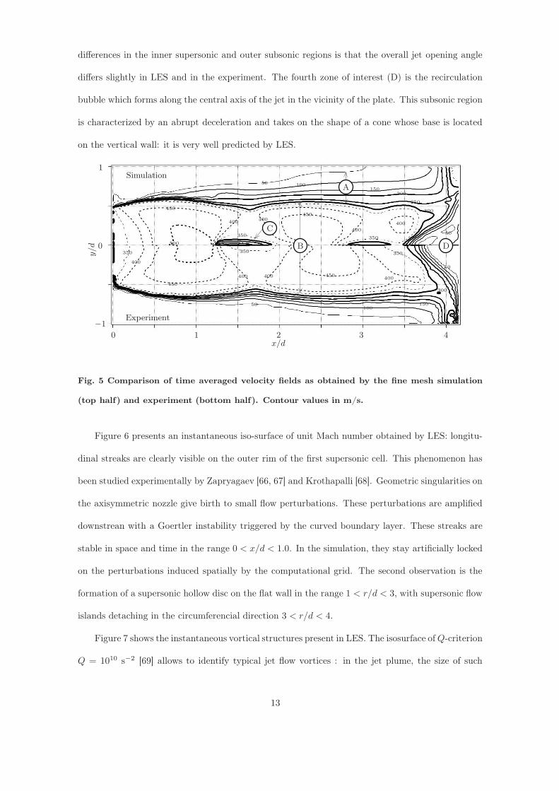
Figure 6 presents an instantaneous iso-surface of unit Mach number obtained by LES: longitu-
dinal streaks are clearly visible on the outer rim of the first supersonic cell. This phenomenon has
been studied experimentally by Zapryagaev [66, 67] and Krothapalli [68]. Geometric singularities on
the axisymmetric nozzle give birth to small flow perturbations. These perturbations are amplified
downstrean with a Goertler instability triggered by the curved boundary layer. These streaks are
stable in space and time in the range 0 < x/d < 1.0. In the simulation, they stay artificially locked
on the perturbations induced spatially by the computational grid. The second observation is the
formation of a supersonic hollow disc on the flat wall in the range 1 < r/d < 3, with supersonic flow
islands detaching in the circumferencial direction 3 < r/d < 4.
Figure 7 shows the instantaneous vortical structures present in LES. The isosurface of Q-criterion
Q = 1010 s−2 [69] allows to identify typical jet flow vortices : in the jet plume, the size of such
13
vortices is approximately d/5 (about four computational cells) while on the plate, they reach d/10
(about sixteen computational cells). In the mixing layer, the structures are oblique between the
longitudinal axis and the azimuthal direction. Vortices on the wall are aligned azimuthally because
of the radial stretching generated by the jet impact on the plate and the flow orientation in this
region.
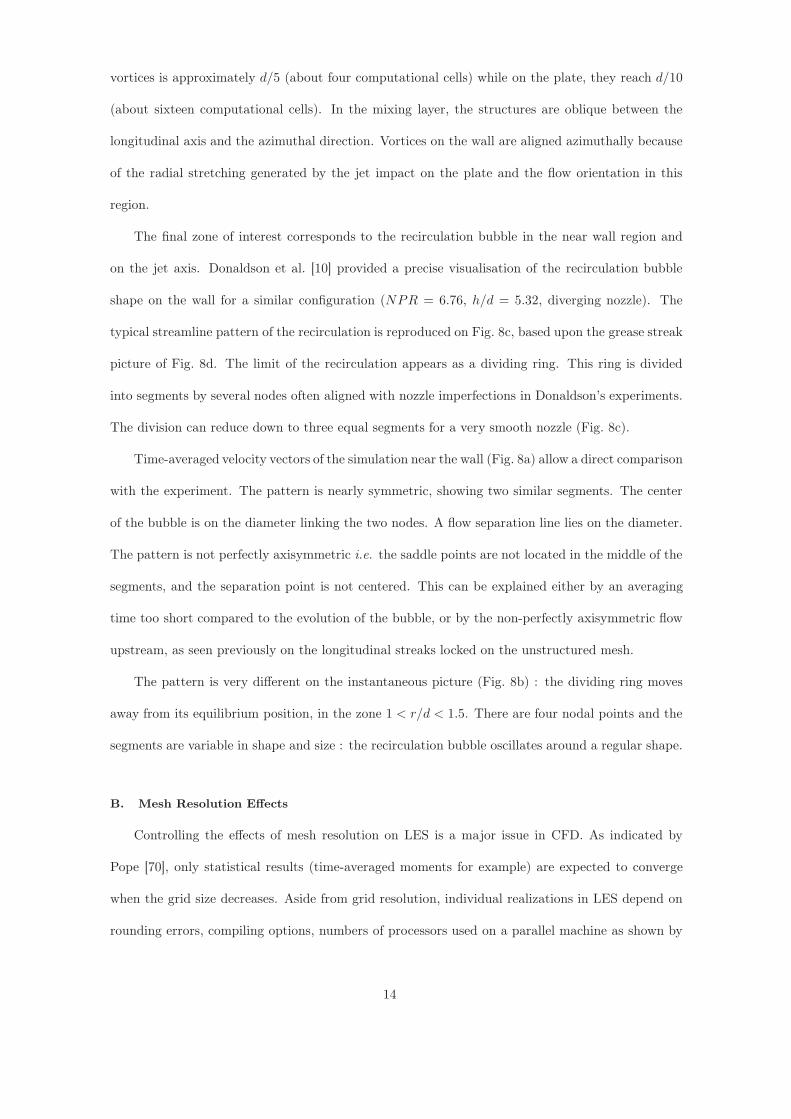
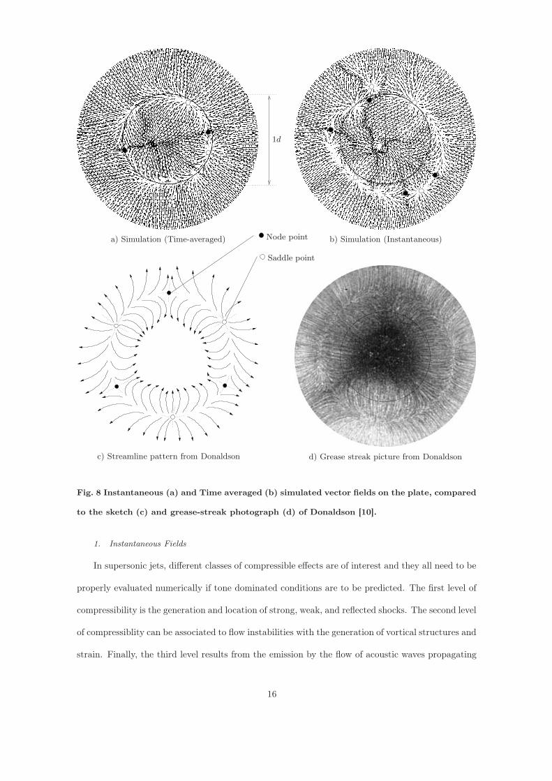
The final zone of interest corresponds to the recirculation bubble in the near wall region and
on the jet axis. Donaldson et al. [10] provided a precise visualisation of the recirculation bubble
shape on the wall for a similar configuration (NPR = 6.76, h/d = 5.32, diverging nozzle). The
typical streamline pattern of the recirculation is reproduced on Fig. 8c, based upon the grease streak
picture of Fig. 8d. The limit of the recirculation appears as a dividing ring. This ring is divided
into segments by several nodes often aligned with nozzle imperfections in Donaldson’s experiments.
The division can reduce down to three equal segments for a very smooth nozzle (Fig. 8c).
Time-averaged velocity vectors of the simulation near the wall (Fig. 8a) allow a direct comparison
with the experiment. The pattern is nearly symmetric, showing two similar segments. The center
of the bubble is on the diameter linking the two nodes. A flow separation line lies on the diameter.
The pattern is not perfectly axisymmetric i.e. the saddle points are not located in the middle of the
segments, and the separation point is not centered. This can be explained either by an averaging
time too short compared to the evolution of the bubble, or by the non-perfectly axisymmetric flow
upstream, as seen previously on the longitudinal streaks locked on the unstructured mesh.
The pattern is very different on the instantaneous picture (Fig. 8b) : the dividing ring moves
away from its equilibrium position, in the zone 1 < r/d < 1.5. There are four nodal points and the
segments are variable in shape and size : the recirculation bubble oscillates around a regular shape.
B. Mesh Resolution Effects
Controlling the effects of mesh resolution on LES is a major issue in CFD. As indicated by
Pope [70], only statistical results (time-averaged moments for example) are expected to converge
when the grid size decreases. Aside from grid resolution, individual realizations in LES depend on
rounding errors, compiling options, numbers of processors used on a parallel machine as shown by
14

4d
3d
Supersonic layer
Gœrtler vortices
Fig. 6 Instantaneous isosurface of unit Mach number as obtained by LES.
4d
3d2d
1d
Azimuthal vortices
Mixing layer
Fig. 7 Instantaneous view of the Q criterium isosurface Q = 11010 s−2 obtained by LES.
Senoner et al. [71, 72]. Therefore verifying grid effects in LES is a difficult exercice. In the present
case, the influence of mesh is tested by repeating the same simulations on three grids containing
7.5, 16, and 22 M cells. For all grids, time-averaged velocity and pressure fields are compared
(Section IVB 2). Power spectral densities are also studied in Section IVB 3.
15
a) Simulation (Time-averaged) b) Simulation (Instantaneous)
c) Streamline pattern from Donaldson d) Grease streak picture from Donaldson
1d
Node point
Saddle point
Fig. 8 Instantaneous (a) and Time averaged (b) simulated vector fields on the plate, compared
to the sketch (c) and grease-streak photograph (d) of Donaldson [10].
1. Instantaneous Fields
In supersonic jets, different classes of compressible effects are of interest and they all need to be
properly evaluated numerically if tone dominated conditions are to be predicted. The first level of
compressibility is the generation and location of strong, weak, and reflected shocks. The second level
of compressiblity can be associated to flow instabilities with the generation of vortical structures and
strain. Finally, the third level results from the emission by the flow of acoustic waves propagating
16
in the medium. These effects can be distinguished by the density gradient ‖∇ρ‖ which they induce:
strong for shocks, medium for vortices and small for acoustics. Three different black and white
scales with different orders of magnitude are shown in Fig. 9 for instantaneous LES fields obtained
on the three different meshes.
Based on this diagnostic, simulations M30 and M40 (i.e. intermediate and fine grid resolutions
respectively) appear very similar while simulation M20 (i.e. coarse grid) deviates significantly from
the two others due to excessive dissipation; in particular the corrugated shear layer (Fig. 12I) and
the acoustic waves (Fig. 12III) are excessively smeared on M20 (Fig. 12a).
An illustration of the instantaneous Mach number distribution for the three grid resolutions
at the same instant is given in Fig. 10. The coarse grid LES M20 clearly attenuates most of the
dynamics. It is able to place properly the different inner jet supersonic structures but produces
highly damped unsteady motions in the outer jet mixing layers and along the plate. An increase
of resolution improves the local sharpness of the different structures as observed on M30. The fine
grid resolution M40 reveals more intermittency in the Mach distribution especially along the plate
as well as sharper supersonic patterns in the inner jet region.
As expected with LES, as the local grid resolution increases, more flow structures are explicitely
resolved and the resolved flow energy content is increased. It must be compared to dissipation
effects due to artificial viscosity, shock-capturing, and flow laminar or turbulent viscosities. These
questions are investigated below using instantaneous views of various ratios of viscosities for three
grid resolutions.
The artificial viscosity (µA.V.) resulting from the shock-capturing scheme and the necessary
numerical stabilization is given in Fig. 11. For all meshes, artificial damping is low and localized
along shear layers and shock lines. Compared to the laminar contribution the ratio remains low: it
exceeds unity on M40 only in zones of shocks, something which can not be avoided. Simulations
M30 and M40 exhibit similar results, with artificial viscosity lower than the laminar one in some
parts of the jet (Fig 11b and 11c): in the range 1−10 on the shear layer and around 10 on the shock
lines. Note nonetheless that LES with M20 yields significantly more damped supersonic structures,
in agreement with an artificial to laminar viscosity ratio which saturates around 10 in the core of the
17

∇ρ[Kg/m4]
∇ρ[Kg/m4]
∇ρ[Kg/m4]
a) M20 b) M30 c) M40
1000
100
10
0
0
0
I)
II)
III)
Fig. 9 Magnitude of the density gradient for three ranges of scale and for the same instanta-
neous field obtained on the three meshes at the same instant: Top I: large values, supersonic
patterns; Middle II: intermediate values, shear layers; Bottom III: small values, acoustic
waves. The diagnostic is provided for the ~x~y plane going through the central axis of the jet.
jet (Fig. 11a). Nozzle lip, mach disc and top of recirculation bubble are the most damped regions
with a ratio close to 30 for all meshes. From a numerical point of view, Fig. 11 confirms the correct
behaviour of the strategy devised to handle such flows with LES. As the mesh resolution increases,
the zones where artificial viscosity is added reduce in intensity and become highly localized.
The turbulent viscosity (µTurb.) to laminar viscosity ratio is provided on Fig. 12 and is to be
compared to Fig. 11 for the same grids: µTurb. is created by the subgrid scale turbulent model in
18

Mach
a) M20 b) M30 c) M40
2.6
2.0
1.5
1.0
0.5
0.0
Fig. 10 Instantaneous Mach number field as obtained on the three meshes. The diagnostic is
provided for the xy plane going through the central axis of the jet.
µA.V.
µLam.
a) M20 b) M30 c) M40
100
10
1
0.1
0.01
Fig. 11 Field of ratio of artificial Viscosity to Laminar Viscosity. White contours are drawn
for ratios equal to unity (thin line) and 30 (bold line).
regions of high shear and strain, meeting the requirement of LES. Its intensity reaches values ranging
from 10 to 40 times the laminar viscosity in the turbulent zones and is roughly 10 times superior to
the artificial viscosity levels of Fig 11. Simulations M30 and M40 yield a ratio µTurb./µLam. close
to 10 in the shear layer of the jet (Fig. 12b and 12c) while simulation M20 shows higher levels of
turbulent viscosity (closer to 100) over the entire shear layer (Fig 12a).
To summarize, Mach number and density gradient fields are similar for meshes M30 and M40.
Artificial and turbulent viscosity levels are reasonable and localized in shock and shear regions.
19

µT urb.
µLam.
a) M20 b) M30 c) M40
1000
100
10
1
0.1
Fig. 12 Field of ratio of Turbulent Viscosity to Laminar Viscosity. White contour are drawn
for ratios equal to 10 (thin line) and 100 (bold line).
2. Mean Quantities
Time-averaged values are obtained in the range 80 < t/tc < 100 with a sampling close to
0.1 × tc and compared for the three meshes M20, M30, and M40. For notation, < u >mean (resp.
< p >mean) is the time-averaged value of the velocity u (resp. pressure p). < u >rms denotes
root mean square velocity of the resolved field, without de-filtering technique or subgrid model
inclusion [46].
The longitudinal profiles of pressure and velocity are displayed on Fig. 13. The velocity fields
estimated from Digital Particles Imaging Velocimetry (DPIV) in Henderson’s experiment [7] are
compared to the three simulations in Fig. 13a. The two high velocity zones for x/d = 1 and
x/d = 2.5 are well reproduced. Simulations M30 and M40 both show a strong deceleration after
these high speed zones, while simulation M20 is apparently closer to experimental observations.
This gap can be explained both by the underestimation of the turbulence behind the Mach disc
in the simulation and bias of DPIV in strong deceleration and sharp gradients. For example, the
subsonic bubble visible in Fig. 5 has a diameter of 0.1d = 2.54 mm while the spatial resolution of
the DPIV is 1 mm: the same profile taken 1 mm away from the axis would not show the axial
subsonic zone. Time-averaged pressure is decreasing in the recirculation zone : a better resolution
of strong shocks yields stronger pressure loss, and a lower static pressure on the wall.
The time-averaged pressure, RMS velocity and RMS pressure (resp. Fig. 13b,13c, 13d) all show
a good agreement. In the recirculation zone, for x/d > 3.5, velocity and pressure fluctuations vary
20

x/d
0
0
1 2 3 4
200
400
600
<u
>m
ea
n[m
/s]
M20M30M40Exp.[7]
x/d
0
0
1 2 3 4
1.105
2.105
3.105
<p
>m
ea
n[P
a]
a) Mean velocity b) Mean pressure
x/d
0
0
1 2 3 4
100
200
<u
>rm
s[m
/s]
x/d
0
0
1 2 3 4
1.104
3.104
5.104
<p
>rm
s[P
a]
c) RMS velocity d) RMS pressure
Fig. 13 Time averaged Velocity (a.), time averaged static pressure (b.), RMS fluctuation of
velocity (c.), RMS fluctuation of pressure (d.) along the axis of the jet.
by approximatively 20% when the resolution increases.
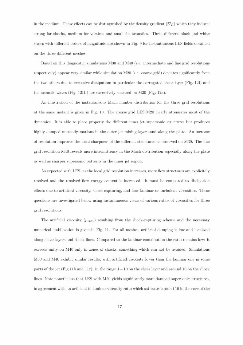
Time-averaged static pressure distributions on the impinging wall are given on Fig. 14a. It shows
a very good grid convergence between simulations M20, M30, and M40. The pressure fluctuation,
on Fig. 14b, shows the same convergence, except for the peaks at r = ±0.5d where simulation M40
exhibits fluctuations which are 20% higher than simulation M30.
First-order moments for velocity and pressure show satisfactory agreement with respect to grid
resolution (Fig. 13a, 13b, and 14a): a first-order convergence is achieved. Second-order moments
converge too but more slowly in the recirculation bubble.
21
r/d
-2-4 0
0
2 4
1.105
2.105
3.105
<p
>m
ea
n[P
a]
r/d
-2-4 0
0
2 4
1.104
3.104
5.104
<p
>rm
s[P
a]
M20M30M40
a) Mean pressure b) R.M.S. pressure
Fig. 14 Pressure profile at the wall
3. Spectral Analysis
The energy content of the resolved scales can be quantified by means of spectral estimators to
investigate the evolution of the energy distribution with respect to the grid resolution.
A common first-order spectral estimator is the Sound Pressure Level (SPL) distribution of a
pressure signal versus the frequency f . For a location ~x, the pressure signal is sampled each 10µs for
ten different radial directions in ~y~z planes. The following results are averaged azimuthally over these
10 locations. This averaging process is denoted <>az.. The Fourier transform of pressure is denoted
px. Note that this transformation involves chronologically i) a resampling of the datasets to ensure
a fixed time step, ii) a removal of the linear trends, iii) a low-pass filtering removing frequencies
above 40% times the Nyquist frequency, iv) Hanning windowing. The windowing is done for the
ten locations before azimuthal averaging <>az.. The Nyquist frequency approaches 100 kHz for all
signals. Care has been taken that all segments present the same first and second statistical moments
within a 10% tolerance. With the adequate normalization, the norm of the Fourier transform gives
the amplitude of each harmonic depending on the frequency Ax(f), Eq. (6). Sound pressure level
is defined as the root mean square of each harmonic normalized by the reference 20 µPa, and often
expressed in decibels, as in Eq. (7).
Ax(f) ≡⟨√
pxpx∗
⟩az.
(6)
22
SPLx(f) ≡ 20 log
(Ax ×
√2/2
20 µPa
)(7)
’Impact’(4.160.5
)
’Middle’(2.080.5
)’Lip’
(0.10.5
)
’Acoustic’(2.52.5
)
’Impact’,’Middle’,’Lip’
’Acoustic’
Front viewSide view
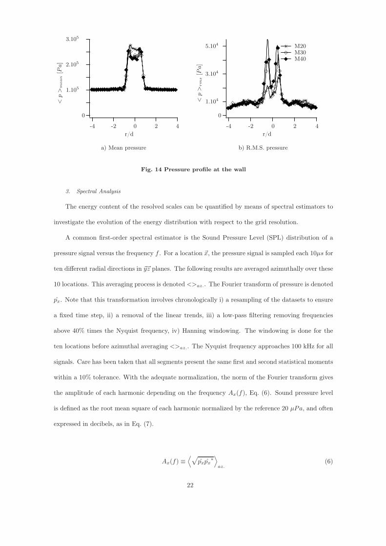
Fig. 15 Locations used for spectral analysis. Coordinates are specified as(
x/d
r/d
).
The spectrum is built for four different locations,’Impact’,’Middle’,’Lip’, and ’Acoustic’, detailed
in Fig. 15. Going from the highest to the lowest energy content, the spectral analysis yields :
1. ’Impact’ : on the impact plate (Fig. 16a) where the strongest pressure fluctuations occur. SPL
is abvove 160 dB in the range 0− 10 kHz. A weak maximum is found for both mesh M30 and
M40 at the frequency 6 kHz, corresponding to a RMS fluctuation near 4000 Pa. The energy
content decreases slowly for the high frequencies.
2. ’Middle’ : in the middle of the jet, near the Mach disc (Fig. 16b), the energy content is almost
constant near 140 dB, i.e. a RMS fluctuation around 200 Pa.
3. ’Lip’ : at the nozzle lip (Fig. 16c), the maximum energy starts at 140 dB in the lowest frequency
range and decreases smoothly towards 120 dB for 25 kHz (100 dB for mesh M20).
4. ’Acoustic’: In the zone at rest, to isolate propagating acoustic waves (Fig. 16d), the energy
distribution is comparable to the impact zone. The SPL rises in the range 0 − 6 kHz from
100 dB to 140 dB, then decreases on the range 6 − 20 kHz down to 120 dB (110 dB for mesh
M20).
23

The spectra are very different in terms of energy distribution and amplitude (Fig. 16). However
a clear convergence is established between simulations M30 and M40. The simulation M20 shows in
all cases an energetic content 10 dB lower than the two finer grids. The most important discrepancy
between simulation M30 an M40 is observed in the impact region, Fig. 16a with a shift of 3 dB/Hz.
This shift can be linked to the pressure fluctuations, stronger with the simulation M40. This
discrepancy has no impact on the energy spectra at the three other locations. In spite of a maximum
amplitude reached for 6 kHz, there is no discrete tone production in this case, as expected from
experiments.
Freq. [Hz]
0
100
120
140
160
180
5000 10000 15000 20000 25000
SP
L[d
B]
Freq. [Hz]
0
100
120
140
160
180
5000 10000 15000 20000 25000
SP
L[d
B]
a) ’Impact’ b) ’Middle’
Freq. [Hz]
0
100
120
140
160
180
5000 10000 15000 20000 25000
SP
L[d
B]
Freq. [Hz]
0
100
120
140
160
180
5000 10000 15000 20000 25000
SP
L[d
B]
M20M30M40
c) ’Lip’ d) ’Acoustic’
Fig. 16 Averaged Energy spectra
Involving non-linear products, the two-points estimators are part of second-order spectral anal-
yses. The interspectrum Sxy between the pressure signals of locations ~x and ~y is normalized by the
24

source energy Sxx, yielding the coherence estimator:
Cohxy ≡⟨ |Sxy|2|Sxx|2
⟩
az.
≡⟨ |pxpy
∗|pxpx
∗
⟩
az.
(8)
This quantity equals one when the target signal py shows the same amplitude and frequency as the
source signal px. Note that such tools are subject to signal to noise sensitivity: coherence between
a signal and a white noise showing the same fluctuations amplitude leads to a coherence near unity.
As we are dealing with signals of very different amplitudes (cf. Fig 16), the coherence average level
is expected to be low. To compare with the SPL levels, the coherence will be expressed in dB. The
phase of the interspectrum Φxy defined in Eq. (9) gives the time shift between the signals:
Φxy ≡ Φ 〈Sxy〉az. ≡ 〈pxpy∗〉az. (9)
Note that when two signals are strongly correlated at all frequencies, the time shift is a linear
function of the frequency. The slope of this linear function depends on the propagation speed of the
signal and the distance between the two locations.
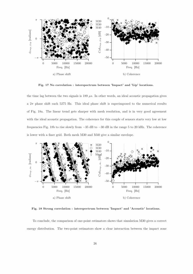
These tools are first applied to a couple of sensors showing almost no correlation. The fluc-
tuations on the wall at the edge of the reciculation zone are probably one of the strong acoustic
sources in this flow. As there is no discrete tone production, the response of the jet to acoustics
is expected to be low. Therefore, the locations ’Impact’ and ’Lip’ are expected to be uncorrelated.
The two-point phase estimator shown on Fig. 17a shows stricly no linear trend between the two
locations. The coherence estimator illustrated on Fig. 17b starts near unity (−0 dB) in the very
low frequency range and quickly reaches an enveloppe between −20 dB and −30 dB for all three
simulations. This quantity shows the difference of SPL between ’Lip’ and ’Impact’ region (difference
between Fig. 16a and 16c). Note that coherence seems to get lower with mesh refinement. However,
the results are globally independent of the grid.
The two-point estimators are then applied to a couple of locations expected to be strongly
correlated. Indeed, the ’Acoustic’ location must be directly perturbated by the ’Impact’ zone. A
clear linear trend is visible on Fig. 18a. The linear slope is roughly estimated by a phase shift of 2π
radians each 5000 Hz. This can be compared to an ideal acoustic propagation. The distance between
the two locations is 65.96 mm and the sound propagates at a constant velocity of 347 m/s. Therefore,
25
Freq. [Hz]
0
0
π
−π
5000 10000 15000 20000
M20M30M40
φIm
p.,
Lip
[radia
ns]
Freq. [Hz]
5000 10000 15000 20000
Coh
Im
p.,
Lip
[dB
]
0
0
-10
-20
-30
-40
-50
a) Phase shift b) Coherence
Fig. 17 No correlation : interspectrum between ’Impact’ and ’Lip’ locations.
the time lag between the two signals is 189 µs. In other words, an ideal acoustic propagation gives
a 2π phase shift each 5275 Hz. This ideal phase shift is superimposed to the numerical results
of Fig. 18a. The linear trend gets sharper with mesh resolution, and is in very good agreement
with the ideal acoustic propagation. The coherence for this couple of sensors starts very low at low
frequencies Fig. 18b to rise slowly from −35 dB to −30 dB in the range 5 to 20 kHz. The coherence
is lower with a finer grid. Both mesh M30 and M40 give a similar envelope.
Freq. [Hz]
0
0
π
−π
5000 10000 15000 20000
M20M30M40Ideal
φIm
p.,
Ac.[radia
ns]
Freq. [Hz]
5000 10000 15000 20000
Coh
Im
p.,
Ac.[d
B]
0
0
-10
-20
-30
-40
-50
a) Phase shift b) Coherence
Fig. 18 Strong correlation : interspectrum between ’Impact’ and ’Acoustic’ locations.
To conclude, the comparison of one-point estimators shows that simulation M30 gives a correct
energy distribution. The two-point estimators show a clear interaction between the impact zone
26

and the acoustic field, in spite of a large difference of intensity between the two signals (30 dB).
Moreover, one and two-point estimators results are unchanged betweed meshes M30 and M40.
V. Conclusion and perspectives
LES of a supersonic jet impinging on a flat plate in a stable regime have been performed
with an explicit third-order compressible solver using an unstructured mesh and the Smagorinsky
model. Simulations showed a satisfactory agreement with experiment observations. Three levels
of mesh refinement were compared in terms of instantaneous and averaged flow fields (shocks and
recirculation zone positions), averaged flow velocity and pressure fields, wall pressure, RMS pressure
fields, spectral content. The mid and high-resolution grids yield almost the same results, especially
for one- and two-point spectral analyses. The effects of numerical dissipation and turbulent viscosity
are also compared on the three grids and shown to be well controlled. The finest grid used here (a
22 Mcell mesh) is sufficient to ensure grid-independent results and offer a coherent framework to use
LES to investigate more complex mechanisms on this type of flow, for example self-excited tones.
Acknowledgements
Authors acknowledge the ’GENCI Grand Challenge 2009’ team of the CEA for making available
the Bull hybrid computer ’titane’ ressources and G. Staffelbach for his technical support in porting
the AVBP solver on this new architecture. Authors wish to thanks A. Sevrain of IMFT for his
contribution on spectral analysis, and B. Henderson for the information and experimental data
provided for this study.
References
[1] Roux, A., Reichstadt, S., Bertier, N., Gicquel, L. Y. M., Vuillot, F., and Poinsot, T., “Comparison of
numerical methods and combustion models for LES of a ramjet,” C. R. Acad. Sci. Mécanique, Vol. 337,
No. 6-7, 2009, pp. 352–361.
[2] Wolf, P., Staffelbach, G., Roux, A., Gicquel, L., Poinsot, T., and Moureau, V., “Massively parallel
LES of azimuthal thermo-acoustic instabilities in annular gas turbines,” C. R. Acad. Sci. Mécanique,
Vol. 337, No. 6-7, 2009, pp. 385–394.
27
[3] Roux, S., Cazalens, M., and Poinsot, T., “Influence of Outlet Boundary Condition for Large Eddy
Simulation of Combustion Instabilities in Gas Turbine,” J. Prop. Power , Vol. 24, No. 3, 2008, pp. 541–
546.
[4] Staffelbach, G., Gicquel, L., Boudier, G., and Poinsot, T., “Large Eddy Simulation of self-excited
azimuthal modes in annular combustors,” Proc. Combust. Inst. , Vol. 32, 2009, pp. 2909–2916.
[5] James, S., Zhu, J., and Anand, M., “LES of turbulent flames using the filtered density function model,”
Proc. Combust. Inst. , Vol. 31, 2007, pp. 1737–1745.
[6] Inman, J. A. W., Danehy, P. M., Nowak, R. J., and Alderfer, D. W., “Fluorescence Imaging Study of
Impinging Underexpanded Jets,” 46th AIAA Aerospace Sciences Meeting and Exhibit, 2008.
[7] Henderson, B., Bridges, J., and Wernet, M., “An Experimental Study of the Oscillatory Flow Structure
of Tone-Producing Supersonic Impinging Jets,” J. Fluid Mech. , Vol. 542, 2005, pp. 115–137.
[8] Henderson, B. and Powell, A., “Sound-production mechanisms of the axisymmetric choked jet impinging
on small plates: The production of primary tones,” J. Acous. Soc. Am. , Vol. 99, 1996, pp. 153.
[9] Henderson, B., “The connection between sound production and jet structure of the supersonic impinging
jet,” J. Acous. Soc. Am. , Vol. 111, 2002, pp. 735.
[10] Donaldson, C. D. and Snedeker, R. S., “A Study of Free Jet Impingement. Part 1. Mean Properties of
Free and Impinging Jets,” J. Fluid Mech. , Vol. 45, 1971, pp. 281–319.
[11] Donaldson, C. D., Snedeker, R. S., and Margolis, D. P., “A Study of Free Jet Impingement. Part 2. Free
Jet Turbulent Structure and Impingement Heat Transfer,” J. Fluid Mech. , Vol. 45, 1971, pp. 477–512.
[12] Lamont, P. J. and Hunt, B. L., “The Impingement of Underexpanded, Axisymmetric Jets on Perpen-
dicular and Inclined Flat Plates,” J. Fluid Mech. , Vol. 100, 1980, pp. 471–511.
[13] Ho, C.-M. and Nosseir, N. S., “Dynamics of an Impinging Jet. Part 1. The Feedback Phenomenon,”
J. Fluid Mech. , Vol. 105, 1981, pp. 119–142.
[14] Kuo, C.-Y. and Dowling, A. P., “Oscillations of a Moderately Underexpanded Choked Jet Impinging
Upon a Flat Plate,” J. Fluid Mech. , Vol. 315, 1996, pp. 267–291.
[15] Berland, J., Bogey, C., and Bailly, C., “Numerical study of screech generation in a planar supersonic
jet,” Phys. Fluids , Vol. 19, 2007, pp. 075105.
[16] Larchevêque, L., Sagaut, P., Le, T., and Comte, P., “Large-eddy simulation of a compressible flow in a
three-dimensional open cavity at high Reynolds number,” J. Fluid Mech. , Vol. 516, 2004, pp. 265–301.
[17] Ferri, A., Elements of aerodynamics of supersonic flows, Macmillan Co., 1949.
[18] Adamson, T. C., “Approximate methods for calculating the structure of jets from highly underexpanded
nozzles,” Tech. rep., BAMIRAC, 1961.
28

[19] Hsu, A. and Liou, M., “Computational analysis of underexpanded jets in the hypersonic regime,”
J. Prop. Power , Vol. 7, 1991, pp. 297–299.
[20] Birkby, P., Dent, J., and Page, G., “CFD Prediction of Turbulent Sonic Underexpanded Jets,” Proceed-
ings of the 1996 ASME Fluids Engineering Summer Meeting Pt. 2 , ASME, ASME, 1996, pp. 465–470.
[21] Cumber, P., Fairweather, M., Falle, S., and Giddings, J., “Predictions of the structure of turbulent,
highly underexpanded jets,” J. Fluids Eng. , Vol. 117, 1995, pp. 599–604.
[22] Gribben, B. J., Badcock, K. J., and Richards, B. E., “Numerical Study of Shock-Reflection Hysteresis
in an Underexpanded Jet,” AIAA Journal , Vol. 38, 2000, pp. 275–283.
[23] Prudhomme, S. and Haj-Hariri, H., “Investigation of supersonic underexpanded jets using adaptive
unstructured finite elements,” Finite Elem. Anal. Des. , Vol. 17, No. 1, 1994, pp. 21–40.
[24] Sakakibara, Y. and Iwamoto, J., “Numerical Study of Oscillation Mechanism in Underexpanded Jet
Impinging on Plate,” J. Fluids Eng. , Vol. 120, 1998, pp. 477.
[25] Alvi, F. S., Ladd, J. A., and Bower, W. W., “Experimental and Computational Investigation of Super-
sonic Impinging Jets,” AIAA Journal , Vol. 40, 2002, pp. 599–609.
[26] Shen, H. and Tam, C. K. W., “Three-Dimensional Numerical Simulation of the Jet Screech Phe-
nomenon,” AIAA Journal , Vol. 40, 2002, pp. 33–41.
[27] Arunajatesan, S. and Sinha, N., “Large Eddy Simulations of Supersonic Impinging Jet Flow Fields,”
AIAA Paper , Vol. 4287, 2002, pp. 2002.
[28] Berland, J., Bogey, C., and Bailly, C., “Large eddy simulation of screech tone generation in a planar
underexpanded jet,” 12th AIAA/CEAS Aeroacoustics Conference, 2006, pp. 8–10.
[29] Al-Qadi, I. and Scott, J., “High-order three-dimensional numerical simulation of a supersonic rectan-
gular jet,” AIAA Paper , Vol. 3238, 2003, pp. 2003.
[30] Bodony, D. J. and Lele, S. K., “On using large-eddy simulation for the prediction of noise from cold
and heated turbulent jets,” Phys. Fluids , Vol. 17, 2005.
[31] Bogey, C. and Bailly, C., “Computation of a high Reynolds number jet and its radiated noise using
large eddy simulation based on explicit filtering,” Comput. Fluids , Vol. 35, 2006, pp. 1344–1358.
[32] Bogey, C. and Bailly, C., “Investigation of downstream and sideline subsonic jet noise using Large Eddy
Simulations.” Theoret. Comput. Fluid Dynamics , Vol. 20, No. 1, 2006, pp. 23–40.
[33] Georgiadis, N., Alexander, J., and Reshotko, E., “Hybrid Reynolds-averaged Navier-Stokes/large-eddy
simulations of supersonic turbulent mixing,” AIAA Journal , Vol. 41, No. 2, 2003, pp. 218–229.
[34] Chauvet, N., Deck, S., and Jacquin, L., “Shock patterns in a slightly underexpanded sonic jet controlled
by radial injections,” Phys. Fluids , Vol. 19, 2007, pp. 048104.
29
[35] Piomelli, U., “Wall-layer models for large-eddy simulations,” Prog. Aerospace Sci. , Vol. 44, No. 6,
2008, pp. 437–446.
[36] Georgiadis, N., Alexander, J., and Reshotko, E., “Development of a hybrid RANS/LES method for
compressible mixing layer simulations,” AIAA Paper , Vol. 41, 2001, pp. 218–229.
[37] Cheng, T. and Lee, K., “Numerical simulations of underexpanded supersonic jet and free shear layer
using WENO schemes,” Int. J. Heat Fluid Flow , Vol. 26, No. 5, 2005, pp. 755–770.
[38] Chauvet, N., Deck, S., and Jacquin, L., “Zonal Detached Eddy Simulation of a Controlled Propulsive
Jet,” AIAA Journal , Vol. 45, No. 10, 2007, pp. 2458.
[39] Chauvet, N., Deck, S., and Jacquin, L., “Numerical Study of Mixing Enhancement in a Supersonic
Round Jet,” AIAA Journal , Vol. 45, No. 7, 2007, pp. 1675.
[40] Singh, A. and Chatterjee, A., “Numerical prediction of supersonic jet screech frequency,” Shock Waves
, Vol. 17, No. 4, 2007, pp. 263–272.
[41] Deck, S., “Delayed detached eddy simulation of the end-effect regime and side-loads in an overexpanded
nozzle flow,” Shock Waves , Vol. 19, No. 3, 2009, pp. 239–249.
[42] Powell, A., “The sound-producing oscillations of round underexpanded jets impinging on normal plates,”
J. Acous. Soc. Am. , Vol. 83, No. 2, 1988, pp. 515–533.
[43] Courant, R., Isaacson, E., and Rees, M., “On the solution of non linear hyperbolic differential equations
by finite differences,” Commun. Pure Appl. Math. , Vol. 5, 1952.
[44] Donea, J., “A Taylor-Galerkin method for convective transport problems,” Int. J. Numer. Meth. Eng.
, Vol. 20, No. 1, 1984.
[45] Favre, A., “Problems of Hydrodynamics and Continuum Mechanics,” Soc. Indust. Appl. Mech. , 1969.
[46] Sagaut, P., Large eddy simulation for incompressible flows, Springer, 2002.
[47] Ferziger, J. H. and Perić, M., Computational Methods for fluid Dynamics, Springer, 3rd ed., 2002.
[48] Pope, S. B., Turbulent flows, Cambridge University Press, 2000.
[49] Smagorinsky, J., “General circulation experiments with the primitive equations: 1. The basic experi-
ment.” Mon. Weather Rev. , Vol. 91, 1963, pp. 99–164.
[50] Germano, M., “Turbulence: the filtering approach,” J. Fluid Mech. , Vol. 238, 1992, pp. 325–336.
[51] Ghosal, S. and Moin, P., “The basic equations for the large eddy simulation of turbulent flows in complex
geometry,” J. Comput. Phys. , Vol. 118, 1995, pp. 24 – 37.
[52] Meneveau, C., Lund, T., and Cabot, W., “A lagrangian dynamic subgrid-scale model of turbulence,”
J. Fluid Mech. , Vol. 319, 1996, pp. 353.
[53] Moin, P., Squires, K. D., Cabot, W., and Lee, S., “A dynamic subgrid-scale model for compressible
30
turbulence and scalar transport,” Phys. Fluids , Vol. A 3, No. 11, 1991, pp. 2746–2757.
[54] Lilly, D. K., “A proposed modification of the germano sub-grid closure method,” Phys. Fluids , Vol. 4,
No. 3, 1992, pp. 633–635.
[55] Boyaval, S. and Dumouchel, C., “Deconvolution technique to determine local spray drop size
distributions—application to high-pressure swirl atomizers,” ILASS-Europe, Zurich, 2001.
[56] Gicquel, L., Givi, P., Jaberi, F., and Pope, S., “Velocity filtered density function for large eddy simu-
lation of turbulent flows,” Phys. Fluids , Vol. 14, 2002, pp. 1196.
[57] Fureby, C. and Grinstein, F. F., “Monotonically Integrated Large-Eddy Simulation of Free Shear Flows,”
AIAA Journal , Vol. 37, No. 5, 1999, pp. 544–556.
[58] Cook, A. and Cabot, W., “Hyperviscosity for shock-turbulence interactions,” J. Comput. Phys. ,
Vol. 203, No. 2, 2005, pp. 379–385.
[59] Jameson, A., Schmidt, W., and Turkel, E., “Numerical solution of the Euler equations by finite volume
methods using Runge-Kutta time stepping schemes,” AIAA Paper , Vol. 81-1259, 1981.
[60] von Neumann, J. and Richtmeyer, R. D., “A method for the numerical calculation of hydrodynamic
shocks,” J. Appl. Phys. , Vol. 21, 1950, pp. 231.
[61] Bogey, C., de Cacqueray, N., and Bailly, C., “A shock-capturing methodology based on adaptative
spatial filtering for high-order non-linear computations,” J. Comput. Phys. , Vol. 228, No. 5, 2009,
pp. 1447–1465.
[62] Cook, A. and Cabot, W., “A high-wavenumber viscosity for high-resolution numerical methods,”
J. Comput. Phys. , Vol. 195, No. 2, 2004, pp. 594–601.
[63] Jiang, G. S. and Shu, C. W., “Efficient implementation of weighted ENO schemes,” J. Comput. Phys.
, Vol. 126, 1996, pp. 202–228.
[64] Cook, Andrew, W. and Cabot, William, H., “A High-Wavenumber viscosity for high Resolution Nu-
merical Methods,” Tech. rep., Lawrence Livermore Nat. Lab., Feb 2003.
[65] Roux, A., Gicquel, L., Sommerer, Y., and Poinsot, T., “Large eddy simulation of mean and oscillating
flow in side-dump ramjet combustor,” Combust. Flame , Vol. 152, No. 1-2, 2008, pp. 154–176.
[66] Zapryagaev, V., Pickalov, V., Kiselev, N., and Nepomnyashchiy, A., “Combination Interaction of
Taylor–Goertler Vortices in a Curved Shear Layer of a Supersonic Jet,” Theoret. Comput. Fluid Dy-
namics , Vol. 18, No. 2, 2004, pp. 301–308.
[67] Zapryagaev, V., Kiselev, N., and Pavlov, A., “Effect of Streamline Curvature on Intensity of Streamwise
Vortices in the Mixing Layer of Supersonic Jets,” J. Appl. Mech. , Vol. 45, No. 3, 2004, pp. 335–343.
[68] Krothapalli, A., Strykowski, P., and King, C., “Origin of Streamwise Vortices in Supersonic Jets,”
31

AIAA Journal , Vol. 36, No. 5, 1998, pp. 869–872.
[69] Hussain, F. and Jeong, J., “On the identification of a vortex,” J. Fluid Mech. , Vol. 285, 1995, pp. 69–94.
[70] Pope, S. B., “Ten questions concerning the large-eddy simulation of turbulent flows,” New J. Phys. ,
Vol. 6, 2004, pp. 35.
[71] Senoner, J., Sanjosé, M., Lederlin, T., Jaegle, F., García, M., Riber, E., Cuenot, B., Gicquel, L., Pitsch,
H., and Poinsot., T., “Evaluation of numerical strategies for two-phase reacting flows,” C. R. Acad.
Sci. Mécanique, Vol. 337, No. 6-7, 2009, pp. 528–538.
[72] Metais, O. and Lesieur, M., “Statistical probability of decaying turbulence,” Journal of Atmospheric
Science, Vol. 43, 1986.
32


