Download - L Phy.electromagnetic Wave-Rusli
1
12. ELECTROMAGNETIC WAVES12.1 Maxwell’s Equations12.2 Plane Electromagnetic Waves12.3 Energy Carried by Electromagnetic Waves

2
12.1 Maxwell’s EquationsWe have encountered four key equations in electricity and magnetism.
These equations are collectively known as Maxwell’s equations.They are regarded as the basis to describe all electrical and magnetic phenomena.
magnetism inlaw sGauss'(12.2) 0
law sGauss'(12.1) 0
=⋅
=⋅
∫
∫AdB
qAdE in
vv
vv
ε
law Maxwell-Ampere(12.4)
law sFaraday'(12.3)
000 dtdIsdB
dtdsdE
E
B
Φ+=⋅
Φ−=⋅
∫
∫
µεµvv
vv
3
12.1 Maxwell’s EquationsGauss’s law:
The total electric flux through any closed surface equals the net charge enclosed by that surface divided by ε0 . It relates the electric field to the charge distribution that creates it.
Gauss’s law in magnetism:
The net magnetic flux through any closed surface is zero. The number of magnetic field lines that enter a closed volume must equal the number that leave that volume. This comes from the fact that magnetic field lines form closed loops.
0εinq
AdE =⋅∫vv
0=⋅∫ AdBvv

4
12.1 Maxwell’s EquationsFaraday’s law of induction:
The emf induced, which is the line integral of the electric field around any closed path, equals the rate of change of magnetic flux through any surface area bounded by that path.
It describes the creation of an electric field by a changing magnetic field. Current is induced in a conducting loop placed in a time-varying magnetic field.
∫Φ
−=⋅dt
dsdE Bvv
5
12.1 Maxwell’s EquationsAmpere-Maxwell law:
The line integral of the magnetic field around any closed path is the sum of µ0 times the net current through any surface bounded by that path and ε0 µ0 times the rate of change of electric flux through any surface bounded by that path. It describes the creation of a magnetic field by an electric current and a changing electric field.
Once the electric and magnetic fields are known at some point inspace, the force acting on a charged particle can be calculated from the Lorentz force law
Maxwell’s equations, together with the Lorentz force law, completely describe all classical electromagnetic interactions.
∫Φ
+=⋅dt
dIsdB E000 µεµvv
)5.12(BvqEqFvvvv
×+=
6
12.1 Maxwell’s EquationsIn vacuum where there are no charges or conduction currents, i.e. qin = I = 0, the Maxwell’s equations are reduced to
The perfect symmetry in the Faraday’s and Ampere-Maxwell’s laws shows that a time-varying field of either kind induces a field of the other kind.
)9.12(
)8.12(
)7.12(0
)6.12(0
00∫
∫
∫∫
Φ=⋅
Φ−=⋅
=⋅
=⋅
dtdsdB
dtdsdE
AdB
AdE
E
B
εµvv
vv
vv
vv

7
12.1 Maxwell’s EquationsAs shall be shown, the Maxwell’s equations predict the existence of wave, i.e. time-varying electric and magnetic fields that propagate through space. These are known as electromagnetic (EM) waves.
Radio and television waves, visible light, infrared, ultraviolet, X-rays, etc are all EM waves.
Before discussing EM waves, let’s revise the general mathematical description of a wave.

8
12.2 Plane Electromagnetic WavesA sinusoidal wave with a wavelength λ can be expressed as
If the wave travels along +ve x-axis with a speed ν, at any time t, it can be expressed as
The wave travels a distance of λ in one period T. Thus its speed ν is given by
Therefore,
)10.12(2sin ⎟⎠⎞
⎜⎝⎛= xAyλπ
)11.12()(2sin ⎟⎠⎞
⎜⎝⎛ −= txAy υλπ
)12.12(Tλυ =
)13.12()(2sin ⎟⎠⎞
⎜⎝⎛ −=
TtxAy
λπ
9
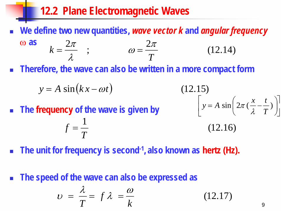
12.2 Plane Electromagnetic WavesWe define two new quantities, wave vector k and angular frequency ω as
Therefore, the wave can also be written in a more compact form
The frequency of the wave is given by
The unit for frequency is second-1, also known as hertz (Hz).
The speed of the wave can also be expressed as
)14.12(2;2T
k πωλπ
==
( ) )15.12(sin txkAy ω−=
)16.12(1T
f =
)17.12(k
fT
ωλλυ ===
⎥⎦
⎤⎢⎣
⎡⎟⎠⎞
⎜⎝⎛ −= )(2sin
TtxAy
λπ

10
12.2 Plane Electromagnetic WavesSolving for the Maxwell’s equations can be very complicated. Forsimplicity, we shall consider only linearly polarised EM waves. These are waves in which the electric and magnetic fields are oscillating on two perpendicular planes.
For example, we can have an EM wave travelling in the x direction, with the electric field E oscillating in the y direction and the magnetic field B oscillating in the z direction. Such waves are also called plane waves.
11
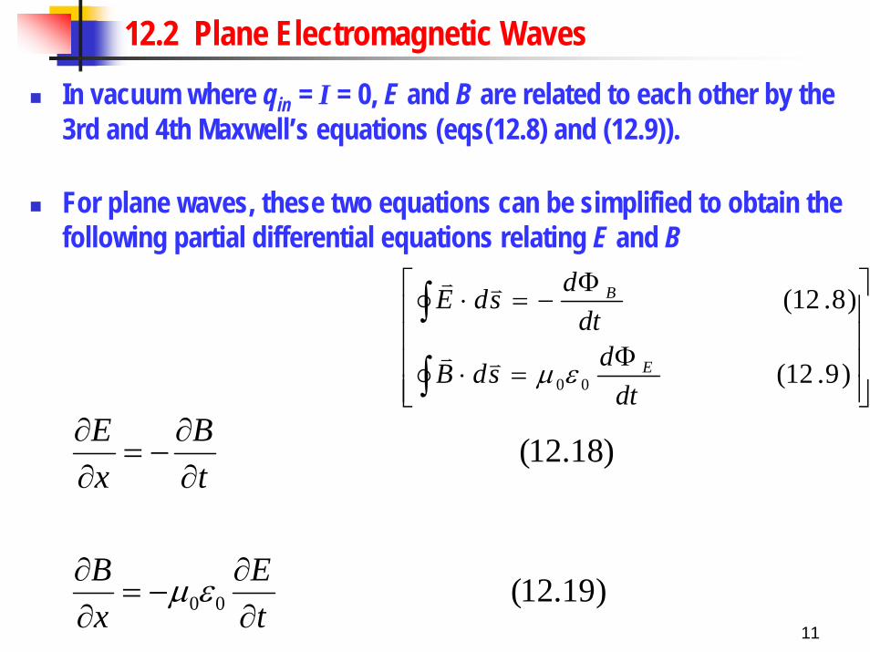
12.2 Plane Electromagnetic WavesIn vacuum where qin = I = 0, E and B are related to each other by the 3rd and 4th Maxwell’s equations (eqs(12.8) and (12.9)).
For plane waves, these two equations can be simplified to obtain the following partial differential equations relating E and B
)19.12(
)18.12(
00 tE
xB
tB
xE
∂∂
−=∂∂
∂∂
−=∂∂
εµ
⎥⎥⎥⎥
⎦
⎤
⎢⎢⎢⎢
⎣
⎡
Φ=⋅
Φ−=⋅
∫
∫
)9.12(
)8.12(
00 dtdsdB
dtdsdE
E
B
εµvv
vv

12
12.2 Plane Electromagnetic WavesPartial differentiate eq(12.18) with respect to x gives
Substitute eq(12.19) into the above equation,
Similarly
⎥⎥⎥⎥
⎦
⎤
⎢⎢⎢⎢
⎣
⎡
∂∂
−=∂∂
∂∂
−=∂∂
)19.12(
)18.12(
00 tE
xB
tB
xE
εµ
⎟⎠⎞
⎜⎝⎛∂∂
∂∂
−=⎟⎠⎞
⎜⎝⎛∂∂
∂∂
−=∂∂
xB
ttB
xxE2
2
(12.20) 2
2
002
2
002
2
tE
xE
tE
txE
∂∂
=∂∂
⎟⎠⎞
⎜⎝⎛
∂∂
−∂∂
−=∂∂
εµ
εµ
(12.21) 2
2
002
2
tB
xB
∂∂
=∂∂ εµ
13
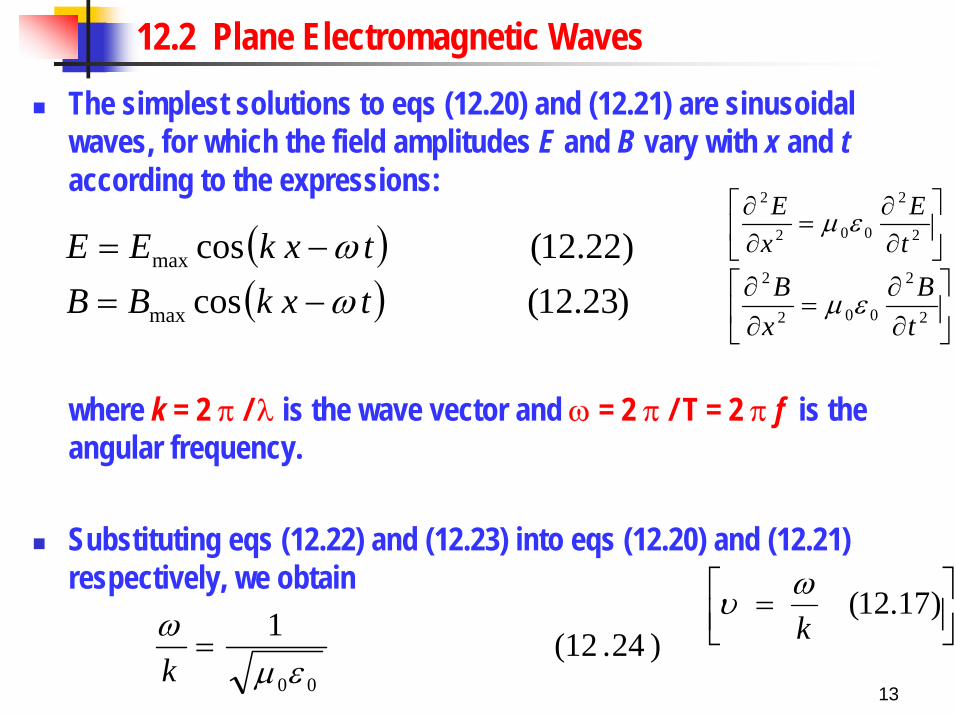
12.2 Plane Electromagnetic WavesThe simplest solutions to eqs (12.20) and (12.21) are sinusoidal waves, for which the field amplitudes E and B vary with x and taccording to the expressions:
where k = 2 π / λ is the wave vector and ω = 2 π / T = 2 π f is theangular frequency.
Substituting eqs (12.22) and (12.23) into eqs (12.20) and (12.21) respectively, we obtain
( )( ) )23.12(cos
)22.12(cos
max
max
txkBBtxkEE
ωω
−=−=
)24.12(1
00εµω
=k
⎥⎦
⎤⎢⎣
⎡∂∂
=∂∂
2
2
002
2
tB
xB εµ
⎥⎦
⎤⎢⎣
⎡∂∂
=∂∂
2
2
002
2
tE
xE εµ
⎥⎦⎤
⎢⎣⎡ = )17.12(
kωυ

14
12.2 Plane Electromagnetic WavesUsing eq(12.17), the speed of the EM wave in vacuum is deduced to be
The value of c can be calculated
This is precisely the same as the speed of light in vacuum.
Conclusion: Light is an electromagnetic wave.
)25.12(1
00εµ=c
( ) ( )
smc
mNCAmTc
/1099792.2
/1085419.8/1041
8
22127
×=
⋅×⋅×=
−−π
15
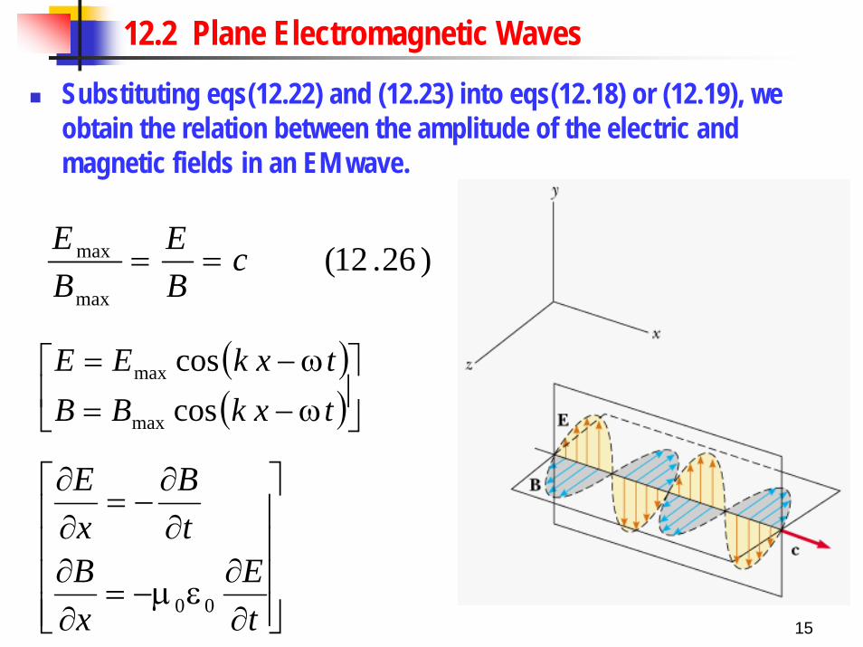
12.2 Plane Electromagnetic WavesSubstituting eqs(12.22) and (12.23) into eqs(12.18) or (12.19), we obtain the relation between the amplitude of the electric and magnetic fields in an EM wave.
)26.12(max
max cBE
BE
==
( )( )⎥⎦
⎤⎢⎣
⎡ω−=ω−=
txkBBtxkEE
coscos
max
max
⎥⎥⎥⎥
⎦
⎤
⎢⎢⎢⎢
⎣
⎡
∂∂
εµ−=∂∂
∂∂
−=∂∂
tE
xB
tB
xE
00

16
12.2 Plane Electromagnetic WavesProperties of EM wavesThe electric and magnetic fields fluctuate sinusoidally in time. They are perpendicular to each other and perpendicular to the direction of wave propagation. Thus, EM waves are transverse waves.
The cross product E x B gives the direction of travel of the wave.

17
12.2 Plane Electromagnetic WavesThe magnitudes of E and B in free space are related by E/B = c.
EM waves obey the principle of superposition.
EM waves are characterized by their wavelengths (or frequencies).

18
12.2 Plane Electromagnetic WavesThe EM waves of different wavelengths made up the electromagnetic spectrum. The visible light occupies only a small region of the entire spectrum.
All EM waves, no matter where they lie in the spectrum, travel through vacuum with the same speed c.

19
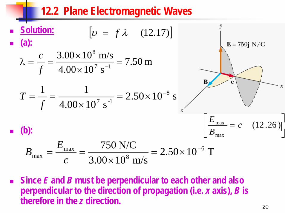
12.2 Plane Electromagnetic WavesExample 12.1: An electromagnetic waveA sinusoidal electromagnetic wave of frequency 40.0 MHz travels in free space in the x direction. (a) Determine the wavelength λ and period T of the wave. (b) At some point and at some time, the electric field has its maximum value of 750 N/C and is along the y axis. Calculate the magnitude and direction of the magnetic field at this position and time. (c) Write the expressions for the space-time variation of the components of the electric and magnetic fields for this wave.
20
12.2 Plane Electromagnetic WavesSolution:(a):
(b):
Since E and B must be perpendicular to each other and also perpendicular to the direction of propagation (i.e. x axis), B is therefore in the z direction.
T 1050.2m/s103.00
N/C 750 68
maxmax
−×=×
==c
EB
m 50.7s 1000.4m/s 1000.3
17
8
=××
==λ −fc
s 1050.2s 1000.4
11 81-7
−×=×
==f
T
[ ])17.12(λυ f=
⎥⎦
⎤⎢⎣
⎡= )26.12(
max
max cBE

21
12.2 Plane Electromagnetic Waves(c):
where
( ) ( ) ( )( ) ( ) ( )tkxtkxBB
tkxtkxEE
ω−×=ω−=
ω−=ω−=− cosT 1050.2cos
cosN/C 750cos6
max
max
( )rad/m 838.0
m5.722k
rad/s 1051.2s 1000.422 8-17
===
×=×==π
λπ
ππω f

22
12.3 Energy Carried By Electromagnetic WavesEM waves propagate through space, carrying energy and transferring it to objects in their paths.
The energy is carried by both the electric and magnetic fields that comprise the wave.
The energy carried by an EM wave is given by the Poynting vector S.
The direction of the Poynting vector Sgives the direction of energy transport. (Fig. 34.7)
)27.12(1
0
BESvvv
×≡µ
Fig.34.7

23
12.3 Energy Carried By Electromagnetic WavesThe magnitude of the Poynting vector S represents the rate of energy flow per unit area in the direction of wave propagation. (unit: J/s⋅m2 or W/m2)
For a plane electromagnetic wave where Eis perpendicular to B, the magnitude of S is given by
Since E/B = c, S can also be expressed as
)28.12(00 µµBEBE
S =×
=
vv
( ) )29.12(/ 2
00
2
00
Bcc
EcEEEBSµµµµ
====
24
12.3 Energy Carried By Electromagnetic WavesSince E and B are sinusoidal functions, the energy flow is not constant in time.
These equations for S at any instant of time represent the instantaneous rate at which energy is transferred per unit area.
Since the frequencies are usually so high that the rapid time variations of E and B are impossible to detect, the instantaneous values of S are only of theoretical interest.
A more useful quantity for the wave energy is the time average of S over one or more cycles, also known as the wave intensity I.
The intensity I gives the average power transferred per unit area.
⎥⎦
⎤⎢⎣
⎡µ
=0
BES
25
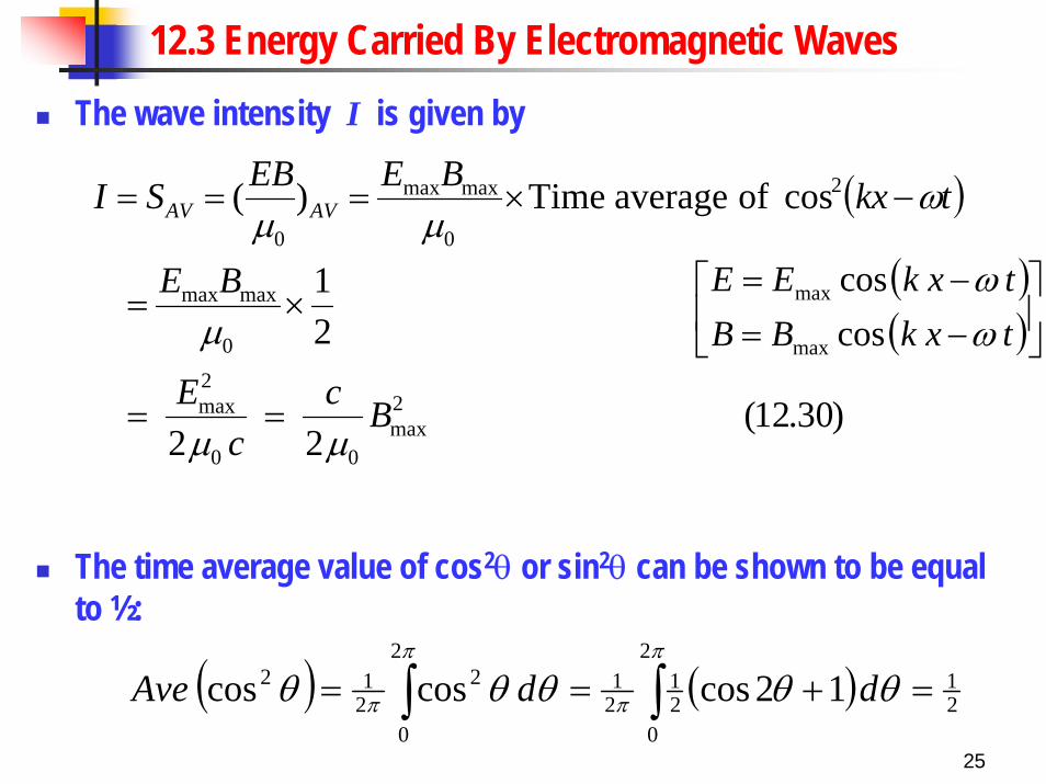
12.3 Energy Carried By Electromagnetic WavesThe wave intensity I is given by
The time average value of cos2θ or sin2θ can be shown to be equal to ½:
( )
)30.12(22
21
cos of average Time)(
2max
00
2max
0
maxmax
2
0
maxmax
0
Bcc
E
BE
tkxBEEBSI AVAV
µµ
µ
ωµµ
==
×=
−×===
( ) ( ) 21
2
021
21
2
0
2212 12coscoscos =+== ∫∫
π
π
π
π θθθθθ ddAve
( )( )⎥⎦
⎤⎢⎣
⎡−=−=
txkBBtxkEE
ωω
coscos
max
max
26
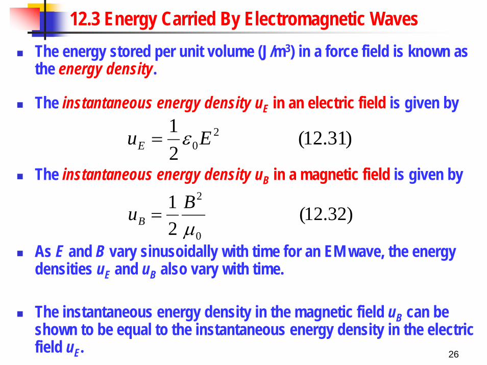
12.3 Energy Carried By Electromagnetic WavesThe energy stored per unit volume (J/m3) in a force field is known as the energy density.
The instantaneous energy density uE in an electric field is given by
The instantaneous energy density uB in a magnetic field is given by
As E and B vary sinusoidally with time for an EM wave, the energy densities uE and uB also vary with time.
The instantaneous energy density in the magnetic field uB can be shown to be equal to the instantaneous energy density in the electric field uE.
)31.12(21 2
0EuE ε=
)32.12(21
0
2
µBuB =
27
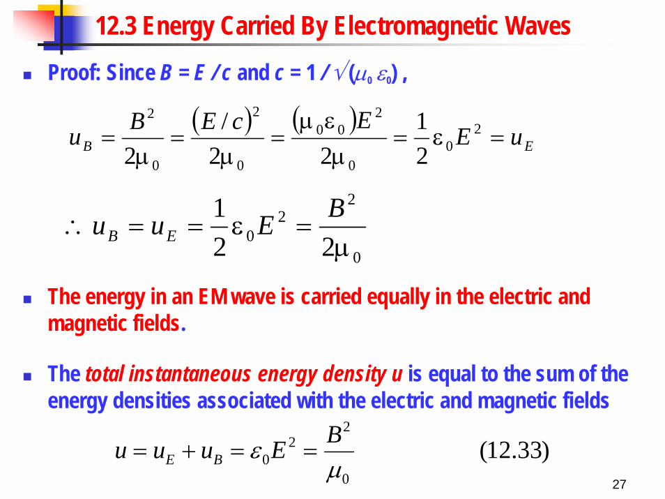
12.3 Energy Carried By Electromagnetic WavesProof: Since B = E / c and c = 1 / √ (µ0 ε0) ,
The energy in an EM wave is carried equally in the electric and magnetic fields.
The total instantaneous energy density u is equal to the sum of the energy densities associated with the electric and magnetic fields
( ) ( )EB uE
EcEBu =ε=µεµ
=µ
=µ
= 20
0
200
0
2
0
2
21
22/
2
0
22
0 221
µ=ε==∴
BEuu EB
)33.12(0
22
0 µε BEuuu BE ==+=
28
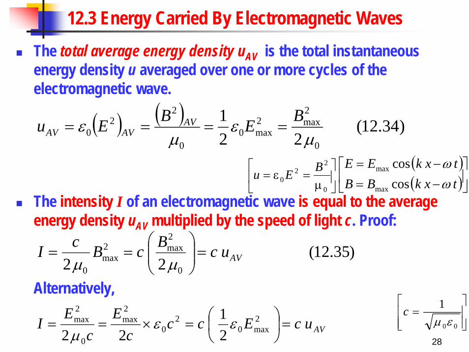
12.3 Energy Carried By Electromagnetic WavesThe total average energy density uAV is the total instantaneous energy density u averaged over one or more cycles of the electromagnetic wave.
The intensity I of an electromagnetic wave is equal to the average energy density uAV multiplied by the speed of light c. Proof:
Alternatively,
( ) ( ) )34.12(22
1
0
2max2
max00
22
0 µε
µε BEBEu AV
AVAV ====
)35.12(22 0
2max2
max0
AVucBcBcI =⎟⎟⎠
⎞⎜⎜⎝
⎛==
µµ
AVucEccc
Ec
EI =⎟
⎠⎞
⎜⎝⎛=×== 2
max02
0
2max
0
2max
21
22εε
µ⎥⎥⎦
⎤
⎢⎢⎣
⎡=
00
1εµ
c
⎥⎦
⎤⎢⎣
⎡µ
=ε=0
22
0BEu
( )( )⎥⎦
⎤⎢⎣
⎡−=−=
txkBBtxkEE
ωω
coscos
max
max
29
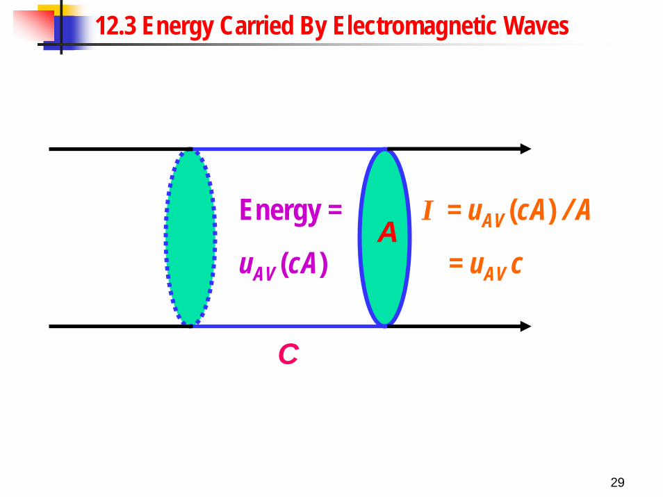
12.3 Energy Carried By Electromagnetic Waves
Energy =
uAV (cA)
I = uAV (cA) / A
= uAV cA
C
30
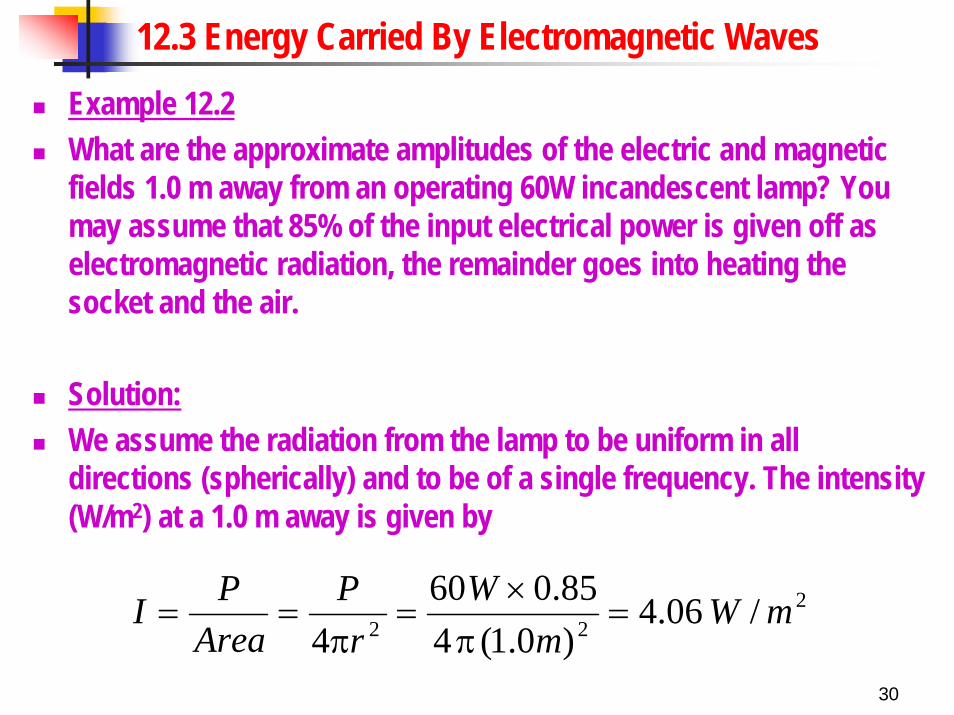
12.3 Energy Carried By Electromagnetic WavesExample 12.2What are the approximate amplitudes of the electric and magneticfields 1.0 m away from an operating 60W incandescent lamp? You may assume that 85% of the input electrical power is given off as electromagnetic radiation, the remainder goes into heating the socket and the air.
Solution:We assume the radiation from the lamp to be uniform in all directions (spherically) and to be of a single frequency. The intensity (W/m2) at a 1.0 m away is given by
222 /06.4
)0.1(485.060
4mW
mW
rP
AreaPI =
π×
=π
==

31
12.3 Energy Carried By Electromagnetic WavesFrom eq(12.30)
Since Emax/Bmax = c,
( )( )
mVsmATmmW
cIE o
/3.55/103/1042/06.4
2872
max
=
×××π×=
µ=−
Tsm
mVc
EB 7
8max
max 1084.1/100.3
/3.55 −×=×
==
⎥⎦
⎤⎢⎣
⎡=
cEI
0
2max
2µ


