Wayne State University
Wayne State University Theses
1-1-2016
Kinematic Modeling Of An Automated Laser LineScanning SystemKiran Sunil DeshmukhWayne State University,
Follow this and additional works at: http://digitalcommons.wayne.edu/oa_theses
Part of the Industrial Engineering Commons, and the Robotics Commons
This Open Access Thesis is brought to you for free and open access by DigitalCommons@WayneState. It has been accepted for inclusion in WayneState University Theses by an authorized administrator of DigitalCommons@WayneState.
Recommended CitationDeshmukh, Kiran Sunil, "Kinematic Modeling Of An Automated Laser Line Scanning System" (2016). Wayne State University Theses.Paper 471.
KINEMATIC MODELING OF AN AUTOMATED LASER LINE SCANNING SYSTEM
by
KIRAN SUNIL DESHMUKH
THESIS
Submitted to the Graduate School
of Wayne State University,
Detroit, Michigan
in partial fulfillment of the requirements
for the degree of
MASTER OF SCIENCE
2016
MAJOR: ENGINEERING MANAGEMENT
Approved By:
Advisor Date

©COPYRIGHT BY
KIRAN SUNIL DESHMUKH
2016
All Rights Reserved

ii
DEDICATION
This dissertation is gratefully dedicated to my loving father, Mr. Sunil Deshmukh, for earning an
honest living for us and for supporting and encouraging me to believe in myself.

iii
ACKNOWLEDGEMENTS
I would like to take this opportunity to thank all those who were part of fulfilling this thesis
and research successfully. I would like to thank my advisor, Dr. Jeremy L. Rickli, for his continued
support and guidance, and in showing me the correct path. Dr. Rickli has been invaluable
throughout the duration of my thesis as well as an excellent advisor. He encouraged me to take
leadership on this project as well as discover new approaches.
I would also like to express my gratitude to my co-advisor, Dr. Ana Djuric, for her support
and excellent guidance in the kinematics modelling approach. She encouraged me to solve an
approach in step by step manner and motivated my spirits to keep going. Also, I would like to
thank my committee member, Dr. Evrim Dalkiran, for encouraging and supporting my research
work.
Last, I would like to express my gratitude towards the faculty and staff of the Industrial &
Systems Engineering Department and the Division of Engineering Technology who have helped
me to complete my Master’s Thesis. Finally, I am extremely thankful to my father, sisters,
grandmother, and friends for trusting and supporting me throughout my work.

iv
TABLE OF CONTENTS
DEDICATION ................................................................................................................................ ii
ACKNOWLEDGEMENTS ........................................................................................................... iii
TABLE OF CONTENTS ............................................................................................................... iv
LIST OF FIGURES ........................................................................................................................ v
LIST OF TABLES ........................................................................................................................ vii
EXECUTIVE SUMMARY ......................................................................................................... viii
1. INTRODUCTION ...................................................................................................................... 1
2. LITERATURE REVIEW ........................................................................................................... 5
3. ELEMENTS OF ALLS SYSTEM ............................................................................................ 14
4. MODELING OF ALLS SYSTEM ........................................................................................... 18
5. VALIDATION RESULTS FOR THE ALLS SYSTEM .......................................................... 35
5.1 Validation of Forward Kinematics for ALLS System ............................................................ 35
5.2 Spherical Component Surface ................................................................................................. 38
5.3 ALLS System Relative to Component .................................................................................... 39
6. SCAN PATH EXPERIMENT & RESULTS ........................................................................... 41
7. CONCLUSIONS AND FUTURE WORK .............................................................................. 49
APPENDIX A ............................................................................................................................. 51
APPENDIX B ............................................................................................................................. 54
APPENDIX C ............................................................................................................................. 55
APPENDIX D .............................................................................................................................. 60
REFERENCES ............................................................................................................................. 61
ABSTRACT .................................................................................................................................. 68
AUTOBIOGRAPHICAL STATEMENT ..................................................................................... 69
v
LIST OF FIGURES
Figure 1: Pictorial representation of this thesis statement .............................................................. 3
Figure 2: Integrated 3D scanning system (Yin, Ren et al. 2014) .................................................. 10
Figure 3: Relationship between the scanning frame and robot frame (Yin et al. 2014) ............... 11
Figure 4: Kinematics of robot-base, tool, and surface for a wire embedding process (Kim et al. 2015). ............................................................................................................................................ 12
Figure 5: Laser line scanner parameters (Bračun, Jezeršek et al. 2006) ....................................... 15
Figure 6: FANUC S430 IW robot with MetraSCAN-R 3D laser scanner attached as end-effector....................................................................................................................................................... 16
Figure 7: Offset of the Creaform MetraSCAN-R laser line scanner (MetraSCAN AutoCad file) 16
Figure 8: System components of an ALLS system ...................................................................... 17
Figure 9: Kinematic model structure of measurement of point cloud system-FANUCS430 IW, Metra Scan 3D scanner, and beam, addition to the Arachchige et al. (2014) model. ................... 20
Figure 10: Position vector p for spherical wrist robots (Odeyinka 2015). .................................... 23
Figure 11: Projection of vector p onto x0- y0 for Joint 1 (Odeyinka and Djuric 2016) ................. 25
Figure 12: Projection of vector p onto x1 – y1 for Joint 2 (Odeyinka and Djuric 2016) ................ 26
Figure 13: Projection of vector p onto x2 – y2 for Joint 3 (Odeyinka and Djuric 2016) ................ 28
Figure 14: Rotation about joint five (Odeyinka and Djuric 2016)................................................ 30
Figure 15: Rotation about joint five for joint 4 (Odeyinka and Djuric 2016)............................... 32
Figure 16: Rotation about joint five for joint six (Odeyinka and Djuric 2016) ............................ 33
Figure 17: Validation of FANUC Robot S-430 IW model ........................................................... 36
Figure 18: Validation result of the laser scanner and robot model ............................................... 37
Figure 19: Validation result of the ALLS system ......................................................................... 38
Figure 20: Validation result shows plotted equation of spherical component surface ................. 39
Figure 21: Inverse Kinematics validation at θ1, θ2, θ3, θ4, θ6 =0; θ5 = -90 ................................... 40
Figure 22: System movement position on the point of trajectory of component surface extension....................................................................................................................................................... 40
Figure 23: Master-calibration step on Teach Pendent of FANUC S-430 IW robot .................... 42
vi
Figure 24: Single Axis Master on Teach Pendent of FANUC S-430 IW robot .......................... 42
Figure 25: Calibrate on Teach Pendent of FANUC S-430 IW robot ............................................ 43
Figure 26: Jogging the unmastered Axis of all Joints J1 to J6 axis of FANUC S-430 IW robot using Teach Pendent ..................................................................................................................... 43
Figure 27: Setting safety limit on FANUC S-430 IW robot ......................................................... 44
Figure 28: Setting the tool frame on the FANUC S-430 IW robot ............................................... 45
Figure 29: Scanner calibration is controlled using FANUC S430 IW robot and determined scanner position and orientation ................................................................................................... 46
Figure 30: Scanning of Spherical surface: the position of point co-ordinates on the spherical surface and joint angles of FANUC S-430 IW robot and scanner to reach the surface. .............. 48
Figure 31: FANUC S430 IW Robot and MetraSCAN-R system two poses (pink dots) while scanning a trajectory points on component surface ...................................................................... 48
vii
LIST OF TABLES
Table 1: Summary of literature review: explaining gap analysis and my thesis ........................................ 13
Table 2: D-H parameters for FANUC S430 IW, MetraSCAN-R scanner and beam (Arachchige et al. 2014) ........................................................................................................................................................... 19
Table 3: Different possible arm configurations for joint three (Odeyinka and Djuric 2016) ..................... 29
Table 4: Elements or column of Resultant Matrix q1 .................................................................................. 32
Table 5: Elements of Resultant Matrix q2 ................................................................................................... 34
viii
EXECUTIVE SUMMARY
Several studies have focused on collecting the information of worn out, broken and
repaired surfaces of components in manufacturing and remanufacturing processes (Papaioannou,
Karabassi et al. 2002; Zhu, Guo et al. 2005; Jin and Yang 2009; Haapala, Zhao et al. 2013; Rickli,
Dasgupta et al. 2014; Chen, Wang et al. 2014). This research aims to solve the problem of path
planning, data capturing and point cloud datasets using an automated laser line scanning system;
however, there has been little research integrating the three frame; robot, laser scanner and
component surface. The goal of this work is to link the automated laser line scanning system with
the component surface and establish the fundamental kinematic models required for advanced
automated scan path planning. The study of these linkages provides the knowledge of the
transformation of geometric Cartesian coordinates in a given measurement system. This
knowledge is necessary for advanced planning of a scan path for a component. With this model, it
is possible to determine, the position and orientation of a robot arm, laser scanner, laser beam, and
component with respect to the robot base during its movement along a trajectory to collect points
on the component surface. The goal of this trajectory path is intended to act as an input for
optimization routines, which converge to the scan path, which acquires the best point cloud data,
for quality monitoring in manufacturing and core condition assessment in remanufacturing.
To solve this problem, our approach is by doing the following: (i) Solving the forward
kinematics of a six degree of freedom robot, laser scanner and laser beam (ii) Deriving the equation
for a component surface, and (iii) Modifying the inverse kinematics for the robot-scanner system
to move along a point on the component surface. The inverse kinematics equations determine the
orientation of the robot joint angles relative to the component surface.

ix
System equations are validated using Matlab, simulation model Workspace LT, and on
FANUC S-430 IW robot and MetraSCAN-R system using Teach Pendant programming. The
scanning of a spherical surface experiment is performed to validate the scanning movement along
the trajectory path, and the joint angles are recorded during the scanning motion. The contribution
and intellectual merit of this research is the continuous geometric transformation from the robot,
the scanner, and the beam to a point on the component surface.
With this model, it is possible to determine the position and orientation of a robot arm,
laser scanner, laser beam, and component with respect to the robot base during its movement along
a trajectory to collect points on the component surface. The obtained position and orientation of
the robot-laser scanning system is critical to future work to develop the work-window for the
FANUC S-430 IW robot and MetraSCAN-R scanning system.
1
1. INTRODUCTION
The geometric coordinate changes between the elements of automated laser scanning
system when an automated laser line scanning system (e.g. for component inspection in
manufacturing and remanufacturing processes) scans along a path of a component surface are yet
to be fully determined and modeled. In today’s manufacturing world, the increase in complex
specifications and zero defects as well as the focus on high quality for components has gained
much attention, which has created a need for and willingness, to enhance inspection systems. In
inspection systems, methods such as coordinate measuring machines make physical contact with
each point on a surface and, thus, can be slow in acquiring component surface data (Lee and Park
2000). Laser line scanners, on the other hand, can obtain large amounts of data with a high
resolution of digitization and inspection (Xi and Shu 1999; Kuş 2009) in a shorter period of time,
as compared to contact type methods (Lee and Park, 2000; Son et al. 2002; Yin et al. 2014). The
need for development of automated laser scanning system models is to avoid the trial and error
caused by manual scanning (Son et al. 2002; Borangiu, Dogar et al. 2009;), increase the
information content from as-manufactured components for the digital thread, and improve the
effectiveness of scanned data.
An Automated Laser Line Scanning System (ALLS) is composed of four basic
components: (i) a six degree of freedom robot arm (Pieper 1968, Denavit and Hartenberg 1955,
Vincze et al. 1994, Shen and Zhu 2012, Larsson and Kjellander 2006) or a modified coordinate
measuring machine (Yau and Menq, 1995); (ii) a laser line scanner or a scanning probe; (iii) a
component surface, sometimes placed on a turntable (Reinhart and Tekouo, 2009) or a rotary table
(Shen and Zhu, 2012, Larsson and Kjellander, 2006) or fixed at a point; and (iv) a control system
with algorithms for scan path planning based on scan parameters (Lee and Park 2000; Bračun et

2
al. 2006). In an ALLS system a scan path is planned for each surface of a part (Larsson and
Kjellander 2008); consequently, the points are collected along that path. These collected points are
recorded as measured points in point cloud data, which are further analyzed to compare geometry
and develop CAD models (Pauly et al. 2004; Triebel et al. 2004). Each measured point on a
component surface corresponds to a certain position and orientation of system elements (Yau and
Menq 1995). Jin and Yang (2009) developed an algorithm using a CAD model for a laser
remanufacturing robot system, in which the end-effector position and orientation control the
movement of the scanner for shape measurement to reconstruct the surface. As a result, both Yau
and Menq (1995) and Jin and Yang (2009) provided the motivation for this research to understand
the geometric transformation of coordinates in the robot scanning system in relation to the
component surface in manufacturing processes (Rickli.et.al. 2014).
There has been considerable research on automated scanning systems on motion control
during data capturing, path planning strategies, and point cloud datasets of the dimensional data of
component surface (Larsson and Kjellander 2006; Larsson and Kjellander 2008; Pauly et al. 2004).
However, to the best of our knowledge, none have yet fully solved the complete kinematic
relationship between the robot base and the laser scanner (Shen and Zhu 2012) without an external
device (Yin et al. 2014) and addressing the relationship between a tool and component surface
(Kim et al. 2015). Although the non-contact type of inspection system acquires ‘as-is’ component
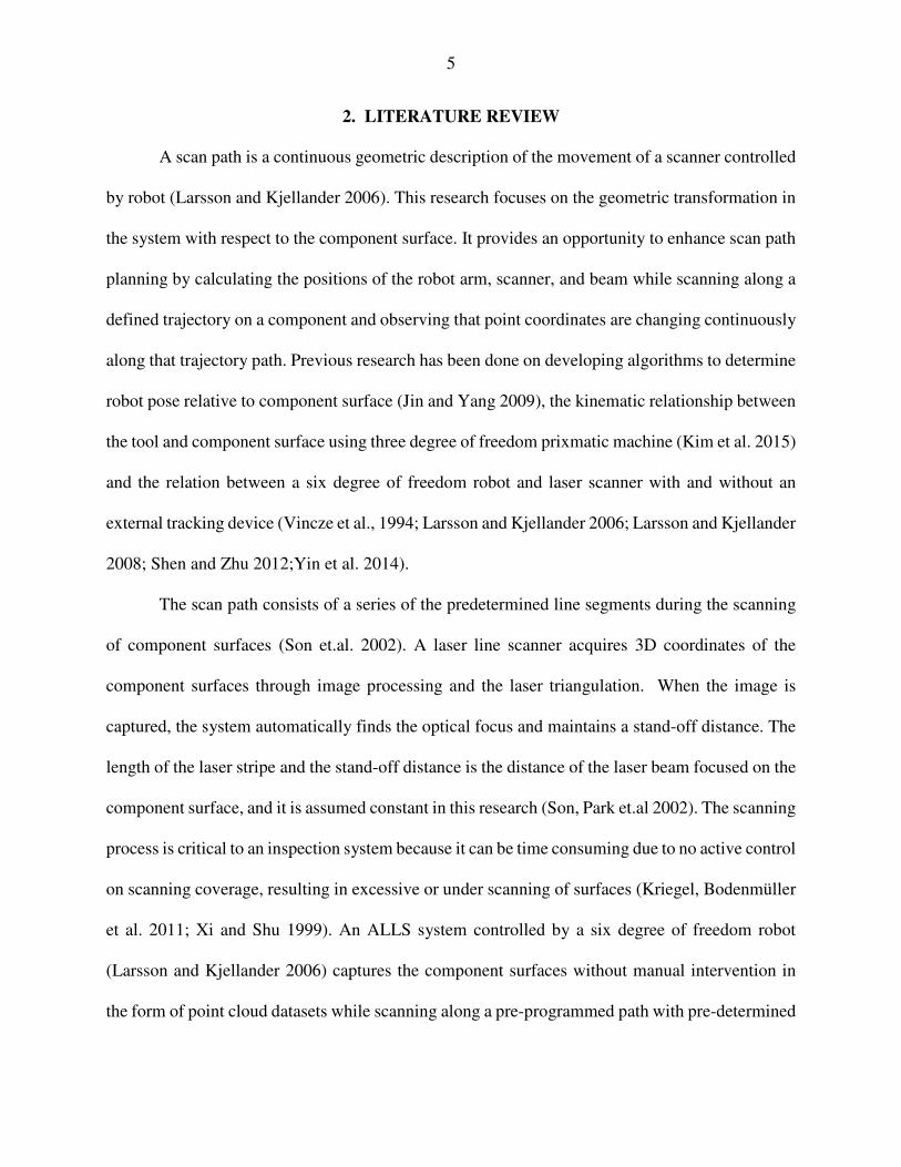
surface data by employing various efficient scanning methods and analyzing point cloud data, the
kinematic relationship between the robot, scanner, and fixed component surface, as shown in
Figure 1, without an external measuring device is to be fully determined.
3
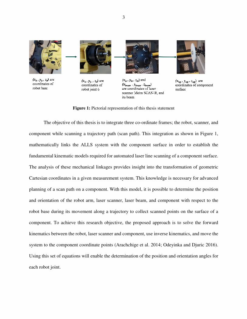
Figure 1: Pictorial representation of this thesis statement
The objective of this thesis is to integrate three co-ordinate frames; the robot, scanner, and
component while scanning a trajectory path (scan path). This integration as shown in Figure 1,
mathematically links the ALLS system with the component surface in order to establish the
fundamental kinematic models required for automated laser line scanning of a component surface.
The analysis of these mechanical linkages provides insight into the transformation of geometric
Cartesian coordinates in a given measurement system. This knowledge is necessary for advanced
planning of a scan path on a component. With this model, it is possible to determine the position
and orientation of the robot arm, laser scanner, laser beam, and component with respect to the
robot base during its movement along a trajectory to collect scanned points on the surface of a
component. To achieve this research objective, the proposed approach is to solve the forward
kinematics between the robot, laser scanner and component, use inverse kinematics, and move the
system to the component coordinate points (Arachchige et al. 2014; Odeyinka and Djuric 2016).
Using this set of equations will enable the determination of the position and orientation angles for
each robot joint.

4
The remainder of this thesis is organized in the following manner: chapter 2 explains the
literature review, chapter 3 describes the elements of an ALLS system, chapter 4 explores the
modelling approach of the ALLS system, chapter 5 states the validation results of the model,
chapter 6 mentions about the scanning experiment to obtain trajectory scan path, and the last
chapter 7 describes conclusions drawn from the generated model as well as the future scope of this
work.
5
2. LITERATURE REVIEW
A scan path is a continuous geometric description of the movement of a scanner controlled
by robot (Larsson and Kjellander 2006). This research focuses on the geometric transformation in
the system with respect to the component surface. It provides an opportunity to enhance scan path
planning by calculating the positions of the robot arm, scanner, and beam while scanning along a
defined trajectory on a component and observing that point coordinates are changing continuously
along that trajectory path. Previous research has been done on developing algorithms to determine
robot pose relative to component surface (Jin and Yang 2009), the kinematic relationship between
the tool and component surface using three degree of freedom prixmatic machine (Kim et al. 2015)
and the relation between a six degree of freedom robot and laser scanner with and without an
external tracking device (Vincze et al., 1994; Larsson and Kjellander 2006; Larsson and Kjellander
2008; Shen and Zhu 2012;Yin et al. 2014).
The scan path consists of a series of the predetermined line segments during the scanning
of component surfaces (Son et.al. 2002). A laser line scanner acquires 3D coordinates of the
component surfaces through image processing and the laser triangulation. When the image is
captured, the system automatically finds the optical focus and maintains a stand-off distance. The
length of the laser stripe and the stand-off distance is the distance of the laser beam focused on the
component surface, and it is assumed constant in this research (Son, Park et.al 2002). The scanning
process is critical to an inspection system because it can be time consuming due to no active control
on scanning coverage, resulting in excessive or under scanning of surfaces (Kriegel, Bodenmüller
et al. 2011; Xi and Shu 1999). An ALLS system controlled by a six degree of freedom robot
(Larsson and Kjellander 2006) captures the component surfaces without manual intervention in
the form of point cloud datasets while scanning along a pre-programmed path with pre-determined
6
scan parameters. These scan parameters are selected based on the component surface and
inspection objectives. An ALLS system research has focused on problems of data capturing
(Larsson and Kjellander 2006), scan path planning strategies (Larsson and Kjellander 2008), and
analysis of point cloud datasets (Pauly et al. 2004; Lu and Milios 1997; Beringia et al. 2009) but
focus on the scan points on the component surface corresponds to the position and orientation of
the robot-scanning system is less explored. Hence, it has turned the attention of researchers to
determine the kinematic relationship between the robot frame and the laser frame.
2.1 Data capturing problem
An automatic scanning system captures the “as- is” data of the part surface, and the
scanning result is a point cloud, which is in a triangular mesh or point form (Surmann, Nüchter et
al. 2003; Stamos and Leordean 2003). The quality of this ‘as-is’ point cloud data depends on the
maximum number of points collected while scanning the path. Component surface data is captured
by planning a scan path along a component surface. In Larsson & Kjellander (2006) ALLS system,
a laser scanner is mounted on a robot in combination with a turntable, and it is moved along a scan
path. Consequently, it becomes important to know the relation between the robot poses in relation
to the component surface. The robot poses are defined as the robot-scanner moves to view the
object from different positions while the scanner scans the component surface. The component
surface is rotated using a turntable (Larsson and Kjellander 2006), and a robot moves the scanner
to view the surface from different angles using camera. Hence, during data capturing it is necessary
to know the rotation angle of the turntable with respect to the robot position in order to move the
robot.
7
2.2 Scan path planning strategies
The focus of previous work regarding scan path planning has included different scan path
planning strategies, an algorithm to generate a scan path using the CAD model (Jin and Yang
2009), laser line scanner parameters that affect the scan path (ElMaraghy and Yang 2003), and a
path or view planning method to orient the measuring system relative to the object in each
individual scan (Larsson and Kjellander 2008). Different scan path planning strategies intending
to improve the quality of scan data are done by: (i) interpreting geometrical data measured directly
from surface of existing objects, (ii) breaking broken regions into layers of worn out parts (Wu
and Hu 2012), (iii) direct slicing to obtain path data on curved surface (Xi and Shu 1999; Bračun
et al. 2006; Mehdi-Souzani, Thiébaut et al. 2006; Fernández, Rico et al. 2008; Jin and Yang 2009;
Larsson and Kjellander 2008), and on existing objects with predefined scan patterns (ElMaraghy
and Yang 2003). To implement different scan path planning methodologies with an ALLS system,
we need to first understand the transformation in geometric coordinates during scanning given a
component surface.
2.3 Analysis of point cloud datasets
Point cloud datasets are obtained from a scanned component surface (Derigent, Chapotot
et al. 2007; Durupt, Remy et al. 2008). Due to cumbersome scanning procedures, problems of
inconsistencies, uncertainty, and variations are observed in point cloud data. There are different
methods to solve the uncertainty and variation in a point cloud by analyzing these datasets in
various forms to extract high level information about scanned objects and to create renditions
meaningful to a user by modifying the shape or appearance of point cloud data (Pauly et al. 2004).
A study by Lu and Milios (1997) attempted to solve the problem of inconsistency in point cloud
datasets by collecting and estimating two scans from two different robot poses. While scanning is
8
done, the two scans are aligned and matched (Borangiu et al. 2009). An alternative approach
addressed in this thesis is to focus on understanding the fundamental changes in the kinematic
structure of an automated laser scanning system based on its relative position and orientation while
moving on the trajectory of a component surface. The quality of the point cloud depends on the
closeness to measured points along a scan path. This collection of closely measured points on a
scan path has gathered importance in manufacturing, reverse engineering and remanufacturing due
to growing interest in advanced inspection systems, the model based enterprise and the product or
manufacturing digital thread (Rickli.et.al. 2014). This shifts the focus from analyzing point cloud
segments (Triebel et al. 2004) to studying the occurrence of the geometric transformation of point
coordinates while scanning surfaces or moving along a trajectory.
2.4 Paradigm shift
There has been little focus on the geometric movement of the ALLS system transformation
of the coordinates from one aspect of the system to another. This provides an opportunity to
enhance the scan path calculations of various positions of a robot arm, scanner, and beam while
scanning along a defined trajectory on a component and making the observation that point
coordinates are changing continuously along that trajectory. Although a few researchers (Shen
and Zhu 2012;Yin et al. 2014) have worked to determine the kinematic relation of fixed frames
and moving frames like a robot and laser line scanner (Yin et al. 2014), as well as the relation
between tool and the component systems with respect to a three degree of freedom machine (Kim
et al. 2015), there has been little research focused on the integration of all three elements (robot,
scanner, and component surface) to determine the geometric coordinate changes along a trajectory
path of a component surface. This gap leads to a paradigm shift on the approach of solving the
problem of obtaining better point cloud data by integrating the ALLS system and component
9
surface coordinate systems. The determination of such a relation provokes the need to understand
the geometric transformation of coordinates during the scanning movement of the ALLS system.
Thus, it is critical to determine the changing kinematic structure during the movement of the entire
ALLS system while moving across a trajectory for a given component to fully understand the
kinematic mechanism occurring during point cloud measurements (Buchsbaum and Freudenstein
1970).
The system’s mechanical linkages move along a fixed trajectory on the surface of a
component, which changes the position and orientation of coordinates of the three elements of
system. This movement is fixed at the robot base, while other joints up to the laser beam move as
one mechanical linkage along a trajectory. As a result, the orientation transformation matrix of the
end effector, laser scanner, and laser beam joints can be obtained. The coordinates of the points on
the trajectory of a component are calculated by solving the geometrical equations of the shape of
the component surface, assuming the component is fixed with respect to the robot’s base. However,
to move all the mechanical linkages to this fixed point on the component, the joint angles of robot
(θ1-, θ6) , laser line scanner (θls), and laser beam (θbeam) must be determined by using inverse
kinematic equations for six degree FANUC S430 IW robot (Odeyinka and Djuric 2016). Thus, we
can understand the geometrical transformation from one coordinate system transform to another
coordinate while moving the system along a scan path. This helps to determine the position
coordinates for the end effector, laser scanner, and beam to move on a trajectory point on the
surface of the component.
2.2 Related kinematic models
Several researchers (Vincze, Prenninger et al. 1994; Leigh-Lancaster, Shirinzadeh et al.
1997; Feng, Liu et al. 2001; Santolaria, Guillomía et al. 2009; Wang, Mastrogiacomo et al. 2011;
10
Paoli and Razionale 2012; Norman, Schönberg et al. 2013) have targeted the kinematic relation
between a robot and a laser line scanner using an external laser tracking system. The kinematic
relation between the robot and laser scanner without an external tracker using a linear rail type of
a moving linkage to support a stationary laser scanner (Yin et al. 2014) and the relation between
three degree of freedom machine, tool, and component system with respect to an arbitrary
component surface (Kim et al. 2015) are extended in this work by determining the kinematic
relationship for a six degree of freedom robot, scanner, and spherical component surface during
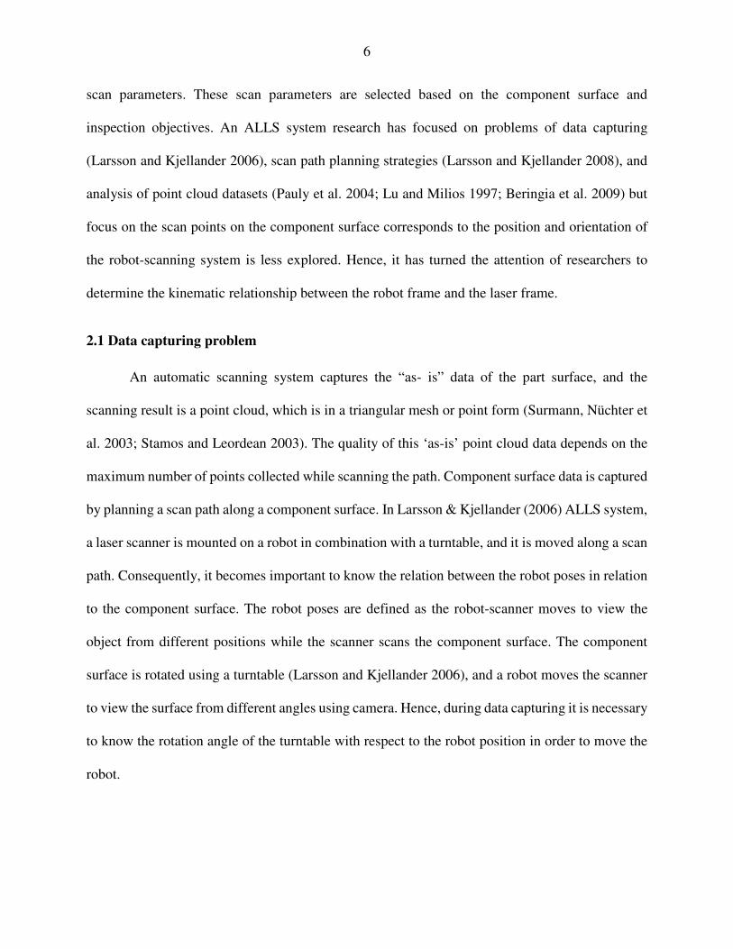
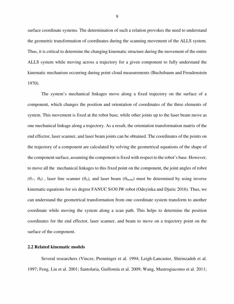
the scanning motion. The position and orientation coordinates for each element of the system
determine the position and orientation of the robot end effector Oe (xe, ye, ze) and laser scanner Os
(xs, ys, zs) while the robot is in arbitrary motion, as shown in Figure 2. The geometric transform
relationship between the robot end effector frame and the laser scanner without an external tracker
is called the hand-eye calibration of a laser probe and robot (Dornaika and Horaud 1998; Yin et
al. 2014).
Figure 2: Integrated 3D scanning system (Yin, Ren et al. 2014)
As shown in Figure 2, a fixed scanner and sensor are mounted on a moving scanning frame
as a rail frame. The end effector (EF) of robot has coordinates Oe (xe, ye, ze), scanning frame (SF)
11
Os (xs, ys, zs), and linear frame (LF) has coordinates Ol (xl, yl, zl) with respect to the robot base
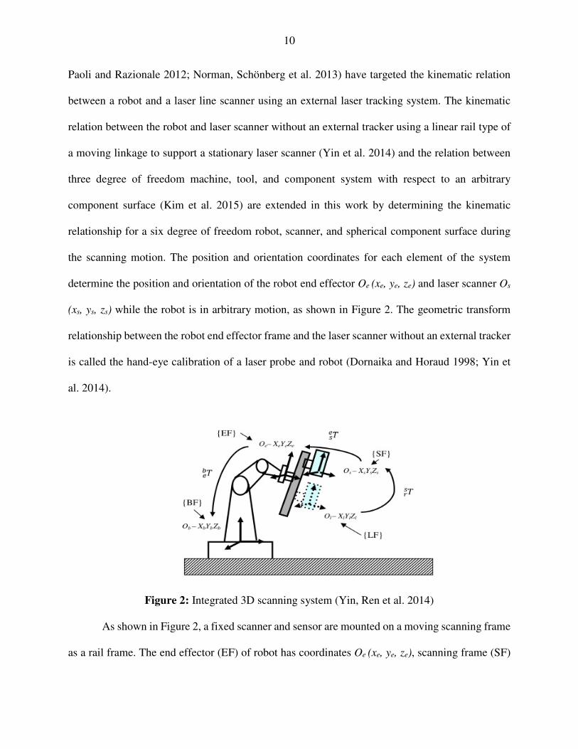
coordinates Os (xb, yb, zb). The shape and position information of local features within the range of
the rail frame are obtained by multiplying 4x4 homogenous matrices as described in Yin et al.
(2014), Eq. 1 derives the relationship between the coordinate, Pb, in the robot base frame and Pl
in the laser sensor frame.
= ∗ ∗ ∗ Eq. (1)
Where , and are 4x4 homogenous coordinate transform matrices. is the
transform relationship between the laser sensor and the rail scanning frame, is transformation
between the rail scanning frame and robot end effector frame, denotes transform relationship
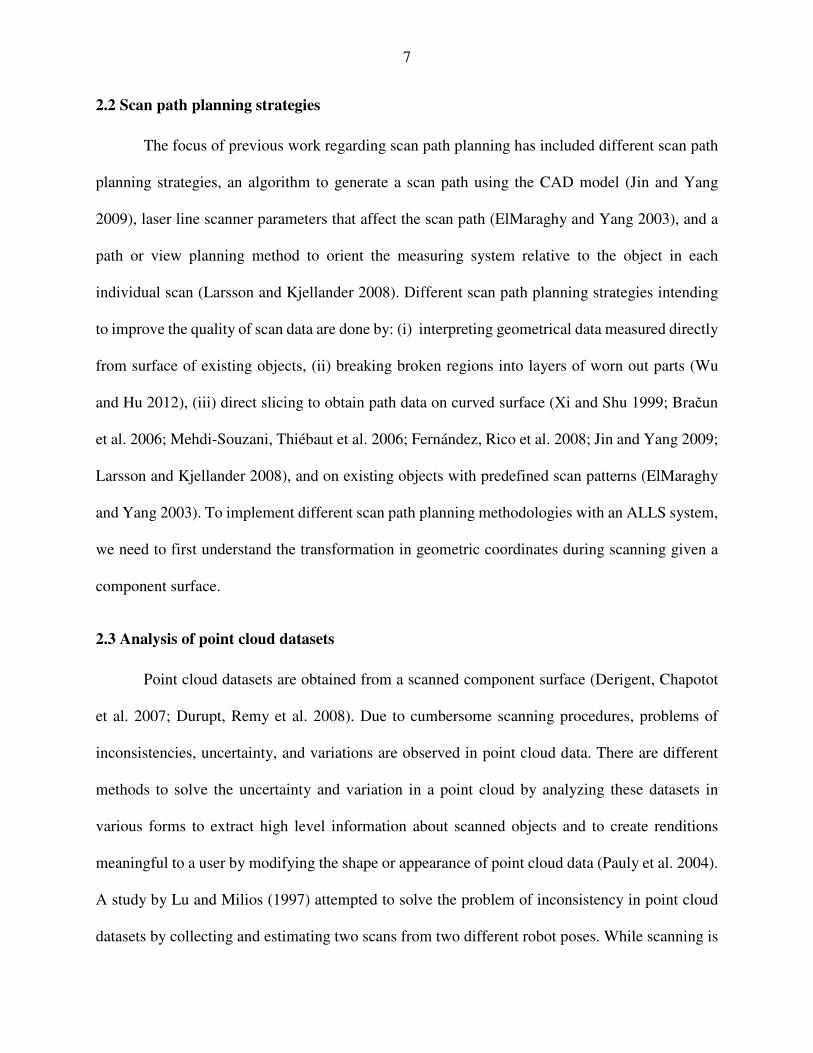
between the robot end effector and the robot base. The model in Figure 3 (Yin et al. 2014)
formulates the relationship between the spheres centers measured for different robot poses with
the laser sensor frame changes. These models provide insight into formulating the relationship
between different coordinate frames of each element of this ALLS system.
Figure 3: Relationship between the scanning frame and robot frame (Yin et al. 2014)
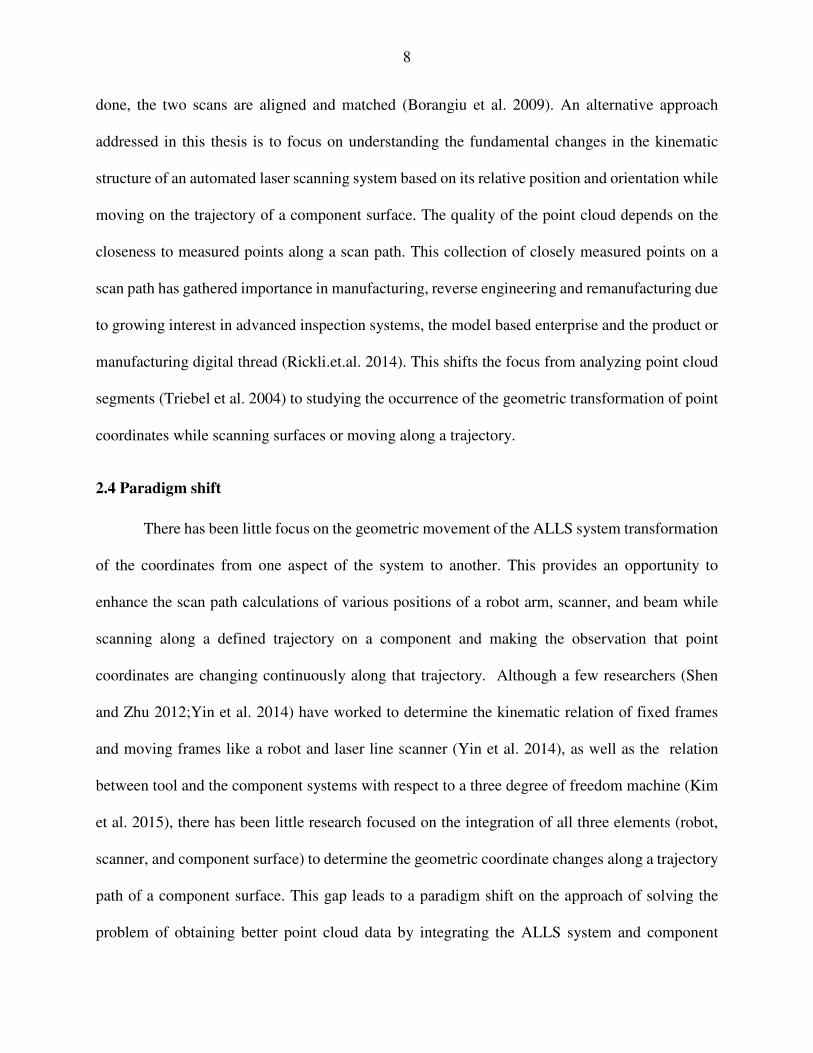
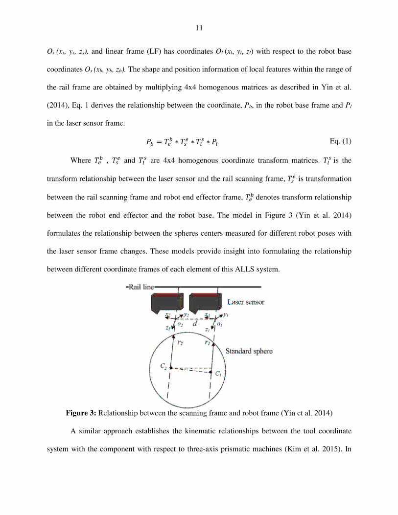
A similar approach establishes the kinematic relationships between the tool coordinate
system with the component with respect to three-axis prismatic machines (Kim et al. 2015). In
12
their work as shown in Figure 4, the tool frame (xt, yt, zt) is perpendicular to the arbitrary
component surface (xa, ya, za). The steps to plan the trajectory are as follows: derive the surface
tangent vectors of the curved surface in the component local coordinate system, determine the
forward kinematics from the local coordinate and the tool coordinate, and calculate the joint
parameters using inverse kinematics. While this application is not targeted for laser line scanners,
it contributes towards developing the approach for the orientation of the laser scanner
perpendicular to the component in order to determine the kinematic relationship between a laser
line scanner and component coordinates with respect to the robot base (xb, yb, zb).
Figure 4: Kinematics of robot-base, tool, and surface for a wire embedding process (Kim et al. s
2015).
This research fills the research gap to undertake the study of geometric coordinates in
automated laser scanning system elements relative to component surface. The summary of
literature review is presented in the Table 1, which provides the gap of this research and helps to
understand this thesis contribution. The distinguishing elements of the ALLS system in our
research are the six degree of freedom robot, laser scanner, and stationary component instead of a
three degree of freedom robot and tool (Kim et al. 2015), or a rail scanning frame to support the
stationary laser scanner, laser sensor, and component mounted on a turntable (Yin et al. 2014).
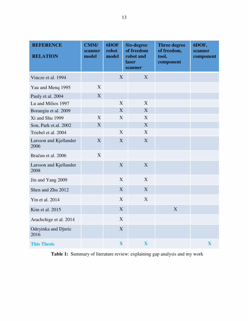
13
REFERENCE
RELATION
CMM/
scanner
model
6DOF
robot
model
Six-degree
of freedom
robot and
laser
scanner
Three degree
of freedom,
tool,
component
6DOF, scanner
component
Vincze et al. 1994 X X
Yau and Menq 1995 X
Pauly et al. 2004 X
Lu and Milios 1997 X X
Borangiu et al. 2009 X X
Xi and Shu 1999 X X X
Son, Park et.al. 2002 X X
Triebel et al. 2004 X X
Larsson and Kjellander 2006
X X X
Bračun et al. 2006 X
Larsson and Kjellander 2008
X X
Jin and Yang 2009 X X
Shen and Zhu 2012 X X
Yin et al. 2014 X X
Kim et al. 2015 X X
Arachchige et al. 2014 X
Odeyinka and Djuric 2016
X
This Thesis X X X
Table 1: Summary of literature review: explaining gap analysis and my work

14
3. ELEMENTS OF ALLS SYSTEM
The ALLS system is an inspection scanning system consists of laser line scanner attached
as tool frame to the six degree of freedom FANUC S-430 IW robot. During scanning motion, as
this inspection system is moved, the changes in geometry of the system changes. The kinematics
of the laser line scanner and the FANUC S-430 IW robot are explained in detail in this chapter.
3.1 Laser Line scanner- MetraSCAN-R scanner
Laser line scanner measurement operates by the controlled deflection and steering of laser
beams, followed by a distance measurement at every pointing direction. A 3D laser scanner
consists of a laser, ranging unit, and control data unit. The laser unit is a deflecting or rotating unit
that produces the laser beam or pulse that is needed for measurement. The ranging unit is a signal
processing unit in which distances and angles are determined. To develop an ALLS system the
triangulation of 3D laser scanners must be known. A laser stripe projects onto the component
surface, and the reflected beam is detected by cameras. Through this method, the three dimensional
coordinates are acquired. The laser line is a function of the view angle limit, the location vector of
the source, the stand-off distance, and a vector perpendicular to the laser source (Son et al. 2002).
The laser projector and sensor are modeled as the coordinate systems of the laser projector, the
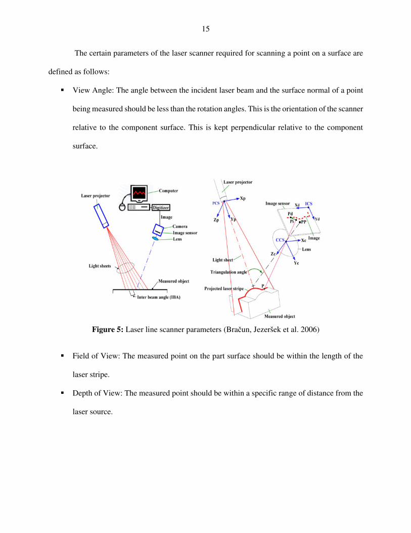
lens, the sensor, and the component surface (Bračun et al. 2006). A scanning system automatically
finds an optical focus and maintains a certain distance, called a stand-off distance, between the end
of the laser probe and the beam focused on the component; refer to Figure 5 (Bračun et al. 2006).
The incident beam and reflected beam should not interfere with the part itself. The laser scanner
should be kept at a collision free distance from the component surface.
15
The certain parameters of the laser scanner required for scanning a point on a surface are
defined as follows:
View Angle: The angle between the incident laser beam and the surface normal of a point
being measured should be less than the rotation angles. This is the orientation of the scanner
relative to the component surface. This is kept perpendicular relative to the component
surface.
Figure 5: Laser line scanner parameters (Bračun, Jezeršek et al. 2006)
Field of View: The measured point on the part surface should be within the length of the
laser stripe.
Depth of View: The measured point should be within a specific range of distance from the
laser source.
16
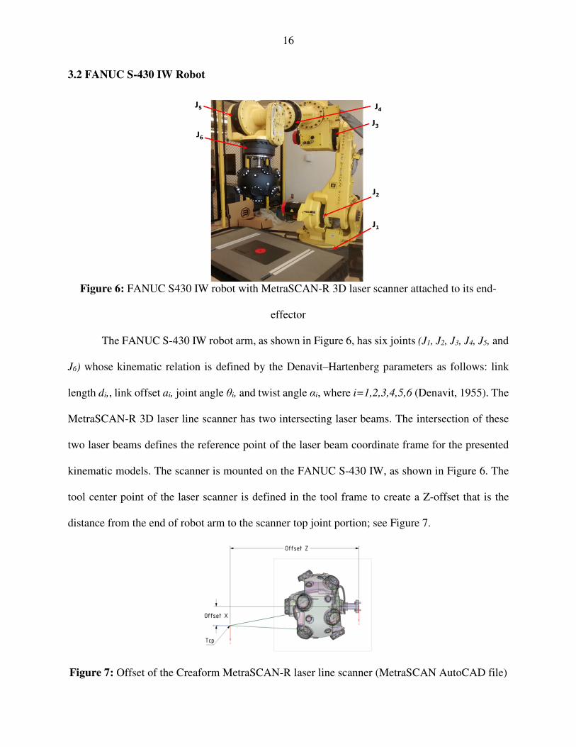
3.2 FANUC S-430 IW Robot
Figure 6: FANUC S430 IW robot with MetraSCAN-R 3D laser scanner attached to its end-
effector
The FANUC S-430 IW robot arm, as shown in Figure 6, has six joints (J1, J2, J3, J4, J5, and
J6) whose kinematic relation is defined by the Denavit–Hartenberg parameters as follows: link
length di,, link offset ai, joint angle θi, and twist angle αi, where i=1,2,3,4,5,6 (Denavit, 1955). The
MetraSCAN-R 3D laser line scanner has two intersecting laser beams. The intersection of these
two laser beams defines the reference point of the laser beam coordinate frame for the presented
kinematic models. The scanner is mounted on the FANUC S-430 IW, as shown in Figure 6. The
tool center point of the laser scanner is defined in the tool frame to create a Z-offset that is the
distance from the end of robot arm to the scanner top joint portion; see Figure 7.
Figure 7: Offset of the Creaform MetraSCAN-R laser line scanner (MetraSCAN AutoCAD file)
17
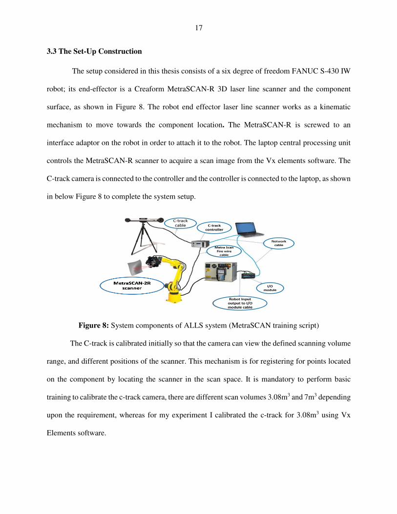
3.3 The Set-Up Construction
The setup considered in this thesis consists of a six degree of freedom FANUC S-430 IW
robot; its end-effector is a Creaform MetraSCAN-R 3D laser line scanner and the component
surface, as shown in Figure 8. The robot end effector laser line scanner works as a kinematic
mechanism to move towards the component location. The MetraSCAN-R is screwed to an
interface adaptor on the robot in order to attach it to the robot. The laptop central processing unit
controls the MetraSCAN-R scanner to acquire a scan image from the Vx elements software. The
C-track camera is connected to the controller and the controller is connected to the laptop, as shown
in below Figure 8 to complete the system setup.
Figure 8: System components of ALLS system (MetraSCAN training script)
The C-track is calibrated initially so that the camera can view the defined scanning volume
range, and different positions of the scanner. This mechanism is for registering for points located
on the component by locating the scanner in the scan space. It is mandatory to perform basic
training to calibrate the c-track camera, there are different scan volumes 3.08m3 and 7m3 depending
upon the requirement, whereas for my experiment I calibrated the c-track for 3.08m3 using Vx
Elements software.

18
4. MODELING OF ALLS SYSTEM
The kinematics modeling is accomplished by following the below steps:
i. Solve the forward kinematics equations for the six degree of freedom robot, the laser
scanner, and the laser beam. This validates the position of the model of the entire
measurement system.
ii. Define the component surface by calculating the equation of the surface and point
coordinates on its surface.
iii. Calculate the joint angles for the robot, scanner, and beam using inverse kinematic
equations and move the robot to the point on the component’s surface to get a trajectory
path for scanning.
4.1 Forward Kinematics, Step (i):
Mechanical linkages of the system are validated by solving forward kinematics by defining
the position coordinates of the robot end effector, scanner, and beam. The validation position for
the FANUC LR 200 IC robot is obtained by Arachchige et.al (2014), but it is extended in this
research by solving the forward kinematic equations to obtain the validated position for the
FANUC S-430 IW robot, laser scanner, and laser beam. The kinematic structure of the FANUC
S-430 IW, MetraSCAN-R scanner, and beam are shown in Figure 9. The relationship between the
two links of the joints can be described using Denavit and Hartenberg (1955) parameters
represented as follows: link lengths (d1-d6 ) (Kashani et.al. 2010), link offset (a1-a6), joint angles
(θ1-θ6), and twist angle (α1-α6) for the robot. The scanner is added as the tool frame, where als is
the width of laser scanner, abeam is the width of the beam from its cross-section, dls is the length of
the scanner, dbeam is the length of the laser stripe and stand-off distance, αls is the twist angle of the
laser scanner, αbeam is the twist angle of the laser beam, θls is the joint angle of the laser scanner,
19
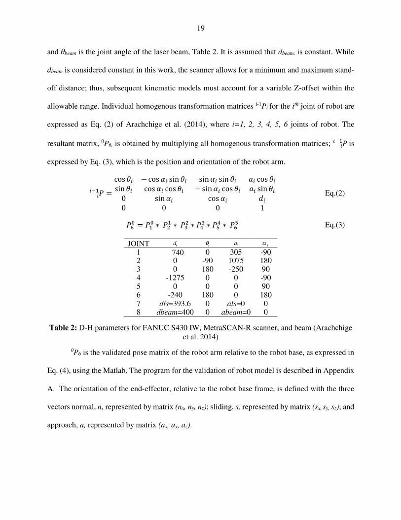
and θbeam is the joint angle of the laser beam, Table 2. It is assumed that dbeam, is constant. While
dbeam is considered constant in this work, the scanner allows for a minimum and maximum stand-
off distance; thus, subsequent kinematic models must account for a variable Z-offset within the
allowable range. Individual homogenous transformation matrices i-1Pi for the ith joint of robot are
expressed as Eq. (2) of Arachchige et al. (2014), where i=1, 2, 3, 4, 5, 6 joints of robot. The
resultant matrix, 0P6, is obtained by multiplying all homogenous transformation matrices; is
expressed by Eq. (3), which is the position and orientation of the robot arm.
= cos − cos sin sin sin cos sin cos cos − sin cos sin 0 sin cos 0 0 0 1 Eq.(2)
= ∗ ∗ ∗ ∗ ∗ Eq.(3)
JOINT id iθ ia iα 1 740 0 305 -90 2 0 -90 1075 180 3 0 180 -250 90 4 -1275 0 0 -90 5 0 0 0 90 6 -240 180 0 180 7 dls=393.6 0 als=0 0 8 dbeam=400 0 abeam=0 0
Table 2: D-H parameters for FANUC S430 IW, MetraSCAN-R scanner, and beam (Arachchige et al. 2014)
0P6 is the validated pose matrix of the robot arm relative to the robot base, as expressed in
Eq. (4), using the Matlab. The program for the validation of robot model is described in Appendix
A. The orientation of the end-effector, relative to the robot base frame, is defined with the three
vectors normal, n, represented by matrix (nx, ny, nz); sliding, s, represented by matrix (sx, sy, sz); and
approach, a, represented by matrix (ax, ay, az).
20
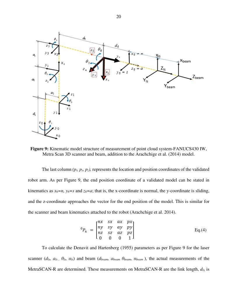
Figure 9: Kinematic model structure of measurement of point cloud system-FANUCS430 IW,
Metra Scan 3D scanner and beam, addition to the Arachchige et al. (2014) model.
The last column (px, py, pz), represents the location and position coordinates of the validated
robot arm. As per Figure 9, the end position coordinate of a validated model can be stated in
kinematics as x6=n, y6=s and z6=a; that is, the x-coordinate is normal, the y-coordinate is sliding,
and the z-coordinate approaches the vector for the end position of the model. This is similar for
the scanner and beam kinematics attached to the robot (Arachchige et al. 2014).
= !" #" " $"!% #% % $%!& #& & $&0 0 0 1 ' Eq.(4)
To calculate the Denavit and Hartenberg (1955) parameters as per Figure 9 for the laser
scanner (dls, als , θls, αls) and beam (dbeam, abeam θbeam, αbeam ), the actual measurements of the
MetraSCAN-R are determined. These measurements on MetraSCAN-R are the link length, dls, is
21
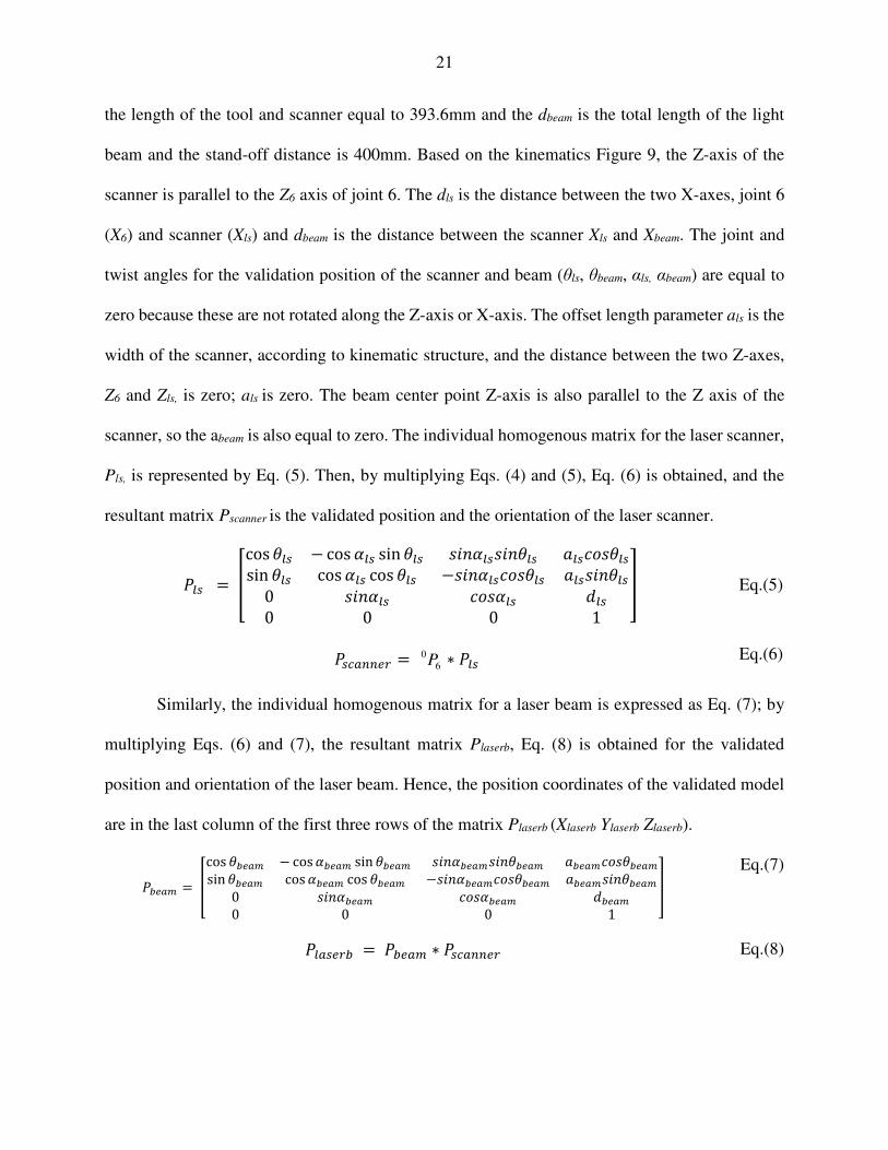
the length of the tool and scanner equal to 393.6mm and the dbeam is the total length of the light
beam and the stand-off distance is 400mm. Based on the kinematics Figure 9, the Z-axis of the
scanner is parallel to the Z6 axis of joint 6. The dls is the distance between the two X-axes, joint 6
(X6) and scanner (Xls) and dbeam is the distance between the scanner Xls and Xbeam. The joint and
twist angles for the validation position of the scanner and beam (θls, θbeam, αls, αbeam) are equal to
zero because these are not rotated along the Z-axis or X-axis. The offset length parameter als is the
width of the scanner, according to kinematic structure, and the distance between the two Z-axes,
Z6 and Zls, is zero; als is zero. The beam center point Z-axis is also parallel to the Z axis of the
scanner, so the abeam is also equal to zero. The individual homogenous matrix for the laser scanner,
Pls, is represented by Eq. (5). Then, by multiplying Eqs. (4) and (5), Eq. (6) is obtained, and the
resultant matrix Pscanner is the validated position and the orientation of the laser scanner.
= (cos − cos sin #)!#)! *+#sin cos cos −#)!*+# #)!0 #)! *+# 0 0 0 1 , Eq.(5)
-.//0 = 60P ∗ Eq.(6)
Similarly, the individual homogenous matrix for a laser beam is expressed as Eq. (7); by
multiplying Eqs. (6) and (7), the resultant matrix Plaserb, Eq. (8) is obtained for the validated
position and orientation of the laser beam. Hence, the position coordinates of the validated model
are in the last column of the first three rows of the matrix Plaserb (Xlaserb Ylaserb Zlaserb).
.1 = (cos .1 − cos .1 sin .1 #)!.1#)!.1 .1*+#.1sin .1 cos .1 cos .1 −#)!.1*+#.1 .1#)!.10 #)!.1 *+#.1 .10 0 0 1 , Eq.(7)
.0 = .1 ∗ -.//0 Eq.(8)
22
4.2 Component surface, Step (ii):
The assumption of our model to transform the relationship from the laser scanner frame to
the component surface frame states that the component is a sphere. The approach can be applied
to other component surfaces by replacing this surface representation. More complex surfaces may
require integration with CAD model data. The spherical coordinate system is used for specifying
the position of the point on the surface (Fu et.al. 1987), which involves the following translations
or rotations: translation of the radius, r, in the Z-axis direction; rotation, α, about the Z-axis; and
rotation, β, about the x-axis. The Matlab program for deriving the equation of component surface
is described in Appendix B.
4.3 Inverse Kinematics, Step (iii):
Inverse kinematics is the approach for general serial manipulators to compute joint
displacements for a given pose of the end effector (Manocha & Canny, 1994). This inverse
kinematics solution is required to calculate the joint angles (θ1 to θ6) for six degree of freedom
FANUC S-430 IW (Odeyinka. 2015; Odeyinka and Djuric 2016). In this research these inverse
kinematic equations are modified slightly to validate the FANUC S-430 IW robot along with the
laser scanner end-effector. The modelling of the scanner and the beam has been done by adding
two frames as an offset; as a result, Eq. (9) is implemented in the inverse kinematics solutions to
determine the joint angles of the robot (θ1 to θ6). To solve this approach the first step is to find the
first three joints and then the last three joints (Pieper 1968). In the calculation of the first three
joint angles the first step is to locate the intersection of the last three joints axes and calculate the
position of this intersection point, from the desired position vector p and pose R of the end effector.
In Figure 10, the vector p is projected onto the x0-y0 plane at joint 1 of FANUC S430 IW, the link
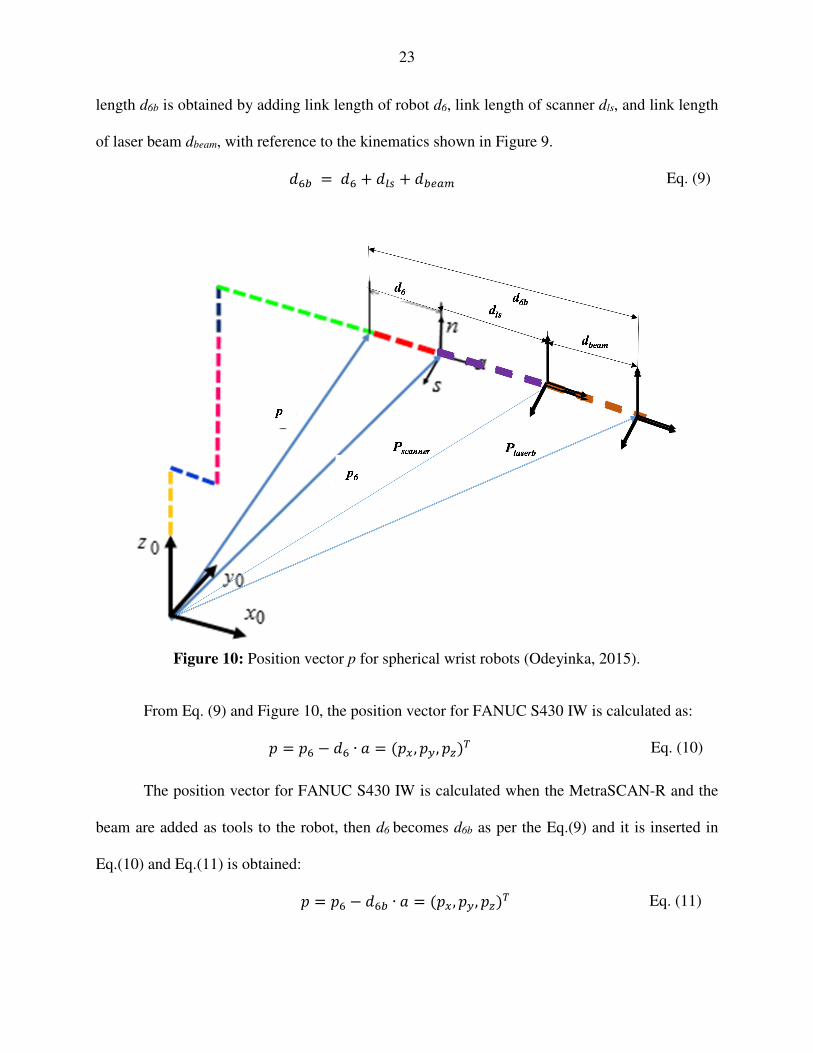
23
length d6b is obtained by adding link length of robot d6, link length of scanner dls, and link length
of laser beam dbeam, with reference to the kinematics shown in Figure 9.
2 2 .1 Eq. (9)
Figure 10: Position vector p for spherical wrist robots (Odeyinka, 2015).
From Eq. (9) and Figure 10, the position vector for FANUC S430 IW is calculated as:
$ $ ∙ 4$5, $6 , $789 Eq. (10)
The position vector for FANUC S430 IW is calculated when the MetraSCAN-R and the
beam are added as tools to the robot, then d6 becomes d6b as per the Eq.(9) and it is inserted in
Eq.(10) and Eq.(11) is obtained:
$ $ ∙ 4$5, $6 , $789 Eq. (11)
24
Hence, according to Eqn. (11) each coordinate of p (px, py, pz) is calculated from Eq. (10) is
mentioned in Eq. (12) as:
$" $5 :#48 ∙ 5
$% $6 :#48 ∙ 6
$& $7 :#48 ∙ 7
Eq. (12)
Whereas, Px6, Py6, and Pz6 in Eq. (12) are the position vector of 0P6 the values of last column
of matrix and ax, ay, and az are the approach vector of P6, the values of third column of matrix
obtained from Eq. (4).
4.3.1 Joint 1 solution:
The joint 1 solution for FANUC S-430IW is obtained by projecting the position vector p
onto x0-y0. The position vector p, points from the origin of the shoulder coordinate system to the
point where the last three joints axis are intersecting. The last three joint axes intersect at point D.
This point is the Wrist Center Point (WCP) as shown in Figure 11. Motion of the final three joints
about these axes will not change the position of D. Position of the wrist center is a function of only
the first three joint angles (Odeyinka and Djuric 2016). The ARM, ELBOW and WRIST
definitions for FANUC robot family are discussed (Odeyinka and Djuric 2016):
I. Left Arm (LA): when positive θ2 moves the wrist in negative direction while θ3 is not active
II. Right Arm (RA): when positive θ2 moves wrist positive z0 direction while θ3 is not active.
III. Above Arm or Elbow above wrist: when the position of the wrist to the RA/LA with respect
to the shoulder coordinate system has negative/positive coordinate value along the y2 axis.
IV. Below Arm (BA) or Elbow Below wrist: When the position of the wrist to the RA/LA with
respect to the shoulder coordinate system has positive/negative coordinate value along the
y2 axis.
25
V. Wrist Down (WD): when the s unit vector of the hand coordinate system and the y5 unit
vector of the coordinate system (xs, ys, zs ) have a positive dot product, i.e. # ∙ %5 < 0 VI. Wrist Up (WU): when the s unit vector of the hand coordinate system and the y5 unit vector
of the coordinate system (xs, ys, zs ) have a negative dot product, i.e. # ∙ %5 < 0
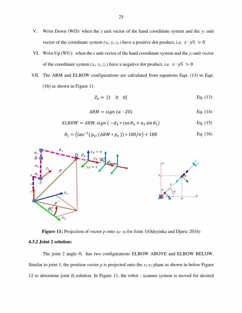
VII. The ARM and ELBOW configurations are calculated from equations Eqn. (13) to Eqn.
(16) as shown in Figure 11.
= >1 0 0? Eq. (13)
@AB #)C!4 ∙ =08 Eq. (14)
DEFGH @AB. #)C!4 ∗ cos 2 sin 8 Eq. (15)
Jtan 4 $6 , 4@AB ∗ $588 ∗ 180/OP 2 180 Eq. (16)
Figure 11: Projection of vector p onto x0- y0 for Joint 1(Odeyinka and Djuric 2016)
4.3.2 Joint 2 solution:
The joint 2 angle θ2 has two configurations ELBOW ABOVE and ELBOW BELOW.
Similar to joint 1, the position vector p is projected onto the x1-y1 plane as shown in below Figure
12 to determine joint θ2 solution. In Figure 11, the robot - scanner system is moved for desired
26
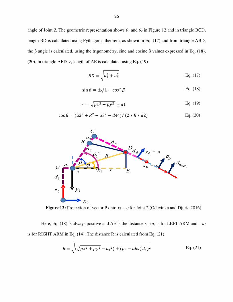
angle of Joint 2. The geometric representation shows θ1 and θ2 in Figure 12 and in triangle BCD,
length BD is calculated using Pythagoras theorem, as shown in Eq. (17) and from triangle ABD,
the β angle is calculated, using the trigonometry, sine and cosine β values expressed in Eq. (18),
(20). In triangle AED, r, length of AE is calculated using Eq. (19)
FQ R 2 Eq. (17)
sin S TU1 *+# S Eq. (18)
V U$" 2 $% T 1 Eq. (19)
cos S 42 2 A 3 48/42 ∗ A ∗ 28 Eq. (20)
Figure 12: Projection of vector P onto x1 – y1 for Joint 2 (Odeyinka and Djuric 2016)
Here, Eq. (18) is always positive and AE is the distance r, +a1 is for LEFT ARM and – a1
is for RIGHT ARM in Eq. (14). The distance R is calculated from Eq. (21)
A R4U$" 2 $% 8 2 4$& :#4 8 Eq. (21)
27
From Triangle AED of Figure 12, the distance DE is given by Eq. (22) and sine, cosine
values of ∅ is given by Eq. (23) and (24). To calculate θ2 is the inverse tan ratio, using trigonometry
is obtained by Eq. (27) by calculating the sine, cosine values of θ2 is given by Eq. (25) and (26)
QD $7 Eq. (22)
sin ∅ = ( $7 − :#( ))A Eq. (23)
cos ∅ = −VA . @AB Eq. (24)
sin = sin ∅ ∗ cos S + @AB. DEFGH. cos ∅. sin S Eq. (25)
cos = cos ∅ ∗ cos S + @AB. DEFGH. sin ∅. sin S Eq. (26)
= tan sin cos Eq. (27)
Further the ELBOW configuration is defined as the position of the wrist with respect to the
shoulder coordinate system, which has negative or positive coordinate value along the y2-axis, and
this is the Above Arm or Elbow Above wrist. The position of the wrist to the RIGHT/LEFT Arm
with respect to the shoulder coordinate system has a positive or negative coordinate value along
y2 axis. The decision equation is defined by 2P4 in Eq. (28) and the ARM indicator from Eq. (14).
The sign of the decision equation for the ELBOW indicator Eq. (28) is based on the sign of y-
component of the position vector of 3P2 , 4P3, and ARM indicator. There are different values for
joint 3 as shown in Table 3.
= .
% = (1, 2)
DEFGH = @AB ∗ #)C!( % )
Eq. (28)
28
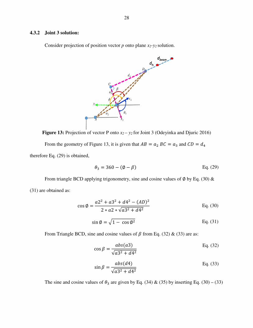
4.3.2 Joint 3 solution:
Consider projection of position vector p onto plane x2-y2 solution.
Figure 13: Projection of vector P onto x2 – y2 for Joint 3 (Odeyinka and Djuric 2016)
From the geometry of Figure 13, it is given that @F F[ and [Q therefore Eq. (29) is obtained,
360 4∅ S8 Eq. (29)
From triangle BCD applying trigonometry, sine and cosine values of ∅ by Eq. (30) &
(31) are obtained as:
cos ∅ 2 2 3 2 4 4@Q82 ∗ 2 ∗ √3 2 4 Eq. (30)
sin ∅ U1 cos ∅ Eq. (31)
From Triangle BCD, sine and cosine values of S from Eq. (32) & (33) are as:
cos S :#438√3 2 4
Eq. (32)
sin S :#448√3 2 4
Eq. (33)
The sine and cosine values of are given by Eq. (34) & (35) by inserting Eq. (30) – (33)
29
sin 3 cos ∅∗ sin S sin ∅ cos S Eq. (34)
cos 3 cos ∅∗ cos S 2 sin ∅. sin S Eq. (35)
3 tan sin 3cos 3 Eq. (36)
Arm Configuration ( )yP42
3θ ARM ELBOW ARM
ELBOW
LEFT and ABOVE 0≥ βα− -1 +1 -1
LEFT and BELOW 0≤ βα− -1 -1 +1
RIGHT and ABOVE 0≤ βα− +1 +1 +1
RIGHT and ABOVE 0≥ βα− +1 -1 -1
Table 3: Different possible arm configurations for joint three (Odeyinka and Djuric 2016)
4.3.4 Joint 4 Solution:
To determine the joint angle θ4 solution, we have to find H, which is the transformation
matrix obtained, Eq. (37), is by multiplication of first three matrices with respect to the base frame
^ = ∗ ∗
Eq. (37) ^ = _` a = b0 0 0 1 c Hence, each matrix X3 Y3, Z3 and F3 can be defined as:
` = ^(1, 1)^(2,1)^(3,1)' a = ^(1, 2)^(2,2)^(3,2)' = = ^(1, 3)^(2,3)^(3,3)' b = ^(1, 4)^(2,4)^(3,4)' Eq. (38)
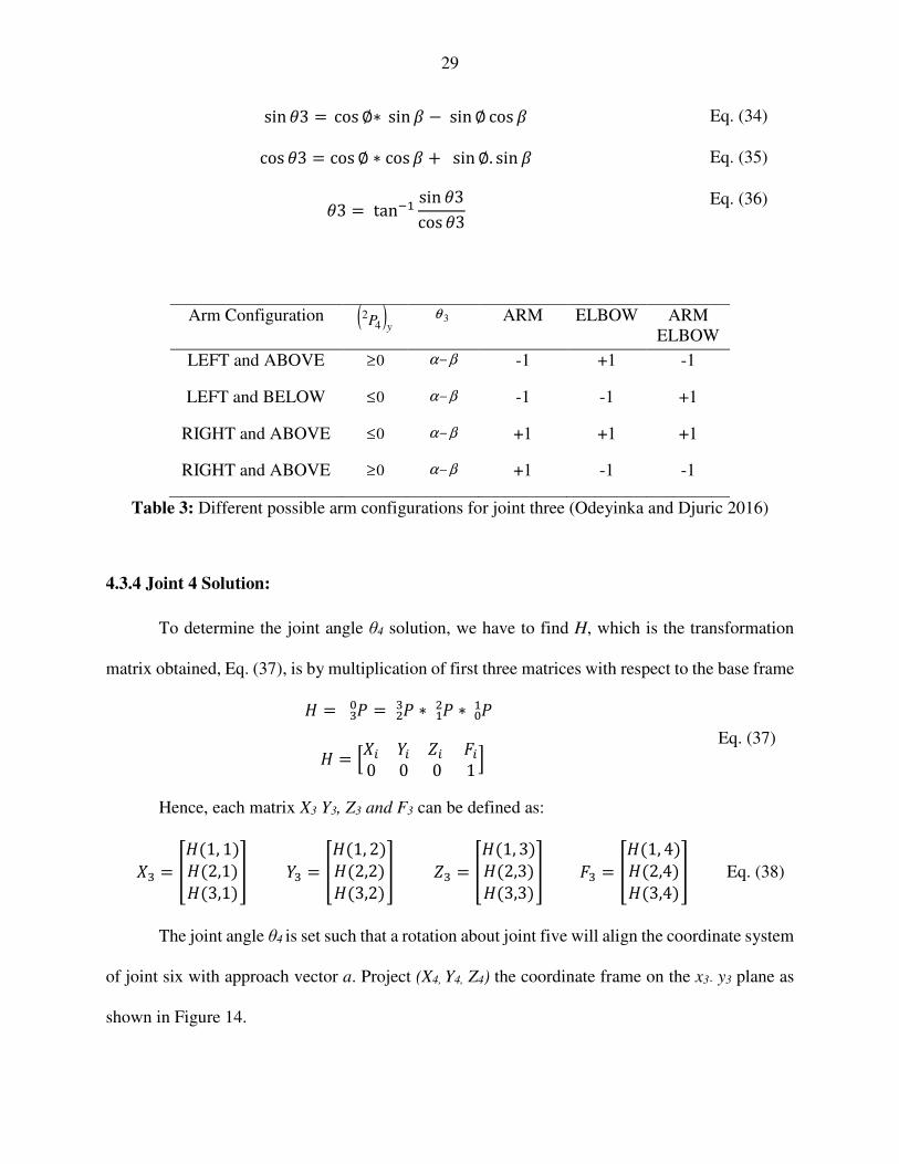
The joint angle θ4 is set such that a rotation about joint five will align the coordinate system
of joint six with approach vector a. Project (X4, Y4, Z4) the coordinate frame on the x3- y3 plane as
shown in Figure 14.
30
Figure 14: Rotation about joint five (Odeyinka and Djuric 2016)
In Figure 14, angle θ4 is geometrically represented, in the positive joint direction. The
detailed calculation for joint four, an angular displacement of Z3 by rotating along approach vector
Z4 resultant matrix is obtained, Eq. (40). The transpose the matrix for approach vector, a is given
by Eq. (39) as:
d567e Eq. (39)
= = ∗ Eq. (40)
We have Z4, X3 from Eqn. (38) - (40), that are used to calculate the sine and cosine values
of θ4 expressed in Eq. (41) and (42) and value of θ4 is calculated as inverse tan ratio, using
trigonometry and is expressed as Eq. (43)
sin = −(= ∙ `) Eq. (41)
cos = −(= ∙ a) Eq. (42)
= ftan sin cos g ∗ 180°$) Eq. (43)
3 5,x x
6x
3 5,y z ,C D
4θ4x
4z
4θ
Xbeam
Xls
31
There are following four solution cases of joint angle θ4, if the degenerate case occurs, any
convenient value may be used for as long as the orientation of the wrist (UP/DOWN) is satisfied
(Lee and Ziegler, 1984)
iftan sin cos g ∗ 180°$) j − 90°
Eq. (44)
= + O
= 90 − iftan sin cos g ∗ 180°$) j
= − 180°
The WRIST and Orientation of robot is defined by Eq. (46) - (47), Eq. (45) is assumed
= = −
a = = l = −a
Eq. (45)
Hence,
WRIST = sign( S ∙ Z) Eq. (46)
Orientation= Ω = l ∙ = Eq. (47)
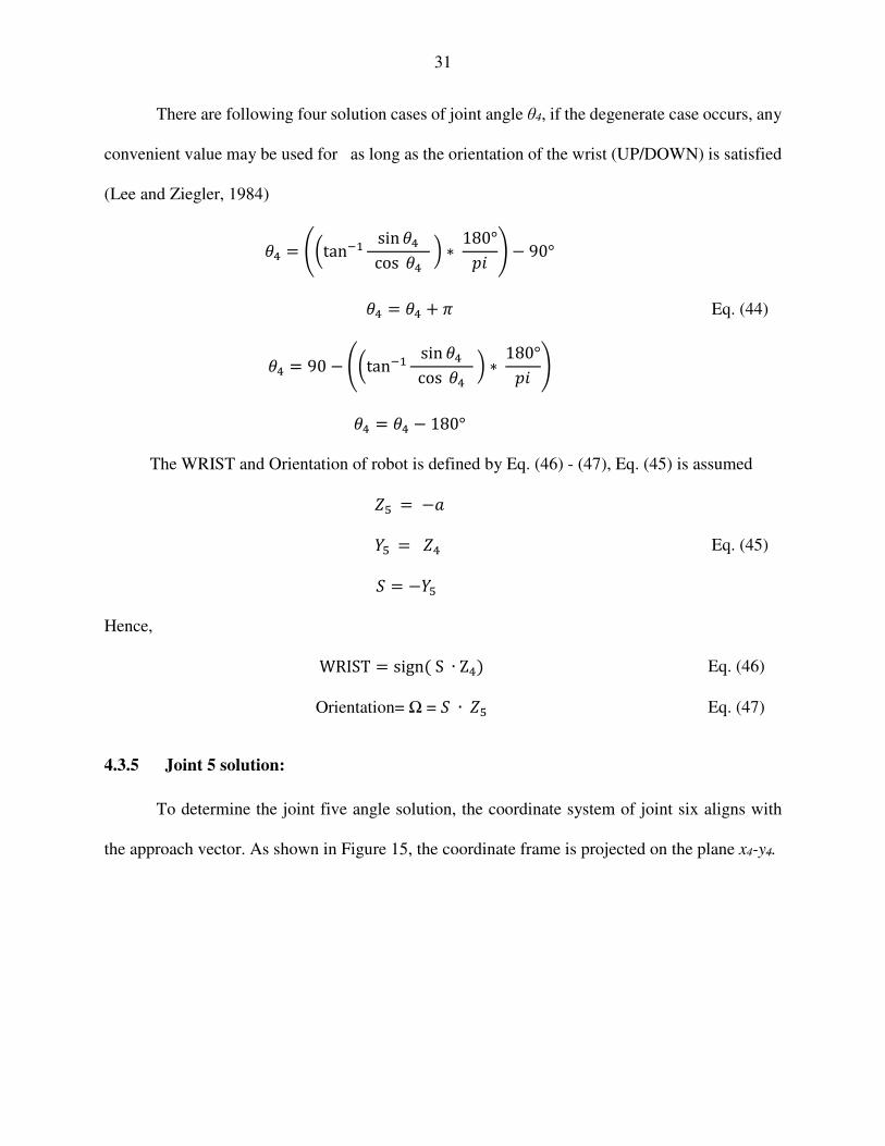
4.3.5 Joint 5 solution:
To determine the joint five angle solution, the coordinate system of joint six aligns with
the approach vector. As shown in Figure 15, the coordinate frame is projected on the plane x4-y4.
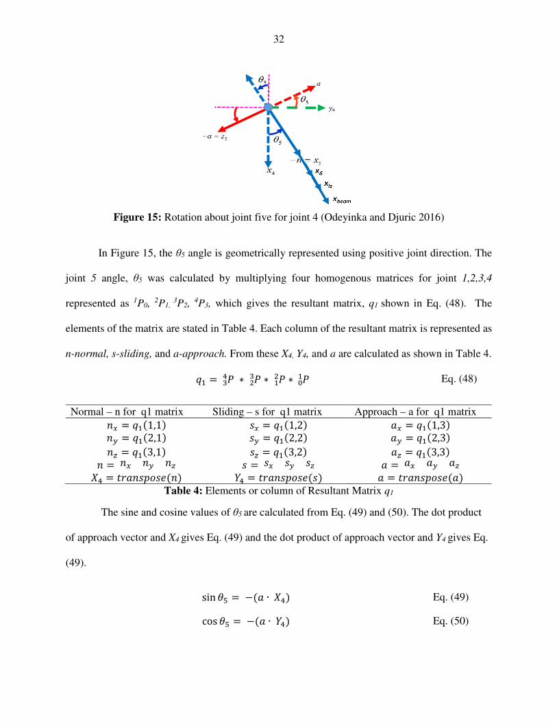
32
Figure 15: Rotation about joint five for joint 4 (Odeyinka and Djuric 2016)
In Figure 15, the θ5 angle is geometrically represented using positive joint direction. The
joint 5 angle, θ5 was calculated by multiplying four homogenous matrices for joint 1,2,3,4
represented as 1P0, 2P1, 3P2, 4P3, which gives the resultant matrix, q1 shown in Eq. (48). The
elements of the matrix are stated in Table 4. Each column of the resultant matrix is represented as
n-normal, s-sliding, and a-approach. From these X4, Y4, and a are calculated as shown in Table 4.
t ∗ ∗ ∗ Eq. (48)
Table 4: Elements or column of Resultant Matrix q1
The sine and cosine values of θ5 are calculated from Eq. (49) and (50). The dot product
of approach vector and X4 gives Eq. (49) and the dot product of approach vector and Y4 gives Eq.
(49).
sin 4 ∙ `8 Eq. (49)
cos 4 ∙ a8 Eq. (50)
Normal – n for q1 matrix Sliding – s for q1 matrix Approach – a for q1 matrix !5 t 41,18 #5 t 41,28 5 t 41,38 !6 t 42,18 #6 t 42,28 6 t 42,38 !7 t 43,18 #7 t 43,28 7 t 43,38 ! !5 !6 !7 # #5 #6 #7 5 6 7 ` uV!#$+#v4!8 a uV!#$+#v4#8 uV!#$+#v48
33
For the joint 5 solution θ5, is obtained from Eq. (51) by inverse tan ratio of Eq. (49) and
(50). If joint angle 5 obtained is θ5 = 0, then robot manipulator is said to be at singularity and
cannot be moved unless and until the θ5 is changed. The flip/no-flip configuration can be identified
by the sign of θ5. When θ5 is positive, it is in the flip configuration and when θ5 is negative, it is in
the no-flip configuration. All these configurations of joint 5 solutions as mentioned in Eq. (51)
180° ftan sin cos g ∗
180°$)
Eq. (51)
2 270° 270°
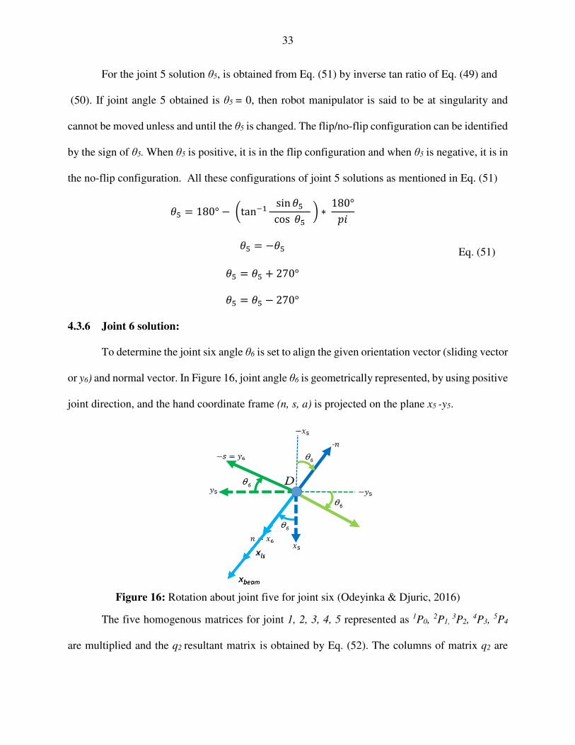
4.3.6 Joint 6 solution:
To determine the joint six angle θ6 is set to align the given orientation vector (sliding vector
or y6) and normal vector. In Figure 16, joint angle θ6 is geometrically represented, by using positive
joint direction, and the hand coordinate frame (n, s, a) is projected on the plane x5 -y5.
Figure 16: Rotation about joint five for joint six (Odeyinka & Djuric, 2016)
The five homogenous matrices for joint 1, 2, 3, 4, 5 represented as 1P0, 2P1, 3P2, 4P3, 5P4
are multiplied and the q2 resultant matrix is obtained by Eq. (52). The columns of matrix q2 are
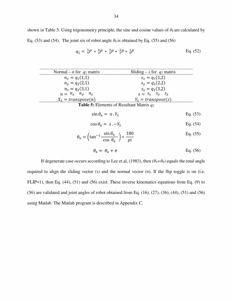
34
shown in Table 5. Using trigonometry principle, the sine and cosine values of θ6 are calculated by
Eq. (53) and (54). The joint six of robot angle θ6 is obtained by Eq. (55) and (56)
t ∗ ∗ ∗ ∗ Eq. (52)
Normal – n for q2 matrix Sliding – s for q2 matrix !5 = t(1,1) #5 = t(1,2) !6 = t(2,1) #6 = t(2,2) !7 = t(3,1) #7 = t(3,2) ! = !5 !6 !7 # = #5 #6 #7 ` = uV!#$+#v(!) a = uV!#$+#v(#) Table 5: Elements of Resultant Matrix q2 sin = ! . a Eq. (53)
cos = # . −a Eq. (54)
= ftan sin cos g ∗ 180$) Eq. (55)
= + O Eq. (56)
If degenerate case occurs according to Lee et.al, (1983), then (θ4+θ6) equals the total angle
required to align the sliding vector (s) and the normal vector (n). If the flip toggle is on (i.e.
FLIP=1), then Eq. (44), (51) and (56) exist. These inverse kinematics equations from Eq. (9) to
(56) are validated and joint angles of robot obtained from Eq. (16), (27), (36), (44), (51) and (56)
using Matlab. The Matlab program is described in Appendix C.
35
5. VALIDATION RESULTS FOR THE ALLS SYSTEM
5.1 Validation of Forward Kinematics for ALLS System
5.1.1 Fanuc robot S 430IW
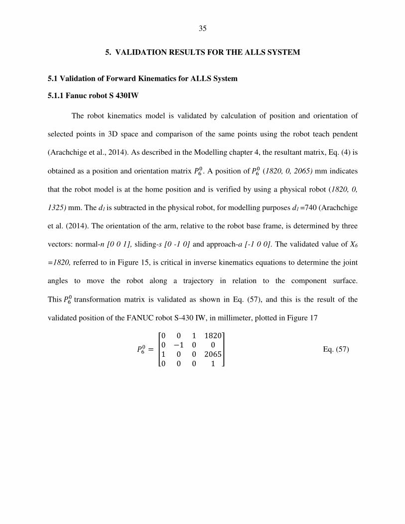
The robot kinematics model is validated by calculation of position and orientation of
selected points in 3D space and comparison of the same points using the robot teach pendent
(Arachchige et al., 2014). As described in the Modelling chapter 4, the resultant matrix, Eq. (4) is
obtained as a position and orientation matrix . A position of (1820, 0, 2065) mm indicates
that the robot model is at the home position and is verified by using a physical robot (1820, 0,
1325) mm. The d1 is subtracted in the physical robot, for modelling purposes d1 =740 (Arachchige
et al. (2014). The orientation of the arm, relative to the robot base frame, is determined by three
vectors: normal-n [0 0 1], sliding-s [0 -1 0] and approach-a [-1 0 0]. The validated value of X6
=1820, referred to in Figure 15, is critical in inverse kinematics equations to determine the joint
angles to move the robot along a trajectory in relation to the component surface.
This transformation matrix is validated as shown in Eq. (57), and this is the result of the
validated position of the FANUC robot S-430 IW, in millimeter, plotted in Figure 17
= (0 0 1 18200 −1 0 01 0 0 20650 0 0 1 , Eq. (57)
36
Figure 17: Validation of FANUC Robot S-430 IW model
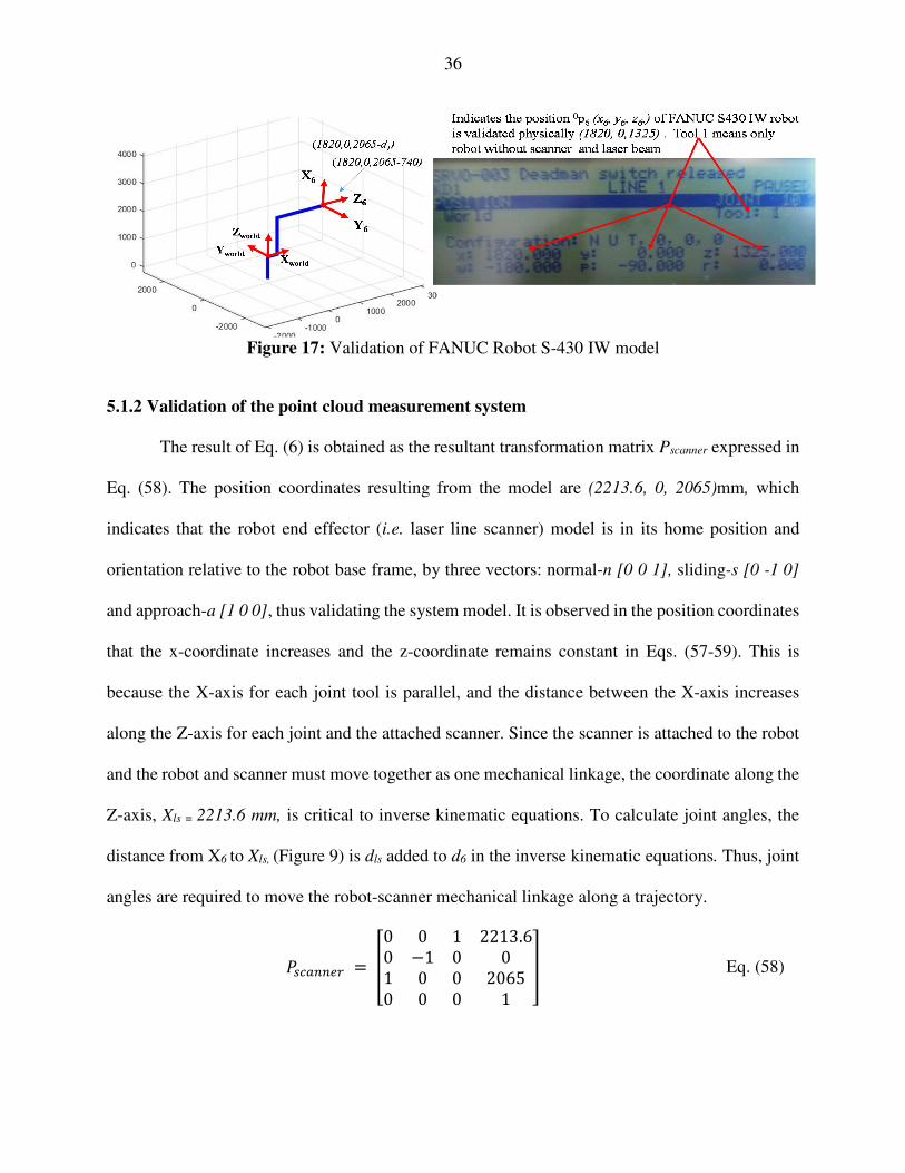
5.1.2 Validation of the point cloud measurement system
The result of Eq. (6) is obtained as the resultant transformation matrix Pscanner expressed in
Eq. (58). The position coordinates resulting from the model are (2213.6, 0, 2065)mm, which
indicates that the robot end effector (i.e. laser line scanner) model is in its home position and
orientation relative to the robot base frame, by three vectors: normal-n [0 0 1], sliding-s [0 -1 0]
and approach-a [1 0 0], thus validating the system model. It is observed in the position coordinates
that the x-coordinate increases and the z-coordinate remains constant in Eqs. (57-59). This is
because the X-axis for each joint tool is parallel, and the distance between the X-axis increases
along the Z-axis for each joint and the attached scanner. Since the scanner is attached to the robot
and the robot and scanner must move together as one mechanical linkage, the coordinate along the
Z-axis, Xls = 2213.6 mm, is critical to inverse kinematic equations. To calculate joint angles, the
distance from X6 to Xls, (Figure 9) is dls added to d6 in the inverse kinematic equations. Thus, joint
angles are required to move the robot-scanner mechanical linkage along a trajectory.
-.//0 = (0 0 1 2213.60 −1 0 01 0 0 20650 0 0 1 , Eq. (58)
37
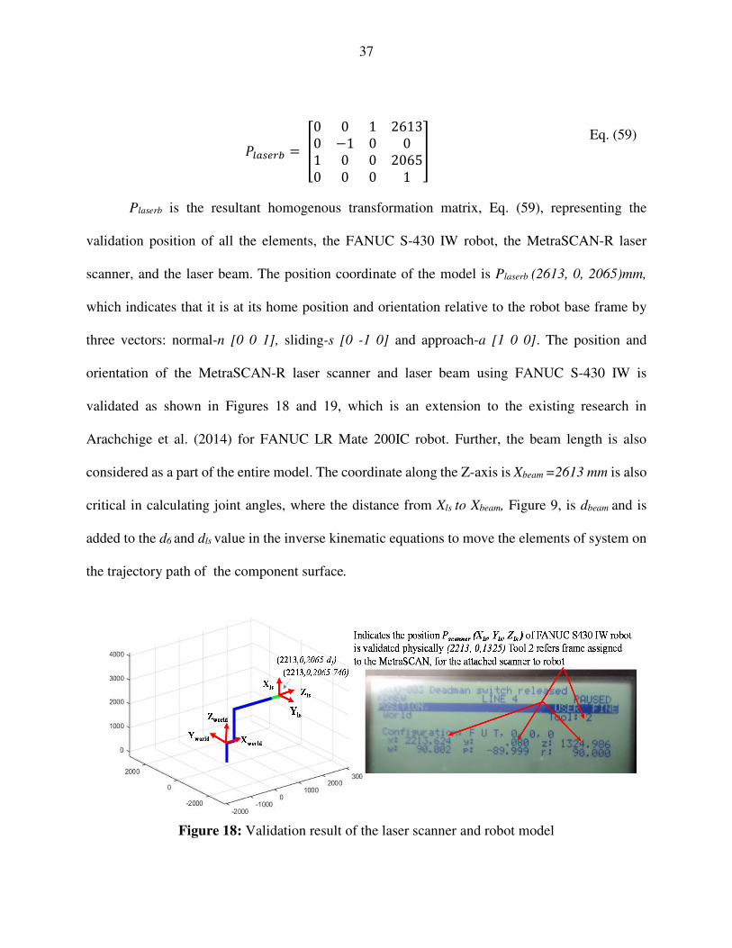
.0 = (0 0 1 26130 −1 0 01 0 0 20650 0 0 1 , Eq. (59)
Plaserb is the resultant homogenous transformation matrix, Eq. (59), representing the
validation position of all the elements, the FANUC S-430 IW robot, the MetraSCAN-R laser
scanner, and the laser beam. The position coordinate of the model is Plaserb (2613, 0, 2065)mm,
which indicates that it is at its home position and orientation relative to the robot base frame by
three vectors: normal-n [0 0 1], sliding-s [0 -1 0] and approach-a [1 0 0]. The position and
orientation of the MetraSCAN-R laser scanner and laser beam using FANUC S-430 IW is
validated as shown in Figures 18 and 19, which is an extension to the existing research in
Arachchige et al. (2014) for FANUC LR Mate 200IC robot. Further, the beam length is also
considered as a part of the entire model. The coordinate along the Z-axis is Xbeam =2613 mm is also
critical in calculating joint angles, where the distance from Xls to Xbeam, Figure 9, is dbeam and is
added to the d6 and dls value in the inverse kinematic equations to move the elements of system on
the trajectory path of the component surface.
Figure 18: Validation result of the laser scanner and robot model
38
Figure 19: Validation result of the measurement point cloud system
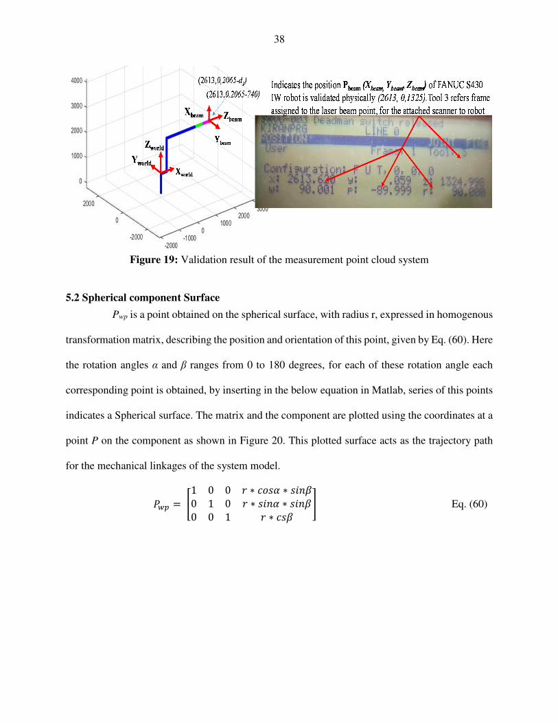
5.2 Spherical component Surface
Pwp is a point obtained on the spherical surface, with radius r, expressed in homogenous
transformation matrix, describing the position and orientation of this point, given by Eq. (60). Here
the rotation angles α and β ranges from 0 to 180 degrees, for each of these rotation angle each
corresponding point is obtained, by inserting in the below equation in Matlab, series of this points
indicates a Spherical surface. The matrix and the component are plotted using the coordinates at a
point P on the component as shown in Figure 20. This plotted surface acts as the trajectory path
for the mechanical linkages of the system model.
xy = d1 0 0 V ∗ *+# ∗ #)!S0 1 0 V ∗ #)! ∗ #)!S0 0 1 V ∗ *#S e Eq. (60)
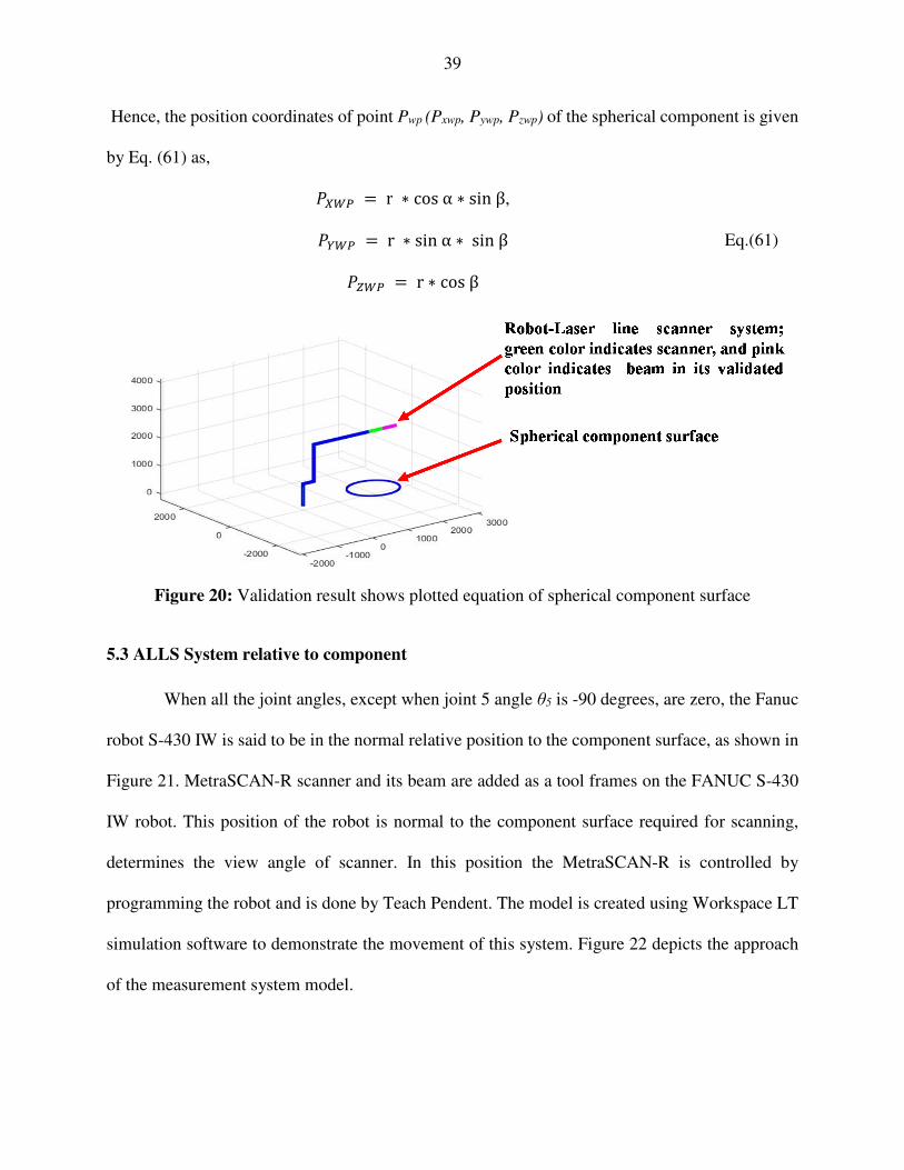
39
Hence, the position coordinates of point Pwp (Pxwp, Pywp, Pzwp) of the spherical component is given
by Eq. (61) as,
z| r ∗ cosα ∗ sinβ,
| r ∗ sinα ∗ sinβ
| r ∗ cosβ
Eq.(61)
Figure 20: Validation result shows plotted equation of spherical component surface
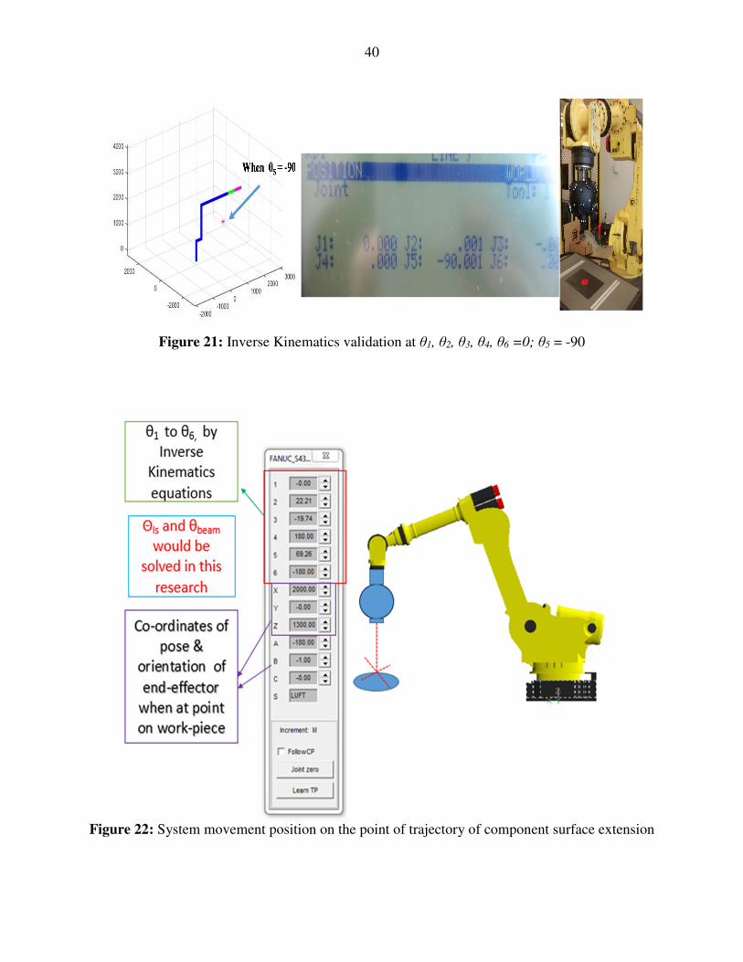
5.3 ALLS System relative to component
When all the joint angles, except when joint 5 angle θ5 is -90 degrees, are zero, the Fanuc
robot S-430 IW is said to be in the normal relative position to the component surface, as shown in
Figure 21. MetraSCAN-R scanner and its beam are added as a tool frames on the FANUC S-430
IW robot. This position of the robot is normal to the component surface required for scanning,
determines the view angle of scanner. In this position the MetraSCAN-R is controlled by
programming the robot and is done by Teach Pendent. The model is created using Workspace LT
simulation software to demonstrate the movement of this system. Figure 22 depicts the approach
of the measurement system model.
40
Figure 21: Inverse Kinematics validation at θ1, θ2, θ3, θ4, θ6 =0; θ5 = -90
Figure 22: System movement position on the point of trajectory of component surface extension
41
6. SCAN PATH EXPERIMENT & RESULTS
The forward and inverse kinematic equations are validated using FANUC S430 IW robot
and MetraSCAN-R system. As shown in Figure 17-19, where the resultant matrix was compared
with the teach pendant actual robot position, similarly, the ALLS system moving to the component
surface is validated along a particular trajectory path. The component surface is the spherical
scanner calibration plate the FANUC S-430 IW robot is moved to the point on the surface;
consequently the robot position is recorded. For this recorded position, the joint angles θ1, θ2, θ3,
θ4, θ5, θ6 are calculated to reach that measured point on the component surface. Each measured
point gives a certain position of the ALLS system and the joint angle values, which establish the
relation between the ALLS and the spherical component, and series of measured points gives a
trajectory path. To perform the experiment for scanning a trajectory path, following steps are
described: calibrating the robot, incorporating the safety limit on robot, setting a tool frame on
FANUC S430 IW, calibrating the C-track, MetraSCAN-R scanner, and movement of ALLS
system along a trajectory path.
6.1 Calibration of FANUC S-430 IW robot
The calibration of FANUC S-430 IW robot is usually required if the robot batteries needs
to be replaced or robot loses the power. The calibration steps are shown in the FANUC calibration
manual (FANUC America corporation Quick reference document). Using this manual we
performed the calibration using the Teach Pendent for FANUC S-430 IW described in Figures 23,
24, 25, and 26.
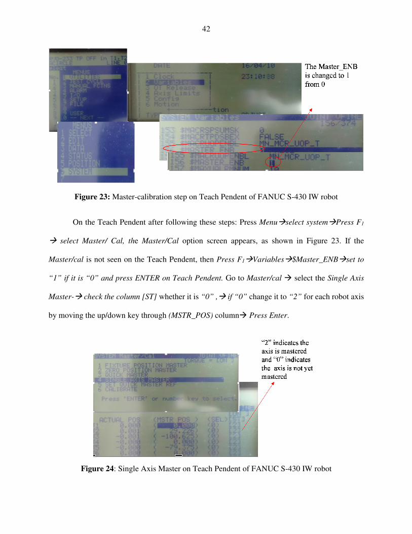
42
Figure 23: Master-calibration step on Teach Pendent of FANUC S-430 IW robot
On the Teach Pendent after following these steps: Press Menuselect systemPress F1
select Master/ Cal, the Master/Cal option screen appears, as shown in Figure 23. If the
Master/cal is not seen on the Teach Pendent, then Press F1Variables$Master_ENBset to
“1” if it is “0” and press ENTER on Teach Pendent. Go to Master/cal select the Single Axis
Master- check the column [ST] whether it is “0” , if “0” change it to “2” for each robot axis
by moving the up/down key through (MSTR_POS) column Press Enter.
Figure 24: Single Axis Master on Teach Pendent of FANUC S-430 IW robot
43
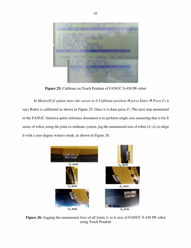
Figure 25: Calibrate on Teach Pendent of FANUC S-430 IW robot
In Master/Cal option move the cursor to 6 Calibrate position press Enter Press F4 it
says Robot is calibrated as shown in Figure 25. Once it is done press F5. The next step mentioned
in the FANUC America quick reference document is to perform single axis mastering that is for S
series of robot, using the joint co-ordinate system, jog the unmastered axis of robot (J1-J6) to align
it with a zero degree witness mark, as shown in Figure 26.
Figure 26: Jogging the unmastered Axis of all Joints J1 to J6 axis of FANUC S-430 IW robot using Teach Pendent
44
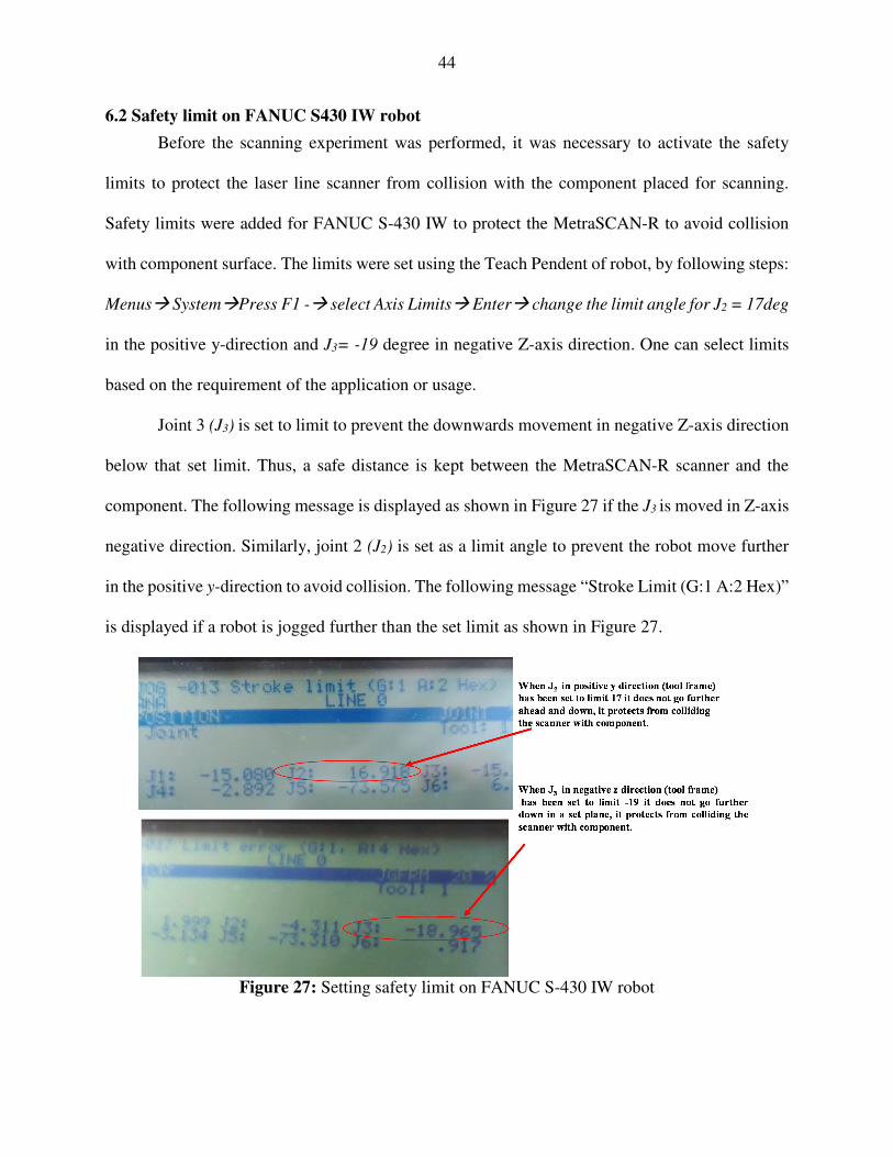
6.2 Safety limit on FANUC S430 IW robot
Before the scanning experiment was performed, it was necessary to activate the safety
limits to protect the laser line scanner from collision with the component placed for scanning.
Safety limits were added for FANUC S-430 IW to protect the MetraSCAN-R to avoid collision
with component surface. The limits were set using the Teach Pendent of robot, by following steps:
Menus SystemPress F1 - select Axis Limits Enter change the limit angle for J2 = 17deg
in the positive y-direction and J3= -19 degree in negative Z-axis direction. One can select limits
based on the requirement of the application or usage.
Joint 3 (J3) is set to limit to prevent the downwards movement in negative Z-axis direction
below that set limit. Thus, a safe distance is kept between the MetraSCAN-R scanner and the
component. The following message is displayed as shown in Figure 27 if the J3 is moved in Z-axis
negative direction. Similarly, joint 2 (J2) is set as a limit angle to prevent the robot move further
in the positive y-direction to avoid collision. The following message “Stroke Limit (G:1 A:2 Hex)”
is displayed if a robot is jogged further than the set limit as shown in Figure 27.
Figure 27: Setting safety limit on FANUC S-430 IW robot
45
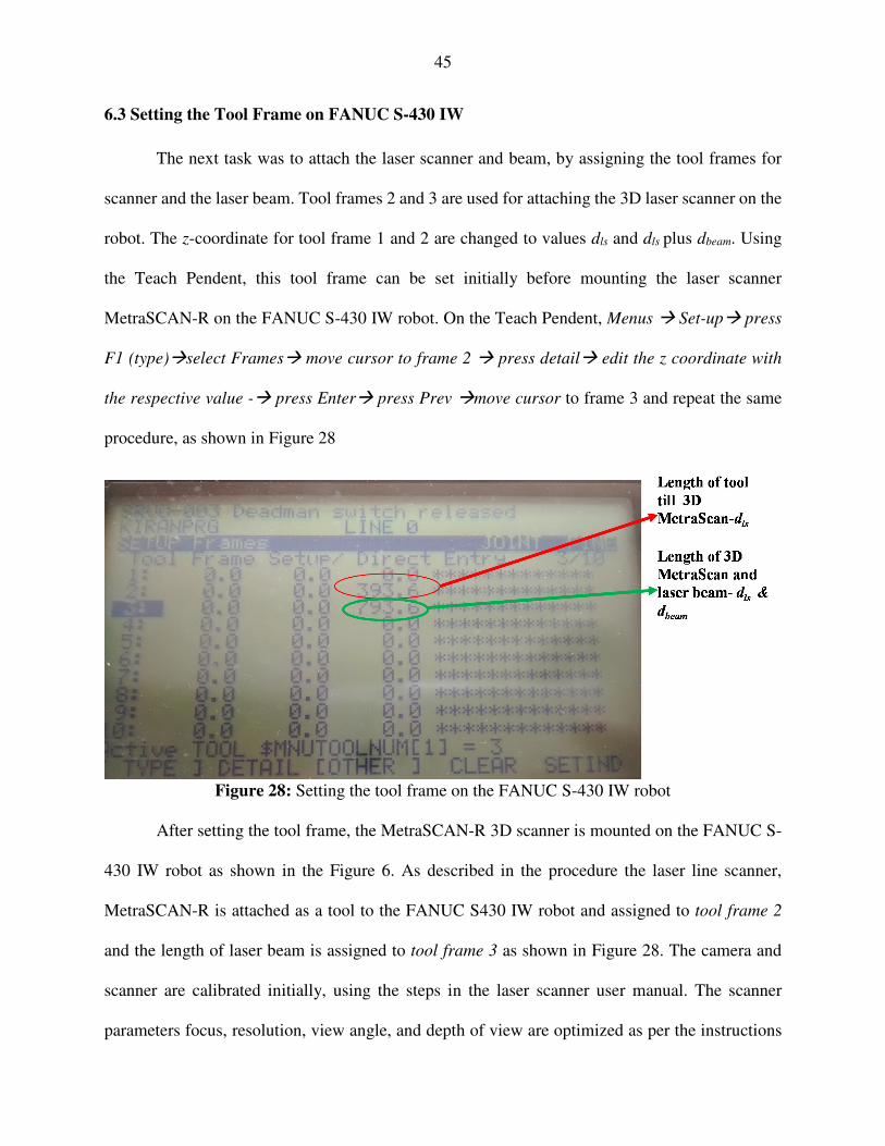
6.3 Setting the Tool Frame on FANUC S-430 IW
The next task was to attach the laser scanner and beam, by assigning the tool frames for
scanner and the laser beam. Tool frames 2 and 3 are used for attaching the 3D laser scanner on the
robot. The z-coordinate for tool frame 1 and 2 are changed to values dls and dls plus dbeam. Using
the Teach Pendent, this tool frame can be set initially before mounting the laser scanner
MetraSCAN-R on the FANUC S-430 IW robot. On the Teach Pendent, Menus Set-up press
F1 (type)select Frames move cursor to frame 2 press detail edit the z coordinate with
the respective value - press Enter press Prev move cursor to frame 3 and repeat the same
procedure, as shown in Figure 28
Figure 28: Setting the tool frame on the FANUC S-430 IW robot
After setting the tool frame, the MetraSCAN-R 3D scanner is mounted on the FANUC S-
430 IW robot as shown in the Figure 6. As described in the procedure the laser line scanner,
MetraSCAN-R is attached as a tool to the FANUC S430 IW robot and assigned to tool frame 2
and the length of laser beam is assigned to tool frame 3 as shown in Figure 28. The camera and
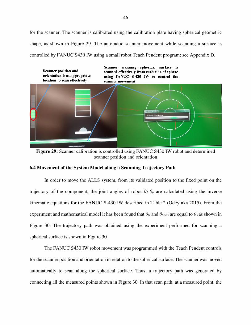
scanner are calibrated initially, using the steps in the laser scanner user manual. The scanner
parameters focus, resolution, view angle, and depth of view are optimized as per the instructions
46
for the scanner. The scanner is calibrated using the calibration plate having spherical geometric
shape, as shown in Figure 29. The automatic scanner movement while scanning a surface is
controlled by FANUC S430 IW using a small robot Teach Pendent program; see Appendix D.
Figure 29: Scanner calibration is controlled using FANUC S430 IW robot and determined
scanner position and orientation
6.4 Movement of the System Model along a Scanning Trajectory Path
In order to move the ALLS system, from its validated position to the fixed point on the
trajectory of the component, the joint angles of robot θ1-θ6 are calculated using the inverse
kinematic equations for the FANUC S-430 IW described in Table 2 (Odeyinka 2015). From the
experiment and mathematical model it has been found that θls and θbeam are equal to θ5 as shown in
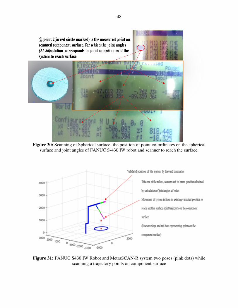
Figure 30. The trajectory path was obtained using the experiment performed for scanning a
spherical surface is shown in Figure 30.
The FANUC S430 IW robot movement was programmed with the Teach Pendent controls
for the scanner position and orientation in relation to the spherical surface. The scanner was moved
automatically to scan along the spherical surface. Thus, a trajectory path was generated by
connecting all the measured points shown in Figure 30. In that scan path, at a measured point, the

47
joint angles are shown representing the position (x, y, z) and orientation (Raw-Pitch-Yaw angle) of
the system with respect to the component surface. These joint angles indicate the position and
orientation of the system in order for the robot to reach the component surface. In this measurement
system, tool frames are set for combining the MetraSCAN-R 3D laser line scanner and its laser
beam on a FANUC S430 IW robot. Validation results obtained in Figure 18 and 19 provide the
relation between the FANUC S430 IW and MetraSCAN-R scanner. The result shown in Figure 20
provides the coordinates of the component surface. The calculation of joint angles shown in Figure
21 shows that this measurement system should be normal relative to the component surface point.
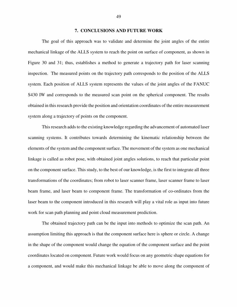
When the system is moved from point 2 to point 4 a trajectory path is scanned. Consequently, the
joint angles and actual coordinates of the system are obtained as shown in Figure 30. ALLS system
moves from the validation position to the new position as described in the Figure 31. Thus, the
non-contact inspection system, (FANUC S430 IW with MetraSCAN-R) acquires ‘as-is’
component spherical surface data, plans the trajectory path using the robot program, and obtains
the kinematic relationship between the robot, scanner, and fixed component surface without an
external measuring device. The objective to integrate three co-ordinate frames (the FANUC S430
IW robot, scanner, and component) while scanning a trajectory path (scan path) is achieved.
48
Figure 30: Scanning of Spherical surface: the position of point co-ordinates on the spherical
surface and joint angles of FANUC S-430 IW robot and scanner to reach the surface.
Figure 31: FANUC S430 IW Robot and MetraSCAN-R system two poses (pink dots) while
scanning a trajectory points on component surface
49
7. CONCLUSIONS AND FUTURE WORK
The goal of this approach was to validate and determine the joint angles of the entire
mechanical linkage of the ALLS system to reach the point on surface of component, as shown in
Figure 30 and 31; thus, establishes a method to generate a trajectory path for laser scanning
inspection. The measured points on the trajectory path corresponds to the position of the ALLS
system. Each position of ALLS system represents the values of the joint angles of the FANUC
S430 IW and corresponds to the measured scan point on the spherical component. The results
obtained in this research provide the position and orientation coordinates of the entire measurement
system along a trajectory of points on the component.
This research adds to the existing knowledge regarding the advancement of automated laser
scanning systems. It contributes towards determining the kinematic relationship between the
elements of the system and the component surface. The movement of the system as one mechanical
linkage is called as robot pose, with obtained joint angles solutions, to reach that particular point
on the component surface. This study, to the best of our knowledge, is the first to integrate all three
transformations of the coordinates; from robot to laser scanner frame, laser scanner frame to laser
beam frame, and laser beam to component frame. The transformation of co-ordinates from the
laser beam to the component introduced in this research will play a vital role as input into future
work for scan path planning and point cloud measurement prediction.
The obtained trajectory path can be the input into methods to optimize the scan path. An
assumption limiting this approach is that the component surface here is sphere or circle. A change
in the shape of the component would change the equation of the component surface and the point
coordinates located on component. Future work would focus on any geometric shape equations for
a component, and would make this mechanical linkage be able to move along the component of
50
any geometric shape. The obtained different position and orientation of the robot-laser scanning
system can be input for future work to develop the work-window for the FANUC S430 IW robot
and MetraSCAN-R scanning system.
The potential impact of this research thesis is its contribution to enhance the development
of optimization methods for laser line scan paths in order to collect best point clouds. ALLS
systems that can rapidly collect best point cloud datasets could become a viable inspection method
in production systems and transform inspection, quality monitoring, and core condition assessment
processes. Manufacturing quality monitoring systems would be provided with data and
information that significantly exceeds manual inspection or traditional Coordinate Measurement
Machines (CMMS). Remanufacturing condition assessment systems would benefit from an
advanced system that can accurately and quickly determine the condition of an end-of-use
component and develop as-is CAD models for remanufacturing planning of components.
The work of this thesis has been accepted to the 2016 North American Manufacturing
Research Conference and submitted to the 2016 Proceedings for NAMRI or SME Journal of
Manufacturing Systems.
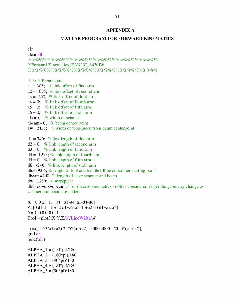
51
APPENDIX A
MATLAB PROGRAM FOR FORWARD KINEMATICS
clc clear all %%%%%%%%%%%%%%%%%%%%%%%%%%%%%%%%%% %Forward Kinematics_FANUC_S430IW %%%%%%%%%%%%%%%%%%%%%%%%%%%%%%%%%% % D-H Parameters a1 = 305; % link offset of first arm a2 = 1075; % link offset of second arm a3 = -250; % link offset of third arm a4 = 0; % link offset of fourth arm a5 = 0; % link offset of fifth arm a6 = 0; % link offset of sixth arm als =0; % width of scanner abeam= 0; % beam center point aw= 2438; % width of workpiece from beam centerpoint d1 = 740; % link length of first arm d2 = 0; % link length of second arm d3 = 0; % link length of third arm d4 = -1275; % link length of fourth arm d5 = 0; % link length of fifth arm d6 =-240; % link length of sixth arm dls=393.6; % length of tool and handle till laser scanner starting point dbeam=400; % length of laser scanner and beam dw= 1280; % workpiece d6b=d6+dls+dbeam % for inverse kinematics - d6b is considered as per the geometry change as scanner and beam are added X=[0 0 a1 a1 a1 a1-d4 a1-d4-d6] Z=[0 d1 d1 d1+a2 d1+a2-a3 d1+a2-a3 d1+a2-a3] Y=[0 0 0 0 0 0 0] Tool = plot3(X,Y,Z,'b','LineWidth',4) axis([-1.5*(a1+a2) 2.25*(a1+a2) -3000 3000 -200 3*(a1+a2)]) grid on hold('all') ALPHA_1 = (-90*pi)/180 ALPHA_2 = (180*pi)/180 ALPHA_3 = (90*pi)/180 ALPHA_4 = (-90*pi)/180 ALPHA_5 = (90*pi)/180
52
ALPHA_6 = (180*pi)/180 ALPHA_ls = (0*pi)/180 ALPHA_beam = (0*pi)/180 ALPHA_wp= (0*pi)/180 theta1_0 = 0 theta2_0 = -90 theta3_0 = 180 theta4_0 = 0 theta5_0 = 0 theta6_0 = 180 thetals_0 = 0 thetabeam_0 = 0 thetawp_0 = 0 %to be input using the Teach Pendent% theta1_Pendent = 0 theta2_Pendent = 0 theta3_Pendent = 0 theta4_Pendent = 0 theta5_Pendent = 0 theta6_Pendent = 0 thetals_Pendent = 0 thetabeam_Pendent= 0 thetawp_Pendent = 0 % conversion of joint angles to radians theta1 = (theta1_Pendent+theta1_0)*pi/180 theta2 = (theta2_Pendent+theta2_0)*pi/180 theta3 = (theta3_Pendent+theta3_0)*pi/180 theta4 = (theta4_Pendent+theta4_0)*pi/180 theta5 = (theta5_Pendent+theta5_0)*pi/180 theta6 = (theta6_Pendent+theta6_0)*pi/180 thetals = (thetals_Pendent+thetals_0)*pi/180 thetabeam =(thetabeam_Pendent+thetabeam_0)*pi/180 thetawp = (thetawp_0+thetawp_0)*pi/180 % homogenous matrices of robot six joints represented by %P1-P6 P1 = [cos(theta1), -cos(ALPHA_1)*sin(theta1), sin(ALPHA_1)*sin(theta1), a1*cos(theta1); sin(theta1), cos(ALPHA_1)*cos(theta1), -sin(ALPHA_1)*cos(theta1), a1*sin(theta1); 0, sin(ALPHA_1), cos(ALPHA_1), d1; 0, 0, 0, 1 ] P2 = [cos(theta2), -cos(ALPHA_2)*sin(theta2), sin(ALPHA_2)*sin(theta2), a2*cos(theta2); sin(theta2), cos(ALPHA_2)*cos(theta2), -sin(ALPHA_2)*cos(theta2), a2*sin(theta2); 0, sin(ALPHA_2), cos(ALPHA_2), d2; 0, 0, 0, 1 ];
53
P3 = [cos(theta3), -cos(ALPHA_3)*sin(theta3), sin(ALPHA_3)*sin(theta3), a3*cos(theta3); sin(theta3), cos(ALPHA_3)*cos(theta3), -sin(ALPHA_3)*cos(theta3), a3*sin(theta3); 0, sin(ALPHA_3), cos(ALPHA_3), d3; 0, 0, 0, 1 ]; P4 = [cos(theta4), -cos(ALPHA_4)*sin(theta4), sin(ALPHA_4)*sin(theta4), a4*cos(theta4); sin(theta4), cos(ALPHA_4)*cos(theta4), -sin(ALPHA_4)*cos(theta4), a4*sin(theta4); 0, sin(ALPHA_4), cos(ALPHA_4), d4; 0, 0, 0, 1 ]; P5 = [cos(theta5), -cos(ALPHA_5)*sin(theta5), sin(ALPHA_5)*sin(theta5), a5*cos(theta5); sin(theta5), cos(ALPHA_5)*cos(theta5), -sin(ALPHA_5)*cos(theta5), a5*sin(theta5); 0, sin(ALPHA_5), cos(ALPHA_5), d5; 0, 0, 0, 1 ]; P6 = [cos(theta6), -cos(ALPHA_6)*sin(theta6), sin(ALPHA_6)*sin(theta6), a6*cos(theta6); sin(theta6), cos(ALPHA_6)*cos(theta6), -sin(ALPHA_6)*cos(theta6), a6*sin(theta6); 0, sin(ALPHA_6), cos(ALPHA_6), d6; 0, 0, 0, 1 ]; %% Multiplication of six homogenous matrices P1_6 = P1*P2*P3*P4*P5*P6 %%% Plot validated robot joints 1-6%% HOME = plot3(P1_6(1,4), P1_6(2,4), P1_6(3,4), 'r*'); %%% Laser scanner attached as tool or end effector Pls= [cos(thetals), -cos(ALPHA_ls)*sin(thetals), sin(ALPHA_ls)*sin(thetals), als*cos(thetals); sin(thetals), cos(ALPHA_ls)*cos(thetals), -sin(ALPHA_ls)*cos(thetals), als*sin(thetals); 0, sin(ALPHA_ls), cos(ALPHA_ls), dls; 0, 0, 0, 1 ]; Pscanner= P1_6 *Pls %% Plot laser scanner %% Xls=[a1-d4-d6 a1-d4-d6+dls] Zls=[d1+a2-a3 d1+a2-a3] Yls =[0 0] Scanner = plot3(Xls,Yls,Zls,'g','LineWidth',4) FIRST = plot3(Pscanner(1,4), Pscanner(2,4), Pscanner(3,4), 'g*') %%Laser beam%% Pbeam= [cos(thetabeam), -cos(ALPHA_beam)*sin(thetabeam), sin(ALPHA_beam)*sin(thetabeam), abeam*cos(thetabeam); sin(thetabeam), cos(ALPHA_beam)*cos(thetabeam), -sin(ALPHA_beam)*cos(thetabeam), abeam*sin(thetabeam); 0, sin(ALPHA_beam), cos(ALPHA_beam), dbeam; 0, 0, 0, 1 ]; Plaserb=Pscanner*Pbeam %% Plot Laser beam %% Xb=[a1-d4-d6+dls a1-d4-d6+dls+dbeam]; Zb=[d1+a2-a3 d1+a2-a3]; Yb =[0 0]; beam = plot3(Xb,Yb,Zb,'m','LineWidth',4) SECOND = plot3(Plaserb(1,4), Plaserb(2,4), Plaserb(3,4), 'm*')
54
APPENDIX B
MATLAB PROGRAM FOR COMPONENT SURFACE
%% Plotting of component surface
r=635.8; Px= r*cos(ALPHA_wp)*sin(thetawp); Py= r*sin(ALPHA_wp)*sin(thetawp); Pz= r*cos(thetawp); X=[1 0 0 Px] Z=[0 0 1 Pz] Y=[0 1 0 Py] Tool1 = plot3(X+2000,Y, Z, 'r*') for i= 0:180 d = i *pi/180 for ALPHA_w = 0:d:180; for beta_w = 0:d:180; Pw =[cos(ALPHA_w)*cos(beta_w), -sin(ALPHA_w), cos(ALPHA_w)*sin(beta_w), r* cos(ALPHA_w)* sin(beta_w); sin(ALPHA_w)*cos(beta_w), cos(ALPHA_w), sin(ALPHA_w)*sin(beta_w), r*sin(ALPHA_w)*sin(beta_w); -sin(beta_w), 0, cos(beta_w),r*cos(beta_w); 0,0,0,1]; Envelope_1 = plot(Pw(1,4)+2000,Pw(3,4), 'b.') refreshdata(Tool1,'caller') drawnow pause(.1) end end end
55
APPENDIX C
MATLAB PROGRAM FOR INVERSE KINEMATICS
%%Inverse kinematics %% Using Samuel inverse kinematics for Fanuc family of robot for our FANUC S430 IW robot %% px6=P1_6(1,4) py6=P1_6(2,4) pz6=P1_6(3,4) ax= P1_6(1,3) ay=P1_6(2,3) az=P1_6(3,3) a=[ ax, ay, az] px =px6 -abs(d6)*a(1,1) py=py6-abs(d6)*a(1,2) pz=pz6-abs(d6)*a(1,3) %T4= P1*P2*P3*P4 %Px=T4(1,4) %Py=T4(2, 4) %Pz=T4(3,4) z0=[1 0 0] ARM=sign(dot(a,z0)) THETA1 = (atan2( Py,(ARM*Px)))*180/pi THETA1= THETA1+180 % Joint solution 2 r= sqrt(PX^2+py^2)-(a1*ARM) R = sqrt(r^2+(pz- abs(d1))^2) cos_betha=((a2)^2+R^2-(a3)^2-(d4)^2)/(2*R*(a2)) sin_betha=sqrt(1-(cos_betha)^2) sin_fi=-pz-abs(d1)/R cos_fi=-(r/R)*ARM ELBOW = ARM*sign(-d4*cos(theta3_Pendent)+a3*sin(theta3_Pendent)) sin_THETA2 = (sin_fi*cos_betha+ARM*ELBOW*cos_fi*sin_betha) cos_THETA2 = (cos_fi*cos_betha-ARM*ELBOW*sin_fi*sin_betha) THETA2 =((atan2(sin_THETA2,cos_THETA2)*180)/pi) THETA2 = theta2_0 - (atan2(sin_THETA2,cos_THETA2)*180/pi) THETA2 = theta2_0 + (atan2(sin_THETA2,cos_THETA2)*180/pi) A4=P3*P4 E= A4(2,4) ELBOW=ARM*sign (A4(2,4))
56
% joint 3 cos_fi=((a2)^2+(a3)^2+(d4)^2-(R)^2)/(2*(a2)*sqrt((a3)^2+(d4)^2)) sin_fi=ARM*ELBOW*sqrt(1-(cos_fi)^2) sin_betha=abs(d4)/sqrt((a3)^2+(d4)^2) cos_betha=abs(a3)/sqrt((a3)^2+(d4)^2) sin_THETA3= cos_fi*sin_betha-sin_fi*cos_betha cos_THETA3= cos_fi*cos_betha+sin_fi*sin_betha THETA3=((atan2(sin_THETA3,cos_THETA3)*180)/pi) THETA3_deg=THETA3-theta3_0 THETA3_deg=THETA3+theta3_0 % joint 4 solution H=P1*P2*P3 X3=H(1:3,1) y3=H(1:3,2) Z3=H(1:3,3) F3=H(1:3,4) a=transpose(a) Z4=(cross(Z3,a)) sin_THETA4=-(dot(Z4,X3)) cos_THETA4=(dot(Z4,y3)) THETA4= ((atan2(sin_THETA4,cos_THETA4)*180)/pi) THETA4= THETA4+180 THETA4= THETA4-90 THETA4= 90-((atan2(sin_THETA4,cos_THETA4)*180)/pi) THETA4= THETA4-180 % Derivation of Wrist configuration Z5=-a y5=Z4 S=-y5 WRIST= sign(dot(S,Z4)) %% joint 5 solution q1= P1*P2*P3*P4 nx=q1(1,1) ny=q1(2,1) nz=q1(3,1) n=[nx ny nz] % vector representing in x4 direction X4=transpose(n) sx=q1(1,2) sy=q1(2,2) sz=q1(3,2) s=[sx sy sz] % vector representing in y4 direction Y4= transpose(s)
57
ax=q1(1,3) ay=q1(2,3) az=q1(3,3) a=[ax,ay,az] % vector representing in z4 direction a=transpose(a) sin_THETA5= dot(-a, X4) cos_THETA5= dot(-a,Y4) THETA5=((atan2(sin_THETA5,cos_THETA5)*180)/pi) THETA5=180- ((atan2(sin_THETA5,cos_THETA5)*180)/pi) % joint 5 solution THETA5=-THETA5 THETA5=THETA5+270 THETA5=THETA5-270 % Joint 6 solution q2= P1*P2*P3*P4*P5 nx=q2(1,1) ny=q2(2,1) nz=q2(3,1) n=[nx ny nz] % vector representing in x4 direction X5=transpose(n) sx=q2(1,2) sy=q2(2,2) sz=q2(3,2) s=[sx sy sz] % vector representing in y4 direction Y5= transpose(s) sin_THETA6= dot(n,Y5) cos_THETA6= dot(s,-Y5) THETA6= ((atan2(sin_THETA6,cos_THETA6)*180)/pi) % Joint 6 solution THETA6= THETA6 + pi % when flip toggle is 1 or on % plotting of robot, scanner and beam again after calculating joint angles X=[0 0 a1 a1 a1-d4 a1-d4-d6b] Z=[0 d1 d1 d1+a2 d1+a2-a3 d1+a2-a3 d1+a2-a3] Y=[0 0 0 0 0 0 0] Tool = plot3(X,Y,Z,'b','LineWidth',4) axis([-1.5*(a1+a2) 2.25*(a1+a2) -3000 3000 -200 3*(a1+a2)]) grid on hold('all') P1 = [cos(THETA1), -cos(ALPHA_1)*sin(THETA1), sin(ALPHA_1)*sin(THETA1), a1*cos(THETA1); sin(THETA1), cos(ALPHA_1)*cos(THETA1), -sin(ALPHA_1)*cos(THETA1), a1*sin(THETA1); 0, sin(ALPHA_1), cos(ALPHA_1), d1; 0, 0, 0, 1 ]
58
P2 = [cos(THETA2), -cos(ALPHA_2)*sin(THETA2), sin(ALPHA_2)*sin(THETA2), a2*cos(THETA2); sin(THETA2), cos(ALPHA_2)*cos(THETA2), -sin(ALPHA_2)*cos(THETA2), a2*sin(THETA2); 0, sin(ALPHA_2), cos(ALPHA_2), d2; 0, 0, 0, 1 ] P3 = [cos(THETA3), -cos(ALPHA_3)*sin(THETA3), sin(ALPHA_3)*sin(THETA3), a3*cos(THETA3); sin(THETA3), cos(ALPHA_3)*cos(THETA3), -sin(ALPHA_3)*cos(THETA3), a3*sin(THETA3); 0, sin(ALPHA_3), cos(ALPHA_3), d3; 0, 0, 0, 1 ] P4 = [cos(THETA4), -cos(ALPHA_4)*sin(THETA4), sin(ALPHA_4)*sin(THETA4), a4*cos(THETA4); sin(THETA4), cos(ALPHA_4)*cos(THETA4), -sin(ALPHA_4)*cos(THETA4), a4*sin(THETA4); 0, sin(ALPHA_4), cos(ALPHA_4), d4; 0, 0, 0, 1 ] P5 = [cos(THETA5), -cos(ALPHA_5)*sin(THETA5), sin(ALPHA_5)*sin(THETA5), a5*cos(THETA5); sin(THETA5), cos(ALPHA_5)*cos(THETA5), -sin(ALPHA_5)*cos(THETA5), a5*sin(THETA5); 0, sin(ALPHA_5), cos(ALPHA_5), d5; 0, 0, 0, 1 ] P6 = [cos(THETA6), -cos(ALPHA_6)*sin(THETA6), sin(ALPHA_6)*sin(THETA6), a6*cos(THETA6); sin(THETA6), cos(ALPHA_6)*cos(THETA6), -sin(ALPHA_6)*cos(THETA6), a6*sin(THETA6); 0, sin(ALPHA_6), cos(ALPHA_6), d6; 0, 0, 0, 1 ] %% Multiplication of six homogenous matrices P1_6 = P1*P2*P3*P4*P5*P6 %%% Plot validated robot joints 1-6%% HOME = plot3(P1_6(1,4), P1_6(2,4), P1_6(3,4), 'r'); %%% Laser scanner attached as tool or end effector Pls= [cos(thetals), -cos(ALPHA_ls)*sin(thetals), sin(ALPHA_ls)*sin(thetals), als*cos(thetals); sin(thetals), cos(ALPHA_ls)*cos(thetals), -sin(ALPHA_ls)*cos(thetals), als*sin(thetals); 0, sin(ALPHA_ls), cos(ALPHA_ls), dls; 0, 0, 0, 1 ]; Pscanner= P1_6 *Pls %% Plot laser scanner %% Xls=[a1-d4-d6 a1-d4-d6+dls] Zls=[d1+a2-a3 d1+a2-a3] Yls =[0 0] Scanner = plot3(Xls,Yls,Zls,'g','LineWidth',4) FIRST = plot3(Pscanner(1,4), Pscanner(2,4), Pscanner(3,4), 'r') %%Laser beam%% Pbeam= [cos(thetabeam), -cos(ALPHA_beam)*sin(thetabeam), sin(ALPHA_beam)*sin(thetabeam), abeam*cos(thetabeam); sin(thetabeam), cos(ALPHA_beam)*cos(thetabeam), -sin(ALPHA_beam)*cos(thetabeam), abeam*sin(thetabeam); 0, sin(ALPHA_beam), cos(ALPHA_beam), dbeam; 0, 0, 0, 1 ]; Plaserb=Pscanner*Pbeam

59
%% Plot Laser beam %% Xb=[a1-d4-d6+dls a1-d4-d6+dls+dbeam]; Zb=[d1+a2-a3 d1+a2-a3]; Yb =[0 0]; beam = plot3(Xb,Yb,Zb,'m','LineWidth', 4) SECOND = plot3(Plaserb(1,4), Plaserb(2,4), Plaserb(3,4), 'm*')
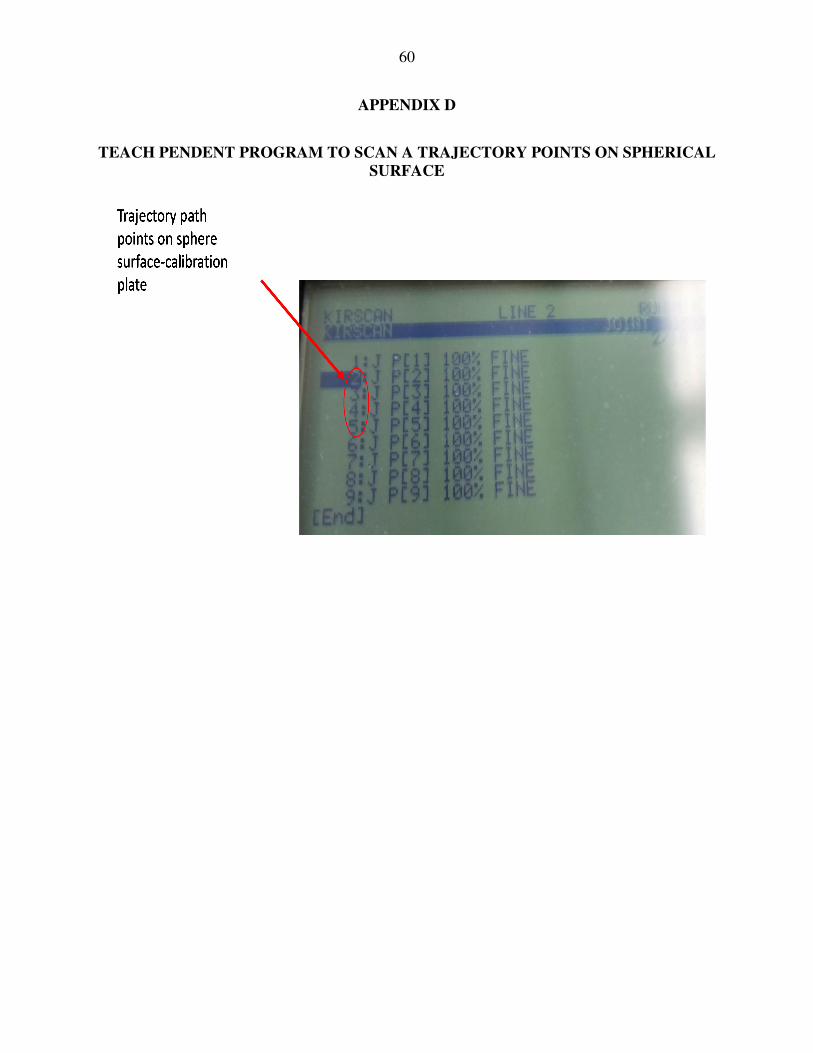
60
APPENDIX D
TEACH PENDENT PROGRAM TO SCAN A TRAJECTORY POINTS ON SPHERICAL
SURFACE
61
REFERENCES
Arachchige, P., Abderrahmane, M., & Djuric, A. M. Modeling and Validation of Rapid
Prototyping Related Available Workspace. SAE International Journal of Materials and
Manufacturing, 2014, 7, 291-299.
Bračun, D., Jezeršek, M., & Diaci, J. Triangulation Model Taking into Account Light Sheet
Curvature. Measurement Science and Technology, 2006, 17:2191.
Borangiu, T., Dogar, A., & Dumitrache, A. A heuristic approach for constrained real time motion
planning of a redundant 7-dof mechanism for 3D laser scanning. Paper presented at the
Information Control Problems in Manufacturing. 13th IFAC Symp. on Information Control
Problems in Manufacturing-INCOM,2009.
Buchsbaum, F., & Freudenstein, F. Synthesis of kinematic structure of geared kinematic chains
and other mechanisms. Journal of mechanisms, 1970, 5(3), 357-392.
Chen, C., Wang, Y., Ou, H., He, Y., & Tang, X. A review on remanufacture of dies and moulds.
Journal of Cleaner Production, 2014, 64,13-23.
Chow, J. Reproducing aircraft structural components using laser scanning. The International
Journal of Advanced Manufacturing Technology, 1997, 13(10), 723-728.
Decker, S. Dynamic Measurement of Position and Orientation of Robots. Instrumentation and
Measurement Technology Conference, 1992, 9th IEEE, 1990, 300-304
Denavit, J. A kinematic notation for lower-pair mechanisms based on matrices. Trans. of the
ASME. Journal of Applied Mechanics, 1955, 22, 215-221.
Denavit, R. Hartenberg. A Kinematic Notation for Lower-Pair Mechanisms Based on Matrices.
ASME Journal, 1955, 215-221.
62
Derigent, W., Chapotot, E., Ris, G., Remy, S., & Bernard. 3D digitizing strategy planning approach
based on a CAD model. Journal of computing and information science in engineering,
2007, 7(1), 10-19.
Djuric, A., & Urbanic,R. A Methodology for Defining the Functional Space (Work Window) for
a Machine Configuration. Paper presented at the 3ndInternational Conference on
Changeable, Agile, Reconfigurable and Virtual Production, 2009.
Dornaika, F., & Horaud, R. Simultaneous robot-world and hand-eye calibration. Robotics and
Automation, IEEE Transactions on, 1998, 14(4), 617-622.
Durupt, A., Remy, S., Ducellier, G., & Eynard, B. From a 3D point cloud to an engineering CAD
model: a knowledge-product-based approach for reverse engineering. Virtual and Physical
Prototyping, 2008, 3(2), 51-59.
ElMaraghy, H. & Yang, X. Computer-aided Planning of Laser Scanning of Complex Geometries.
CIRP Annals-Manufacturing Technology, 2003, 52(1):411-414.
FANUC America Corporation Quick Reference Document
Feng, H.-Y., Liu, Y., & Xi, F. Analysis of digitizing errors of a laser scanning system.Precision
Engineering, 2001, 25(3), 185-191
Fernández, P., Rico, J. C., Álvarez, B. J., Valiño, G., & Mateos, S. Laser scan planning based on
visibility analysis and space partitioning techniques. The International Journal of
Advanced Manufacturing Technology, 2008, 39(7-8), 699-715.
Fu, K. S., Gonzalez, R., & Lee, C. G. Robotics: Control Sensing. Vis: Tata McGraw-Hill
Education, 1987.
63
Haapala, K. R., Zhao, F., Camelio, J., Sutherland, J. W., Skerlos, S. J., Dornfeld, D. A., . . . Rickli,
J. L. A review of engineering research in sustainable manufacturing. Journal of
manufacturing science and engineering, 2013, 135(4), 041013.
Jin, X., & Yang, X. Off-line Programming of a Robot for Laser Re-manufacturing. Tsinghua
Science & Technology, 2009, 14(s1):186-191.
Kashani, A., Owen, W. S., Himmelman, N., Lawrence, P. D., & Hall, R. A. Laser Scanner-based
End-effector Tracking and Joint Variable Extraction for Heavy Machinery. The
International Journal of Robotics Research, 2010.
Kim, C., Espalin, D., Cuaron, A., Perez, M. A., Lee, M., MacDonald, E., & Wicker, R. B.
Cooperative Tool Path Planning for Wire Embedding on Additively Manufactured Curved
Surfaces Using Robot Kinematics. Journal of Mechanisms and Robotics, 2015, 7(2),
021003.
Kriegel, S., Bodenmüller, T., Suppa, M., & Hirzinger, G. A surface-based next-best-view approach
for automated 3D model completion of unknown objects. Paper presented at the Robotics
and Automation (ICRA), 2011 IEEE International Conference on., 2011
Kuş, A. Implementation of 3D optical scanning technology for automotive applications. Sensors,
2009, 9(3), 1967-1979.
Larsson, S. & Kjellander, J. Motion Control and Data Capturing for Laser Scanning with an
Industrial Robot. Robotics and Autonomous Systems, 2006, 54(6):453-460.
Larsson, S. & Kjellander, J. A. Path Planning for Laser Scanning with an Industrial Robot.
Robotics and Autonomous Systems, 2008, 56(7):615-624.
Lee, K. H., & Park, H.P. Automated Inspection Planning of Free-Form Shape Parts by Laser
scanning. Robotics and Computer-Integrated Manufacturing, 2000, 16(4):201-210.
64
Lee, C.S.G, & Ziegler M. A Geometric Approach in Solving The Inverse Kinematics of PUMA
Robots. Ann Arbor, Michigan, December 1983.
Leigh-Lancaster, C., Shirinzadeh, B. & Koh, Y. Development of a Laser Tracking System.
Mechatronics and Machine Vision in Practice, 1997. Proceedings., Fourth Annual
Conference on, 1997. IEEE, 163-168.
Lu, F., & Milios, E. Robot pose estimation in unknown environments by matching 2d range scans.
Journal of Intelligent and Robotic Systems, 1997,18(3), 249-275.
Mayer, J. R., & Parker. A portable instrument for 3-D dynamic robot measurements using
triangulation and laser tracking.Robotics and Automation, IEEE Transactions on, 1994,
10(4), 504-516.
Manocha, D., & Canny, J. F. Efficient inverse kinematics for general 6R manipulators. Robotics
and Automation, IEEE Transactions on, 1994, 10(5), 648-657.
Mehdi-Souzani, C., Thiébaut, F., & Lartigue, C. Scan planning strategy for a general digitized
surface. Journal of computing and information science in engineering, 2006, 6(4), 331-339.
Norman, A. R., Schonberg, A., Gorlach, I. A. & Schitt, R. Validation of Igps as an External
Measurement System for Cooperative Robot Positioning. The International Journal of
Advanced Manufacturing Technology, 2013, 64.1-4: 427-46.
Odeyinka, S. M. Complete Geometrical Approach to the Solution of Inverse Kinematics of
FANUC 6DOF Robot Families., Master Thesis, Wayne State University, 2015, 1-64.
Odeyinka, S. M., & Djuric, A. M. Fanuc Family Inverse Kinematics Modeling, Validation and
Visualization, 2016 (0148-7191).
Pieper, D.The kinematics of manipulators under computer control. PhD diss. Mechanical
Engineering Dept., Stanford Univ,1968.
65
Pauly, M., Mitra, N. J., & Guibas, L. J. Uncertainty and Variability in Point Cloud Surface Data.
Symposium on Point-based Graphics, 2004, 9.
Papaioannou, G., Karabassi, E.-A., & Theoharis, T. Reconstruction of three-dimensional objects
through matching of their parts. Pattern Analysis and Machine Intelligence, IEEE
Transactions on, 2002 24(1), 114-124.
Paoli, A., & Razionale, A. V. Large yacht hull measurement by integrating optical scanning with
mechanical tracking-based methodologies. Robotics and Computer-Integrated
Manufacturing, 2012, 28(5), 592-601.
Rickli, J. L., Dasgupta, A. K., & Dinda, G. P. A descriptive framework for additive
Remanufacturing systems. International Journal of Rapid Manufacturing, 2014, 4(2-4),
199-218.
Reinhart, G. & Tekouo, W. Automatic Programming of Robot-mounted 3D Optical Scanning
Devices to Easily Measure Parts in High-variant Assembly. CIRP Annals-Manufacturing
Technology, 2009, 58(1): 25-28.
Santolaria, J., Guillomía, D., Cajal, C., Albajez, J. A., & Aguilar, J. J. Modelling and calibration
technique of laser triangulation sensors for integration in robot arms and articulated arm
coordinate measuring machines.Sensors,2009, 9(9), 7374-7396.
Shiu, Y. C., & Ahmad, S. Calibration of wrist-mounted robotic sensors by solving homogeneous
transform equations of the form AX= XB. Robotics and Automation, IEEE Transactions
on, 1989, 5(1), 16-29.
Shen, C. & Zhu, S. A Robotic System for Surface Measurement Via 3D Laser Scanner. In
Proceedngs of the 2nd International Conference on Computer Applications and System
Modeling, 2012, 21, Paris, France. Atlantis Press.
66
Son, S., Park, H., & Lee, K. H. Automated Laser Scanning System for Reverse Engineering and
Inspection. International Journal of Machine Tools and Manufacture, 2002, 42(8): 889-
897.
Surmann, H., Nüchter, A., & Hertzberg, J. (2003). An autonomous mobile robot with a 3D laser
range finder for 3D exploration and digitalization of indoor environments. Robotics and
Autonomous Systems, 2003, 45(3), 181-198.
Stamos, I., & Leordean, M. Automated feature-based range registration of urban scenes of large
scale. Paper presented at the Computer Vision and Pattern Recognition, 2003. Proceedings.
2003 IEEE Computer Society Conference on.
Triebel, R., Frank, B., Meyer, J., & Burgard, W. First Steps Towards a Robotic System for Flexible
Volumetric Mapping of Indoor Environments. Proc. of the 5th IFAC Symp. on Intelligent
Autonomous Vehicles, 2004.
Vincze, M., Prenninger, J. P., & Gander, H. A Laser Tracking System to Measure Position and
Orientation of Robot End Effectors Under Motion. The International Journal of Robotics
Research, 1994, 13.4: 305-314
Wu, X., & Hu, Y. An Optical Scanner Aided Flexible Restoration System. Paper presented at the
Intelligent System Design and Engineering Application (ISDEA), 2012 Second
International Conference on., 2012.
Wang, Z., Mastrogiacomo, L., Franceschini, F., & Maropoulos, P. Experimental comparison of
dynamic tracking performance of iGPS and laser tracker. The International Journal of
Advanced Manufacturing Technology, 2011, 56(1-4), 205-213.
Xi, F. & Shu, C. CAD-based path planning for 3-D line laser scanning. Computer-Aided Design,
1999, 31:7, 473-479.
67
Yin, S., Ren, Y., Guo, Y., Zhu, J., Yang, S., & Ye, S. Development and Calibration of an Integrated
3D Scanning System for High-accuracy Large-scale Metrology. Measurement, 2014, 54:
65-76.
Yau, H-T., & Menq, C-H. Automated CMM path planning for dimensional inspection of dies and
molds having complex surfaces. International Journal of Machine Tools and Manufacture,
1995, 35:6, 861-876.
Zheng, J., Li, Z., & Chen, X. Worn area modeling for automating the repair of turbine blades. The
International Journal of Advanced Manufacturing Technology, 2006, 29(9-10), 1062-1067.
Zhu, S., Guo, Y.-c., & Yang, P. Remanufacturing system based on totally automatic MIG surfacing
via robot. Journal of Central South University of Technology, 2005, 12(2), 129-132.
Zhu, S., Cui, P.-z., Shen, C.-d., & Guo, Y.-c.Scanner external calibration algorithm based on fixed
point in robot remanufacturing system. Journal of Central South University of Technology,
2005, 12(2), 133-137.
Zheng, W., Luca, M., Paul, M. & Fiorenzo, F. Experimental Comparison of Dynamic Tracking
Performance of iGPS and Laser Tracker. The International Journal of Advanced
Manufacturing Technology, 2011, 56.1-4: 205-13.

68
ABSTRACT
KINEMATIC MODELING OF AN AUTOMATED LASER LINE SCANNING SYSTEM
by
KIRAN SUNIL DESHMUKH
May 2016
Advisor: Dr. Jeremy Rickli
Major: Engineering Management
Degree: Master of Science
This research work describes the geometric coordinate transformation in an automated
laser line scanning system caused by movements required for scanning a component surface. The
elements of an automated laser scanning system (robot, laser line scanner, and the component
coordinate system) function as a mechanical linkage to obtain a trajectory on a component surface.
This methodology solves the forward kinematics, derives the component surface, and uses inverse
kinematic equations to characterize the movement of the entire automated scanning system on
point trajectory. To reach a point on the component, joint angles of robot have been calculated. As
a result, trajectory path is obtained. This obtained robot poses on point trajectory of the component
surface can be used as an input for future work that aims to develop optimal scan paths to collect
“best” point cloud datasets. This work contributes in laser scanning inspection of component
surfaces in manufacturing, remanufacturing, and reverse engineering applications.

69
AUTOBIOGRAPHICAL STATEMENT
I am Kiran Deshmukh, a graduate student in Engineering Management at Wayne State
University. I received my bachelor’s degree in Instrumentation and Control Engineering at the
University of Pune, India. I have worked in the manufacturing industry for a few years. I was
motivated by the research work of Dr. Jeremy L. Rickli to pursue this thesis work. During the past
two years, I developed expertise in Robotics and Matlab modeling. The work of this thesis has and
acceptance to the 2016 North American Manufacturing Research Conference (NAMRC). My
research has boosted my confidence and gives me the entry opportunity into the research area of
kinematics and remanufacturing. This work will help in my future jobs involving Matlab, and in
Quality Engineering and Industrial Automation. The work of this thesis has been accepted to the
2016 North American Manufacturing Research Conference and will be submitted to the SME
Journal of Manufacturing Systems.


