
University of California
Los Angeles
Joint Channel Estimation and DecodingFor Wireless Channels
A dissertation submitted in partial satisfaction
of the requirements for the degree
Doctor of Philosophy in Electrical Engineering
by
Christos Komninakis
2000

c Copyright by
Christos Komninakis
2000

The dissertation of Christos Komninakis is approved.
Gregory J. Pottie
Ali H. Sayed
Kirby A. Baker
Richard D. Wesel, Committee Chair
University of California, Los Angeles
2000
ii

To my family.
iii
TABLE OF CONTENTS
1 Introduction : : : : : : : : : : : : : : : : : : : : : : : : : : : : : : : : : 1
1.1 Overview of Wireless Channels . . . . . . . . . . . . . . . . . . . . . 2
1.2 Overview of Dissertation Topics . . . . . . . . . . . . . . . . . . . . 5
I TURBO-CODES IN FLAT FADING 8
2 Trellis Turbo-Codes and the Forward-Backward Algorithm : : : : : : : 9
3 Flat Rayleigh Fading : : : : : : : : : : : : : : : : : : : : : : : : : : : : 15
3.1 Markov model for the phase . . . . . . . . . . . . . . . . . . . . . . 16
3.2 Quantized phase estimation . . . . . . . . . . . . . . . . . . . . . . . 20
4 Algorithms for Joint Data and Channel Estimation : : : : : : : : : : : 25
4.1 Forward-Backward phase estimation . . . . . . . . . . . . . . . . . . 25
4.1.1 Supertrellis algorithm . . . . . . . . . . . . . . . . . . . . . 27
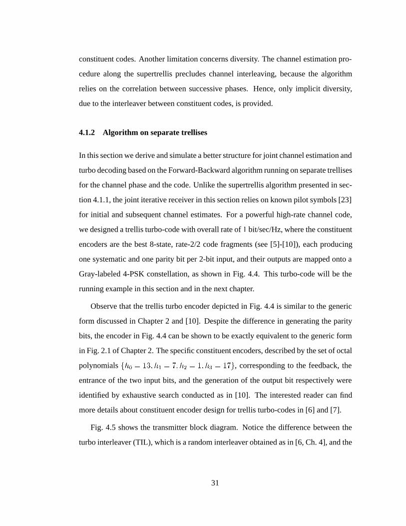
4.1.2 Algorithm on separate trellises . . . . . . . . . . . . . . . . . 31
4.2 Channel capacity . . . . . . . . . . . . . . . . . . . . . . . . . . . . 38
4.2.1 Simplified finite-state Markov channel (FSMC) model . . . . 38
4.2.2 Bounds on the capacity of a FSMC . . . . . . . . . . . . . . 40
4.2.3 Performance in the FSMC relative to capacity . . . . . . . . . 42
5 Diversity Reception in Flat Fading : : : : : : : : : : : : : : : : : : : : : 48
5.1 Transmission and channel model . . . . . . . . . . . . . . . . . . . . 49
iv
5.2 General iterative receiver . . . . . . . . . . . . . . . . . . . . . . . . 51
5.2.1 Quantized phase approach . . . . . . . . . . . . . . . . . . . 53
5.2.2 Optimum filtering approach . . . . . . . . . . . . . . . . . . 57
5.3 Simulation results . . . . . . . . . . . . . . . . . . . . . . . . . . . . 62
5.3.1 Capacity with receiver diversity . . . . . . . . . . . . . . . . 64
5.4 Conclusions . . . . . . . . . . . . . . . . . . . . . . . . . . . . . . . 67
II MIMO SYSTEMS IN FREQUENCY-SELECTIVE FADING 71
6 MIMO Frequency-Selective Channel : : : : : : : : : : : : : : : : : : : 72
6.1 Introduction . . . . . . . . . . . . . . . . . . . . . . . . . . . . . . . 72
6.2 MIMO channel model . . . . . . . . . . . . . . . . . . . . . . . . . 75
7 Receiver Structure and Performance : : : : : : : : : : : : : : : : : : : 81
7.1 Receiver structure . . . . . . . . . . . . . . . . . . . . . . . . . . . 81
7.1.1 Kalman tracking and channel prediction . . . . . . . . . . . 83
7.1.2 DFE design . . . . . . . . . . . . . . . . . . . . . . . . . . 85
7.2 Baseline adaptive systems . . . . . . . . . . . . . . . . . . . . . . . 88
7.3 Simulation results . . . . . . . . . . . . . . . . . . . . . . . . . . . 90
7.4 Coding . . . . . . . . . . . . . . . . . . . . . . . . . . . . . . . . . 96
7.5 Conclusions . . . . . . . . . . . . . . . . . . . . . . . . . . . . . . . 101
8 Conclusions and Future Work : : : : : : : : : : : : : : : : : : : : : : : 102
A Estimation from Pilot Symbols : : : : : : : : : : : : : : : : : : : : : : : 104
v

B Proof of Theorem 1 : : : : : : : : : : : : : : : : : : : : : : : : : : : : : 108
References : : : : : : : : : : : : : : : : : : : : : : : : : : : : : : : : : : : 111
vi
LIST OF FIGURES
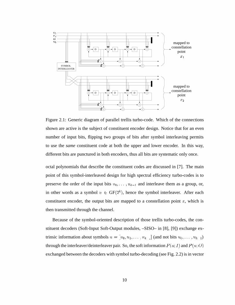
2.1 Generic diagram of parallel trellis turbo-code. . . . . . . . . . . . . . 10
2.2 Schematic diagram of the symbol turbo-decoder . . . . . . . . . . . . 14
3.1 Correlation coefficient for the amplitude and the phase of the fading
process fatg for fDT = 0:05. . . . . . . . . . . . . . . . . . . . . . . 17
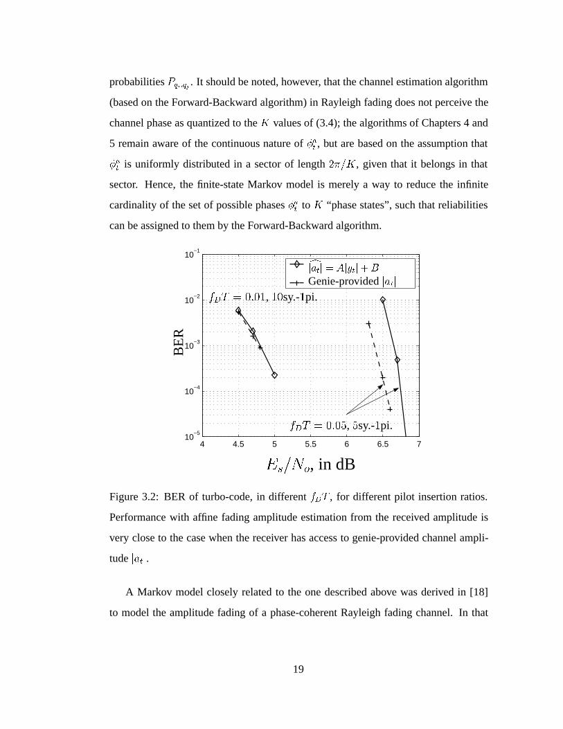
3.2 BER of turbo-code in different fDT , and for estimation vs. perfect
knowledge of amplitude fading. . . . . . . . . . . . . . . . . . . . . 19
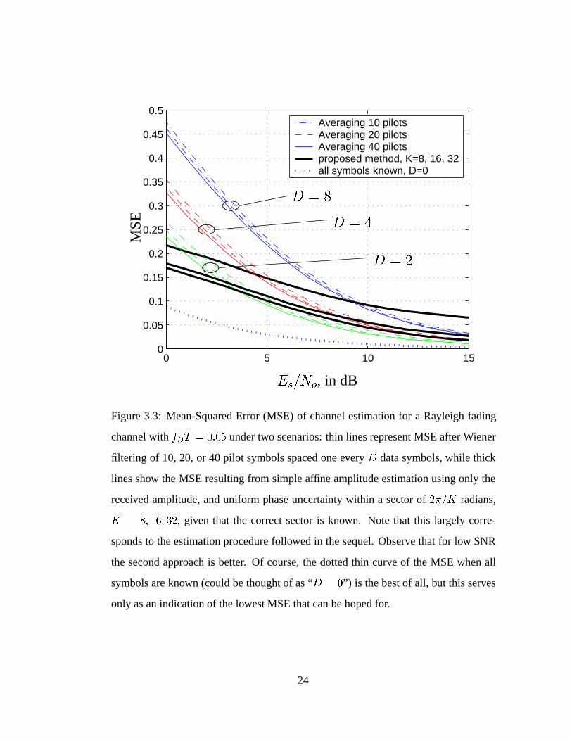
3.3 Mean-Squared Error (MSE) of channel estimation for a Rayleigh fad-
ing channel with fDT = 0:05 under two scenarios: optimum filtering
and knowledge of the correct quantized sector. . . . . . . . . . . . . . 24
4.1 Addition of angles in fading . . . . . . . . . . . . . . . . . . . . . . 26
4.2 Block diagram of system employing iterative decoder. . . . . . . . . . 27
4.3 Supertrellis and non-iterative pilot filtering performance in Clarke’s
channel with fDT = 0:05. . . . . . . . . . . . . . . . . . . . . . . . 29
4.4 The turbo-code used as a running example in this dissertation, with
overall rate of 1 bit/sec/Hz. . . . . . . . . . . . . . . . . . . . . . . . 32
4.5 Transmitter block diagram for pilot-aided turbo-code. . . . . . . . . . 32
4.6 Basic SISO building blocks of the receiver. . . . . . . . . . . . . . . 33
4.7 Receiver expansion in the processing time axis. . . . . . . . . . . . . 35
4.8 BER of turbo-code, for fDT = 0:01 and for different pilot insertion
ratios. . . . . . . . . . . . . . . . . . . . . . . . . . . . . . . . . . . 36
vii
4.9 BER of turbo-code, for fDT = 0:05 and for different pilot insertion
ratios. . . . . . . . . . . . . . . . . . . . . . . . . . . . . . . . . . . 37
4.10 Bounds on CFSMC for i.i.d. 4-PSK inputs. . . . . . . . . . . . . . . . 42
4.11 BER vs.Eb=No, for the turbo-code in the FSMC withK = 8 quantized
phases derived from fDT = 0:05. . . . . . . . . . . . . . . . . . . . 43
4.12 Capacity bounds and simulated BER in Markov channel for various
pilot insertion rates. . . . . . . . . . . . . . . . . . . . . . . . . . . . 44
5.1 Block diagram of the transmitter in a pilot-aided trellis turbo-coded
system. . . . . . . . . . . . . . . . . . . . . . . . . . . . . . . . . . 49
5.2 Flat fading channel with L branches of receiver diversity. . . . . . . . 50
5.3 Receiver block diagram for turbo-decoder with diversity and iterative
channel estimation. . . . . . . . . . . . . . . . . . . . . . . . . . . . 52
5.4 Transition probabilities for fDT = 0:05 (left) and fDT = 0:01 (right),
for K = 8 quantized phases. . . . . . . . . . . . . . . . . . . . . . . 54
5.5 BER of turbo-code, for fDT = 0:01 for the two channel estimation
methods, and given perfect CSI. . . . . . . . . . . . . . . . . . . . . 63
5.6 BER of turbo-code, for fDT = 0:05 for the two channel estimation
methods, and given perfect CSI. . . . . . . . . . . . . . . . . . . . . 64
5.7 Capacity (with Gaussian inputs) for i.i.d. Rayleigh fading channels
with receiver diversity orders of L = 1 and L = 2. Perfect channel
knowledge at the receiver is assumed. . . . . . . . . . . . . . . . . . 66
5.8 BER performance of turbo-code in flat Rayleigh fading with fDT =
0:01, with diversity orders of L = 2 and L = 1. . . . . . . . . . . . . 69
viii
5.9 BER performance of turbo-code in flat Rayleigh fading with fDT =
0:05, with diversity orders of L = 2 and L = 1. . . . . . . . . . . . . 70
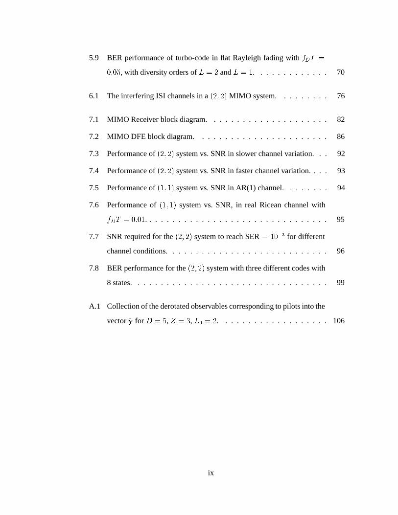
6.1 The interfering ISI channels in a (2; 2) MIMO system. . . . . . . . . 76
7.1 MIMO Receiver block diagram. . . . . . . . . . . . . . . . . . . . . 82
7.2 MIMO DFE block diagram. . . . . . . . . . . . . . . . . . . . . . . 86
7.3 Performance of (2; 2) system vs. SNR in slower channel variation. . . 92
7.4 Performance of (2; 2) system vs. SNR in faster channel variation. . . . 93
7.5 Performance of (1; 1) system vs. SNR in AR(1) channel. . . . . . . . 94
7.6 Performance of (1; 1) system vs. SNR, in real Ricean channel with
fDT = 0:01. . . . . . . . . . . . . . . . . . . . . . . . . . . . . . . . 95
7.7 SNR required for the (2; 2) system to reach SER = 10�3 for different
channel conditions. . . . . . . . . . . . . . . . . . . . . . . . . . . . 96
7.8 BER performance for the (2; 2) system with three different codes with
8 states. . . . . . . . . . . . . . . . . . . . . . . . . . . . . . . . . . 99
A.1 Collection of the derotated observables corresponding to pilots into the
vector ~y for D = 5, Z = 3, L0 = 2. . . . . . . . . . . . . . . . . . . 106
ix

LIST OF TABLES
4.1 Simulation results for the pilot-aided turbo-code in the FSMC derived
from fDT = 0:05. . . . . . . . . . . . . . . . . . . . . . . . . . . . . 46
x
Acknowledgments
As this work is coming to an end, I can only remember the good and joyous moments
of my graduate life at UCLA. The things I learned, including but certainly not limited
to receiver design and channel estimation, the people I met and the friends I made I
will cherish forever.
First and foremost, I want to extend my sincere thanks to my advisor, Professor
Rick Wesel, for making this period of time a pleasure. Since I joined his research
group (as a ”founding member”, so to speak) he has proven to be the best advisor a
student could ever hope for, with a passion for good, solid research work, persistence
for clear understanding and expression of both the questions and the answers, and a
level of energy and optimism that never ceases to amaze me. To those who thought that
the birth of his son, Kevin, (pictures of whom he shows prior to every presentation)
would slow him down a bit, he replied by almost doubling the size of our group. I
cannot thank him enough for the help, the encouragement, and those discussions that
boosted my understanding of the problems every single time. I am sure his influence
will serve me well in years to come, and wish I can have as rewarding a relationship
as I had with him with all the people I work with in the future.
To the older generation of Rick’s group, fellow-students Christina Fragouli, Xuet-
ing Liu and Wei Shi, thanks for the cooperation, the help, and the laughs on the sixth
floor of the Engineering Building. I wish them all the best for their personal and pro-
fessional lives. Particularly to Christina, I am grateful for the time we spent together,
as well as for the thoughts and discussions we have had, many of which can be found
in this dissertation.
To the newest members of the group, Mark Shane, Adina Matache, Cenk Kose and
Weidong (Tom) Sun, my best wishes: you are all in good hands, just keep hanging in
xi
there.
Sincere thanks also go to the members of my committee, Professors Kirby Baker,
Greg Pottie and Ali Sayed, who have taken time out of their busy schedules to attend
my Quals and read this dissertation. Professor Pottie’s insightful comments on my
prospectus helped improve my research work very much, and are greatly appreciated.
And Professor Sayed’s help and guidance in the second part of this dissertation were
invaluable; and his classes on estimation theory were a pleasure to attend. Also, many
thanks to Professor Lieven Vandenberghe for helping out on a specific optimization
problem and introducing me to non-linear programming.
I have enjoyed working (and taking breaks) in the same building as my friends
Peyman Meshkat (best wishes for his new business in Chicago) and Javier Garcia-
Frias (good luck in Delaware, with the tenure and the snow). Also, my thanks for
the good times to my soccer teammates Erik Berg, John Lach, Curt Schurgers, Mario
Novell (also my roomate for a while), Alexis Bernard, Hua Lu, Art Torosyan, Hanli
Zhou, Ranny Badra, Scott Siegrist and Matthieu Tisserand.
My good friends in LA, George Kondylis and his wife Tassoula helped me out a lot
when I first came to LA; I thank them for that, and wish them good luck at their new
home in northern California. To them and to Vaggelis Petsalis, thanks for the many
good times and their friendship, as well as for those amazing barbecue weekends.
Also, I want to thank my friends Harry Contopanagos and Sissy Kyriazidou, for all
their help and sharing the anxiety of the last few months. And to their little daughter
Leda, my best wishes.
To my close friends outside of LA, George Papadopoulos in New York and Kon-
stantis Adam in Berkeley, my thanks for putting up with me, both over the phone and
in person whenever I was dropping by; I have always appreciated the hospitality. And
to my buddies back in Greece, Panos Vassiliadis, Spyros Skiadopoulos, Pavlos Milas
xii

and Antonis Valakas, thanks for those emails that kept the group close from thousands
of miles apart.
Finally, not much would have been possible in my life without the love and un-
conditional support I receive from my family, my father Aristidis, my mother Maria
and brother George, as well as my grandmother Eirini. I know they are all proud of
me right now, and I love them all very much. My happiness associated with the com-
pletion of my graduate work is somewhat diminished by the fact that I cannot share it
with them. It is to them, my family, that I dedicate this dissertation.
xiii
Vita
1972 August 10: Born, Athens, Greece.
1990–1996 B.S. Electrical and Computer Engineering, National Technical Uni-
versity of Athens, Athens, Greece.
1997 Summer Intern, TI-DSP R&D, Texas Instruments, Dallas, TX.
1997–1998 Research Assistant, Electrical Engineering Department, UCLA.
1998 M.S. in Electrical Engineering, University of California at Los An-
geles, Los Angeles, CA.
1998–2000 Research Assistant, Electrical Engineering Department, UCLA.
2000 Ph.D. in Electrical Engineering, University of California at Los An-
geles, Los Angeles, CA.
PUBLICATIONS
C. Komninakis, C. Fragouli, A. H. Sayed, and R. D. Wesel, “Multi-Input Multi-Output
Fading Channel Tracking and Equalization using Kalman Estimation”, submitted to
IEEE Transactions on Signal Processing, November 2000.
C. Fragouli, C. Komninakis, and R. D. Wesel, “Minimality under Periodic Punctur-
ing”, submitted to International Conference on Communications, ICC 2001, Helsinki,
xiv
Finland, June 11-15, 2001.
C. Komninakis and R. D. Wesel, “Joint Iterative Channel Estimation and Decoding in
Flat Correlated Rayleigh Fading”, accepted to Journal on Selected Areas in Commu-
nications, special issue: The Turbo Principle - From Theory to practice.
C. Komninakis, C. Fragouli, A. H. Sayed, and R. D. Wesel, “Adaptive Multi-Input
Multi-Output Fading Channel Equalization using Kalman Estimation”, in Interna-
tional Conference on Communications, ICC 2000, New Orleans, Louisiana, June 18-
22, 2000.
C. Komninakis and R. D. Wesel, “Pilot-Aided Joint Data and Channel Estimation in
Flat Correlated Fading”, in Communication Theory Symposium of Globecom 99, Rio
de Janeiro, Brazil, December 5-9, 1999.
C. Komninakis, C. Fragouli, A. H. Sayed, and R. D. Wesel, “Channel Estimation and
Equalization in Fading”, in 33rd Asilomar Conference on Signals, Systems and Com-
puters, Pacific Grove, CA, October 24-27, 1999.
C. Komninakis, L. Vandenberge, and R. D. Wesel, “ Capacity of the Binomial Channel,
or Minimax Redundancy for Memoryless Sources”, (correspondence) submitted to
IEEE Transactions on Information Theory, November 2000.
C. Komninakis and R. D. Wesel, “Non-Pilot-Aided Iterative Decoding for Joint Data
Recovery and Channel Estimation in Fading” in 33rd Asilomar Conference on Signals,
Systems and Computers, Pacific Grove, CA, October 24-27, 1999.
xv
R. D. Wesel, X. Liu, C. Komninakis, and J. M. Cioffi, “Constellation Labeling for
Linear Encoders,” submitted to IEEE Transactions on Information Theory, submitted
April 1999.
C. Komninakis and R. D. Wesel, “Iterative Joint Channel Estimation and Decoding
in Flat Correlated Rayleigh Fading”, in 7th International Conference on Advances in
Communications and Control (COMCON), Athens, Greece, 28 June-2 July, 1999.
R. D. Wesel, C. Komninakis, and X. Liu, “Towards Optimality in Constellation Label-
ing”, in the proceedings of the Communication Theory Mini Conference at Globecom
97, Phoenix, AZ, November 3-8, 1997.
xvi
Abstract of the Dissertation
Joint Channel Estimation and DecodingFor Wireless Channels
by
Christos Komninakis
Doctor of Philosophy in Electrical Engineering
University of California, Los Angeles, 2000
Professor Richard D. Wesel, Chair
This dissertation is composed of two main parts. The first and largest part deals with
joint phase estimation and turbo-decoding in a flat Rayleigh fading channel. At the
region of low SNR where turbo-codes operate, and particularly if the variation of the
Rayleigh channel is quite large –i.e., large Doppler– the task of channel estimation
becomes quite challenging and should be done jointly with turbo-decoding for better
results. To this end, a Markov model is developed for a discretized version of the
channel phase (since this is a bigger problem for PSK transmission than amplitude
variation) and then the Forward-Backward algorithm is used on the phase trellis im-
plied by this Markov model to acquire the channel phase iteratively, while performing
turbo-decoding. Clearly, as the iterations proceed, the reliability of the coded symbols
increases, causing them to act somewhat as pilots and facilitate the phase estimation
process also.
This channel estimation scheme combines well with spectrally efficient trellis turbo-
codes and offers comparable performance to existing pilot averaging techniques at half
the bandwidth. To assess the proximity of the performance to channel capacity, upper
xvii
bounds to the capacity of idealized Markovian channel models are developed, and it is
demonstrated that performance as close as 1.3 dB from these upper bounds to capac-
ity without explicit CSI is possible. Also, this technique for iterative quantized phase
estimation is extended to the case where antenna diversity is available at the receiver,
and the performance improvement due to diversity is shown to be almost as much as
the increase in channel capacity.
The second part of this dissertation addresses joint channel estimation and equal-
ization for a general system with nT transmitter and nR receiver antennas, impaired
by co-channel interference and ISI. A Kalman filter is used to track the frequency-
selective channel, which is modeled as a first-order vector autoregressive process. The
Kalman filter is aided by delayed decisions from a MIMO m.m.s.e. DFE, which equal-
izes and decouples the transmitted signals, based on channel estimates received from
the Kalman filter. This approach works much better than conventional adaptive al-
gorithms such as LMS and RLS, at the expense of higher complexity. Furthermore,
suitable coding options for that equalization and interference cancellation scheme are
briefly discussed.
xviii
CHAPTER 1
Introduction
Research interest in the field of wireless communications has grown steadily in recent
years, and this trend is very likely to continue well into the future. From the physical
layer point of view, the goal is to devise schemes and techniques that increase the in-
formation rate and improve the robustness of a communication system under the harsh
conditions of the wireless environment. The wireless communication channel is the
source of various impairments to a digital communication system, due to factors such
as the relative mobility of transmitter and receiver, multipath propagation, interfer-
ence from other users of the frequency spectrum, and time-variation, more commonly
known as fading.
In this dissertation, based on widely accepted statistical models for the wireless
channel, we explore receiver design and algorithms aimed at combating the detrimen-
tal effects of wireless propagation. More specifically, the focus is on two relatively
recent advances in communication theory and practice, namely turbo-codes [1] and
the use of multiple transmitter and receiver antennas to boost the data rate [2]. Both
are treated here from the viewpoint of combining the procedures of channel estimation
with the decoding and equalization mechanisms respectively, something that is often
overlooked in the literature, relying on the assumption that channel state information
is somehow available at the receiver.
While this assumption might be reasonable in operating conditions of slow time-
variation and high signal-to-noise ratios (SNR), it is becoming increasingly outdated as
1
more powerful transmission and coding techniques emerge and broadband applications
require higher information rates. In those situations of low operating SNR and high
spectral efficiency, the channel estimation problem needs to be considered jointly with
that of decoding and equalization at the receiver. In particular, the iterative nature of
the turbo-decoding algorithm opens the possibility of integrating channel estimation
and decoder iterations, such that the two processes can benefit from each other. There
is great potential for performance improvement rather than obtaining one-shot channel
estimates and keeping the decoding process isolated.
For the problem of multiple antennas, this dissertation provides a solution to im-
prove the equalization and interference cancellation performance by allowing for knowl-
edge of largely invariant channel parameters to aid the estimation process, rather than
employing general adaptive equalization algorithms. Based on a first-order autoregres-
sive model for the MIMO channel time-variation, a Kalman filter is used to track the
channel and an finite MIMO decision-feedback equalizer (DFE) to equalize it, aided
by channel estimates from the Kalman filter and a prediction module.
1.1 Overview of Wireless Channels
For straightforward communication system design, an ideal channel is one that exhibits
constant frequency response over the transmission band, and thus produces an undis-
torted replica of the transmitted signal at the receiver, possibly delayed and scaled. In
other words, if the transmitted signal s(t) has an equivalent lowpass frequency repre-
sentation S(f), occupying total bandwidth W , then the equivalent lowpass frequency
response C(f) of an ideal channel is:
C(f) = jC(f)j � ej\C(f) = C � ej2��f (1.1)
2
for all frequencies in the band W of interest. If s(t) goes through the above ideal
channel, the received signal will be:
r(t) = C � s(t� �): (1.2)
Of course, real world transmission media, such as the mobile wireless channel,
have imperfections, which impair reliable transmission of information. The task of
the receiver becomes more complicated when those impairments are a priori unknown
and/or changing with time. Although the physical phenomena causing signal distor-
tion are very complex and often non-linear, their effects upon the transmitted signal
can be quite accurately modeled by a linear, possibly time-variant system. This dis-
sertation uses widely accepted linear, time-varying models of the wireless channel to
study various receiver structures, and lumps the effects of thermal and environmental
noise into the model as Additive White Gaussian Noise (AWGN).
The challenges posed by the wireless channel to digital communication are mainly
due to relative mobility of transmitter and receiver, coupled with multipath propaga-
tion. The net effects upon a transmitted pulse in general are dispersion and fading.
Dispersion refers to the widening in time of a transmitted pulse, causing it to overlap
with pulses transmitted at adjacent times, a phenomenon known as intersymbol inter-
ference (ISI). In the frequency domain this occurs when the transmission rate is high
enough, such that the transmitted bandwidth exceeds the coherence bandwidth of the
channel. So, if the transmission bandwidth is broad enough, the channel is bound to be
frequency-selective and thus dispersive. Fading describes the fluctuation of the signal
attenuation with time, which can be very severe and is due to motion or other changes
in the environment.
Significant time variability is not always associated with dispersion. In fact, at
lower transmission rates (narrowband transmission) the channel usually exhibits fast
time variation, but little frequency selectivity. This situation is described as flat fading,
3
whereby the channel introduces a time-varying attenuation that affects all frequency
components of the transmitted signal equally. For increasing transmission rates, the
fading is typically slower with respect to the transmission period, but the channel of-
ten becomes dispersive. Hence, in a relatively wideband transmission the channel
frequency response varies with frequency across the bandwidth of the digitally mod-
ulated signal (as well as in time), causing slowly time-varying ISI between adjacent
symbols, in what is called frequency-selective fading.
In broad terms, the time variability of a flat fading wireless channel depends on the
relative velocity between transmitter and receiver or moving scatterers in the environ-
ment, with respect to the transmission rate. A common way to quantify this is to refer
to the Doppler rate fDT , which is defined as the product of the maximum Doppler
frequency shift (fD) experienced by a mobile receiver and the transmission symbol
period T . Equivalently, this is the ratio of fD to the transmission baud rate.
Higher Doppler rates lead to faster varying channels, where the time correlation
between successive channel gains is smaller. Thus, the channel gain becomes less
than a specified level more often but stays at this low level (a fade) for a shorter time
duration. On the one hand, this increases the time diversity of the channel, which
can be exploited with coding and interleaving, because in a given time interval more
independent looks at the channel are available. On the other hand, faster variation
makes the task of channel estimation all the more difficult, particularly in a high-noise
environment, in which powerful channel codes –such as turbo-codes– operate. In the
limit of independent channel coefficients no estimation is possible.
For a frequency-selective fading channel the problem of time-variation, although
still significant, becomes less critical for two main reasons. First, as explained before,
the time-variation is usually slower with respect to the transmission rate. Second, one
more source of diversity, frequency diversity is available in this case, since different
4
parts of the transmitted power spectrum experience different attenuation due to the
frequency selective channel. One means to exploit frequency diversity is equalization,
whereby the goal of the receiver is to intelligently combine information carried by all
taps of the linear filter modeling the channel. When those taps are also time varying,
the equalizer has to adapt as the channel changes. Hence, for equalization of a time-
varying frequency-selective channel to be effective, accurate channel estimation and
tracking is required.
1.2 Overview of Dissertation Topics
In accordance with the basic distinction between flat and frequency-selective fading
channels outlined in the previous section, this dissertation consists of two main parts.
The first deals with joint channel estimation and turbo-decoding in a flat fading chan-
nel, and discusses ways to achieve reliable communication at rates close to channel
capacity, both with and without antenna diversity at the receiver. The second part
considers tracking and equalization (and, briefly, coding) for a frequency-selective
multi-input multi-output (MIMO) Ricean channel, whereby one or more antennas are
employed at the transmitter and receiver.
Chapter 2 briefly reviews symbol interleaved trellis turbo-codes and the Forward-
Backward algorithm used to decode them. This algorithm is a powerful tool that can
also be applied to estimation problems based on an appropriate hidden Markov model
(HMM). Chapter 3 introduces a widely accepted statistical model for the frequency-flat
Rayleigh fading channel encountered in narrowband transmission in a rich scattering
environment. Identifying acquisition of the channel phase as a more significant prob-
lem for PSK turbo-codes than amplitude fading leads to the introduction of a Markov
model that approximates both the values and the statistical properties of the fading
phase. Then, it is possible to construct a trellis representing this Markov phase model,
5
with states representing intervals of the continuous channel phase.
Building on those premises, Chapter 4 discusses algorithms for joint phase estima-
tion and turbo-decoding, using an adapted version of the Forward-Backward algorithm
as the phase estimation tool. Two main classes of algorithms are described and simu-
lated in various flat Rayleigh fading channels: a computationally intensive supertrellis,
combining the channel and code trellises into a supertrellis, and a more effective ap-
proach based on separate trellises that describe the channel and the constituent codes.
Performance is evaluated via simulation and also assessed in an absolute sense with
respect to channel capacity. For this purpose a sequence of progressively tighter upper
bounds on the constrained capacity of a purely Markov simplification to the Rayleigh
fading channel is derived, and performance of a turbo-code with joint iterative channel
estimation and decoding is demonstrated to approach these capacity bounds.
Chapter 5 extends the algorithms for joint phase estimation and turbo-decoding to
the case where antenna diversity of order L is available at the receiver. Performance
is assessed via simulations, and compared against performance achieved with itera-
tive optimum filtering for channel estimation. The discussion is again limited to flat
Rayleigh fading channels, and the performance gain due to receiver spatial diversity is
found to match the gain promised by the capacity improvement.
Finally, the second part of the dissertation (Chapters 6 and 7) addresses the problem
of channel tracking and equalization for multi-input multi-output (MIMO) time-variant
frequency-selective channels. These channels model the corrupting effects of inter-
symbol interference (ISI), co-channel interference (CCI), and noise. Chapter 6 derives
a first-order autoregressive model to describe the MIMO channel variation, such that
tracking can be performed by a Kalman filter.
Chapter 7 describes the proposed receiver, in which hard decisions to aid the
Kalman tracking algorithm come from a MIMO finite-length minimum-mean-squared-
6
error decision-feedback equalizer (MMSE-DFE), which performs the equalization task.
Since the optimum DFE for a wide range of channels produces decisions with a delay
� > 0, the Kalman filter tracks the channel with a delay. A channel prediction mod-
ule bridges the time gap between the channel estimates produced by the Kalman filter
and those needed for the DFE adaptation. The proposed algorithm offers good track-
ing behavior for multi-user fading ISI channels at the expense of higher complexity
than conventional adaptive algorithms. The coding problem for such a transmission
scenario is also briefly discussed. Applications include synchronous multiuser detec-
tion of independent transmitters, as well as coordinated transmission through many
transmitter/receiver antennas, for increased data rate.
Finally, Chapter 8 discusses how the work in both parts of this dissertation connects
with various areas of active research in the field of communication theory, particularly
in recent years. Also, the future work that will greatly enhance the results herein is
outlined.
The main contributions of the work presented in this dissertation are:
� A Markov model for the channel phase of a flat Rayleigh fading channel.
� Two algorithms for joint iterative phase estimation and turbo-decoding, also ap-
plicable when receiver diversity is available.
� A sequence of upper bounds on the capacity of systems with pilot assisted phase
estimation, based on the Markov phase model above.
� An algorithm for channel tracking and equalization of frequency-selective, multi-
ple-input multiple-output (MIMO) channels, based on Kalman estimation and
finite length MIMO MMSE DFE.
7

Part I
TURBO-CODES IN FLAT FADING
8
CHAPTER 2
Trellis Turbo-Codes and the Forward-Backward
Algorithm
Since their introduction [1] in 1993, parallel concatenated codes (in short “turbo-
codes”) and their variants, such as serially concatenated codes, have captured the in-
terest of the coding community and are being incorporated in the next generation of
standards. This is due to their impressive error correcting capabilities with reasonable
complexity, offering reliable communication within fractions of a dB from channel
capacity, at least in the AWGN channel [3], and in the perfectly interleaved, ideally
phase-coherent flat Rayleigh fading channel [4]. This dissertation examines the per-
formance of turbo-codes in flat Rayleigh fading, without assuming knowledge of the
channel at the receiver.
In particular, in an effort to achieve high spectral efficiency, this dissertation con-
centrates on trellis turbo-codes. In other words the transmitted signals are selected
from constellations of higher cardinality than BPSK. For completeness, Fig. 2.1 shows
a schematic diagram of a symbol-interleaved trellis turbo-code, designed following the
guidelines in [5].
The symbol interleaved turbo-codes used in this dissertation are special cases of the
diagram in Fig. 2.1. Whether a connection is active or not is determined by exhaustive
computer searches over all possible constituent encoders, as described in [5] and [6],
where tables of good constituent codes are given. The conventions about naming the
9
D D D
D D D
mapped toconstellation
point
mapped toconstellation
point
INTERLEAVERSYMBOL
u3u2u1u0
x1
x2
Figure 2.1: Generic diagram of parallel trellis turbo-code. Which of the connections
shown are active is the subject of constituent encoder design. Notice that for an even
number of input bits, flipping two groups of bits after symbol interleaving permits
to use the same constituent code at both the upper and lower encoder. In this way,
different bits are punctured in both encoders, thus all bits are systematic only once.
octal polynomials that describe the constituent codes are discussed in [7]. The main
point of this symbol-interleaved design for high spectral efficiency turbo-codes is to
preserve the order of the input bits u0; : : : ; uk�1 and interleave them as a group, or,
in other words as a symbol u 2 GF(2k), hence the symbol interleaver. After each
constituent encoder, the output bits are mapped to a constellation point x, which is
then transmitted through the channel.
Because of the symbol-oriented description of those trellis turbo-codes, the con-
stituent decoders (Soft-Input Soft-Output modules, –SISO– in [8], [9]) exchange ex-
trinsic information about symbols u = [u0; u1; : : : ; uk�1] (and not bits u0; : : : ; uk�1)
through the interleaver/deinterleaver pair. So, the soft informationP (u; I) and P (u;O)
exchanged between the decoders with symbol turbo-decoding (see Fig. 2.2) is in vector
10

form, because the symbols u 2 GF(2k) can take more than two values. In bit decod-
ing, scalars are enough to convey the log-likelihood ratio of each bit ui 2 GF(2). It
can be shown that symbol decoding is exactly equivalent to the bit-oriented decoding
of trellis turbo-codes described in [7], but devoid of the additional assumption that bits
within a symbol u 2 GF(2k) are conditionally independent given the whole observed
sequence. The absence of this implicit assumption in symbol turbo-decoding generally
improves performance [10], while the coding scheme of Fig. 2.1 eliminates puncturing
constraints placed on the constituent encoders and interleaver by [11].
In any case the basic tool for decoding is the Forward-Backward algorithm [12],
which is briefly described below. In its initial form in [12] this algorithm provides
maximum a posteriori (MAP) decoding of trellis codes, but its iterative use for the
decoding of turbo-codes has revived interest in it as a powerful estimation tool, not
only for codes but also for any hidden Markov model (HMM —see [13] and [14]). It
is an algorithm that operates on blocks of data.
Specifically, given the whole sequence yN1 of N observations fytgt=1;::: ;N from an
HMM with inputs u, states S 2 S = fm : m = 0; 1; : : : ; jSj � 1g and outputs x (the
y’s can be noisy observations of the coded symbols x from a code with inputs u), the
posterior probability of the input symbol ut at every time instant t is:
P (ut = ujyN1 ) = G � P (ut = u; yN1 ) = (2.1)
= G �X
(m0;m)2E(u)
P (St�1 = m0; St = m; y
N1 ) (2.2)
= G �X
(m0;m)2E(u)
8><>:P (St�1 = m0; y
t�11 )| {z }
�t�1(m0)
�P (St = m; ytj St�1 = m0)| {z }
t(m0;m)
�
P (yNt+1j St = m)| {z }�t(m)
9>=>; (2.3)
11
where G is an irrelevant constant G = 1=P (yN1 ), and:
E(u) = f(m0; m) : 9 state transition (St�1 = m
0 ! St = m) with input ut = ug(2.4)
is the set of transitions between states that produce the desired input symbol u. For
t = 1; : : : ; N; and for m = 0; 1; : : : ; jSj � 1, the “forward” variables at(m) and the
“backward” variables �t(m) are computed through the recursions:
�t(m) =Xm0
�t�1(m0) � t(m0
; m) (2.5)
�t(m) =Xm0
t+1(m;m0) � �t+1(m
0); (2.6)
For the above recursions, knowledge of the initial and final states S0 and SN is needed.
Thus, for every N -symbol block, the encoder is forced to terminate at the zero state,
which implies that for every block it is S0 = SN = 0. Therefore, the following
initialization of the forward and backward variables is necessary for the recursions:
�0(m) = Pr(S0 = m) =
8<: 1 if m = 0
0 otherwise(2.7)
In a similar fashion:
�N (m) = Pr(SN = m) =
8<: 1 if m = 0
0 otherwise(2.8)
For a single trellis code, (2.1) can be used to perform MAP decoding, but in the
iterative decoding of turbo-codes, sketched in Fig. 2.2, certain modifications are nec-
essary to preserve the independence of information used by constituent decoders as
much as possible. For straightforward MAP decoding of the symbol ut it is enough to
identify the u that maximizes the quantity:X(m0;m)2E(u)
�t�1(m0) � t(m0
; m) � �t(m): (2.9)
12
For the forward and backward recursions [9] for the �’s and �’s respectively, the cru-
cial quantity to be computed is:
t(m0; m) = Pr (St = m; yt j St�1 = m
0)
= Pr (St = mj St�1 = m0) � Pr (yt j St = m;St�1 = m
0) (2.10)
= Pr (u : St�1 = m0 ! St = m) � Pr (yt j x(m0 ! m)) ; (2.11)
where x(m0 ! m) is the output symbol of the code (or, in general, the noiseless
observable of the Hidden Markov Model) corresponding to the state transition m0 !m. Eq. (2.11) shows that t(m0
; m) is essentially the product of the probability of
the state transition and the probability of the observation given that the state transition
took place. When the algorithm is used iteratively, as in Fig. 2.2, the first part of (2.11)
is the extrinsic probability about the input, denoted P (u; I) in the literature [3] and
provided by the other constituent decoder.
While for MAP decoding of a single code, the same t(m0; m) (including the a
priori input probability term P (u; I)) is used both for the recursions (2.5)-(2.6) and for
the MAP decision (2.9), iterative symbol decoding of turbo-codes works differently:
P (u; I) is included in the t(m0; m) used to perform the recursions (2.5)-(2.6), but
is omitted when producing the updated extrinsic probability P (u;O) to be fed to the
other decoder. This is given by:
P (u;O) =X
(m0;m)2E(u)
�t�1(m0) � ~ t(m0
; m) � �t(m); (2.12)
where ~ t(m0; m) = Pr (yt j x(m0 ! m)). This avoids direct circulation of the same
soft information between the two constituent decoders.
Finally, note that for reasons of computational complexity and numerical stability
in practice the algorithm is not used in its multiplicative form outlined above. Instead,
logarithms of the quantities �, � and are used, and this allows additions to replace
13
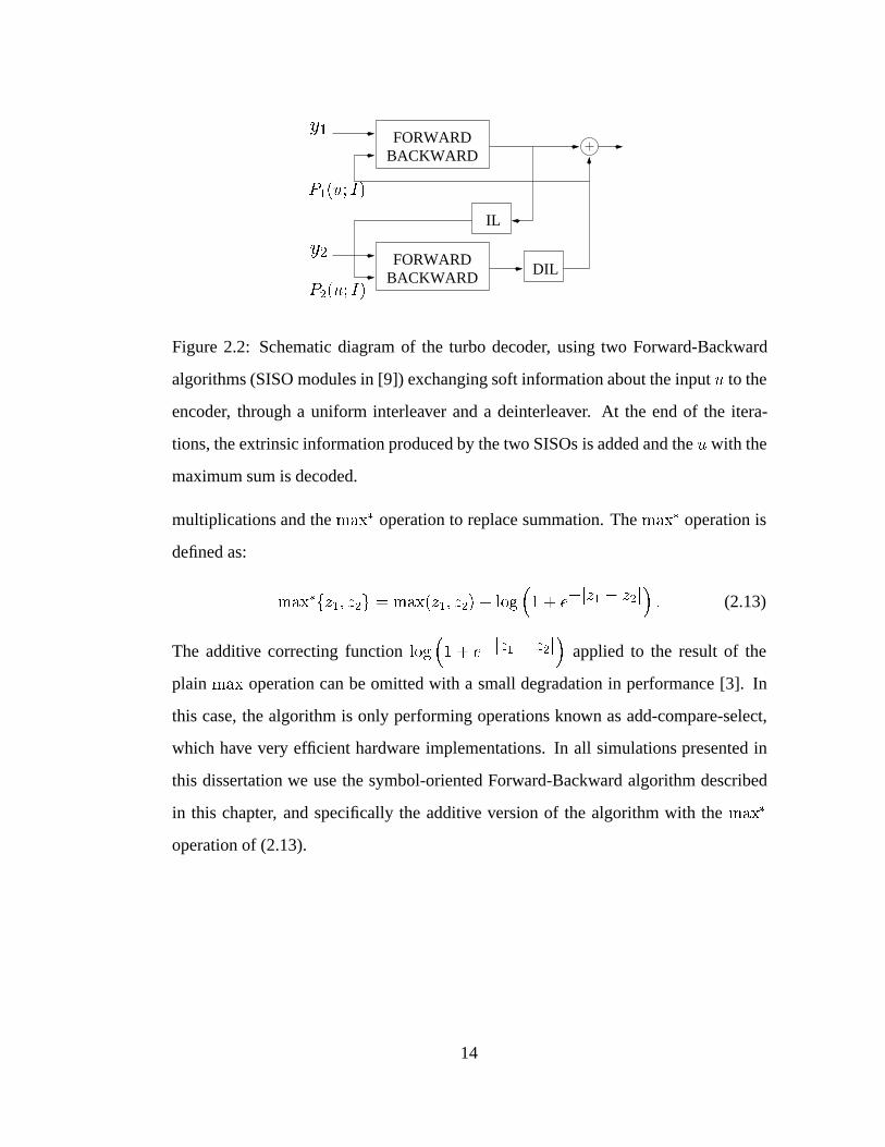
FORWARDBACKWARD
FORWARDBACKWARD DIL
IL
P1(u; I)
P2(u; I)
y2
y1
Figure 2.2: Schematic diagram of the turbo decoder, using two Forward-Backward
algorithms (SISO modules in [9]) exchanging soft information about the input u to the
encoder, through a uniform interleaver and a deinterleaver. At the end of the itera-
tions, the extrinsic information produced by the two SISOs is added and the u with the
maximum sum is decoded.
multiplications and the max� operation to replace summation. The max� operation is
defined as:
max�fz1; z2g = max(z1; z2) + log�1 + e
�jz1 � z2j�: (2.13)
The additive correcting function log�1 + e
�jz1 � z2j�
applied to the result of the
plain max operation can be omitted with a small degradation in performance [3]. In
this case, the algorithm is only performing operations known as add-compare-select,
which have very efficient hardware implementations. In all simulations presented in
this dissertation we use the symbol-oriented Forward-Backward algorithm described
in this chapter, and specifically the additive version of the algorithm with the max�
operation of (2.13).
14
CHAPTER 3
Flat Rayleigh Fading
A widely accepted statistical model for non-dispersive wireless fading channels has
been introduced in [15], and is commonly referred to as Clarke’s fading model. Ac-
cording to this model, after matched filtering and proper sampling, the discrete repre-
sentation of the received signal at time t is:
yt = at � xt + nt; t = 0; 1; 2; : : : (3.1)
where xt is the transmitted constellation point (in this chapter from an M -PSK con-
stellation), fntg is an i.i.d. (white) complex Gaussian noise process, with variance
�2 = No=2 per dimension, and fatg is the correlated channel fading process, mod-
eled as a circular complex Gaussian random process. This model assumes absence of
line of sight (worst case fading) and a continuum of scatterers in the vicinity of the
omnidirectional mobile receiver antenna, in other words a rich scattering environment.
Under those conditions, the channel coefficient at time t is at = Xt + jYt =
jatjej�at , where fXtg and fYtg are mutually uncorrelated, zero-mean Gaussian pro-
cesses, each with correlation properties determined by the Doppler frequency fD, see
[16]:
Rc(�) = E[XtXt+� ] = E[YtYt+� ] = 2Jo(2�fD�) (3.2)
where Jo(�) is the zero-order modified Bessel function of the first kind, and 2 = 0:5
for normalized power. This autocorrelation gives rise to the well-known U-shaped
15
normalized power spectral density in Jakes [17]:
Sxx(f) = Syy(f) =
8>>>><>>>>:1
2�fDT
1s1�
�f
fDT
�2; jf j < fDT
0; otherwise
(3.3)
If fXtg and fYtg are zero-mean (worst case—no line of sight), the marginal distribu-
tions of jatj and �at are Rayleigh and uniform respectively, hence the term “Rayleigh
fading”. Specifically, the marginal pdf of the phase is P�a(�) = 1=2�, for � 2 [��; �),while the amplitude marginal pdf for normalized unit power is Pjaj(r) = 2r e�r
2
, for
r � 0.
3.1 Markov model for the phase
Clarke’s model for the channel fading process is realistic and has been found to quite
accurately match field measurements of physical channels. However, the autocor-
relation properties of the amplitude process fjatjg and, mainly, the phase process
f�at g, which poses the primary problem in PSK transmission, are non-Markovian and
hence difficult to analyze and exploit with the Forward-Backward algorithm. Based on
the spectrum of (3.3), the correlation coefficient �jaj(�) for the fading amplitude and
��a(�) for the phase of the fading process fatg are shown in Fig. 3.1. Observe that the
autocorrelation is decreasing with the time-lag, as expected, but not in an exponential
fashion, as in a truly Markov process.
To utilize the power of the Forward-Backward algorithm in estimation we derive
a suitable finite-state Markov model for the channel phase, depending on the Doppler
rate fDT , similar to the one in [18] for the fading amplitude. The issue of whether
approximating Clarke’s fading process [17] with a first-order Markov process is rea-
sonable or not was answered in the affirmative in [19] for the fading amplitude, but the
16
0 5 10 15 20 25 30 35 40−0.25
0
0.25
0.5
0.75
1
1.25
�=T , lag (in samples)
�jaj(�)��a(�)
Figure 3.1: Correlation coefficient for the amplitude and the phase of the fading pro-
cess fatg for fDT = 0:05. The approximation used in [16] to derive ��a(�) for the
phase is problematic at small lags, hence the dotted part of the curve.
result also carries over to the channel phase process, which is of interest here. Specifi-
cally, for the amplitude fading rt = jatj of a phase-coherent channel it is shown in [19]
that the ratio I(rt; rt�2j rt�1)=I(rt; rt�1; rt�2), which is a measure of deviation from
Markovity for the channel amplitude frtg, is very small, and becomes smaller with
decreasing Doppler rate. A similar result can be shown for the fading phase process
f�at g. Besides, it is intuitively obvious that a Markov model with a sufficiently high
number of states can mimic the statistics of any process arbitrarily well, although the
number of states necessary in our case to make the model very accurate would be be-
17
yond practical interest. In this dissertation, we limit the number of states K to a small
integer multiple of the cardinality of the PSK constellation for simplicity.
The receiver can form a K-state Markov model for the quantized version Qt of
the phase fading process �at , where fQtg; t = 0; 1; 2; : : : is a time-homogeneous,
discrete-time, stationary Markov chain, taking values in the finite state space Q =
fq0; q1; : : : ; qK�1g, a set of “quantized channel phase distortion states” qi:
qi =2�i
K
; i = 0; 1; 2; : : : ; K � 1; (3.4)
in the following fashion, introducing a quantization operator �(:):
Qt = qi , �(�at ) = qi , �at 2
hqi � �
K
; qi +�
K
�:
The transition probabilities Pqi;qj , i; j = 0; 1; : : : ; K � 1 of the Markov chain are
independent of t by stationarity, and can be computed for known Doppler rate fDT
from the joint pdf of two successive sampled fading phases:
Pqi;qj = Pr(Qt+1 = qj j Qt = qi) (3.5)
=
R qi+�=Kqi��=K
R qj+�=Kqj��=K
p(�at ; �at+1)d�
at d�
at+1R qi+�=K
qi��=Kp(�at )d�
at
(3.6)
where the marginal pdf is uniform, and the joint pdf is [16]:
p(�at ; �at+1)=
1� �2
4�2
�p1� B
2 +B(� � B cos�1(B))
(1� B2)3=2
�where B = � � cos(�at+1 � �
at ), and � = Jo(2�fDT ).
The model described above is essentially an approximation in a dual sense: First, it
maps all real fading angles �a 2 [��; �) to a finite number of “quantized fading phase
states” qi, i = 0; 1; : : : ; K � 1. Moreover, the model approximates the dynamics of
the continuous process f�at gt=0;1;::: ;1 with a discrete Markov chain, taking values in
the finite-state space Q and having stationary probabilities pi = 1=K and transition
18
probabilities Pqi;qj . It should be noted, however, that the channel estimation algorithm
(based on the Forward-Backward algorithm) in Rayleigh fading does not perceive the
channel phase as quantized to the K values of (3.4); the algorithms of Chapters 4 and
5 remain aware of the continuous nature of �at , but are based on the assumption that
�at is uniformly distributed in a sector of length 2�=K, given that it belongs in that
sector. Hence, the finite-state Markov model is merely a way to reduce the infinite
cardinality of the set of possible phases �at to K “phase states”, such that reliabilities
can be assigned to them by the Forward-Backward algorithm.
4 4.5 5 5.5 6 6.5 710
−5
10−4
10−3
10−2
10−1
fDT = 0:01, 10sy.-1pi.
fDT = 0:05, 5sy.-1pi.
Es=No, in dB
BE
R
cjatj = Ajytj + B
Genie-provided jatj
Figure 3.2: BER of turbo-code, in different fDT , for different pilot insertion ratios.
Performance with affine fading amplitude estimation from the received amplitude is
very close to the case when the receiver has access to genie-provided channel ampli-
tude jatj.
A Markov model closely related to the one described above was derived in [18]
to model the amplitude fading of a phase-coherent Rayleigh fading channel. In that
19
paper, several channel amplitude levels corresponded to binary symmetric channels
(BSCs) with different crossover probabilities, thereby creating a Finite-State Markov
Channel (FSMC). Here we recognize the phase distortion in a Rayleigh channel as a
more severe problem for PSK transmission than amplitude fading.
This qualitative observation, along with the difficulty of obtaining coherent phase
reference in a high Doppler, low SNR environment, indicates that the main channel
estimation effort for PSK turbo-codes should be devoted to acquiring phase coherence
rather than exact estimates for the fading amplitude jatj. Thus, the two receivers de-
rived in the next chapter create the finite-state Markov (FSM) model outlined above
and use it to estimate the channel phase with the Forward-Backward algorithm [12].
For the fading amplitude estimation they rely on a simple MMSE, symbol-by-symbol
affine estimator from the received amplitude of the form cjatj = Ajytj + B. As shown
in Fig. 3.2, this method for amplitude estimation, combined with Forward-Backward
phase estimation on the FSM phase model, performs only slightly worse than when
having perfect channel amplitude knowledge at the receiver. This result supports the
decision to use a simple estimator for the fading amplitude and reserve the power of
the Forward-Backward algorithm for phase estimation.
3.2 Quantized phase estimation
The performance of turbo-codes in flat fading was examined in [4]. In [20] and [21] it
was recognized that additional performance benefits are possible when moving from
“one-shot” channel estimation (e.g. from pilots) to iterative estimation, integrated with
turbo decoding. Specifically, in [20] and [21] the channel estimators perform optimum
(Wiener) filtering of symbols at each iteration (only pilots at first, and all symbols
in subsequent iterations taking into account their reliability), thus exploiting extrinsic
information produced by the turbo decoder about coded symbols.
20
In this section, we also apply the principle of iterative channel estimation, but not
with filtering of pilots and coded symbols. Instead, we employ the Forward-Backward
algorithm for “quantized phase” estimation based on the FSM model derived in sec-
tion 3.1. In section 4.1.1 joint phase estimation and turbo decoding proceed along a
supertrellis, constructed by merging the trellises of the code and the Markovian chan-
nel state structure. In section 4.1.2 we demonstrate better performance by using a
separate Forward-Backward algorithm to estimate the phase state, operating on the
trellis of the FSM phase model and exchanging soft information with the constituent
decoder SISO [9].
Notice that in both approaches the Forward-Backward algorithm operates on the
K-state Markov phase model, and obtains soft phase estimates in the form of a proba-
bility distribution on the K phase states at each time instant (implicitly in the supertrel-
lis, explicitly with the separate trellises). Fig. 3.3 demonstrates the rationale behind this
choice of “quantized phase” estimation: at the low SNR where turbo-codes operate, it
is advantageous to have a phase estimate with small precision but high reliability (as
is possible with the Forward-Backward algorithm on a finite-state phase model) rather
than continuous valued estimates of limited reliability, like those provided by optimum
filtering, which exhibits higher MSE.
Under the assumption of knowing the correct phase state (i.e. sector), which is a
reasonable assumption with the Forward-Backward algorithm, Fig. 3.3 indicates that
at low SNR and high Doppler (or, equivalently more sparse pilot spacing under the
chosen Doppler of fDT = 0:05) the “quantized phase” estimation approach outper-
forms Wiener filtering solutions in the estimation MSE sense, even with the coarse,
symbol-by-symbol amplitude estimation cjatj = Ajytj+B. In fact, it is this amplitude
error that accounts for most of the estimation MSE, as seen from the fact that beyond
K = 32 no additional MSE gain is obtained by increasing the number of “quantized
21
phase states.” Of course, at high SNR optimum linear pilot filtering works better than
our non-linear “quantized phase” estimation, even if this is assumed to always identify
the correct sector.
However, “quantized” estimation seems to have an advantage in the very noisy
region of operation of turbo-codes, insofar as the channel estimation MSE is an indi-
cation of turbo-code bit error rate performance. For a fixed SNR, the sequence of thin
curves shows decreasing MSE from linear filtering for increasing pilot density. This
can be thought of as the improvement to channel estimation expected as the Wiener
filter acquires more knowledge about the transmitted data through the turbo iterations.
Even in this case, (e.g. when every third symbol becomes perfectly known, i.e. D = 2,
the lowest thin curve in Fig. 3.3) if the non-linear phase estimation guesses the correct
sector it promises slightly less MSE at low SNR.
For the derivation of the MSE in the cases of D > 0, please refer to Appendix A.
The dotted curve, corresponding to the MSE of estimation when all coded symbols are
known (essentially forD = 0, or estimation of ak from all observables yt = at+nt; t =
�1; : : : ;1) is only included in the plot to mark the best estimation MSE that could
be hoped for, if all data symbols were known. Of course, in that case there would
be no need for decoding, and thus no need for channel estimation either. It comes
as no surprise that this scenario (all symbols known) induces the lowest estimation
MSE. The analytical expression for it is derived from a well-known result for optimal
discrete-time smoothing (see, for instance, [22]).
Given all observations yt; t = �1; : : : ;1 of a process fytg, the optimum (i.e. lin-
ear least-mean-square) l.l.m.s. estimator of the process fatg is the so-called non-causal
Wiener filter:
K
�ej!�=Say(e
j!)
Sy(ej!); (3.7)
22
and the corresponding minimum mean-squared error (m.m.s.e) is:
Ej~atj2 = 1
2�
Z �
��
�Sa
�ej!�� jSay(ej!) j2
Sy(ej!)d!
�(3.8)
In our case, the noise is additive (yt = at + nt) with power spectral density Sn(f) =
No = �2n, so the power spectra involved in the m.m.s.e. are:
Say(f) = Sa(f) =1
�
pf2d � f
2; jf j � fd; (3.9)
Sy(f) = Sa(f) + Sn(f) = Sa(f) +No; (3.10)
where fd = fDT is the discrete Doppler frequency.
So, the m.m.s.e. becomes (with f = !=2�):
m.m.s.e. =
Z 1=2
�1=2
No � Sa(f)No + Sa(f)
df (3.11)
= No �Z fd
�fd
1
1 +No�
pf2d � f
2df (3.12)
=2
�
� �
2+
2�p1� �
2� arctanh
� � 1p1� �
2
!!; (3.13)
where � =1
��2nfd
=1
�NofDT. Observe the synergistic effect of increasing Doppler
rate and noise power in the expression for the m.m.s.e., which indicates that the es-
timation task becomes increasingly difficult for a more-noisy, faster-varying channel.
Conversely, for fDT ! 0 (no variation) and/or �n ! 0 (no noise) the estimation
MSE with an optimum smoothing filter of infinite length goes to zero, as expected
intuitively.
23
0 5 10 150
0.05
0.1
0.15
0.2
0.25
0.3
0.35
0.4
0.45
0.5Averaging 10 pilots Averaging 20 pilots Averaging 40 pilots proposed method, K=8, 16, 32all symbols known, D=0
Es=No, in dB
MSE
D = 8
D = 4
D = 2
Figure 3.3: Mean-Squared Error (MSE) of channel estimation for a Rayleigh fading
channel with fDT = 0:05 under two scenarios: thin lines represent MSE after Wiener
filtering of 10, 20, or 40 pilot symbols spaced one every D data symbols, while thick
lines show the MSE resulting from simple affine amplitude estimation using only the
received amplitude, and uniform phase uncertainty within a sector of 2�=K radians,
K = 8; 16; 32, given that the correct sector is known. Note that this largely corre-
sponds to the estimation procedure followed in the sequel. Observe that for low SNR
the second approach is better. Of course, the dotted thin curve of the MSE when all
symbols are known (could be thought of as “D = 0”) is the best of all, but this serves
only as an indication of the lowest MSE that can be hoped for.
24
CHAPTER 4
Algorithms for Joint Data and Channel Estimation
Optimal decoding in flat fading —either minimum bit error rate (MAP) decoding or
maximum likelihood sequence detection (MLSD)— requires either explicit or implicit
estimation of the channel. This chapter describes the FSM-model-based receiver algo-
rithms in detail and presents simulation results.
4.1 Forward-Backward phase estimation
For “quantized phase” estimation with the Forward-Backward algorithm either on a
supertrellis or on separate trellises the basic quantities needed are the probabilities
Pq0;q of the channel phase transitioning from state (sector) q0 to q (given in (3.5)-(3.6))
and the likelihoods P (yt j Qt = q; xt = x). At time t, the received complex symbol is
yt = jytj � ej�yt , where the total received angle �yt is the sum of three distinct angles:
�
yt = �
xt + �
at + �
�t ; (4.1)
as shown in Fig. 4.1. In this figure, �xt is the transmitted constellation point angle,
as the constituent trellis M-PSK code transitions from state c0 to c, i.e., xt(c0 ! c) =
1 � ej�xt . The fading angle �at is defined from the fading scale factor at = jatj � ej�at , and
��t is the noise-induced additional angle, having distribution P (��):
P (��;�) =e��2
2��h1 +
p�� cos��e(� cos �
�)2erfc(�� cos��)i; (4.2)
25
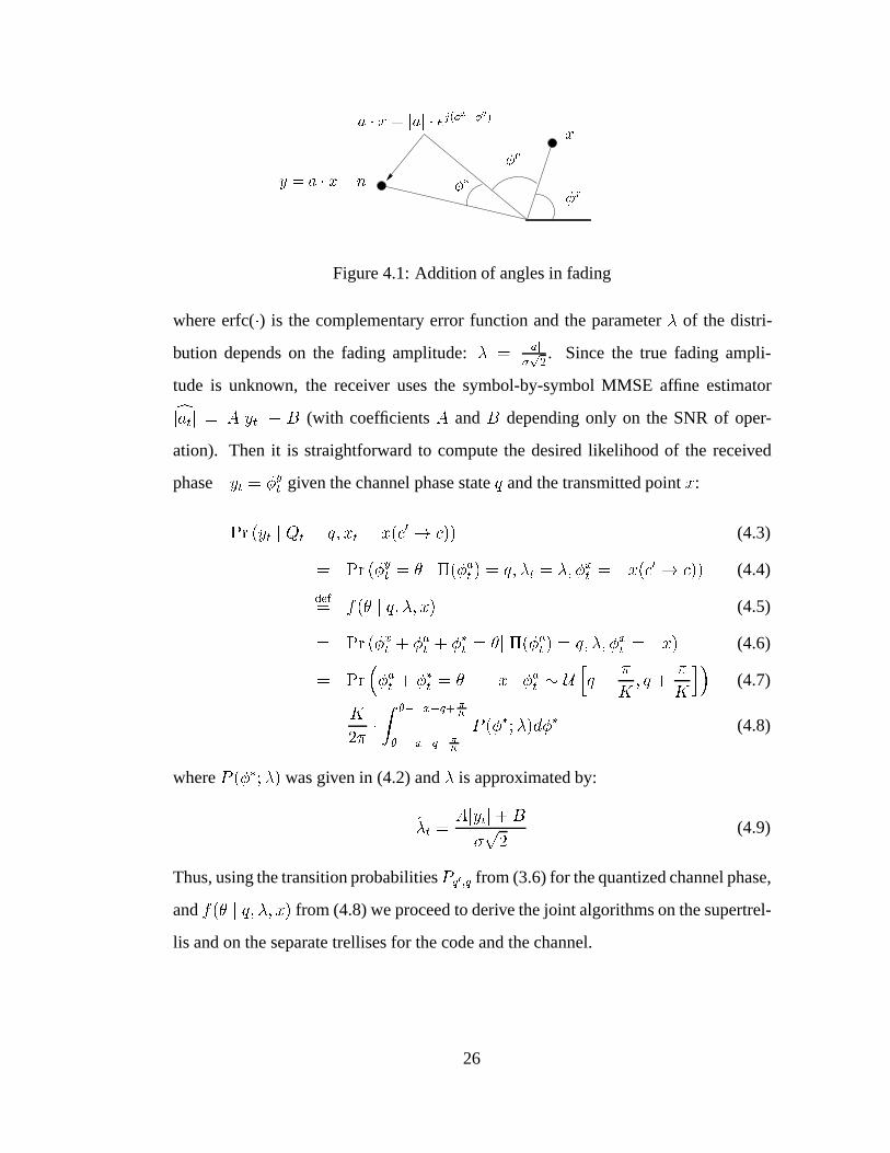
y = a � x + n
xa � x = jaj � ej(�
x+�a)
��
�x
�a
Figure 4.1: Addition of angles in fading
where erfc(�) is the complementary error function and the parameter � of the distri-
bution depends on the fading amplitude: � =jaj�p2. Since the true fading ampli-
tude is unknown, the receiver uses the symbol-by-symbol MMSE affine estimatorcjatj = Ajytj + B (with coefficients A and B depending only on the SNR of oper-
ation). Then it is straightforward to compute the desired likelihood of the received
phase \yt = �
yt given the channel phase state q and the transmitted point x:
Pr (yt j Qt = q; xt = x(c0 ! c)) = (4.3)
= Pr (�yt = � j �(�at ) = q; �t = �; �
xt = \x(c
0 ! c)) (4.4)
def= f(� j q; �; x) (4.5)
= Pr (�xt + �at + �
�t = �j �(�at ) = q; �; �
xt = \x) (4.6)
= Pr��at + �
�t = � � \x j �at � U
hq � �
K
; q +�
K
i�(4.7)
=K
2��Z ��\x�q+ �
K
��\x�q� �
K
P (��;�)d�� (4.8)
where P (��;�) was given in (4.2) and � is approximated by:
�t =Ajytj+B
�
p2
(4.9)
Thus, using the transition probabilitiesPq0;q from (3.6) for the quantized channel phase,
and f(� j q; �; x) from (4.8) we proceed to derive the joint algorithms on the supertrel-
lis and on the separate trellises for the code and the channel.
26
4.1.1 Supertrellis algorithm
An initial approach to joint estimation and decoding is to combine the Markov model
for the quantized fading phase discussed in Chapter 3 with the trellis describing the
code, to form a supertrellis. In essence, the receiver observes the output of a finite-
state machine (i.e., the encoder output xt) multiplied with the output of a Markov
process (i.e., the “fading phase state” Qt) under AWGN. At time t, the state St of the
supertrellis is an ordered pair consisting of the channel state Qt and the code state Ct,
giving St = (Qt; Ct) = (q; c) = m, with m = 0; 1; : : : ; 2�K � 1, for a code with �
memory elements.
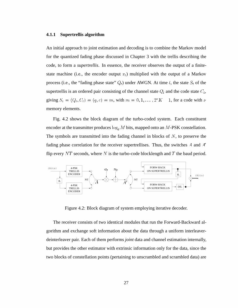
Fig. 4.2 shows the block diagram of the turbo-coded system. Each constituent
encoder at the transmitter produces log2M bits, mapped onto anM -PSK constellation.
The symbols are transmitted into the fading channel in blocks of N , to preserve the
fading phase correlation for the receiver supertrellises. Thus, the switches A and A0
flip every NT seconds, where N is the turbo-code blocklength and T the baud period.
ON SUPERTRELLISFORW-BACK
ON SUPERTRELLISFORW-BACK
IL
DIL
IL
TRELLISENCODER
4-PSK
TRELLISENCODER
4-PSK{Bits}
NT
{Bits}
NT
ntat
A A0
Figure 4.2: Block diagram of system employing iterative decoder.
The receiver consists of two identical modules that run the Forward-Backward al-
gorithm and exchange soft information about the data through a uniform interleaver-
deinterleaver pair. Each of them performs joint data and channel estimation internally,
but provides the other estimator with extrinsic information only for the data, since the
two blocks of constellation points (pertaining to unscrambled and scrambled data) are
27
transmitted successively into the channel and undergo independent fading. Thus, in-
formation about the channel produced by one of the estimators would be irrelevant to
the other. However, within each block of N symbols, the channel is correlated, which
facilitates the joint estimation of channel phase and data.
The crucial quantity to compute in each supertrellis for iterative decoding [9], is:
t(m0; m)
def= Pr (yt; St = (q; c) j St�1 = (q0; c0)) = (4.10)
= Pr (St = (q; c)jSt�1 = (q0; c0)) � Pr (yt jSt�1 = (q0; c0); St = (q; c)) (4.11)
For the first term of (4.11) we have:
Pr (St = (q; c) j St�1 = (q0; c0)) =
= Pr��(�at ) = q j�(�at�1) = q
0� � Pr (ut such that Ct = c jCt�1 = c0) (4.12)
= Pq0;q � P (ut; I); (4.13)
where P (ut; I) denotes the extrinsic information about the input ut provided by the
other soft decoder, and Pq0;q is the transition probability (3.5) of the quantized channel
phases. The second term of (4.11) is clearly f(� j q; �; x) as defined in (4.5)-(4.8).
Note that the algorithm described above can be used with or without pilot symbols.
The transition metric t(m0; m) of (4.10) connects only superstates (m0
; m) with valid
code state transitions (c0 ! c). In the case of pilots injected in the coded data stream,
the code state does not change, and the only valid supertrellis branches are those with
c = c0. Here we only present simulation results with no pilot symbols.
Fig. 4.3 presents the simulated BER performance of the system depicted in Fig. 4.2
under Rayleigh fading with fDT = 0:05. The constituent codes are identical, 8-state,
recursive systematic rate-1/2, Gray-labeled 4-PSK codes, with maximum effective
Hamming distance. They are fully described by the octal parity polynomials h0 = 15
and h1 = 17. The number of quantized phases was K = 8, resulting in 64-state
28
0 2 4 6 8 10 1210
−5
10−4
10−3
10−2
10−1
iterative joint estimator, correl. Rayleighsame turbo−code, i.i.d. Rayleigh, perf. CSIsame turbo−code, correl. Rayleigh, pilots
Eb=N
o, in dB
BE
R
C
Figure 4.3: Supertrellis and non-iterative pilot filtering performance in Clarke’s chan-
nel with fDT = 0:05. The dashed curve shows performance of the same turbo-code in
the same channel with ideal interleaving and perfect CSI at the receiver. The dashed
vertical line marks the capacity in this ideal case.
supertrellises, and the blocklength was N = 5000 symbols. For this relatively high
Doppler rate the performance is about 6:5 dB worse than when the same turbo-code
operates under the ideal assumptions of perfect interleaving and perfect CSI (dashed
curve). However, this gap is not very informative, since the constrained capacity of the
two channels considered with uniform i.i.d. 4-PSK inputs is quite different at this high
Doppler.
The vertical dashed line (“C” in Fig. 4.3) marks the capacity of the idealized sce-
nario of perfectly known at at receiver. It is simply I(X;Y jA), a weighted aver-
age of the AWGN capacity under the Rayleigh distribution pA(a) = 2a e�a2
, giving
29
Eb=No = �0:08 dB for the rate 1=2 of interest. The capacity is smaller when CSI is un-
available at the receiver and has to be estimated from received values (much smaller for
larger Doppler rates, and zero in the limit of i.i.d. fading). A more detailed discussion
about constrained 4-PSK capacity under fading follows in section 4.2.2. To demon-
strate the difficulty of obtaining accurate CSI in a practical system at high Doppler, we
also simulated a pilot-symbol assisted system [23] with the same turbo-code. Specif-
ically, a more sophisticated variant of pilot averaging in [24], using 3 pilot symbols
every 5 data symbols performs almost 4 dB worse than our joint iterative estimator
with no pilot symbols at all. Even if we plot against Es=No disregarding the sacrifice
of 3=8 = 37:5% in rate of the pilot system [24], the supertrellis system is still almost
2 dB better. The reason is that essentially every coded symbol with the supertrellis
iterations becomes somewhat a pilot, as its reliability increases.
The supertrellis receiver designed and simulated in this section has advantages and
limitations. An obvious advantage is its ability to work without external acquisition
circuitry or pilot symbols at relatively high Doppler rate. The low rate of each con-
stituent code (here 1=2) compensates for the absence of pilot symbols, allowing the
supertrellis algorithm to determine whether a change in the received phase is due to
the code or to a change in the channel. Thus, although this scheme does not lose rate
directly because of pilots that bear no information, it is the rate reduction inherent in
the constituent encoder design that makes channel estimation possible. On a higher
level this can be viewed as incorporating the training in the code design, instead of
explicitly injecting pilot symbols in the coded data stream of a higher rate code.
The main limitation is computational complexity, since the number of states in
each supertrellis is the product of the code states and the number of phase intervals
K. If M -PSK is used, then K � 2 �M for reasonable phase estimation. This leads
to at least 64-state supertrellises with 4-PSK and 128-states with 8-PSK for 8-state
30
constituent codes. Another limitation concerns diversity. The channel estimation pro-
cedure along the supertrellis precludes channel interleaving, because the algorithm
relies on the correlation between successive phases. Hence, only implicit diversity,
due to the interleaver between constituent codes, is provided.
4.1.2 Algorithm on separate trellises
In this section we derive and simulate a better structure for joint channel estimation and
turbo decoding based on the Forward-Backward algorithm running on separate trellises
for the channel phase and the code. Unlike the supertrellis algorithm presented in sec-
tion 4.1.1, the joint iterative receiver in this section relies on known pilot symbols [23]
for initial and subsequent channel estimates. For a powerful high-rate channel code,
we designed a trellis turbo-code with overall rate of 1 bit/sec/Hz, where the constituent
encoders are the best 8-state, rate-2/2 code fragments (see [5]-[10]), each producing
one systematic and one parity bit per 2-bit input, and their outputs are mapped onto a
Gray-labeled 4-PSK constellation, as shown in Fig. 4.4. This turbo-code will be the
running example in this section and in the next chapter.
Observe that the trellis turbo encoder depicted in Fig. 4.4 is similar to the generic
form discussed in Chapter 2 and [10]. Despite the difference in generating the parity
bits, the encoder in Fig. 4.4 can be shown to be exactly equivalent to the generic form
in Fig. 2.1 of Chapter 2. The specific constituent encoders, described by the set of octal
polynomials fh0 = 13; h1 = 7; h2 = 1; h3 = 17g, corresponding to the feedback, the
entrance of the two input bits, and the generation of the output bit respectively were
identified by exhaustive search conducted as in [10]. The interested reader can find
more details about constituent encoder design for trellis turbo-codes in [6] and [7].
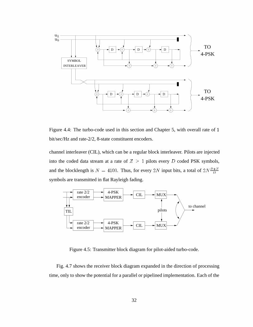
Fig. 4.5 shows the transmitter block diagram. Notice the difference between the
turbo interleaver (TIL), which is a random interleaver obtained as in [6, Ch. 4], and the
31
D D D
D D D
SYMBOL
INTERLEAVER
u1u0
TO4-PSK
TO4-PSK
Figure 4.4: The turbo-code used in this section and Chapter 5, with overall rate of 1
bit/sec/Hz and rate-2/2, 8-state constituent encoders.
channel interleaver (CIL), which can be a regular block interleaver. Pilots are injected
into the coded data stream at a rate of Z � 1 pilots every D coded PSK symbols,
and the blocklength is N = 4100. Thus, for every 2N input bits, a total of 2N D+ZD
symbols are transmitted in flat Rayleigh fading.
rate 2/2encoder
4-PSKMAPPER
MUX
rate 2/2encoder
4-PSKMAPPER
MUX
TIL
CIL
CIL
pilotsto channel
Figure 4.5: Transmitter block diagram for pilot-aided turbo-code.
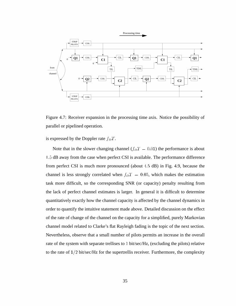
Fig. 4.7 shows the receiver block diagram expanded in the direction of processing
time, only to show the potential for a parallel or pipelined implementation. Each of the
32
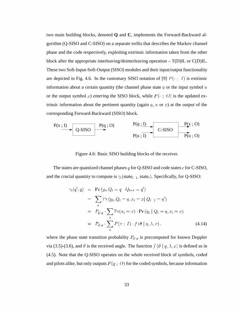
two main building blocks, denoted Q and C, implements the Forward-Backward al-
gorithm (Q-SISO and C-SISO) on a separate trellis that describes the Markov channel
phase and the code respectively, exploiting extrinsic information taken from the other
block after the appropriate interleaving/deinterleaving operation – T(D)IL or C(D)IL.
These two Soft-Input-Soft-Output (SISO) modules and their input/output functionality
are depicted in Fig. 4.6. In the customary SISO notation of [9] P (� ; I) is extrinsic
information about a certain quantity (the channel phase state q or the input symbol u
or the output symbol x) entering the SISO block, while P (� ; O) is the updated ex-
trinsic information about the pertinent quantity (again q, u or x) at the output of the
corresponding Forward-Backward (SISO) block.
Q-SISOP(x ; I) P(q ; O)
C-SISOP(q ; I)
P(u ; I)
P(x ; O)
P(u ; O)
Figure 4.6: Basic SISO building blocks of the receiver.
The states are quantized channel phases q for Q-SISO and code states c for C-SISO,
and the crucial quantity to compute is t(statet�1; statet). Specifically, for Q-SISO:
t(q0; q) = Pr (yt; Qt = q j Qt�1 = q
0)
=Xx
Pr (yt; Qt = q; xt = xj Qt�1 = q0)
= Pq0;q �Xx
Pr(xt = x) � Pr (yt j Qt = q; xt = x)
= Pq0;q �Xx
P (x ; I) � f (� j q; �; x) ; (4.14)
where the phase state transition probability Pq0;q is precomputed for known Doppler
via (3.5)-(3.6), and � is the received angle. The function f (� j q; �; x) is defined as in
(4.5). Note that the Q-SISO operates on the whole received block of symbols, coded
and pilots alike, but only outputsP (q ; O) for the coded symbols, because information
33
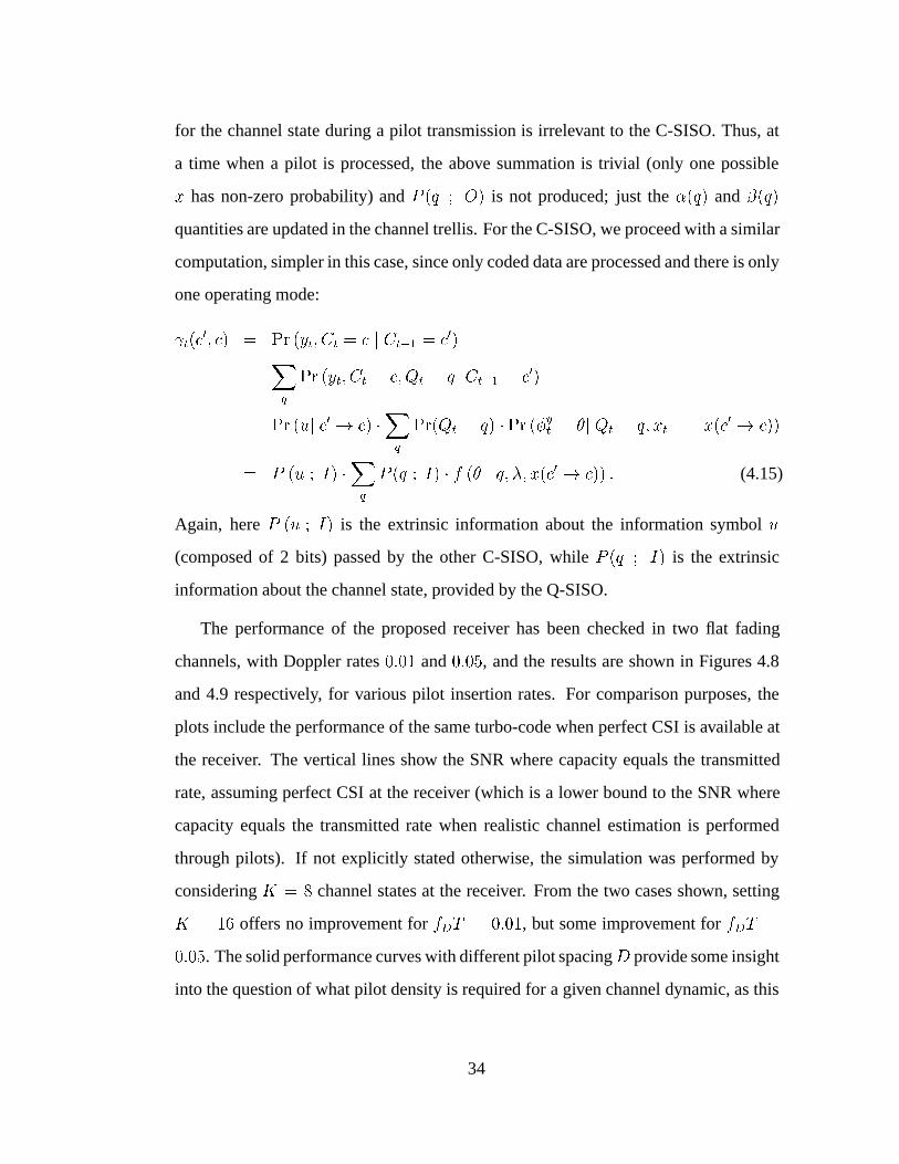
for the channel state during a pilot transmission is irrelevant to the C-SISO. Thus, at
a time when a pilot is processed, the above summation is trivial (only one possible
x has non-zero probability) and P (q ; O) is not produced; just the �(q) and �(q)
quantities are updated in the channel trellis. For the C-SISO, we proceed with a similar
computation, simpler in this case, since only coded data are processed and there is only
one operating mode:
t(c0; c) = Pr (yt; Ct = c j Ct�1 = c
0)
=Xq
Pr (yt; Ct = c; Qt = qj Ct�1 = c0)
= Pr (uj c0 ! c) �Xq
Pr(Qt = q) � Pr (�yt = �j Qt = q; xt = \x(c0 ! c))
= P (u ; I) �Xq
P (q ; I) � f (� j q; �; x(c0 ! c)) : (4.15)
Again, here P (u ; I) is the extrinsic information about the information symbol u
(composed of 2 bits) passed by the other C-SISO, while P (q ; I) is the extrinsic
information about the channel state, provided by the Q-SISO.
The performance of the proposed receiver has been checked in two flat fading
channels, with Doppler rates 0:01 and 0:05, and the results are shown in Figures 4.8
and 4.9 respectively, for various pilot insertion rates. For comparison purposes, the
plots include the performance of the same turbo-code when perfect CSI is available at
the receiver. The vertical lines show the SNR where capacity equals the transmitted
rate, assuming perfect CSI at the receiver (which is a lower bound to the SNR where
capacity equals the transmitted rate when realistic channel estimation is performed
through pilots). If not explicitly stated otherwise, the simulation was performed by
considering K = 8 channel states at the receiver. From the two cases shown, setting
K = 16 offers no improvement for fDT = 0:01, but some improvement for fDT =
0:05. The solid performance curves with different pilot spacingD provide some insight
into the question of what pilot density is required for a given channel dynamic, as this
34
Q1
TIL TIL
PILOTSSTRIP
PILOTSSTRIP
CDIL
CDIL
CDIL
CDIL
CDIL
CILCDIL
CIL
CIL
CIL
TDIL TDIL
Q1 C1
Q2 C2
Q1
Q2 C2
C1
0
0
0
Processing time
from
channel
Figure 4.7: Receiver expansion in the processing time axis. Notice the possibility of
parallel or pipelined operation.
is expressed by the Doppler rate fDT .
Note that in the slower changing channel (fDT = 0:01) the performance is about
1:5 dB away from the case when perfect CSI is available. The performance difference
from perfect CSI is much more pronounced (about 4:5 dB) in Fig. 4.9, because the
channel is less strongly correlated when fDT = 0:05, which makes the estimation
task more difficult, so the corresponding SNR (or capacity) penalty resulting from
the lack of perfect channel estimates is larger. In general it is difficult to determine
quantitatively exactly how the channel capacity is affected by the channel dynamics in
order to quantify the intuitive statement made above. Detailed discussion on the effect
of the rate of change of the channel on the capacity for a simplified, purely Markovian
channel model related to Clarke’s flat Rayleigh fading is the topic of the next section.
Nevertheless, observe that a small number of pilots permits an increase in the overall
rate of the system with separate trellises to 1 bit/sec/Hz, (excluding the pilots) relative
to the rate of 1=2 bit/sec/Hz for the supertrellis receiver. Furthermore, the complexity
35
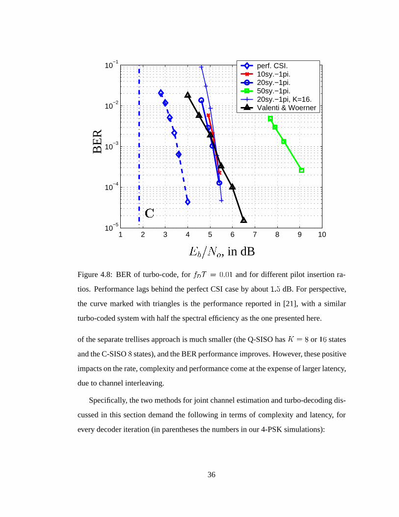
1 2 3 4 5 6 7 8 9 1010
−5
10−4
10−3
10−2
10−1
perf. CSI. 10sy.−1pi. 20sy.−1pi. 50sy.−1pi. 20sy.−1pi, K=16. Valenti & Woerner
BE
R
C
Eb=N
o, in dB
Figure 4.8: BER of turbo-code, for fDT = 0:01 and for different pilot insertion ra-
tios. Performance lags behind the perfect CSI case by about 1:5 dB. For perspective,
the curve marked with triangles is the performance reported in [21], with a similar
turbo-coded system with half the spectral efficiency as the one presented here.
of the separate trellises approach is much smaller (the Q-SISO has K = 8 or 16 states
and the C-SISO 8 states), and the BER performance improves. However, these positive
impacts on the rate, complexity and performance come at the expense of larger latency,
due to channel interleaving.
Specifically, the two methods for joint channel estimation and turbo-decoding dis-
cussed in this section demand the following in terms of complexity and latency, for
every decoder iteration (in parentheses the numbers in our 4-PSK simulations):
36

1 2 3 4 5 6 7 8 9 10
10−5
10−4
10−3
10−2
10−1 perf. CSI.
1sy.−1pi. 5sy.−1pi. 5sy.−3pi. 10sy.−1pi. 5sy.−1pi, K=16.
BE
R
C
Eb=N
o, in dB
Figure 4.9: BER of turbo-code, for fDT = 0:05 and for different pilot insertion ratios.
� supertrellis: two Forward-Backward algorithms, each on a supertrellis with 2� �K states (64 states), and 2K branches (16 here) emanating from each state. This
number can be reduced, by pruning less likely transitions to phase-states far
apart from the current one, particularly for small Doppler rates. This receiver
suffers no extra latency from channel interleaving.
� separate trellises: less complexity, four Forward-Backward algorithms in all.
Two for the two fully connected K-state Q-SISOs (K = 8), and two for the
2�-state C-SISOs (� = 3). Higher latency, because of channel interleaving at
the transmitter and deinterleaving at the receiver. Here we implemented those
block interleavers to be of equal size to the turbo-code blocklength N , but this
37
is not necessary, particularly for high Doppler rates. The turbo-code latency is
obviously unavoidable.
Finally, for comparison, the complexity of a pilot-averaging system obtaining one-
shot channel estimates without iteration is just two 2�-state C-SISOs per iteration, plus
the additional one-time cost of pilot filtering per block. The latency from channel
interleaving is the same as in the separate trellises scenario. Thus, one-shot Wiener
filtering of pilots has much less complexity but misses the benefit of interaction of the
estimation and the decoding procedures, which assist each other in our joint estimation
schemes.
4.2 Channel capacity
4.2.1 Simplified finite-state Markov channel (FSMC) model
For Clarke’s flat Rayleigh channel of (3.1), where the process fatg is stationary and
ergodic, the definition of the capacity in Gallager [25] applies:
C = limN!1
1
N
� I �XN ;Y N�
(4.16)
where XN and Y N denote sequences of channel inputs and outputs respectively. Here
we are interested in the constrained capacity for inputs from a finite uniform con-
stellation, such as the 4-PSK we use. If the decoding delay is constrained to be small
enough relative to the decorrelation time of the channel, then no positive rate is achiev-
able, and outage probability, not capacity, becomes the correct performance measure
[26]. In this discussion decoding delay will not be constrained, hence the capacity
definition (4.16) is valid.
However, direct computation of the capacity of Clarke’s channel (3.1), with the
process fatg having autocorrelation and power spectral density given by (3.2) and (3.3)
38
is an open problem, although work has been done considering a piecewise constant
channel or exponential autocorrelation, see [27]. Another body of work has determined
the capacity of any finite-state Markovian channels (FSMC) in [28] and more generally
in [29]. This is useful, because in practice a FSMC becomes a good model that mimics
any channel statistics, if the number of states is chosen large enough.
Here, we study the following FSMC —admittedly more benign than Clarke’s, but
largely equivalent, and capturing most of the performance-driving phenomena of (3.1):
yt = ejQt � xt + nt; t = 0; 1; 2: : : : (4.17)
where fQtgt=0;1;::: is the discrete K-state Markov chain of section 3.1, taking the val-
ues (3.4). In other words, the FSMC of (4.17) induces no amplitude fading, but rotates
the transmitted phase by a discrete amount, correlated in time according to the Markov
model of section 3.1, and adds AWGN.
The channel models of (3.1) and (4.17) have differences and similarities. For
instance, the process fQtg is not strictly bandlimited, unlike Clarke’s fatg process.
Moreover, the FSMC only adds discrete phase distortion and no amplitude fading,
hence it is more benign. Despite those differences, results obtained for the FSMC
largely carry over to the more realistic channel model of Clarke, uniformly shifted by
about 1�1:5 dB. The relative ordering of simulations remains unchanged. This, along
with the mathematical tractability of the FSMC in terms of capacity bounds, is the
reason we focus attention on the FSMC model of (4.17) in this section.
Note that to simulate in this FSMC, the only modification in the algorithms derived
so far is the definition of f(� j q; �; x) of (4.5). Since the channel phase is now discrete,
there is no need for integration as in (4.8) and � is fixed. So for the FSMC:
f (� j q; �; x) = P
��� = � � q � \x;� =
1
�
p2
�(4.18)
39
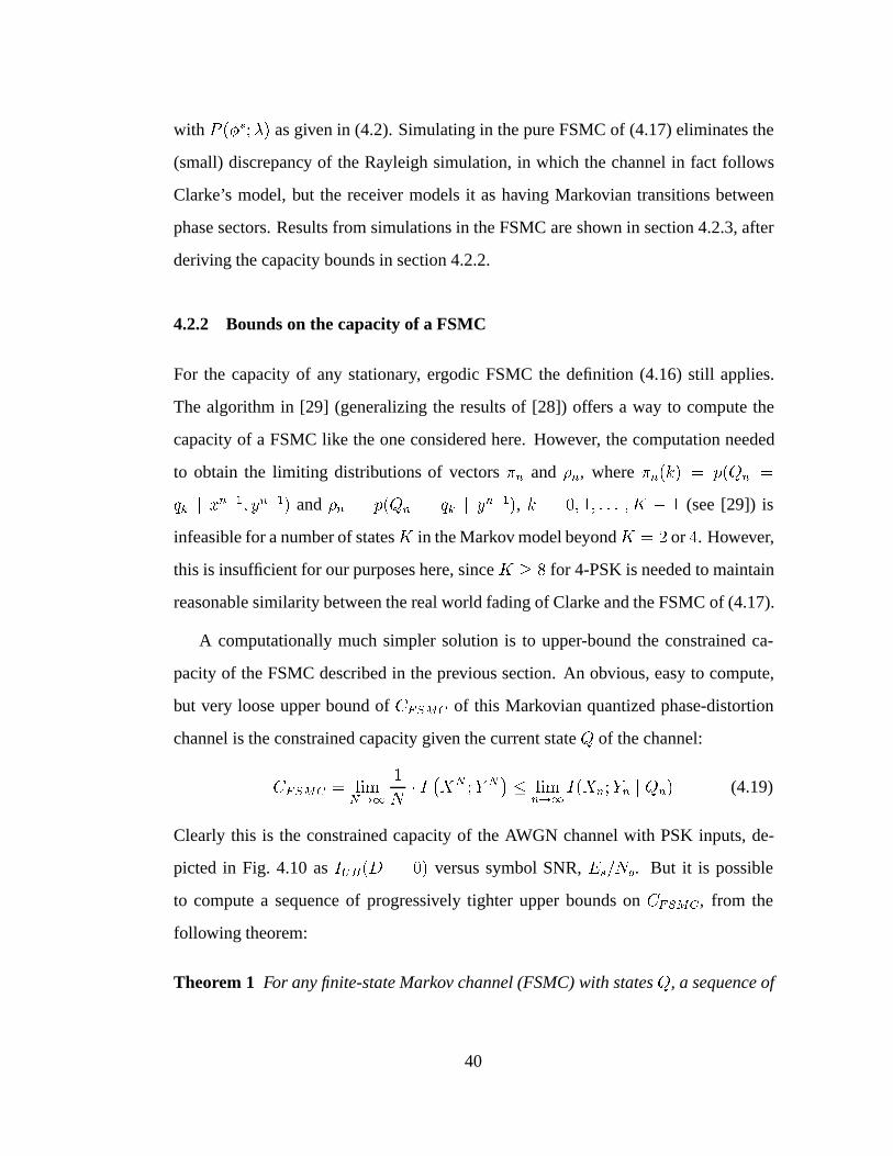
with P (��;�) as given in (4.2). Simulating in the pure FSMC of (4.17) eliminates the
(small) discrepancy of the Rayleigh simulation, in which the channel in fact follows
Clarke’s model, but the receiver models it as having Markovian transitions between
phase sectors. Results from simulations in the FSMC are shown in section 4.2.3, after
deriving the capacity bounds in section 4.2.2.
4.2.2 Bounds on the capacity of a FSMC
For the capacity of any stationary, ergodic FSMC the definition (4.16) still applies.
The algorithm in [29] (generalizing the results of [28]) offers a way to compute the
capacity of a FSMC like the one considered here. However, the computation needed
to obtain the limiting distributions of vectors �n and �n, where �n(k) = p(Qn =
qk j xn�1; yn�1) and �n = p(Qn = qk j yn�1), k = 0; 1; : : : ; K � 1 (see [29]) is
infeasible for a number of statesK in the Markov model beyondK = 2 or 4. However,
this is insufficient for our purposes here, since K � 8 for 4-PSK is needed to maintain
reasonable similarity between the real world fading of Clarke and the FSMC of (4.17).
A computationally much simpler solution is to upper-bound the constrained ca-
pacity of the FSMC described in the previous section. An obvious, easy to compute,
but very loose upper bound of CFSMC of this Markovian quantized phase-distortion
channel is the constrained capacity given the current state Q of the channel:
CFSMC = limN!1
1
N
� I �XN ;Y N� � lim
n!1I(Xn;Yn j Qn) (4.19)
Clearly this is the constrained capacity of the AWGN channel with PSK inputs, de-
picted in Fig. 4.10 as IUB(D = 0) versus symbol SNR, Es=No. But it is possible
to compute a sequence of progressively tighter upper bounds on CFSMC , from the
following theorem:
Theorem 1 For any finite-state Markov channel (FSMC) with states Q, a sequence of
40
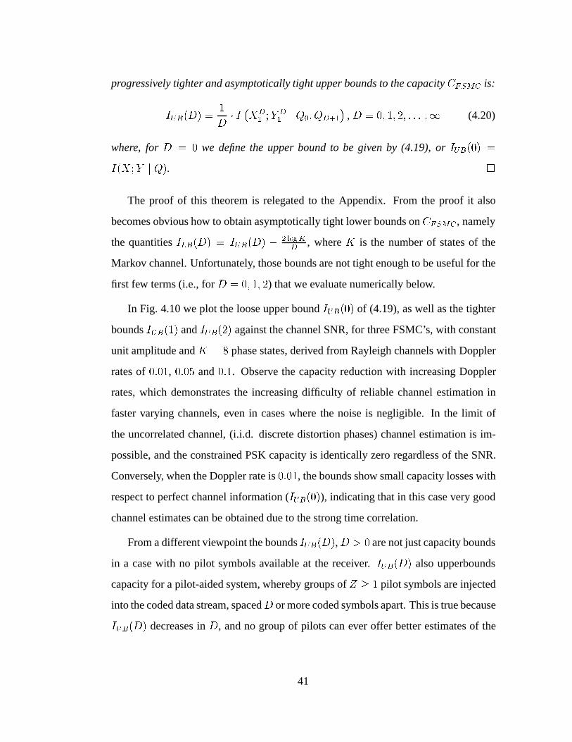
progressively tighter and asymptotically tight upper bounds to the capacity CFSMC is:
IUB(D) =1
D
� I �XD1 ;Y D
1 j Q0; QD+1
�, D = 0; 1; 2; : : : ;1 (4.20)
where, for D = 0 we define the upper bound to be given by (4.19), or IUB(0) =
I(X;Y j Q). �
The proof of this theorem is relegated to the Appendix. From the proof it also
becomes obvious how to obtain asymptotically tight lower bounds on CFSMC , namely
the quantities ILB(D) = IUB(D) � 2 logK
D, where K is the number of states of the
Markov channel. Unfortunately, those bounds are not tight enough to be useful for the
first few terms (i.e., for D = 0; 1; 2) that we evaluate numerically below.
In Fig. 4.10 we plot the loose upper bound IUB(0) of (4.19), as well as the tighter
bounds IUB(1) and IUB(2) against the channel SNR, for three FSMC’s, with constant
unit amplitude and K = 8 phase states, derived from Rayleigh channels with Doppler
rates of 0:01, 0:05 and 0:1. Observe the capacity reduction with increasing Doppler
rates, which demonstrates the increasing difficulty of reliable channel estimation in
faster varying channels, even in cases where the noise is negligible. In the limit of
the uncorrelated channel, (i.i.d. discrete distortion phases) channel estimation is im-
possible, and the constrained PSK capacity is identically zero regardless of the SNR.
Conversely, when the Doppler rate is 0:01, the bounds show small capacity losses with
respect to perfect channel information (IUB(0)), indicating that in this case very good
channel estimates can be obtained due to the strong time correlation.
From a different viewpoint the bounds IUB(D), D > 0 are not just capacity bounds
in a case with no pilot symbols available at the receiver. IUB(D) also upperbounds
capacity for a pilot-aided system, whereby groups of Z � 1 pilot symbols are injected
into the coded data stream, spacedD or more coded symbols apart. This is true because
IUB(D) decreases in D, and no group of pilots can ever offer better estimates of the
41
−4 −2 0 2 4 6 8 10 12 14 16 18 200
0.25
0.5
0.75
1
1.25
1.5
1.75
2
IUB
(D=0), AWGNIUB
(D=1) IUB
(D=2)
Symbol SNR Es=N
o, in dB
IU
B
(D)
from fDT = 0:1
from fDT = 0:05
from fDT = 0:01
Figure 4.10: Bounds on CFSMC for i.i.d. 4-PSK inputs, for Markov-phase channels
derived from three different Rayleigh channels with Doppler rates fDT , as described
in Chapter 3.
channel for t = 1; : : : ; D than noiseless knowledge of the channel states Q0; QD+1 at
the outer edges of each group of D information symbols.
4.2.3 Performance in the FSMC relative to capacity
This section presents the BER performance of the algorithms discussed in section 4.1,
simulated in the FSMC of (4.17). The only adaptation needed in the joint phase estima-
tion and turbo decoding algorithms for the supertrellis as well as the separate trellises
is shown in (4.18).
42
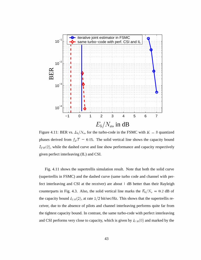
−1 0 1 2 3 4 5 6 7
10−4
10−3
10−2
10−1
iterative joint estimator in FSMC same turbo−code with perf. CSI and IL
Eb=N
o, in dB
BE
R
Figure 4.11: BER vs. Eb=No, for the turbo-code in the FSMC with K = 8 quantized
phases derived from fDT = 0:05. The solid vertical line shows the capacity bound
IUB(2), while the dashed curve and line show performance and capacity respectively
given perfect interleaving (IL) and CSI.
Fig. 4.11 shows the supertrellis simulation result. Note that both the solid curve
(supertrellis in FSMC) and the dashed curve (same turbo code and channel with per-
fect interleaving and CSI at the receiver) are about 1 dB better than their Rayleigh
counterparts in Fig. 4.3. Also, the solid vertical line marks the Eb=No = 0:2 dB of
the capacity bound IUB(2), at rate 1=2 bit/sec/Hz. This shows that the supertrellis re-
ceiver, due to the absence of pilots and channel interleaving performs quite far from
the tightest capacity bound. In contrast, the same turbo-code with perfect interleaving
and CSI performs very close to capacity, which is given by IUB(0) and marked by the
43
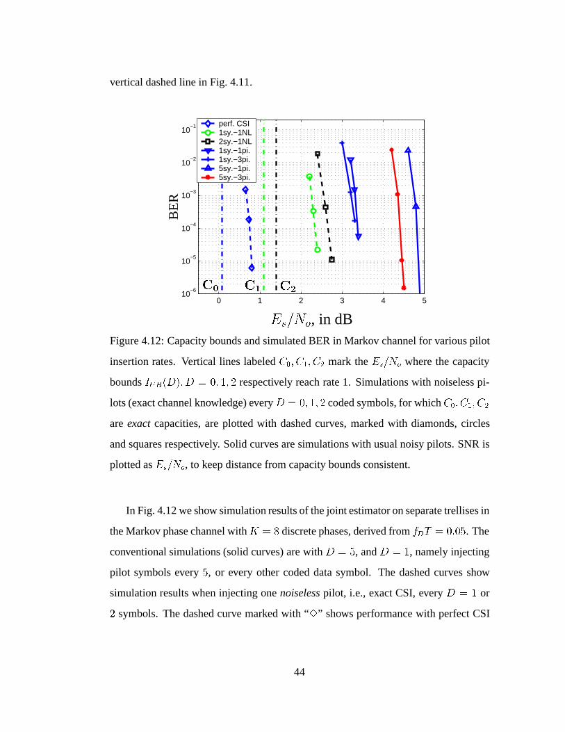
vertical dashed line in Fig. 4.11.
0 1 2 3 4 510
−6
10−5
10−4
10−3
10−2
10−1 perf. CSI
1sy.−1NL 2sy.−1NL 1sy.−1pi.1sy.−3pi.5sy.−1pi.5sy.−3pi.
BE
R
Es=N
o, in dB
C0 C1 C2
Figure 4.12: Capacity bounds and simulated BER in Markov channel for various pilot
insertion rates. Vertical lines labeled C0; C1; C2 mark the Es=No where the capacity
bounds IUB(D); D = 0; 1; 2 respectively reach rate 1. Simulations with noiseless pi-
lots (exact channel knowledge) every D = 0; 1; 2 coded symbols, for which C0; C1; C2
are exact capacities, are plotted with dashed curves, marked with diamonds, circles
and squares respectively. Solid curves are simulations with usual noisy pilots. SNR is
plotted as Es=No, to keep distance from capacity bounds consistent.
In Fig. 4.12 we show simulation results of the joint estimator on separate trellises in
the Markov phase channel with K = 8 discrete phases, derived from fDT = 0:05. The
conventional simulations (solid curves) are with D = 5, and D = 1, namely injecting
pilot symbols every 5, or every other coded data symbol. The dashed curves show
simulation results when injecting one noiseless pilot, i.e., exact CSI, every D = 1 or
2 symbols. The dashed curve marked with “3” shows performance with perfect CSI
44
everywhere. All three of these simulation scenarios are idealized, since no noiseless
pilots or perfect CSI can be available, but they are cases where the capacity bounds
IUB(D); D = 0; 1; 2 are no longer a bound, but the true capacity of these idealized
transmission situations. Observe that the distance of the “noiseless” pilot simulated
BER curves for D = 1 and 2 from the respective capacity bounds (dashed vertical
lines marked C1; C2) is the same, a consistent 1:3 dB. Also note, that performance
is plotted against symbol SNR Es=No, unlike previous curves, in order to show the
consistent SNR gap with respect to the capacity bounds.
The results of simulations in the Markov phase channel (those included in Fig. 4.12
and others) are summarized in Table 4.1 in the following fashion. The first column (D)
shows how many consecutive information symbols are transmitted into the channel
before Z = 1 or more (in the second column) consecutive pilot symbols are injected.
In cases marked “noisy” in the third column, the pilot symbols are conventional pilots,
offering noisy estimates of the channel at the edge-points of a D-symbol information
block. Cases marked “noiseless” (NL) refer to the unrealistic scenario of a noiseless
pilot, offering exact channel knowledge between groups of D symbols. For those cases
the bounds IUB(D) are no longer bounds, but the exact capacity for this idealized
transmission scheme. The fourth column of the table shows the Es=No in dB, at which
a BER of 10�4 is reached. The last two columns show the SNR gap between the
simulated performance and performance with perfect CSI everywhere, and the SNR
gap from the tightest appropriate capacity bound computed in section 4.2.2. Observe
that the gap from the capacity bounds is smaller than that from perfect CSI, which
shows that in this noisy, fast-varying channel the performance with perfect CSI is not
achievable. For the first 3 rows, the correct capacity bound is C1 = 1:1 dB, i.e., the
Es=No where IUB(D = 1) reaches rate 1. For all other rows, the tightest bound is
C2 = 1:4 dB, i.e., the SNR at which IUB(D = 2) reaches rate 1.
45
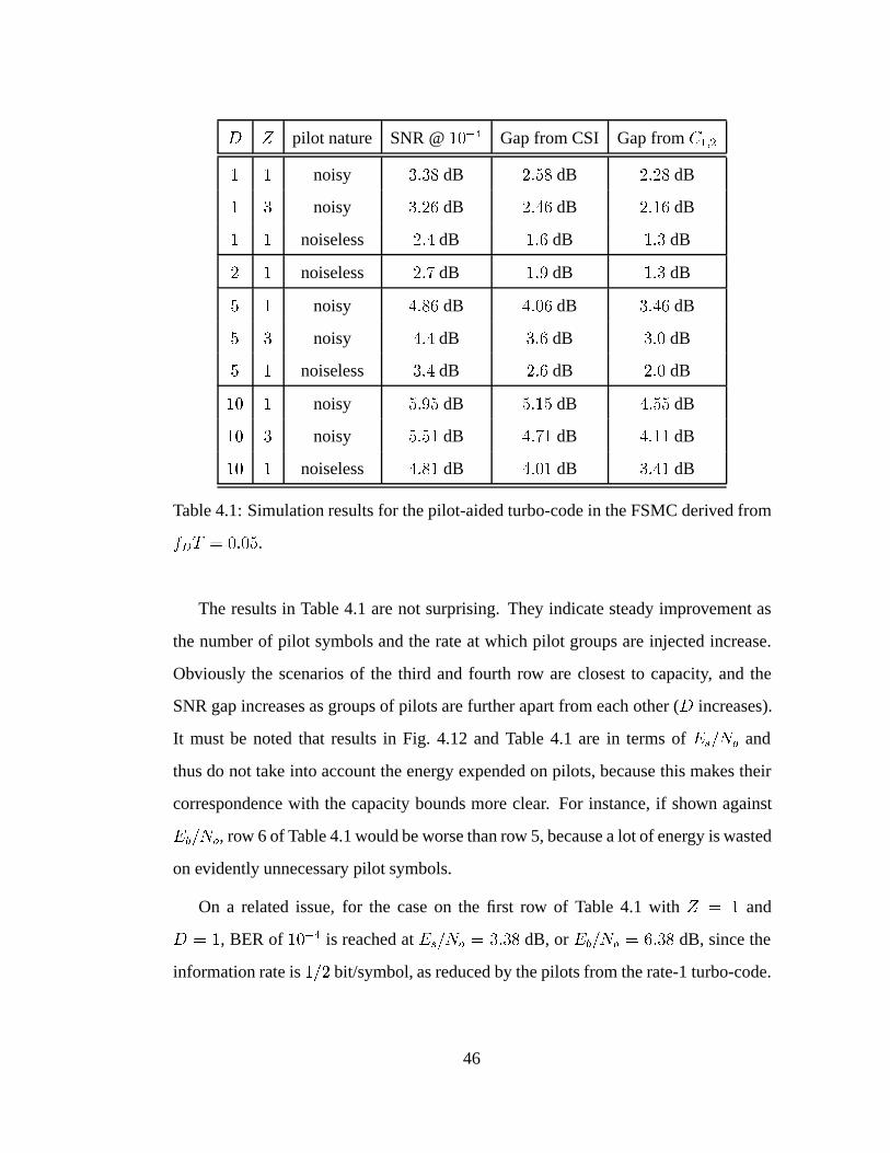
D Z pilot nature SNR @ 10�4 Gap from CSI Gap from C1;2
1 1 noisy 3:38 dB 2:58 dB 2:28 dB
1 3 noisy 3:26 dB 2:46 dB 2:16 dB
1 1 noiseless 2:4 dB 1:6 dB 1:3 dB
2 1 noiseless 2:7 dB 1:9 dB 1:3 dB
5 1 noisy 4:86 dB 4:06 dB 3:46 dB
5 3 noisy 4:4 dB 3:6 dB 3:0 dB
5 1 noiseless 3:4 dB 2:6 dB 2:0 dB
10 1 noisy 5:95 dB 5:15 dB 4:55 dB
10 3 noisy 5:51 dB 4:71 dB 4:11 dB
10 1 noiseless 4:81 dB 4:01 dB 3:41 dB
Table 4.1: Simulation results for the pilot-aided turbo-code in the FSMC derived from
fDT = 0:05.
The results in Table 4.1 are not surprising. They indicate steady improvement as
the number of pilot symbols and the rate at which pilot groups are injected increase.
Obviously the scenarios of the third and fourth row are closest to capacity, and the
SNR gap increases as groups of pilots are further apart from each other (D increases).
It must be noted that results in Fig. 4.12 and Table 4.1 are in terms of Es=No and
thus do not take into account the energy expended on pilots, because this makes their
correspondence with the capacity bounds more clear. For instance, if shown against
Eb=No, row 6 of Table 4.1 would be worse than row 5, because a lot of energy is wasted
on evidently unnecessary pilot symbols.
On a related issue, for the case on the first row of Table 4.1 with Z = 1 and
D = 1, BER of 10�4 is reached at Es=No = 3:38 dB, or Eb=No = 6:38 dB, since the
information rate is 1=2 bit/symbol, as reduced by the pilots from the rate-1 turbo-code.
46

The same BER at the same information rate is achieved at Eb=No � 7:0 dB with the
supertrellis receiver, see Fig. 4.11, because the turbo-code there is of rate-1/2. This
performance improvement of at least 0:6 dB highlights the positive effect of channel
interleaving in providing diversity for the separate trellises approach, despite the larger
complexity of the supertrellis.
47
CHAPTER 5
Diversity Reception in Flat Fading
For a general multipath fading channel, reception errors usually occur when the time-
varying signal attenuation introduced by the channel is large, or when the channel is
in a deep fade. A good strategy to overcome this problem is to provide the receiver
with several replicas of the information signal, transmitted over independently fading
channels, and hence reduce the probability that all signal components will fade simul-
taneously [30]. The presence of conditionally independent replicas of the information-
bearing signal at the receiver is called diversity. There are three common types of
diversity: frequency, time and space. Frequency diversity is only possible if the trans-
mission bandwidth exceeds the channel coherence bandwidth —i.e., it is not available
in flat fading. An equalizer, a RAKE receiver [31, 32], or coded multicarrier transmis-
sion [33] can exploit frequency diversity. Time-diversity is often accomplished with
coding and interleaving; trellis codes do the same in a bandwidth-efficient fashion.
Spatial diversity is achieved by using multiple receiver antennas. This form of diver-
sity avoids the bandwidth expansion implicit in frequency and (often) time diversity,
but requires additional complexity in the RF and baseband portions of the receiver.
This chapter extends the algorithm for joint phase estimation and turbo-decoding
on separate trellises, derived in Chapter 4, to the case where several (L � 1) branches
of spatial diversity are available at the receiver, thus simultaneously exploiting antenna
diversity and time-diversity with the turbo-code. In this scenario, the utilization of
the L soft channel estimates provided by the quantized phase estimators to the turbo-
48
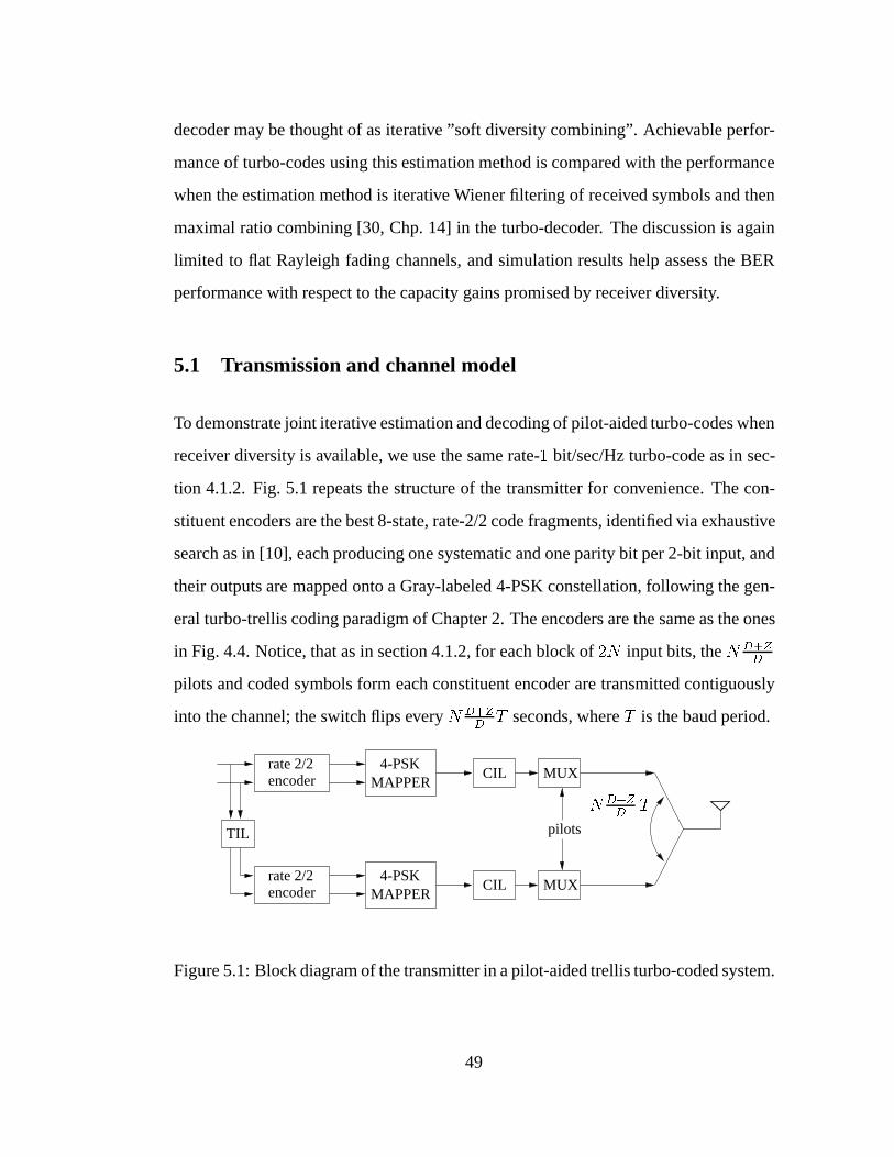
decoder may be thought of as iterative ”soft diversity combining”. Achievable perfor-
mance of turbo-codes using this estimation method is compared with the performance
when the estimation method is iterative Wiener filtering of received symbols and then
maximal ratio combining [30, Chp. 14] in the turbo-decoder. The discussion is again
limited to flat Rayleigh fading channels, and simulation results help assess the BER
performance with respect to the capacity gains promised by receiver diversity.
5.1 Transmission and channel model
To demonstrate joint iterative estimation and decoding of pilot-aided turbo-codes when
receiver diversity is available, we use the same rate-1 bit/sec/Hz turbo-code as in sec-
tion 4.1.2. Fig. 5.1 repeats the structure of the transmitter for convenience. The con-
stituent encoders are the best 8-state, rate-2/2 code fragments, identified via exhaustive
search as in [10], each producing one systematic and one parity bit per 2-bit input, and
their outputs are mapped onto a Gray-labeled 4-PSK constellation, following the gen-
eral turbo-trellis coding paradigm of Chapter 2. The encoders are the same as the ones
in Fig. 4.4. Notice, that as in section 4.1.2, for each block of 2N input bits, the N D+ZD
pilots and coded symbols form each constituent encoder are transmitted contiguously
into the channel; the switch flips every N D+ZD
T seconds, where T is the baud period.
rate 2/2encoder
4-PSKMAPPER
rate 2/2encoder
4-PSKMAPPER
TIL
CIL
CIL
MUX
MUX
pilots
ND+ZD
T
Figure 5.1: Block diagram of the transmitter in a pilot-aided trellis turbo-coded system.
49
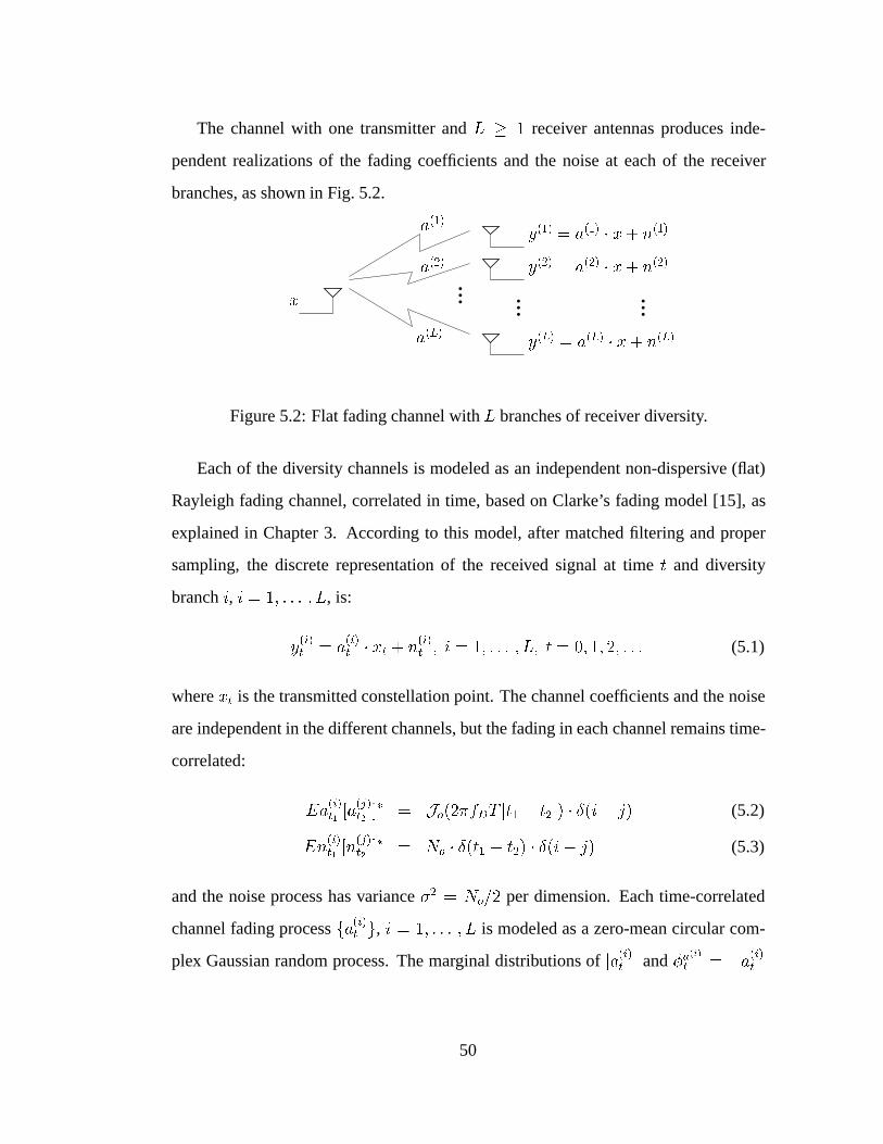
The channel with one transmitter and L � 1 receiver antennas produces inde-
pendent realizations of the fading coefficients and the noise at each of the receiver
branches, as shown in Fig. 5.2.
... ... ...x
a(L)
a(2)
a(1)
y(1) = a
(1) � x + n(1)
y(2) = a
(2) � x + n(2)
y(L) = a
(L) � x + n(L)
Figure 5.2: Flat fading channel with L branches of receiver diversity.
Each of the diversity channels is modeled as an independent non-dispersive (flat)
Rayleigh fading channel, correlated in time, based on Clarke’s fading model [15], as
explained in Chapter 3. According to this model, after matched filtering and proper
sampling, the discrete representation of the received signal at time t and diversity
branch i, i = 1; : : : ; L, is:
y
(i)t = a
(i)t � xt + n
(i)t ; i = 1; : : : ; L; t = 0; 1; 2; : : : (5.1)
where xt is the transmitted constellation point. The channel coefficients and the noise
are independent in the different channels, but the fading in each channel remains time-
correlated:
Ea
(i)t1[a
(j)t2]� = Jo(2�fDT jt1 � t2j) � �(i� j) (5.2)
En
(i)t1[n
(j)t2]� = No � �(t1 � t2) � �(i� j) (5.3)
and the noise process has variance �2 = No=2 per dimension. Each time-correlated
channel fading process fa(i)t g, i = 1; : : : ; L is modeled as a zero-mean circular com-
plex Gaussian random process. The marginal distributions of ja(i)t j and �a(i)
t = \a(i)t
50
for each i are Rayleigh and uniform respectively [17], hence the term “Rayleigh fad-
ing”. The correlation properties of each fading processes a(i)t , i = 1; : : : ; L —see
(5.2)— depend on the common Doppler rate fDT for all receiver branches, since they
are probably mounted on the same physical device and move simultaneously.
5.2 General iterative receiver
Given the turbo-coded, pilot-aided transmission model of Fig. 5.1, the block diagram
of a generic receiver with iterative channel estimation and diversity of order L is de-
picted in Fig. 5.3.
The blocks “D1” and “D2” are the constituent decoders (SISOs) for the turbo-code,
and they implement the Forward-Backward algorithm. They exchange extrinsic infor-
mation (P (u; I); P (u;O)) about the 2-bit input symbols u through the uniform random
interleaver/deinterleaver pair TIL/TDIL. At the same time they produce extrinsic in-
formation P (x;O) about the coded symbols x, in order to assist the channel estimation
procedure on all diversity branches. Estimation is performed by the array of identical
modules E1i;E2i, i = 1; : : : ; L. For the functionality of these estimation blocks, this
chapter considers two options.
In the first approach, henceforth dubbed the “quantized approach”, (dashed feed-
back path in Fig. 5.3) no operation other than channel deinterleaving is performed on
the probability vectors P (x;O) before they are fed back into the estimator modules.
They, in turn, produce probability vectors about the quantized channel phase, in exactly
the same fashion as the Q-SISO blocks described in Chapter 4. In the second itera-
tive estimation algorithm, the “filtering approach”, (solid feedback line in Fig. 5.3) the
vector of soft information P (x;O)—each entry of this vector is the extrinsic proba-
bility of a possible constellation point x—passes through the nonlinearity “NonLin”,
51
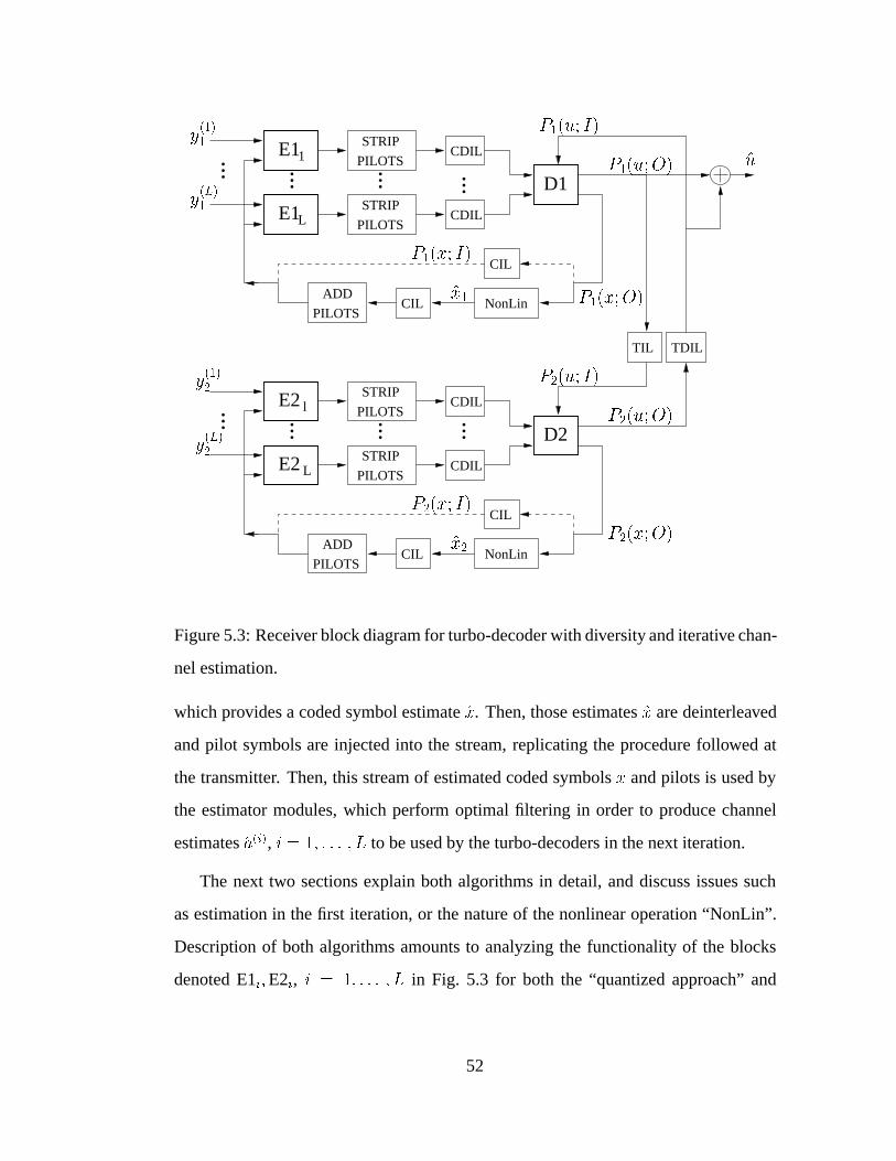
STRIP
PILOTSCDIL
STRIP
PILOTSCDIL
ADD
PILOTSCIL NonLin
STRIP
PILOTSCDIL
STRIP
PILOTSCDIL
ADD
PILOTSCIL NonLin
CIL
CIL
E1
D1
E1
D2
E2
E2
TDIL
L
L
1
l
... ... ... ...
... ... ...
TIL
...
P1(u; I)
P2(u; I)
P2(x;O)
P1(u;O)
P2(u;O)
x1
x2
u
P1(x;O)
y(1)1
y(L)1
y(1)2
y(L)2
P1(x; I)
P2(x; I)
Figure 5.3: Receiver block diagram for turbo-decoder with diversity and iterative chan-
nel estimation.
which provides a coded symbol estimate x. Then, those estimates x are deinterleaved
and pilot symbols are injected into the stream, replicating the procedure followed at
the transmitter. Then, this stream of estimated coded symbols x and pilots is used by
the estimator modules, which perform optimal filtering in order to produce channel
estimates a(i), i = 1; : : : ; L to be used by the turbo-decoders in the next iteration.
The next two sections explain both algorithms in detail, and discuss issues such
as estimation in the first iteration, or the nature of the nonlinear operation “NonLin”.
Description of both algorithms amounts to analyzing the functionality of the blocks
denoted E1i;E2i, i = 1; : : : ; L in Fig. 5.3 for both the “quantized approach” and
52
the “filtering approach”, as well as the corresponding metric used by the constituent
decoders “D1” and “D2” in conjunction with each channel estimation method.
5.2.1 Quantized phase approach
For PSK transmission the acquisition of phase coherence is a more critical problem
than fading amplitude estimation, as discussed in Chapter 3. Thus, the quantized
phase algorithm invests most of the computational effort into obtaining an accurate
probability distribution Pi(q;O) on the quantized phases q = Q
��a(i)�
of each diver-
sity channel i = 1; : : : ; L via the Forward-Backward algorithm. Thus, each estimation
module E1i;E2i of Fig. 5.3 becomes a Q-SISO, described in Chapter 4. For an esti-
mate of the fading amplitude��a(i)�� each Q-SISO uses a simple, symbol-by-symbol
optimum affine estimator from the received amplitude, namely:
[ja(i)j = A � jy(i)j+B; i = 1; : : : ; L (5.4)
where A, B are real coefficients depending on the SNR (hence the same for all i), and
they are computed to ensure unbiasedness and MMSE of the amplitude estimates.
For the phase estimation, each Q-SISO considers the quantized version of the chan-
nel phase �a(i)
into K phase intervals as in section 4.1.2. All the Q-SISOs (there are
2L of them in the receiver) create the same Markov model, which approximates the
values and the statistical properties of each �a(i)
. The transition probabilities between
phase sectors depend on the common Doppler rate fDT , and can be computed as in
(3.5)-(3.6). Fig. 5.4 provides an example of the Markovian transition probabilities for
the quantized phase, as derived for two Doppler rates.
Given the quantized version q of the channel phase�q = 2�j
K; j = 0; 1; : : : ; K � 1
�,
the ith Q-SISO considers the real-valued phase �a(i)
to be uniformly distributed within
the interval�q � �
K; q + �
K
�. Then, recall from Fig. 4.1 that on each diversity branch
53
0:75045
0:11326
0:11326
0:02714
0:02714
0:94478
Figure 5.4: Transition probabilities for fDT = 0:05 (left) and fDT = 0:01 (right), for
K = 8 quantized phases.
the received angle �(i) = \y(i)t at time t is the sum of the common transmitted angle
\xt, the fading angle �a(i)
t and the noise induced angle ��(i)
t , distributed as in (4.2).
With that in mind, as in section 4.1.2, each Q-SISO runs the Forward-Backward
algorithm on the trellis of the quantized Markovian channel phases, and produces
probabilities Pi(q;O) for those quantized phases q, on each diversity channel i, i =
1; : : : ; L. To do that, following the derivation in (4.14) and using (4.5), it is straight-
forward for the ith Q-SISO to compute the branch metric (i)t (q0; q) as follows:
(i)t (q0; q)
def= Pr
�y
(i)t =
���y(i)t ��� ej�(i); q(i)t = q j q(i)t�1 = q0�
(5.5)
= P (q0 ! q)�Xx
P (x; I) � K2�
Z �(i)�\x�q+ �K
�(i)�\x�q� �K
P
���;�
(i)t
�d�
�(5.6)
where P (��;�) was given in (4.2) and �
(i)t is approximated, using the estimate[ja(i)j
from (5.4), by:
c�
(i)t =
A
���y(i)t ���+B
�
p2
(5.7)
Thus, using the precomputed Markovian transition probabilities P (q0 ! q), as
well as the extrinsics P (x; I) fed back by the constituent turbo-decoder “D1” or “D2”,
54
each Q-SISO is able to provide the desired extrinsic information Pi(q;O) about the
quantized channel phase in each diversity branch. Those L distinct vectors of extrinsic
probabilities Pi(q;O), i = 1; : : : ; L are subsequently deinterleaved and passed to the
turbo-decoder (“D1” or “D2”), as shown in Fig. 5.3.
At the first iteration, when no prior P (x; I) is available, all inputs P (x; I) to the
Q-SISOs are set to zero (in the log domain), denoting equal probabilities, with the
exception of points t in time which belong to a pilot slot. Since the pilot symbol is
known a priori, each Q-SISO uses the most skewed pmf there, setting the probability
of the pilot symbol to a very large number (certainty) and the others to zero. This
special handling of the pilots also carries over to subsequent iterations of the estimation
procedure. Thus, for pilots, the summation of (5.6) is trivial (only one possible x
has non-zero probability). At times t corresponding to coded data and not pilots the
summation of (5.6) is necessary to compute the correct branch metric (i)t (q0; q) and
run the Forward-Backward algorithm in each Q-SISO.
At every time t, each constituent decoder (“D1” or “D2” in Fig. 5.3) receives
from the L Q-SISOs after deinterleaving the L vectors Pi(q; I), i = 1; : : : ; L, each
of length K—the number of quantized phase states. These K-entry vectors Pi(q; I),
i = 1; : : : ; L, contain the soft information about the quantized channel phase q(i) on
each of the diversity branches, so denote their entries:
P
�q(i); I
�; q
(i) = 0; : : : ; K � 1; i = 1; : : : ; L: (5.8)
For ease of notation, boldface letters denote the L-length vectors of the received (dein-
terleaved) samples and the quantized phases: yt = [y(1)t : : : y
(L)t ] and qt = [q
(1)t : : : q
(L)t ].
Clearly, the “vector phase-state” qt of the L-branch diversity channel can take one of
anyKL possible values. Given the independence between diversity channels, the prob-
55

ability of the channel vector-state is:
P (qt = q) =
LYi=1
P (q(i); I): (5.9)
Thus, the constituent decoder can run the Forward-Backward algorithm on the
code trellis, and compute the branch metric t(c0; c), based on the vector observations
yt. Since the channel estimates obtained from the Q-SISOs are not hard estimates
a(i) of the fading coefficients, but soft estimates, i.e. probabilities that the channel
phase is in one of K sectors, the decoder performs soft-diversity combining. With this
quantized approach, and denoting the code states as c0 and c, each decoder (“D1” or
“D2”) computes the Forward-Backward branch metric t(c0; c) as follows:
t(c0; c) = Pr (yt; Ct = cj Ct�1 = c
0) (5.10)
= P (ut such that c0 ! c) � P (yt j x(c0 ! c)) (5.11)
= P (u; I) �Xq
P (yt;qt = q j x(c0 ! c)) (5.12)
= P (u; I) �Xq
P (qt = q) � P (yt j x(c0 ! c);q) (5.13)
= P (u; I) �X
q(1);::: ;q(L)
LYi=1
P (q(i); I) � P�y
(i)t j x(c0 ! c); q(i)
�(5.14)
= P (u; I) �X
q(1);::: ;q(L)
LYi=1
P (q(i); I) � K2�
Z �(i)�\x�q+ �K
�(i)�\x�q� �K
P (��;�(i)t )d��
Of the terms in the above formula, P (u; I) is the extrinsic information about the input
symbol u and is provided by the other constituent decoder, while P (q(i); I) is provided
by the ith Q-SISO. The summation involves KL distinct terms, each of which is the
product of two terms, as shown in (5.14). Hence, the constituent decoder “D1” (or
“D2”) essentially performs soft combining of the quantized soft channel estimates
coming from the estimators E1i, i = 1; : : : ; L (or E2i, i = 1; : : : ; L), which are
all identical Q-SISO modules.
56
Due to the soft combining of channel estimates, the complexity of the quantized
approach is quite high. For L = 2 diversity branches at the receiver, every full iteration
of the joint estimator and turbo-decoder involves 2L = 4 Forward-Backward runs on
the K-state Q-SISOs (8 states here) with branch metrics computed as in (5.5)-(5.6),
as well as two Forward-Backward runs on the 8-state constituent decoders “D1” and
“D2” with branch metrics computed as in (5.10)-(5.14). Note that, because of the op-
eration in the log-domain, multiplications in the above formulas become summations
and summations become the max� operation (2.13). However, complexity is still an
issue, so we limit the number of quantized phases to K = 8 (twice the cardinality of
the 4-PSK constellation). The performance of this receiver is presented in section 5.3.
5.2.2 Optimum filtering approach
This section describes an alternative approach for iterative joint channel estimation
and decoding, based on optimum filtering of received symbols (only pilots at the first
iteration, coded symbols and pilots alike in subsequent iterations). Iterative filtering
solutions have been proposed in [21] and in [20] for low-rate turbo-codes with BPSK
constellations. The treatment here is general, and in fact can also cover non-PSK
constellations, unlike the quantized phase approach in section 5.2.1. Nevertheless,
we limit our simulations in section 5.3 to the familiar 8-state, 4-PSK turbo-code of
Fig. 4.4.
With the filtering approach, the solid feedback lines in Fig. 5.3 are active (the
dashed lines refer to the quantized phase approach). The purpose of the channel esti-
mation modules E1i, E2i, i = 1; : : : ; L, is to obtain estimates for the complex channel
gains a(i)1 , a(i)2 , i = 1; : : : ; L, and provide those estimates (after deinterleaving) to the
appropriate constituent decoder “D1” or “D2”. For this purpose, each estimator E1i
(or E2i) performs optimum (Wiener) filtering of received symbols at every iteration.
57
Intuitively, as decoder iterations proceed and more reliable knowledge about the coded
symbols x is obtained, the estimators are able to provide better estimates of the channel
gains a(i), in turn contributing to a better performance by the constituent decoders.
In the first iteration, when no knowledge about the transmitted symbols x, other
than the pilots, is available, the estimators E1i, E2i, i = 1; : : : ; L are pilot filters. These
filters are identical for all 2L diversity branches, and are derived as in Appendix A,
given the filter length, the Doppler rate fDT , the number D of coded symbols between
pilot slots, the number Z of pilot symbols per slot, and the SNR. Specifically, the pilot-
only filter (POF) W ok (where k = 0; 1; : : : ; D � 1 specifies the time index within the
coded data slot between two adjacent pilot slots that the filter W ok is intended for) is an
FIR filter, represented as a horizontal vector in (A.2):
Wok = Rak ;~y �R�1
~y ; k = 0; 1; : : : ; D � 1; (5.15)
where the entries of vectorRak ;~y and matrixR~y are computed in Appendix A. ThoseD
distinct POFs are computed once, at the beginning of the simulation, and subsequently
used for the first iteration of every turbo-coded block, by all 2L estimators. They filter
received samples corresponding to pilots only (denote them ~y(i) after derotation of y(i)
with the known pilot symbol x) and produce channel estimates a(i)1 , i = 1; : : : ; L (and
a
(i)2 , i = 1; : : : ; L) to be used by the constituent decoders “D1” (and “D2”respectively).
Now consider how the constituent decoder “D1” (the same holds for “D2”, so we
suppress the subscripts) uses the channel estimates a(i), i = 1; : : : ; L, after deinter-
leaving, to compute the metric t(c0; c). In essence the decoder performs maximal
ratio combining of the L received samples y(i)t , i = 1; : : : ; L, collected in the vector
58
yt as follows:
t(c0; c) = Pr (yt; Ct = cj Ct�1 = c
0) (5.16)
= P (ut such that c0 ! c) � P (yt j at; x(c0 ! c)) (5.17)
= P (u; I) � (�G1) � kyt � at x(c0 ! c)k2 (5.18)
= P (u; I) �G2 ��2Rfy�t at x(c0 ! c)g � katk2jx(c0 ! c)j2�; (5.19)
where at is the L-length vector comprising the estimates a(i), i = 1; : : : ; L, and Rf�gdenotes the real part, and G1, G2 are irrelevant nonnegative constants. Note that in the
case of PSK transmission, where all symbols x are of equal energy, the metric (5.19)
can take the simpler form:
t(c0; c) = P (u; I) � R fy�t at x(c0 ! c)g : (5.20)
It is obvious that, although the inner product y�t at in (5.20) above involves L com-
plex multiplications, the metric derived above for the decoder in the iterative filtering
approach is still much simpler than the one in (5.14) for the “quantized approach”.
However, some additional complexity ensues in the filtering approach after the
first iteration. The reason is that the estimation modules E1i, E2i, i = 1; : : : ; L need
estimates of the coded symbols (call those estimates x) and cannot exploit the vectors
P (x;O) of extrinsic information about x, which is what the decoders “D1” and “D2”
provide. This is why the nonlinearity “NonLin” is included in the (solid) feedback
paths of Fig. 5.3. The purpose of this nonlinearity is to use the vector of probabilities
P (x;O) for every t and provide a hard estimate x for the coded symbol x, such that
the filters E1i, E2i can use x to improve their channel estimates in the next iteration.
A simple way to obtain x is to simply choose as x the constellation point xm with
the maximum P (x;O), or:
x = xm () P (xm;O) � P (xl; 0); l = 0; 1; : : : ;M � 1; l 6= m; (5.21)
59
where M is the constellation size. We refer to this type of nonlinearity as hard tentative
decoding. A better way to obtain x is to use the soft information in P (x;O) in a more
sophisticated fashion. Recall that the entries of the vector P (x;O) at each time are the
log-probabilities of every constellation point x. Hence, it makes sense to set:
x =
M�1Xl=0
Pr(xl) � xl =M�1Xl=0
eP (xl;O) � xl: (5.22)
In the simulations results presented in the next section we use the nonlinearity of
(5.22), but the performance degradation if the simpler (5.21) is used is very small.
After the estimates for the coded symbols x have been produced for the whole
block, the receiver replicates the operations of the transmitter, by interleaving them
and adding pilot symbols (refer to Fig. 5.3, solid feedback path). So, at the input of
the estimation blocks E1i, E2i, i = 1; : : : ; L, we now have an approximated replica of
the transmitted sequence. In all iterations but the first, the estimators use this sequence
to derotate the received samples y(i)1 , y(i)2 , i = 1; : : : ; L, so that Wiener filtering of
the derotated ~y(i)1 , ~y(i)2 can follow, to produce new channel estimates a(i)1 , a(i)2 . We call
each of those Wiener filters—they are the same on all 2L diversity branches—an “all-
symbol filter” (ASF), to distinguish it from the pilot-only filter (POF) Wo of (5.15),
which is used only at the first iteration.
The ASF is easier to compute than the POF, because it only filters derotated sam-
ples that passed through the channel at adjacent times, unlike the POF, which only
filters pilots. Moreover, there is only a single ASF for every time t, while a differ-
ent POF Wok was needed for every position k = 0; 1; : : : ; D � 1 between pilot slots.
Assume the ASF is an FIR filter with 2L1 + 1 coefficients, stored in the vector Zo.
Then, from linear estimation theory (see [34]) and given the SNR and Doppler rate,
the optimum ASF is given by:
Zo = Eak~y
� � [E~y~y�]�1
= Rak ;~y �R�1~y ; (5.23)
60
where, analogous to Appendix A, ~y is a vector containing 2L1 + 1 derotated consecu-
tive received samples:
~y = [~yk�L1~yk�L1+1 : : : ~yk+L1
]T= a + ~n (5.24)
Hence, the entries of the horizontal vector Rak;~y are:
Rak;~y(n) = Jo (2�fDT � jL1 � nj) ; n = 0; 1; : : : ; 2L1; (5.25)
where Jo(�) is the zero-order modified Bessel function of the first kind and the matrix
R~y is:
R~y = Ra + 2�2I2L1+1; (5.26)
where the matrix Ra = Eaa� is symmetric and Toeplitz, with entries:
Ra(n;m) = Jo (2�fDT � jn�mj) ; n;m = 0; 1; : : : ; 2L1: (5.27)
The ASF Zo operates for every time t and at every diversity branch to yield updated
channel estimates:
a
(i)t = Z
o �h~y(i)
t�L1~y(i)
t�L1+1 : : : ~y(i)
t+L1
iT; i = 1; : : : ; L; t = 0; 1; 2; : : : ; N � 1;
which are subsequently deinterleaved and provided to decoder “D1” or “D2” for the
next algorithm iteration. The above filtering equation ignores the “edge-effects” at
the beginning and end of turbo-coded blocks of N symbols, where there are not
enough samples on either side of the symbol of interest to support two-sided filter-
ing (i.e. smoothing). The same is true for pilot-only filtering and the POF in (5.15),
which is also a two-sided filter (smoother). However, this problem can easily be solved
either via inclusion of a few additional pilots at the edges of each block, or by design-
ing special optimum filters to take into account those edge-effects. This is a minor
problem for the filtering approach (also noticed in [21]), and it does not exist at all in
the “quantized approach” because of the Markov approximation of the channel phase.
61
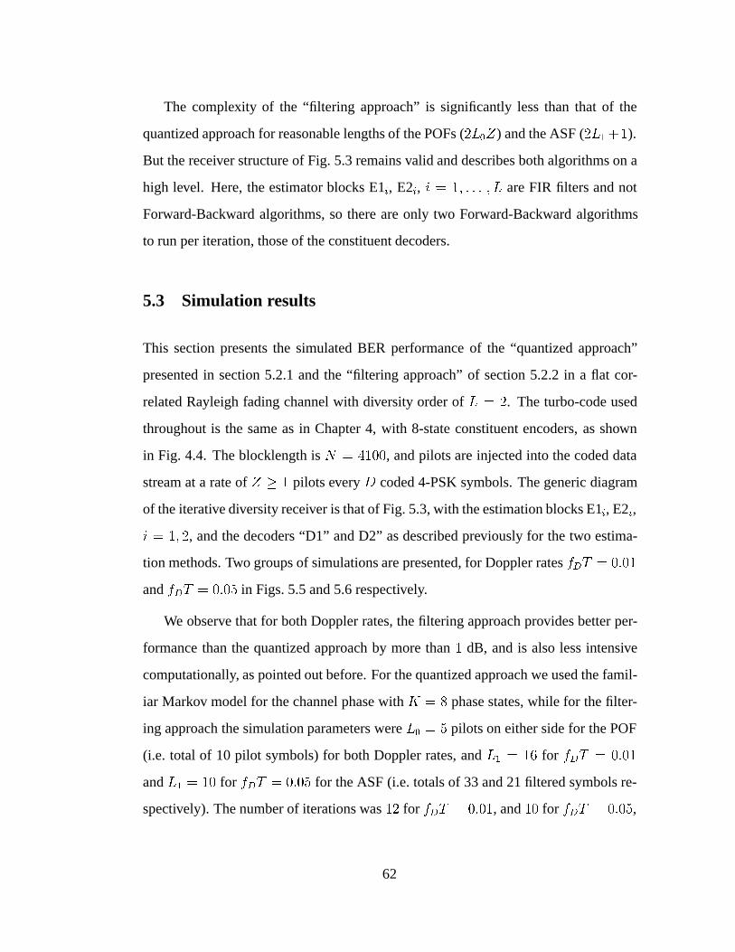
The complexity of the “filtering approach” is significantly less than that of the
quantized approach for reasonable lengths of the POFs (2L0Z) and the ASF (2L1+1).
But the receiver structure of Fig. 5.3 remains valid and describes both algorithms on a
high level. Here, the estimator blocks E1i, E2i, i = 1; : : : ; L are FIR filters and not
Forward-Backward algorithms, so there are only two Forward-Backward algorithms
to run per iteration, those of the constituent decoders.
5.3 Simulation results
This section presents the simulated BER performance of the “quantized approach”
presented in section 5.2.1 and the “filtering approach” of section 5.2.2 in a flat cor-
related Rayleigh fading channel with diversity order of L = 2. The turbo-code used
throughout is the same as in Chapter 4, with 8-state constituent encoders, as shown
in Fig. 4.4. The blocklength is N = 4100, and pilots are injected into the coded data
stream at a rate of Z � 1 pilots every D coded 4-PSK symbols. The generic diagram
of the iterative diversity receiver is that of Fig. 5.3, with the estimation blocks E1i, E2i,
i = 1; 2, and the decoders “D1” and D2” as described previously for the two estima-
tion methods. Two groups of simulations are presented, for Doppler rates fDT = 0:01
and fDT = 0:05 in Figs. 5.5 and 5.6 respectively.
We observe that for both Doppler rates, the filtering approach provides better per-
formance than the quantized approach by more than 1 dB, and is also less intensive
computationally, as pointed out before. For the quantized approach we used the famil-
iar Markov model for the channel phase with K = 8 phase states, while for the filter-
ing approach the simulation parameters were L0 = 5 pilots on either side for the POF
(i.e. total of 10 pilot symbols) for both Doppler rates, and L1 = 16 for fDT = 0:01
and L1 = 10 for fDT = 0:05 for the ASF (i.e. totals of 33 and 21 filtered symbols re-
spectively). The number of iterations was 12 for fDT = 0:01, and 10 for fDT = 0:05,
62
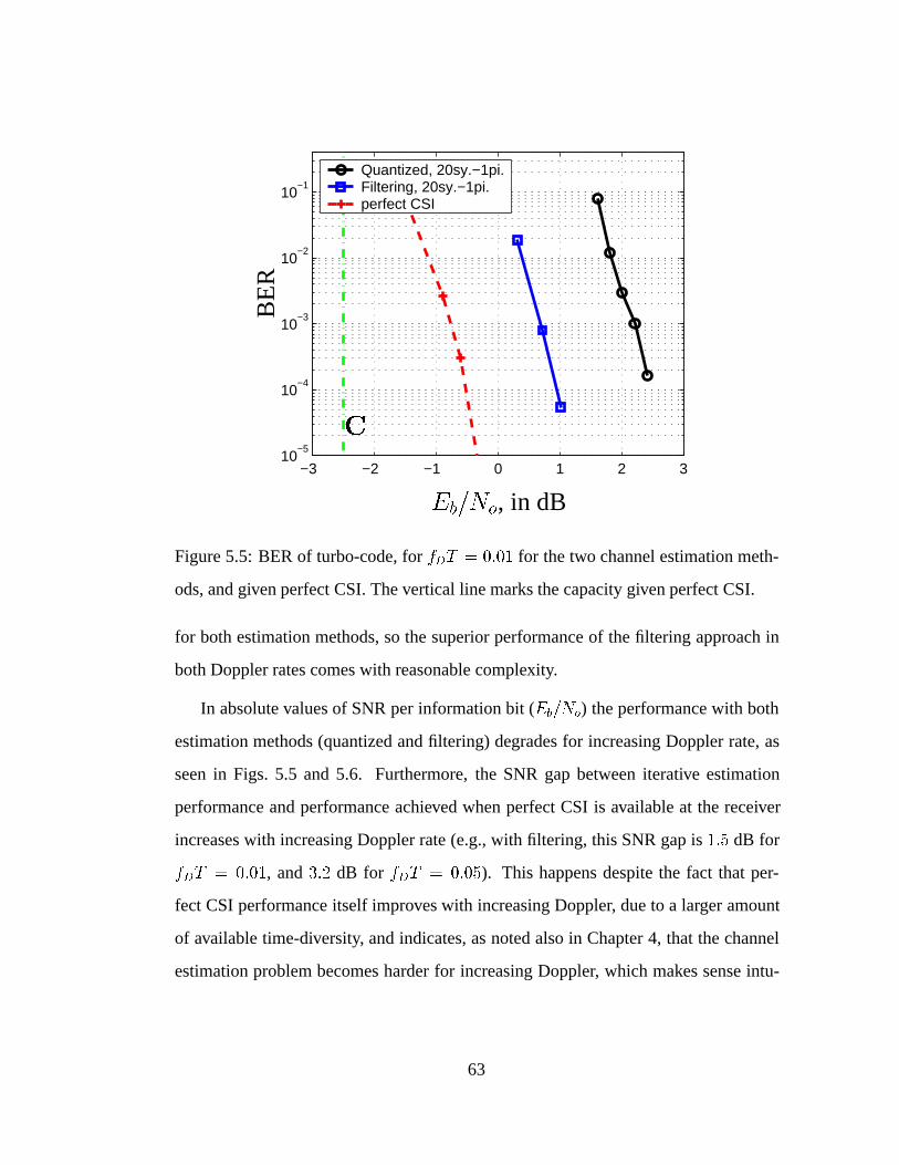
−3 −2 −1 0 1 2 310
−5
10−4
10−3
10−2
10−1
Quantized, 20sy.−1pi.Filtering, 20sy.−1pi.perfect CSI
BE
R
C
Eb=N
o, in dB
Figure 5.5: BER of turbo-code, for fDT = 0:01 for the two channel estimation meth-
ods, and given perfect CSI. The vertical line marks the capacity given perfect CSI.
for both estimation methods, so the superior performance of the filtering approach in
both Doppler rates comes with reasonable complexity.
In absolute values of SNR per information bit (Eb=No) the performance with both
estimation methods (quantized and filtering) degrades for increasing Doppler rate, as
seen in Figs. 5.5 and 5.6. Furthermore, the SNR gap between iterative estimation
performance and performance achieved when perfect CSI is available at the receiver
increases with increasing Doppler rate (e.g., with filtering, this SNR gap is 1:5 dB for
fDT = 0:01, and 3:2 dB for fDT = 0:05). This happens despite the fact that per-
fect CSI performance itself improves with increasing Doppler, due to a larger amount
of available time-diversity, and indicates, as noted also in Chapter 4, that the channel
estimation problem becomes harder for increasing Doppler, which makes sense intu-
63
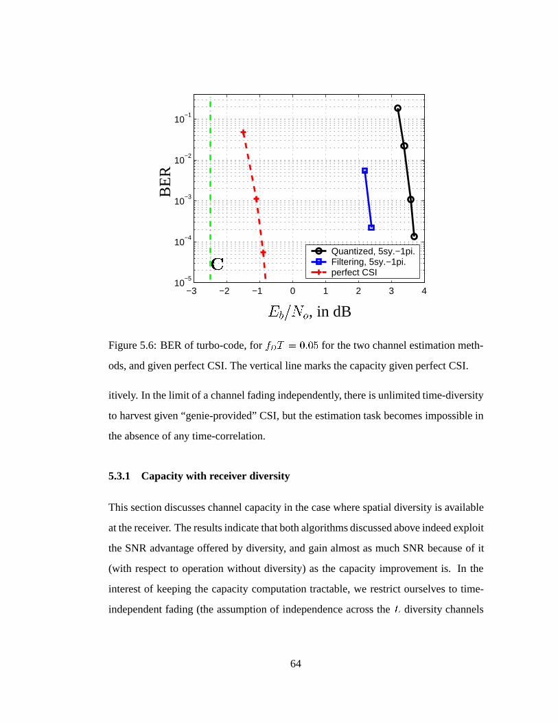
−3 −2 −1 0 1 2 3 410
−5
10−4
10−3
10−2
10−1
Quantized, 5sy.−1pi.Filtering, 5sy.−1pi.perfect CSI
BE
R
C
Eb=N
o, in dB
Figure 5.6: BER of turbo-code, for fDT = 0:05 for the two channel estimation meth-
ods, and given perfect CSI. The vertical line marks the capacity given perfect CSI.
itively. In the limit of a channel fading independently, there is unlimited time-diversity
to harvest given “genie-provided” CSI, but the estimation task becomes impossible in
the absence of any time-correlation.
5.3.1 Capacity with receiver diversity
This section discusses channel capacity in the case where spatial diversity is available
at the receiver. The results indicate that both algorithms discussed above indeed exploit
the SNR advantage offered by diversity, and gain almost as much SNR because of it
(with respect to operation without diversity) as the capacity improvement is. In the
interest of keeping the capacity computation tractable, we restrict ourselves to time-
independent fading (the assumption of independence across the L diversity channels
64
always remains) and also assume perfect knowledge of the fading gains at the receiver.
Specifically, consider L-branch diversity reception in flat Rayleigh fading, where
the received sample yi at each branch is:
yi = ai � x + ni; i = 1; : : : ; L; (5.28)
and denote the SNR as � = PxNo
, where Px is the average transmitted power of the
constellation point x. Then, collecting all received values into a vector of length L:
y = a � x + n; (5.29)
where all vectors a and n are assumed independent of each other and in time. The
capacity of this vector channel, when there is no time constraint and given perfect
channel knowledge at the receiver, is given by (see [2]):
CL =
Zlog2(1 + � aa�)Pa(a)da; (5.30)
where Pa is the distribution of the fading vector a. For instance, in the case of no
fading (L-branch AWGN diversity) where a = 1L always, we have that:
CAWGNL = log2(1 + �L); (5.31)
in other words the intuitively pleasing result that the AWGN capacity with L diversity
branches is the same as if the receiver has only one antenna, but the transmitter uses L
times more power. In the specific case of L = 2, the SNR gain from diversity is 3 dB.
In Rayleigh fading, where each element (fading scale factor) ai in the vector a is
a zero-mean, unit variance complex Gaussian random variable —i.e. ai � NC (0; 1)—
then it is expected that the SNR advantage due to diversity will be greater than 3 dB
for L = 2, because of the “sphere-hardening” phenomenon. In other words, the L-fold
receiver diversity helps in a dual fashion: it captures more of the transmitter power and
65
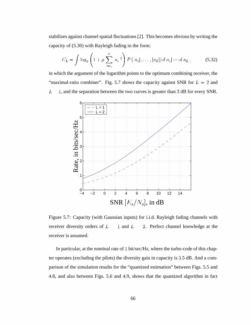
stabilizes against channel spatial fluctuations [2]. This becomes obvious by writing the
capacity of (5.30) with Rayleigh fading in the form:
CL =
Zlog2
1 + �
LXi=1
jaij2!P (ja1j; : : : ; jaLj) dja1j � � �djaLj; (5.32)
in which the argument of the logarithm points to the optimum combining receiver, the
“maximal-ratio combiner”. Fig. 5.7 shows the capacity against SNR for L = 2 and
L = 1, and the separation between the two curves is greater than 3 dB for every SNR.
−4 −2 0 2 4 6 8 10 12 140
1
2
3
4
5
6L = 1L = 2
SNR [Es=N
o], in dB
Rat
e,in
bits
/sec
/Hz
Figure 5.7: Capacity (with Gaussian inputs) for i.i.d. Rayleigh fading channels with
receiver diversity orders of L = 1 and L = 2. Perfect channel knowledge at the
receiver is assumed.
In particular, at the nominal rate of 1 bit/sec/Hz, where the turbo-code of this chap-
ter operates (excluding the pilots) the diversity gain in capacity is 3:5 dB. And a com-
parison of the simulation results for the “quantized estimation” between Figs. 5.5 and
4.8, and also between Figs. 5.6 and 4.9, shows that the quantized algorithm in fact
66
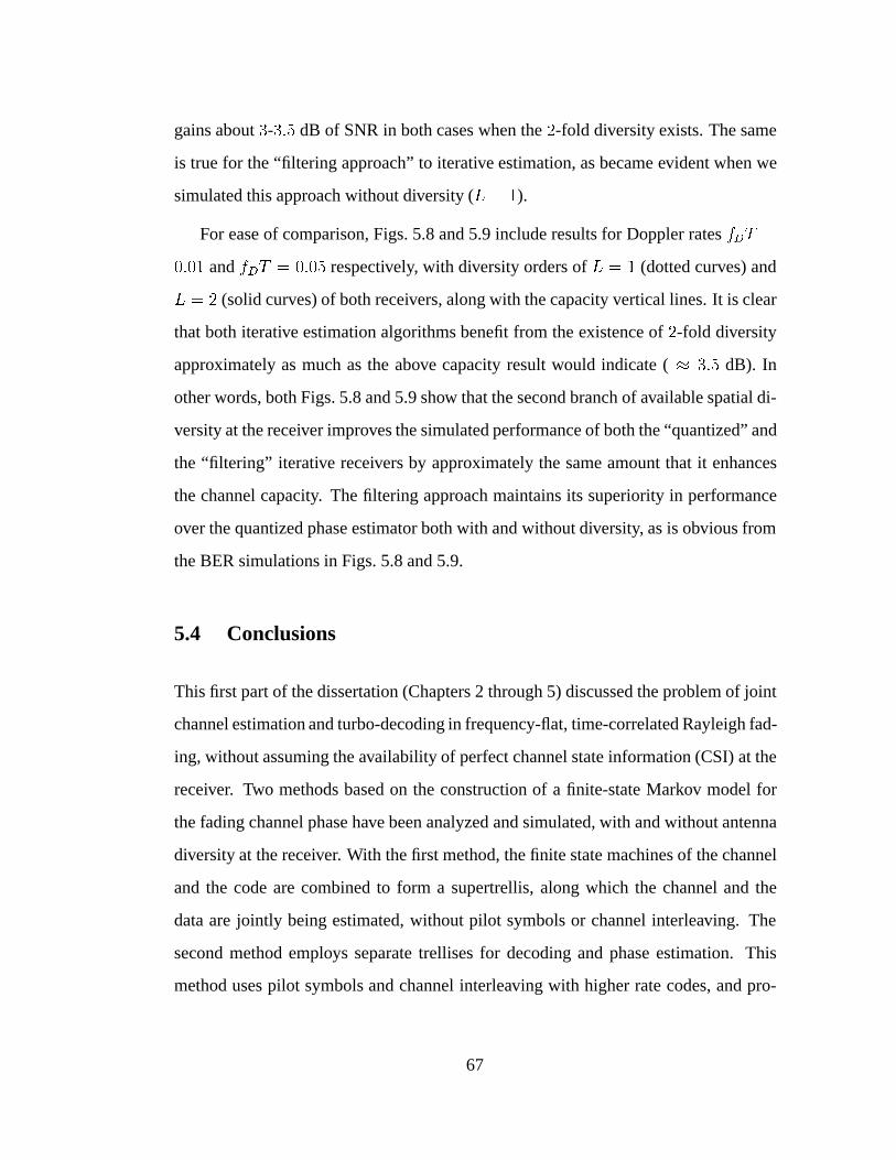
gains about 3-3:5 dB of SNR in both cases when the 2-fold diversity exists. The same
is true for the “filtering approach” to iterative estimation, as became evident when we
simulated this approach without diversity (L = 1).
For ease of comparison, Figs. 5.8 and 5.9 include results for Doppler rates fDT =
0:01 and fDT = 0:05 respectively, with diversity orders of L = 1 (dotted curves) and
L = 2 (solid curves) of both receivers, along with the capacity vertical lines. It is clear
that both iterative estimation algorithms benefit from the existence of 2-fold diversity
approximately as much as the above capacity result would indicate ( � 3:5 dB). In
other words, both Figs. 5.8 and 5.9 show that the second branch of available spatial di-
versity at the receiver improves the simulated performance of both the “quantized” and
the “filtering” iterative receivers by approximately the same amount that it enhances
the channel capacity. The filtering approach maintains its superiority in performance
over the quantized phase estimator both with and without diversity, as is obvious from
the BER simulations in Figs. 5.8 and 5.9.
5.4 Conclusions
This first part of the dissertation (Chapters 2 through 5) discussed the problem of joint
channel estimation and turbo-decoding in frequency-flat, time-correlated Rayleigh fad-
ing, without assuming the availability of perfect channel state information (CSI) at the
receiver. Two methods based on the construction of a finite-state Markov model for
the fading channel phase have been analyzed and simulated, with and without antenna
diversity at the receiver. With the first method, the finite state machines of the channel
and the code are combined to form a supertrellis, along which the channel and the
data are jointly being estimated, without pilot symbols or channel interleaving. The
second method employs separate trellises for decoding and phase estimation. This
method uses pilot symbols and channel interleaving with higher rate codes, and pro-
67

vides good performance approaching a sequence of upper bounds to capacity with
reasonable complexity. The estimation of channel phase and data is done jointly, on
the supertrellis or on the separate trellises, via the Forward-Backward algorithm. Also,
generalized iterative Wiener filtering is considered as an alternative for estimation, and
shown to achieve good performance with high-rate trellis turbo-codes.
68
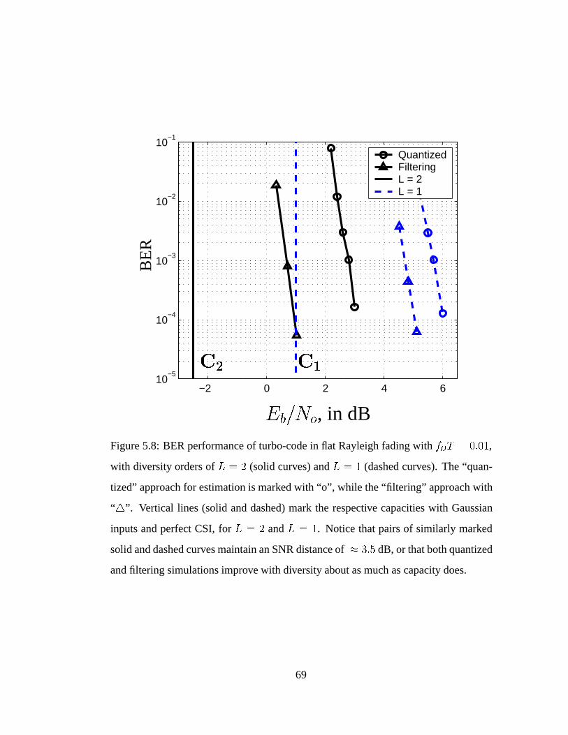
−2 0 2 4 610
−5
10−4
10−3
10−2
10−1
QuantizedFilteringL = 2 L = 1
C2 C1
Eb=No, in dB
BE
R
Figure 5.8: BER performance of turbo-code in flat Rayleigh fading with fDT = 0:01,
with diversity orders of L = 2 (solid curves) and L = 1 (dashed curves). The “quan-
tized” approach for estimation is marked with “o”, while the “filtering” approach with
“4”. Vertical lines (solid and dashed) mark the respective capacities with Gaussian
inputs and perfect CSI, for L = 2 and L = 1. Notice that pairs of similarly marked
solid and dashed curves maintain an SNR distance of � 3:5 dB, or that both quantized
and filtering simulations improve with diversity about as much as capacity does.
69
−2 0 2 4 6 810
−5
10−4
10−3
10−2
10−1
QuantizedFilteringL = 2 L = 1
C2 C1
Eb=No, in dB
BE
R
Figure 5.9: BER performance of turbo-code in flat Rayleigh fading with fDT = 0:05.
Naming conventions are the same as in Fig. 5.8. Again, notice that the second branch
of diversity improves the simulations (dashed to solid curve with the same marker) by
about as much as it improves the capacity (dashed to solid vertical line).
70
Part II
MIMO SYSTEMS IN
FREQUENCY-SELECTIVE FADING
71
CHAPTER 6
MIMO Frequency-Selective Channel
6.1 Introduction
This second part of the dissertation addresses the problem of channel tracking and
equalization for multi-input multi-output (MIMO) time-variant frequency-selective
channels. These channels model the corrupting effects of inter-symbol interference
(ISI), co-channel interference (CCI), and noise. The frequency selectivity of the chan-
nel arises in a MIMO (nT ; nR) wireless system, where nT � 1 is the number of trans-
mitter antennas and nR � 1 is the number of receiver antennas, as a result of relatively
high transmission rates, whereby the transmission bandwidth exceeds the coherence
bandwidth of the channel. Regarding the time-variant nature of the MIMO frequency-
selective channel, this dissertation considers it to be significant within a packet of data,
hence the need for channel tracking arises in order for the equalization to be effective.
In other words, this and the next chapter consider the MIMO transmission problem for
the important area of operation, where the transmission rate is high enough to generate
resolvable multipath at the receiver, and at the same time the transmitted packet is long
enough (or the transmission rate slow enough) to render an assumption of constant
channel in every data burst inaccurate.
Most of the discussion of MIMO transmission in this and the next chapter is gen-
eral enough to cover both the case of nT independent users with one antenna each
(which can be thought of as the multi-user detection problem, for instance in wideband
72
multiple access systems [35], [36]), as well as the case of one user with coordinated
transmissions through nT antennas for higher data rate (which is akin to the systems of
[2], [37]). This difference clearly has a big effect upon the choice of appropriate cod-
ing mechanisms for the MIMO system, discussed in Chapter 7, but does not affect the
tracking procedure. For MIMO tracking we use a Kalman filter, aided by staggered
decisions from a finite-length MMSE-DFE, which performs the task of equalization
and separation of the sources.
An excellent review article [38] by Qureshi discusses adaptive equalization of a
single-input single-output (SISO) dispersive channel (nT = nR = 1). For a fading
SISO channel with ISI, a comprehensive review of the extensive research is [39]. In
[40] we present a special case of the results in this dissertation, applicable to the SISO
scenario. For array measurements at the receiver (nT = 1; nR > 1) an adaptive ap-
proach based on per-survivor-processing (PSP) is explored in [41]. The same case
(nT = 1; nR > 1) but for flat fading (no ISI) was treated from the estimation and
coding perspective in Chapter 5. But when more transmitters are sharing the band-
width, there are two broad classes of techniques to combat co-channel interference
(CCI) at the receiver. One is to suppress interference, possibly in an adaptive fashion,
as in [42]. Another strategy is to decode all nT data sequences simultaneously (e.g.
[36]), possibly with a blind/adaptive approach [43]. The method we demonstrate in the
next chapter embraces the second paradigm, with a few key differences from previous
approaches.
First, we adopt the design of a finite-length MMSE-DFE from [44] for practical
implementation. Then, we consider the channel taps to have significant time-variation
from symbol to symbol, but with largely invariant specular mean and Doppler, which
can be identified during a training phase. After that, in tracking mode, the Kalman
filter and this finite MIMO DFE cooperate to adapt to the rapid channel variations.
73
It should be noted that, at least for the single-user (SISO) channel, Kalman-based
estimation methods are quite common in the literature (e.g., [45] uses the extended
Kalman filter to track a channel with unknown delays). Also, in [46] the Kalman
approach is used to formulate extended forms of the Recursive Least-Squares (RLS)
algorithm, and the tracking superiority of those is demonstrated compared to the stan-
dard RLS and Least Mean-Squares (LMS) algorithms.
In Chapter 7 we use a Kalman filter to track the time-variation of the MIMO chan-
nel taps. These taps are typically modeled as mutually uncorrelated circular complex
Gaussian random processes, having locally constant means, due to large scale path
loss, reflections and shadowing effects, as discussed in section 6.2. We assume the tap
means known from a preceding training phase, and concentrate on tracking their time-
variant part, which has autocorrelation properties corresponding to the wide-sense sta-
tionary and uncorrelated scattering “WSSUS” model of Bello [47]. If the tap means
are zero, the channel is said to introduce Rayleigh fading (worst case), while a non-
zero mean tap corresponds to Ricean fading. The Kalman channel estimator is aided
by previous hard decisions about the transmitted symbols from all users, produced by
the MIMO equalizer.
Assuming perfect knowledge of the MIMO channel, the optimum receiver is a
maximum likelihood sequence estimator (MLSE), but its complexity is prohibitive,
even for low order channels with a small number of inputs and outputs. In Chap-
ter 7 we use the MIMO finite-length minimum-mean-squared-error decision-feedback
equalizer (MMSE-DFE), developed in [44] and optimized for decision delay � � 0.
The choice of � > 0 improves performance for a wide range of channels, as shown
in [40] for the single-user channel. However, this delay poses the problem of channel
prediction when combined with the Kalman tracking procedure mentioned above, be-
cause there is a time gap of � between channel estimates produced by the Kalman filter
74
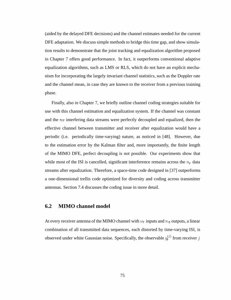
(aided by the delayed DFE decisions) and the channel estimates needed for the current
DFE adaptation. We discuss simple methods to bridge this time gap, and show simula-
tion results to demonstrate that the joint tracking and equalization algorithm proposed
in Chapter 7 offers good performance. In fact, it outperforms conventional adaptive
equalization algorithms, such as LMS or RLS, which do not have an explicit mecha-
nism for incorporating the largely invariant channel statistics, such as the Doppler rate
and the channel mean, in case they are known to the receiver from a previous training
phase.
Finally, also in Chapter 7, we briefly outline channel coding strategies suitable for
use with this channel estimation and equalization system. If the channel was constant
and the nT interfering data streams were perfectly decoupled and equalized, then the
effective channel between transmitter and receiver after equalization would have a
periodic (i.e. periodically time-varying) nature, as noticed in [48]. However, due
to the estimation error by the Kalman filter and, more importantly, the finite length
of the MIMO DFE, perfect decoupling is not possible. Our experiments show that
while most of the ISI is cancelled, significant interference remains across the nT data
streams after equalization. Therefore, a space-time code designed in [37] outperforms
a one-dimensional trellis code optimized for diversity and coding across transmitter
antennas. Section 7.4 discusses the coding issue in more detail.
6.2 MIMO channel model
At every receiver antenna of the MIMO channel with nT inputs and nR outputs, a linear
combination of all transmitted data sequences, each distorted by time-varying ISI, is
observed under white Gaussian noise. Specifically, the observable y(j)t from receiver j
75
(with j = 1; : : : ; nR) at time t is:
y
(j)t =
nTXi=1
�(i;j)Xm=0
c(i;j)m (t) x
(i)t�m + v
(j)t (6.1)
where c(i;j)m is the mth tap of the impulse response of order �(i;j) between the ith input
x(i) and the jth output y(j) of the MIMO channel. The complex baseband constellation
point x(i)t�m is transmitted by the ith user at time t �m, and v
(j)t is the complex noise
sample at the jth receiver. In essence, there exist a total of nTnR interfering, time-
varying ISI channels c(i;j)(t) (see Fig. 6.1 for a (2; 2) system):
c(i;j)(t) =hc
(i;j)0 (t) c
(i;j)1 (t) : : : c
(i;j)
�(i;j)(t)i
(6.2)
and each of their taps can be written as:
c(i;j)m (t) = �c(i;j)m + h
(i;j)m (t); m = 0; : : : ; � (6.3)
where we define � = maxi;j �(i;j), and set c(i;j)m (t) = 0 for m > �
(i;j).
c(2;1)(t)
x(1)t
x(2)t
c(2;2)(t)
c(1;2)(t)
y(1)t
y(2)t
c(1;1)(t)
Figure 6.1: The interfering ISI channels in a (2; 2) MIMO system.
The time-varying part h(i;j)m (t) of each tap in (6.3) is a zero-mean, wide-sense-
stationary complex Gaussian process, uncorrelated with any other h(i0;j0)
m0 (t), and has
time-autocorrelation properties governed by the Doppler rate fDT , (T is the baud du-
ration) as in [17]:
Efh(i;j)m (t1)[h(i;j)m (t2)]
�g�Jo�2�f
(i;j;m)
D T jt1 � t2j�
(6.4)
76
where Jo(�) is the zero-order Bessel function of the first kind. Notice that each of
the nTnR(� + 1) taps varies independently (although this will not be essential in our
development) and can have a different Doppler rate. More importantly, the autocorre-
lation functions are non-rational, hence no ARMA model is an exact representation of
the time evolution of the channel taps. However, only the first few correlation terms
(for small jt1 � t2j) are important for the design of any receiver. Thus, even low order
autoregressive models, or even a simple Gauss-Markov model, can capture most of
the channel tap dynamics and lead to effective tracking algorithms, as demonstrated
below.
Analogous to a Single-Input, Single-Output (SISO) system with nT = nR = 1, we
can write the MIMO channel input-output relationship in vector form as a matrix FIR
filter. By collecting the outputs y(j)t of (6.1) from all receiver antennas at time t into a
nR-dimensional column vector yt:
yt =
�Xm=0
Cm(t)xt�m + vt; (6.5)
where yt and vt are column vectors of length nR, xt�m are column vectors of length
nT , and Cm(t) are nR � nT matrix channel taps (instead of the scalar SISO taps).
Each of the matrices Cm(t), m = 0; : : : ; � contains the tap c(i;j)m (t) of (6.1) and (6.3)
in its (j; i)th position. This formulation of the MIMO channel (6.5) is useful in the
DFE design of section 7.1.2, but for the purpose of MIMO channel tracking via the
Kalman filter, presented in section 7.1.1, we will need an alternative notation for the
input-output relationship, of the form:
yt = Xt � ct + vt; (6.6)
where the nR � nRnT (� + 1) data matrix Xt is a “wide” matrix with the transmitted
symbols repeated diagonally, according to the Kronecker product:
Xt=hx
(1)t : : : x
(nT )t x
(1)t�1: : : x
(nT )t�1 : : : x
(1)t�� : : : x
(nT )t��
i InR (6.7)
77
and ct is a long vector of length nTnR(� + 1) containing all the channel taps at time t,
ct = �c+ ht:
ct =hc
(1;1)0 (t) : : : c
(1;nR)0 (t) : : : c
(nT ;1)0 (t) : : : c
(nT ;nR)0 (t) : : :
c(1;1)� (t) : : : c(1;nR)� (t) : : : c(nT ;1)� (t) : : : c(nT ;nR)� (t)
�T: (6.8)
With this setup, the channel is a complex Gaussian vector process ct with dimensions
(nTnR(� + 1))� 1, which has a constant mean vector �c. The time-variant part of the
channel is the vector process fhtg. According to the WSSUS model of Bello [47],
all the channel taps are independent, namely all the entries of vector ht vary indepen-
dently, according to the autocorrelation model of (6.4). If we let index k enumerate all
the taps k = 1; : : : ; nTnR(� + 1), and denote f (k)D = f
(i;j;m)
D the Doppler of the mth
tap of the channel from input i to output j, then the normalized spectrum for each tap
fh(k)t g is:
Sk(f)=
8>>>>><>>>>>:
1
�f
(k)
D T
1vuut1�
f
f
(k)
D T
!2; jf j < f
(k)
D T
0; otherwise
(6.9)
Exact modeling of the vector process fhtg with an autoregressive (AR) model is
impossible. For implementation of a Kalman filter, we approximate the MIMO channel
variation fhtg with the following multichannel AR process of order p, as done in [49]
for nT = nR = 1:
ht =
pXl=1
A(l)ht�l +Gwt; (6.10)
where wt is a zero-mean i.i.d. circular complex Gaussian vector process with correla-
tion matricesRww(j) for every lag j given byRww(j) = Efwtw�t+jg = InT nR(�+1)�(j).
Due to the WSSUS assumption, the matrices A(l), l = 1; : : : ; p and G of the model
(6.10) must be diagonal. For the selection of their diagonal entries, various criteria of
78
optimality can be adopted, such that the AR(p) model of (6.10) would be a “best-fit”
to the true channel autocorrelation of (6.4). One such criterion can be to require the
process (6.10) to be such that 90% of the energy spectrum of each tap is contained in
the frequency range jf j < f
(k)
D T , as indicated by (6.9).
For simplicity we adopt a first-order AR model (p = 1) and denote F = A(1). So,
(6.10) becomes:
ht = Fht�1 +Gwt (6.11)
Then we fix the diagonal entries of matricesF andG (call them fk and gk respectively)
to capture the most essential parts of the channel variation, namely how “fast” and how
“much” the time-varying part h(k) of each channel tap varies with respect to the mean
of that tap �ck. The speed of variation is determined by the Doppler, or equivalently by
the relative velocity between the nT antennas of the transmitter and the nR antennas
of the receiver. At least for the scenario of coordinated transmission, the assumption
of equal Doppler rates f (k)D T = fDT , k = 1; : : : ; nTnR(� + 1) makes intuitive sense,
so we adopt it in the simulations, although the algorithm derivation certainly does not
rely on that. The diagonal entries of F are all fk = f = Jo (2�fDT ), and this choice
sets the autocorrelation of the taps modeled by (6.11) to equal the true autocorrelation
at unit lag. Obviously, larger Doppler rate fDT implies smaller fk = f , hence faster
channel variation.
Having fixed the rate of channel variation via F, the magnitude of variation of the
kth tap is then controlled by the diagonal entries gk of G, since the power of the time-
variant part of each tap is Ejh(k)j2 =g2k
1�f2 , from (6.11). The amount of variation of
each tap with respect to the mean is expressed by the “specular-to-diffuse power ratio”
Kk, as follows:
Kkdef= 10 log
� j�ckj2Efjh(k)j2g
�=10 log
� j�ckj2g2k=(1� f
2k )
�(6.12)
79
The ratio Kk indicates the ratio of power of the kth mean channel tap to the mean-
squared power of the random, time-variant part of that tap, analogous to the Ricean
factor defined in the wireless channel literature. Clearly, K = �1 dB corresponds
to Rayleigh taps, while large positive values of K in dB represent almost no channel
variation at all. In the simulations of Chapter 7, although again it is arbitrary, we
choose equal values of Kk = K for all the taps.
Although higher order models than (6.11) can be constructed for larger p, it turns
out that this simple first-order approximation is enough to model the channel dynamics
to the extent necessary for a receiver to operate. For perspective, in a 2:4 GHz trans-
mission with baud rate of 20 KHz and Doppler frequency fD = 200 Hz (corresponding
to vehicular velocity of 90 Km/h or 56 mph), then fDT = 0:01 and fk = 0:999. Also,
a value of K = 6 dB implies that the average power of each tap variation is one-fourth
of the constant mean tap value.
For the SISO case (i.e. nT = 1; nR = 1) a useful method to obtain the sequence
of matrices A(l); l = 1; : : : ; p during a training mode is provided in [49], via higher-
(than-second)-order statistics (HOS). Their method is effective and requires only rea-
sonable assumptions about the transmitted sequence and the noise. An analogous train-
ing method can be adopted for general MIMO channels. But the way we formulated
the AR(1) model of (6.11) here, the information needed to construct the model is only
the channel mean �c, the Doppler rates, the ratios Kk and the noise variance. Hence, we
assume that these quantities are known from a training phase, and focus on decision-
aided tracking of the channel for relatively long time spans, without retraining.
80
CHAPTER 7
Receiver Structure and Performance
7.1 Receiver structure
The receiver uses a Kalman filter to track the channel and a DFE to equalize it. The
Kalman filter assumes that the DFE hard decisions are correct and uses them to es-
timate the next channel value, while the DFE assumes correct Kalman filter channel
estimates, and uses them in turn to equalize the channel. In general, the optimum de-
cision delay � � 0 can be determined analytically given a channel (see [44]). For a
wide range of channels (including, but not limited to, non-minimum-phase channels),
it turns out that a DFE producing decisions with � > 0 is optimal. Even for the few
channels where � = 0 is best, it doesn’t degrade performance to use a DFE with
� > 0, provided there are enough taps in the feedforward and feedback filters. Thus,
it makes sense, particularly for time-varying channels like the ones treated here, to use
decision delays � > 0.
But when � > 0, a time gap is created. At time t, when the last received vector
is yt, the DFE produces the hard-decision xt��. The staggered decisions cause the
Kalman filter to operate with delay, that is, operate at time t � �, since it only has
available hard decisions from the DFE up to then. However, the DFE design still needs
channel estimates up to time t. Thus the receiver needs to use channel prediction to
bridge the time gap between the Kalman channel estimation and the channel estimates
needed for the current DFE adaptation.
81
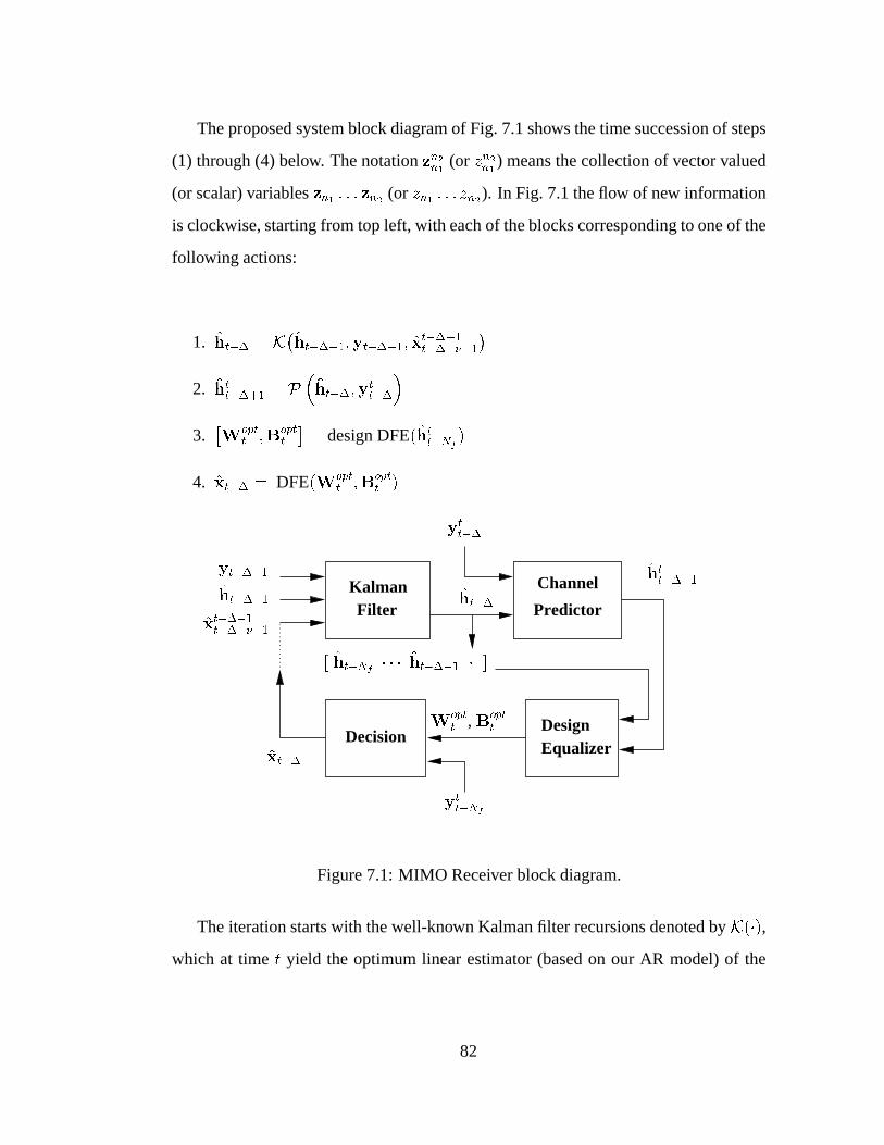
The proposed system block diagram of Fig. 7.1 shows the time succession of steps
(1) through (4) below. The notation zn2n1 (or zn2n1 ) means the collection of vector valued
(or scalar) variables zn1 : : : zn2 (or zn1 : : : zn2). In Fig. 7.1 the flow of new information
is clockwise, starting from top left, with each of the blocks corresponding to one of the
following actions:
1. ht�� = K�ht���1;yt���1; xt���1t�����1
�2. htt��+1 = P
�ht��;y
tt��
�3.�W
optt ;B
optt
�= design DFE(htt�Nf
)
4. xt�� = DFE(Woptt ;B
optt )
DesignEqualizer
Decision
KalmanFilter
Channel
Predictor
Wopt
t, Bopt
t
ytt��
ytt�Nf
xt��
htt��+1
ht��
[ ht�Nf� � � ht���1 � ]
ht���1
yt���1
xt���1t�����1
Figure 7.1: MIMO Receiver block diagram.
The iteration starts with the well-known Kalman filter recursions denoted by K(�),which at time t yield the optimum linear estimator (based on our AR model) of the
82
time-varying part of the channel ht�� as it was at time t��. For that, the Kalman filter
relies on the (assumed reliable) DFE decisions xt���1; : : : ; xt�����1, the received
vector yt���1 and the previously estimated channel vector ht���1. In the second step,
P(�) denotes a predictor that may exploit the additional received vectors yt; : : :yt��,
along with the last Kalman estimate ht�� to compute the sequence of � predicted
channels ht; : : : ; ht��+1.
Those � predicted channels, along with the Nf �� most recent channel estimates
from the Kalman filter, are used by the DFE design module (see Sect. 7.1.2) to design
the optimum feedforward matrix filter, Woptt , and the feedback matrix filter, Bopt
t of
an MMSE DFE. Finally, the newly designed DFE decodes one more nT -dimensional
symbol xt��, which is added to the collection of past (assumed reliable) decisions,
which will help the Kalman filter make a new channel estimate ht��+1 at the next
iteration, taking place at time instant t+1. In the following subsections we look at the
implementation of the two main receiver modules in greater detail.
7.1.1 Kalman tracking and channel prediction
For simplicity, we limit our discussion to the AR(1) channel model of (6.11), but the
extension to higher order AR models is straightforward. The channel at time t has
a constant (assumed known) mean �c and a zero-mean time-varying part ht, which
follows the AR(1) model:
ht+1 = Fht +Gwt: (7.1)
At time t, the (zero-mean) received vector yt is given by:
yt = Xt � (�c+ ht) + vt: (7.2)
Assuming the matrices F and G and the mean channel vector �c are known from a
preceding training phase, and assuming the matrix of the most recent available deci-
83
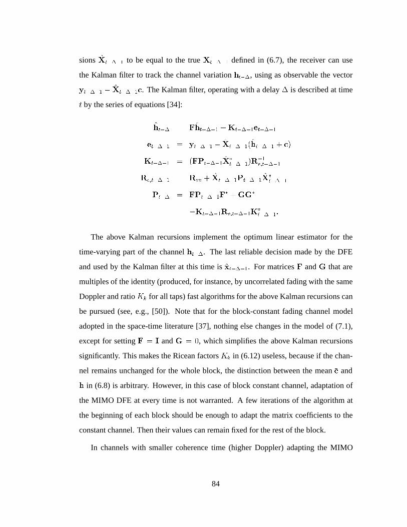
sions Xt���1 to be equal to the true Xt���1 defined in (6.7), the receiver can use
the Kalman filter to track the channel variation ht��, using as observable the vector
yt���1 � Xt���1�c. The Kalman filter, operating with a delay � is described at time
t by the series of equations [34]:
ht�� = Fht���1 +Kt���1et���1
et���1 = yt���1 � Xt���1(ht���1 + �c)
Kt���1 = (FPt���1X�t���1)R
�1e;t���1
Re;t���1 = Rvv + Xt���1Pt���1X�t���1
Pt�� = FPt���1F� +GG�
�Kt���1Re;t���1K�t���1:
The above Kalman recursions implement the optimum linear estimator for the
time-varying part of the channel ht��. The last reliable decision made by the DFE
and used by the Kalman filter at this time is xt���1. For matrices F and G that are
multiples of the identity (produced, for instance, by uncorrelated fading with the same
Doppler and ratio Kk for all taps) fast algorithms for the above Kalman recursions can
be pursued (see, e.g., [50]). Note that for the block-constant fading channel model
adopted in the space-time literature [37], nothing else changes in the model of (7.1),
except for setting F = I and G = 0, which simplifies the above Kalman recursions
significantly. This makes the Ricean factors Kk in (6.12) useless, because if the chan-
nel remains unchanged for the whole block, the distinction between the mean �c and
h in (6.8) is arbitrary. However, in this case of block constant channel, adaptation of
the MIMO DFE at every time is not warranted. A few iterations of the algorithm at
the beginning of each block should be enough to adapt the matrix coefficients to the
constant channel. Then their values can remain fixed for the rest of the block.
In channels with smaller coherence time (higher Doppler) adapting the MIMO
84
DFE every time instant improves performance. For designing the DFE at time t (step
3), the Nf most recent channel estimates are needed, where Nf is the order of the
matrix feedforward filter Wopt of the DFE. Up to time t � � channel estimates are
available from the Kalman filter. But the last� channel vectors ht; : : : ; ht��+1 have to
be predicted. The implementation of the prediction depends upon the SNR of operation
and how fast the channel varies. For the block-constant channel or a very slowly
varying one, the simplest choice is to assume that the channel remains constant over
� sampling periods, that is:
ht = ht�1 = � � � = ht�� (7.3)
where ht�� is already provided by the Kalman filter.
More generally, the optimal linear predictions, given that the channel follows the
AR(1) model of (7.1), but ignoring the additional received vectors yt; : : : ;yt�� are:
ht = F�ht��; : : : ; ht��+1 = Fht�� (7.4)
where again ht�� is the last Kalman channel estimate.
The received vectors yt; : : : ;yt��, which are also available, can be used to im-
prove the prediction for a fast varying channel at high SNR. For example, one could
formulate and optimize least-squares cost functions J(h), forcing the predicted chan-
nel vectors hk; k = t; : : : ; t � � + 1 to the vicinity of the values of (7.4), weighted
by how well a certain hk “justifies” the received vectors yt; : : : ;yt�� (see [40]). We
do not pursue this prediction avenue in this chapter, and all simulations are done using
(7.4) for channel prediction.
7.1.2 DFE design
The design of the optimum MMSE feedforward and feedback matrix filters Wopt and
Bopt of lengths Nf and Nb matrix taps respectively, as well as the optimum selection
85
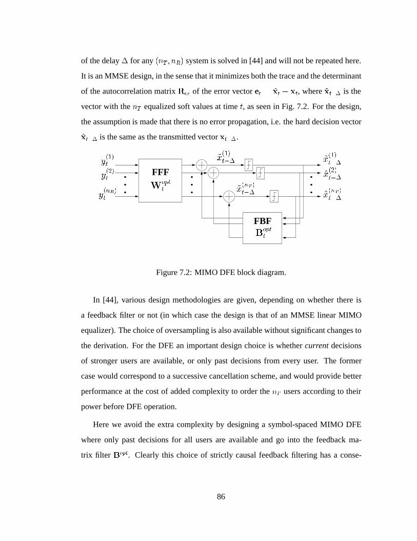
of the delay � for any (nT ; nR) system is solved in [44] and will not be repeated here.
It is an MMSE design, in the sense that it minimizes both the trace and the determinant
of the autocorrelation matrix Ree of the error vector et = ~xt � xt, where ~xt�� is the
vector with the nT equalized soft values at time t, as seen in Fig. 7.2. For the design,
the assumption is made that there is no error propagation, i.e. the hard decision vector
xt�� is the same as the transmitted vector xt��.
~x(nT )
t��
FBFB
opt
t
~x(1)
t��
Wopt
t
FFFy(1)t
y(2)t
y(nR)t
x(nT )
t��
x(1)
t��
x(2)
t��
Figure 7.2: MIMO DFE block diagram.
In [44], various design methodologies are given, depending on whether there is
a feedback filter or not (in which case the design is that of an MMSE linear MIMO
equalizer). The choice of oversampling is also available without significant changes to
the derivation. For the DFE an important design choice is whether current decisions
of stronger users are available, or only past decisions from every user. The former
case would correspond to a successive cancellation scheme, and would provide better
performance at the cost of added complexity to order the nT users according to their
power before DFE operation.
Here we avoid the extra complexity by designing a symbol-spaced MIMO DFE
where only past decisions for all users are available and go into the feedback ma-
trix filter Bopt. Clearly this choice of strictly causal feedback filtering has a conse-
86

quence: while it permits almost perfect cancellation of the ISI and cross-ISI, it does
not completely suppress residual cross-coupling. In other words, the ith entry ~x
(i)t
of the equalized vector ~xt is almost devoid of the corrupting presence of all x(j)t�k,
k 6= 0; j = 1; : : : ; nT , but the presence of current other symbols x(j)t , j 6= i, in it is
nulled somewhat less effectively.
We do not replicate the equations for optimum design of Wopt and Bopt here.
Suffice it to say that an essential part of the DFE design at every time instant t is the
formulation of the nRNf � nT (Nf + �) block pre-windowed channel matrix H:
H=
26666664Ct
0 � � � Ct� 0 � � � 0
0 Ct�10 � � � Ct�1
� 0 � � �...
...
0 � � � 0 Ct�Nf+1
0 � � � Ct�Nf+1�
37777775 (7.5)
where Ckm; m = 0; 1; : : : ; �, k = t; t � 1; : : : ; t � Nf + 1 are the estimates of
the nR � nT channel matrices Cm(k) in (6.5). It is obvious that constructing H
of (7.5) merely involves adding the constant part �c to the long vector estimates hk,
k = t; t � 1; : : : ; t � Nf + 1 of the time-varying part of the channel (some of which
are estimated via the Kalman filter and some are predicted), and then rearranging the
resulting long vectors into the dimensions specified by Eq. (6.5). After the matrix
H of (7.5) has been formed, the MIMO DFE design procedure described in [44] is
straightforward, and also provides the correlation matrix Ree of the error vector as a
by-product. Fast Cholesky factorization improves the computational efficiency of this
finite-length MIMO DFE design, playing a role parallel to that of spectral factorization
for matrix filters of infinite length.
87

7.2 Baseline adaptive systems
In this section we outline conventional adaptive algorithms for the DFE, such as LMS
and RLS for the case of nT transmitters and nR receivers. These adaptation mech-
anisms, unlike the Kalman-aided DFE presented above, do not estimate the channel
explicitly. Instead, they adapt the DFE matrix taps, based on observed symbols from
the time-variant channel, and hard decisions from the equalizer. LMS and RLS will
serve as baseline systems, the performance of which will be compared to the Kalman-
aided DFE through simulations in the next section. For both algorithms, consider
the concatenation of the nT � nRNf matrix FF filter and the nT � nTNb matrix FB
filter of the DFE into an nT � (nRNf + nTNb) equalizer filter Q = [W B]. At
time t, this equalizer filter Qt operates on the column “regressor” vector ut of length
nRNf + nTNb:
ut = [yTt : : :yTt�Nf+1 x
Tt���1 : : : x
Tt���Nb
]T (7.6)
The operation produces a vector ~xt�� of nT soft values, which are then fed to nT
slicers, as in Fig. 7.2, producing a vector of hard decisions xt��. Under the MMSE
criterion, each row qi; i = 1; : : : ; nT of the equalizer Qt is responsible for the mini-
mization of the cost function:
J(qi) = jx(i)t�� � qi � uj2 = jx(i)t�� � qi � uj2; i = 1; : : : ; nT ; (7.7)
with the high-SNR assumption of no decision errors. In the absence of knowledge
of the correlations Rx(i)u = Ex(i)u� and Ru = Euu�, we can use the corresponding
instantaneous approximations x(i)u� and uu� in their place. This leads to the following
LMS recursions, which iteratively approximate the least-mean-square solution (see
[34]) separately for i = 1; : : : ; nT :
qi(t) = qi(t� 1) + �[x(i)
t�� � qi(t� 1) � ut]u�t : (7.8)
88
Those nT simultaneous LMS recursions for the rows qi of Q can be combined into
one, for the entire DFE Q:
MIMO LMS: Qt = Qt�1 + �[xt�� �Qt�1 � ut]u�t : (7.9)
Similarly, considering nT parallel RLS adaptations for each row, and this time using
instantaneous approximations for the necessary correlation matrices in a Newton re-
cursion (see [34]), we get:
qi(t) = qi(t� 1) +hx
(i)
t�� � qi(t� 1) � utiu�tPt;
for i = 1; : : : ; nT ; with :
Pt = ��1 �
�Pt�1 � �
�1Pt�1utu
�tPt�1
1 + ��1u�tPt�1ut
�which, again, can be combined into one matrix recursion for Qt:
MIMO RLS:Qt = Qt�1 + [xt�� �Qt�1 � ut]u�tPt
Pt = ��1 ��Pt�1 � �
�1Pt�1utu
�tPt�1
1 + ��1u�tPt�1ut
� (7.10)
with initial condition P�1 = �oI and 0� � � 1.
Note that the recursive adaptation of (7.10) above is known to not only be an ap-
proximation to Newton’s method with instantaneous values in the places of unknown
auto- and cross-correlations, but also to be the exact solution of a weighted, regularized
least-squares problem involving a block of observations and a single equalizer matrix
Q. In fact, with the obvious changes to accommodate the different dimensions of Q,
the RLS recursion of (7.10) with the update for Pt coming first, can easily be shown
to be exactly equivalent to the more compact RLS recursions given in [34, Chap. 10]
89
and [51, p. 569], with the update for Pt after the equalizer update:
MIMO RLS (II):
(t) =1
1 + ��1u�tPt�1ut
gt = ��1u�tPt�1 (t)
Qt = Qt�1 + [xt�� �Qt�1 � ut] � gtPt = �
�1 � [Pt�1 � Pt�1utgt]
(7.11)
7.3 Simulation results
In all simulations presented in this section we implemented the Kalman-aided MIMO
DFE algorithm outlined in section 7.1 and compared the performance of the system,
as measured by its symbol error rate (SER) when transmitting 4-PSK constellation
points through (2; 2) and single-user (i.e. (1; 1)) Ricean fading channels. We assumed
the channel mean to be known at the beginning of each block of N symbols per user
and tracked with the Kalman filter thereafter. For comparison purposes the plots in-
clude (dashed lines) the SER performance with the receiver having access to “genie-
provided” perfect channel information, as well as that of conventional adaptive receiver
algorithms, such as the LMS and RLS of section 7.2, admittedly less computationally
intensive than the tracking algorithm proposed in this chapter.
The SNR is set to be the same for both users (worst-case scenario, because having
one user stronger than others facilitates decoding of every user). Also, all nTnR mean
interfering channels of (6.2) are normalized jj�c(i;j)jj2 = 1, and all ratios Kk are chosen
equal to a single K. Thus, with �2v being the noise variance at each receiver, the SNR
plotted is the SNR of each interfering channel, neglecting co-channel interference:
SNR = 10 log1 + 10K=10
�2v
; (7.12)
since the input 4-PSK points are normalized to unit power. Clearly, for the (2; 2) ex-
ample, the above definition of SNR corresponds to 3 dB higher SNR (i.e. 10 lognT )
90
than that defined in space-time systems (see [2]), because we allocate unit power to
each transmitter antenna, thinking about individual uncoordinated users. For coordi-
nated transmission, to maintain a fair comparison with conventional (1; 1) systems,
input power must be split evenly among the nT transmitter antennas, which lowers the
SNR by 10 lognT dB.
In Fig. 7.3 the mean channels were the normalized versions of (1 + j)[1 0:8] and
(1 + j)[1 0:3] for the direct paths, and (1 + j)[1 � 0:8] and (1 + j)[1 � 0:5] for
the interfering paths, the Doppler rate was fDT = 0:01 (resulting in an AR(1) coef-
ficient f = 0:999) and the specular-to-diffuse power ratio was K = 6 dB. The indi-
cated symbol-error rate (SER) performance represents unsupervised channel tracking
for long blocks of N = 5000 symbols per user. The proposed Kalman-aided DFE
performs less than 1 dB from perfect channel knowledge, while LMS adaptive DFE
fails completely with such long blocklength. In Fig. 7.4 we kept the same mean (2; 2)
channel, but increased the speed of variation (f = 0:99, resulting from fDT = 0:032),
set K = 10 dB, and reduced N to 500. Performance is generally better (for LMS as
well), and still the proposed algorithm outperforms LMS adaptation of the DFE. In
both cases, the DFE has Nf = 3 and Nb = 1 matrix taps, and � = 2.
Figures 7.5 and 7.6 show simulation results for a (1; 1) system with mean channel
(1 + j)[1 2:5], K = 10 dB for both taps, and a DFE with � = 5, and Nf = 7
and Nb = 1 scalar taps. In both figures the Doppler rate is fDT = 0:01. However,
in Fig. 7.5 the channel is indeed the AR(1) model with f = 0:999 (derived from
fDT = 0:01), while in Fig. 7.6 the channel is in fact generated according to Bello’s
model with the statistics described in (6.4), and is only approximated by the AR model
of (7.1) with f = 0:999. As expected, the Kalman-aided DFE performs better when
the channel is truly AR(1), as modeled by the receiver.
In both Fig. 7.5 and 7.6 we observe that the proposed Kalman-aided DFE outper-
91

4 6 8 10 12 14 16 18
10−4
10−3
10−2
10−1
Perf. channel info Proposed, Kalman/DFELMS−DFE, µ=0.0001
SNR, in dB
SER
Figure 7.3: Performance of (2; 2) system vs. SNR. Blocklength N = 5000, channel
derived from fDT = 0:01, K = 6 dB. RLS performance is very bad for such long
blocks and is not shown.
forms conventional LMS/RLS adaptive algorithms. It is perhaps surprising that the su-
periority of the proposed algorithm is more pronounced in the second case (Fig. 7.6),
where the AR(1) model is an approximation of the true channel. In that case, the
Kalman-aided MIMO DFE provides much better results than plain LMS/RLS adap-
tations, which do not have an explicit mechanism of incorporating known channel
statistics, and only rely on careful selection of the parameters � and � to perform
the best tracking they can. So, exploiting the knowledge of largely invariant chan-
nel parameters (i.e. the mean and Doppler) to form a first-order autoregressive model
for the channel offers a significant performance improvement, while in Fig. 7.5 the
small gains with respect to LMS/RLS probably do not justify the higher complexity of
92
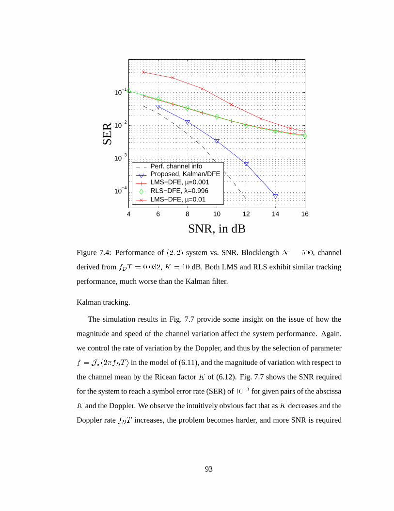
4 6 8 10 12 14 16
10−4
10−3
10−2
10−1
Perf. channel info Proposed, Kalman/DFE LMS−DFE, µ=0.001 RLS−DFE, λ=0.996LMS−DFE, µ=0.01
SNR, in dB
SER
Figure 7.4: Performance of (2; 2) system vs. SNR. Blocklength N = 500, channel
derived from fDT = 0:032, K = 10 dB. Both LMS and RLS exhibit similar tracking
performance, much worse than the Kalman filter.
Kalman tracking.
The simulation results in Fig. 7.7 provide some insight on the issue of how the
magnitude and speed of the channel variation affect the system performance. Again,
we control the rate of variation by the Doppler, and thus by the selection of parameter
f = Jo (2�fDT ) in the model of (6.11), and the magnitude of variation with respect to
the channel mean by the Ricean factor K of (6.12). Fig. 7.7 shows the SNR required
for the system to reach a symbol error rate (SER) of 10�3 for given pairs of the abscissa
K and the Doppler. We observe the intuitively obvious fact that asK decreases and the
Doppler rate fDT increases, the problem becomes harder, and more SNR is required
93
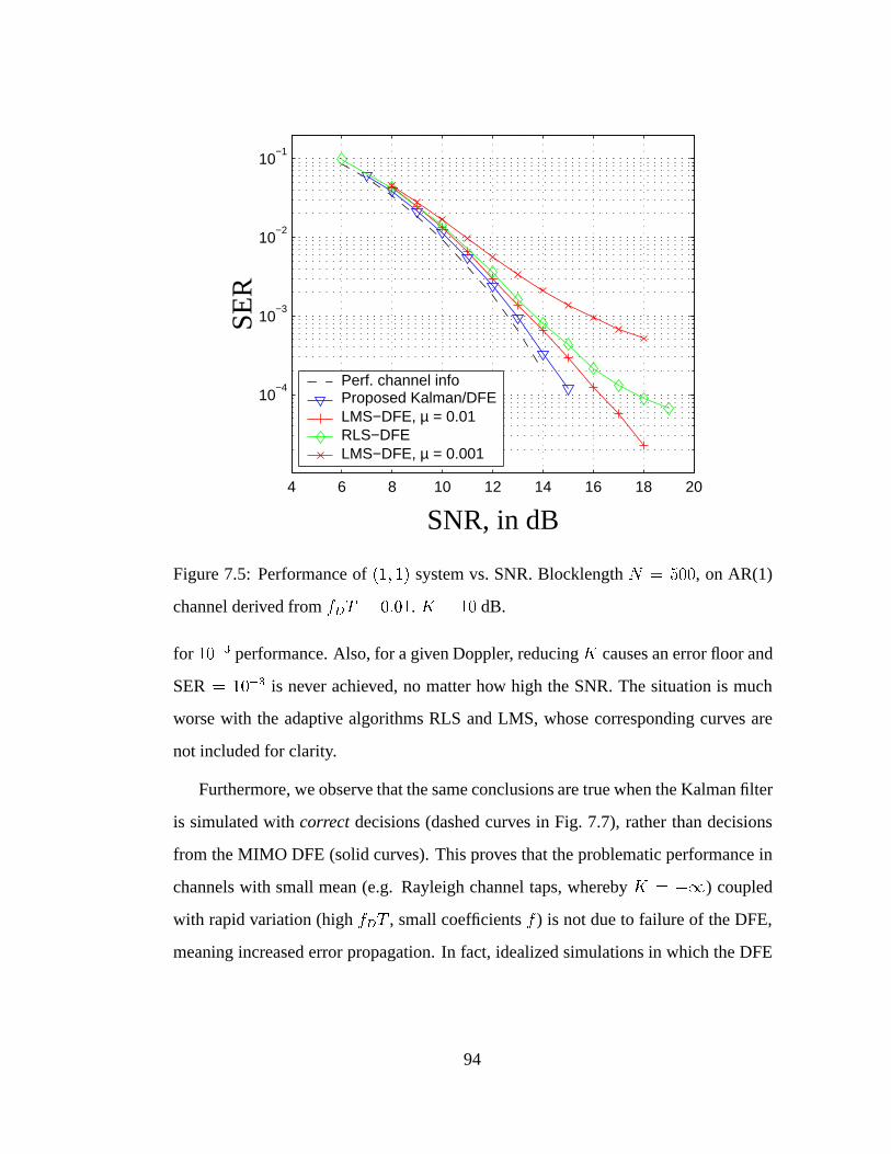
4 6 8 10 12 14 16 18 20
10−4
10−3
10−2
10−1
Perf. channel info Proposed Kalman/DFE LMS−DFE, µ = 0.01 RLS−DFE LMS−DFE, µ = 0.001
SNR, in dB
SER
Figure 7.5: Performance of (1; 1) system vs. SNR. Blocklength N = 500, on AR(1)
channel derived from fDT = 0:01. K = 10 dB.
for 10�3 performance. Also, for a given Doppler, reducing K causes an error floor and
SER = 10�3 is never achieved, no matter how high the SNR. The situation is much
worse with the adaptive algorithms RLS and LMS, whose corresponding curves are
not included for clarity.
Furthermore, we observe that the same conclusions are true when the Kalman filter
is simulated with correct decisions (dashed curves in Fig. 7.7), rather than decisions
from the MIMO DFE (solid curves). This proves that the problematic performance in
channels with small mean (e.g. Rayleigh channel taps, whereby K = �1) coupled
with rapid variation (high fDT , small coefficients f ) is not due to failure of the DFE,
meaning increased error propagation. In fact, idealized simulations in which the DFE
94
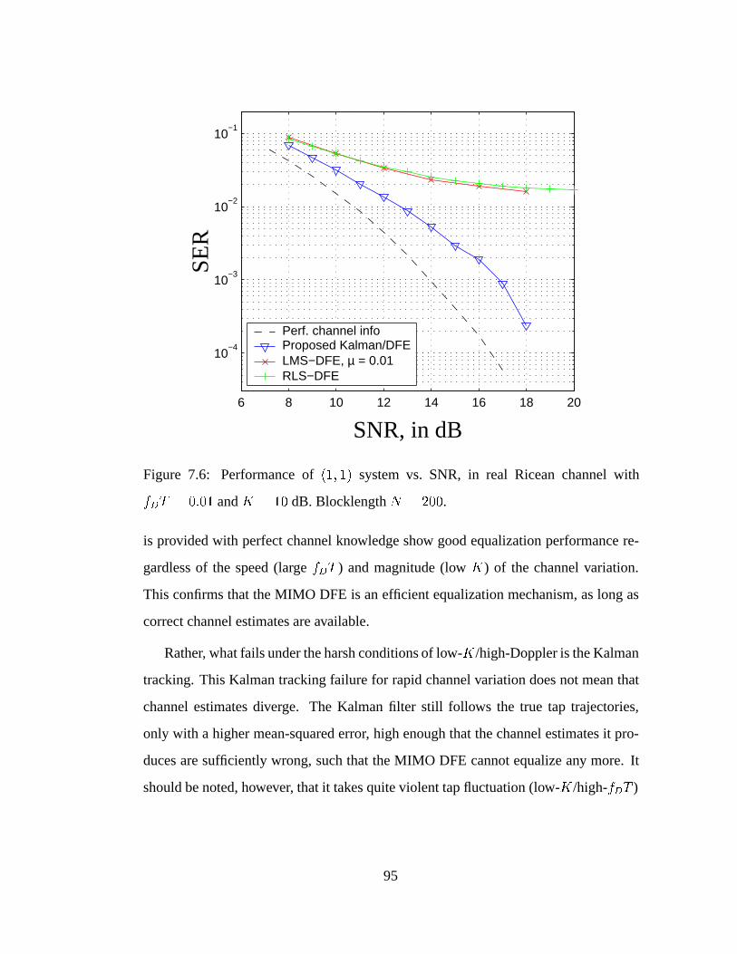
6 8 10 12 14 16 18 20
10−4
10−3
10−2
10−1
Perf. channel info Proposed Kalman/DFELMS−DFE, µ = 0.01RLS−DFE
SNR, in dB
SER
Figure 7.6: Performance of (1; 1) system vs. SNR, in real Ricean channel with
fDT = 0:01 and K = 10 dB. Blocklength N = 200.
is provided with perfect channel knowledge show good equalization performance re-
gardless of the speed (large fDT ) and magnitude (low K) of the channel variation.
This confirms that the MIMO DFE is an efficient equalization mechanism, as long as
correct channel estimates are available.
Rather, what fails under the harsh conditions of low-K/high-Doppler is the Kalman
tracking. This Kalman tracking failure for rapid channel variation does not mean that
channel estimates diverge. The Kalman filter still follows the true tap trajectories,
only with a higher mean-squared error, high enough that the channel estimates it pro-
duces are sufficiently wrong, such that the MIMO DFE cannot equalize any more. It
should be noted, however, that it takes quite violent tap fluctuation (low-K/high-fDT )
95

−6 −4 −2 0 2 4 6 8 10 12 148
10
12
14
16
18
20
22
24
26 GM, fD
T=0.004 GM, f
DT=0.01
GM, fD
T=0.01, Corr. Data GM, f
DT=0.032
GM, fD
T=0.032, Corr. Data
Ricean factor K, in dB
SNR
@10�3
Figure 7.7: SNR required for the (2; 2) system to reach SER = 10�3 for different
channel conditions, i.e. Ricean factor K and Doppler rate. The channel is time-varying
according to the Gauss-Markov (GM) model of (6.11).
to cause the Kalman filter to ineffectively track the taps, while the baseline LMS/RLS
adaptive algorithms exhibit high error floor for much milder channel conditions, and
never outperform the Kalman filter tracking. An additional observation for perspective
is that in the limit of very low K and very high fDT , the channel tap values become
effectively i.i.d., which makes any attempts for channel estimation futile by definition.
7.4 Coding
When the nT transmitter antennas belong to individual, uncoordinated, yet assumed
synchronous users, each of them uses a separate trellis code. Hence, the Kalman track-
96
ing ideas of section 7.1 can be used in a variety of ways, depending on available com-
plexity and desired performance at the receiver. The simplest solution is to do hard trel-
lis decoding for each individual user, using the decisions x(i), i = 1; : : : ; nT produced
by the MIMO DFE. A better approach is to use the soft values ~x(i), i = 1; : : : ; nT
before the slicers in Fig. 7.2 as input to nT independent soft trellis decoders, while of
course continuing to provide the hard decisions x to the feedback section of the DFE
and the Kalman estimator.
Both the above methods however would suffer from error propagation, because
the DFE produces errors in bursts that can defeat the error correcting capabilities of
the individual trellis codes. If the system can tolerate the added latency, one way to
overcome the bursty errors from the DFE is to introduce interleaving of the outputs
of each encoder at the transmitters, and the corresponding deinterleaving operations
on each of the nT streams of soft values prior to the nT decoders at the receiver [52].
A good way to get around this problem without added latency, but with increased
receiver complexity is per-survivor processing (PSP, see [53]), whereby there is one
combination of Kalman filter and MIMO DFE for every combination of survivor paths
between the nT independent trellis decoders. Specifically, if we keep s survivor paths
for every trellis decoder, the number of necessary Kalman/DFE combinations is snT ,
and each of those functions in the way described in section 7.1. The simple solution
with a single Kalman/DFE followed by nT soft trellis decoders mentioned above is a
special case of this last arrangement, with s = 1 survivor path kept per user.
In the case of a single user with nT transmitter and nR = nT receiver antennas
for increased data rate, the correct choice of a coding scheme to fit with the channel
tracking and equalization mechanism discussed in section 7.1 is not obvious. If the
channel were to remain constant for the whole block, and if we could assume perfect
cancellation of ISI and CCI, then the effective vector channel x! ~x could be thought
97
of as nT parallel channels, each with different SNR. Thus, a 1-dimensional trellis
code, coding across transmitter antennas would encounter a periodically time-varying
channel, as noticed for the layered interference cancellation scheme in [48]. Good
trellis codes for periodic channels have been designed in [54] and [55]. However, this
is not the case, since the MIMO channel is neither constant nor perfectly known, and
ISI and CCI cannot be perfectly cancelled. The finite MIMO DFE of section 7.1.2
precludes this by definition. Hence, a periodic code optimized for PECL and PPD (see
[54]) is a suboptimal choice, as confirmed from the coded simulation results marked
with “2” in Fig. 7.8. Such a code might provide better performance if the MIMO DFE
is designed for successive interference cancellation, as described in [44].
To take into account the time variation of the effective channel x ! ~x with a 1-
D code, we chose to optimize this code for diversity. Namely, for the given 4-PSK
modulation and 8 code states, we performed an exhaustive search over all rate-1/2
codes aimed at maximizing the effective code length (ECL, often referred to as the
minimum time-diversity of the code) and the product distance (PD). The best such
code is described by the polynomials g1(D) = 1 + D + D2, g2(D) = 1 + D
2 + D3
and has ECL = 4 and PD = 64 for a Gray-labeled 4-PSK constellation with unit
power. The curve marked with “3” in Fig. 7.8 shows its BER performance with an
8-state Viterbi decoder of traceback depth 14 (the same as for the periodic 1-D code
optimized for PECL and PPD above), fed by the soft equalized values prior to the DFE
slicers.
Clearly, both 1-D trellis codes provide a big coding gain with respect to the raw
error rate at the slicers, although many important details have been ignored at decod-
ing, such as the time-correlation of the noise after the matrix feedforward filter. The
diversity code performs better than the code optimized for periodic channels.
As shown in Fig. 7.8 it is possible to do better than both the 1-D trellis codes
98
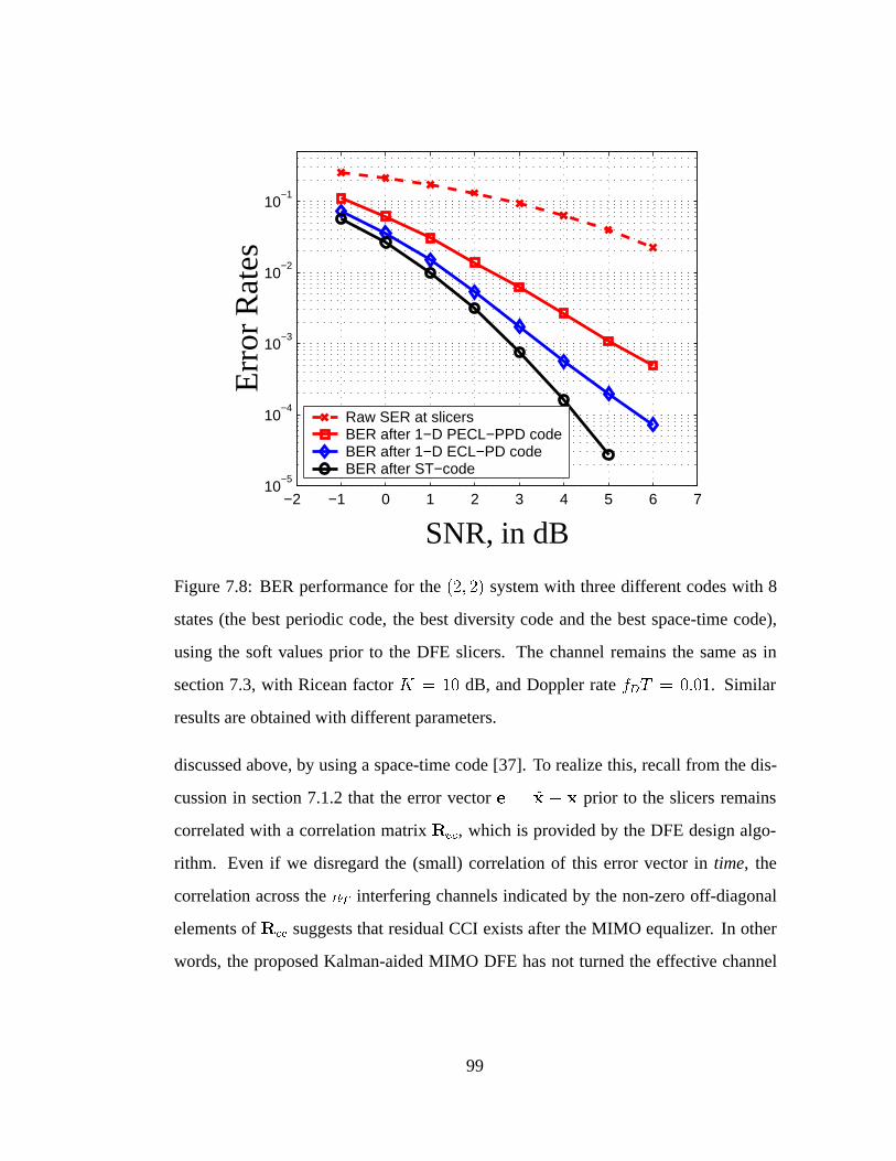
−2 −1 0 1 2 3 4 5 6 710
−5
10−4
10−3
10−2
10−1
Raw SER at slicers BER after 1−D PECL−PPD codeBER after 1−D ECL−PD code BER after ST−code
SNR, in dB
Err
orR
ates
Figure 7.8: BER performance for the (2; 2) system with three different codes with 8
states (the best periodic code, the best diversity code and the best space-time code),
using the soft values prior to the DFE slicers. The channel remains the same as in
section 7.3, with Ricean factor K = 10 dB, and Doppler rate fDT = 0:01. Similar
results are obtained with different parameters.
discussed above, by using a space-time code [37]. To realize this, recall from the dis-
cussion in section 7.1.2 that the error vector e = ~x � x prior to the slicers remains
correlated with a correlation matrix Ree, which is provided by the DFE design algo-
rithm. Even if we disregard the (small) correlation of this error vector in time, the
correlation across the nT interfering channels indicated by the non-zero off-diagonal
elements of Ree suggests that residual CCI exists after the MIMO equalizer. In other
words, the proposed Kalman-aided MIMO DFE has not turned the effective channel
99
x! ~x into nT non-interfering parallel channels, in which case the use of an appropri-
ate 1-D trellis code would be a good choice.
Instead, the vector channel x ! ~x has been turned into a “flat” MIMO channel,
having CCI but mostly devoid of ISI and cross-ISI. Thus, the 8-state space-time code
designed in [37] (see Fig. 5(a) there) is the best coding choice, as shown by the sim-
ulation in Fig. 7.8. For comparison with equal complexity with the 1-D codes above,
we kept the traceback depth of the vector Viterbi decoder to 7, since in this case every
trellis step corresponds to two steps of each 1-D code.
A final note concerns the decoding metric for the Viterbi decoder in both situations
(1-D codes and space-time code). Since we are aware of the correlation across trans-
mitted symbols, the correct metric for assumed transmitted vector xk and “received”
equalized vector ~x is not k~x� xkk2. Rather, it is expressed by:
M(k) = (~x� xk)�R�1ee (~x� xk); (7.13)
where Ree is the error vector correlation matrix, which is provided as a by-product of
the MIMO DFE design. The computation of the metric of (7.13) was implemented
for both the space-time trellis decoder and the two 1-D trellis decoders. In the latter
case one just needs to combine two trellis steps in one, effectively producing a rate-
2=4 trellis code, transmitting two 4-PSK symbols at a time, very similar to the space-
time code. Since essentially the same decoding is implemented, it is clear that the
improved BER performance of the space-time code has to do solely with its ability to
combat residual interference more effectively than the 1-D codes, which are encoding
across transmitter antennas. This is not surprising, because the 1-D trellis codes were
designed to provide diversity (periodic or not, respectively) and were not intended to
overcome the coupling of interfering streams of data like the space-time code.
100
7.5 Conclusions
This second part of the dissertation (Chapters 6 and 7) discussed a receiver structure
to track and equalize a MIMO frequency selective fading channel. A Kalman filter
was used for tracking the channel, and an MMSE DFE, optimized for decision delay
� � 0 to equalize the channel and suppress CCI. The time gap between channel
estimates produced by the Kalman filter and those needed for the DFE adaptation was
bridged by using a simple prediction module. This algorithm, in exchange for larger
complexity when compared to simple LMS/RLS updates of the DFE, offers improved
performance and good tracking behavior for long unsupervised blocks, close to the
performance of the idealistic case where perfect channel information is available at the
receiver. Additionally, appropriate trellis coding options compatible with this method
for tracking and equalization were discussed.
101
CHAPTER 8
Conclusions and Future Work
This dissertation presented algorithms to estimate fading in a wireless channel, while
simultaneously decoding a turbo-code in flat fading (first part) or equalizing a MIMO
frequency-selective channel (second part).
Turbo-decoding in flat and frequency selective fading, without assuming prior
knowledge of the channel, has recently attracted the attention of researchers as wireless
applications become more dominant and processing capabilities of receivers increase.
Some examples are the work in [56] proposing adaptive SISO decoders, differential
detection in [57], which deteriorates at high Doppler, as well as the research in [21]
and [20], which is similar to the iterative Wiener filtering approach in Chapter 5 of this
dissertation.
Areas for future research include performance in conjunction with complexity, tak-
ing into account implementation issues such as fixed point arithmetic in digital signal
processors and timing jitter. Further research should also explore accurate capacity
computation for the fading models discussed in Chapter 3, with nonzero autocorrela-
tion for infinite lag. Research attempts in this domain include the capacity of finite-
state Markov channels in [29], which is computationally cumbersome and still only an
approximation, the bounds derived here in Chapter 4, as well as work in [27] for other
correlation models, and [58] in a more general setting. Computing channel capacity
corresponding to different algorithms of channel acquisition will provide an absolute
measure for performance evaluation in any Doppler rate and SNR operation point.
102
For the problem of achieving reliable communication in a MIMO time-varying
frequency-selective channel, treated in the second part of this dissertation, the research
effort has been increasing in the past few years, as the market demands ever higher
data rates in a difficult wireless environment. This dissertation presents an algorithm
for channel tracking and equalization based on Kalman filtering and a MIMO MMSE
DFE of finite length, but a number of issues remain open. For instance, initial training
of the MIMO equalizer (before going into tracking mode) discussed in [59], is a sig-
nificant area for further research. But more importantly, code design must be done for
MIMO systems such that the code is compatible with the signal processing strategy
for interference avoidance and cancellation, see [60] and [61, 62] and [48], seeking a
code that will help approach the vast capacities promised in [2]. Significant research
contributions in this domain are the space-time codes of [37], as well as the work in
[63] and the combination of space and time diversity in [64], but much remains to be
done, particularly if the great error-correcting potential of turbo-codes is also to be
exploited in the MIMO environment.
On a different note, as signaling rates inevitably increase, the inter-symbol interfer-
ence in the channel becomes more severe, and then equalization is no longer a practi-
cal solution, because of the overhead associated with training long complex equalizers
(e.g. a MIMO DFE). In this case, the signaling paradigm of MIMO multicarrier mod-
ulation as in [65] is probably more appropriate, since it provides more natural coding
options that can approach capacity. Besides, the channel then becomes flat (viewed in
the frequency domain), which facilitates both estimation and equalization, apart from
the positive impact on the design of an appropriate channel coding scheme.
103
APPENDIX A
Estimation from Pilot Symbols
Let a sequence fxtg of multiplexed coded data and known pilot symbols be transmitted
in a flat Rayleigh fading channel. Then, the observed sequence is yt = at � xt + nt,
where xt is a pilot (a known symbol) if t mod (D + Z) < Z, and an unknown
coded symbol if t mod (D+Z) � Z. This arrangement assumes that the transmitter
sends frames of D consecutive coded symbols between frames of Z consecutive pilot
symbols, and in this dissertation all symbols come from a PSK constellation and thus
have unit energy.
The purpose of an optimum (in the minimum mean-square sense) pilot-only fil-
ter (POF) at the receiver is to operate on the observations corresponding to pilots and
render optimum channel estimates ak, k = 0; 1; : : : ; D� 1 for the times t correspond-
ing to unknown transmitted data. If the one-sided length of the POF is L0 pilot slots
(therefore a total of 2L0Z pilot symbols), then there are D distinct optimum POFs W ok ,
k = 0; 1; : : : ; D � 1, each operating on L0Z symbols on both sides of the channel es-
timate for time k. In fact, due to symmetry in time, these D POFs (horizontal vectors)
Wok , k = 0; 1; : : : ; D � 1 are mirrored versions of each other for indices k that are
equidistant from 0 and D � 1.
Since only observations coming from pilot symbols are going to be filtered, we can
equally well filter the derotated versions ~y of the pilot symbols, after the effect of the
104
pilot x has been removed, namely:
~y = a+ ~n: (A.1)
Observe that since pilots have unit energy, this derotation does not affect the noise
statistics, so ~n are still i.i.d. complex Gaussian random variables with variance �2 per
dimension.
Collecting all the relevant derotated observations ~y in a column vector ~y of length
2L0Z, the problem is to optimally estimate ak, k = 0; 1; : : : ; D � 1 from ~y = a + ~n.
Fig. A.1 gives an example of a received stream, and the pilot-filtering operation for
D = 5, Z = 3, L0 = 2. Note that in this appendix we ignore the “edge-effects” that
occur when the channel coefficients to be estimated are located close to the edges of a
block of data, where the receiver might not have access to L0 pilot slots on either side
of the desired channel coefficient. In other words, the derivations below require L0
pilot slots (of Z symbols each) on either side of the frame of D coded data symbols,
for which the channel gains ak, k = 0; 1; : : : ; D � 1 are being estimated. The special
cases that occur when fewer than L0 pilot slots exist on one side are straightforward to
obtain.
From linear estimation theory it is well-known that since the complex vectors a,
~n and ~y are zero-mean, the optimum linear estimator of the scalar ak (and also the
optimum estimator when nonlinear estimators are considered, since all variables are
complex Gaussian) is:
Wok = Eak~y
� � [E~y~y�]�1
= Rak;~y �R�1~y ; k = 0; 1; : : : ; D � 1 (A.2)
where Rak;~y is a horizontal vector of length 2L0Z with entries:
Rak ;~y(i) = Jo (2�fDT � index(i; k)) ; (A.3)
105

p p p p p p p p pd d d d d d d d d d d d d d d
0 D-1k
p p p
k = 1: Estimate a1.
~yT
Figure A.1: Collection of the derotated observables corresponding to pilots into the
vector ~y for D = 5, Z = 3, L0 = 2. “p” denotes observation corresponding to a pilot
symbol, while “d” denotes an observation due to a coded data symbol. The optimum
filters W ok , k = 0; 1; : : : ; D � 1, operate on ~y to estimate ak, k = 0; 1; : : : ; D � 1.
where Jo(�) is the zero-order modified Bessel function of the first kind and
index(i; k) =
8<: (L0 � bi=Zc � 1) �D + (L0Z � i) + k; 0 � i < L0Z
(bi=Zc � L0) �D + (i� L0Z) +D � k; L0Z � i < 2L0Z
(A.4)
The covariance matrix of the vector ~y is:
R~y = Ra + 2�2I2L0Z; (A.5)
where the matrix Ra = Eaa� is symmetric but not Toeplitz, since the symbols corre-
sponding to the fading coefficients inside the vector a were not necessarily adjacent in
the initial data stream. The entries of the matrix Ra are:
Ra(i; j) = Jo (2�fDT � [D � jbi=Zc � bj=Zcj+ ji� jj]) ; i; j = 0; : : : ; 2L0Z � 1:
(A.6)
To verify the non-Toeplitz structure of the matrix Ra, observe that:
Ra(0; 2) = Jo (2�fDT � 2) 6= Jo (2�fDT � (D + 2)) = Ra(1; 3): (A.7)
106
From (A.2) and using (A.3)–(A.6) it is straightforward to compute the D distinct
optimum POFs W ok , each of which provides the estimates:
ak = Wok � ~y; k = 0; 1; : : : ; D � 1: (A.8)
The minimum mean-squared error (m.m.s.e.) of the estimation is (see, for instance,
[34]):
Ej~akj2 def= Ejak � akj2 (A.9)
= 1� Rak;~yR�1y R
�ak ;~y
(A.10)
= 1�Wok (Ra + I2L0Z) (W
ok )�; (A.11)
and the average m.m.s.e. due to estimation from pilots can be obtained:
MSE =
D�1Xk=0
Ej~akj2; (A.12)
which is the quantity plotted against SNR in Fig. 3.3.
107
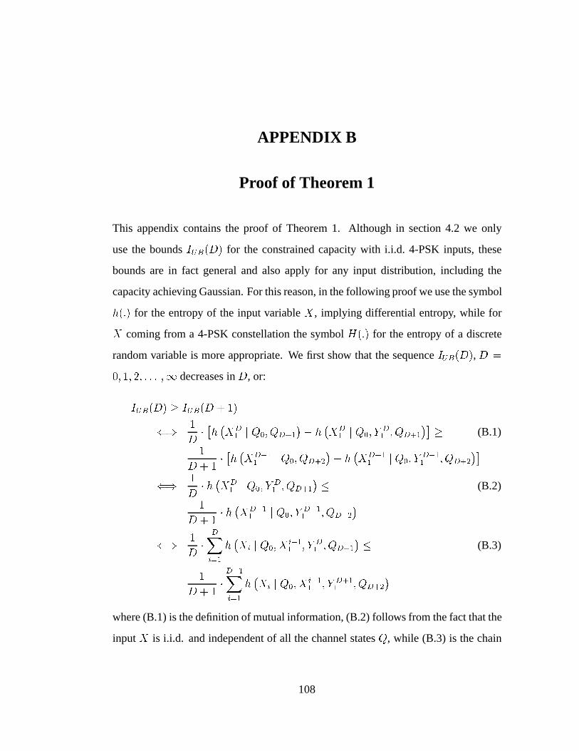
APPENDIX B
Proof of Theorem 1
This appendix contains the proof of Theorem 1. Although in section 4.2 we only
use the bounds IUB(D) for the constrained capacity with i.i.d. 4-PSK inputs, these
bounds are in fact general and also apply for any input distribution, including the
capacity achieving Gaussian. For this reason, in the following proof we use the symbol
h(:) for the entropy of the input variable X , implying differential entropy, while for
X coming from a 4-PSK constellation the symbol H(:) for the entropy of a discrete
random variable is more appropriate. We first show that the sequence IUB(D), D =
0; 1; 2; : : : ;1 decreases in D, or:
IUB(D) � IUB(D + 1)
() 1
D
� �h �XD1 j Q0; QD+1
�� h
�X
D1 j Q0; Y
D1 ; QD+1
�� � (B.1)
1
D + 1� �h �XD+1
1 j Q0; QD+2
�� h
�X
D+11 j Q0; Y
D+11 ; QD+2
��() 1
D
� h �XD1 j Q0; Y
D1 ; QD+1
� � (B.2)
1
D + 1� h �XD+1
1 j Q0; YD+11 ; QD+2
�() 1
D
�DXi=1
h
�Xi j Q0; X
i�11 ; Y
D1 ; QD+1
� � (B.3)
1
D + 1�D+1Xi=1
h
�Xi j Q0; X
i�11 ; Y
D+11 ; QD+2
�where (B.1) is the definition of mutual information, (B.2) follows from the fact that the
input X is i.i.d. and independent of all the channel states Q, while (B.3) is the chain
108
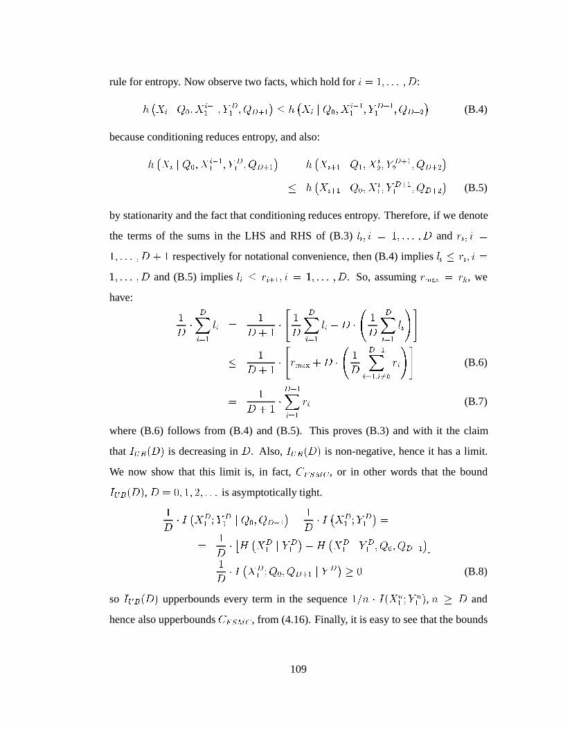
rule for entropy. Now observe two facts, which hold for i = 1; : : : ; D:
h
�Xi j Q0; X
i�11 ; Y
D1 ; QD+1
� � h
�Xi j Q0; X
i�11 ; Y
D+11 ; QD+2
�(B.4)
because conditioning reduces entropy, and also:
h
�Xi j Q0; X
i�11 ; Y
D1 ; QD+1
�= h
�Xi+1 j Q1; X
i2; Y
D+12 ; QD+2
�� h
�Xi+1 j Q0; X
i1; Y
D+11 ; QD+2
�(B.5)
by stationarity and the fact that conditioning reduces entropy. Therefore, if we denote
the terms of the sums in the LHS and RHS of (B.3) li; i = 1; : : : ; D and ri; i =
1; : : : ; D + 1 respectively for notational convenience, then (B.4) implies li � ri; i =
1; : : : ; D and (B.5) implies li � ri+1; i = 1; : : : ; D. So, assuming rmax = rk, we
have:
1
D
�DXi=1
li =1
D + 1�"1
D
DXi=1
li +D �
1
D
DXi=1
li
!#
� 1
D + 1�"rmax +D �
1
D
D+1Xi=1;i6=k
ri
!#(B.6)
=1
D + 1�D+1Xi=1
ri (B.7)
where (B.6) follows from (B.4) and (B.5). This proves (B.3) and with it the claim
that IUB(D) is decreasing in D. Also, IUB(D) is non-negative, hence it has a limit.
We now show that this limit is, in fact, CFSMC , or in other words that the bound
IUB(D), D = 0; 1; 2; : : : is asymptotically tight.
1
D
� I �XD1 ;Y D
1 j Q0; QD+1
�� 1
D
� I �XD1 ;Y D
1
�=
=1
D
� �H �XD1 j Y D
1
��H
�X
D1 j Y D
1 ; Q0; QD+1
��=
1
D
� I �XD1 ;Q0; QD+1 j Y D
1
� � 0 (B.8)
so IUB(D) upperbounds every term in the sequence 1=n � I(Xn1 ;Y
n1 ), n � D and
hence also upperbounds CFSMC , from (4.16). Finally, it is easy to see that the bounds
109
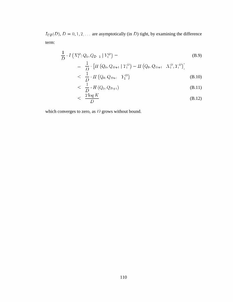
IUB(D), D = 0; 1; 2; : : : are asymptotically (in D) tight, by examining the difference
term:
1
D
� I �XD1 ;Q0; QD+1 j Y D
1
�= (B.9)
=1
D
� �H �Q0; QD+1 j Y D1
��H
�Q0; QD+1 j XD
1 ; YD1
��� 1
D
�H �Q0; QD+1 j Y D1
�(B.10)
� 1
D
�H (Q0; QD+1) (B.11)
� 2 logK
D
(B.12)
which converges to zero, as D grows without bound.
110
REFERENCES
[1] C. Berrou, A. Glavieux, and P. Thitimajshima. Near Shannon limit error-correcting coding and decoding: Turbo-codes (1). In ICC ’93, pages 1064–1070,1993.
[2] G. J. Foschini and M. J. Gans. On limits of wireless communications in a fadingenvironment when using multiple antennas. Wireless Personal Communications,6:311–35, 1998.
[3] S. Benedetto and G. Montorsi. Unveiling turbo codes: Some results on parallelconcatenated coding schemes. IEEE Trans. on Inform. Theory, 42(2):409–428,March 1996.
[4] E. K. Hall and S. G. Wilson. Design and analysis of turbo-codes on Rayleighfading channels. IEEE Journal on Sel. Areas in Comm., 16(2):160–174, Feb.1998.
[5] C. Fragouli and R. Wesel. Symbol-interleaved parallel concatenated trellis codedmodulation. 1999 IEEE Communication Theory Miniconference in conjunctionwith ICC 99, Vancouver, BC, Canada, 6-10 June 1999.
[6] C. Fragouli. Turbo-Code Design for High Spectral Efficiency. PhD thesis,UCLA, 2000.
[7] S. Benedetto , D. Divsalar, G. Montorsi, and F. Pollara. Parallel concatenatedtrellis coded modulation. IEEE International Conference on Communications,ICC 1996, Dallas, TX, 2, June 1996.
[8] S. Benedetto , D. Divsalar, G. Montorsi, and F. Pollara. A soft-input soft-outputAPP module for the iterative decoding of concatenated codes. IEEE Communi-cations Letters, 1(1):22–4, Jan. 1997.
[9] S. Benedetto , D. Divsalar, G. Montorsi, and F. Pollara. Soft-input soft-outputmodules for the construction and distributed iterative decoding of code networks.Europ. Trans. on Telecom., 9(2):155–172, March-April 1998.
[10] C. Fragouli and R. Wesel. Turbo encoder design for symbol-interleaved paral-lel concatenated trellis coded modulation. to appear in IEEE Transactions onCommunications, 2000.
[11] P. Robertson and T. Worz. Bandwidth-efficient turbo trellis-coded modulationusing punctured component codes. IEEE Journal on Sel. Areas in Comm.,16(2):206–18, Feb. 1998.
111
[12] L. R. Bahl, J. Cocke, F. Jelinek, and J. Raviv. Optimal decoding of linear codesfor minimizing symbol error rate. IEEE Trans. on Inform. Theory, 20(2):284–287, March 1974.
[13] L. E. Baum, T. Petrie, G. Soules, and N. Weiss. A maximization technique occur-ing in the statistical analysis of probabilistic functions of Markov chains. Ann.Math. Stat, 41:164–171, 1970.
[14] L. R. Rabiner and B.-H. Juang. Fundamentals of Speech Recognition. PrenticeHall, Englewood Cliffs, N.J., 1993.
[15] R. H. Clarke. A statistical theory of mobile radio reception. Bell Syst. Tech. J.,pages 957–1000, July 1968.
[16] W. C. Y. Lee. Mobile Communications Engineering. McGraw Hill, NY, 1982.
[17] W. C. Jakes, Jr. Microwave Mobile Communications. John Wiley & Sons, NY,1974.
[18] H. S. Wang and N. Moayeri. Finite-state Markov channel: A useful model for ra-dio communication channels. IEEE Trans. on Veh. Tech., 44(1):163–171, Febru-ary 1995.
[19] H. S. Wang and P. C. Chang. On verifying the first-order Markovian assumptionfor a Rayleigh fading channel model. IEEE Trans. on Veh. Tech., 45(2):353–357,May 1996.
[20] H. J. Su and E. Geraniotis. Improved performance of a PSAM system with itera-tive filtering and decoding. Thirty-Sixth Annual Allerton Conference on Commu-nication, Control and Computing, pages 156–166, Sept. 1998.
[21] M. C. Valenti and B. D. Woerner. Refined channel estimation for coherent detec-tion of turbo-codes over flat fading channels. Electronics Letters, 34(17):1648–9,Aug. 1998.
[22] A. Papoulis. Probability, Random Variables and Stochastic Processes, 3rd Ed.McGraw-Hill, 1991.
[23] J. K. Cavers. An analysis of pilot symbol assisted modulation for Rayleigh fadingchannels. IEEE Trans. on Veh. Tech., 40(4):686–693, Nov. 1991.
[24] A. G. Dabak, S. Hosur, and T. Schmidl. Iterative channel estimation for wide-band CDMA systems. Thirty-Sixth Annual Allerton Conference on Communica-tion, Control and Computing, pages 441–9, Sep. 1998.
112
[25] R. G. Gallager. Information Theory and Reliable Communication. New York:Wiley, 1968.
[26] L. H. Ozarow, Shlomo Shamai, and A. D. Wyner. Information theoretic consid-erations for cellular mobile radio. IEEE Trans. on Veh. Tech., 43(2):369–378,May 1994.
[27] G. Kaplan and Shlomo Shamai. Achievable performance over the correlatedRician channel. IEEE Trans. on Comm., 42(11):2967–2978, Nov. 1994.
[28] M. Mushkin and I. Bar-David. Capacity and coding for the Gilbert-Elliott chan-nels. IEEE Trans. on Inform. Theory, 35(6):1277–1290, Nov. 1989.
[29] A. J. Goldsmith and P. P. Varaiya. Capacity, mutual information, and coding forfinite-state Markov channels. IEEE Trans. on Inform. Theory, 42(3):868–886,May 1996.
[30] J. G. Proakis. Digital Communications, Third Edition. McGraw-Hill, 1995.
[31] R. Price and P. E. Green, Jr. A communication technique for multipath channels.Proceed. IRE, 46:555–70, March 1958.
[32] P. A. Bello. Performance of some RAKE modems over the nondisturbed wideband HF channel. Proc. of 1989 IEEE Military Commun. Conf. (MIL-COM),pages 39.3.1–39.3.4, September 1989.
[33] G. D. Forney, Jr. and G. Ungerboeck. Modulation and coding for linear Gaussianchannels. IEEE Trans. on Inform. Theory, 44(6):2384–2415, Oct. 1998.
[34] T. Kailath, A. H. Sayed, and B. Hassibi. Linear Estimation. Prentice Hall, NJ,2000.
[35] A. Duel-Hallen. A family of multiuser decision-feedback detectors for asyn-chronous code-division, multiple-access channels. IEEE Trans. on Comm., pages421–34, Feb/Mar/April 1995.
[36] M. Honig, U. Madhow, and S. Verdu. Blind adaptive multiuser detection. IEEETrans. on Inform. Theory, 41(4):944–60, July 1995.
[37] V. Tarokh, N. Seshadri, and A. R. Calderbank. Space-time codes for highdata rate wireless communication: Performance criterion and code construction.IEEE Trans. on Inform. Theory, 44(2):744–65, March 1998.
[38] S. U. H. Qureshi. Adaptive equalization. Proc. of the IEEE, 73(9):1349–87,Sept. 1985.
113
[39] D. P. Taylor, G. M. Vitetta, B. D. Hart, and A. Mammela. Wireless channelequalisation. Europ. Trans. on Telecom., 9(2):117–43, March-April 1998.
[40] C. Komninakis, C. Fragouli, A.H. Sayed, and R.D. Wesel. Channel estimationand equalization in fading. Proc. of 33rd Asilomar Conference on Signals, Sys-tems and Computers, pages 1159–1163, Oct. 1999.
[41] G. Paparisto and K. M. Chugg. PSP array processing for multipath fading chan-nels. IEEE Trans. on Comm., 47(4):504–7, April 1999.
[42] S. N. Diggavi, B. C. Ng, and A. Paulraj. An interference suppression schemewith joint channel-data estimation. IEEE Journal on Sel. Areas in Comm.,17(11):1924–39, Nov. 1999.
[43] Y. Li and K. J. R. Liu. Adaptive blind source separation and equalizationfor multiple-input/multiple-output systems. IEEE Trans. on Inform. Theory,44(7):2864–76, Nov. 1998.
[44] N. Al-Dhahir and A. H. Sayed. The finite-length multi-input multi-outputMMSE-DFE. IEEE Trans. on Signal Processing, 48(10):2921–36, Oct. 2000.(see also Proc. of 33-rd Asilomar Conference on Signals, Systems and Comput-ers, pp. 207–209, Oct. 1999).
[45] R. A. Iltis. Joint estimation of PN code delay and multipath using extendedKalman filter. IEEE Trans. on Comm., 38(10):1677–1685, Oct. 1990.
[46] S. Haykin, A. H. Sayed, J. R. Zeidler, P. Yee, and P. C. Wei. Adaptive tracking oflinear time-variant systems by extended RLS algorithms. IEEE Trans. on SignalProcessing, 45(5):1118–1128, May 1997.
[47] P. A. Bello. Characterization of randomly time-variant linear channels. Trans.on Communication Systems, CS(11):360–393, Dec. 1963.
[48] G. J. Foschini. Layered space-time architecture for wireless communication ina fading environment when using multi-element antennas. Bell Labs TechnicalJournal, pages 41–59, Autumn 1996.
[49] M. K. Tsatsanis, G. B. Giannakis, and G. Zhou. Estimation and equalization offading channels with random coefficients. Signal Processing, 53(2-3):211–229,Sept. 1996.
[50] A. H. Sayed and T. Kailath. Extended Chandrasekhar recursions. IEEE Trans.on Aut. Control, 39(3):619–623, Mar. 1994.
[51] S. Haykin. Adaptive Filter Theory, 3rd edition. Prentice Hall, NJ, 1996.
114
[52] M. Vedat Eyuboglu. Detection of coded modulation signals on linear, severelydistorted channels using Decision-Feedback noise prediction with interleaving.IEEE Trans. on Comm., 36(8):401–9, April 1988.
[53] R. Raheli, A. Polydoros, and C.-K. Tzou. Per-survivor processing: a generalapproach to MLSE in uncertain environments. IEEE Trans. on Comm., 43(2-4,pt. 1):354–64, Feb.-April 1995.
[54] R. D. Wesel and J. M. Cioffi. Trellis code design for periodic interleavers. Com-munications Letters, 3(4):103–5, April 1999.
[55] R. D. Wesel, X. Liu, and W. Shi. Trellis codes for periodic erasures. IEEE Trans.on Comm., 48(6):938–47, June 2000.
[56] A. Anastasopoulos and K. M. Chugg. Adaptive soft-input soft-output algorithmsfor iterative detection with parametric uncertainty. IEEE Trans. on Comm.,48(10):1638–49, Oct. 2000.
[57] I. D. Marsland and P. T. Mathiopoulos. Multiple differential detection of paral-lel concatenated convolutional (turbo) codes in correlated fast Rayleigh fading.IEEE Journal on Sel. Areas in Comm., 16(2):265–75, Feb. 1998.
[58] M. Medard. The effect upon channel capacity in wireless communications ofperfect and imperfect knowledge of the channel. IEEE Trans. on Inform. Theory,46(3):933–46, May 2000.
[59] T. L. Marzetta. BLAST training: Estimating channel characteristics for highcapacity space-time wireless. in Proc. of Thiry-Seventh Annual Allerton Confer-ence on Communication, Control, and Computing, Monticello, IL, USA, 23-25Sept. 1998., pages 431–40, 1998.
[60] V. Tarokh, A. Naguib, N. Seshadri, and A. R. Calderbank. Combined array pro-cessing and space-time coding. IEEE Trans. on Inform. Theory, 45(4):1121–8,May 1999.
[61] G. J. Foschini, G. D. Golden, R. A. Valenzuela, and P. W. Wolniansky. Simplifiedprocessing for high spectral efficiency wireless communication employing multi-element arrays. IEEE Journal on Sel. Areas in Comm., 17(11):1841–52, Nov.1999.
[62] P. W. Wolniansky, G. J. Foschini, G. D. Golden, and R. A. Valenzuela. V-BLAST:an architecture for realizing very high data rates over the rich-scattering wirelesschannel. in Proc. of 1998 URSI International Symposium on Signals, Systems,and Electronics, Pisa, Italy, 29 Sept.-2 Oct. 1998, pages 295–300, 1998.
115
[63] S. L. Ariyavisitakul. Turbo space-time processing to improve wireless channelcapacity. In proceedings of ICC 2000, N. Orleans, LA, pages 1238–42, 18-22June 2000.
[64] A. R. Calderbank, G. Pottie, and N. Seshadri. Cochannel interference suppres-sion through time/space diversity. IEEE Trans. on Inform. Theory, 46(3):922–32,May 2000.
[65] G. G. Raleigh and J. M. Cioffi. Spatio-temporal coding for wireless communica-tion. IEEE Trans. on Comm., 46(3):357–66, March 1998.
116


