Trees of genes within species
Joe Felsenstein
University of Washington, Seattle
Trees of genes within species – p.1/77
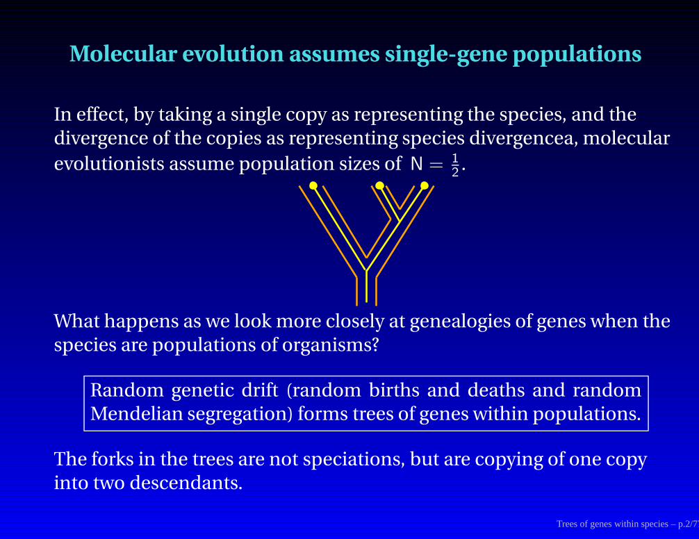
Molecular evolution assumes single-gene populations
In effect, by taking a single copy as representing the species, and the
divergence of the copies as representing species divergencea, molecular
evolutionists assume population sizes of N = 12
.
What happens as we look more closely at genealogies of genes when the
species are populations of organisms?
Random genetic drift (random births and deaths and randomMendelian segregation) forms trees of genes within populations.
The forks in the trees are not speciations, but are copying of one copy
into two descendants.
Trees of genes within species – p.2/77

The Wright-Fisher model
This is the canonical model of genetic drift in populations. It was
invented in 1932 and 1930 by Sewall Wright and R. A. Fisher.
In this model the next generation is produced by doing this:
Choose two individuals with replacement (including the possibilitythat they are the same individual) to be parents,
Each produces one gamete, these become a diploid individual,
Repeat these steps until N diploid individuals have been produced.
The effect of this is to have each locus in an individual in the nextgeneration consist of two genes sampled from the parents’ generation at
random, with replacement.
Trees of genes within species – p.3/77
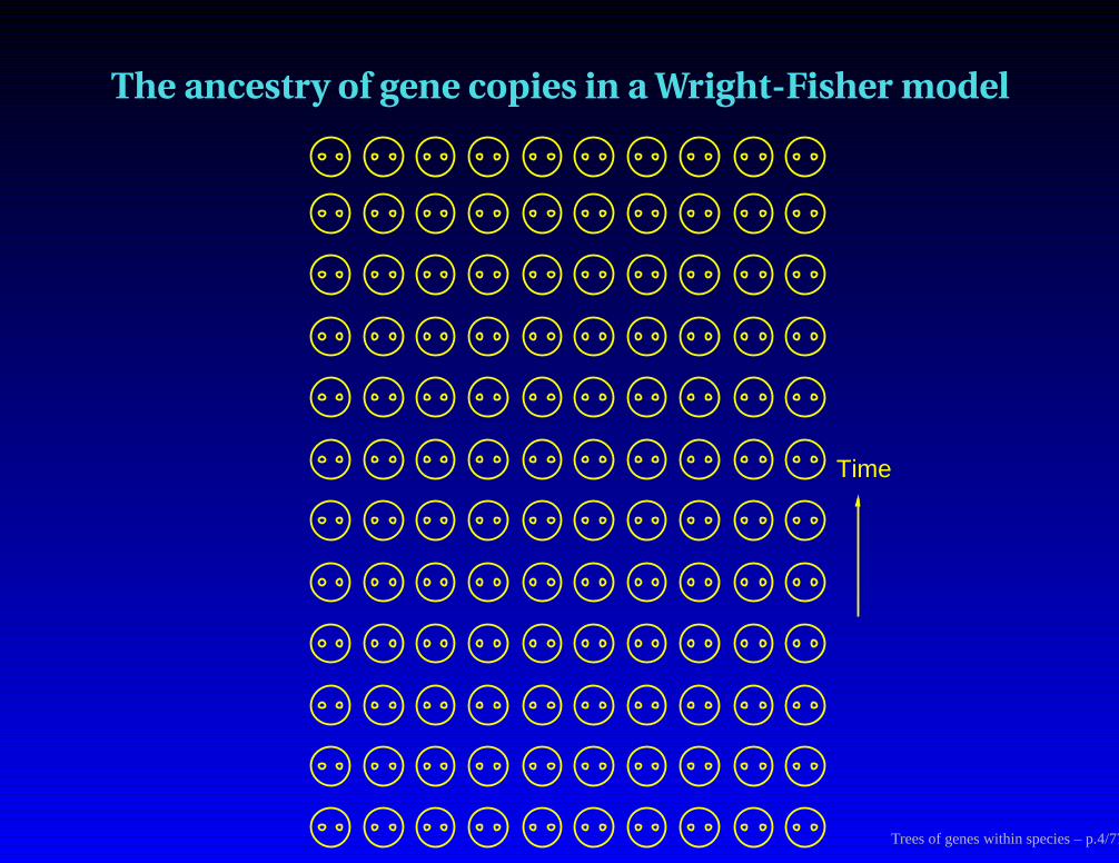
The ancestry of gene copies in a Wright-Fisher model
Time
Trees of genes within species – p.4/77
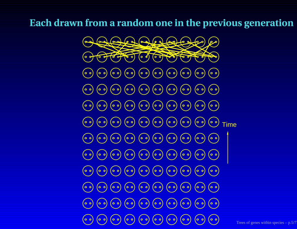
Each drawn from a random one in the previous generation
Time
Trees of genes within species – p.5/77
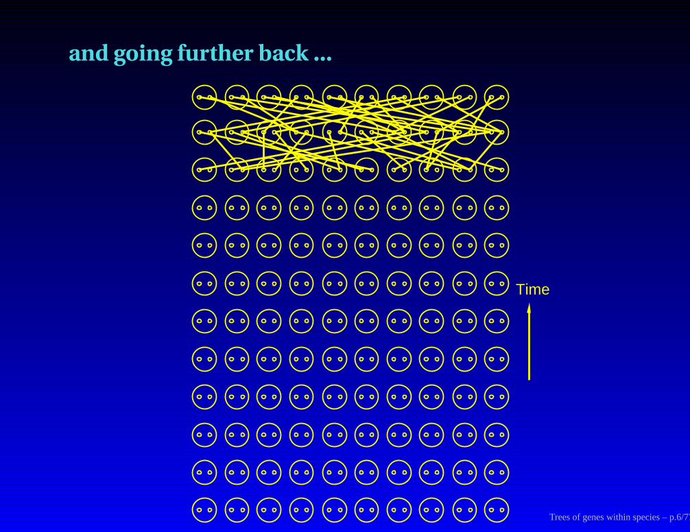
and going further back ...
Time
Trees of genes within species – p.6/77
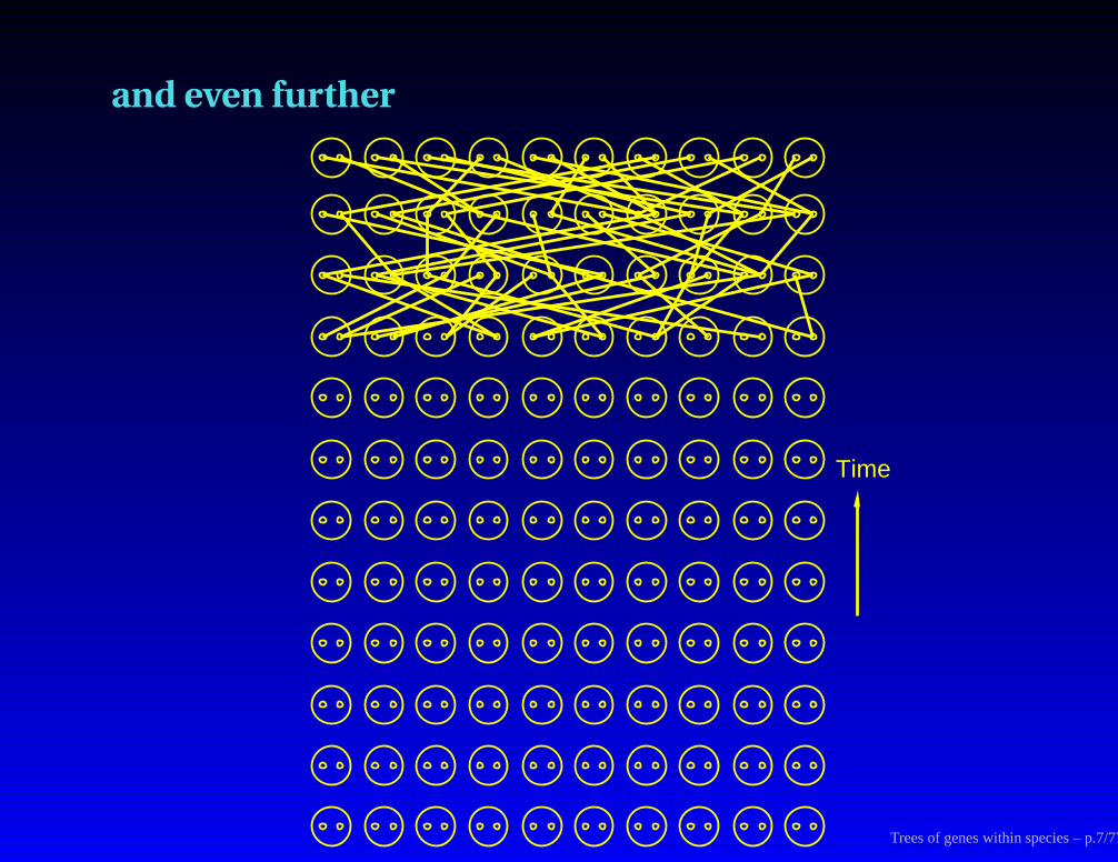
and even further
Time
Trees of genes within species – p.7/77
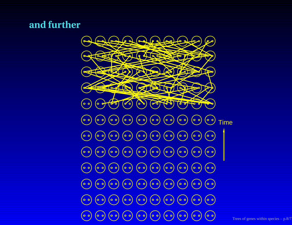
and further
Time
Trees of genes within species – p.8/77
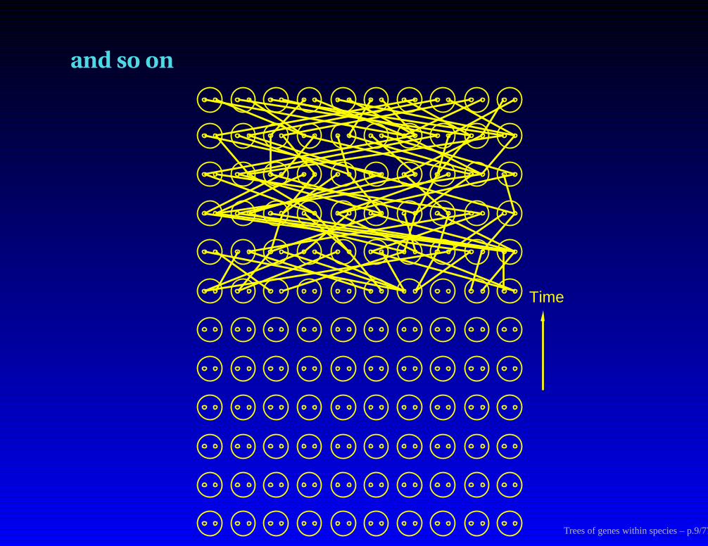
and so on
Time
Trees of genes within species – p.9/77
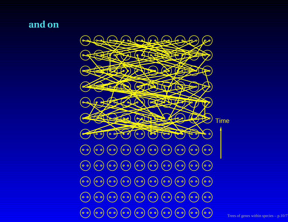
and on
Time
Trees of genes within species – p.10/77
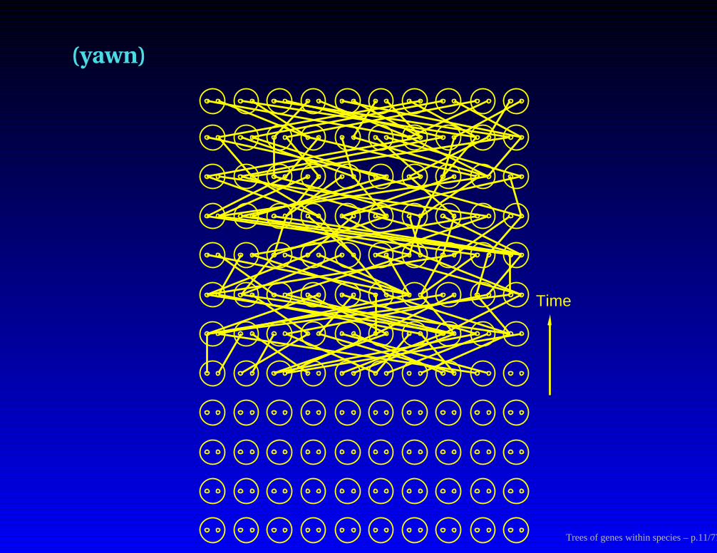
(yawn)
Time
Trees of genes within species – p.11/77
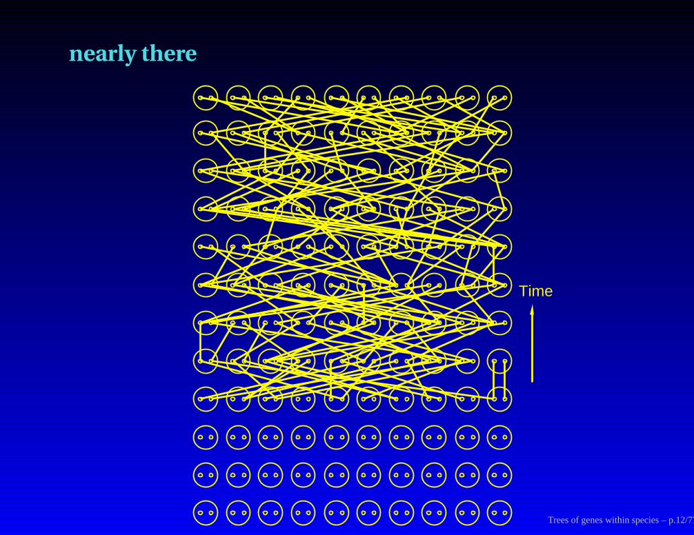
nearly there
Time
Trees of genes within species – p.12/77
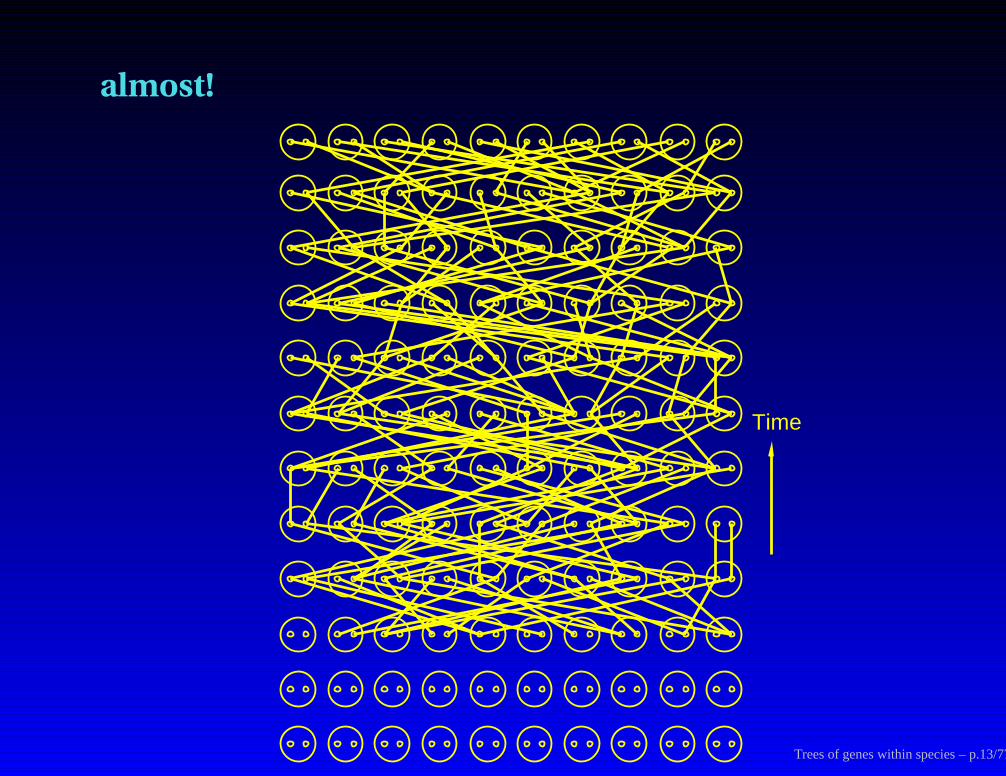
almost!
Time
Trees of genes within species – p.13/77
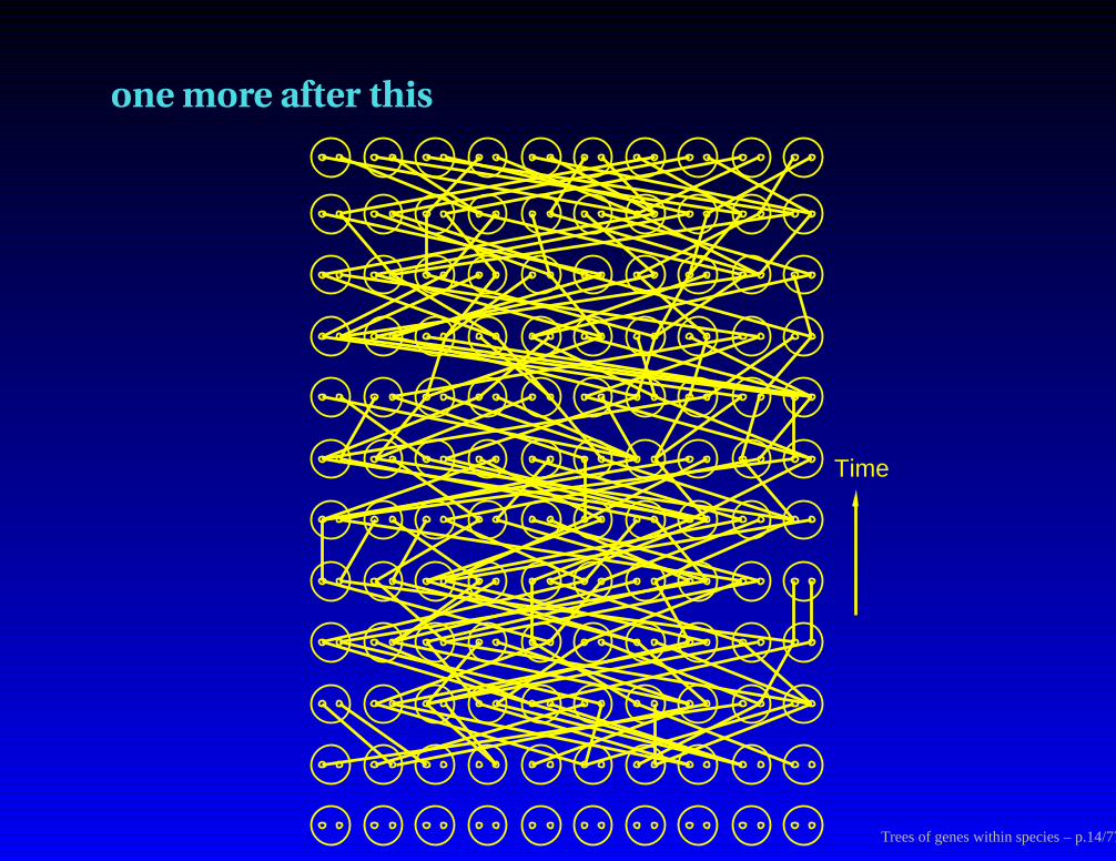
one more after this
Time
Trees of genes within species – p.14/77
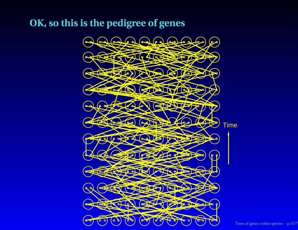
OK, so this is the pedigree of genes
Time
Trees of genes within species – p.15/77

The ancestry of gene copies, untangled
Time
Genealogy of gene copies, after reordering the copies
Trees of genes within species – p.16/77

The ancestry of a sample of 3 genes
Time
Trees of genes within species – p.17/77
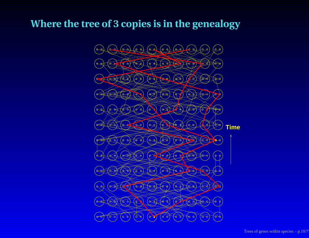
Where the tree of 3 copies is in the genealogy
Time
Trees of genes within species – p.18/77

Kingman’s coalescent process
u9
u7
u5
u3
u8
u6
u4
u2
Random collision of lineages as go back in time (sans recombination)Collision is faster the smaller the effective population size
Average time for n
Average time for
copies to coalesce to
4N
k(k−1) k−1 =
In a diploid population of
effective population size N,
copies to coalesce
= 4N (1 − 1n (
generations
k
Average time for
two copies to coalesce
= 2N generations
Trees of genes within species – p.19/77
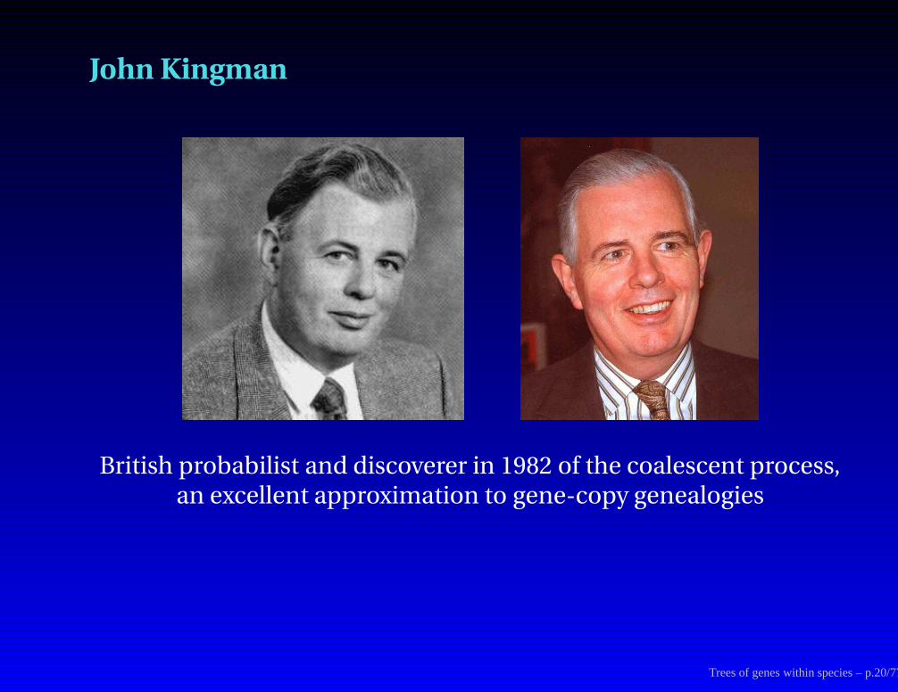
John Kingman
British probabilist and discoverer in 1982 of the coalescent process,an excellent approximation to gene-copy genealogies
Trees of genes within species – p.20/77
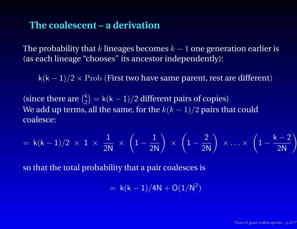
The coalescent – a derivation
The probability that k lineages becomes k − 1 one generation earlier is
(as each lineage “chooses" its ancestor independently):
k(k − 1)/2 × Prob (First two have same parent, rest are different)
(since there are(k2
)= k(k − 1)/2 different pairs of copies)
We add up terms, all the same, for the k(k − 1)/2 pairs that could
coalesce:
= k(k − 1)/2 × 1 ×1
2N×
(
1 −1
2N
)
×
(
1 −2
2N
)
× . . . ×
(
1 −k − 2
2N
)
so that the total probability that a pair coalesces is
= k(k − 1)/4N + O(1/N2)
Trees of genes within species – p.21/77
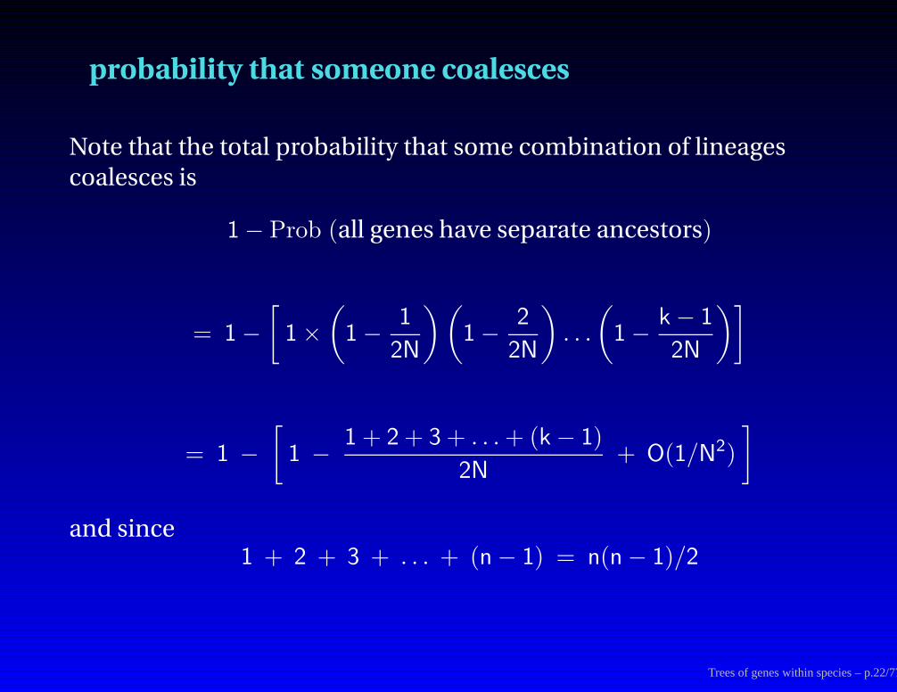
probability that someone coalesces
Note that the total probability that some combination of lineages
coalesces is
1 − Prob (all genes have separate ancestors)
= 1 −
[
1 ×
(
1 −1
2N
)(
1 −2
2N
)
. . .
(
1 −k − 1
2N
)]
= 1 −
[
1 −1 + 2 + 3 + . . . + (k − 1)
2N+ O(1/N2)
]
and since1 + 2 + 3 + . . . + (n − 1) = n(n − 1)/2
Trees of genes within species – p.22/77
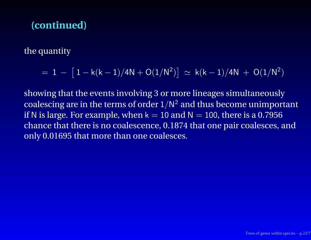
(continued)
the quantity
= 1 −[1 − k(k − 1)/4N + O(1/N2)
]' k(k − 1)/4N + O(1/N2)
showing that the events involving 3 or more lineages simultaneously
coalescing are in the terms of order 1/N2 and thus become unimportant
if N is large. For example, when k = 10 and N = 100, there is a 0.7956chance that there is no coalescence, 0.1874 that one pair coalesces, andonly 0.01695 that more than one coalesces.
Trees of genes within species – p.23/77

More rigorously ...
We get the coalescent as the limit when we start with k copies and passthrough a series of Markov processes, each with population size N, with
N → ∞
µ → 0 3 Nµ constant
(and similarly for other forces such as migration, growth, andrecombination rates)
with time in each process measured so that 1 unit is N generations
In fact, these are exactly the same conditions for obtaining the standardpopulation genetics diffusion approximations by weak convergence of
the Markov processes to the diffusion process.
Trees of genes within species – p.24/77

Accuracy with different population sizes
101 102 103 1040.0
0.2
0.4
0.6
0.8
population size
frac
tion
of tw
o−w
ay c
oale
scen
ces
(when sample size = 10)
Trees of genes within species – p.25/77
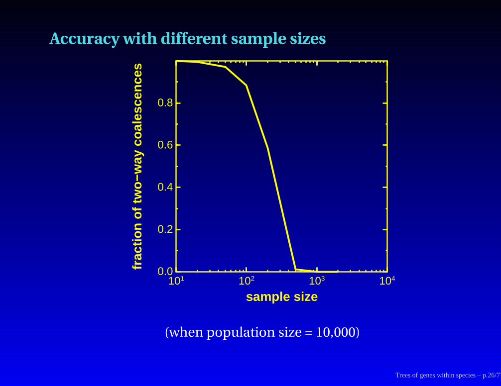
Accuracy with different sample sizes
101 102 103 1040.0
0.2
0.4
0.6
0.8
frac
tion
of tw
o−w
ay c
oale
scen
ces
sample size
(when population size = 10,000)
Trees of genes within species – p.26/77

Effect of varying population size
Ne
time
the changes in population size will produce waves of coalescence
time
Coalescence events
time
the tree
The parameters of the growth curve for Ne can be inferred bylikelihood methods as they affect the prior probabilities of those treesthat fit the data.
Trees of genes within species – p.27/77
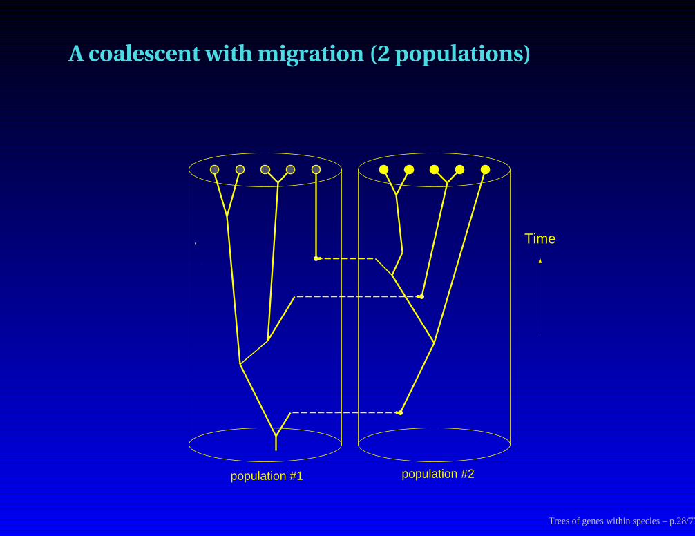
A coalescent with migration (2 populations)
Time
population #1 population #2
Trees of genes within species – p.28/77

A recombining coalescent
Recomb.
Different markers have slightly different coalescent trees
Trees of genes within species – p.29/77

Coalescents along a genome
1 142 143 417 418 562
Trees of genes within species – p.30/77

Their ancestral recombination graph
1−562 1−562 1−562 1−562
143−4171−142
418−562 1−417
1−142, 418−5621−562
1−562 1−562
Trees of genes within species – p.31/77
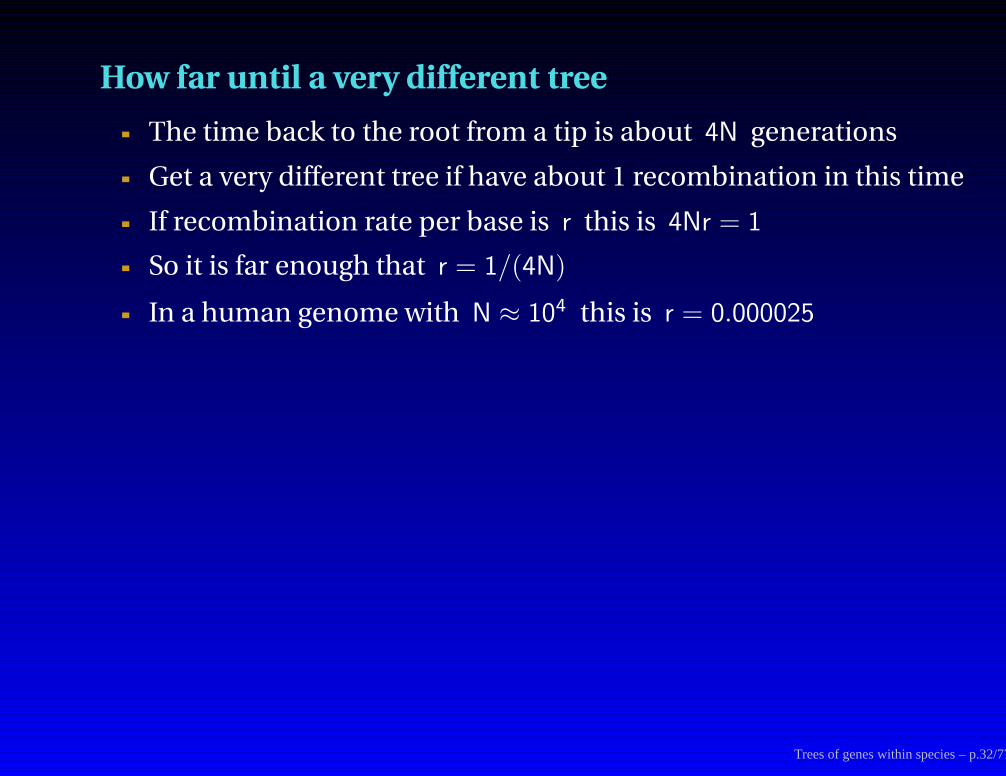
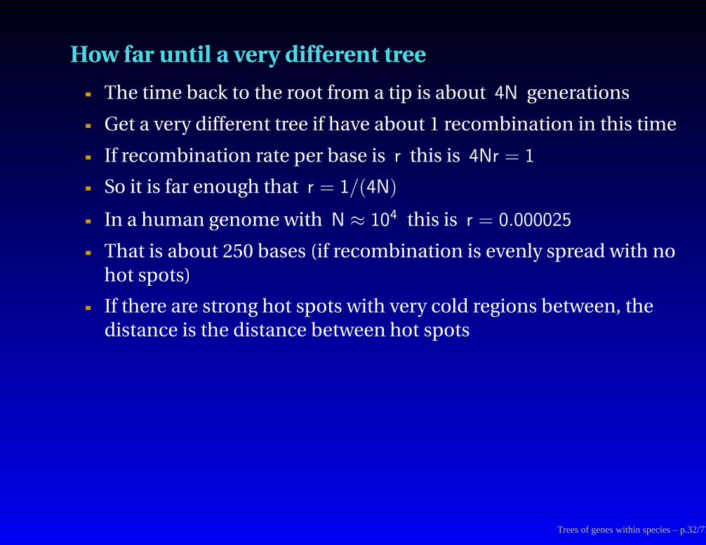
How far until a very different tree
The time back to the root from a tip is about 4N generations
Get a very different tree if have about 1 recombination in this time
If recombination rate per base is r this is 4Nr = 1
So it is far enough that r = 1/(4N)
In a human genome with N ≈ 104 this is r = 0.000025
That is about 250 bases (if recombination is evenly spread with no
hot spots)
If there are strong hot spots with very cold regions between, thedistance is the distance between hot spots
In any case no more than about 10 kb
So maybe about 320,000,000 different trees along the humangenome!
Trees of genes within species – p.32/77
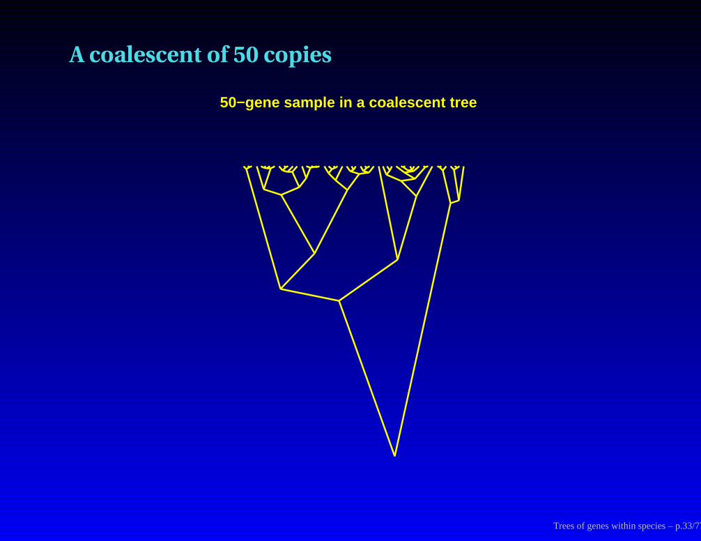
A coalescent of 50 copies
50−gene sample in a coalescent tree
Trees of genes within species – p.33/77

the first 10 copies only
10 gene copies in a coalescent tree
Trees of genes within species – p.34/77

All copies, ancestry of first 10 in orange
(orange lines are the 10−gene tree)
10 genes sampled randomly out of a 50−gene sample in a coalescent tree
Trees of genes within species – p.35/77

Some typical data with within-population variation
CAGTTTTAGCGTCC
CAGTTTTAGCGTCC
CAGTTTTAGCGTCC
CAGTTTTAGCGTCC
CAGTTTTAGCGTCC
CAGTTTTAGCGTCC
CAGTTTTAGCGTCC
CAGTTTTAGCGTCC
CAGTTTTAGCGTCC
CAGTTTTAGCGTCC
CAGTTTTAGCGTCC
CAGTTTCAGCGTCC
CAGTTTCAGCGTCC
CAGTTTCAGCGTCCCAGTTTCAGCGTCC
CAGTTTCAGCGTCC
CAGTTTCAGCGTCC
CAGTTTCAGCGTCC
CAGTTTCAGCGTCC
CAGTTTTGGCGTCC
CAGTTTTGGCGTCCCAGTTTTGGCGTCC
CAGTTTTGGCGTCC
CAGTTTTGGCGTCC
CAGTTTCAGCGTAC
CAGTTTCAGCGTAC
CAGTTTCAGCGTAC
, CAGTTTCAGCGTCC CAGTTTCAGCGTCC ), ... L = Prob ( = ??
To infer parameters of evolutionary−genetic models
With few exceptions, no expressions for this likelihood exist.
... we need to compute the likelihood for a set of genotypes sampled from a population
Trees of genes within species – p.36/77
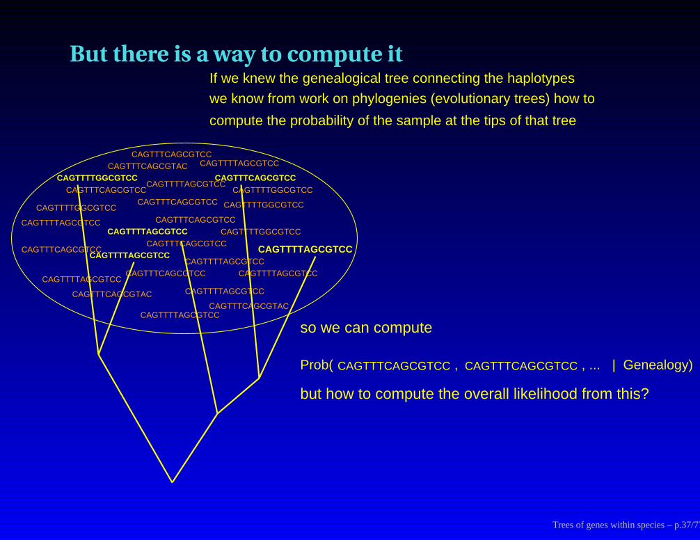
But there is a way to compute it
, CAGTTTCAGCGTCC CAGTTTCAGCGTCCProb( | Genealogy)
so we can compute
, ...
but how to compute the overall likelihood from this?
CAGTTTTAGCGTCC
CAGTTTTAGCGTCC
CAGTTTTAGCGTCC
CAGTTTTAGCGTCC
CAGTTTTAGCGTCC
CAGTTTTAGCGTCC
CAGTTTTAGCGTCC
CAGTTTTAGCGTCC
CAGTTTCAGCGTCC
CAGTTTCAGCGTCC
CAGTTTCAGCGTCC
CAGTTTCAGCGTCC
CAGTTTCAGCGTCC
CAGTTTCAGCGTCC
CAGTTTTGGCGTCCCAGTTTTGGCGTCC
CAGTTTTGGCGTCC
CAGTTTTGGCGTCC
CAGTTTCAGCGTACCAGTTTCAGCGTAC
CAGTTTCAGCGTAC
CAGTTTCAGCGTCC
CAGTTTTAGCGTCC
CAGTTTTAGCGTCC
CAGTTTTAGCGTCC
CAGTTTCAGCGTCCCAGTTTTGGCGTCC
we know from work on phylogenies (evolutionary trees) how to
compute the probability of the sample at the tips of that tree
If we knew the genealogical tree connecting the haplotypes
Trees of genes within species – p.37/77
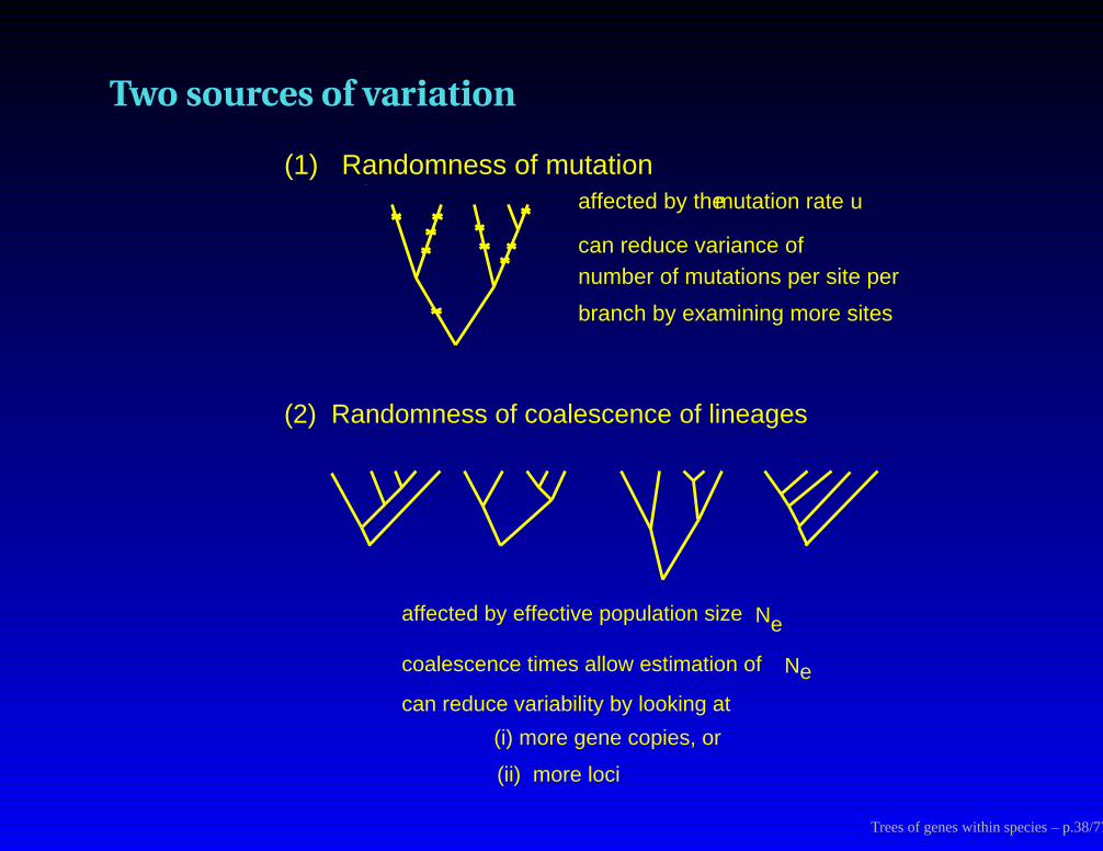
Two sources of variation
Ne
Ne
can reduce variability by looking at
(i) more gene copies, or
(ii) more loci
(2) Randomness of coalescence of lineages
affected by the
can reduce variance of
branch by examining more sites
number of mutations per site per
mutation rate u
(1) Randomness of mutation
affected by effective population size
coalescence times allow estimation of
Trees of genes within species – p.38/77

The basic equation for coalescent likelihoods
In the case of a single population with parameters
Ne effective population sizeµ mutation rate per site
and assuming G′ stands for a coalescent genealogy and D for the
sequences,
L = Prob (D |Ne, µ)
=∑
G′
Prob (G′ |Ne) Prob (D |G′, µ)
︸ ︷︷ ︸ ︸ ︷︷ ︸
Kingman′s prior likelihood of treeTrees of genes within species – p.39/77
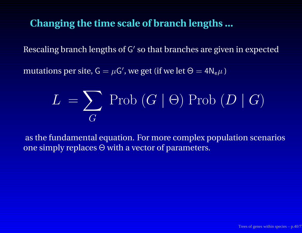
Changing the time scale of branch lengths ...
Rescaling branch lengths of G′ so that branches are given in expected
mutations per site, G = µG′, we get (if we let Θ = 4Neµ )
L =∑
G
Prob (G | Θ) Prob (D | G)
as the fundamental equation. For more complex population scenariosone simply replaces Θ with a vector of parameters.
Trees of genes within species – p.40/77
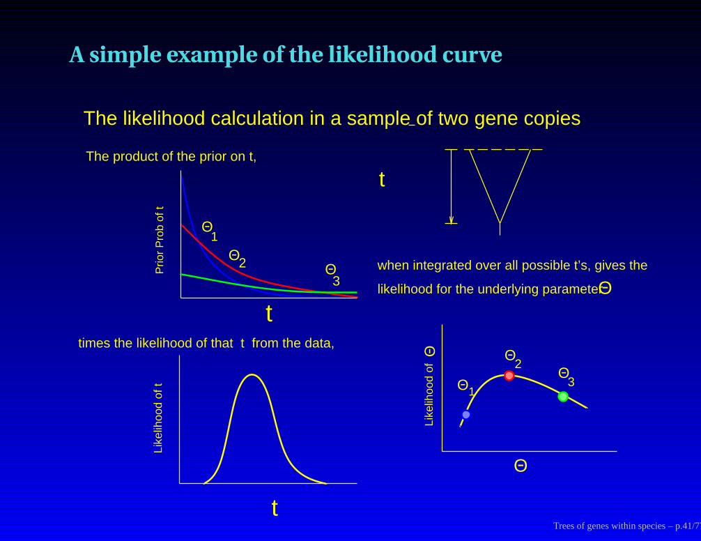
A simple example of the likelihood curve
t
t
Like
lihoo
d of
t
Like
lihoo
d of
The product of the prior on t,
times the likelihood of that t from the data,
when integrated over all possible t’s, gives the
likelihood for the underlying parameter
The likelihood calculation in a sample of two gene copies
t
1Θ2
Θ
3Θ
Θ
Prio
r P
rob
of t
2Θ
3Θ
Θ1
Θ
Θ
Trees of genes within species – p.41/77
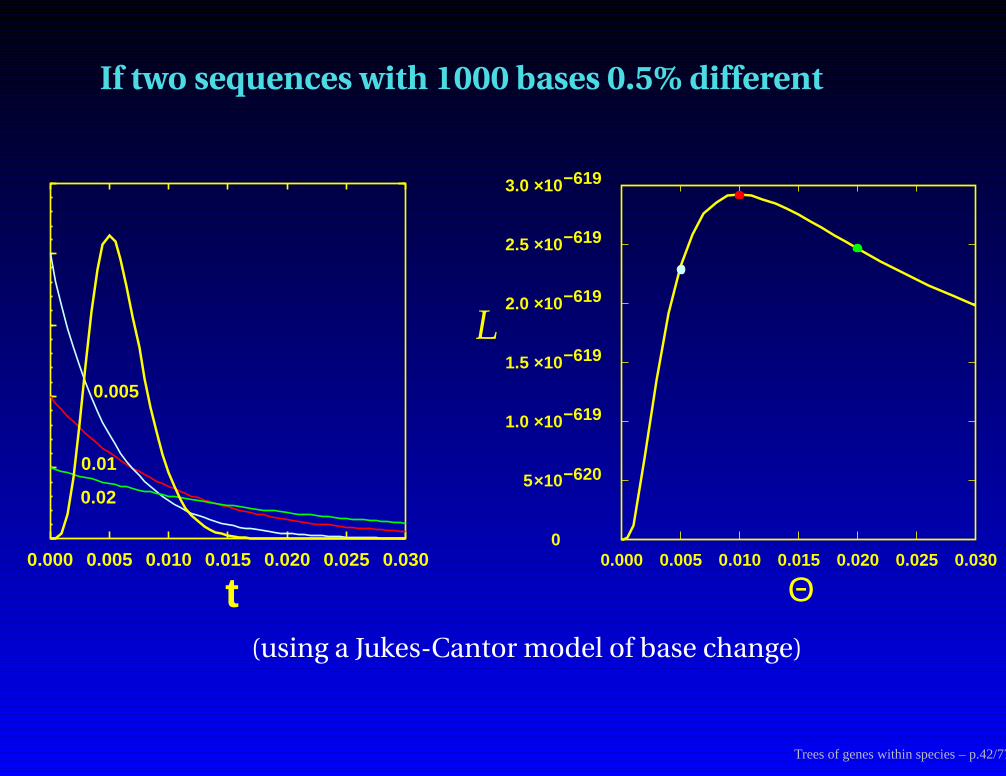
If two sequences with 1000 bases 0.5% different
0.000 0.005 0.010 0.015 0.020 0.025 0.030
0.005
0.01
0.02
t0.000 0.005 0.010 0.015 0.020 0.025 0.030
0
2.5 ×10−619
2.0 ×10−619
1.5 ×10−619
1.0 ×10−619
5×10−620
3.0 ×10−619
Θ
L
(using a Jukes-Cantor model of base change)
Trees of genes within species – p.42/77
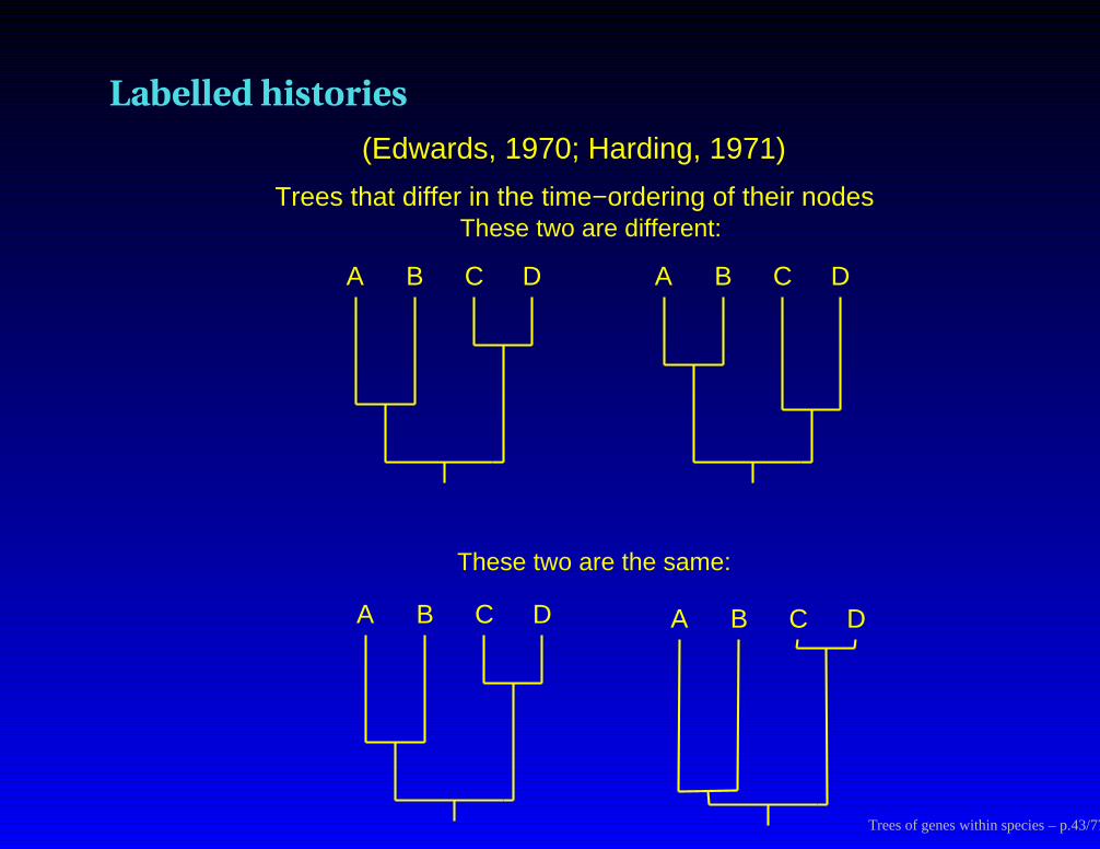
Labelled histories
Trees that differ in the time−ordering of their nodes
A B C D
A B C D
These two are the same:
A B C D
A B C D
These two are different:
(Edwards, 1970; Harding, 1971)
Trees of genes within species – p.43/77
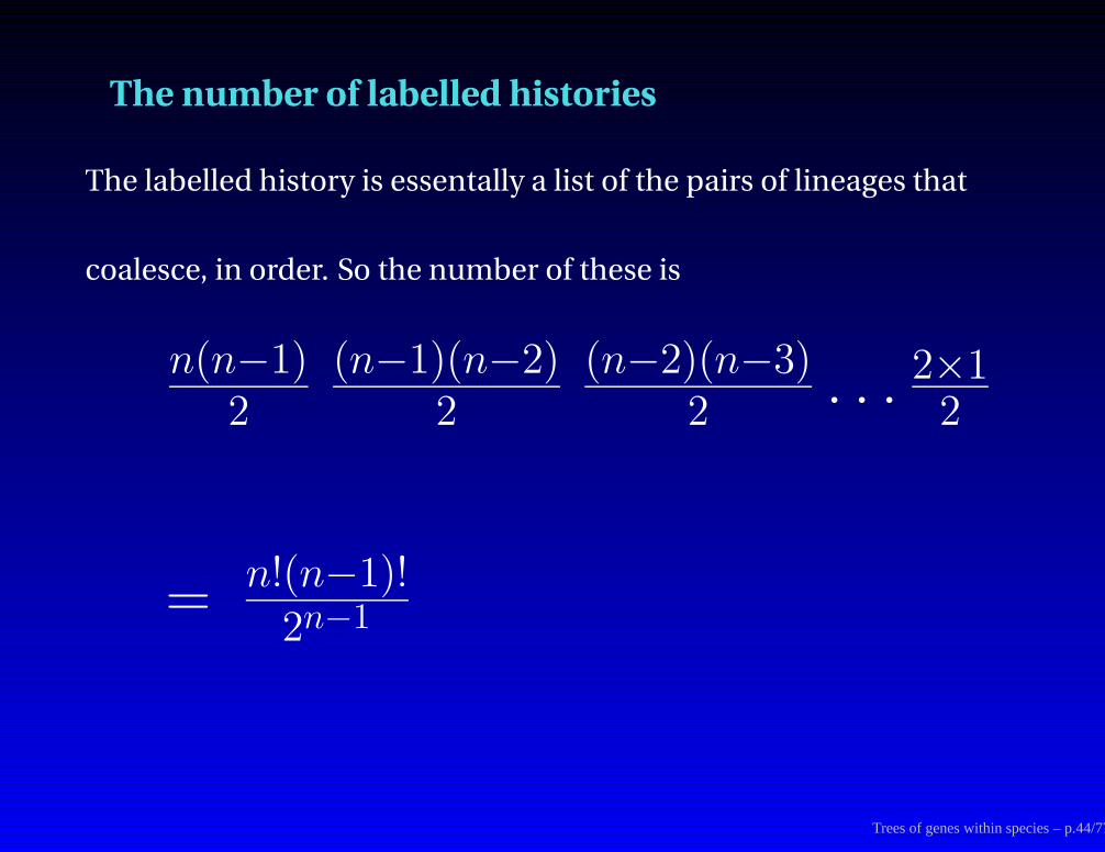
The number of labelled histories
The labelled history is essentally a list of the pairs of lineages that
coalesce, in order. So the number of these is
n(n−1)2
(n−1)(n−2)2
(n−2)(n−3)2 . . . 2×1
2
= n!(n−1)!2n−1
Trees of genes within species – p.44/77
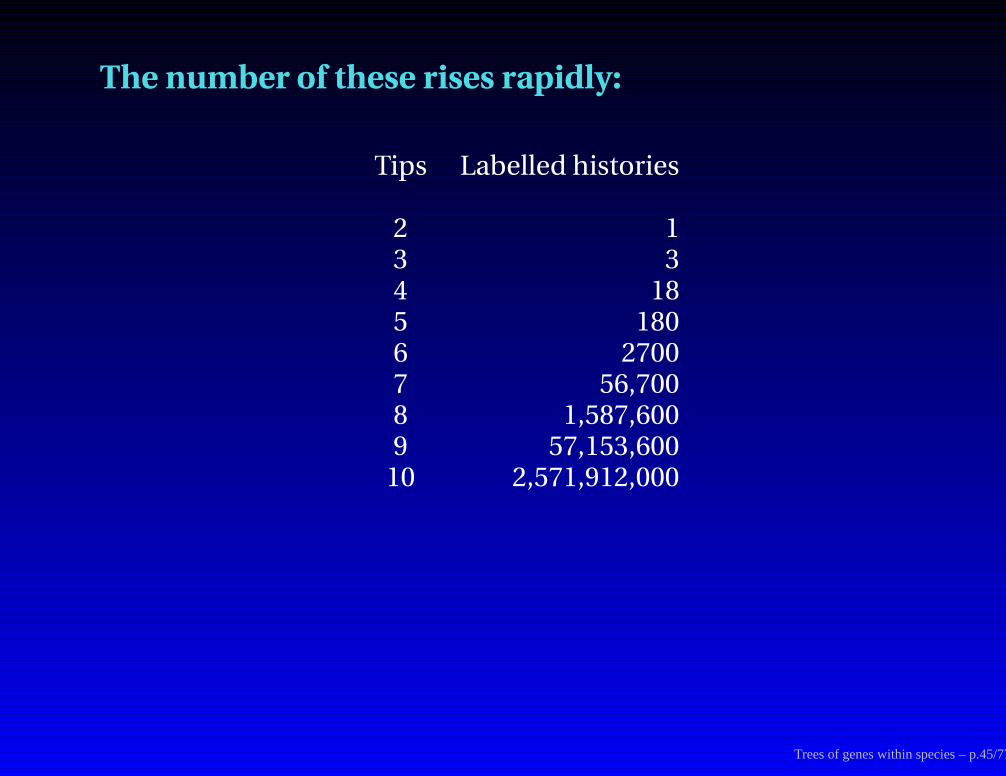
The number of these rises rapidly:
Tips Labelled histories
2 13 34 185 1806 27007 56,7008 1,587,6009 57,153,600
10 2,571,912,000
Trees of genes within species – p.45/77
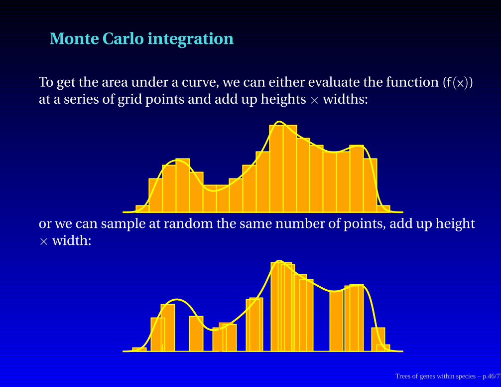
Monte Carlo integration
To get the area under a curve, we can either evaluate the function (f(x))
at a series of grid points and add up heights × widths:
or we can sample at random the same number of points, add up height× width:
Trees of genes within species – p.46/77
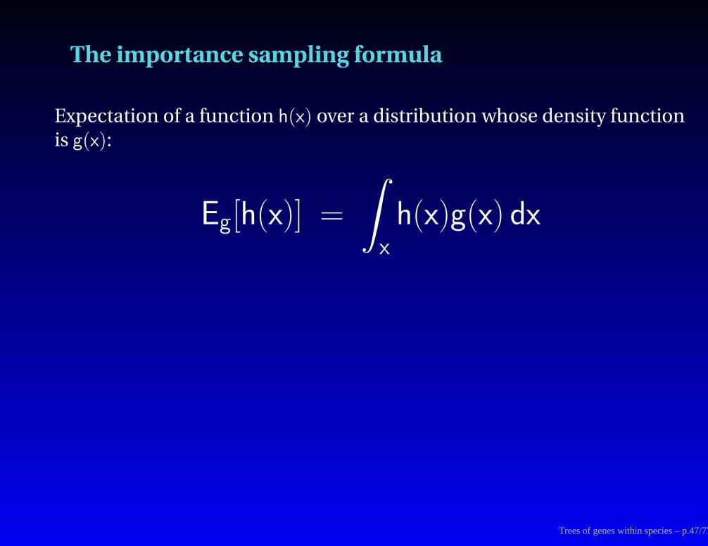
The importance sampling formula
Expectation of a function h(x) over a distribution whose density function
is g(x):
Eg[h(x)] =
∫
x
h(x)g(x) dx
Trees of genes within species – p.47/77
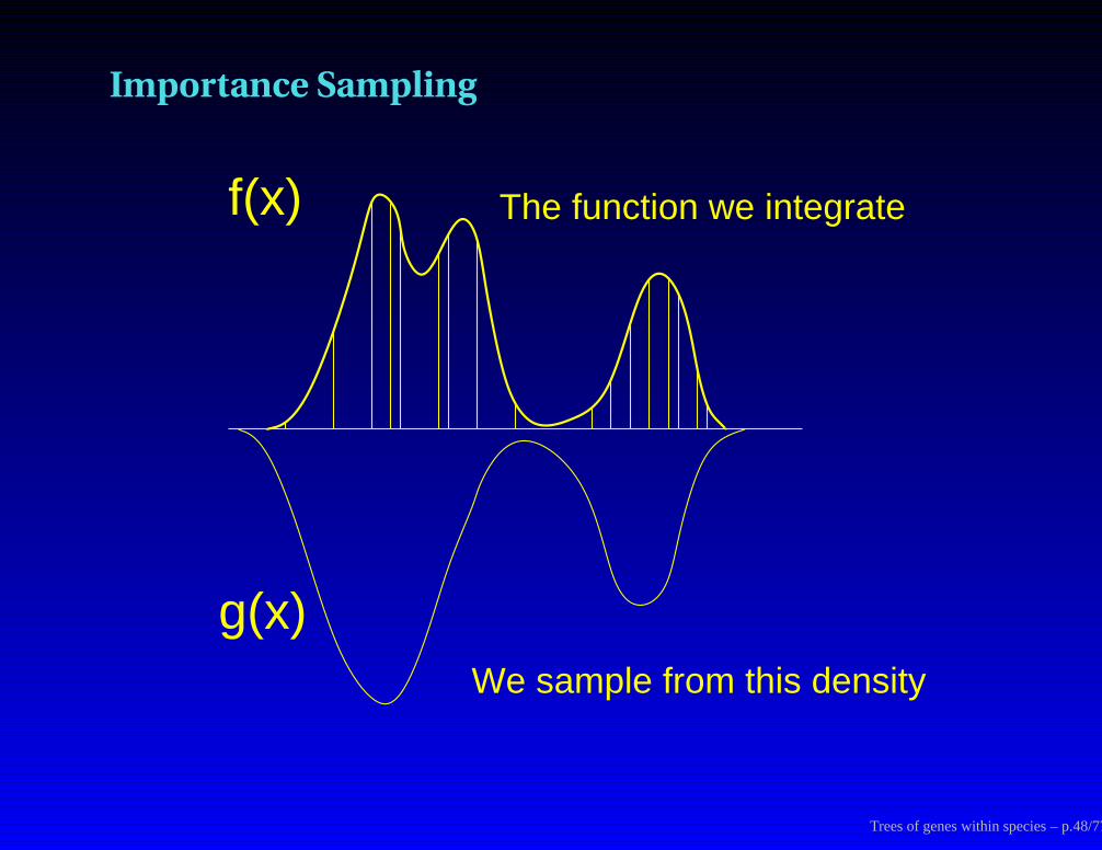
Importance Sampling
The function we integrate
We sample from this density
f(x)
g(x)
Trees of genes within species – p.48/77
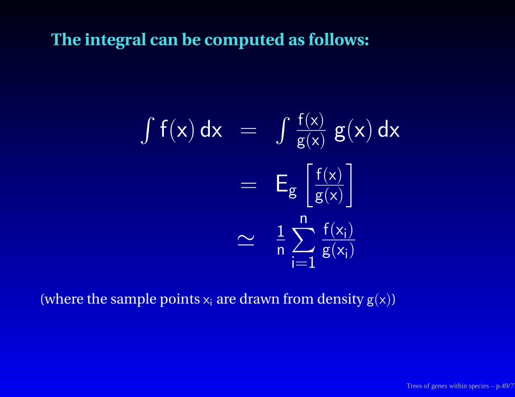
The integral can be computed as follows:
∫f(x) dx =
∫f(x)g(x) g(x) dx
= Eg
[f(x)g(x)
]
' 1n
n∑
i=1
f(xi)g(xi)
(where the sample points xi are drawn from density g(x))
Trees of genes within species – p.49/77
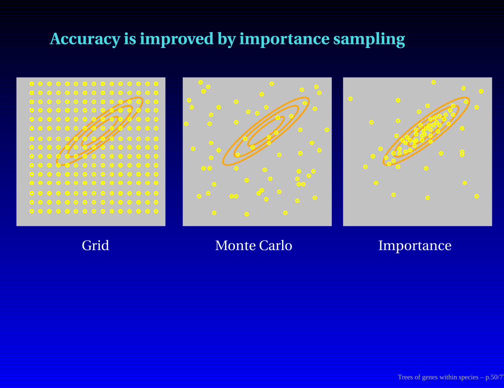
Accuracy is improved by importance sampling
Grid Monte Carlo Importance
Trees of genes within species – p.50/77
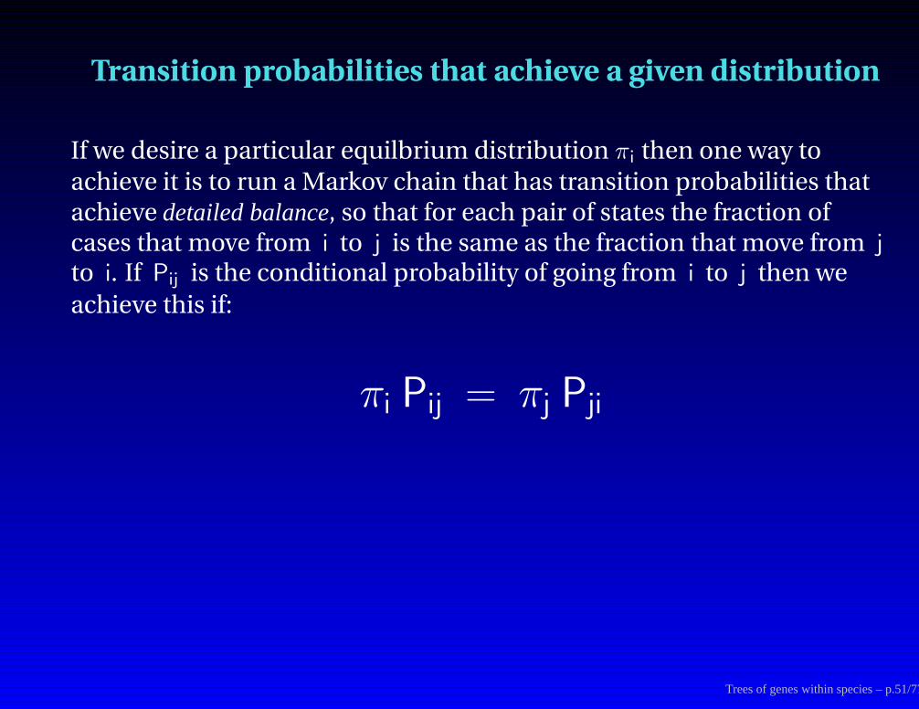
Transition probabilities that achieve a given distribution
If we desire a particular equilbrium distribution πi then one way to
achieve it is to run a Markov chain that has transition probabilities thatachieve detailed balance, so that for each pair of states the fraction ofcases that move from i to j is the same as the fraction that move from j
to i. If Pij is the conditional probability of going from i to j then we
achieve this if:
πi Pij = πj Pji
Trees of genes within species – p.51/77
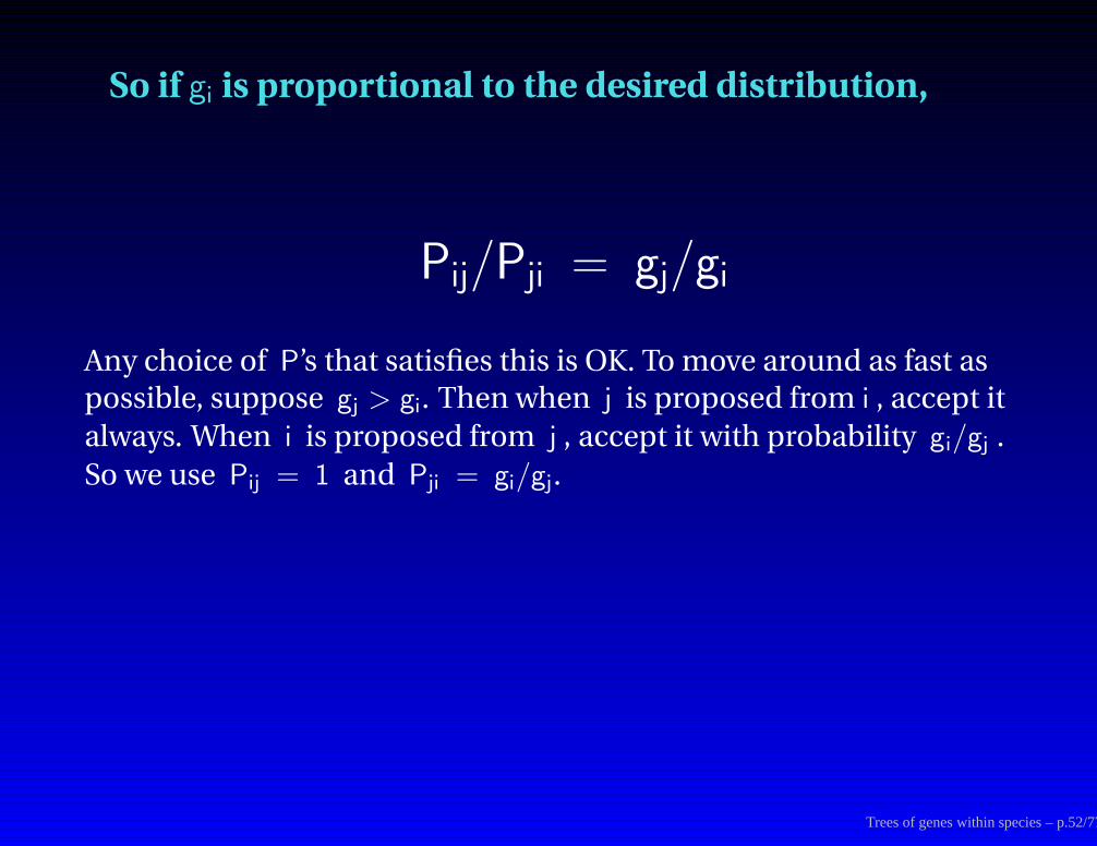
So if gi is proportional to the desired distribution,
Pij/Pji = gj/gi
Any choice of P’s that satisfies this is OK. To move around as fast as
possible, suppose gj > gi. Then when j is proposed from i , accept it
always. When i is proposed from j , accept it with probability gi/gj .
So we use Pij = 1 and Pji = gi/gj.
Trees of genes within species – p.52/77

MCMC: The Metropolis-Hastings method
To draw a sample G1, . . . , Gn from a distribution proportional to afunction g(G):
(1) Draw a change in G from some “proposal distribution": x → y
(2a) (Metropolis et. al., 1953):Accept the change if a uniformly-distributed random number R
satisfies
R <g(y)
g(x)
(2b) Hastings (Biometrika, 1970) corrected for biases toward some y ’s inthe proposal distribution by using instead
R <Prob(x|y)
Prob(y|x)
g(y)
g(x)
Repeat many times. If we do this long enough, and various nicenessconditions hold, then G1, . . . , Gm will be a sample from the right
distribution.Trees of genes within species – p.53/77
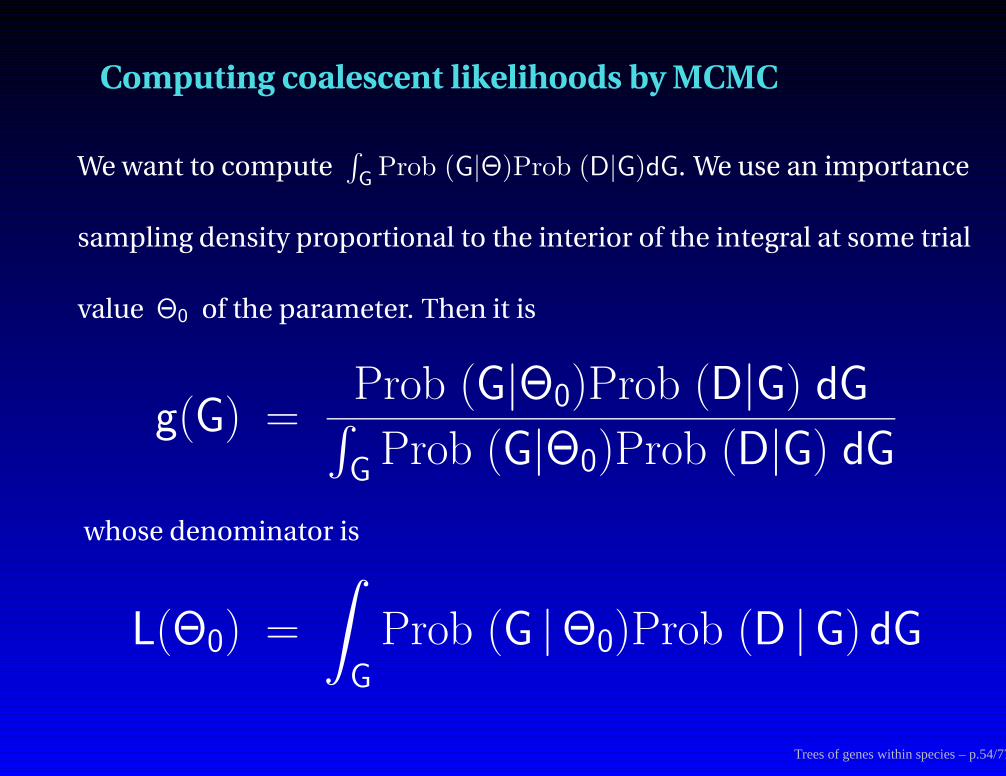
Computing coalescent likelihoods by MCMC
We want to compute∫
GProb (G|Θ)Prob (D|G)dG. We use an importance
sampling density proportional to the interior of the integral at some trial
value Θ0 of the parameter. Then it is
g(G) =Prob (G|Θ0)Prob (D|G) dG∫
GProb (G|Θ0)Prob (D|G) dG
whose denominator is
L(Θ0) =
∫
G
Prob (G |Θ0)Prob (D |G) dG
Trees of genes within species – p.54/77

The integral is:
L(Θ) ' 1n
n∑
i=1
f(Gi)g(Gi)
' 1n
n∑
i=1
Prob (G|Θ)Prob (D|G)Prob (G|Θ0)Prob (D|G)/L(Θ0)
This leads to
L(Θ)
L(Θ0)'
1
n
n∑
i=1
f(Gi)
g(Gi)'
1
n
n∑
i=1
Prob (Gi|Θ)
Prob (Gi|Θ0)
Trees of genes within species – p.55/77
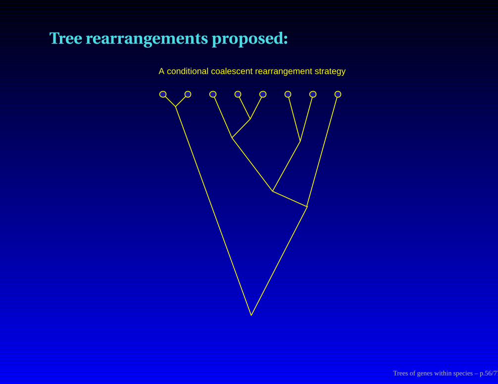
Tree rearrangements proposed:
A conditional coalescent rearrangement strategy
Trees of genes within species – p.56/77

more ...
First pick a random node (interior or tip) and remove its subtree
Trees of genes within species – p.57/77
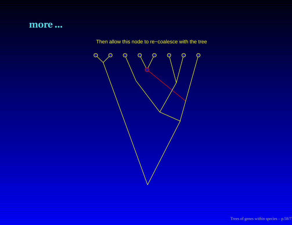
more ...
Then allow this node to re−coalesce with the tree
Trees of genes within species – p.58/77
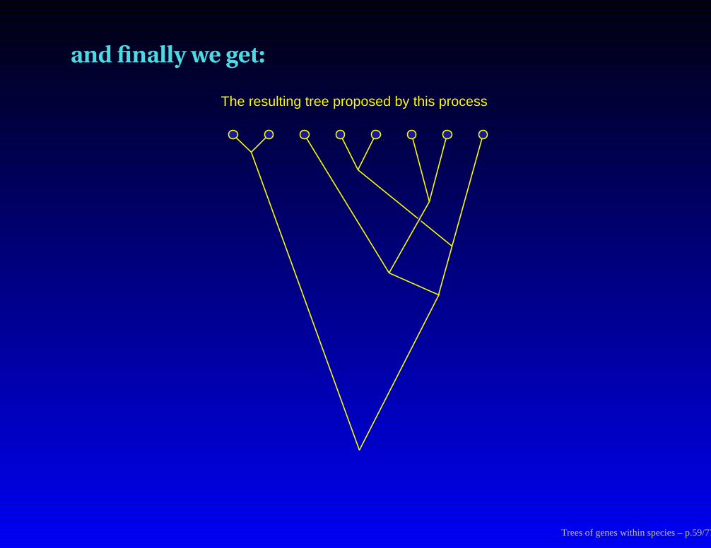
and finally we get:
The resulting tree proposed by this process
Trees of genes within species – p.59/77
Being left out of the story:
We choose the rearrangements so that the proposal distribution is
a “conditional coalescent".
We do a Hastings correction given this.
The end result is a perfect cancellation (which is pleasant ratherthan essential).
This leaves us with the rule that we use Prob (D |G) as the only
function in the Metropolizing.
Trees of genes within species – p.60/77
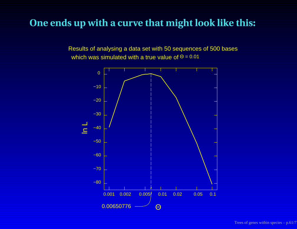
One ends up with a curve that might look like this:
0
−10
−20
−30
−40
−50
−60
−70
−80
0.001 0.002 0.005 0.01 0.02 0.05 0.1
Θ
ln L
0.00650776
Results of analysing a data set with 50 sequences of 500 baseswhich was simulated with a true value of Θ = 0.01
Trees of genes within species – p.61/77
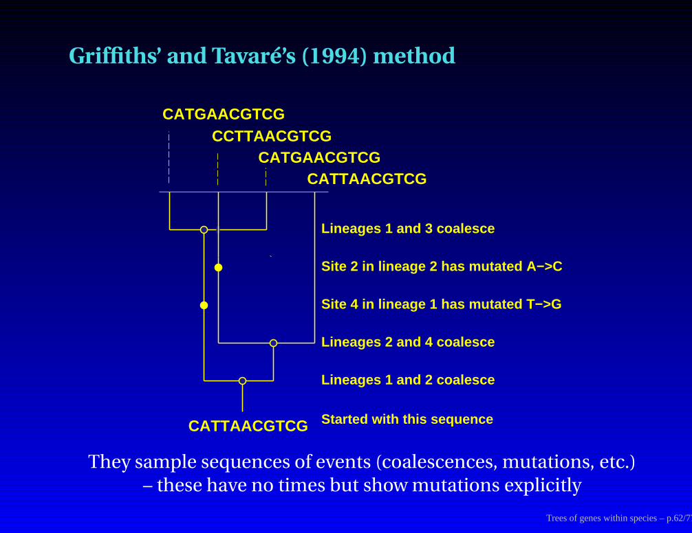
Griffiths’ and Tavaré’s (1994) method
CATTAACGTCGCATGAACGTCG
CCTTAACGTCGCATGAACGTCG
Lineages 1 and 3 coalesce
Lineages 1 and 2 coalesce
Lineages 2 and 4 coalesce
CATTAACGTCG Started with this sequence
Site 2 in lineage 2 has mutated A−>C
Site 4 in lineage 1 has mutated T−>G
They sample sequences of events (coalescences, mutations, etc.)– these have no times but show mutations explicitly
Trees of genes within species – p.62/77
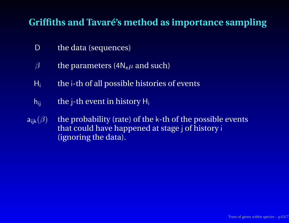
Griffiths and Tavaré’s method as importance sampling
D the data (sequences)
β the parameters (4Neµ and such)
Hi the i-th of all possible histories of events
hij the j-th event in history Hi
aijk(β) the probability (rate) of the k-th of the possible eventsthat could have happened at stage j of history i(ignoring the data).
Trees of genes within species – p.63/77
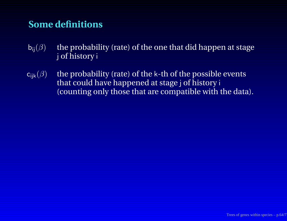
Some definitions
bij(β) the probability (rate) of the one that did happen at stagej of history i
cijk(β) the probability (rate) of the k-th of the possible eventsthat could have happened at stage j of history i(counting only those that are compatible with the data).
Trees of genes within species – p.64/77
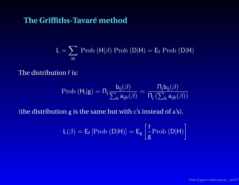
The Griffiths-Tavaré method
L =∑
H
Prob (H|β) Prob (D|H) = Ef Prob (D|H)
The distribution f is:
Prob (Hi|g) = Πj
bij(β)∑
k aijk(β)=
Πjbij(β)
Πj (∑
k aijk(β))
(the distribution g is the same but with c’s instead of a’s).
L(β) = Ef [Prob (D|H)] = Eg
[f
gProb (D|H)
]
Trees of genes within species – p.65/77

We end up with
L(β) = Eg
(
Πjbij(β)
Πj(∑
k aijk(β))
)
(
Πjbij(β0)
Πj(∑
k cijk(β0))
)
= Eg
[
Πj
(bij(β)
bij(β0)
)
Πj
(∑k cijk(β0)
∑
k aijk(β)
)]
Trees of genes within species – p.66/77
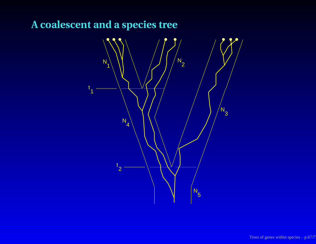
A coalescent and a species tree
t1
t2
N1
N2
N4
N3
N5
Trees of genes within species – p.67/77
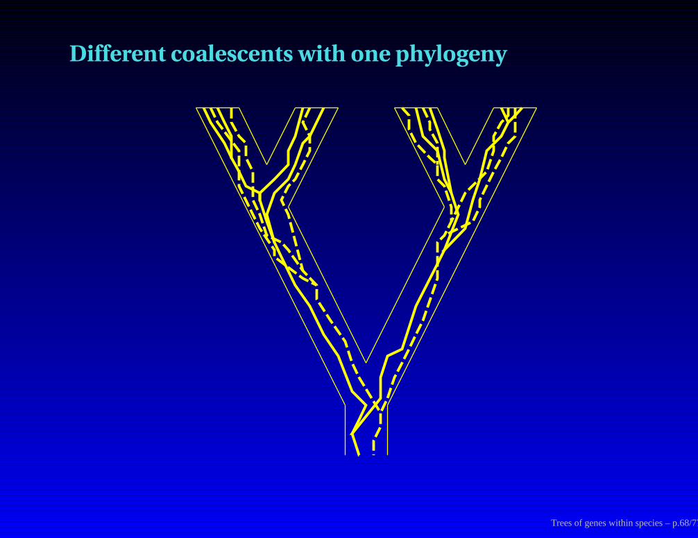
Different coalescents with one phylogeny
Trees of genes within species – p.68/77
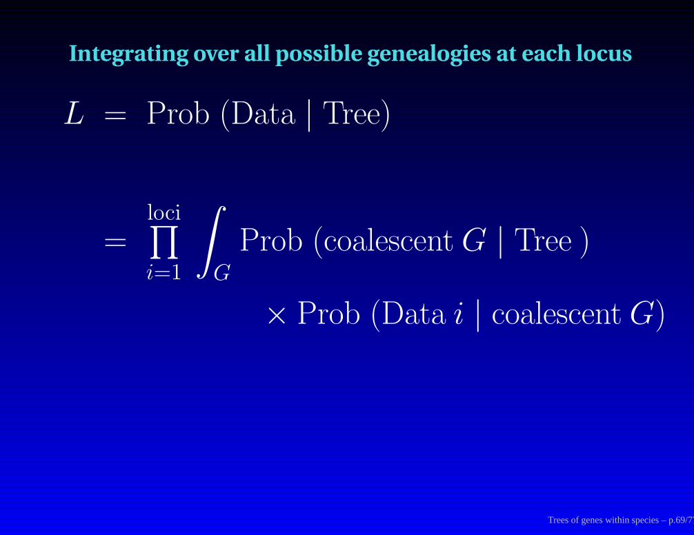
Integrating over all possible genealogies at each locus
L = Prob (Data | Tree)
=loci∏
i=1
∫
G
Prob (coalescent G | Tree )
× Prob (Data i | coalescent G)
Trees of genes within species – p.69/77
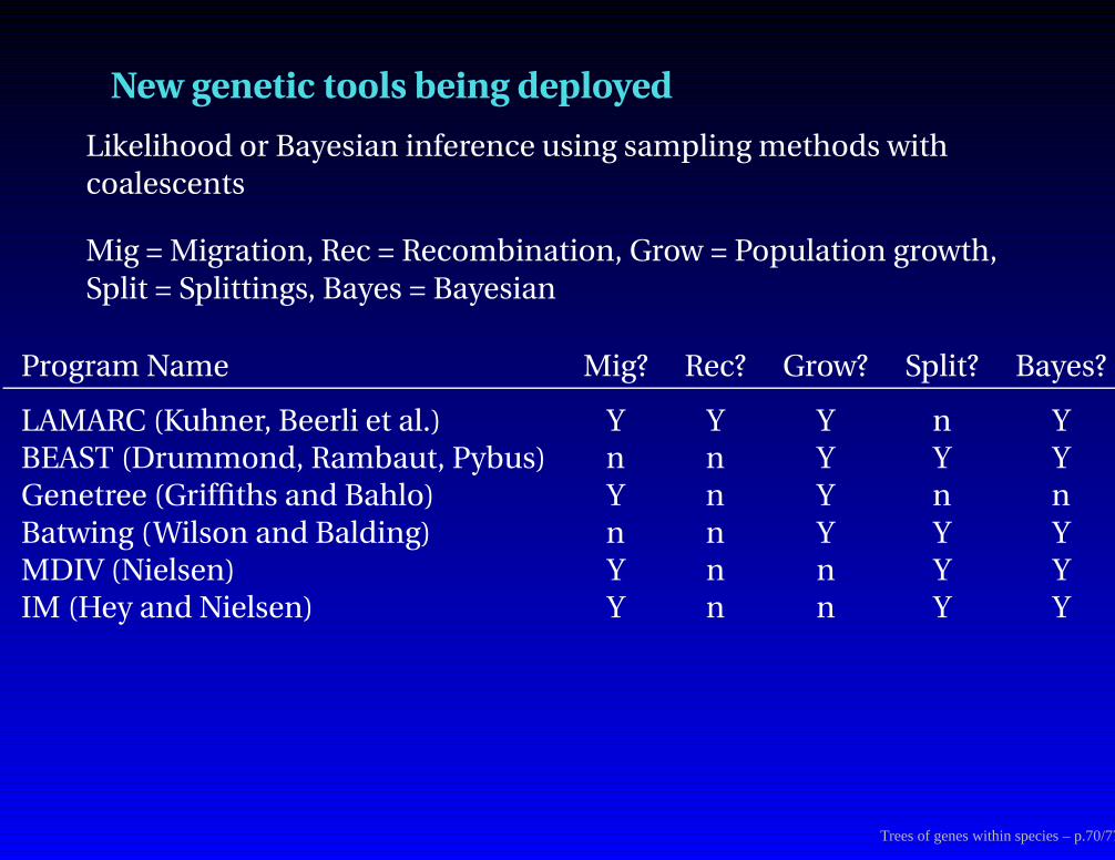
New genetic tools being deployed
Likelihood or Bayesian inference using sampling methods withcoalescents
Mig = Migration, Rec = Recombination, Grow = Population growth,
Split = Splittings, Bayes = Bayesian
Program Name Mig? Rec? Grow? Split? Bayes?
LAMARC (Kuhner, Beerli et al.) Y Y Y n YBEAST (Drummond, Rambaut, Pybus) n n Y Y YGenetree (Griffiths and Bahlo) Y n Y n nBatwing (Wilson and Balding) n n Y Y YMDIV (Nielsen) Y n n Y YIM (Hey and Nielsen) Y n n Y Y
Trees of genes within species – p.70/77
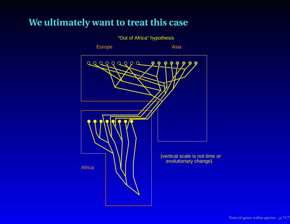
We ultimately want to treat this case
Africa
Europe Asia
"Out of Africa" hypothesis
(vertical scale is not time or evolutionary change)
Trees of genes within species – p.71/77
References
Beerli, P. B. and J. Felsenstein. 1999. Maximum-likelihood estimation ofmigration rates and effective population numbers in two populationsusing a coalescent approach. Genetics 152: 763-773. [Our approach tomigration estimation]
Edwards, A. W. F. 1970. Estimation of the branch points of a branching
diffusion process. Journal of the Royal Statistical Society B 32: 155-174.[Labelled histories]
Felsenstein, J. 1971. The rate of loss of multiple alleles in finite haploidpopulations. Theoretical Population Biology 2: 391-403. [Can be used toderive rates of coalescence]
Felsenstein, J. 1992. Estimating effective population size from samples of
sequences: inefficiency of pairwise and segregating sites as compared to
phylogenetic estimates. Genetical Research 59: 139-147. [Suggests usingthe coalescents]
Trees of genes within species – p.72/77

References
Felsenstein, J., M. K. Kuhner, J. Yamato, and P. Beerli. 1999. Likelihoods oncoalescents: a Monte Carlo sampling approach to inferring parametersfrom population samples of molecular data. pp. 163-185 in Statistics inMolecular Biology and Genetics, ed. F. Seillier-Moiseiwitsch. IMS LectureNotes-Monograph Series, volume 33. Institute of Mathematical Statisticsand American Mathematical Society, Hayward, California. [Overview ofmy lab’s methods]
Griffiths, R. C. 1989. Genealogical tree probabilities in theinfinitely-many-site model. Journal of Mathematical Biology 27: 667-680.[Summing up over event histories]
Griffiths, R. C. and S. Tavaré. 1994a. Sampling theory for neutral alleles in avarying environment. Philosophical Transactions of the Royal Socety ofLondon, Series B (Biological Sciences) 344: 403-10. [Griffiths-Tavaresampling method]
Griffiths, R. C. and S. Tavaré. 1994b. Ancestral inference in populationgenetics. Statistical Science 9: 307-319. [Griffiths-Tavare sampling method]
Trees of genes within species – p.73/77

References
Griffiths, R. C. and P. Marjoram. 1996. Ancestral inferences from samples of
DNA sequences with recombination. Journal of Computational Biology 3:479-502. [Coalescent likelihoods with recombination]
Griffiths, R. C. and S. Tavaré. 1997. Computational methods for thecoalescent. pp. 165-182 in Progress in Population Genetics and HumanEvolution, ed. P. Donnelly and S. Tavaré. IMA Volumes on Mathematics
and Its Applications, volume 87. Springer, New York. [Review of theirapproach] Hastings, W. K. 1970. Monte Carlo sampling methods using
Markov chains and their applications. Biometrika 57: 97-109. [TheHastings correction]
Hein, J., M. H. Schierup, and C. Wiuf. 2005. Gene Genealogies, Variation, andEvolution. Oxford University Press, Oxford. [Then first book on thecoalescent, emphasizing its population genetics]
Hudson, R. R. and N. L. Kaplan. 1985. Statistical properties of the number ofrecombination events in the history of a sample of DNA sequences.Genetics 111: 147-164. [Coalescent with recombination]
Hudson, R. R. 1990. Gene genealogies and the coalescent process. OxfordSurveys in Evolutionary Biology 7: 1-44. [The first major review ofcoalescents] Trees of genes within species – p.74/77

References
Kingman, J. F. C. 1982a. The coalescent. Stochastic Processes and TheirApplications 13: 235-248. [One of the papers in which the coalescent isintroduced]
Kingman, J. F. C. 1982b. On the genealogy of large populations. Journal ofApplied Probability 19A: 27-43. [Another of the papers in which thecoalescent is introduced]
Krone, S. M. and C. Neuhauser. 1997. Ancestral processes with selection.Theoretical Population Biology 51: 210-237. [A very original extension of thecoalescent to allow selection]
Kuhner, M. K., J. Yamato, and J. Felsenstein. 1995. Effective population sizeand mutation rate from sequence data using Metropolis-Hastings
sampling. Genetics 140: 1421-1430. [Our MCMC coalescent likelihoodmethod]
Kuhner, M. K., J. Yamato, and J. Felsenstein 1997. Applications ofMetropolis-Hastings genealogy sampling. pp. 183-192 in Progress inPopulation Genetics and Human Evolution, ed. P. Donnelly and S. Tavare.
IMA Volumes in Mathematics and its Applications, volume 87. SpringerVerlag, Berlin. [Brief review of our approach]
Trees of genes within species – p.75/77
References
Kuhner, M. K., J. Yamato and J. Felsenstein. 1998. Maximum likelihoodestimation of population growth rates based on the coalescent Genetics149: 429-434. [Our approach to growing populations, and describes a bias inestimation]
Metropolis, N., A. W. Rosenbluth, M. N. Rosenbluth, A. H. Teller and E. Teller.1953. Equation of state calculations by fast computing machines. Journalof Chemical Physics 21: 1087-1092. [The Metropolis algorithm]
Neuhauser, C., and S. M. Krone. 1997. The genealogy of samples in models
with selection. Genetics 145: 519-534. [A very original extension of thecoalescent to allow selection]
Nielsen, R. 1997. Maximum likelihood estimation of population divergence
times and population phylogenies under the infinite sites model.Theoretical Population Biology 53: 143-151. [The first coalescent likelihoodpaper with more than one species]
Takahata, N. 1988. The coalescent in two partially isolated diffusion
populations. Genetical Research 52: 213-222. [Coalescents with migration]Wakeley, J. 2005. Coalescent Theory, an Introduction. Roberts and Co.,
Greenwood Village, Colorado. [Coming this summer – very readable, withemphasis on the population genetics] Trees of genes within species – p.76/77

How it was done
This projection produced as a PDF, not a PowerPoint file, and viewedusing the Full Screen mode (in the View menu of Adobe Acrobat Reader):
using the prosper style in LaTeX (prosper.sourceforge.net),
using Latex to make a .dvi file,
using dvips to turn this into a Postscript file,
using ps2pdf to make it into a PDF file, and
displaying the slides in Adobe Acrobat Reader.
Result: nice slides using freeware.
Trees of genes within species – p.77/77


