Gain and noise spectral density in an electronic parametric amplifier with
added white noise
Adriano A. Batista1 and A. A. Lisboa de Souza2
1 Departamento de Fısica, Universidade Federal de Campina Grande
Campina Grande-PB, CEP: 58109-970, Brazil2 Departamento de Engenharia Eletrica, Universidade Federal da Paraıba
Joao Pessoa-PB, CEP: 58.051-970, Brazil
(Dated: October 17, 2018)
Abstract
In this paper, we discuss the behavior of a linear classical parametric amplifier (PA) in the presence
of white noise and give theoretical estimates of the noise spectral density based on approximate Green’s
functions obtained by using averaging techniques. Furthermore, we give analytical estimates for parametric
amplification bandwidth of the amplifier and for the noisy precursors to instability. To validate our theory
we compare the analytical results with experimental data obtained in an analog circuit. We describe the
implementation details and the setup used in the experimental study of the amplifier. Near the threshold
to the first parametric instability, and in degenerate-mode amplification, the PA achieved very high gains
in a very narrow bandwidth centered on its resonance frequency. In quasi-degenerate mode amplification,
we obtained lower values of gain, but with a wider bandwidth that is tunable. The experimental data were
accurately described by the predictions of the model. Moreover, we noticed spectral components in the
output signal of the amplifier which are due to noise precursors of instability. The position, width, and
magnitude of these components are in agreement with the noise spectral density obtained by the theory
proposed here.
1
arX
iv:1
509.
0579
5v1
[ph
ysic
s.cl
ass-
ph]
4 S
ep 2
015
I. INTRODUCTION
Parametrically-driven systems and parametric resonance occur in many different physical sys-
tems, ranging from the mechanical domain to the electronic, microwave, electromechanic, op-
tomechanic, and quantum domains. In the mechanical domain we have Faraday waves [1], in-
verted pendulum stabilization, stability of boats, balloons, and parachutes [2]. A comprehensive
review of applications in electronics and microwave cavities spanning from the early twentieth
century up to 1960 can be found in Ref. [3]. A few relevant recent applications, in micro and nano
systems, include quadrupole ion guides and ion traps [4], linear ion crystals in linear Paul traps
designed as prototype systems for the implementation of quantum computing [5–7], magnetic
resonance force microscopy [8], tapping-mode force microscopy [9], axially-loaded microelec-
tromechanical systems (MEMS) [10, 11], torsional MEMS [12]. In the quantum domain we could
mention wideband superconducting parametric amplifiers [13], squeezing in optomechanical cav-
ities below the zero-point motion [14], and parametric amplification in Josephson junctions [15]
Parametric pumping has had many applications in the field of MEMS, which have been used pri-
marily as accelerometers, for measuring small forces and as ultrasensitive mass detectors since the
mid 80’s [16]. An enhancement to the detection techniques in MEMS was developed by Rugar
and Grutter [17] in the early 90’s that uses mechanical parametric amplification (before transduc-
tion) to improve the sensitivity of measurements. This amplification method works by driving the
parametrically-driven resonator on the verge of parametric unstable zones.
Here, we study a classical parametric amplifier both in theory and in experiment with analog
electronics. We investigate signal and idler responses near the onset of the first parametric instabil-
ity. We find the experimental results of gain in the signal and idler responses accurately described
by the theory. We also investigate the noisy precursors of instability. We provide an analytical
expression for the noise spectral density of a parametrically-driven oscillator with added noise.
Again, mostly, we have very good agreement between experiment and theoretical predictions.
The novelty compared with the work of Wiesenfeld et al. in the 80’s [18, 19] is that we provide
a simpler theoretical derivation for the noise spectral density (NSD) based on Green’s functions
and the averaging method, in which the contribution of both Floquet multipliers involved are taken
into account. Furthermore, we provide an analytical expression for the noise spectral density in
terms of the parameters of the system and not in terms of the largest Floquet multiplier, which
is left unspecified in their theory. The analytical calculation of the Floquet multipliers can still
2

be a daunting problem to overcome. Another difference, is that below threshold there is no pe-
riodic solution, the system is in quiescent mode, a system that was not treated by Wiesenfeld et
al.. Because we add noise to a linear parametrically-driven system below threshold, we can fit the
NSD when there is no pumping with the NSD of a harmonic oscillator with added noise and thus
calibrate the noise level. If we had used Wiesenfeld’s theory the measured noise level would be
off by 6dB. In their model there is always a parametric pumping, since the noise is treated as a
perturbation around a deterministic limit cycle of a nonlinear dynamical system. Hence, the pos-
sibility of calibration of the NSD around a harmonic oscillator limit is not possible, or at least is
not clear, in their theory.
The contents of this paper are organized as follows. In Sec. (II) we present our theoretical
model, in Sec. (III) we describe our experimental setup, in Sec. (IV) we present and discuss our
numerical and experimental results, and in Sec. (V) we draw our conclusions.
II. THEORY
The block diagram shown in Fig. 1 is an schematic implementation of an electronic circuit of
the parametric amplifier. The block with the × symbol in it represents a multiplier and the box
with a Σ symbol is a summer. The equation that describes this system is given by
LCd2Vcds2
+RCdVcds
+ Vc = AVp cos(4πfs)Vc + V0 cos(2πfss+ φ0), (1)
where Vc is the voltage on the capacitor, L is the inductance, C is the capacitance, R is the re-
sistance, Vp is the pump amplitude, A is the amplification factor of the multiplier (with units of
volt−1), V0 is the signal voltage amplitude, 2f is the pump frequency, fs is the frequency of the
signal, and φ0 is the phase of the signal. We can simplify Eq. (1) with the adimensional time
t = ω0s, where ω0 = 1/√LC, γ = 1/Q = R/(ω0L), Fp = AVp, F0 = V0. We find
d2x
dt2+ x = −γ dx
dt+ Fp cos(2ωt)x+ F0 cos(ωst+ φ0), (2)
where x(t) = Vc(t), ω = 2πf/ω0, and ωs = 2πfs/ω0.
3

A. The Green’s function of the parametric oscillator
The equation for the Green’s function of the parametrically-driven oscillator described in Eq. (2)
obeys [∂2
∂t2+ 1 + γ
∂
∂t− Fp cos(2ωt)
]G(t, t′) = δ(t− t′). (3)
We use the retarded Green’s function which is G(t, t′) = 0 for t < t′. By integrating the above
equation near t = t′, we obtain the initial conditions when t = t′ + 0+, which are G(t, t′) = 0
and ∂∂tG(t, t′) = 1.0. Assuming the parameters γ, Fp = O(ε), with 0 < ε << 1, we can write
the Green’s function in the stable zone of the parametrically-driven oscillator in the first-order
averaging approximation [20] as
G(t, t− τ) ≈ G0(τ) +Gp(t, τ), (4)
with
G0(τ) =e−γτ/2
ω
[cosh(κ τ) sin(ωτ) +
δ
κsinh(κ τ) cos(ωτ)
],
Gp(t, τ) = − β
ωκe−γτ/2 sinh(κ τ) cos(ω(2t− τ)).
where τ = t− t′ > 0, κ =√β2 − δ2, β = −Fp/4ω, and δ = Ω/2ω, and Ω = 1− ω2.
B. The ac-signal response in the parametric oscillator
Here we present the theory on classical linear parametric amplification near the onset of the first
instability zone of the parametric amplifier, i.e. we analyze the response of a parametric oscillator
to an added input ac signal. In the following, we will use the Green’s function of Eq. (4) to obtain
the solution of Eq. (2). This is given by
x(t) =
∫ t
−∞G(t, t′)F0 cos(ωst
′ + φ0) dt′, (5)
since we assume the pump and the input signal have been turned on for a long time, any homoge-
neous solution has already decayed. The signal response is given by∫ t
−∞dt′ G0(t− t′) cos(ωst
′ + φ0) = Re∫ t
−∞dt′ G0(t− t′)e−i(ωst′+φ0)
= Re[e−i(ωst+φ0)
∫ t
−∞dt′ G0(t− t′)eiωs(t−t′)
]= Re
[e−i(ωst+φ0)
∫ ∞0
G0(τ)eiωsτ
]= Re
[e−i(ωst+φ0)G0(ωs)
]. (6)
4

In order to obtain
G0(ωs) =
∫ ∞−∞
eiωstG0(t)dt
=1
ω
∫ ∞0
e−γt/2eiωst
[cosh(κ t) sin(ωt) +
δ
κsinh(κ t) cos(ωt)
]dt, (7)
the following integrals were utilized∫ ∞0
e[−γ/2+i(ωs±ω)]t cosh(κt)dt =γ − 2i(ωs + ω)
2[γ/2− κ− i(ωs ± ω)][γ/2 + κ− i(ωs ± ω)],∫ ∞
0
e[−γ/2+i(ωs±ω)]t sinh(κt)dt =κ
[γ/2− κ− i(ωs ± ω)][γ/2 + κ− i(ωs ± ω)],
and we obtained
G0(ωs) ≈1
ω
1
2i
[γ − 2i(ωs + ω)
2[γ/2− κ− i(ωs + ω)][γ/2 + κ− i(ωs + ω)]
− γ − 2i(ωs − ω)
2[γ/2− κ− i(ωs − ω)][γ/2 + κ− i(ωs − ω)]
]+δ
2
[1
[γ/2− κ− i(ωs + ω)][γ/2 + κ− i(ωs + ω)]
+1
[γ/2− κ− i(ωs − ω)][γ/2 + κ− i(ωs − ω)]
]. (8)
Hence, with the help of the appendix calculations, we find the stationary solution of Eq. (2) to
be approximately
x(t) ≈ F0
Re[e−i(ωst+φ0)G0(ωs)
]− β
2ωRe[
ei[(2ω+ωs)t+φ0]
[γ/2− κ+ i(ω + ωs)][γ/2 + κ+ i(ω + ωs)]
+ei[(2ω−ωs)t−φ0]
[γ/2− κ+ i(ω − ωs)][γ/2 + κ+ i(ω − ωs)]
]. (9)
With ωs ≈ ω and when the PA is pumped near the onset of the first instability, we find the idler
response to be∫ t
−∞dt′ Gp(t, t
′) cos(ωst′ + φ0) ≈ − β
2ωRe
ei[(2ω−ωs)t−φ0]
[γ/2− κ+ i(ω − ωs)][γ/2 + κ+ i(ω − ωs)]
.
We also find that the envelope of the time series x(t) given in Eq. (9) is approximately∣∣∣∣e−i[(ω−ωs)t−φ0]G∗0(ωs)−β
2ω
ei[(ω−ωs)t−φ0]
[γ/2− κ+ i(ω − ωs)][γ/2 + κ+ i(ω − ωs)]
∣∣∣∣ (10)
5
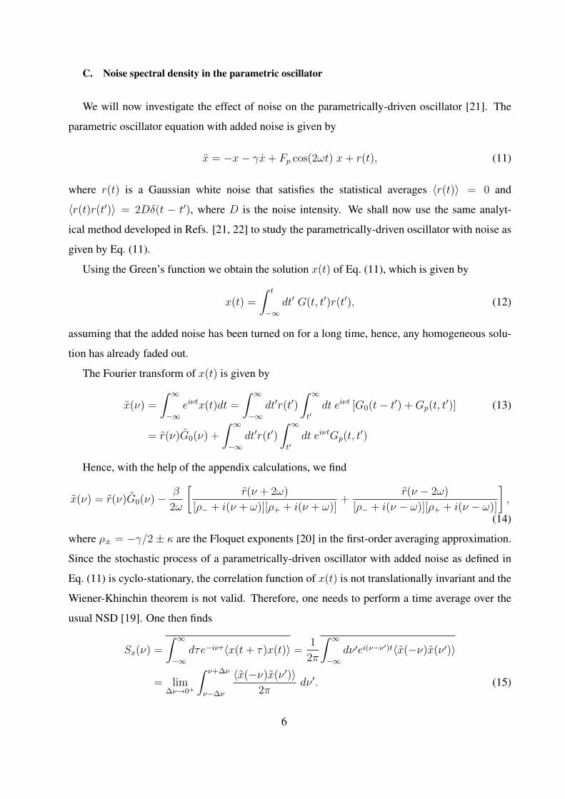
C. Noise spectral density in the parametric oscillator
We will now investigate the effect of noise on the parametrically-driven oscillator [21]. The
parametric oscillator equation with added noise is given by
x = −x− γx+ Fp cos(2ωt) x+ r(t), (11)
where r(t) is a Gaussian white noise that satisfies the statistical averages 〈r(t)〉 = 0 and
〈r(t)r(t′)〉 = 2Dδ(t − t′), where D is the noise intensity. We shall now use the same analyt-
ical method developed in Refs. [21, 22] to study the parametrically-driven oscillator with noise as
given by Eq. (11).
Using the Green’s function we obtain the solution x(t) of Eq. (11), which is given by
x(t) =
∫ t
−∞dt′ G(t, t′)r(t′), (12)
assuming that the added noise has been turned on for a long time, hence, any homogeneous solu-
tion has already faded out.
The Fourier transform of x(t) is given by
x(ν) =
∫ ∞−∞
eiνtx(t)dt =
∫ ∞−∞
dt′r(t′)
∫ ∞t′
dt eiνt [G0(t− t′) +Gp(t, t′)] (13)
= r(ν)G0(ν) +
∫ ∞−∞
dt′r(t′)
∫ ∞t′
dt eiνtGp(t, t′)
Hence, with the help of the appendix calculations, we find
x(ν) = r(ν)G0(ν)− β
2ω
[r(ν + 2ω)
[ρ− + i(ν + ω)][ρ+ + i(ν + ω)]+
r(ν − 2ω)
[ρ− + i(ν − ω)][ρ+ + i(ν − ω)]
],
(14)
where ρ± = −γ/2± κ are the Floquet exponents [20] in the first-order averaging approximation.
Since the stochastic process of a parametrically-driven oscillator with added noise as defined in
Eq. (11) is cyclo-stationary, the correlation function of x(t) is not translationally invariant and the
Wiener-Khinchin theorem is not valid. Therefore, one needs to perform a time average over the
usual NSD [19]. One then finds
Sx(ν) =
∫ ∞−∞
dτe−iντ 〈x(t+ τ)x(t)〉 =1
2π
∫ ∞−∞
dν ′ei(ν−ν′)t〈x(−ν)x(ν ′)〉
= lim∆ν→0+
∫ ν+∆ν
ν−∆ν
〈x(−ν)x(ν ′)〉2π
dν ′. (15)
6

With the help of the relation 〈r(ν)r(ν ′)〉 = 4πDδ(ν + ν ′), we find, where κ = ıκ′′ is imaginary
Sx(ν) ≈ 2D
|G0(ν)|2 +
β2
4ω2
[1
[γ2/4 + (ν + ω − κ′′)2][γ2/4 + (ν + ω + κ′′)2]
+1
[γ2/4 + (ν − ω − κ′′)2][γ2/4 + (ν − ω + κ′′)2]
]. (16)
or where κ is real (nearer the onset of instability),
Sx(ν) ≈ 2D
|G0(ν)|2 +
β2
4ω2
[1
[(γ/2− κ)2 + (ν + ω)2][(γ/2 + κ)2 + (ν + ω)2]
+1
[(γ/2− κ)2 + (ν − ω)2][(γ/2 + κ)2 + (ν − ω)2]
]. (17)
When the pumping is turned off (Fp = 0) in Eq. (14) and we take ω = 1, we obtain
Sx(ν) ≈ D
2[γ2/4 + (ν − 1)2], (18)
which is a very good approximation of the harmonic oscillator noise spectral density in high-Q
oscillators. Near the instability threshold and with ν ≈ ω, we obtain
G0(ν) ≈ 1
4iω
−γ + 2ı[δ + ν − ω]
[γ/2− κ− i(ν − ω)][γ/2 + κ− i(ν − ω)], (19)
and the NSD is given approximately by
Sx(ν) ≈ 2D
|G0(ν)|2 +
β2
4ω2[(γ/2− κ)2 + (ν − ω)2][(γ/2 + κ)2 + (ν − ω)2]
≈ D
γ2/4 + [δ + ν − ω]2 + β2
2ω2[(γ/2− κ)2 + (ν − ω)2][(γ/2 + κ)2 + (ν − ω)2]
≈ Dγ2/4 + (δ + ν − ω)2 + β2
4ω2γκ
1
(γ/2− κ)2 + (ν − ω)2, (20)
which is not exactly a Lorenzian curve as predicted by Wiesenfeld et al.
III. APPARATUS
In this section, we describe the electronic circuit conceived to implement a parametric amplifier,
which is shown in Fig. 2.
A. Analog electronic circuit of the parametric amplifier
The core of the parametric amplifier is shown in Fig. 2 and is comprised of 3 main components:
a 4-quadrant analog multiplier (AD633), which has a conversion gain of 1/10V −1, a (weighted
7
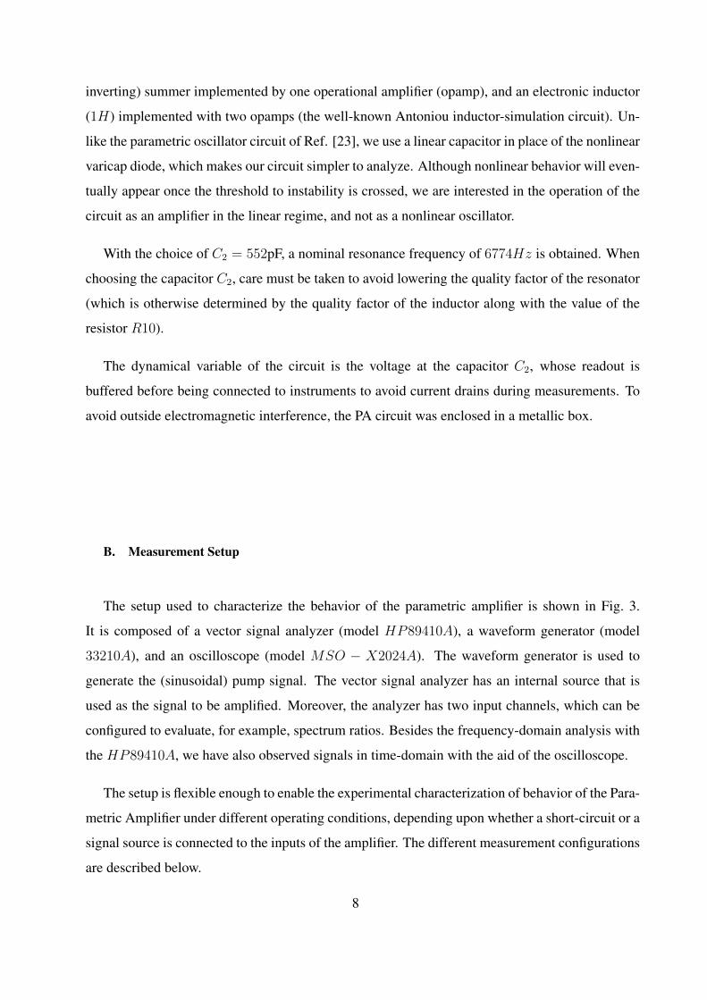
inverting) summer implemented by one operational amplifier (opamp), and an electronic inductor
(1H) implemented with two opamps (the well-known Antoniou inductor-simulation circuit). Un-
like the parametric oscillator circuit of Ref. [23], we use a linear capacitor in place of the nonlinear
varicap diode, which makes our circuit simpler to analyze. Although nonlinear behavior will even-
tually appear once the threshold to instability is crossed, we are interested in the operation of the
circuit as an amplifier in the linear regime, and not as a nonlinear oscillator.
With the choice of C2 = 552pF, a nominal resonance frequency of 6774Hz is obtained. When
choosing the capacitor C2, care must be taken to avoid lowering the quality factor of the resonator
(which is otherwise determined by the quality factor of the inductor along with the value of the
resistor R10).
The dynamical variable of the circuit is the voltage at the capacitor C2, whose readout is
buffered before being connected to instruments to avoid current drains during measurements. To
avoid outside electromagnetic interference, the PA circuit was enclosed in a metallic box.
B. Measurement Setup
The setup used to characterize the behavior of the parametric amplifier is shown in Fig. 3.
It is composed of a vector signal analyzer (model HP89410A), a waveform generator (model
33210A), and an oscilloscope (model MSO − X2024A). The waveform generator is used to
generate the (sinusoidal) pump signal. The vector signal analyzer has an internal source that is
used as the signal to be amplified. Moreover, the analyzer has two input channels, which can be
configured to evaluate, for example, spectrum ratios. Besides the frequency-domain analysis with
the HP89410A, we have also observed signals in time-domain with the aid of the oscilloscope.
The setup is flexible enough to enable the experimental characterization of behavior of the Para-
metric Amplifier under different operating conditions, depending upon whether a short-circuit or a
signal source is connected to the inputs of the amplifier. The different measurement configurations
are described below.
8
IV. NUMERICAL AND EXPERIMENTAL RESULTS
A. Harmonic oscillator resonant curve
To evaluate the response of the harmonic oscillator, for which Fp = 0 in Eq. (2), the pump input
port of the amplifier is short-circuited, while the signal input is fed with a signal source (please
refer to Fig. 3, connections b and d). We have measured the response (gain) of the harmonic
oscillator for a broad range of frequencies. The results are shown in Fig. 4. One can see that the
equivalent quality factor Q of the circuit was found to be about 65. This means that if we consider
the circuit of Fig. 1, the equivalent series resistance is about 619Ω. In addition to the 56Ω shown in
Fig. 2, there are additional losses attributed to the electronic inductor, since the quality factor of the
capacitor C2 was independently measured as about 124. The resonance frequency (f0 = ω0/(2π))
was found to be around 6400HZ , a value less than 6% lower than the nominal frequency.
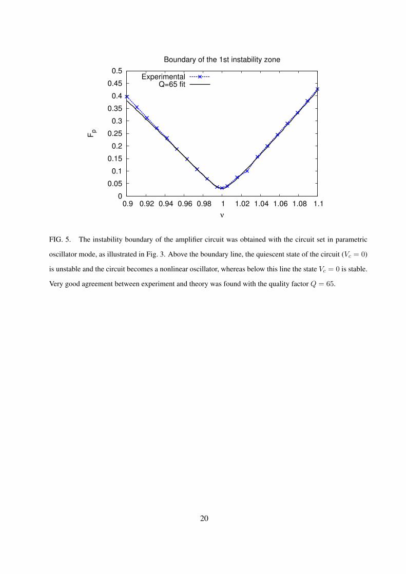
B. Instability boundary
After obtaining the resonance curve of the circuit in harmonic oscillator configuration, we have
evaluated the instability boundary of the circuit in parametric oscillator configuration. This con-
figuration is obtained by pumping the amplifier while short-circuiting its signal input. In Fig. 3,
this corresponds to connections a and c. For each value of pump frequency set, the pump am-
plitude was slowly increased from a very low initial value until an oscillation of more than 0.5V
in amplitude was observed at the output of the amplifier. When comparing the experimental data
against the numerical data from Eq. (2), we have found that the equivalent Q of the resonator is
about 65 (see Fig. 5), a value consistent with the one observed for the harmonic oscillator resonant
curve. Moreover, the instability line is centered on the same value of frequency found for the peak
of harmonic oscillator resonant curve (about 6400HZ), which represents half the value of pump
frequency for which the lowest pump amplitude is necessary for instability.
Hereafter the parameter values Q = γ−1 = 65 and ω0 ≈ 40212 rad/s will be used in fitting the
experimental data of parametric amplification against theoretical predictions.
9

C. Parametric amplification
Finally, we set the circuit in parametric amplification configuration, by inputing both pump and
signal, as described in Fig. 3 with connections a and d. In all the results presented below, the input
signal amplitude was limited to 2mV . Owing to the high gains which can be obtained, this value
has to be kept small enough to avoid saturation of the amplifier due to limitation of supply voltage
bias and intrinsic nonlinearities of the active components of the circuit.
In Fig. 6, we show a time series obtained from the circuit set with pump amplitude Vp = 3V ,
pump frequency 1.8f0 and input signal frequency fs = 0.95f0, along with the envelope predicted
by the Eq. (10) with Fp = 0.3.
In Fig. 7, we show a time series obtained from the circuit set with pump amplitude Vp = 0.29V ,
pump frequency 2f0 and input signal frequency fs = 0.99f0, along with the envelope predicted
by the Eq. (10) with Fp = 0.029. The best agreement between the experimental time series and
the theoretical envelope is obtained under this condition (degenerate-mode amplification). This
occurs because the accuracy of the perturbative methods used (averaging and harmonic balance)
is higher the smaller the parameter Fp is.
In Fig. 8, we show a time series obtained from the circuit set with pump amplitude Vp = 4V ,
pump frequency 2.2f0 and input signal frequency fs = 1.05f0, along with the envelope predicted
by the Eq. (10) with Fp = 0.4.
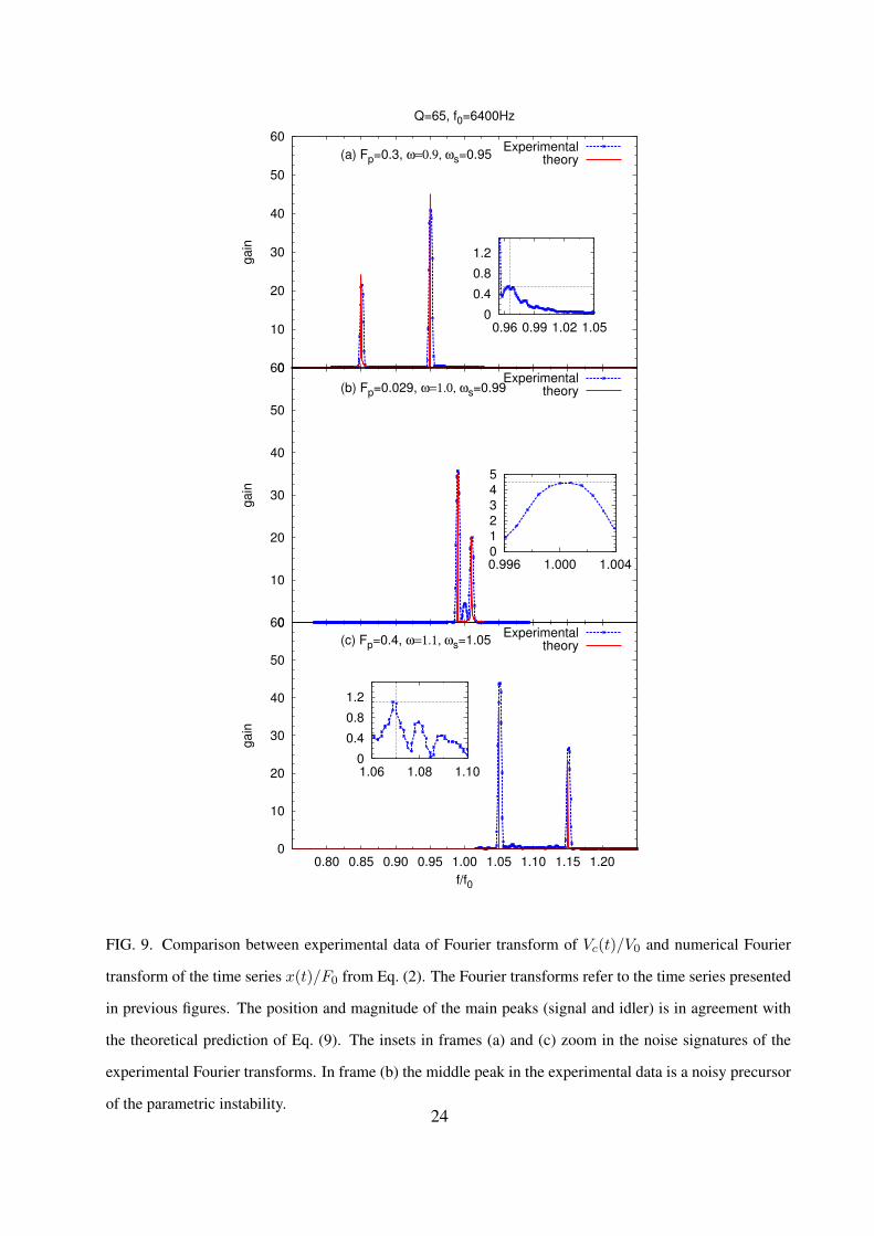
In Fig. 9, we show the signal spectrum measured at the output of the amplifier with the aid
of the signal analyzer (please refer to Fig. 3). The experimental conditions correspond respec-
tively to those associated with the time series presented in Figs. 6, 7, and 8. The signal analyzer
computes the spectrum concurrently to the acquisition of the waveforms by the Oscilloscope. The
experimental results are compared against the numerical Fourier transforms of the time series x(t)
obtained from numerical integration of Eq. (2). The position and magnitude of the main peaks
(signal and idler) is in agreement with the theoretical predictions of Eq. (9). In frame (b), the
middle peak in the experimental data is a noisy precursor of the parametric instability, whereas
in frames (a) and (c) one hardly notices any effects of noise. To help visualize these effects, the
insets in frames (a) and (c) show details of noisy precursors in the experimental data. Further be-
low we will explain why these precursors are more relevant in the degenerate-mode amplification
of frame (b), than in cases (a) and (c). In all cases, though, the response of the PA to noise is
more pronounced when the amplifier is tuned to the vicinity of the transition line [20–22]. Hence,
10
the closer one gets to the transition line, the higher the noisy precursor lines in the spectrum will
be. A detailed analysis of the noise spectrum is made in the next subsection. The noisy precursor
effect is in qualitative agreement with the observations of Jeffries and Wiesenfeld on the effect of
broadband noise on the power spectrum of coherent signals, which was first investigated (theoreti-
cally and experimentally) near period-doubling and Hopf bifurcations in a periodically driven p-n
junction [18, 19] and in the context of parametric amplification in Josephson junctions [24].
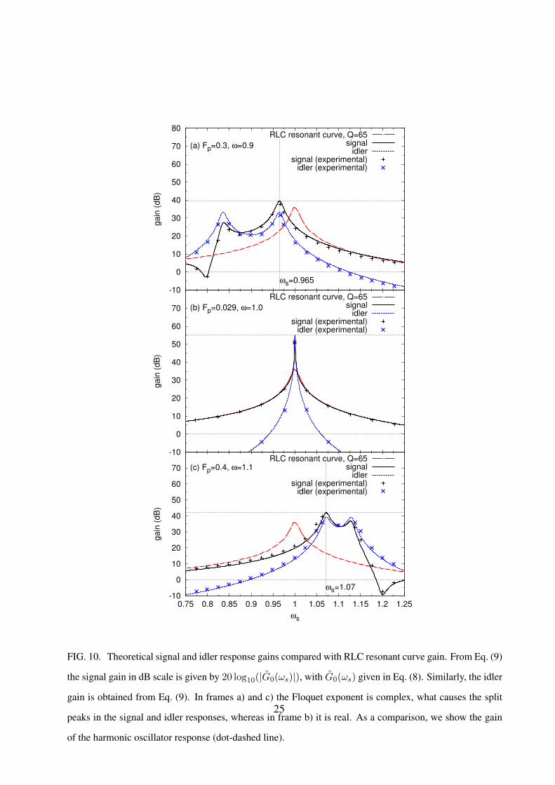
In Fig. 10 one can see the signal and idler responses of the PA as a function of frequency.
Again, one can see that there is a much broader bandwidth of gain in quasi-degenerate mode of
amplification, such as in frames (a) and (c), than in degenerate-mode amplification, frame (b).
Moreover, the bandwidth of gain, the peak positions, and the gain×bandwidth product can be
tuned as well, unlike in the degenerate-mode amplification.
D. Noise spectral density
The spectra of the signal responses can be used to predict where the lines due to noise will turn
up in the Fourier transform of the time series x(t), as shown in Fig. 9. Since there is always a
small amount of added noise of very broad bandwidth, which comes along with the input ac signal
or is intrinsic to the circuit, there will be noise components everywhere in the spectra of Fig. 10.
Hence, as our system is linear, the spectral components of noise will be amplified in the same
way as the input ac signals are amplified. The strongest case is seen at the peak of degenerate-
mode parametric amplification, when ωs = 1, where the noise will be amplified roughly by 55dB.
The corresponding noise line can be seen in Fig. 9(b). The noise lines in quasi-degenerate-mode
parametric amplification are much smaller, since the the peaks in frames 10(a) and (c) have gains
of only roughly 39dB and 42dB, respectively. Nonetheless, if one looks in the insets of frames
(a) and (c) of Fig. 9, one can see elevations in the noise level exactly at the peaks of the signal
response of Fig. 10. The horizontal and vertical dashed lines at the signal peaks of Fig. 10 are
reproduced in the insets of Fig. 9 for clarity. One can then compare the magnitudes of the noise
line peaks of Fig. 9. The difference in gain at noise line peaks between frame 9(b) and (a) is
20 log10(4.5/0.55) = 18.2dB, whereas between frame (b) and (c) is 20 log10(4.5/1.1) = 12.2dB.
On the other hand, the predicted differences in noise peaks based on theory for the signal gain
shown in Fig. 10 is 16dB and 13dB, respectively. These results show that our experimental results
are consistent with the predictions of our proposed linear theory to within an error of under 2.5dB.
11

We note that the same noise signatures appear in the spectrum when there is no input ac signal,
confirming that the noise precursors are a consequence of linear response and a consequence of
the signal gain spectra of the PA, such as the ones presented in Fig. 10.
In Fig. 11 we show the noise spectral density for our circuit setup in harmonic oscillator mode.
Here we fit the data with a noise intensity of D = 3.08 × 10⁻⁸V2/Hz. The source of this noise
is intrinsic to the circuit. Here we showed the exact theoretical result for the NSD of a harmonic
oscillator process given by S0x alongside the approximate result Sx from Eq. (18). In our units
Sx has dimensions of V 2, since the time is adimensional. In order to set it in proper units, Sx is
divided by ω0. Both theoretical predictions yield nearly the same spectrum and account well for
the experimental data. On the other hand, the NSD from Eq. (13) of Ref. [18] gives a result that
is 6dB higher than the measured noise. Apart from this, their result can be rescaled to be exactly
our result from Eq. (18) if one divides their prediction by 4. Here we have a way of measuring
the noise level when there is no pumping, whereas in their model, there is no quiescent solution
without noise. They developed a perturbative solution due to noise around a limit cycle (an isolated
periodic solution) and did not calibrate their solution in the zero pumping limit.
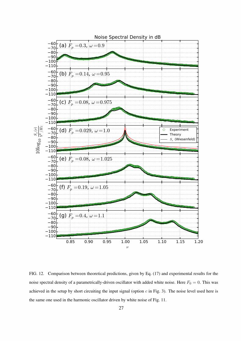
In Fig. 12 one can see the comparison between theoretical predictions, given by Eq. (17) or
by Jeffries-Wiesenfeld model, and experimental results for the NSD of a parametrically-driven
oscillator with added white noise. Here, the noise level used to fit the data was the same one of
the harmonic oscillator configuration. In frames (a-c) and (e-g) the Floquet exponents are still
complex, as can be seen in the gap between the noise peaks. These peaks are located symmetri-
cally with respect to ω and the distance between them is twice the imaginary part of the Floquet
exponents. In frame (d) the Floquet exponents are real and, hence, there is no split peak in the
noise spectrum. The discrepancy of theory and experiment at the peak of the NSD is certainly
due to nonlinear effects not accounted for by our linear model. Again here the Jeffries-Wiesenfeld
model is off with a level of noise higher by slightly over 6dB. Note also that the absence of sharp
peaks in the spectrum is because we have a quiescent solution and not a periodic orbit solution
when there is no noise.
V. CONCLUSION
Here we obtained experimental results on gain and bandwidth of classical parametric ampli-
fication that are quantitatively well approximated by a theory based on averaging techniques and
12

on Green’s function theory. Although one can reach extremely high values of gain in degenerate
mode parametric amplification, the corresponding bandwidth is very narrow. This is sometimes
an undesirable characteristics, since it makes tuning to the signal a difficult task. We have found
that the bandwidth of the parametric amplifier can be increased if we set the amplifier in quasi-
degenerate-mode amplification, i.e. with detuning (Ω 6= 0). This comes at the expense of the high
gain obtained in degenerate-mode amplification. Guided by the model developed here, the opti-
mal amount of gain and bandwidth could be found by carefully tuning the pump frequency and the
pump amplitude. Moreover, the bandwidth of gain, the peak positions, and the gain×bandwidth
product can be tuned as well, unlike in the degenerate-mode amplification.
Furthermore, we presented a theory for obtaining an approximate analytical expression for the
NSD of the parametric oscillator with added noise that accounts for the noisy precursors of insta-
bility in the PA. With the information of the signal and idler gain spectra and the input noise level,
one could, in principle, determine how the noise features will be manifested in the power spectrum
of the output signal of the PA. Although Wiesenfeld et al. [18, 19] developed a general compre-
hensive model for accounting for the noisy precursors of bifurcations of codimension-1 based on
Floquet theory, the model we propose is simpler to apply and has all the theoretical expressions
necessary to compare with experimental results. It does not depend on generic unspecified Floquet
exponents. It is worthy to mention that the present model describes the simplest nontrivial system
to which the generic theory of Wiesenfeld could be applied to, but which was actually overlooked
in the literature so far to the authors knowledge. Furthermore, we have results for the noise spectral
density that take into account the presence of two Floquet multipliers, and not just one as described
in Ref. [19]. The existence of two complex Floquet multipliers is characterized by the appearance
of two noise peaks in the NSD spectrum, which can be seen in several of our results. This is
especially relevant in high Q parametric oscillators, where the stable parameter region in which
the Floquet amplifiers are real decreases with increasing Q. Hence, it becomes harder to tune into
this region, specially, when there is detuning in the pump frequency with respect to the resonance
frequency, so one has to account for the contribution from both Floquet exponents. Also, due to
this, the noisy precursors spectral curves are not properly Lorenzian anymore.
The predicted gain curves proposed here can be used to determine signal and idler gains, the
output noise spectral density, and the figure of noise of the PA (ratio of output and input signal-
to-noise ratios of the PA). Furthermore, our PA circuit can be used as a simple and inexpensive
experimental platform to test recent theoretical predictions [20–22] on thermal noise squeezing.
13

Finally, the close proximity of the theoretical predictions and the experimental results obtained
here indicates that one could design electronic devices based on PAs that could achieve extremely
high gains, have very little noise, and be tunable. Future experimental and theoretical work on the
PAs will be performed in analyzing the effects of nonlinearity on the dynamic range of amplifica-
tion and the phenomenon of noise squeezing.
Appendix: Idler response calculations
The idler response is given by∫ t
−∞dt′ Gp(t, t
′) cos(ωst′ + φ0) =
∫ ∞0
dτ Gp(t, t− τ) cos(ωs(t− τ) + φ0)
= − β
ωκ
∫ ∞0
dτ e−γτ/2 sinh(κ τ) cos(ω(2t− τ)) cos(ωs(t− τ) + φ0)
= − β
2ωκ
∫ ∞0
dτ e−γτ/2 sinh(κ τ) [cos ((ω + ωs)(t− τ) + ωt+ φ0) + cos ((ω − ωs)(t− τ) + ωt− φ0)]
= − β
2ωκReeiωt
∫ ∞0
dτ e−γτ/2 sinh(κ τ)[ei[(ω+ωs)(t−τ)+φ0] + ei[(ω−ωs)(t−τ)−φ0]
]= − β
2ωRe
ei[(2ω+ωs)t+φ0]
[γ/2− κ+ i(ω + ωs)][γ/2 + κ+ i(ω + ωs)]
+ei[(2ω−ωs)t−φ0]
[γ/2− κ+ i(ω − ωs)][γ/2 + κ+ i(ω − ωs)]
, (A.1)
where we used the following result∫ ∞0
dτ e−[γ/2+i(ω±ωs)]τ sinh(κ τ) =1
2
[1
γ/2− κ+ i(ω ± ωs)− 1
γ/2 + κ+ i(ω ± ωs)
]=
κ
[γ/2− κ+ i(ω ± ωs)][γ/2 + κ+ i(ω ± ωs)]. (A.2)
Appendix: Noise response
We have to solve∫ ∞t′
dt eiνtGp(t, t′) ≈ − β
κωeγt
′/2
∫ ∞t′
dt eiνte−γt/2 sinh(κ (t− t′)) cos(ω(t+ t′)),
∫ ∞t′
dt e(−γ/2+iν)t sinh(κ (t− t′)) cos(ω(t+ t′)) =eiωt
′
2
∫ ∞t′
dt e[−γ/2+i(ν+ω)]t sinh(κ (t− t′))
+e−iωt
′
2
∫ ∞t′
dt e[−γ/2+i(ν−ω)]t sinh(κ (t− t′))
(A.1)
14
∫ ∞t′
dt e[−γ/2+i(ω+ν)]t sinh(κ (t− t′)) = I1 + I2,
where
I1 =e−κt
′
2
∫ ∞t′
dt e[−γ/2+i(ν+ω)]teκ t =e[−γ/2+i(ν+ω)]t′
γ − 2κ− 2i(ν + ω)
I2 = −eκt′
2
∫ ∞t′
dt e[−γ/2+i(ν+ω)]te−κ t = − e[−γ/2+i(ν+ω)]t′
γ + 2κ− 2i(ν + ω)
I1 + I2 = e[−γ/2+i(ω+ν)]t′[
1
γ − 2κ− 2i(ω + ν)− 1
γ + 2κ− 2i(ω + ν)
]=
4κe[−γ/2+i(ω+ν)]t′
[γ − 2κ− 2i(ω + ν)][γ + 2κ− 2i(ω + ν)](A.2)∫ ∞
t′dt e[−γ/2+i(ν−ω)]t sinh(κ (t− t′)) = K1 +K2,
where
K1 =e−κt
′
2
∫ ∞t′
dt e[−γ/2+i(ν−ω)]teκ t =e[−γ/2+i(ν−ω)]t′
γ − 2κ− 2i(ν − ω)
K2 = −eκt′
2
∫ ∞t′
dt e[−γ/2+i(ν−ω)]te−κ t = − e[−γ/2+i(ν−ω)]t′
γ + 2κ− 2i(ν − ω)
∫ ∞t′
dt eiνtGp(t, t′) ≈ − β
κωeγt
′/2[(I1 + I2)eiωt
′+ (K1 +K2)e−iωt
′]/2
≈ − β
2ω
[ei(ν+2ω)t′
[γ/2− κ− i(ν + ω)][γ/2 + κ− i(ν + ω)]
+ei(ν−2ω)t′
[γ/2− κ− i(ν − ω)][γ/2 + κ− i(ν − ω)]
]
∫ ∞−∞
dt′r(t′)
∫ ∞t′
dt eiνtGp(t, t′) ≈ − β
2ω
[r(ν + 2ω)
[γ/2− κ− i(ν + ω)][γ/2 + κ− i(ν + ω)]
+r(ν − 2ω)
[γ/2− κ− i(ν − ω)][γ/2 + κ− i(ν − ω)]
].
[1] M. Faraday, Philos. Trans. R. Soc. London 121, 319 (1831).
[2] L. Ruby, Am. J. Phys. 64, 39 (1996).
[3] W. Mumford, Proceedings of the IRE 48, 848 (1960).
15

[4] W. Paul, Rev. of Mod. Phys. 62, 531 (1990).
[5] M. G. Raizen, J. M. Gilligan, J. C. Bergquist, W. M. Itano, and D. J. Wineland, Phys. Rev. A 45, 6493
(1992).
[6] M. Drewsen, C. Brodersen, L. Hornekær, J. S. Hangst, and J. P. Schifffer, Phys. Rev. Lett. 81, 2878
(1998).
[7] D. Kielpinski, C. Monroe, and D. J. Wineland, Nature 417, 709 (2002).
[8] W. M. Dougherty, K. J. Bruland, J. L. Garbini, and J. Sidles, Meas. Sci. and Technol. 7, 1733 (1996).
[9] M. Moreno-Moreno, A. Raman, J. Gomez-Herrero, and R. Reifenberger, Appl. Phys. Lett. 88, 193108
(2006).
[10] M. V. Requa and K. L. Turner, Appl. Phys. Lett. 88, 263508 (2006).
[11] O. Thomas, F. Mathieu, W. Mansfield, C. Huang, S. Trolier-McKinstry, and L. Nicu, Applied Physics
Letters 102, 163504 (2013).
[12] K. L. Turner, S. A. Miller, P. G. Hartwell, N. C. MacDonald, S. H. Strogatz, and S. G. Adams, Nature
396, 149 (1998).
[13] B. H. Eom, P. K. Day, H. G. LeDuc, and J. Zmuidzinas, Nature Phys. 8, 623 (2012).
[14] A. Szorkovszky, A. C. Doherty, G. I. Harris, and W. P. Bowen, Phys. Rev. Lett. 107, 213603 (2011).
[15] M. Castellanos-Beltran, K. Irwin, G. Hilton, L. Vale, and K. Lehnert, Nature Physics 4, 929 (2008).
[16] G. Binnig, C. F. Quate, and C. Gerber, Phys. Rev. Lett 56, 930 (1986).
[17] D. Rugar and P. Grutter, Phys. Rev. Lett. 67, 699 (1991).
[18] C. Jeffries and K. Wiesenfeld, Phys. Rev. A 31, 1077 (1985).
[19] K. Wiesenfeld, J. of Stat. Phys. 38, 1071 (1985).
[20] A. A. Batista, Phys. Rev. E 86, 051107 (2012).
[21] A. A. Batista, J. of Stat. Mech. (Theory and Experiment) 2011, P02007 (2011).
[22] A. A. Batista and R. S. N. Moreira, Phys. Rev. E 84, 061121 (2011).
[23] R. Berthet, A. Petrosyan and B. Roman, Am. J. Phys. 70, 744 (2002).
[24] P. Bryant, K. Wiesenfeld, and B. McNamara, J. Appl. Phys. 62, 2898 (1987).
16

R
L
C Vpcos (4πft)
ΣxVc
V0cos(2πfst+φ0)
FIG. 1. Schematic block diagram of the proposed analog electronic implementation of the parametric
amplifier. The box on the left represents a multiplier with gain A and the box on the right is a non-inverting
summer.
R1
1kΩ
R2
1kΩ
R3
1kΩ
R4
1kΩ
C1
1µF
C2552pF
R1056Ω
U3B
TL084ACD
5611
4
7
U3A
TL084ACD
3 2114
1
U1
AD633JN
X1
X2
Y1
Y2 VS-
Z
W
VS+
R7
1kΩ
R8
1kΩ
R9
1kΩ
U2D
TL084ACD
12
13 11
4
14
Multiplier
Electronic Inductor
Summer
Input signalPump signalOutput
FIG. 2. Electronic circuit implementing the parametric amplifier. The 1H electronic inductor is im-
plemented with the aid of operational amplifiers. The IC AD633 represents the multiplier,with a gain of
10V −1. For simplicity, the output buffer and the power supplies are not shown.
17

Waveform Generator
Signal
Pump
Output
Channel 1
Channel 2Source
Frequency-domain
measurements
Time-domain
measurementsSHORT-
CIRCUIT
OR
SHORT-
CIRCUIT
OR
Parametric
Amplifier
Vector Signal Analyzer with Internal Source
Oscilloscope
a b
c d
FIG. 3. Setup used to characterize the behavior of the parametric amplifier, allowing different operating
conditions. With options b and d, the PA behaves as a driven harmonic oscillator. With options a and c, the
PA behaves as a parametric oscillator. With options a and d, the PA behaves as a parametric amplifier if the
pump is kept below the instability threshold.
18

0
10
20
30
40
50
60
70
80
5600 5800 6000 6200 6400 6600 6800 7000 7200
X/F
0
fs (Hz)
experimentfit with Q=65
FIG. 4. Harmonic oscillator (pump off) resonant curve, obtained using connections b and d in Fig. 3. Here
we fit the experimental resonant curve with the theoretic prediction and find a Q of approximately 65 and a
resonant frequency of f0 = 6400Hz.
19
0
0.05
0.1
0.15
0.2
0.25
0.3
0.35
0.4
0.45
0.5
0.9 0.92 0.94 0.96 0.98 1 1.02 1.04 1.06 1.08 1.1
Fp
ν
Boundary of the 1st instability zone
ExperimentalQ=65 fit
FIG. 5. The instability boundary of the amplifier circuit was obtained with the circuit set in parametric
oscillator mode, as illustrated in Fig. 3. Above the boundary line, the quiescent state of the circuit (Vc = 0)
is unstable and the circuit becomes a nonlinear oscillator, whereas below this line the state Vc = 0 is stable.
Very good agreement between experiment and theory was found with the quality factor Q = 65.
20

-100
-50
0
50
100
-0.0045 -0.003 -0.0015 0 0.0015 0.003
Vc(t
)/V
0
t (sec)
Q=65,ω=0.9, ωs=0.95, Fp=0.3
experimenttheory
FIG. 6. Comparison between a time series from experimental data of Vc(t) and corresponding envelope
obtained from theory in Eq. (10). The amplification here is set in quasi-degenerate mode with all parameters
indicated in the figure.
21

-100
-50
0
50
100
-0.02 -0.015 -0.01 -0.005 0 0.005 0.01 0.015 0.02
Vc(t
)/V
0
t (sec)
Q=65,ω=1.0, ωs=0.99, Fp=0.029
experimenttheory
FIG. 7. Comparison between time series of experimental data of Vc(t) and envelope obtained from theory
in Eq. (10). The amplification here is set in degenerate mode with a small detuning between half the pump
frequency, ω = 1, and the input signal frequency, ωs = 0.99.
22

-100
-80
-60
-40
-20
0
20
40
60
80
100
0 0.0015 0.003 0.0045 0.006 0.0075 0.009
Vc(t
)/V
0
t (sec)
Q=65,ω=1.1, ωs=1.05, Fp=0.4
experimenttheory
FIG. 8. Comparison between a time series from experimental data of Vc(t) and envelope obtained from
theory in Eq. (10). The amplification here is set in quasi-degenerate mode. All parameters are indicated in
the figure.
23
0
10
20
30
40
50
60
gain
Q=65, f0=6400Hz
(a) Fp=0.3, ω=0.9, ωs=0.95Experimental
theory
0
0.4
0.8
1.2
0.96 0.99 1.02 1.05
0
10
20
30
40
50
60
gain
(b) Fp=0.029, ω=1.0, ωs=0.99Experimental
theory
0 1 2 3 4 5
0.996 1.000 1.004
0
10
20
30
40
50
60
0.80 0.85 0.90 0.95 1.00 1.05 1.10 1.15 1.20
gain
f/f0
(c) Fp=0.4, ω=1.1, ωs=1.05Experimental
theory
0
0.4
0.8
1.2
1.06 1.08 1.10
FIG. 9. Comparison between experimental data of Fourier transform of Vc(t)/V0 and numerical Fourier
transform of the time series x(t)/F0 from Eq. (2). The Fourier transforms refer to the time series presented
in previous figures. The position and magnitude of the main peaks (signal and idler) is in agreement with
the theoretical prediction of Eq. (9). The insets in frames (a) and (c) zoom in the noise signatures of the
experimental Fourier transforms. In frame (b) the middle peak in the experimental data is a noisy precursor
of the parametric instability.24
-10
0
10
20
30
40
50
60
70
80
gain
(dB
)
(a) Fp=0.3, ω=0.9
ωs=0.965
RLC resonant curve, Q=65signal
idlersignal (experimental)
idler (experimental)
-10
0
10
20
30
40
50
60
70
gain
(dB
)
(b) Fp=0.029, ω=1.0
RLC resonant curve, Q=65signal
idlersignal (experimental)
idler (experimental)
-10
0
10
20
30
40
50
60
70
0.75 0.8 0.85 0.9 0.95 1 1.05 1.1 1.15 1.2 1.25
gain
(dB
)
ωs
(c) Fp=0.4, ω=1.1
ωs=1.07
RLC resonant curve, Q=65signal
idlersignal (experimental)
idler (experimental)
FIG. 10. Theoretical signal and idler response gains compared with RLC resonant curve gain. From Eq. (9)
the signal gain in dB scale is given by 20 log10(|G0(ωs)|), with G0(ωs) given in Eq. (8). Similarly, the idler
gain is obtained from Eq. (9). In frames a) and c) the Floquet exponent is complex, what causes the split
peaks in the signal and idler responses, whereas in frame b) it is real. As a comparison, we show the gain
of the harmonic oscillator response (dot-dashed line).
25

0.85 0.90 0.95 1.00 1.05 1.10 1.15 1.20ν
115
110
105
100
95
90
85
80
7510l
og 1
0Sx(ν
)
V2/Hz
Harmonic Oscillator Noise Spectral Density
ExperimentSx with Fp =0, ω=1
S 0x
Sx (Wiesenfeld)
FIG. 11. Comparison between theoretical predictions and experimental results for the noise spectral density
of a harmonic oscillator. Here F0 = 0. The measuring apparatus depicted in Fig. 3 was setup such that the
Signal and the Pump ports were short-circuited (options b and c). The results for Sx are given by Eq. (17)
without parametric pumping and at resonance, whereas S0x is the exact harmonic oscillator spectral density.
26
110100
90807060 (a) Fp =0.3, ω=0.9
Noise Spectral Density in dB
110100
90807060 (b) Fp =0.14, ω=0.95
ν
110100
90807060 (c) Fp =0.08, ω=0.975
110100
90807060
10lo
g 10Sx(ν
)
V2/Hz
(d) Fp =0.029, ω=1.0 ExperimentTheorySx (Wiesenfeld)
110100
90807060 (e) Fp =0.08, ω=1.025
110100
90807060 (f) Fp =0.19, ω=1.05
0.85 0.90 0.95 1.00 1.05 1.10 1.15 1.20ν
110100
90807060 (g) Fp =0.4, ω=1.1
FIG. 12. Comparison between theoretical predictions, given by Eq. (17) and experimental results for the
noise spectral density of a parametrically-driven oscillator with added white noise. Here F0 = 0. This was
achieved in the setup by short circuiting the input signal (option c in Fig. 3). The noise level used here is
the same one used in the harmonic oscillator driven by white noise of Fig. 11.
27


