
Abdul Abiad (team lead), Aseel Almansour, Davide Furceri, Carlos Mulas-Granados, and Petia Topalova
with contributions from the Economic Modeling and Development Macroeconomic Division , and
with support from Angela Espiritu, Sinem Kilic Celik, and Olivia Ma
Is it Time for an Infrastructure Push? The Macroeconomic Effects of Public Investment

Outline of Presentation
• Motivation and Summary of Main Findings
• The Economic of Infrastructure
• Public and Infrastructure Capital and Investment: Where Do We Stand?
• The Macroeconomic Effects of Public Investment
• Policy Implications

Motivation and Main Findings

Motivation- Why look at public investment now?
• In AEs, there is still a lot of slack, compounded by worries over secular stagnation
• In many EMDEs, infrastructure bottlenecks are contributing to slower growth
• Across all economies, there are concerns about long-run potential, with insufficient public/infrastructure investment being one of the reasons for concern
• Given the current environment of low borrowing costs, might this be a good time to increase public investment?

Summary of main findings: the time is right for an infrastructure push
• The stock of public capital, a proxy for infrastructure, has declined significantly as a share of output over the past three decades across the world – In emerging market and developing economies, gaps in the quantity of infrastructure per
capita are glaring
– In some advanced economies the quality of the existing infrastructure stock is deteriorating
• Higher public infrastructure investment boosts output in the short and long term
• The effects are stronger during periods of economic slack and monetary accommodation, and when investment efficiency is high
• Debt-financed public investment tends to have large output effects without increasing the debt-to-GDP ratio

The Economic of Infrastructure
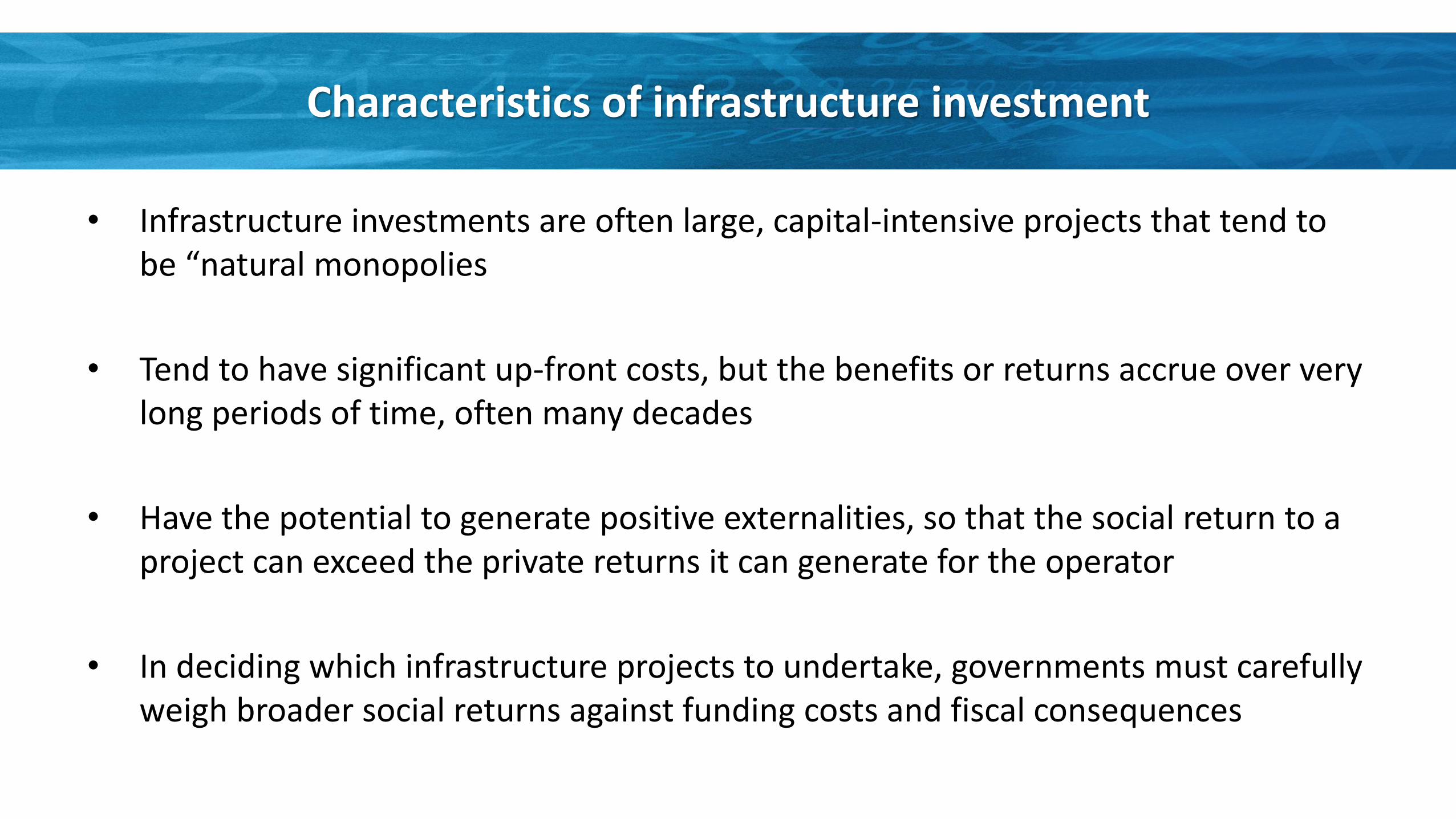
Characteristics of infrastructure investment
• Infrastructure investments are often large, capital-intensive projects that tend to be “natural monopolies
• Tend to have significant up-front costs, but the benefits or returns accrue over very long periods of time, often many decades
• Have the potential to generate positive externalities, so that the social return to a project can exceed the private returns it can generate for the operator
• In deciding which infrastructure projects to undertake, governments must carefully weigh broader social returns against funding costs and fiscal consequences

The macroeconomic effect of infrastructure investment: a conceptual framework
• Infrastructure investments increases output in the short-term by boosting aggregate demand – the size of the effect depends on the state of the economy
• Infrastructure investments increases output in the long-term by boosting aggregate supply – the size of the effect depends on the efficiency of investment
• If short-term multipliers, public investment efficiency, and the elasticity of output to public capital are sufficiently high, an increase in public investment can be “self-financing” in that it leads to a reduction in the debt-to-GDP ratio

Public and Infrastructure Capital and Investment: Where Do We Stand?
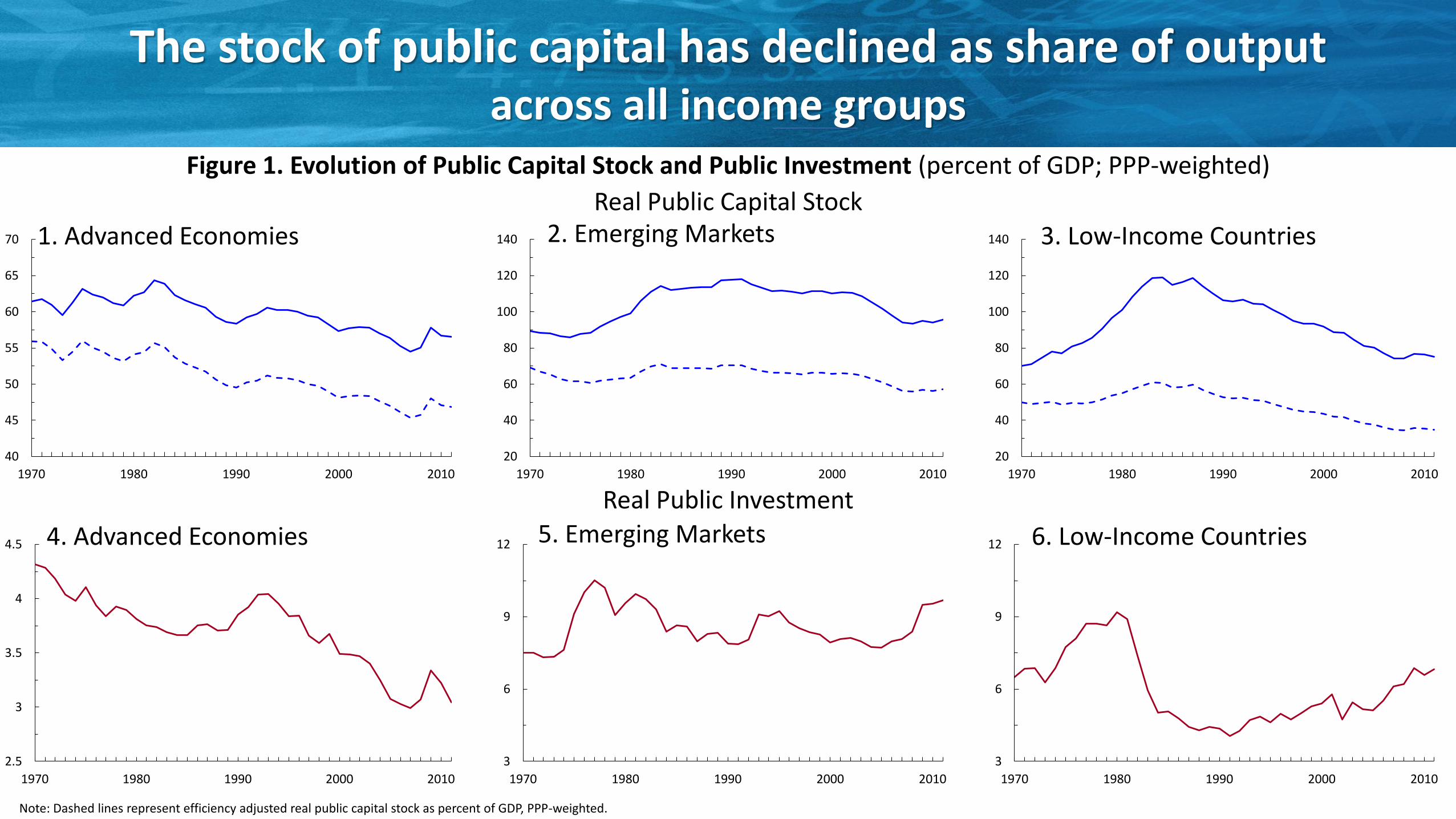
The stock of public capital has declined as share of output across all income groups
40
45
50
55
60
65
70
1970 1980 1990 2000 2010
20
40
60
80
100
120
140
1970 1980 1990 2000 2010
20
40
60
80
100
120
140
1970 1980 1990 2000 2010
Figure 1. Evolution of Public Capital Stock and Public Investment (percent of GDP; PPP-weighted)
Real Public Investment
1. Advanced Economies
2.5
3
3.5
4
4.5
1970 1980 1990 2000 2010
3
6
9
12
1970 1980 1990 2000 2010
3
6
9
12
1970 1980 1990 2000 2010
4. Advanced Economies
2. Emerging Markets 3. Low-Income Countries
5. Emerging Markets 6. Low-Income Countries
Note: Dashed lines represent efficiency adjusted real public capital stock as percent of GDP, PPP-weighted.
Real Public Capital Stock

In EMDEs infrastructure gaps are glaring
0 50
100 150 200 250 300 350 400
North America Adv. Asia Adv. Europe CIS Em. and Dev. Europe LAC MENAP Em. and Dev. Asia SSA
0
0.5
1
1.5
2
2.5
North America Adv. Europe Adv. Asia Em. and Dev. Europe CIS LAC Em. and Dev. Asia MENAP SSA
0
50
100
150
200
250
Adv. Europe CIS Adv. Asia North America Em. and Dev. Europe LAC MENAP Em. and Dev. Asia SSA
1. Electricity Generating Capacity (kilowatts per 100 people), 2010
2. Roads (kilometers per 100 people), 2010
3. Phone Lines (land and cell phone lines per 100 people), 2010
correlation
Figure 2. Physical Measures of Infrastructure (percent of GDP; PPP-weighted)

Figure 3. Quality of Infrastructure in G7 Economies (Scale, 1–7; higher score indicates better infrastructure)
2006 2007 2008 2009 2010 2011 2012
0
1
2
3
4
5
6
7
Germany France United States Japan Canada United Kingdom Italy
In some AEs the quality of infrastructure is deteriorating
1. Overall Quality
0
1
2
3
4
5
6
7
Germany France United States Japan Canada United Kingdom Italy
2. Road Quality

Macroeconomic Effects of Public Investment in AEs: Empirical Evidence
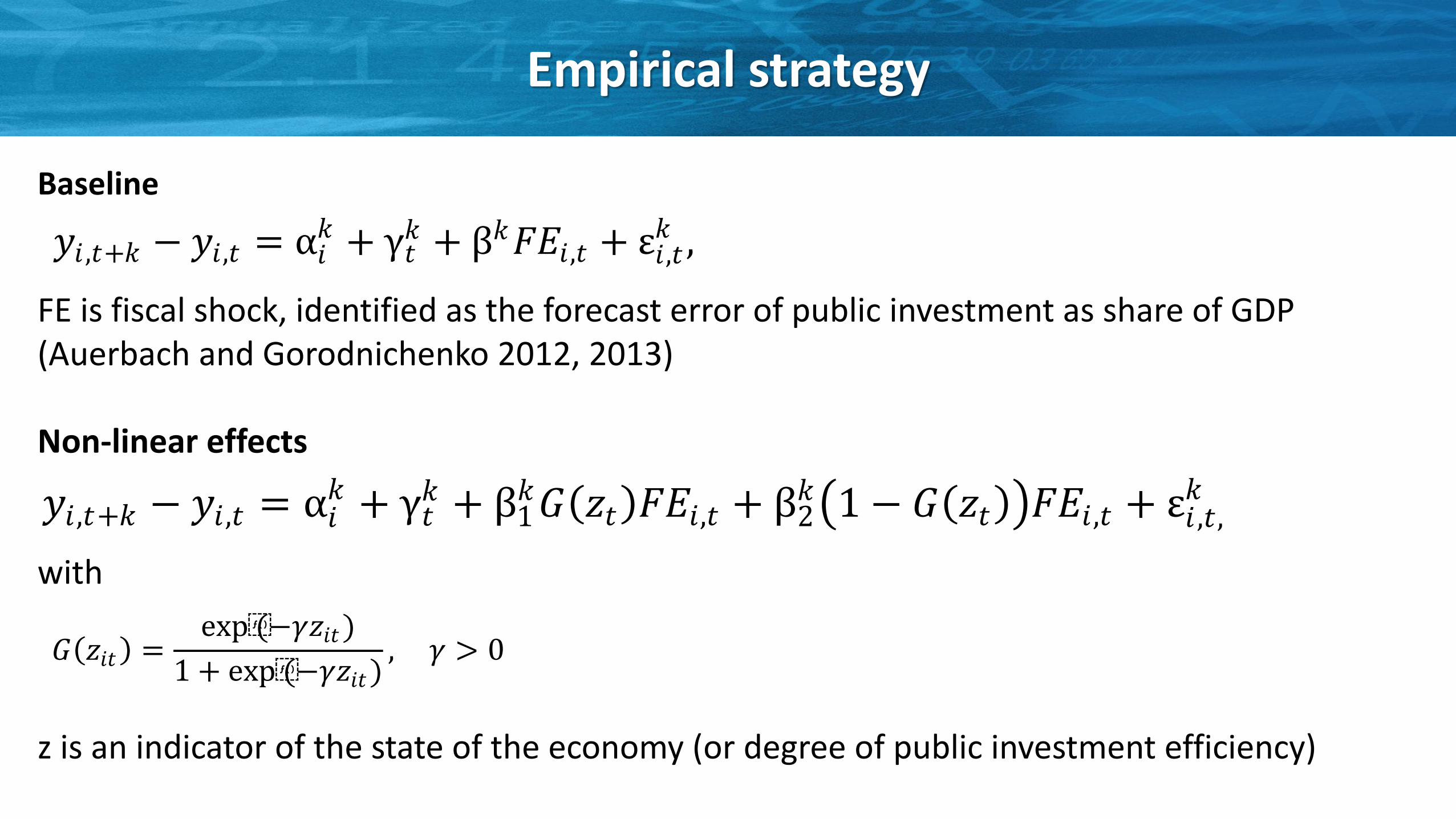
Baseline FE is fiscal shock, identified as the forecast error of public investment as share of GDP (Auerbach and Gorodnichenko 2012, 2013) Non-linear effects with z is an indicator of the state of the economy (or degree of public investment efficiency)
Empirical strategy
𝐺 𝑧𝑖𝑡 =exp(−𝛾𝑧𝑖𝑡)
1 + exp(−𝛾𝑧𝑖𝑡), 𝛾 > 0
𝑦𝑖 ,𝑡+𝑘 − 𝑦𝑖,𝑡 = α𝑖𝑘 + γ𝑡
𝑘 + β𝑘𝐹𝐸𝑖,𝑡 + ε𝑖,𝑡𝑘 ,
𝑦𝑖,𝑡+𝑘 − 𝑦𝑖,𝑡 = α𝑖𝑘 + γ𝑡
𝑘 + β1𝑘𝐺 𝑧𝑡 𝐹𝐸𝑖,𝑡 + β2
𝑘 1 − 𝐺 𝑧𝑡 𝐹𝐸𝑖,𝑡 + ε𝑖 ,𝑡,𝑘
Baseline results
0
1
2
3
–1 0 1 2 3 4
-10
-8
-6
-4
-2
0
2
–1 0 1 2 3 4
-1
-0.5
0
0.5
1
–1 0 1 2 3 4
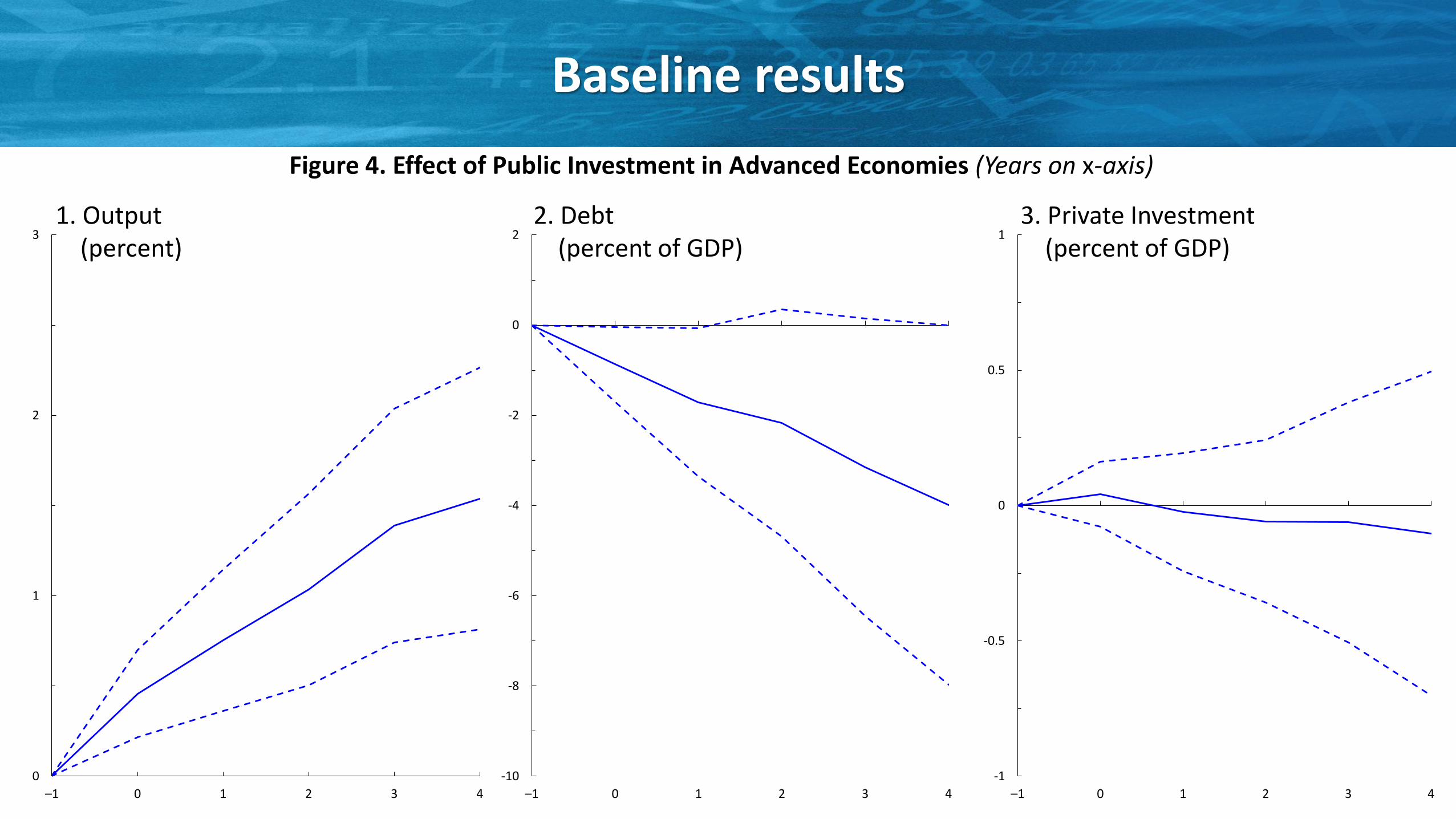
Figure 4. Effect of Public Investment in Advanced Economies (Years on x-axis)
1. Output (percent)
2. Debt (percent of GDP)
3. Private Investment (percent of GDP)
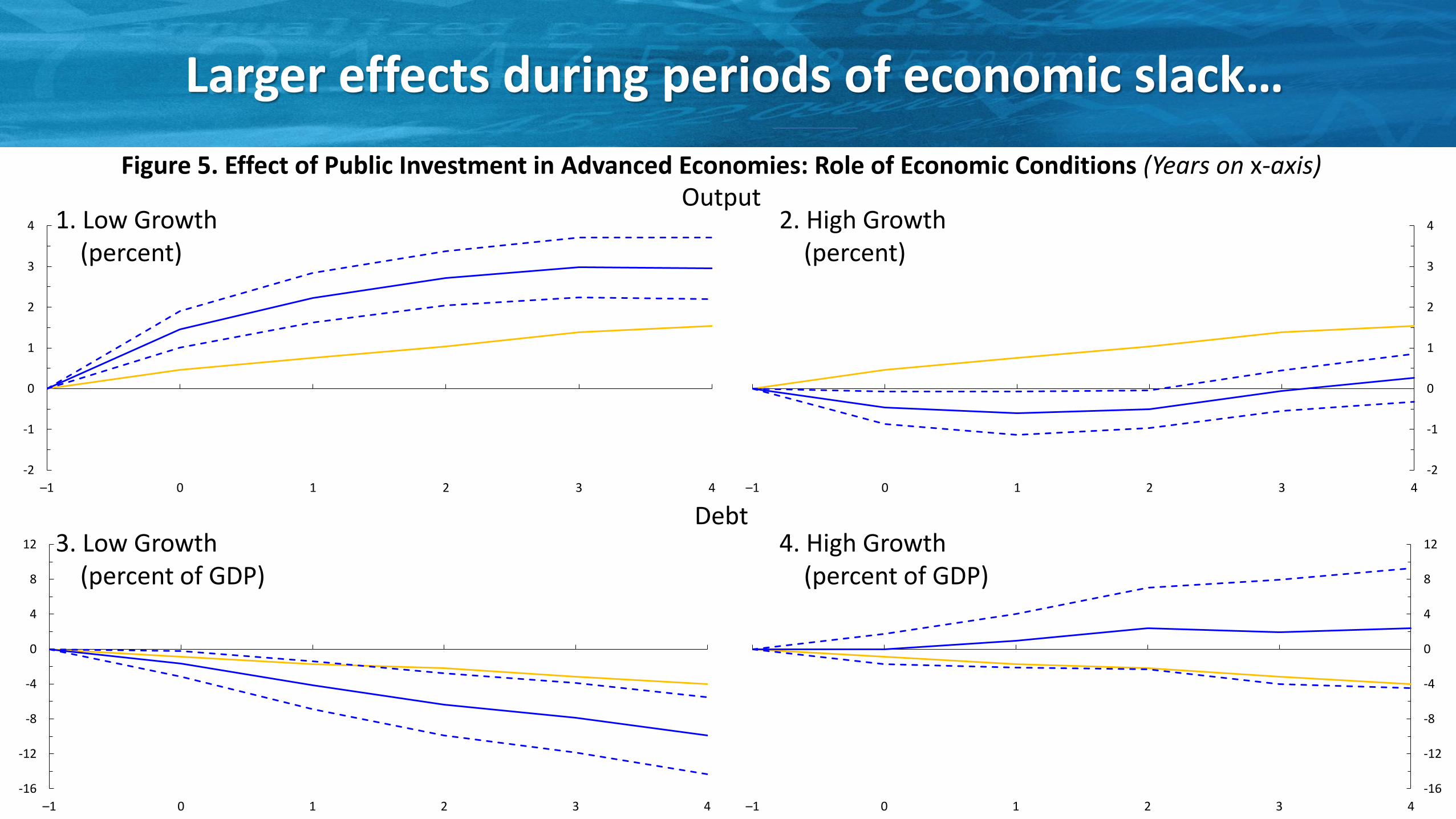
Larger effects during periods of economic slack…
-2
-1
0
1
2
3
4
–1 0 1 2 3 4
-2
-1
0
1
2
3
4
–1 0 1 2 3 4
-16
-12
-8
-4
0
4
8
12
–1 0 1 2 3 4
-16
-12
-8
-4
0
4
8
12
–1 0 1 2 3 4
Figure 5. Effect of Public Investment in Advanced Economies: Role of Economic Conditions (Years on x-axis)
1. Low Growth (percent)
2. High Growth (percent)
Output
Debt 3. Low Growth (percent of GDP)
4. High Growth (percent of GDP)

…and in countries with greater efficiency…
-1
0
1
2
3
4
–1 0 1 2 3 4
-1
0
1
2
3
4
–1 0 1 2 3 4
-16
-12
-8
-4
0
4
8
12
–1 0 1 2 3 4
-16
-12
-8
-4
0
4
8
12
–1 0 1 2 3 4
Figure 6. Effect of Public Investment in Advanced Economies: Role of Efficiency (Years on x-axis)
1. High Efficiency (percent)
2. Low Efficiency (percent)
Output
Debt 3. High Efficiency (percent of GDP)
4. Low Efficiency (percent of GDP)

…and when is debt financed
-2
-1
0
1
2
3
4
5
6
–1 0 1 2 3 4
-2
-1
0
1
2
3
4
5
6
–1 0 1 2 3 4
-20
-16
-12
-8
-4
0
4
8
–1 0 1 2 3 4
-20
-16
-12
-8
-4
0
4
8
–1 0 1 2 3 4
Figure 7. Effect of Public Investment in Advanced Economies: Role of Mode of Financing (Years on x-axis)
1. Debt Financed (percent)
2. Budget Neutral (percent)
Output
Debt 3. Debt Financed (percent of GDP)
4. Budget Neutral (percent of GDP)

Macroeconomic Effects of Public Investment in EMs and LICs: Empirical Evidence

Empirical strategy
Three complementary approaches 1.Describe the evolution of key macroeconomic variables surrounding public investment booms (Warner, 2014) 2.Identify exogenous shocks to public investment as residuals from an estimated spending rule (Corsetti, Meier and Muller, 2012)
3.Instrument public investment with the predetermined component of disbursement on loans from official creditors to developing countries (Eden and Kraay, 2014)

Public investment booms identified as large increases in government investment spending
0
1
2
3
4
5
6
7
8
9
-1 0 1 2 3 4 5 6 7 8 9 10
Figure 8. Public Investment (percent of GDP)
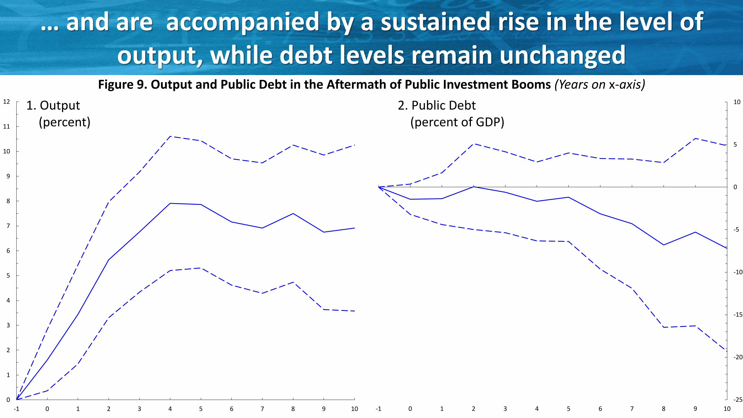
… and are accompanied by a sustained rise in the level of output, while debt levels remain unchanged
0
1
2
3
4
5
6
7
8
9
10
11
12
-1 0 1 2 3 4 5 6 7 8 9 10
2. Public Debt (percent of GDP)
-25
-20
-15
-10
-5
0
5
10
-1 0 1 2 3 4 5 6 7 8 9 10
1. Output (percent)
Figure 9. Output and Public Debt in the Aftermath of Public Investment Booms (Years on x-axis)

Public investment has a positive, long lasting effect on output in EMs and LICs.
1. Public Investment Shocks Derived from Fiscal Policy Rule 2. Public Investment Instrumented by Official Loan Disbursement
-2
-1
0
1
2
3
4
5
-1 0 1 2 3 4
-2
-1
0
1
2
3
4
5
-1 0 1 2 3 4
Figure 9. Effect of Public Investment on Output in Emerging Market and Developing Economies (Percent; years on x-axis)
Summary of empirical findings on macroeconomic effects of public investment
Public investment has a positive and long lasting effect on the level of output. No evidence of rising levels of public debt or crowding out private investment. Macroeconomic response is shaped by: • Degree of economic slack: positive output effects are more pronounced when public investment is undertaken during periods of economic slack. • Efficiency of public investment: countries with greater efficiency of public investment get a bigger bang for their buck. • How public investment is financed: Public investment has larger output effects when it is financed by issuing debt rather than by raising taxes or cutting other spending.

Macroeconomic Effects of Public Investment: Model Simulations

Current scenario for AEs
0
0.5
1
1.5
2
2.5
3
2013 14 15 16 17 18 19 20 21 22 23
0
1
2
3
4
2013 14 15 16 17 18 19 20 21 22 23
-4
-3
-2
-1
0
1
2013 14 15 16 17 18 19 20 21 22 23
1. Output (percent deviation from baseline)
2. Debt (percentage-point-of-GDP deviation from baseline)
3. Private Investment (percent deviation from baseline)
Figure 10. Model Simulations: Effect of Public Investment in Advanced Economies in the Current Scenario
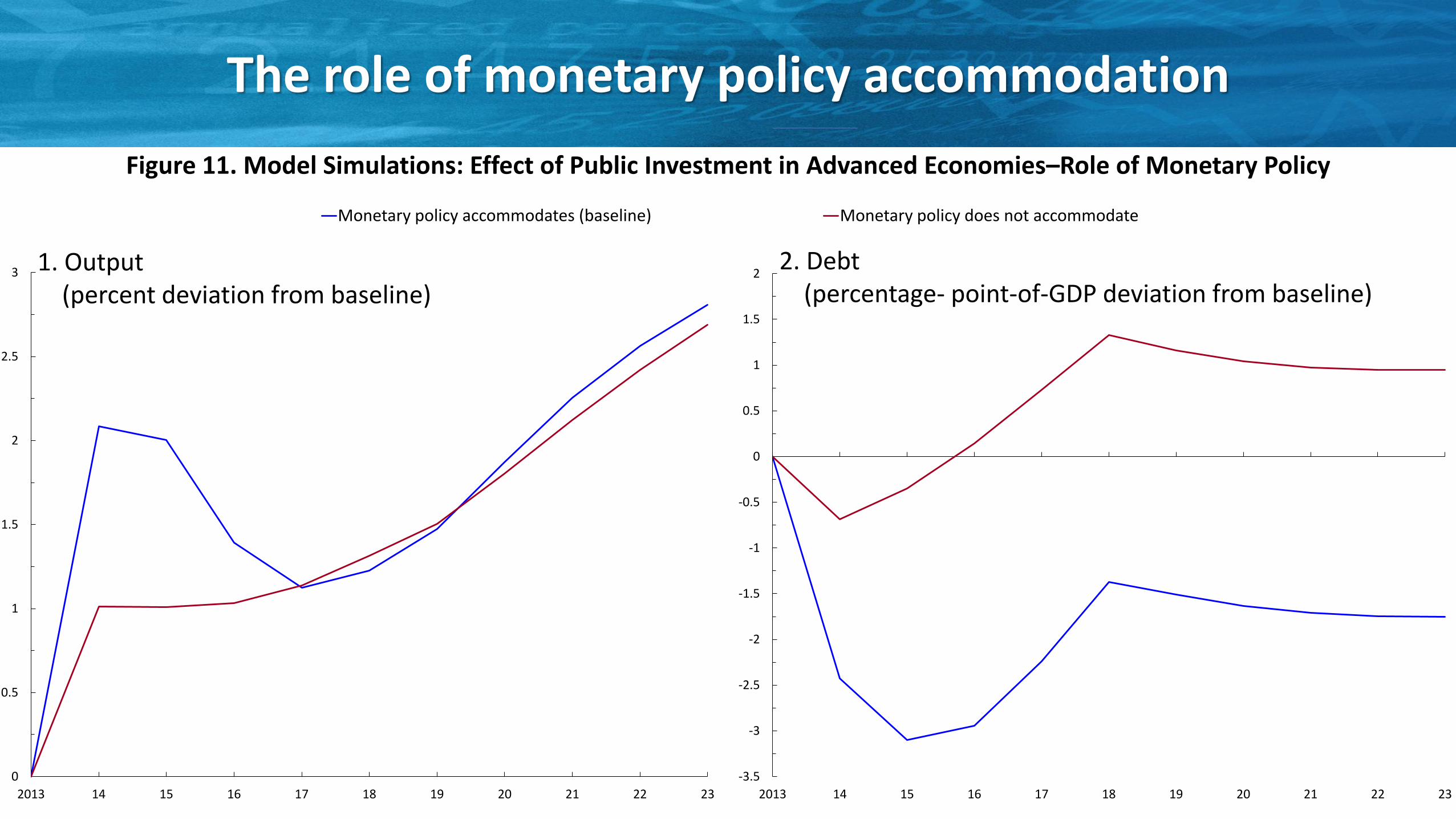
Monetary policy accommodates (baseline) Monetary policy does not accommodate
The role of monetary policy accommodation
0
0.5
1
1.5
2
2.5
3
2013 14 15 16 17 18 19 20 21 22 23
-3.5
-3
-2.5
-2
-1.5
-1
-0.5
0
0.5
1
1.5
2
2013 14 15 16 17 18 19 20 21 22 23
1. Output (percent deviation from baseline)
2. Debt (percentage- point-of-GDP deviation from baseline)
Figure 11. Model Simulations: Effect of Public Investment in Advanced Economies–Role of Monetary Policy
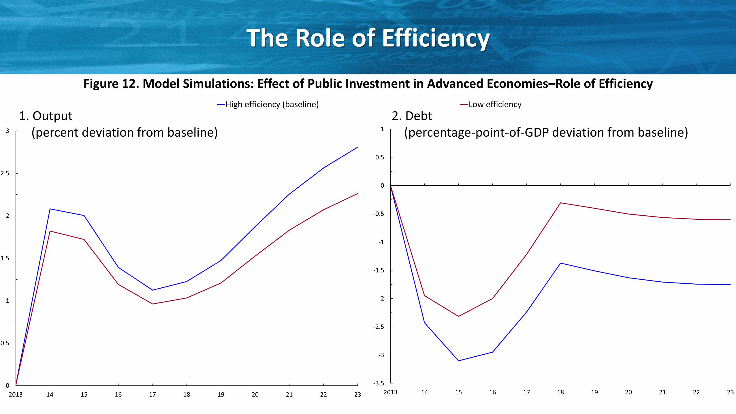
High efficiency (baseline) Low efficiency
The Role of Efficiency
0
0.5
1
1.5
2
2.5
3
2013 14 15 16 17 18 19 20 21 22 23
-3.5
-3
-2.5
-2
-1.5
-1
-0.5
0
0.5
1
2013 14 15 16 17 18 19 20 21 22 23
1. Output (percent deviation from baseline)
2. Debt (percentage-point-of-GDP deviation from baseline)
Figure 12. Model Simulations: Effect of Public Investment in Advanced Economies–Role of Efficiency

Base line Low return High return
Return on Public Capital
0
0.5
1
1.5
2
2.5
3
3.5
2013 14 15 16 17 18 19 20 21 22 23
-4
-3.5
-3
-2.5
-2
-1.5
-1
-0.5
0
0.5
2013 14 15 16 17 18 19 20 21 22 23
1. Output (percent deviation from baseline)
2. Debt (percentage-point-of-GDP deviation from baseline)
Figure 13. Model Simulations: Effect of Public Investment in Advanced Economies–Role of Return on Public Capital
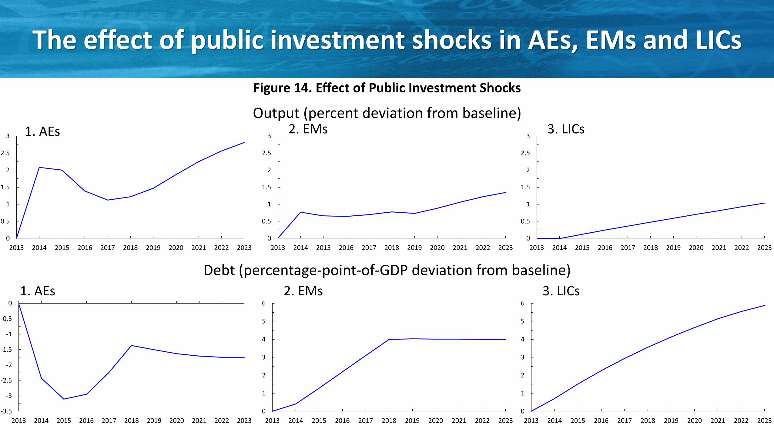
The effect of public investment shocks in AEs, EMs and LICs
0
0.5
1
1.5
2
2.5
3
2013 2014 2015 2016 2017 2018 2019 2020 2021 2022 2023
0
0.5
1
1.5
2
2.5
3
2013 2014 2015 2016 2017 2018 2019 2020 2021 2022 2023
0
0.5
1
1.5
2
2.5
3
2013 2014 2015 2016 2017 2018 2019 2020 2021 2022 2023
-3.5
-3
-2.5
-2
-1.5
-1
-0.5
0
2013 2014 2015 2016 2017 2018 2019 2020 2021 2022 2023
0
1
2
3
4
5
6
2013 2014 2015 2016 2017 2018 2019 2020 2021 2022 2023
0
1
2
3
4
5
6
2013 2014 2015 2016 2017 2018 2019 2020 2021 2022 2023
1. AEs 2. EMs 3. LICs
1. AEs 2. EMs 3. LICs
Output (percent deviation from baseline)
Debt (percentage-point-of-GDP deviation from baseline)
Figure 14. Effect of Public Investment Shocks

Summary of simulation findings on macroeconomic effects of public investment
AEs •Public Investment has a positive and long lasting effect on the level of output •Evidence of a decrease in the level of public debt and crowding in of private investment •Larger macroeconomic responses in periods of economic slack [mp accommodates] and for greater efficiency of public investment
EMs and LICs • Public Investment has a positive and long lasting effect on the level of output, but lower effects compared to AEs • Lower efficiency of public investment leads to a trade-off between higher output and debt

Policy Implications

The time is right for an infrastructure push
• For economies with clearly identified infrastructure needs and efficient public investment processes and where there is economic slack and monetary accommodation, there is a strong case for increasing public infrastructure spending.
• For these economies, the positive effects on output of increasing public infrastructure investment actually lead to a decline in public-debt-to-GDP ratios.
• Increasing the efficiency of public investment is critical to reap its full benefits. Thus, the key priority for economies with relatively low efficiency of public investment should be to raise the quality of infrastructure investment through better project appraisal, selection, and execution.

Thank you

The stock of public capital per capita is still much higher in AEs than in EMDEs...
0
5,000
10,000
15,000
20,000
25,000
30,000
Adv. Asia North America Adv. Europe Em. and Dev. Europe MENAP CIS LAC Em. and Dev. Asia SSA
Figure 15. Real Per Capita Public Capital Stock, 2010 (2005 PPP dollars per person)

There is a strong correlation between public capital and physical measures of infrastructure across countries.
y = 0.7295x - 5.2297
-3
-2
-1
0
1
2
3
4
5
5 6 7 8 9 10 11 12
Infr
astr
uct
ure
pe
r ca
pit
a
Log of real public capital stock per capita
Figure 16. Infrastructure and Real Public Capital Stock per capita (average, 2005–11)
Infra stocks
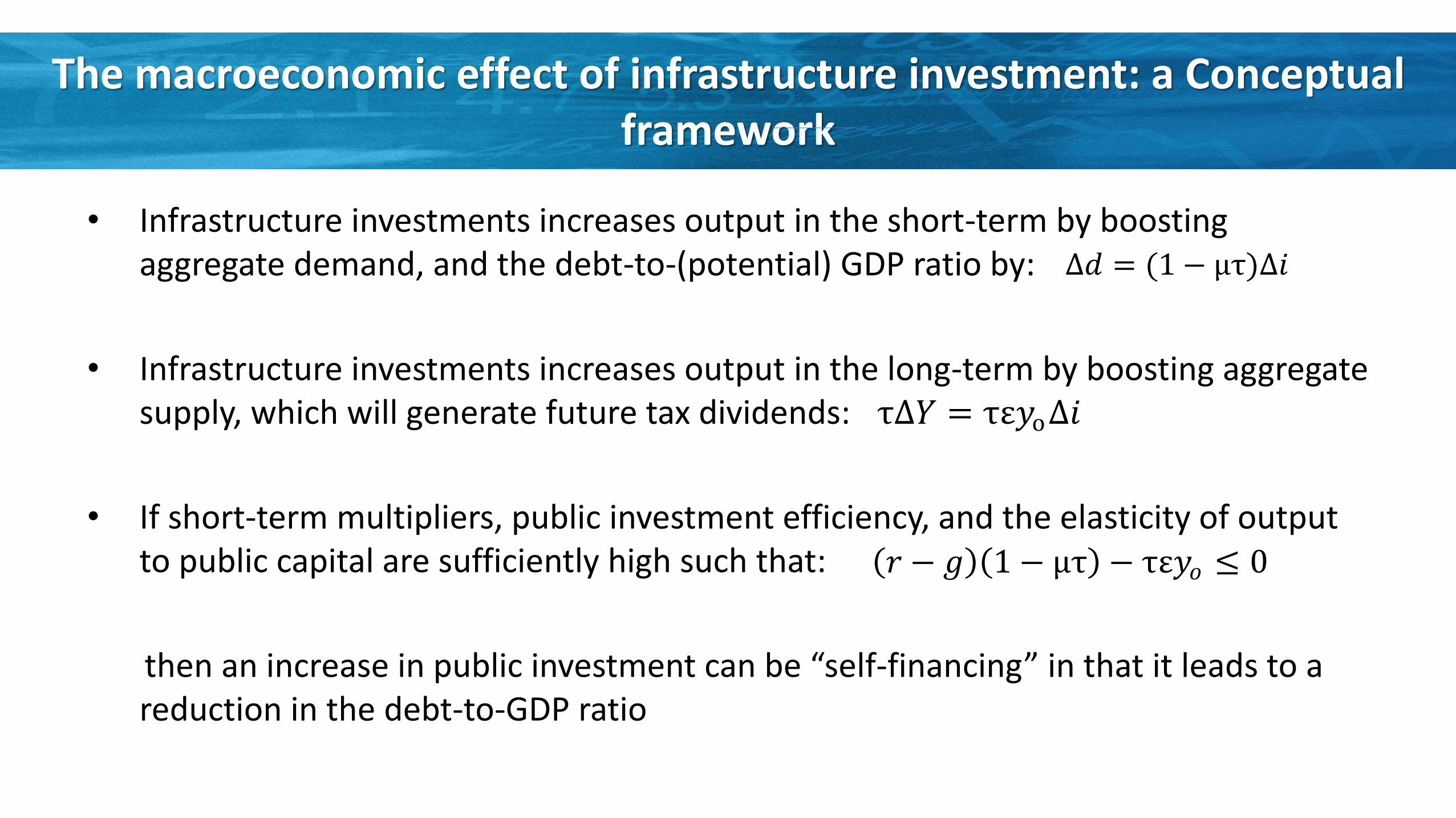
The macroeconomic effect of infrastructure investment: a Conceptual framework
• Infrastructure investments increases output in the short-term by boosting aggregate demand, and the debt-to-(potential) GDP ratio by:
• Infrastructure investments increases output in the long-term by boosting aggregate supply, which will generate future tax dividends:
• If short-term multipliers, public investment efficiency, and the elasticity of output to public capital are sufficiently high such that:
then an increase in public investment can be “self-financing” in that it leads to a reduction in the debt-to-GDP ratio
∆𝑑 = (1 − μτ)∆𝑖
τ∆𝑌 = τε𝑦o∆𝑖
𝑟 − 𝑔 1 − μτ − τε𝑦𝑜 ≤ 0

Macroeconomic Effects of Public Investment Shocks in AEs
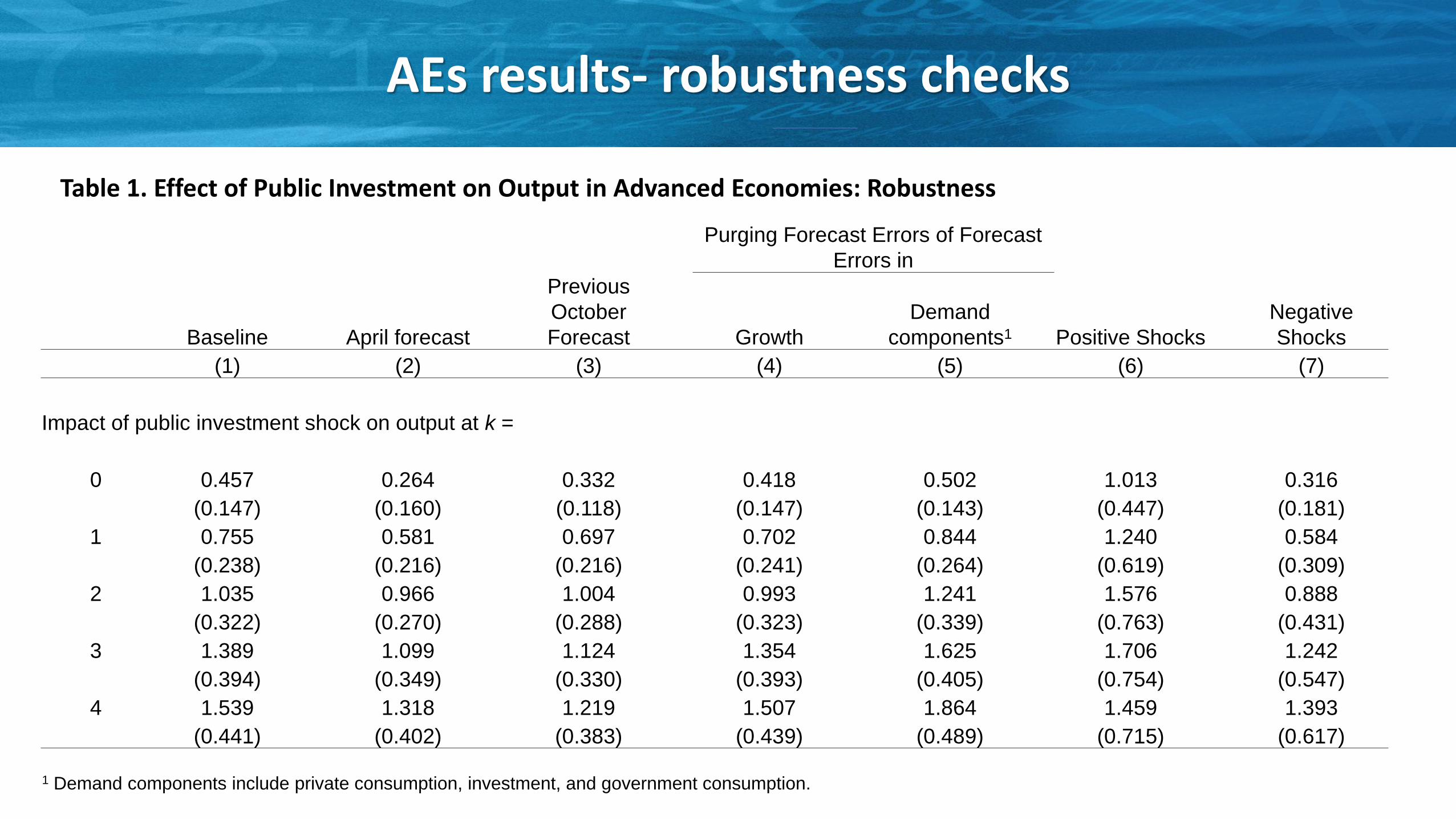
AEs results- robustness checks
Purging Forecast Errors of Forecast
Errors in
Baseline April forecast
Previous
October
Forecast Growth
Demand
components1 Positive Shocks
Negative
Shocks
(1) (2) (3) (4) (5) (6) (7)
Impact of public investment shock on output at k =
0 0.457 0.264 0.332 0.418 0.502 1.013 0.316
(0.147) (0.160) (0.118) (0.147) (0.143) (0.447) (0.181)
1 0.755 0.581 0.697 0.702 0.844 1.240 0.584
(0.238) (0.216) (0.216) (0.241) (0.264) (0.619) (0.309)
2 1.035 0.966 1.004 0.993 1.241 1.576 0.888
(0.322) (0.270) (0.288) (0.323) (0.339) (0.763) (0.431)
3 1.389 1.099 1.124 1.354 1.625 1.706 1.242
(0.394) (0.349) (0.330) (0.393) (0.405) (0.754) (0.547)
4 1.539 1.318 1.219 1.507 1.864 1.459 1.393
(0.441) (0.402) (0.383) (0.439) (0.489) (0.715) (0.617)
1 Demand components include private consumption, investment, and government consumption.
Table 1. Effect of Public Investment on Output in Advanced Economies: Robustness

AEs results- robustness checks
-1
0
1
2
3
4
–1 0 1 2 3 4 -0.5
0
0.5
1
1.5
2
2.5
–1 0 1 2 3 4
Figure 17. Effect of Public Investment Shocks on Output, Recessions vs. Expansions: Robustness Checks (Percent; years on x-axis)
1. Recessions 2. Expansions Recessions as Negative Growth Dummy
Recessions as Low Growth (as Actual) Dummy 3. Recessions 4. Expansions
-1
0
1
2
3
4
–1 0 1 2 3 4 0
0.5
1
1.5
2
2.5
–1 0 1 2 3 4

AEs results- robustness checks
Figure 18. Effect of Public Investment Shocks on Output, High vs. Low Efficiency: Robustness Checks (Percent; years on x-axis)
1. High Efficiency 2. Low Efficiency
-2
-1
0
1
2
3
4
5
–1 0 1 2 3 4
-2
-1
0
1
2
3
4
5
–1 0 1 2 3 4

AEs results- robustness checks
0
0.5
1
1.5
2
2.5
3
–1 0 1 2 3 4
Figure 19. Effect of Changes in Public Investment in Advanced Economies (Years on x-axis)
-4
-3
-2
-1
0
1
2
3
–1 0 1 2 3 4
-1.5
-1
-0.5
0
0.5
1
–1 0 1 2 3 4
1. Output (percent)
2. Debt (percent of GDP)
3. Private Investment (percent of GDP)

Distribution of public investment booms
0
1
2
3
4
5
6
7
0
1
2
3
4
5
6
7
Figure 20. Distribution of Public Investment Booms over Time (Number of Countries)
1. Advanced Economies 2. Emerging Market and Developing Economies
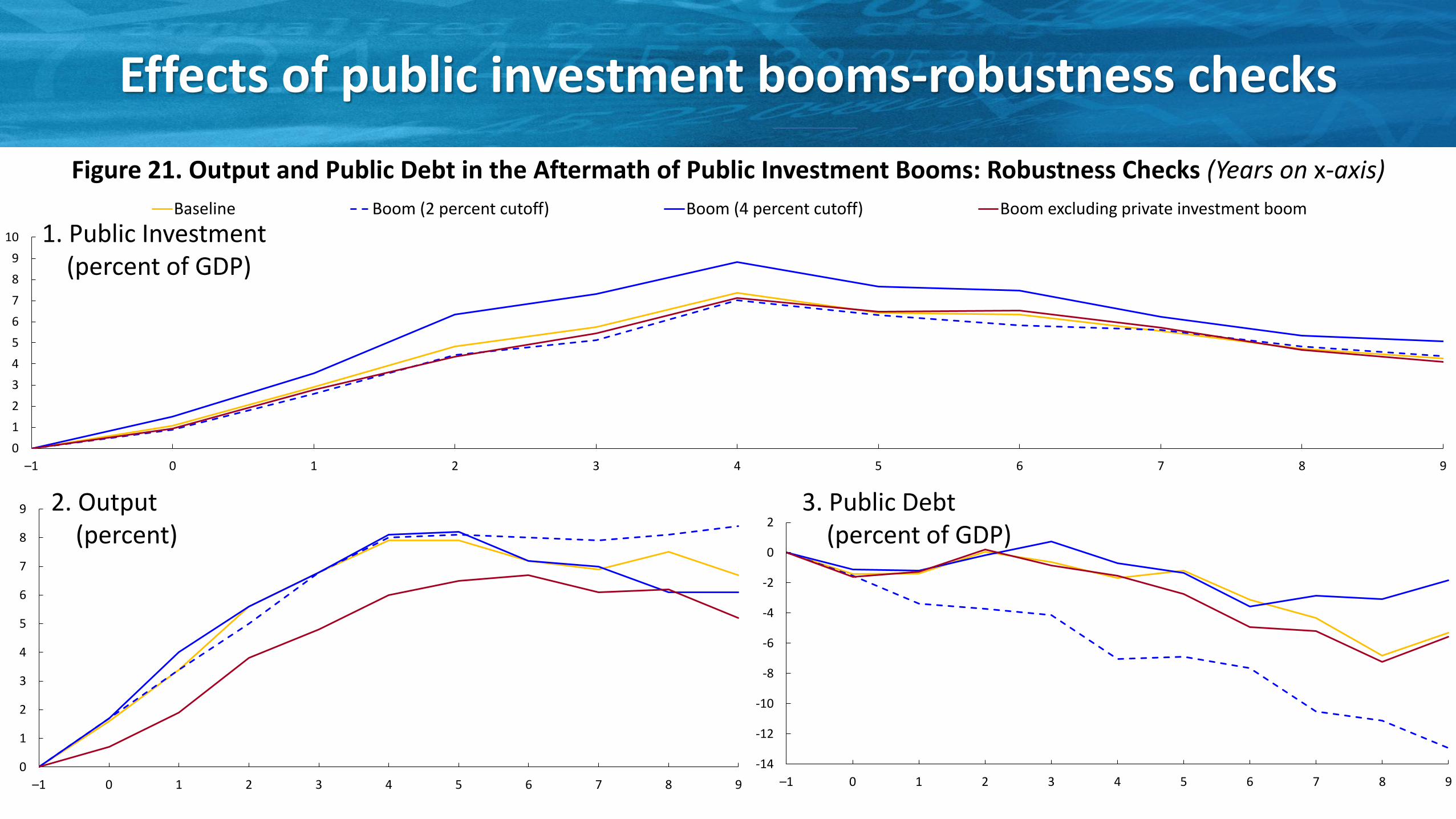
Baseline Boom (2 percent cutoff) Boom (4 percent cutoff) Boom excluding private investment boom
Effects of public investment booms-robustness checks
0
1
2
3
4
5
6
7
8
9
10
–1 0 1 2 3 4 5 6 7 8 9
0
1
2
3
4
5
6
7
8
9
–1 0 1 2 3 4 5 6 7 8 9
-14
-12
-10
-8
-6
-4
-2
0
2
–1 0 1 2 3 4 5 6 7 8 9
Figure 21. Output and Public Debt in the Aftermath of Public Investment Booms: Robustness Checks (Years on x-axis)
1. Public Investment (percent of GDP)
2. Output (percent)
3. Public Debt (percent of GDP)

Baseline Non–commodity exporters Commodity exporters Excluding booms preceded by terms-of-trade increases
Effects of public investment booms-robustness checks
0
1
2
3
4
5
6
7
8
9
10
–1 0 1 2 3 4 5 6 7 8 9
0
1
2
3
4
5
6
7
8
9
10
–1 0 1 2 3 4 5 6 7 8 9
-25
-20
-15
-10
-5
0
5
10
–1 0 1 2 3 4 5 6 7 8 9
Figure 22. Output and Public Debt in the Aftermath of Public Investment Booms: Role of Natural Resources (Years on x-axis)
1. Public Investment (percent of GDP)
2. Output (percent)
3. Public Debt (percent of GDP)

Table 2. Effect of Public Investment on Output in Emerging Market and Developing Economies: Public
Investment Shocks Derived from a Fiscal Policy Rule
Effects of public investment in EMDEs-robustness checks
Baseline 1/ Full sample
Top and Bottom 5 Percent of Shocks
Trimmed
k Coefficient SE Coefficient SE Coefficient SE
(1) (2) (3) (4) (5) (6)
–1 0 0 0 0 0 0
0 0.252 (0.066) 0.144 (0.074) 0.324 (0.100)
1 0.340 (0.096) 0.193 (0.086) 0.571 (0.142)
2 0.331 (0.126) 0.187 (0.100) 0.567 (0.191)
3 0.384 (0.152) 0.225 (0.119) 0.728 (0.238)
4 0.497 (0.189) 0.239 (0.174) 1.010 (0.313) Note: Columns (1), (3), and (5) present the estimated coefficients on the public investment shock from a series of regression estimates for each k in {0,4}.
Standard errors (SEs) of the estimated coefficients, which are shown in columns (2), (4), and (6), are corrected for heteroscedasticity and clustered at the
country level. There are 128 economies in the sample, with data from 1990–2013. All regressions include a full set of country and year fixed effects. k =
0 is the year of the shock.
1In the baseline specification, the top and bottom 1 percent of public investment shocks are trimmed.
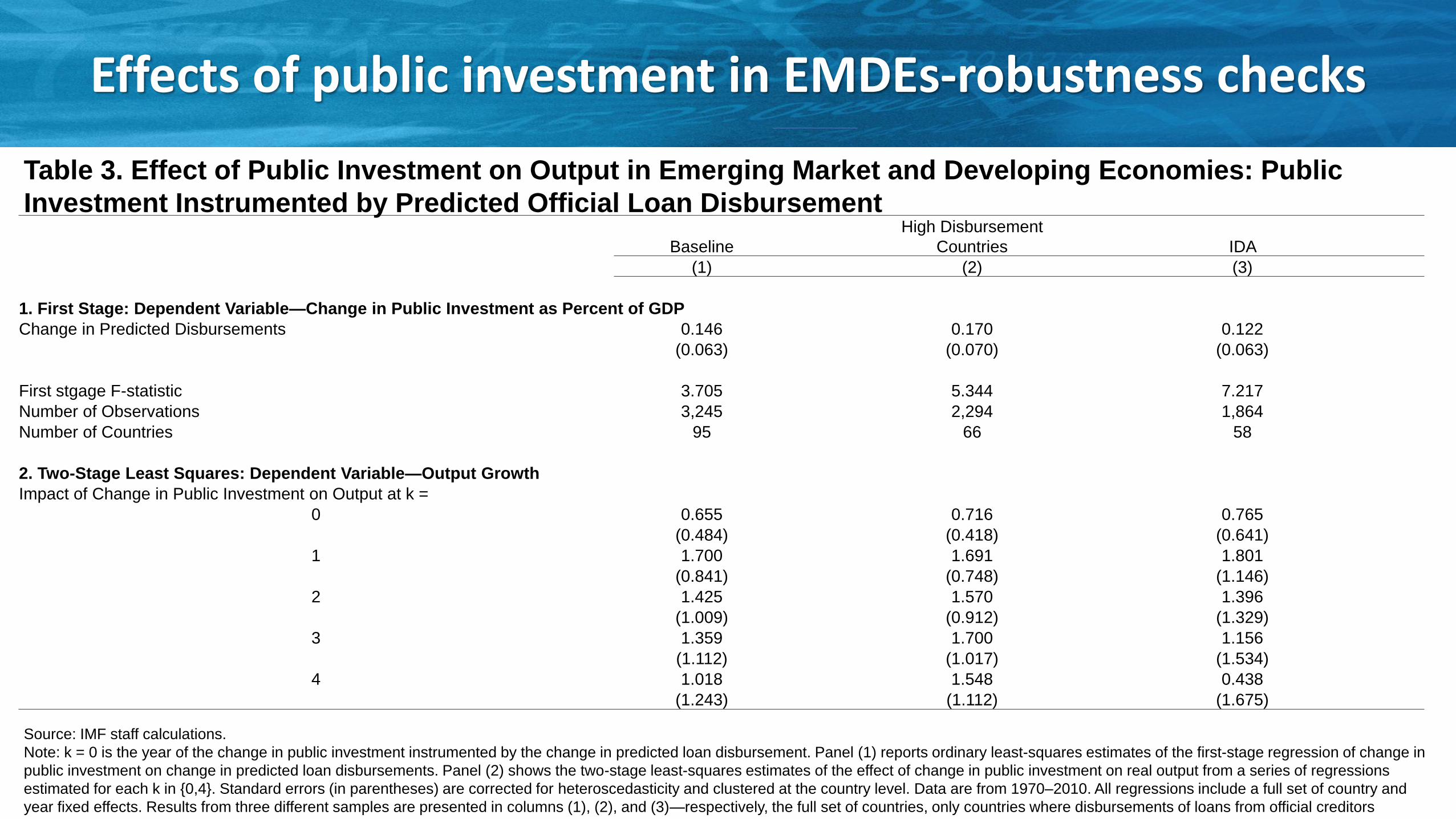
Table 3. Effect of Public Investment on Output in Emerging Market and Developing Economies: Public
Investment Instrumented by Predicted Official Loan Disbursement
Effects of public investment in EMDEs-robustness checks
Baseline
High Disbursement
Countries IDA
(1) (2) (3)
1. First Stage: Dependent Variable—Change in Public Investment as Percent of GDP
Change in Predicted Disbursements 0.146 0.170 0.122
(0.063) (0.070) (0.063)
First stgage F-statistic 3.705 5.344 7.217
Number of Observations 3,245 2,294 1,864
Number of Countries 95 66 58
2. Two-Stage Least Squares: Dependent Variable—Output Growth
Impact of Change in Public Investment on Output at k =
0 0.655 0.716 0.765
(0.484) (0.418) (0.641)
1 1.700 1.691 1.801
(0.841) (0.748) (1.146)
2 1.425 1.570 1.396
(1.009) (0.912) (1.329)
3 1.359 1.700 1.156
(1.112) (1.017) (1.534)
4 1.018 1.548 0.438
(1.243) (1.112) (1.675)
Source: IMF staff calculations.
Note: k = 0 is the year of the change in public investment instrumented by the change in predicted loan disbursement. Panel (1) reports ordinary least-squares estimates of the first-stage regression of change in
public investment on change in predicted loan disbursements. Panel (2) shows the two-stage least-squares estimates of the effect of change in public investment on real output from a series of regressions
estimated for each k in {0,4}. Standard errors (in parentheses) are corrected for heteroscedasticity and clustered at the country level. Data are from 1970–2010. All regressions include a full set of country and
year fixed effects. Results from three different samples are presented in columns (1), (2), and (3)—respectively, the full set of countries, only countries where disbursements of loans from official creditors
average at least 10 percent of total government spending, and only countries eligible for International Development Association (IDA) support.

Macroeconomic Effects of Public Investment Shocks- Model Simulations
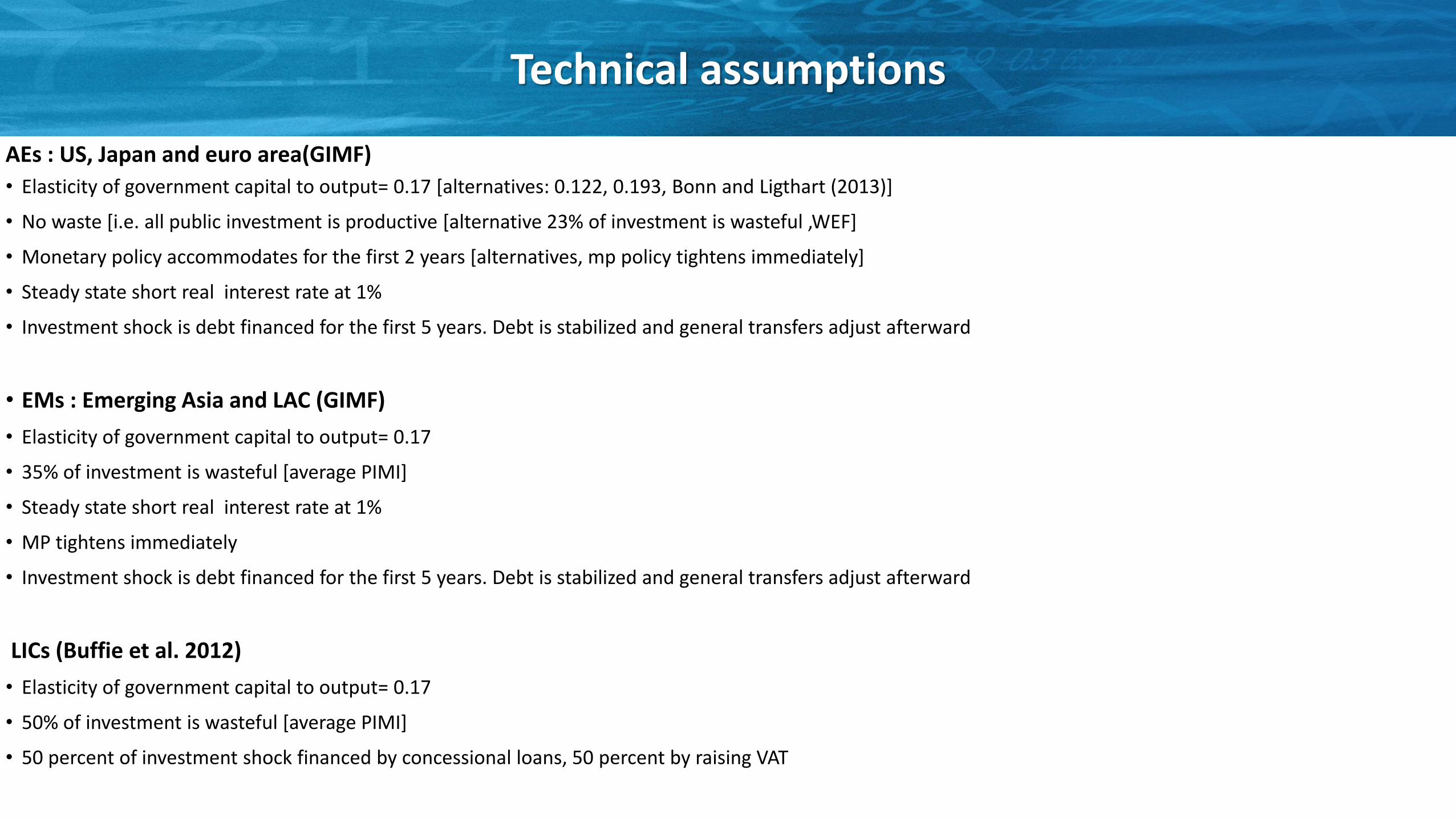
Technical assumptions
AEs : US, Japan and euro area(GIMF)
• Elasticity of government capital to output= 0.17 [alternatives: 0.122, 0.193, Bonn and Ligthart (2013)]
• No waste [i.e. all public investment is productive [alternative 23% of investment is wasteful ,WEF]
• Monetary policy accommodates for the first 2 years [alternatives, mp policy tightens immediately]
• Steady state short real interest rate at 1%
• Investment shock is debt financed for the first 5 years. Debt is stabilized and general transfers adjust afterward
• EMs : Emerging Asia and LAC (GIMF)
• Elasticity of government capital to output= 0.17
• 35% of investment is wasteful [average PIMI]
• Steady state short real interest rate at 1%
• MP tightens immediately
• Investment shock is debt financed for the first 5 years. Debt is stabilized and general transfers adjust afterward
LICs (Buffie et al. 2012)
• Elasticity of government capital to output= 0.17
• 50% of investment is wasteful [average PIMI]
• 50 percent of investment shock financed by concessional loans, 50 percent by raising VAT

Current scenario for US, EA, Japan
0
0.5
1
1.5
2
2.5
3
3.5
4
2013 14 15 16 17 18 19 20 21 22 23
0
0.5
1
1.5
2
2.5
3
3.5
4
2013 14 15 16 17 18 19 20 21 22 23
0
0.5
1
1.5
2
2.5
3
3.5
4
2013 14 15 16 17 18 19 20 21 22 23
-7
-6
-5
-4
-3
-2
-1
0
2013 14 15 16 17 18 19 20 21 22 23
-7
-6
-5
-4
-3
-2
-1
0
2013 14 15 16 17 18 19 20 21 22 23
-7
-6
-5
-4
-3
-2
-1
0
2013 14 15 16 17 18 19 20 21 22 23
1. US 2. EA 3. Japan
4. US 5. EA 6. Japan
Output (percent deviation from baseline)
Debt (percentage-point-of-GDP deviation from baseline)
Figure 23. Effect of Public Investment in US, Euro Area, and Japan in the Current Scenario

The Role of Fiscal Institutions
-2
-1.8
-1.6
-1.4
-1.2
-1
-0.8
-0.6
-0.4
-0.2
0
Strong Planning Institutions Medium Plannning Institutions Weak Planning Institutions
Figure 24. Protection of Capital Expenditure (change in public investment; percent of total spending, 2010-12)
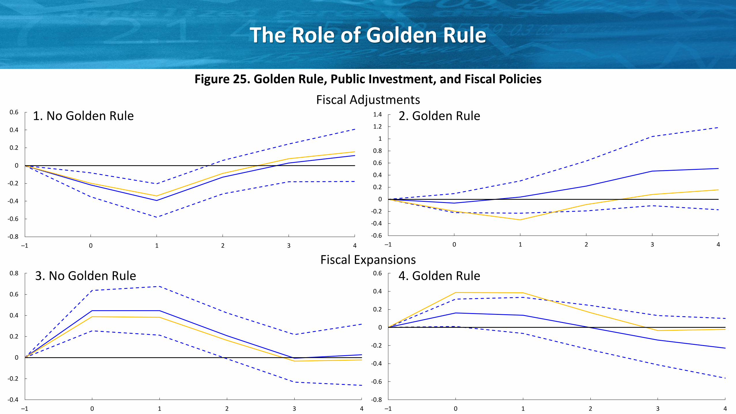
The Role of Golden Rule
Figure 25. Golden Rule, Public Investment, and Fiscal Policies
-0.8
-0.6
-0.4
-0.2
0
0.2
0.4
0.6
–1 0 1 2 3 4
1. No Golden Rule
-0.6
-0.4
-0.2
0
0.2
0.4
0.6
0.8
1
1.2
1.4
–1 0 1 2 3 4
-0.4
-0.2
0
0.2
0.4
0.6
0.8
–1 0 1 2 3 4
-0.8
-0.6
-0.4
-0.2
0
0.2
0.4
0.6
–1 0 1 2 3 4
3. No Golden Rule 4. Golden Rule
2. Golden Rule
Fiscal Expansions
Fiscal Adjustments


