
Ple
ase
note
tha
t th
is is a
n a
uth
or-
pro
du
ce
d P
DF
of
an a
rtic
le a
cce
pte
d fo
r p
ub
lica
tio
n fo
llow
ing
pe
er
revie
w. T
he d
efin
itiv
e p
ublis
he
r-au
the
ntica
ted
ve
rsio
n is a
va
ilab
le o
n t
he p
ublis
her
We
b s
ite
1
Science February 2005, Volume 307 (5712), Pages 1088-1091 http://dx.doi.org/10.1126/science.1105692 © 2012 American Association for the Advancement of Science. All Rights Reserved.
Archimer http://archimer.ifremer.fr
Iron Isotope Constraints on the Archean and Paleoproterozoic Ocean Redox State
Olivier J. Rouxel
1, *, Andrey Bekker
2 and Katrina J. Edwards
1
1 Marine Chemistry and Geochemistry Department, Geomicrobiology Group, Woods Hole Oceanographic
Institution, Mail Stop 8, Woods Hole, MA 02543, USA. 2 Geophysical Laboratory, Carnegie Institution of Washington, 5251 Broad Branch Road NW, Washington, DC
20015, USA.
*: Corresponding author : Olivier J. Rouxel, email address : [email protected]
Abstract : The response of the ocean redox state to the rise of atmospheric oxygen about 2.3 billion years ago (Ga) is a matter of controversy. Here we provide iron isotope evidence that the change in the ocean iron cycle occurred at the same time as the change in the atmospheric redox state. Variable and negative iron isotope values in pyrites older than about 2.3 Ga suggest that an iron-rich global ocean was strongly affected by the deposition of iron oxides. Between 2.3 and 1.8 Ga, positive iron isotope values of pyrite likely reflect an increase in the precipitation of iron sulfides relative to iron oxides in a redox stratified ocean.
The rise of atmospheric oxygen, which began by about 2.3 Ga (1–3), was one of the most important changes in Earth's history. Because Fe, along with C and S, are linked to and maintain the redox state of the surface environment, the concentration and isotopic composition of Fe in seawater were likely affected by the change in the redox state of the atmosphere. The rise of atmospheric oxygen should have also led to dramatic changes in the ocean Fe cycle because of the high reactivity of Fe with oxygen. However, deposition of banded iron formations (BIFs) during the Paleoproterozoic era suggests that the deep ocean remained anoxic, at least episodically, until about 1.8 Ga, which allowed high concentrations of Fe(II) to accumulate in the deep waters (4).
Here we use Fe isotope systematics (5) to provide constraints on the redox state of the Archean and Paleoproterozoic oceans and to identify direct links between the oxidation of the atmosphere and the Fe ocean cycle. Laboratory and field studies suggest that Fe isotope variations are associated mainly with redox changes (6, 7). Lithogenic sources of Fe on the modern oxygenated Earth, such as weathering products, continental sediments, river loads, and marine sediments, have isotopic compositions similar to those of igneous rocks (8, 9). In contrast,

3
seafloor hydrothermal sulfides and secondary Fe-bearing minerals from the altered oceanic crust
span nearly the entire measured range of δ56Fe (5) on Earth from -2.1 to 1.3‰ (10, 11). Large
variations of δ56Fe (from -2.5 to 1.0‰) in Late Archean to Early Paleoproterozoic BIF have been
also reported (12) highlighting the roles of ferrous Fe oxidation, fluid-mineral isotope
fractionation, and potentially microbial processes in the fractionation of Fe isotopes.
Study of S isotope composition of sedimentary pyrite over geological time has placed
important constraints on the S cycle and the evolution of ocean chemistry (13) and here we apply
a similar time-record approach to explore potential change in Fe isotope compositions. Pyrite
formation in modern organic-rich marine sediments is mediated by sulfate-reducing bacteria and
proceeds essentially through the dissolution and reduction of lithogenic Fe-oxides and Fe-
silicates to Fe(II), either below the sediment-water interface or in stratified euxinic bottom waters
(14-16). During reduction of Fe-oxides, diagenetic fluids with isotopically light Fe(II) may be
produced (17, 18). However, the Fe isotope composition of sedimentary pyrite from Phanerozoic
organic-rich sediments studied so far (Fig.1, Table S2, 19) suggests that such processes are
unlikely to produce sedimentary pyrite with δ56Fe < -0.5‰. Presumably, most of reactive Fe is
scavenged to form pyrite, minimizing Fe isotope fractionation regardless of the isotope effect
during Fe reduction (17) and precipitation (20). In contrast, when high concentrations of Fe(II)
accumulate under anoxic conditions and low sulfide concentration, large δ56Fe variations (10-12)
may occur due to partial Fe(II) oxidation, Fe(III) reduction and distillation processes during
mineral precipitation. We thus hypothesize that Fe isotope variations in sedimentary pyrite are
particularly sensitive to the concentration of dissolved Fe(II) and can be used to place important
constraints on the sources and sinks of the Fe(II) reservoir.
4
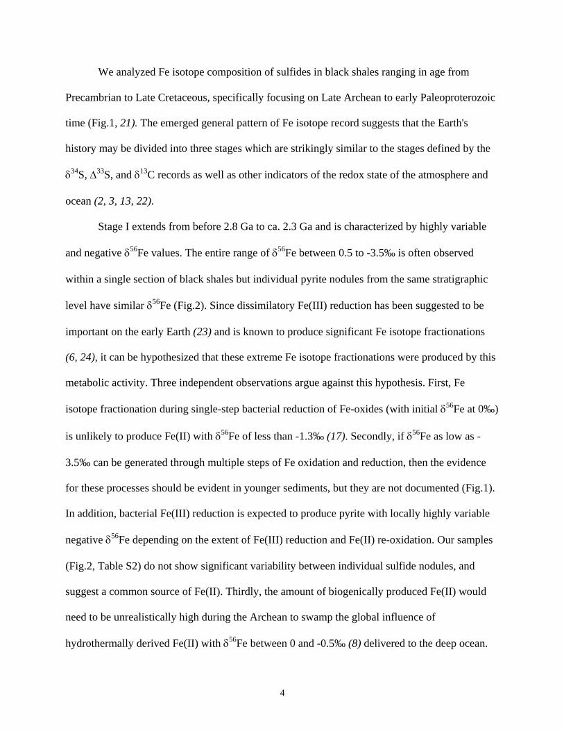
We analyzed Fe isotope composition of sulfides in black shales ranging in age from
Precambrian to Late Cretaceous, specifically focusing on Late Archean to early Paleoproterozoic
time (Fig.1, 21). The emerged general pattern of Fe isotope record suggests that the Earth's
history may be divided into three stages which are strikingly similar to the stages defined by the
δ34S, ∆33S, and δ13C records as well as other indicators of the redox state of the atmosphere and
ocean (2, 3, 13, 22).
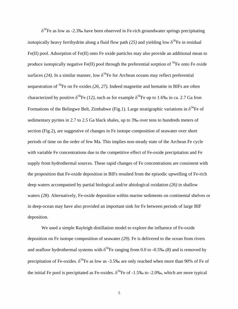
Stage I extends from before 2.8 Ga to ca. 2.3 Ga and is characterized by highly variable
and negative δ56Fe values. The entire range of δ56Fe between 0.5 to -3.5‰ is often observed
within a single section of black shales but individual pyrite nodules from the same stratigraphic
level have similar δ56Fe (Fig.2). Since dissimilatory Fe(III) reduction has been suggested to be
important on the early Earth (23) and is known to produce significant Fe isotope fractionations
(6, 24), it can be hypothesized that these extreme Fe isotope fractionations were produced by this
metabolic activity. Three independent observations argue against this hypothesis. First, Fe
isotope fractionation during single-step bacterial reduction of Fe-oxides (with initial δ56Fe at 0‰)
is unlikely to produce Fe(II) with δ56Fe of less than -1.3‰ (17). Secondly, if δ56Fe as low as -
3.5‰ can be generated through multiple steps of Fe oxidation and reduction, then the evidence
for these processes should be evident in younger sediments, but they are not documented (Fig.1).
In addition, bacterial Fe(III) reduction is expected to produce pyrite with locally highly variable
negative δ56Fe depending on the extent of Fe(III) reduction and Fe(II) re-oxidation. Our samples
(Fig.2, Table S2) do not show significant variability between individual sulfide nodules, and
suggest a common source of Fe(II). Thirdly, the amount of biogenically produced Fe(II) would
need to be unrealistically high during the Archean to swamp the global influence of
hydrothermally derived Fe(II) with δ56Fe between 0 and -0.5‰ (8) delivered to the deep ocean.
5
δ56Fe as low as -2.3‰ have been observed in Fe-rich groundwater springs precipitating
isotopically heavy ferrihydrite along a fluid flow path (25) and yielding low δ56Fe in residual
Fe(II) pool. Adsorption of Fe(II) onto Fe oxide particles may also provide an additional mean to
produce isotopically negative Fe(II) pool through the preferential sorption of 56Fe onto Fe oxide
surfaces (24). In a similar manner, low δ56Fe for Archean oceans may reflect preferential
sequestration of 56Fe on Fe oxides (26, 27). Indeed magnetite and hematite in BIFs are often
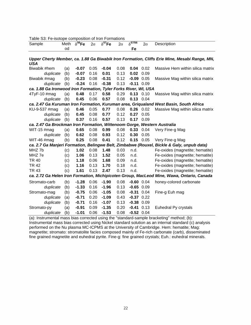
characterized by positive δ56Fe (12), such as for example δ56Fe up to 1.6‰ in ca. 2.7 Ga Iron
Formations of the Belingwe Belt, Zimbabwe (Fig.1). Large stratigraphic variations in δ56Fe of
sedimentary pyrites in 2.7 to 2.5 Ga black shales, up to 3‰ over tens to hundreds meters of
section (Fig.2), are suggestive of changes in Fe isotope composition of seawater over short
periods of time on the order of few Ma. This implies non-steady state of the Archean Fe cycle
with variable Fe concentrations due to the competitive effect of Fe-oxide precipitation and Fe
supply from hydrothermal sources. These rapid changes of Fe concentrations are consistent with
the proposition that Fe-oxide deposition in BIFs resulted from the episodic upwelling of Fe-rich
deep waters accompanied by partial biological and/or abiological oxidation (26) in shallow
waters (28). Alternatively, Fe-oxide deposition within marine sediments on continental shelves or
in deep-ocean may have also provided an important sink for Fe between periods of large BIF
deposition.
We used a simple Rayleigh distillation model to explore the influence of Fe-oxide
deposition on Fe isotope composition of seawater (29). Fe is delivered to the ocean from rivers
and seafloor hydrothermal systems with δ56Fe ranging from 0.0 to -0.5‰ (8) and is removed by
precipitation of Fe-oxides. δ56Fe as low as -3.5‰ are only reached when more than 90% of Fe of
the initial Fe pool is precipitated as Fe-oxides. δ56Fe of -1.5‰ to -2.0‰, which are more typical

6
of Late Archean sulfides, correspond to about 50% of Fe precipitated as oxides. This value is
similar to the estimates of Fe sink in BIFs based on P adsorption (30).
Stage II, covering the time interval from ca. 2.3 to ca. 1.7 Ga, is characterized by the
disappearance of negative δ56Fe and the emergence of positive δ56Fe up to 1.2‰. Major
perturbations in biogeochemical and climatic record occurred during the beginning of Stage II.
These include a) negative and positive carbon isotope excursions in carbonates sandwiched
between two glacial diamictites; b) Earth's earliest global glaciations; and c) oxidation of the
Earth's atmosphere as suggested by increasing seawater sulfate content inferred from the δ34S
record and appearance of sulfate evaporites, disappearance of non-mass dependent S isotope
fractionation, appearance of red beds, oxidized paleosols, hematitic oölites and pisolites, Mn-
oxide deposits, and Ce anomalies in chemical sedimentary deposits (3, 13, 22, 31). Strikingly, the
appearance of positive δ56Fe, persisting until ca 1.7 Ga, together with the disappearance of
strongly negative δ56Fe occur during the period when the most sensitive indicators for the rise of
atmospheric oxygen first appear. All these observations suggest that the oxidation of the surface
environment in the early Paleoproterozoic was relatively rapid and directly affected Fe isotope
composition of the ocean.
How the change in the Fe isotope record ca. 2.3 Ga ago corresponds with change of
oceanic Fe cycle and redox state of the ocean is not straightforward. Interestingly, large BIF
deposits are almost entirely lacking between 2.3 and 2.1 Ga (32) which is consistent with the lack
of negative δ56Fe during this period. However, BIF deposition returned at ca. 2.1 Ga and major
BIFs were deposited in North America and Australia (32). If δ56Fe of pyrites in black shales
deposited between 2.1 to 1.8 Ga are representative of the whole ocean, then BIF deposition
mechanisms were different from those prevailing during the Archean. We infer that late

7
Paleoproterozoic BIFs were deposited in an oxygenated layer of the ocean and complete
precipitation of Fe from Fe-rich plumes uplifting from the deep ocean did not affect Fe isotope
composition of the deep ocean. Despite the limited number of analyses, the narrow range of δ56Fe
of hematite and magnetite from the 1.88 Ga Biwabik and Tyler formations compared to Archean
BIFs (Fig. 1; Table S3) is consistent with this assumption.
An important consequence of the rise of atmospheric oxygen levels was the initiation of
oxidative weathering and an increase in sulfate delivery to seawater (13). Consequently, the
formation of Fe sulfides in the water column of pericratonic basins may have became the
dominant part of the global ocean Fe cycle and may have prevented deposition of large BIFs,
except during periods of intense submarine volcanic activity followed by high hydrothermal input
of Fe. The effect of the increased role of sulfide production on the Fe isotope record is presently
uncertain since reliable estimates of equilibrium Fe isotope fractionation during pyrite formation
are lacking (20). One plausible hypothesis is that the positive δ56Fe in 2.3 Ga to 1.8 Ga
sedimentary sulfides might be related to sulfide precipitation from a Fe-rich pool with δ56Fe
composition around 0‰ and a pyrite-Fe(II) fractionation factor of up to 1‰ as suggested in
previous studies (10, 33). This indicates that sulfide produced by sulfate reducing bacteria during
this period has been completely titrated by dissolved Fe species in the Fe-rich and sulfide-poor
ocean.
The disappearance of major BIFs after ca. 1.8 Ga is thought to indicate that the deep
ocean became either progressively oxic or euxinic (4). Since the solubility of Fe-sulfides and Fe-
oxides is low, most of hydrothermally-derived Fe(II) was likely rapidly precipitated in the deep
ocean allowing few possibilities to produce Fe isotope fractionation. The lack of significant δ56Fe
variations in sulfides from black shales younger than 1.5 Ga is thus consistent with the general

8
picture that the whole ocean was Fe-poor after ca. 1.6 Ga but do not place constraints on the oxic
vs. sulfidic nature of the deep ocean. Evidently, more data covering the Phanerozoic, Meso- and
Neoproterozoic time intervals are required to fully understand the change in ocean Fe cycle at ca.
1.8 Ga.
Our Fe isotope record provides new insights into the Archean and Paleoproterozoic ocean
chemistry and redox state. Fe isotopes suggest that the Archean oceans were globally Fe-rich,
their Fe isotope composition and Fe content were variable in response to the episodic
establishment of an Fe-rich pool supplied by hydrothermal activity and deposition of Fe-oxides,
either in BIFs or dispersed throughout sediments on continental shelves and in the deep sea. After
the rise of atmospheric oxygen by ca. 2.3 Ga, Paleoproterozoic ocean became stratified and
characterized by an increase of sulfide precipitation relative to Fe-oxide precipitation. During this
period, BIFs were likely deposited by upwelling of Fe(II)-rich plumes and rapid oxidation in the
oxygenated layer of the ocean. Conducting Fe isotope analyses of sedimentary sulfides in
conjunction with S isotope analyses should enable a more refined understanding of the origin of
the positive Fe isotope excursion and the biogeochemical cycles of Fe and S during the
Paleoproterozoic.

9
References and Notes
1. H. D. Holland, The Chemical Evolution of the Atmosphere and Oceans (Princeton Univ.
Press., New York, 1984).
2. J. Farquhar, H. Bao, M. Thiemens, Science 289, 756 (2000).
3. A. Bekker et al., Nature 427, 117 (2004).
4. The disappearance of BIFs after ca. 1.8 Ga has been initially thought to indicate the transition
to the oxygenated ocean (1) but a growing body of evidence suggests that sulfide, rather than
oxygen, could have been responsible for removing Fe from deep ocean waters (13, 34-36).
5. Data are reported using the delta notation relative to IRMM-14 Fe isotope reference standard
defined as δ56Fe=1000 * ( (56Fe/54Fe) sample / (56Fe/54Fe) IRMM-14 - 1). External precision of
δ56Fe are estimated at 0.10‰ (2σ level). Analytical procedures, sample descriptions and Fe
isotope composition of various georeference materials, black shales, and BIF are available as
supporting materials on Science Online.
6. C. M. Johnson, B. L. Beard, E. E. Roden, D. K. Newman, K. H. Nealson, Reviews in
Mineralogy and Geochemistry 55, 359 (2004).
7. B. L. Beard, C. M. Johnson, Reviews in Mineralogy and Geochemistry 55, 319 (2004).
8. B. L. Beard, C. M. Johnson, K. L. VonDamm, R. L. Poulson, Geology 31, 629 (2003).
9. The range of Fe isotope composition of hydrogenic ferromanganese deposits in modern
oceanic basins is significant (between -0.8‰ to -0.1‰ (37)), but it is unclear if the variability
is due to changes of Fe isotope composition in the water column or secondary effects.
10. O. Rouxel, Y. Fouquet, J. N. Ludden, Geochim. Cosmochim. Acta 68, 2295 (2004).
11. O. Rouxel, N. Dobbek, J. Ludden, Y. Fouquet, Chem. Geol. 202, 155 (2003).
10
12. C. M. Johnson, B. L. Beard, N. J. Beukes, C. Klein, J. M. O'Leary, Contrib. Mineral. Petrol.
144, 523 (2003).
13. D. E. Canfield, Science 396, 450 (1998).
14. D. E. Canfield, Geochim. Cosmochim. Acta 53, 619 (1989).
15. J. W. M. Wijsman, J. J. Middelburg, P. M. J. Herman, M. E. Bottcher, C. H. R. Heip, Mar.
Chem. 74, 261 (2001).
16. T. F. Anderson, R. Raiswell, Am. J. Sci. 304, 203 (2004).
17. Experimental studies suggest that Fe isotope fractionations during bacterial reduction of Fe
oxides is dependant on reduction rates (6). At high reduction rates, rapid formation and
sorption of Fe(II) to ferric oxide substrate produced fractionations as large as -2.3‰ but this
value corresponds to an extreme case and fractionation of -1.3‰ between biogenic Fe(II) and
ferric oxide is more representative (6).
18. S. Severmann, J. McManus, C. M. Johnson, B. L. Beard, Eos Trans. AGU, 84(52),
Ocean Sci. Meet. Suppl., Abstract OS31L-09, 2003
19. A. Matthews et al., Geochim. Cosmochim. Acta 68, 3107 (2004).
20. Theoretical calculations predict that pyrite (FeS2) is an isotopically heavy phase relative to
Fe(II) with a fractionation factor similar to magnetite (33). However, experimental
precipitation of mackinawite (Fe9S8) produces a kinetic isotope fractionation of 0.3‰ (38)
suggesting that the fractionation of pyrite is poorly constrained from -0.3 to 1.0‰ relative to
dissolved Fe(II).
21. Samples from different black shale units of similar ages were selected to distinguish between
local and global effects on Fe isotope composition of seawater. We extracted between 10 to
20 sulfide grains to obtain a best estimate for the average δ56Fe value for each sample. For
11
comparison and to evaluate heterogeneity, we also analyzed several individual sulfide
nodules from the same samples (Table S2).
22. J. A. Karhu, H. D. Holland, Geology 24, 867 (1996).
23. M. Vargas, K. Kashefi, E. L. Blunt-Harris, D. R. Lovley, Nature 395, 65 (1998).
24. G. A. Icopini, A. D. Anbar, S. S. Ruebush, M. Tien, S. L. Brantley, Geology 32, 205 (2004).
25. T. D. Bullen, A. F. White, C. W. Childs, D. V. Vivit, M. S. Schulz, Geology 29, 699 (2001).
26. Since the atmosphere was still reducing during this period, the mechanisms by which
oxidation of ferrous Fe sources occurred are extensively debated. Biogeochemical evidence
for oxygenic photosynthesis exists in sediments as old as 2.7 Ga (39) and may have
contributed to ferrous iron oxidation with O2. Alternatively, a direct mechanism for Fe
oxidation by anoxygenic phototrophic bacteria has been suggested (40) and abiotic
photochemical oxidation may have also contributed to Fe oxidation in the Archean (41).
27. Magnetite-Fe(II) fractionation factor of approximately 2.4‰ has been inferred from BIFs
data (12), which is slightly less than the equilibrium Fe(III)-Fe(II) fractionation factor of
2.9‰ at 22°C (42). The fractionation between ferrihydrite and Fe(II) of 1.5‰ measured
during anaerobic photosynthetic Fe(II) oxidation by bacteria (43) is slightly larger than the
0.9‰ fractionation measured during abiotic oxidation of Fe(II) to ferrihydrite (25).
28. N. J. Beukes, C. Klein, A. J. Kaufman, J. M. Hayes, Precambrian Res. 85, 663 (1990).
29. In our model, we assumed that an initial pool of Fe(II) supplied by hydrothermal activity was
depleted through Fe-oxidation and precipitation of Fe-oxides. The isotope composition of
residual Fe(II) is linked to the proportion of Fe(II) remaining (F) following the distillation
equation:
δ56Fe = (1000+δ56Fei) * F (αBIF-1) -1000

12
where δ56Fei is the initial value of hydrothermally derived Fe(II) at -0.5‰ (8); αBIF is the
fractionation factor during Fe oxidation and Fe oxide precipitation, ranging between 1.0015
and 1.0023 (6).
30. C. J. Bjerrum, D. E. Canfield, Nature 417, 159 (2002).
31. A. Bekker, A. J. Kaufman, J. A. Karhu, K. A. Eriksson, Precam. Res., in press .
32. A. E. Isley, D. H. Abbott, J. Geophys. Res. 104, 15461 (1999).
33. V. B. Polyakov, S. D. Mineev, Geochim. Cosmochim. Acta 64, 849 (2000).
34. Y. Shen, A. H. Knoll, M. R. Walter, Nature 423, 632 (2003).
35. G. L. Arnold, A. D. Anbar, J. Barling, T. W. Lyons, Science 304, 87 (2004).
36. A. D. Anbar, A. H. Knoll, Science 297, 1137 (2002).
37. S. Levasseur, M. Frank, J. R. Hein, A. N. Halliday, Earth Planet. Sci. Lett. 224, 91 (2004).
38. I. B. Butler, C. Archer, D. Rickard, D. Vance, A. Oldroyd, Geochim. Cosmochim. Acta 67
(18S1), A51 (abst.) (2003).
39. R. E. Summons, L. L. Jahnke, J. M. Hope, G. A. Logan, Nature 400, 554 (1999).
40. F. Widdel, et al., Nature 362, 834 (1993).
41. P. S. Braterman, A. G. Cairns-Smith, R. W. Sloper, Nature 303, 163 (1983).
42. S. A. Welch, B. L. Beard, C. M. Johnson, P. S. Braterman, Geochim. Cosmochim. Acta 67,
4231 (2003).
43. L. R. Croal, C. M. Johnson, B. L. Beard, D. K. Newman, Geochim. Cosmochim. Acta 68,
1227 (2004).
44. We gratefully acknowledge B. Krapež, M. Barley, D. Winston, B. Rasmussen, F. Gauthier-
Lafaye, P. Medvedev, N. Beukes, L.-L. Coetzee, E. N. Berdusco, R. Ruhanen, M. Köhler, M.
Jirsa, M. J. Severson, J. Brouwer, R. Shapiro, G.L. LaBerge, B. Peucker-Ehrenbrink, S.
13
Petsch, and H. Baioumy for advise and access to sample collections and Lary Ball for
technical assistance. OJR is grateful to M. Bickle and A. Galy from the University of
Cambridge for the access to Belingwe Iron Formation samples and analytical support of the
Nu Plasma. AB fieldwork in South Africa and Western Australia was supported by NASA
and PRF grants to H.D. Holland and by ARC and MERIWA grants to M. Barley and B.
Krapez. We thank J.M. Hayes, H.D. Holland and two anonymous reviewers for constructive
comments. The Fe isotope work was supported by NASA Astrobiology Institute Award
NNA04CC04A From Early Biospheric Metabolisms to the Evolution of Complex Systems
(to KJE). Support for OJR was provided by a postdoctoral fellowship from the Deep Ocean
Exploration Institute at WHOI. This is WHOI contribution number xxxxx.
Supporting Online Material
www.sciencemag.org
Materials and Methods
Fig. S1
Tables S1, S2, S3
14
Figure captions
Fig.1: Plot of δ56Fe versus sample age for Fe-sulfides from black shales and Fe-oxides from
banded iron formations (BIF). Based on δ56Fe, Fe ocean cycle can be roughly divided into three
stages: I) >2.8-2.3 Ga; II) 2.3-1.8 Ga; III) less than 1.7 Ga. Note the scale change between 1.5 to
1.8 Ga. Gray diamonds correspond to Fe isotope composition of pyrite from black shales (Table
S2) and open squares and triangles correspond to Fe isotope composition of magnetite and
hematite-rich samples from BIFs (Table S3 and Johnson et al. (12) respectively). Gray area
corresponds to δ56Fe of Fe derived from igneous rocks (at 0.1‰) and hydrothermal sources (ca. -
0.5‰) (8). Dashed lines represent the contour lines of maximum and minimum Fe isotope
compositions of sedimentary sulfides used to define Stages I to III. The rise of atmospheric
oxygen (atm O2) is defined by multiple sulfur isotope analyses of pyrite in the same samples as
analyzed for Fe isotopes (3).
Fig. 2: Fe isotope composition of pyrite plotted along stratigraphic sections of black shales. δ56Fe
of individual diagenetic pyrite nodules and pyrite grains (open circles) are plotted together with
bulk pyrite values (gray diamonds) to illustrate possible Fe isotope heterogeneity within samples.
Samples were selected from drill cores WB98 (Gamohaan Formation, Campbellrand Subgroup,
Griqualand West Basin, South Africa, ca. 2.52 Ga); FVG-1 (Roy Hill Member of the Jeerinah
Formation, upper part of the Fortescue Group, Hamersley Basin, Western Australia, ca. 2.63 Ga);
DO299 (Mount McRae Shale, Mount Whaleback Mine, Newman, Hamersley Basin, Western
Australia, ca. 2.5 Ga); and SF-1 (Lokammona Formation, Schmidtsdrift Group, Griqualand West
Basin, South Africa, ca. 2.64 Ga).

-4.0
-3.0
-2.0
-1.0
0.0
1.0
2.0
0.0 0.5 1.0 1.5 1.8 2.0 2.2 2.4 2.6 2.8
Stage III Stage II?
Age (Ga)
Stage I
Rise of atm O2δ5
6 Fe
(‰)
Diagenetic pyriteFe oxide mineral separates from BIFsFe oxide mineral separates from BIFs(Johnson et al., 2003)

Dep
th (m
)
δ56Fe (‰) δ56Fe (‰) δ56Fe (‰)
WB98 (2.52 Ga)
470
480
490
500
510
520
530
-4.0 -3.0 -2.0 -1.0 0.0 1.0
FVG-1 (2.63 Ga)
700
720
740
760
780
800
820
840
860
-4.0 -3.0 -2.0 -1.0 0.0 1.0
DO299 (2.5 Ga)
14.0
15.0
16.0
-4.0 -3.0 -2.0 -1.0 0.0 1.0
SF-1 (2.64 Ga) top
590
610
630
650
-4.0 -3.0 -2.0 -1.0 0.0 1.0
1
Iron Isotope Constraints on the Archean and Paleoproterozoic Ocean Redox State
Olivier J. Rouxel, Andrey Bekker & Katrina J. Edwards
Supporting Online Material
Materials and Methods
1. Analytical methods
Sample preparation: Clean rock chips were crushed between two plexiglass discs inside a
Teflon bag using a hydraulic press. Grains less than 5 mm in size were collected between 500 µm
and 1.0 mm sieves and sulfide minerals were isolated by hand-picking under binocular
microscope. For each sample, 15 to 20 grains corresponding to weight of 15 to 50 mg were
picked in order to obtain a representative sulfide component. To test possible sample
heterogeneity, we also separated well developed pyrite nodules, which were individually
analyzed. Care was taken to select sulfide grains without organic carbon inclusions but, in some
cases, inclusions were unavoidable and their abundance in each sample was qualitatively
estimated. For Phanerozoic black shale samples containing only finely disseminated pyrite
crystals and framboids, we used chemical leaching procedures to extract pyrite-Fe for Fe isotope
analysis. The leaching procedure includes dissolution of silicates with 5 ml of concentrated HF
followed by several leaching steps with 50% HCl. The solid residue contains mainly organic
carbon and sulfides that are finally dissolved with concentrated HNO3.
Chemical purification: Samples were weighted in 15 mL Teflon beakers and dissolved
using 5 mL of concentrated Trace-metal grade HNO3. After evaporation on a hot plate at 60°C,

2
complete dissolution and Fe oxidation was achieved by a second evaporation step using 5mL of
aqua regia. Dry residue is then dissolved in 5 mL of 6N HCl by heating at 40°C in a closed
vessel and ultrasonication. Trace organic carbon occurring mostly as impure inclusions within
sulfides was not attacked by this procedure. After centrifugation and separation of C-rich
material, a precise solution volume, corresponding to 2500 µg of Fe, was purified on Bio-Rad
AG1X8 anion resin (2.5 mL wet bed). After 20 mL of 6N HCl was passed through the column to
remove the matrix, 20 mL of 0.12N HCl was used to elute Fe. Eluted solution was then
evaporated to dryness and dissolved with 1% HNO3 to obtain 5 mL of 500 ppm solution.
Mass spectrometry: 56Fe/54Fe, 57Fe/54Fe, and 57Fe/56Fe were determined with a Finnigan
Neptune multicollector inductively coupled plasma mass spectrometry (MC-ICPMS) operated at
Woods Hole Oceanographic Institution (WHOI). The Neptune instrument permits high precision
measurement of Fe isotope ratios without argon interferences by using high-mass resolution
mode (S1, S2). Mass resolution power of about 8000 (medium resolution mode) was used to
resolve isobaric interferences, such as ArO on 56Fe, ArOH on 57Fe, and ArN on 54Fe.
Instrumental mass bias is corrected using Ni isotopes as internal standard. This method,
which has been proved to be reliable for the Neptune instrument, involves deriving the
instrumental mass bias from simultaneous measuring Ni standard solution (S2). We also used the
"sample-standard bracketing" technique to correct for instrumental mass discrimination by
normalizing Fe isotope ratios to the average measured composition of the standard that was run
before and after the sample (S3-S5). Because the later method may be prone to matrix effects,
combination of both methods permits to verify the absence of instrumental artifacts generated by
residual matrix elements after chemical purification of samples.

3
Fe isotope compositions are reported relative the Fe-isotope standard IRMM-14 using the
following notations:
δ56Fe=1000 * [(56Fe/54Fe)sample/(56Fe/54Fe)IRMM-14 -1]
δ57Fe=1000 * [(57Fe/54Fe)sample/(57Fe/54Fe)IRMM-14 -1]
δ57/56Fe=1000 * [(57Fe/56Fe)sample/(57Fe/56Fe)IRMM-14 -1]
Sample and standard solutions were diluted to 1.5 ppm of Fe and Ni and introduced into
the plasma using a double quartz spray chamber system (cyclonic and double pass) and a
microconcentric PFA nebulizer operating at a flow rate of about 200 µl/min. 54Fe, 56Fe, 57Fe,
60Ni, and 62Ni isotopes were counted on the Faraday cups using the medium mass resolution
mode as described previously (S1, S2). Baseline corrections were made before acquisition of each
data block by completely deflecting the ion beam. Samples were analyzed once or twice and the
internal precision of the data are given at 95% confidence levels based on the isotopic deviation
of the bracketing standards analyzed during the same analytical session.
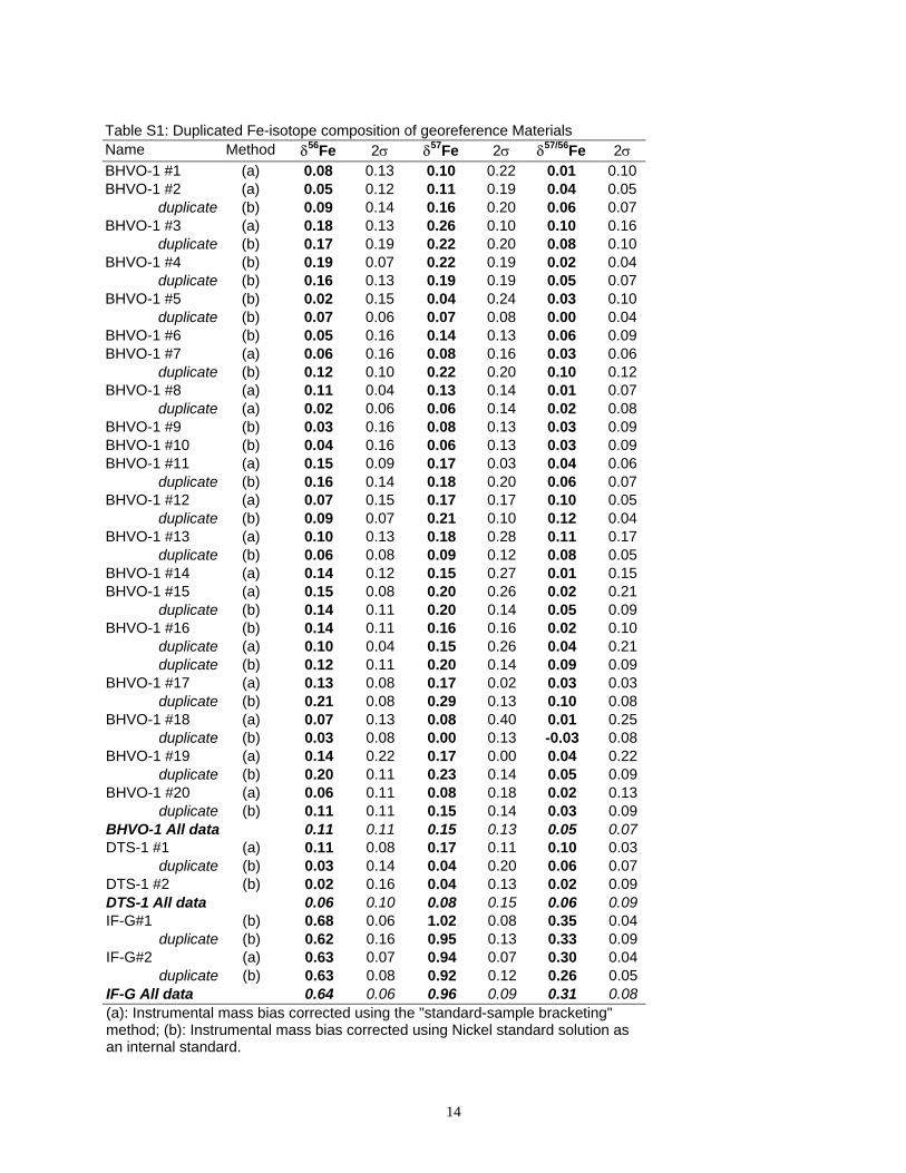
Several georeference materials (S6), including one banded iron formation (IF-G),
Hawaiian Basalt (BHVO-1) and Cr-rich ultramafic rock (DTS-1) were measured and results are
given in Table S1. Based on duplicated chemical purification and isotope analysis, the long term
external reproducibility is 0.10‰ for δ56Fe values, 0.14‰ for δ57Fe, and 0.07‰ for δ56/57Fe (2
standard deviations). Results for mantle-derived rocks give δ56Fe values between 0.07‰ to
0.11‰ relative to IRMM-14 that is statistically indistinguishable from previous studies (S4, S5).
IF-G gave δ56Fe value of 0.64‰ similar, within uncertainty, to the 0.67‰ value obtained by
Dauphas et al. (S7). Fe isotope composition of samples are given in Table S2 (Black Shales) and
Table S3 (Iron Formations) including numerous duplicate analysis which confirm the overall
4
analytical precision given above. For all samples, Fe isotope compositions determined using the
standard-sample bracketing method and using Ni as internal standard agree well within the
uncertainty (Table S1, S2 and S3) confirming further the lack of matrix effects. When Ni was
used as internal standard, Cr was not monitored during Fe isotope measurements. However, the
analysis of Cr-rich samples (DTS-1) and measurement of Cr concentration similar to the
instrumental background for selected samples together with the good relationship between
57Fe/56Fe vs. 56Fe/54Fe (see below) suggest that Cr is entirely separated from Fe during chemical
purification.
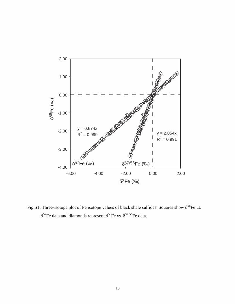
The relationships between δ56Fe, δ57Fe and δ56/57Fe for the samples analyzed in this work
are presented in Fig.S1 and all Fe-isotope values plot on a single mass fractionation line. The
slope of 0.674 ± 0.007 derived from the relationship between δ56Fe and δ57Fe (Fig. S1) is
statistically indistinguishable from that expected for equilibrium (0.678) and kinetic (0.672)
fractionations and does not permit to attribute any specific mechanism of isotope fractionation as
suggested previously (S2, S8).
2. Description of the studied material
Pyrite grains in organic-rich shales and Fe-oxides in BIFs have been selected for this
study. Pyrite occurs as nodules, disseminated grains, and laminated seams up to several
centimeters in thickness. In general, pyrite nodules are 250 µm to several cm in diameter with
variable amounts of C-rich inclusions. They either have no internal structure or are composed of
concentrically laminated, fine-grained pyrite or bladed pyrite crystals. The outer part of the
nodules is commonly overgrown by euhedral pyrite crystals. Early diagenetic origin for most
pyrite is supported by the occurrence of laminae in the shale bending around nodules. Pyrite
5
nodules often display complex features such as multiple-growth bands or composite nodules
formed by coalescence of several nodules. Dissolution and reprecipitation of primary sulfide
nodules could have happened in some samples and likely resulted in formation of massive pyrite
patches, up to several cm in thickness, often characterized by euhedral grains free of C-rich
inclusions. Short description of each sulfide sample is given in the Table S2. Geological setting
and age constraints are summarized below.
2.1. Proterozoic samples
a) ca. 1.47 Ga Newland Formation, the lower Belt Supergroup, Horse Prairie area,
Montana, USA
The minimum age for this formation is constrained by the 1469 ± 2.5 Ma and 1457 ± 2
Ma zircon ages of younger mafic sills (S9). The formation, consisting of intraclast conglomerates,
silty black shales with nodular pyrites, dolomitic silts and dolomitic gray shale beds, was
deposited in deeper water environment below wave base (S10). The lower Belt Supergroup was
deposited during the rifting stage of the Belt basin. Samples in the drill core SC-93 were collected
in the lower sulfide zone of the lower part of the Newland Formation, in very thin-bedded pyritic
black shale unit composed of few beds of intraformational conglomerate.
b) ca. 1.84 Ga Maraloou Formation, southeastern Capricorn Orogen, Australia
The minimum age of the formation is constrained by the 1843 ± 10 Ma SHRIMP U-Pb
monazite age of pepperites in the contact zone with subvolcanic dolerite sills (S11). It belongs to
the Mooloogool Subgroup of the Yerrida Group and consists of up to 1 km thick sequence of
carbonaceous shale with nodules and bands of pyrite and siltstone with minor sandstone and
carbonate deposited in restricted marine to lacustrine settings of the rift basin. Rocks experienced
very low metamorphic grade. Samples were collected from the diamond drill core KDD1.
6
c) ca. 1.88 Ga Dunn Creek Slate, Iron Crystal Falls Range, MI, USA
The Dunn Creek Slate belongs to the Paint Creek River Group which has no direct age
constraints. However, the Riverton Iron Formation overlying the Dunn Creek Slate is considered
correlative with the Gunflint and Negaunee Iron formations. The latter formations produced
similar U-Pb TIMS and SHRIMP zircon ages 1878 ± 2 and 1874 ± 9 Ma, respectively (S12). The
unit was deposited in open-marine either retroarc or foredeep Animikie basin. Samples were
collected from the drill core DL-92-1 which passed the uppermost part of the Dunn Creek Slate
(Wauseca Pyritic Member) consisting of laminated graphitic pyritic slate overlying grey sericitic
slate and siltstone (S13).
d) ca. 1.82 Ga Virginia Formation, Animikie Group, Animikie Basin, Minnesota, USA
The Virginia Formation belongs to the Animikie Group, gradationally overlies the
Biwabik Iron Formation and was deposited in either retro-arc or fore-deep Animikie Basin. The
age of this unit is constrained by the 1821 ± 16 Ma U-Pb SHRIMP zircon age of the ash-bed in
the lower part of the correlative Rove Formation in the Gunflint Range that overlies the 1878 ± 2
Ma Gunflint Iron Formation (S14, S15). The Virginia Formation consists of upward-coarsening
sequence of laminated mudstone, siltstone, and fine-grained greywacke (S16). Samples of
carbonaceous mudstones with pyrite nodules were collected from the recently drilled drill hole
VHD-00-1 in the Virginia Horn area which experienced very low metamorphic grade.
e) ca. 2.1-2.0 Ga Francevillian Series, Gabon
The age of the Francevillian Series is poorly constrained by 2036 ± 79 Ma and 2099 ± 115
Ma Sm-Nd ages of clay minerals (S17) and the 1950 ± 40 Ma age of the Oklo natural fission
reactor (S18). Carbonates in the lower part of the Francevillian Series have δ13C values ranging
from +2.1 to +6.3 ‰ (S19) suggesting deposition during the final stage of the ca. 2.22-2.06 Ga
7
carbon isotope excursion (S20). The end of this carbon isotope excursion is bracketed on the
Fennoscandian Shield and elsewhere between 2.11 and 2.06 Ga. The lower FB member consists
of black shales with pyrite and was deposited in an open-marine setting. The succession
experienced only low metamorphic grade. Samples were collected from the drill core OKP that
was collared on the Okouma plateau.
f) ca. 2.1-2.0 Ga upper Zaonezhskaya Formation, lower Ludikovian Series, Karelia, Russia
The age of the Zaonezhskaya Suite is constrained by its unconformable stratigraphic
position in the Lake Onega area above carbonates of the upper Jatulian Series that carry high 13C-
enrichment typical for the ca. 2.2-2.1 Ga carbon isotope excursion (S20). The minimum age is
constrained by 1980 ± 27 Ma Sm-Nd mineral isochron age of gabbro intrusion that cuts the
overlying unit (S21). The formation experienced greenschist facies metamorphism (S22). The
Zaonezhskaya Formation consists of a 1500-m-thick sequence of basaltic tuffs, organic-rich
siltstones and mudstones, and cherts with subordinate dolostones. Samples were collected from
the drill cores 19, 159, and 5190 from various depths.
g) ca. 2.2-2.1 Ga Sengoma Argillite Formation of the Pretoria Series, Lobatse, Botswana
The Sengoma Argillite Formation has no direct geochronologic constraints, however it is
likely correlative with the Silverton Formation of the Pretoria Group in South Africa (S23). The
Silverton Formation is intruded by the 2061 ± 2 Ma Bushveld Complex (S24). The maximum age
is constrained by the underlying 2.22 Ga Hekpoort-Ongeluk volcanics, and 2316 ± 7 Ma Re-Os
isochron pyrite age for the Rooihoogte-lower Timeball Hill formations (S25). Further constrains
are provided by the overlying carbonates that are 13C-enriched. We therefore infer that the
Sengoma Argillite Formation was deposited during the 2.2-2.1 Ga carbon isotope excursion. The
Sengoma Argillite Formation is up to 700 m in thickness upward-shallowing sequence and
consists of carbonaceous argillite with pyrite, chert, siltstone, and fine-grained quartzite.
8
Argillites often have convoluted bedding and sandstone dikes. It was deposited in deep open-
marine environment and experienced greenschist facies metamorphism. Samples were collected
from the drill core STRAT 2.
h) 2.32 Ga Rooihoogte and Timeball Hill formations, Lower Pretoria Group, Transvaal
Basin, South Africa
These units were deposited in a deltaic part of the open-marine Transvaal Basin between
the second and third glacial events of the early Paleoproterozoic (S26). Their age is well-
constrained by the 2316 ± 7 Ma Re-Os isochron pyrite age (S25). The formations experienced
lower greenschist facies metamorphism and consist of four upward-shallowing cycles of black
shale with pyrite, siltstone, and sandstone. The most organic- and pyrite-rich parts of the
sequence are in the upper part of the Rooihoogte Formation and the lower part of the Timeball
Hill Formation. For description of studied pyrite see Bekker et al. (S27). Samples were collected
from the drill cores of EBA-series that were collared in the Potchefstroom area, western part of
the Transvaal Basin and from the drill core PA-13 collared in the Penge area, eastern part of the
Transvaal Basin.
2.2. Archean Samples
a) ca. 2.5 Ga Mount McRae Shale, Mount Whaleback Mine, Newman, Hamersley Basin,
Western Australia
The age of the Mount McRae Shale is bracketed by the U-Pb SHRIMP zircon age of 2561
± 8 Ma for the Crystal Rich Tuff of the Wittenoom Dolomite and by the 2479 ± 3 Ma age for the
S9 macroband of the Dales Gorge Member of the Brockman Iron Formation (S28, S29). The
Mount McRae Shale was deposited in an open-marine setting and consists of carbonaceous
pyritic shale and minor chert layers and nodules (S30). Based on the presence of graded beds of
9
massive and plane-laminated, quartz-sericitic sandstones with tabular shale clasts and erosional
bases, dolomitized limestones with floatstones and wackestones in this unit, it was interpreted as
deposited by turbidity currents (S30). Samples were collected from the drill hole DDH44 collared
near Paraburdoo (Colonial Chert Member; upper part of the Mount McRae Shale; AMG zone 50,
0560534mE, 7429955mN) and the drill hole DO299 collared in the Whaleback Mine, Newman,
Western Australia (AMG zone 50, 0722600mE, 7412900mN).
b) ca. 2.52 Ga Gamohaan Formation, Campbellrand Subgroup, Griqualand West Basin,
South Africa
The Gamahaan Formation is the uppermost unit of the Campbellrand Subgroup
immediately underlying the ca. 2465 Ma Kuruman Iron Formation. The age of the Gamohaan
Formation is well-constrained by the TIMS U-Pb zircon age for the ash bed within this unit at
2521 ± 3 Ma (S31). The formation was deposited on the open continental margin of the Kaapvaal
Craton and consists of peritidal, subtidal, and basinal siliciclastic and carbonate rocks with
various microbialite assemblages and abundant inorganic precipitates, carbonaceous shale with
pyrite nodules, tuff, chert, and chert and dolostone breccia (S32). Carbonaceous shale is
particularly abundant near the top of the formation and contains uncompacted laminated mats and
it is interpreted to be formed in deep subtidal environments (S32). Samples were collected from
the drill hole WB-98 from the Kuruman area.
c) ca. 2.6 Ga Carawine Dolomite, Hamersley Group, Hamersley Basin, Western Australia
The Carawine Dolomite is present along the northeastern edge of the Pilbara Craton in the
area separated from the main outcrop of the Hamersley Group. The age of the Carawine
Dolomite is not constrained directly by published geochronologic data, however ash bed at the
base of the Carawine Dolomite has SHRIMP U-Pb zircon age of 2.63 Ga (Bryan Krapez, pers.
com., 2004). The maximum age of the Carawine Dolomite is constrained by the SHRIMP U-Pb

10
zircon age of 2764 ± 8 Ma for the Koongaling Volcanics at the base of the underlying Fortescue
Group in this area (S33). It overlies the Lewin Shale which is considered correlative with the ca.
2.65 Ga Jeerinah Formation. The Carawine Dolomite contains large stromatolitic domes,
laminites and clastic carbonate strata, oncolites, wave ripples, roll-up structures, and locally
preserved evaporite crystal pseudomorphs, oölites, and pisolites indicating deposition in shallow-
water platform environment (S34). The Carawine Dolomite consists almost entirely of dolomite
with thin argillite partings and beds and chert nodules (Simonson et al., 1993). Samples of the
Carawine Dolomite were collected from the drill core RHDH2A.
d) ca. 2.65 Ga Lewin Shale / Jeerinah Formation, upper part of the Fortescue Group,
Hamersley Basin, Western Australia
The age of the Jeerinah Formation and correlative Lewin Shale in the eastern part of the
Pilbara Craton is bracketed by the 2629 ± 5 Ma SHRIMP U-Pb zircon age of andesitic ignimbrite
at the top of the Roy Hill Shale Member, the upper Jeerinah Formation (S28) and 2715 ± 2 Ma
and 2713 ± 3 Ma SHRIMP U-Pb zircon ages for felsic tuffs within the underlying Maddina
Basalt (S35). The ash bed with the similar age is also present at the base of the Carawine
Dolomite (B. Krapez pers. com., 2004). Arndt et al. (S33) obtained 2684 ± 6 Ma and 2690 ± 16
Ma SHRIMP U-Pb zircon ages for the andesitic ignimbrite and tuffaceous sandstone of the upper
Jeerinah Formation. The Jeerinah Formation was deposited during the transition from the rift to
drift stage in an open-marine setting and consists of upward-fining sequence of sandstone,
siltstone, shale, and carbonaceous pyritic shale with minor chert, dolomite, and mafic and felsic
volcanic and volcanoclastic rocks (S36). Samples of the Lewin Shale were collected from the
drill core RHDH2A whereas the Roy Hill Member samples were collected from the drill core
FVG-1.
11
e) ca. 2.6 Ga Lokammona Formation, Schmidtsdrif Subgroup, Griqualand West Basin,
South Africa
The age of the Schmidtsdrif Subgroup of the Ghaap Group, the Griqualand West Basin is
only constrained by the Pb-Pb zircon age of 2642 ± 3 Ma for the Vryburg Formation, which is at
the base of the subgroup (Walvaren et al., unpubl. in Nelson et al., (S28)). The unconformably
underlying Ventersdorp Supergroup provides the maximum age constraint of 2709 ± 4 Ma for the
Schmidtsdrif Subgroup SHRIMP U-Pb zircon age for the Makwassie Quartz Porphyry Formation
(S37)). The ash bed in the lower part of the conformably overlying Campbellrand Subgroup
provides minimum age constraint for the Schmidtsdrif Subgroup of 2588 ± 6 Ma (SHRIMP U-Pb
zircon age; (S38)). The Lokammona Formation forms the uppermost part of the subgroup and
was deposited in deep-water environment on the open-marine margin and consists of upward-
fining cycles of siltstone and carbonaceous argillite with minor amounts of chert and carbonate
grainstones (S39). Carbonaceous argillites contain nodular, disseminated, and partially
recrystallized pyrite. Samples were collected from the drill hole SF-1 collared in the Vryburg
area.
f) ca. 2.72 Ga Deer Lake greenstone sequence, MN, USA
The Deer Lake greenstone sequence is located in the north-central Minnesota and belongs
to the western Wawa Subprovince of the Superior Province. No direct age constraints are
available for this Archean succession, although it is considered correlative with the Soudan Belt
of the Vermillion District and its extension to Canada, the Shebandowan greenstone Belt, both of
which developed between 2.75 and 2.67 Ga (S40, S41). The sequence experienced
metamorphism of greenschist facies and consists of interlayered mafic to intermediate volcanics,
greywackes, and carbonaceous slates and argillites with pyrite nodules up to 2 cm in diameter
(S42). Samples were collected from the drill holes 26503 and 26516.
12
g) ca. 2.72 Ga Helen Iron Formation, Michipicoten Group, MacLeod and Sir James Mines,
Wawa, Ontario, Canada
The age of the Helen Iron Formation that includes sideritic stromatolites and organic-rich
shales with pyrite nodules up to 5 cm in diameter is well-constrained by the TIMS U-Pb zircon
age of felsic tuffs immediately underlying the Iron Formation at 2749 ± 2 Ma at Helen Iron
Range in Wawa (S43) whereas in Goudreau intermediate to felsic tuffs below the correlative
Morrison No. 1 Iron Formation have TIMS U-Pb zircon age 2729 ± 2 Ma (S44). The overlying
volcanics have TIMS U-Pb zircon age of 2696 ± 2 Ma (S43). Deposition of the Helen Iron
Formation took place during the hiatus between the second and third cycles of bimodal basalt-
rhyolite volcanism at 2.75 and 2.70 Ga, respectively, in island arc to mature arc setting built on
continental crust (S45). Small bioherms with complex conical stromatolites occur at the top of the
siderite ore body in the Helen Iron Formation at the MacLeod Mine (S46). Secondary pyrite and
magnetite develop along the lamina. Carbonaceous argillite with pyrite nodules occur at the top
of the Iron Formation (S47). Pyrite nodules have radial and concentric morphology. Stromatolitic
siderite was collected in the MacLeod Mine and carbonaceous argillites with pyrite nodules were
collected on the north side of the Sir James (=Eleanor) Mine, Eleanor Iron Range.
13
y = 0.674xR2 = 0.999 y = 2.054x
R2 = 0.991
-4.00
-3.00
-2.00
-1.00
0.00
1.00
2.00
-6.00 -4.00 -2.00 0.00 2.00
δ56 F
e (‰
)
δ57Fe (‰) δ57/56Fe (‰)
δXFe (‰)
Fig.S1: Three-isotope plot of Fe isotope values of black shale sulfides. Squares show δ56Fe vs.
δ57Fe data and diamonds represent δ56Fe vs. δ57/56Fe data.
14
Table S1: Duplicated Fe-isotope composition of georeference Materials
Name Method δ56Fe 2σ δ57
Fe 2σ δ57/56Fe 2σ
BHVO-1 #1 (a) 0.08 0.13 0.10 0.22 0.01 0.10
BHVO-1 #2 (a) 0.05 0.12 0.11 0.19 0.04 0.05
duplicate (b) 0.09 0.14 0.16 0.20 0.06 0.07
BHVO-1 #3 (a) 0.18 0.13 0.26 0.10 0.10 0.16
duplicate (b) 0.17 0.19 0.22 0.20 0.08 0.10
BHVO-1 #4 (b) 0.19 0.07 0.22 0.19 0.02 0.04
duplicate (b) 0.16 0.13 0.19 0.19 0.05 0.07
BHVO-1 #5 (b) 0.02 0.15 0.04 0.24 0.03 0.10
duplicate (b) 0.07 0.06 0.07 0.08 0.00 0.04
BHVO-1 #6 (b) 0.05 0.16 0.14 0.13 0.06 0.09
BHVO-1 #7 (a) 0.06 0.16 0.08 0.16 0.03 0.06
duplicate (b) 0.12 0.10 0.22 0.20 0.10 0.12
BHVO-1 #8 (a) 0.11 0.04 0.13 0.14 0.01 0.07
duplicate (a) 0.02 0.06 0.06 0.14 0.02 0.08
BHVO-1 #9 (b) 0.03 0.16 0.08 0.13 0.03 0.09
BHVO-1 #10 (b) 0.04 0.16 0.06 0.13 0.03 0.09
BHVO-1 #11 (a) 0.15 0.09 0.17 0.03 0.04 0.06
duplicate (b) 0.16 0.14 0.18 0.20 0.06 0.07
BHVO-1 #12 (a) 0.07 0.15 0.17 0.17 0.10 0.05
duplicate (b) 0.09 0.07 0.21 0.10 0.12 0.04
BHVO-1 #13 (a) 0.10 0.13 0.18 0.28 0.11 0.17
duplicate (b) 0.06 0.08 0.09 0.12 0.08 0.05
BHVO-1 #14 (a) 0.14 0.12 0.15 0.27 0.01 0.15
BHVO-1 #15 (a) 0.15 0.08 0.20 0.26 0.02 0.21
duplicate (b) 0.14 0.11 0.20 0.14 0.05 0.09
BHVO-1 #16 (b) 0.14 0.11 0.16 0.16 0.02 0.10
duplicate (a) 0.10 0.04 0.15 0.26 0.04 0.21
duplicate (b) 0.12 0.11 0.20 0.14 0.09 0.09
BHVO-1 #17 (a) 0.13 0.08 0.17 0.02 0.03 0.03
duplicate (b) 0.21 0.08 0.29 0.13 0.10 0.08
BHVO-1 #18 (a) 0.07 0.13 0.08 0.40 0.01 0.25
duplicate (b) 0.03 0.08 0.00 0.13 -0.03 0.08
BHVO-1 #19 (a) 0.14 0.22 0.17 0.00 0.04 0.22
duplicate (b) 0.20 0.11 0.23 0.14 0.05 0.09
BHVO-1 #20 (a) 0.06 0.11 0.08 0.18 0.02 0.13
duplicate (b) 0.11 0.11 0.15 0.14 0.03 0.09
BHVO-1 All data 0.11 0.11 0.15 0.13 0.05 0.07DTS-1 #1 (a) 0.11 0.08 0.17 0.11 0.10 0.03
duplicate (b) 0.03 0.14 0.04 0.20 0.06 0.07
DTS-1 #2 (b) 0.02 0.16 0.04 0.13 0.02 0.09
DTS-1 All data 0.06 0.10 0.08 0.15 0.06 0.09IF-G#1 (b) 0.68 0.06 1.02 0.08 0.35 0.04
duplicate (b) 0.62 0.16 0.95 0.13 0.33 0.09
IF-G#2 (a) 0.63 0.07 0.94 0.07 0.30 0.04
duplicate (b) 0.63 0.08 0.92 0.12 0.26 0.05
IF-G All data 0.64 0.06 0.96 0.09 0.31 0.08(a): Instrumental mass bias corrected using the "standard-sample bracketing"method; (b): Instrumental mass bias corrected using Nickel standard solution asan internal standard.

15
Table S2: Fe-isotope composition of pyrite from Black Shales
Sample Method
δ56Fe 2σ δ57
Fe 2σ δ57/56
Fe2σ org-C Description
Kentucky Black Shales, Clay City (Devonian)Clay C. 510-519 #1 (a) 0.01 0.19 -0.02 0.18 -0.02 0.05 +++ 500µm framboids PyClay C. 510-519 #2 (a) -0.04 0.07 -0.06 0.09 -0.04 0.05 + Massive Py (in veins)
duplicate (b) -0.01 0.06 0.01 0.08 -0.01 0.04
duplicate (a) -0.04 0.08 0.01 0.10 0.03 0.05
duplicate (b) -0.02 0.16 0.06 0.13 0.04 0.09
Clay C. 193-200 (a) -0.01 0.09 -0.08 0.12 -0.03 0.13 Bulk Black Shale (Leach)
Clay C. 232-238 (b) 0.09 0.08 0.08 0.12 0.03 0.05 Bulk Black Shale (Leach)
2000NAS (b) -0.02 0.13 0.02 0.19 0.02 0.07 Bulk Black Shale (Leach)
Black Shales, Egypt (Devonian)B4,202 (b) 0.12 0.13 0.20 0.19 0.09 0.07 Bulk Black Shale (Leach)
Black Shales , Egypt (Early Cretaceous, Aptian)KB40 (b) -0.20 0.13 -0.32 0.19 -0.12 0.07 Bulk Black Shale (Leach)
Black Shales , Egypt (Late Cretaceous, Campanian)Abu-2 (b) 0.01 0.08 0.01 0.12 -0.02 0.05 Bulk Black Shale (Leach)
Black Shales , Egypt (Jurassic)B2-4 (a) 0.16 0.14 0.23 0.21 0.05 0.06 Bulk Black Shale (Leach)
Kimmeridge Bay Black Shales (Late Jurassic); Mathews et al.,2004BLN-A -0.21 -0.31 Nod. Py
BLN-C -0.30 -0.45 Nod. Py
CLN-1 -0.23 -0.34 Nod. Py
ca. 1.47 Ga Newland Formation, lower Belt Supergroup, Horse Prairie area, Montana, USASC-93, 1795 (a) -0.14 0.10 -0.30 0.14 -0.04 0.03 + Massive & Fine-g Py
duplicate (b) -0.25 0.15 -0.37 0.24 -0.11 0.10
SC-93, 1802 a (a) -0.31 0.09 -0.48 0.16 -0.14 0.13 + Massive & Fine-g Py
SC-93, 1802 b (b) -0.42 0.08 -0.65 0.10 -0.21 0.04 + Massive & Fine-g Py
SC-93, 1809 a (b) -0.39 0.14 -0.62 0.20 -0.21 0.07 + Massive & Fine-g Py
SC-93, 1809 b (b) -0.53 0.06 -0.78 0.08 -0.27 0.04 + Massive & Fine-g Py
duplicate (b) -0.64 0.04 -0.98 0.06 -0.34 0.04
ca. 1.84 Ga Maraloou Formation, southeastern Capricorn Orogen, AustraliaKDD1(1), 98.75 (a) 0.31 0.09 0.48 0.08 0.17 0.04 o Massive Py along layers
duplicate (b) 0.34 0.14 0.49 0.20 0.15 0.07
duplicate (b) 0.24 0.08 0.33 0.10 0.13 0.04
KDD1(3), 148.9 (a) 0.52 0.10 0.77 0.14 0.28 0.03 o Massive Py along layers
duplicate (b) 0.50 0.08 0.73 0.08 0.25 0.04
KDD1(6), 297.15 (b) 0.62 0.09 0.88 0.19 0.26 0.04 ++ Fine-g Py in Nodules
KDD1, 273.7 (a) 0.69 0.08 1.05 0.10 0.35 0.08 +++ Massive Py in Nodules
duplicate (b) 0.62 0.09 0.92 0.19 0.29 0.04
ca. 1.82 Ga Virginia Formation, Animikie Group, Animikie Basin, Minnesota, USAVHD-001, 1625 a (a) 0.39 0.09 0.57 0.07 0.15 0.05 o Massive & Fine-g Py
duplicate (b) 0.35 0.15 0.53 0.24 0.16 0.10
VHD-001, 1625 b (b) 0.42 0.14 0.60 0.20 0.19 0.07 o Massive & Fine-g Py
VHD-001, 203.5 (b) 0.55 0.14 0.81 0.20 0.26 0.07 o Massive Py along layers
duplicate (b) 0.62 0.05 0.94 0.08 0.32 0.04

16
ca. 1.88 Ga Dunn Creek Slate, Iron Crystal Falls Range, MI, USADL-92-1, 550 (a) 1.19 0.26 1.72 0.33 0.55 0.07 o Euh Py
duplicate (b) 1.16 0.14 1.74 0.20 0.59 0.07
duplicate (a) 1.10 0.06 1.58 0.09 0.50 0.07
duplicate (b) 1.22 0.05 1.75 0.08 0.55 0.04
ca. 2.1-2.0 Ga Francevillian Series, GabonOKP, 67.6 a (b) 0.39 0.16 0.56 0.19 0.18 0.09 +++ Fine-g Py along layers
OKP, 67.6 b (b) 0.52 0.16 0.76 0.13 0.24 0.09 +++ Fine-g Py along layers
duplicate (b) 0.51 0.08 0.77 0.12 0.25 0.05
OKP, 69.98 (a) 0.77 0.24 1.19 0.37 0.45 0.17 +++ Fine-g Py along layers
duplicate (a) 0.72 0.14 1.03 0.30 0.31 0.12
duplicate (b) 0.88 0.08 1.27 0.12 0.40 0.05
OKP, 70.45 (b) 0.12 0.16 0.23 0.19 0.04 0.09 +++ Fine-g Py along layers
OKP, 70.6 (a) -0.19 0.08 -0.25 0.11 -0.09 0.03 ++ Fine-g & Massive Pyalong layers
duplicate (b) -0.15 0.14 -0.21 0.20 -0.07 0.07
duplicate (b) -0.05 0.06 -0.15 0.09 -0.06 0.05
ca. 2.1-2.0 Ga upper Zaonezhskaya Formation, lower Ludikovian Series, Karelia, Russia159/81.5 a (a) 0.62 0.10 0.85 0.12 0.27 0.02 o Euh Py
duplicate (b) 0.72 0.06 0.99 0.08 0.30 0.04
159/81.5 b (a) -0.11 0.08 -0.09 0.10 -0.02 0.03 ++ Fine-g Py
duplicate (b) -0.06 0.06 -0.07 0.08 -0.01 0.04
19/1.62 (a) 0.06 0.06 0.09 0.08 0.02 0.06 ++ Euh Py
duplicate (b) 0.03 0.06 0.02 0.08 -0.03 0.04
19/159.5 (a) -0.20 0.06 -0.32 0.08 -0.09 0.06 o Euh Py
duplicate (b) -0.12 0.06 -0.22 0.08 -0.08 0.04
5190/158 (b) 0.94 0.06 1.43 0.08 0.51 0.04 + Massive Py
duplicate (b) 1.01 0.16 1.47 0.13 0.48 0.09
5190/85 (a) -0.24 0.05 -0.26 0.08 -0.02 0.03 +++ Massive Py
duplicate (b) -0.29 0.06 -0.39 0.08 -0.11 0.04
ca. 2.2-2.1 Ga Sengoma Argillite Formation of the Pretoria Series, Lobatse, BotswanaStrata2, 138 (b) -0.32 0.14 -0.58 0.20 -0.14 0.07 o Massive Py in nodules
duplicate (b) -0.30 0.05 -0.43 0.09 -0.15 0.05
Strata2, 192.2 (a) -0.25 0.14 -0.34 0.22 -0.08 0.09 o Euh. Py
Strata2, 192.8 (a) -0.42 0.13 -0.55 0.22 -0.13 0.09 o Massive Py in nodules
duplicate (a) -0.33 0.05 -0.49 0.08 -0.17 0.02
duplicate (b) -0.30 0.05 -0.46 0.09 -0.16 0.05
Strata2, 195.0 (a) 0.27 0.05 0.39 0.08 0.10 0.03 o Euh. Py
duplicate (b) 0.28 0.06 0.43 0.08 0.14 0.04
2.32 Ga Rooihoogte and Timeball Hill formations, Lower Pretoria Group, Transvaal Basin,South AfricaTimeball Hill Fm.
EBA-1, 1052.0 (a) 0.45 0.05 0.67 0.12 0.24 0.09 + Fine-g Py
duplicate (b) 0.56 0.07 0.82 0.10 0.28 0.04
EBA-1, 1057.93 (a) 0.93 0.05 1.36 0.13 0.44 0.08 o Massive Py
duplicate (b) 1.05 0.05 1.56 0.09 0.52 0.05
EBA-1, 1160.2 (a) -1.20 0.05 -1.81 0.09 -0.62 0.04 + Massive Py
duplicate (b) -1.37 0.14 -2.06 0.20 -0.70 0.07
duplicate (a) -1.25 0.05 -1.86 0.13 -0.63 0.08
duplicate (b) -1.15 0.05 -1.69 0.09 -0.56 0.05
EBA-3, 1164.8 (a) 0.72 0.05 1.03 0.08 0.25 0.03 o Massive & Fine-g Py
duplicate (b) 0.81 0.07 1.17 0.10 0.31 0.04

17
EBA-2/30 (a) -1.73 0.05 -2.56 0.08 -0.84 0.03 o Massive Py
duplicate (b) -1.67 0.16 -2.41 0.13 -0.73 0.09
EBA-2/31 (a) -1.02 0.05 -1.54 0.08 -0.51 0.03 + Fine-g Py
duplicate (b) -0.96 0.06 -1.47 0.08 -0.51 0.04
EBA-2/32 (a) -0.86 0.05 -1.32 0.08 -0.45 0.02 + Fine-g Py
duplicate (b) -0.88 0.06 -1.32 0.08 -0.45 0.04
EBA-2/63 (a) -1.40 0.05 -2.11 0.08 -0.70 0.02 + Massive Py
duplicate (b) -1.37 0.06 -2.04 0.08 -0.68 0.04
Rooihoogte Fm.EBA-3, 1297.5 (a) -1.33 0.05 -1.89 0.12 -0.54 0.09 o Massive Py
duplicate (b) -1.36 0.07 -1.95 0.10 -0.57 0.04
EBA-2/67 (a) -1.08 0.05 -1.60 0.08 -0.53 0.02 o Massive Py
duplicate (b) -1.05 0.06 -1.51 0.08 -0.47 0.04
EBA-2/55-2 (a) -0.76 0.08 -1.24 0.10 -0.44 0.02 o Massive Py
duplicate (b) -0.68 0.06 -1.08 0.08 -0.37 0.04
EBA-2/55-3 (a) -1.12 0.13 -1.72 0.28 -0.54 0.17 o Massive Py
duplicate (b) -1.25 0.08 -1.88 0.12 -0.59 0.05
EBA-2/59 (a) -0.21 0.13 -0.29 0.18 -0.07 0.02 o Massive Py
duplicate (b) -0.26 0.08 -0.37 0.12 -0.12 0.05
EBA-2/60 (a) -1.28 0.13 -1.97 0.18 -0.68 0.02 o Massive Py
duplicate (b) -1.23 0.08 -1.91 0.12 -0.68 0.05
ca. 2.5 Ga Mount McRae Shale, Mount Whaleback Mine, Newman, Hamersley Basin, WesternAustraliaDO299, 14.2 #1 (a) -2.03 0.07 -3.01 0.20 -0.99 0.12 + Nod py (2mm)
duplicate (b) -2.06 0.04 -3.07 0.06 -1.03 0.04
DO299, 14.2 #2 (a) -2.05 0.04 -3.07 0.08 -1.00 0.04 + Nod py (4mm)
duplicate (b) -2.00 0.04 -2.97 0.06 -0.96 0.04
DO299, 14.2 #3 (a) -1.75 0.04 -2.72 0.09 -0.96 0.04 + Nod py (4mm)
duplicate (b) -1.73 0.04 -2.67 0.06 -0.94 0.04
DO299, 14.2 #4 (a) -1.54 0.28 -2.39 0.36 -0.80 0.08 + Nod py (4mm)
duplicate (a) -1.55 0.05 -2.24 0.08 -0.69 0.04
duplicate (b) -1.58 0.08 -2.29 0.12 -0.73 0.05
DO299, 14.95 #1 (a) -1.41 0.05 -2.10 0.05 -0.70 0.03 + Nod py (2mm)
duplicate (b) -1.37 0.05 -2.08 0.08 -0.72 0.05
DO299, 14.95 #2 (a) -1.65 0.05 -2.38 0.06 -0.71 0.03 + Nod py (4mm)
duplicate (b) -1.60 0.05 -2.34 0.08 -0.73 0.05
DO299, 14.95 #3 (a) -1.98 0.05 -2.89 0.06 -0.91 0.03 + Nod py (4mm)
duplicate (b) -1.89 0.05 -2.79 0.08 -0.91 0.05
DO299, 15.2 #1 (a) -1.25 0.05 -1.76 0.08 -0.52 0.06 + Nod py (3mm)
duplicate (b) -1.25 0.05 -1.78 0.08 -0.52 0.05
DO299, 15.2 #2 (a) -1.39 0.05 -2.01 0.08 -0.63 0.06 + Nod py (3mm)
duplicate (b) -1.38 0.05 -2.01 0.08 -0.63 0.05
DO299, 15.2 #3 (a) -1.63 0.06 -2.30 0.09 -0.70 0.09 + Nod py (3mm)
duplicate (b) -1.62 0.05 -2.33 0.08 -0.72 0.05
DO299, 15.2 #4 (a) -1.23 0.25 -1.78 0.17 -0.62 0.05 + Nod py (3mm)
duplicate (b) -1.15 0.07 -1.70 0.10 -0.62 0.04
DO299, 15.7 #1 (a) -1.46 0.04 -2.09 0.01 -0.68 0.09 + Nod py (2mm)
duplicate (b) -1.48 0.05 -2.16 0.08 -0.71 0.05
DO299, 15.7 #2 (a) -1.60 0.08 -2.41 0.11 -0.81 0.10 + Nod py (2mm)
duplicate (b) -1.50 0.05 -2.28 0.08 -0.78 0.05
DO299, 15.7 #3 (a) -1.51 0.05 -2.29 0.11 -0.78 0.10 ++ Nod py (2mm)
duplicate (b) -1.47 0.05 -2.25 0.08 -0.79 0.05

18
DO299, 15.7 #4 (a) -1.13 0.03 -1.73 0.12 -0.56 0.10 ++ Nod py (2mm)
duplicate (b) -1.06 0.19 -1.66 0.19 -0.59 0.10
ca. 2.5 Ga Colonial Chert Member, Mount McRae Shale, Hamersley Basin, Western AustraliaDDH44, 516.44 (a) -1.89 0.11 -2.89 0.03 -1.00 0.05 + Massive Py
duplicate (a) -1.91 0.08 -2.76 0.15 -0.87 0.13
duplicate (b) -1.87 0.05 -2.71 0.09 -0.86 0.05
ca. 2.52 Ga Gamohaan Formation, Campbellrand Subgroup, Griqualand West Basin, SouthAfricaWB98, 477.50 (a) -0.03 0.08 0.06 0.11 0.05 0.12 + Massive Py in Nodules
duplicate (b) 0.00 0.07 0.02 0.10 0.00 0.04
WB98, 477.50 #1 (a) 0.54 0.37 0.83 0.61 0.27 0.22 + Massive Py in Nodules
duplicate (b) 0.44 0.05 0.72 0.08 0.26 0.05
WB98, 477.50 #2 (a) 0.36 0.13 0.53 0.18 0.17 0.05 + Massive Py in Nodules
duplicate (b) 0.46 0.05 0.75 0.08 0.28 0.05
WB98, 477.50 #3 (a) 0.10 0.13 0.08 0.18 -0.04 0.05 + Massive Py in Nodules
duplicate (b) 0.05 0.05 0.07 0.08 0.00 0.05
WB98, 506.15 (a) -0.68 0.08 -0.93 0.11 -0.27 0.12 o Massive Py in Nodules
duplicate (b) -0.78 0.07 -1.08 0.10 -0.34 0.04
WB98, 506.15 #1 (a) -0.86 0.23 -1.27 0.24 -0.40 0.02 o Euh. Py, disseminated inrock
duplicate (b) -0.73 0.05 -1.06 0.08 -0.35 0.05
WB98, 506.15 #2 (a) -0.94 0.23 -1.42 0.24 -0.48 0.02 o Euh. Py, disseminated inrock
duplicate (b) -1.01 0.05 -1.51 0.08 -0.51 0.05
WB98, 506.15 #3 (a) -0.87 0.06 -1.26 0.13 -0.39 0.09 o Euh. Py, disseminated inrock
duplicate (b) -0.78 0.05 -1.13 0.08 -0.37 0.05
WB98, 509.10 (b) -2.41 0.07 -3.52 0.10 -1.15 0.04 o Massive Py in Nodules
WB98, 509.10 #1 (a) -2.75 0.06 -4.09 0.13 -1.33 0.09 o Nod py (2mm)
duplicate (b) -2.67 0.05 -3.97 0.08 -1.31 0.05
WB98, 509.10 #2 (a) -2.54 0.05 -3.73 0.11 -1.21 0.07 o Nod py (4mm)
duplicate (b) -2.48 0.05 -3.61 0.08 -1.15 0.05
WB98, 509.10 #3 (a) -2.51 0.05 -3.78 0.11 -1.29 0.07 o Nod py (4mm)
duplicate (b) -2.44 0.05 -3.64 0.08 -1.22 0.05
WB98, 513.60 a (b) -1.92 0.07 -2.96 0.10 -1.03 0.04 o Massive Py in Nodules
WB98, 513.60 b (b) -1.81 0.19 -2.69 0.25 -0.89 0.08 o Massive Py in Nodules
duplicate (c) -1.83 0.07 -2.77 0.11
WB98, 519.33 (a) -2.13 0.28 -3.19 0.34 -1.06 0.06 o Massive Py in Nodules
duplicate (b) -2.13 0.19 -3.20 0.25 -1.08 0.08
duplicate (c) -2.09 0.06 -3.06 0.05
WB98, 519.63 a (a) -1.28 0.28 -1.92 0.34 -0.65 0.06 o Massive Py in Nodules
duplicate (b) -1.22 0.19 -1.84 0.25 -0.63 0.08
duplicate (c) -1.22 0.12 -1.92 0.21
WB98, 519.63 b (a) -1.31 0.20 -1.89 0.32 -0.60 0.17 o Massive Py in Nodules
duplicate (b) -1.24 0.07 -1.74 0.10 -0.53 0.04
WB98, 519.63 #1 (a) -1.36 0.24 -2.04 0.41 -0.68 0.16 o Nod py (1mm)
duplicate (b) -1.39 0.06 -2.07 0.09 -0.66 0.04
WB98, 519.63 #2 (a) -1.44 0.05 -2.18 0.08 -0.75 0.02 o Nod py (1mm)
duplicate (b) -1.30 0.06 -1.92 0.09 -0.63 0.04
WB98, 519.63 #3 (a) -1.46 0.05 -2.22 0.08 -0.78 0.02 o Nod py (1mm)
duplicate (b) -1.43 0.04 -2.13 0.06 -0.71 0.04
WB98, 520.85 (a) -2.10 0.09 -3.11 0.17 -1.02 0.12 o Massive Py in Nodules

19
WB98, 520.85#1 (a) -2.19 0.05 -3.11 0.07 -1.01 0.07 o Massive Py in Nodules
duplicate (b) -2.20 0.15 -3.20 0.24 -0.98 0.10
WB98, 520.85#2 (a) -1.98 0.05 -2.85 0.04 -0.89 0.02 o Massive Py in Nodules
duplicate (b) -2.03 0.15 -2.93 0.24 -0.92 0.10
WB98, 520.85#3 (a) -2.21 0.13 -3.29 0.18 -1.06 0.07 o Massive Py in Nodules
WB98, 522.04 (b) -2.15 0.08 -3.32 0.12 -1.13 0.05 o Massive Py in Nodules
WB98, 523.55 (a) -2.13 0.09 -3.18 0.08 -1.10 0.02 o Fine-g Py in nodules
duplicate (b) -2.24 0.15 -3.32 0.24 -1.11 0.10
ca. 2.6 Ga Carawine Dolomite, Hamersley Group, Hamersley Basin, Western AustraliaRH2A-57, 148 (a) -3.51 0.06 -5.18 0.09 -1.68 0.04 o Massive Py
duplicate (b) -3.39 0.08 -4.97 0.12 -1.60 0.05
ca. 2.6 Ga Lokammona Formation, Schmidtsdrif Subgroup, Griqualand West Basin, SouthAfricaSF-1, 599.8#1 (b) -3.27 0.13 -4.92 0.19 -1.63 0.07 o Massive Py in Nodules
duplicate (a) -3.42 0.08 -5.08 0.13 -1.64 0.11
duplicate (b) -3.39 0.06 -5.02 0.08 -1.60 0.04
SF-1, 599.8#2 (b) -3.32 0.13 -4.87 0.19 -1.58 0.07 o Massive Py in Nodules
duplicate (a) -3.38 0.08 -5.09 0.13 -1.70 0.11
duplicate (b) -3.21 0.06 -4.82 0.08 -1.59 0.04
SF-1, 611.50 (a) -2.96 0.18 -4.38 0.39 -1.42 0.21 + Massive Py in Nodules
duplicate (b) -2.98 0.19 -4.37 0.25 -1.40 0.08
duplicate (c) -2.90 0.08 -4.34 0.12
SF-1, 611.50 #1 (a) -3.04 0.08 -4.50 0.10 -1.48 0.02 + Nod py (1mm)
duplicate (b) -2.93 0.06 -4.36 0.09 -1.43 0.04
SF-1, 611.50 #2 (a) -2.90 0.08 -4.31 0.10 -1.40 0.02 + Nod py (1mm)
duplicate (b) -2.87 0.04 -4.30 0.06 -1.40 0.04
SF-1, 611.75 (a) -2.04 0.05 -3.04 0.08 -1.01 0.02 +++ Massive Py in Nodules
duplicate (b) -2.02 0.07 -3.01 0.10 -1.00 0.04
SF-1, 623.6 (a) -3.05 0.05 -4.54 0.08 -1.50 0.03 o Fine-g & Massive Py innodules
duplicate (b) -2.96 0.07 -4.40 0.10 -1.44 0.04
SF-1, 623.6 #1 (a) -2.86 0.05 -4.24 0.08 -1.34 0.02 o Massive Py in Nodules
duplicate (b) -2.77 0.06 -4.13 0.09 -1.33 0.04
SF-1, 623.6 #2 (a) -2.80 0.05 -4.13 0.08 -1.33 0.02 o Massive Py in Nodules
duplicate (b) -2.79 0.04 -4.15 0.06 -1.37 0.04
SF-1, 642.8 (a) -0.07 0.14 -0.06 0.17 0.04 0.05 +++ Massive Py in Nodules
duplicate (b) -0.19 0.07 -0.22 0.10 0.00 0.04
SF-1, 642.8 #1 (a) 0.05 0.06 0.01 0.09 -0.02 0.04 + Euh py
duplicate (b) 0.10 0.04 0.06 0.06 -0.02 0.04
SF-1, 642.8 #2 (a) -0.04 0.05 0.00 0.08 0.04 0.04 + Euh py
duplicate (b) 0.00 0.06 0.03 0.09 0.03 0.04
SF-1, 2114.2 (a) 0.06 0.14 0.10 0.17 0.08 0.05 +++ Fine-g Py
duplicate (b) 0.15 0.07 0.24 0.10 0.13 0.04
duplicate (b) 0.13 0.08 0.24 0.12 0.12 0.05
SF-1, 2175.5 (a) 0.22 0.05 0.31 0.08 0.14 0.02 ++ Fine-g Py
duplicate (b) 0.21 0.07 0.29 0.10 0.13 0.04
duplicate (a) 0.13 0.09 0.22 0.15 0.08 0.07
duplicate (b) 0.22 0.08 0.33 0.12 0.10 0.05
ca. 2.65 Ga Lewin Shale / Jeerinah Formation, Upper part of the Fortescue Group, HamersleyBasin, Western AustraliaRHDH 2A, 280.26 (a) -0.82 0.14 -1.12 0.14 -0.32 0.05 o Massive Py
duplicate (b) -0.69 0.06 -0.92 0.08 -0.24 0.04

20
2.63 Ga Roy Hill Shale Member of the Jeerinah Formation, Upper part of the FortescueGroup, Hamersley Basin, Western AustraliaFVG-1, 707.95 (b) -1.27 0.33 -1.91 0.43 -0.53 0.08 + Fine-g Py in nodules
duplicate (b) -1.26 0.19 -1.87 0.20 -0.62 0.10
FVG-1, 707.95 #1 (a) -1.68 0.05 -2.49 0.09 -0.80 0.09 + Nod py (~cm)
duplicate (b) -1.69 0.05 -2.49 0.08 -0.80 0.05
FVG-1, 707.95 #2 (a) -1.41 0.05 -2.14 0.09 -0.72 0.09 + Nod py (~cm)
duplicate (b) -1.42 0.05 -2.15 0.08 -0.72 0.05
FVG-1, 722.6 #1 (a) -1.94 0.06 -2.84 0.09 -0.92 0.02 ++ Massive Py in Nodules
duplicate (b) -1.93 0.05 -2.77 0.08 -0.87 0.05
FVG-1, 722.6 #2 (a) -1.94 0.08 -2.97 0.10 -1.03 0.04 ++ Massive Py in Nodules
duplicate (b) -2.02 0.05 -3.04 0.08 -1.03 0.05
FVG-1, 751.77 (a) -2.36 0.10 -3.58 0.12 -1.22 0.03 ++ Massive Py in Nodules
duplicate (b) -2.45 0.19 -3.73 0.25 -1.28 0.08
duplicate (c) -2.34 0.09 -3.56 0.09 Hand-picked pyritenodules
FVG-1, 752.8 (a) -2.78 0.06 -4.11 0.18 -1.32 0.12 + Massive Py in Nodules
duplicate (b) -2.72 0.07 -4.01 0.10 -1.30 0.04
FVG-1, 752.8 #1 (a) -3.06 0.07 -4.54 0.03 -1.47 0.10 + Nod py (~cm)
duplicate (b) -3.08 0.06 -4.58 0.09 -1.48 0.04
FVG-1, 752.8 #2 (a) -2.58 0.07 -3.86 0.09 -1.26 0.10 + Nod py (~cm)
duplicate (b) -2.55 0.06 -3.84 0.09 -1.26 0.04
FVG-1, 761.8 (a) -1.09 0.05 -1.89 0.08 -0.73 0.05 o Massive Py in Nodules
duplicate (b) -1.13 0.19 -1.85 0.20 -0.71 0.10
FVG-1, 761.8 #1 (a) -1.17 0.05 -1.70 0.15 -0.52 0.10 o Euh py
duplicate (b) -1.11 0.06 -1.65 0.09 -0.53 0.04
FVG-1, 761.8 #2 (a) -1.22 0.05 -1.74 0.15 -0.53 0.10 o Euh py
duplicate (b) -1.14 0.06 -1.66 0.09 -0.53 0.04
FVG-1, 777.8 (a) -1.37 0.19 -1.91 0.22 -0.53 0.05 o Euh py in nodules
duplicate (b) -1.38 0.07 -1.95 0.10 -0.56 0.04
FVG-1, 781.80 a (a) -1.91 0.19 -2.74 0.22 -0.88 0.00 o Euh py in nodules
duplicate (b) -1.92 0.07 -2.78 0.10 -0.90 0.04
FVG-1, 781.80 b (a) -2.08 0.18 -3.08 0.39 -1.01 0.21 o Euh py in nodules
duplicate (b) -2.14 0.19 -3.13 0.25 -1.00 0.08
duplicate (c) -2.10 0.07 -3.12 0.11
FVG-1, 784.1 (a) -1.74 0.09 -2.52 0.17 -0.77 0.10 + Euh py in nodules
duplicate (b) -1.80 0.16 -2.63 0.13 -0.83 0.09
FVG-1, 787.4 (a) -1.50 0.06 -2.11 0.01 -0.75 0.10 + Massive Py in nodules
duplicate (a) -1.45 0.33 -2.22 0.12 -0.71 0.18
FVG-1, 791.55 (a) -1.15 0.09 -1.61 0.11 -0.48 0.13 + Euh py in nodules
duplicate (b) -1.09 0.07 -1.51 0.10 -0.42 0.04
FVG-1, 799.0 #1 (a) -0.20 0.06 -0.34 0.09 -0.13 0.02 + Massive Py in nodules
duplicate (b) -0.17 0.06 -0.28 0.09 -0.10 0.04
FVG-1, 799.0 #2 (a) -0.76 0.05 -1.21 0.08 -0.44 0.02 + Massive Py in nodules
duplicate (b) -0.74 0.06 -1.18 0.09 -0.42 0.04
FVG-1, 814.75 (a) -1.73 0.05 -2.66 0.08 -0.89 0.12 o Euh py in nodules
duplicate (b) -1.62 0.07 -2.47 0.10 -0.81 0.04
FVG-1, 815.9 (a) -1.56 0.08 -2.35 0.10 -0.81 0.12 o Massive & Fine-g Py innodules
duplicate (b) -1.42 0.33 -2.10 0.43 -0.66 0.08
FVG-1, 826.55 (a) -1.48 0.05 -2.17 0.08 -0.67 0.12 o Massive & Euh Py innodules

21
duplicate (b) -1.48 0.07 -2.13 0.10 -0.64 0.04
FVG-1, 830.6 (a) -1.28 0.25 -1.76 0.33 -0.51 0.13 ++ Fine-g Py in nodules
duplicate (b) -1.33 0.19 -1.94 0.20 -0.60 0.10
FVG-1, 830.6 #1 (a) -1.70 0.06 -2.51 0.09 -0.82 0.02 ++ Nod py (~cm)
duplicate (b) -1.62 0.06 -2.38 0.09 -0.77 0.04
FVG-1, 830.6 #2 (a) -1.87 0.05 -2.82 0.08 -0.95 0.02 ++ Nod py (~cm)
duplicate (b) -1.90 0.04 -2.86 0.06 -0.96 0.04
FVG-1, 835.55 (a) -1.66 0.07 -2.36 0.11 -0.69 0.02 o Massive & Euh Py innodules
duplicate (b) -1.74 0.07 -2.48 0.10 -0.74 0.04
FVG-1, 849.6 (b) -0.55 0.07 -0.89 0.10 -0.33 0.04 o Massive & Fine-g Py innodules
duplicate (b) -0.62 0.19 -1.00 0.19 -0.36 0.10
FVG-1, 849.6 #1 (a) -0.95 0.05 -1.40 0.13 -0.44 0.10 o Euh py in nodules
duplicate (b) -0.97 0.05 -1.46 0.06 -0.47 0.04
FVG-1, 849.6 #2 (a) -0.87 0.08 -1.26 0.13 -0.40 0.10 o Euh py in nodules
duplicate (b) -0.90 0.05 -1.33 0.06 -0.44 0.04
ca. 2.72 Ga Helen Iron Formation, Michipicoten Group, Sir James Mines, Wawa, ON, CanadaWW1 (b) -1.76 0.16 -2.64 0.13 -0.88 0.09 nodular Py
ca. 2.72 Ga Deer Lake greenstone sequence, MN, USA#26503, 1000’ (a) -1.42 0.11 -2.02 0.12 -0.64 0.02 o Massive Py
duplicate (b) -1.31 0.15 -1.82 0.24 -0.55 0.10
#26503, 1095’ (a) -1.93 0.07 -2.91 0.11 -0.98 0.00 o Massive & Euh Py
duplicate (b) -1.85 0.07 -2.78 0.10 -0.95 0.04
#26503, 1117’ (a) -1.90 0.10 -2.79 0.20 -0.90 0.11 o Massive Py
#26516, 366’ (b) -1.94 0.15 -2.93 0.24 -1.01 0.10 o Massive Py
duplicate (b) -1.87 0.06 -2.87 0.08 -0.99 0.04
#26516, 378’ (a) -1.43 0.08 -2.26 0.11 -0.84 0.13 o Massive & Euh Py
duplicate (b) -1.37 0.07 -2.14 0.10 -0.78 0.04
(a): Instrumental mass bias corrected using the "standard-sample bracketing" method; (b):Instrumental mass bias corrected using Nickel standard solution as an internal standard (c) analysisperformed on the Nu plasma MC-ICPMS at the University of Cambridge. Sample descripton: Py:pyrite; Fine-g: fine grained crystals; Euh.: euhedral minerals: Nod: nodules (round shape andconcentric banding). Org. C: visual estimate of organic carbon content associated with pyrite grains:(o) no org. C (+) trace org. C (++) minor org. C (<1%) (+++) major org. C (<10%).
22
Table S3: Fe-isotope composition of Iron Formations
Sample Method
δ56Fe 2σ δ57
Fe 2σ δ57/56
Fe2σ Description
Upper Cherty Member, ca. 1.88 Ga Biwabik Iron Formation, Cliffs Erie Mine, Mesabi Range, MN,USABiwabik #hem (a) -0.07 0.05 -0.04 0.08 0.04 0.02 Massive Hem within silica matrix
duplicate (b) -0.07 0.16 0.01 0.13 0.02 0.09
Biwabik #mag (b) -0.23 0.08 -0.31 0.12 -0.09 0.05 Massive Mag within silica matrix
duplicate (b) -0.24 0.16 -0.38 0.13 -0.11 0.09
ca. 1.88 Ga Ironwood Iron Formation, Tyler Forks River, WI, USA4TyF-10 #mag (a) 0.48 0.17 0.58 0.29 0.13 0.10 Massive Mag within silica matrix
duplicate (b) 0.45 0.06 0.57 0.08 0.13 0.04
ca. 2.47 Ga Kuruman Iron Formation, Kuruman area, Griqualand West Basin, South AfricaKU-9-537 #mag (a) 0.46 0.05 0.77 0.08 0.26 0.02 Massive Mag within silica matrix
duplicate (b) 0.45 0.08 0.77 0.12 0.27 0.05
duplicate (b) 0.37 0.16 0.57 0.13 0.17 0.09
ca. 2.47 Ga Brockman Iron Formation, Wittenoom Gorge, Western AustraliaWIT-15 #mag (a) 0.65 0.08 0.99 0.08 0.33 0.04 Very Fine-g Mag
duplicate (b) 0.62 0.08 0.93 0.12 0.30 0.05
WIT-46 #mag (b) 0.25 0.08 0.41 0.12 0.15 0.05 Very Fine-g Mag
ca. 2.7 Ga Manjeri Formation, Belingwe Belt, Zimbabwe (Rouxel, Bickle & Galy, unpub data)MHZ 7b (c) 1.02 0.08 1.48 0.03 n.d. Fe-oxides (magnetite; hematite)
MHZ 7e (c) 1.06 0.13 1.52 0.05 n.d. Fe-oxides (magnetite; hematite)
TR 40 (c) 1.18 0.06 1.68 0.09 n.d. Fe-oxides (magnetite; hematite)
TR 42 (c) 1.16 0.13 1.70 0.18 n.d. Fe-oxides (magnetite; hematite)
TR 43 (c) 1.61 0.13 2.47 0.13 n.d. Fe-oxides (magnetite; hematite)
ca. 2.72 Ga Helen Iron Formation, Michipicoten Group, MacLeod Mine, Wawa, Ontario, CanadaStromato-carb (b) -1.28 0.06 -1.90 0.08 -0.60 0.04 honey-colored carbonate
duplicate (b) -1.33 0.16 -1.96 0.13 -0.65 0.09
Stromato-mag (b) -0.75 0.06 -1.05 0.08 -0.31 0.04 Fine-g Euh mag
duplicate (a) -0.71 0.20 -1.09 0.43 -0.37 0.22
duplicate (b) -0.71 0.16 -1.07 0.13 -0.38 0.09
Stromato-py (a) -0.91 0.09 -1.35 0.20 -0.41 0.13 Euhedral Py crystals
duplicate (b) -1.01 0.06 -1.53 0.08 -0.52 0.04
(a): Instrumental mass bias corrected using the "standard-sample bracketing" method; (b):Instrumental mass bias corrected using Nickel standard solution as an internal standard (c) analysisperformed on the Nu plasma MC-ICPMS at the University of Cambridge. Hem: hematite; Mag:magnetite; stromato: stromatolite facies composed mainly of Fe-rich carbonate (carb), disseminatedfine grained magnetite and euhedral pyrite. Fine-g: fine grained crystals; Euh.: euhedral minerals.
23
References
S1. S. Weyer, J. B. Schwieters, Int. J. Mass Spectrom. 226, 355 (2003).
S2. D. Malinovski, et al., J. Anal. Atom. Spectrom. 18, 687 (2003).
S3. N. S. Belshaw, X. K. Zhu, Y. Guo, R. K. O'Nions, Int. J. Mass Spectrom 197, 191 (2000).
S4. B. L. Beard, et al., Chem. Geol. 195, 87 (2003).
S5. O. Rouxel, N. Dobbek, J. Ludden, Y. Fouquet, Chem. Geol. 202, 155 (2003).
S6. K. Govindaraju, Geostandards Newsletter (1994), vol. 18.
S7. N. Dauphas, et al., Anal. Chem. 76, 5855 (2004).
S8. E. D. Young, A. Galy, H. Nagahara, Geochim. Cosmochim. Acta 66,, 1095 (2002).
S9. J. W. Sears, K. R. Chamberlain, S. N. Buckley, Can. J. Earth Sci. 35, 467 (1998).
S10. D. L. Feeback, (1997).
S11. B. Rasmussen, I. R. Fletcher, Earth Planet.Sci. Lett. 197, 287 (2002).
S12. D. A. Schneider, M. E. Bickford, W. F. Cannon, K. J. Schulz, M. A. Hamilton, Can. J.
Earth Sci., 39, 999 (2002).
S13. H. L. James, C. E. Dutton, F. J. Pettijohn, K. L. Wier, U.S. Geol. Surv. Prof. Paper 570
(1968).
S14. P. Fralick, D. W. Davis, S. A. Kissin, Can. J. Earth Sci., 39, 1085 (2002).
S15. S. A. Kissin, D. A. Vallini, W. D. Addison, G. R. Brumpton, paper presented at the 49th
annual meeting of the institute on Lake Superior Geology, Iron Mountain, 7 to 11 May 2003.
S16. M. E. Lucente, G. B. Morey, Minnesota Geological Survey, Report of Investigations 28, 1
(1983).
S17. R. Bros, P. Stille, F. Gauthier-Lafaye, F. Weber, N. Clauer, Earth Plan. Sci. Lett. 113, 207
(1992).
S18. F. Gauthier-Lafaye, F. Weber, Precambrian Res., 120, 81 (2003).
S19. F. Gauthier-Lafaye, F. Weber, Econ. Geol. 84, 2267 (1989).
S20. J. A. Karhu, H. D. Holland, Geology 24, 867 (1996).
S21. I. S. Pukhtel, D. Z. Zhuravlev, N. A. Ashikhmina, V. S. Kulikov, V. V. Kulikova, Doklady
Akademii Nauk Rossii (in Russian) 326, 706 (1992).
S22. V. A. Melezhik, A. E. Fallick, M. M. Filippov, O. Larsen, Earth Sci. Rev. 47, 1 (1999).
24
S23. R. M. Key, The geology of the area around Gaborone and Lobatse, Kweneng, Kgatleng,
Southern and South East Districts (Geological Survey of Botswana, Gaborone, 1983).
S24. F. Walraven, Geochronology of the Rooiberg Group, Transvaal Supergroup, South Africa
(University of the Witwatersrand, Johannesburg, South Africa, 1997).
S25. J. L. Hannah, A. Bekker, H. J. Stein, R. J. Markey, H. D. Holland, Earth Planet. Sci. Lett.
in press (2004).
S26. L. L. Coetzee, Genetic stratigraphy of the Paleoproterozoic Pretoria Group in the Western
Transvaal. (MSc. Thesis, Rand Afrikaans University, 2001).
S27. A. Bekker, et al., Nature 427, 117 (2004).
S28. D. R. Nelson, A. F. Trendall, W. Altermann, Precambrian Res. 97, 165 (1999).
S29. A. F. Trendall, D. R. Nelson, J. R. deLaeter, S. W. Hassler, Aust. J. Earth Sci., 45, 137
(1998).
S30. B. Krapez, M. E. Barley, A. L. Pickard, Sedimentology 50, 979 (2003).
S31. D. Y. Sumner, S. A. Bowring, Precambrian Res., 79, 25 (1996).
S32. D. Y. Sumner, Am. J. Sci. 297, 455 (1997).
S33. N. T. Arndt, D. R. Nelson, W. Compston, A. F. Trendall, A. M. Thorne, Aust. J. Earth Sci.,
38, 261 (1991).
S34. B. M. Simonson, K. A. Schubel, S. W. Hassler, Precambrian Res., 60, 287 (1993).
S35. T. S. Blake, R. Buick, S. J. A. Brown, M. E. Barley, Precambrian Res. 133, 143 (2004).
S36. A. M. Thorne, A. F. Trendall, Geology of the Fortescue Group, Pilbara Craton (Geological
Survey of Western Australia, 2001).
S37. R. A. Armstrong, W. Compston, E. A. Retief, I. S. Williams, H. J. Welke, Precambrian
Res., 53, 243 (1991).
S38. W. Altermann, D. R. Nelson, Jour. Sed. Geol. 120, 225 (1998).
S39. N. J. Beukes, Trans. Geol. Soc. S. Afr. 82, 313 (1979).
S40. T. J. Boerboom, R. E. Zartman, Can. J. Earth Sci. 30, 2510 (1993).
S41. F. Corfu, G. M. Stott, GSA Bull. 110, 1467 (1998).
S42. E. M. Ripley, D. L. Nicol, Geochim. Cosmochim. Acta, 45, 839 (1981).
S43. A. Turek, P. E. Smith, W. R. VanSchmus, Can. J. Earth Sci. 19, 1608 (1982).
S44. A. Turek, R. P. Sage, W. R. VanSchmus, Can. J. Earth Sci. 29, 1154 (1992).
S45. P. J. Sylvester, K. Attoh, K. J. Schulz, Can. J. Earth Sci. 24, 1120 (1987).
25
S46. H. J. Hofmann, R. P. Sage, E. N. Berdusco, Econ. Geol. 86, 1023 (1991).
S47. A. M. Goodwin, H. G. Thode, C.-L. Chou, S. N. Karkhansis, Can. J. Earth Sci. 22, 72
(1985).


