Download - IOS103 OPERATING SYSTEM MEMORY MANAGEMENT
IOS103
OPERATING SYSTEMMEMORY MANAGEMENT

Objectives
At the end of the course, the student should be able to:•Define memory management;•Discuss the concept of address binding;•Define logical and physical address space;•Discuss swapping, multiple partitions, paging and segmentation.
Memory Management
• The sharing of the CPU by several processes requires that the operating system keeps several processes (including the OS itself) in main memory at the same time.
• The operating system should therefore have
algorithms for facilitating the sharing of main memory among these processes (memory management).
Memory Management
The Concept of Address Binding
• Usually, a program resides on a disk as a binary executable file. The program must then be brought into main memory before the CPU can execute it.
• Depending on the memory management scheme, the process may be moved between disk and memory during its execution. The collection of processes on the disk that are waiting to be brought into memory for execution forms the job queue or input queue.

Memory Management
The Concept of Address Binding
• The normal procedure is to select one of the processes in the input queue and to load the process into memory.
• A user process may reside in any part of the physical memory. Thus, although the address space of the computer starts at 00000, the first address of the user process does not need to be 00000.

Memory Management
Multistep processing of a user programSource
Program
Compiler orAssembler
ObjectModule
compiletime
LinkageEditor
OtherObject
Modules
LoadModule
Loader
SystemLibrary
loadtime
In-memoryBinary
MemoryImage
DynamicallyLoadedSystemLibrary
executiontime (runtime)
dynamiclinking
Memory Management
The Concept of Address Binding• Addresses in a source program are generally
symbolic (such as LOC or ALPHA). A compiler will typically bind these symbolic addresses to relocatable addresses (such as 14 bytes from the beginning of a certain module). The linker editor or loader will then bind the relocatable addresses to absolute addresses (such as 18000H). Each binding is a mapping from one address space to another.
Memory Management
The binding of instructions and data to memory address may be done at any step along the way:1. Compile Time. If it is known at compile time where the process will reside in memory, then absolute code can be generated.•For example, if it is known that a user process resides starting at location R, then the generated compiler code will start at that location and extend up from there.•If, at some later time, the starting location changes, then it will be necessary to recompile the code.
Memory Management
2. Load Time. If it is not known at compile time where the process will reside in memory, then the compiler must generate relocatable code. In this case, final binding is delayed at load time. If the starting address changes, then the OS must reload the user code to incorporate this changed value.
Memory Management
3. Execution Time. If the process can be moved during its execution from one memory segment to another, then binding must be delayed until run time. Special hardware must be available for this scheme to work. Most general-purpose operating systems use this method.
Memory Management
The Concept of Address Binding• To obtain better memory-space utilization,
dynamic loading is often used.• With dynamic loading, a routine is not loaded
until it is called. All routines are kept on disk in a relocatable load format.
• Whenever a routine is called, the relocatable linking loader is called to load the desired routine into memory and to update the program’s address tables to reflect this change.
Memory Management
The Concept of Address Binding
• The advantage of dynamic loading is that an unused routine is never loaded. This scheme is particularly useful when large amounts of code are needed to handle infrequently occurring cases, such as error routines. In this case, although the total program size may be large, the portion that is actually used (and hence actually loaded) may be much smaller.

Memory Management
Logical and Physical Address Space• An address generated by the CPU is
commonly referred to as a logical address. • An address seen by the memory unit is
commonly referred to as a physical address. • The compile-time and load-time address
binding schemes result in an environment where the logical and physical addresses are the same.
Memory Management
Logical and Physical Address Space
• However, the execution-time address-binding scheme results in an environment where the logical and physical addresses differ.
• The run-time mapping from logical to physical addresses is done by the memory management unit (MMU), which is a hardware device.
Memory Management
Logical and Physical Address Space
• The hardware support necessary for this scheme is similar to the ones discussed earlier. The base register is now the relocation register. The value in the relocation register is added to every address generated by the user process at the time it is sent to memory.
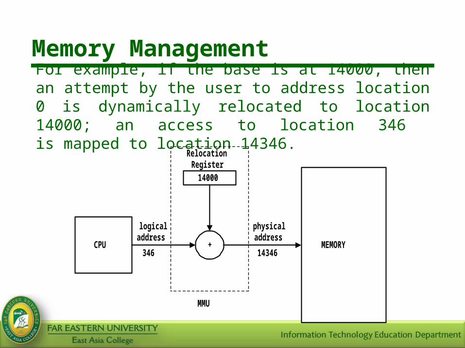
Memory ManagementFor example, if the base is at 14000, then an attempt by the user to address location 0 is dynamically relocated to location 14000; an access to location 346 is mapped to location 14346.
14000
MEMORYCPU +
RelocationRegister
logicaladdress
physicaladdress
346 14346
MMU

Memory Management
Logical and Physical Address Space
• Notice that the user program never sees the real physical addresses. The program can create a pointer to location 346, store it in memory, manipulate it, compare it to other addresses – all as the number 346. Only when it is used as a memory address is it relocated relative to the base register.

Memory Management
Logical and Physical Address Space
• There are now two different types of addresses: logical addresses (in the range 0 to max) and physical addresses (in the range R + 0 to R + max for a base value of R). The user generates only logical addresses and thinks that the process runs in locations 0 to max. The user program supplies the logical addresses; these must be mapped to physical addresses before they are used.

Memory Management
SWAPPING
• To facilitate multiprogramming, the OS can temporarily swap a process out of memory to a fast secondary storage (fixed disk) and then brought back into memory for continued execution.

Memory Management
SWAPPING
OPERATINGSYSTEM
USERSPACE
PROCESSP1
PROCESSP2
MAIN MEMORY
SECONDARY STORAGE
SWAP OUT
SWAP IN

Memory Management
SWAPPING
• For example, assume a multiprogrammed environment with a round-robin CPU-scheduling algorithm. When a quantum expires, the memory manager will start to swap out the process that just finished, and to swap in another process to the memory space that has been freed.
Memory Management
SWAPPING
• Take note that the quantum must be sufficiently large that reasonable amounts of computing are done between swaps.
• The context-switch time in swapping is fairly high.
Memory Management
Example:
Size of User Process = 1 MB= 1,048,576 bytes
Transfer Rate of Secondary Storage = 5 MB/sec
= 5,242,880 bytes/sec The actual transfer rate of the 1 MB process to or from memory takes: 1,048,576 / 5,242,880 = 200 ms
Memory Management
SWAPPING
• Assuming that no head seeks are necessary and an average latency of 8 ms, the swap time tales 208 ms. Since it is necessary to swap out and swap in, the total swap time is then about 416 ms.
Memory Management
SWAPPING
• For efficient CPU utilization, the execution time for each process must be relative long relative to the swap time. Thus, in a round-robin CPU-scheduling algorithm, for example, the time quantum should be substantially larger than 416 ms.
• Swapping is constrained by other factors as well. A process to be swapped out must be completely idle.

Memory Management
SWAPPING• Of particular concern is any pending I/O. A
process may be waiting for an I/O operation when it is desired to swap that process to free up its memory. However, if the I/O is asynchronously accessing the user memory for I/O buffers, then the process cannot be swapped.
• Assume that the I/O operation of process P1 was queued because the device was busy. Then if P1 was swapped out and process P2 was swapped in, the I/O operation might attempt to use memory that now belongs to P2.
Memory Management
SWAPPING
• Normally a process that is swapped out will be swapped back into the same memory space that it occupied previously. If binding is done at assembly or load time, then the process cannot be moved to different locations. If execution-time binding is being used, then it is possible to swap a process into a different memory space, because the physical addresses are computed during execution time.

Memory Management
MULTIPLE PARTITIONS
• In an actual multiprogrammed environment, many different processes reside in memory, and the CPU switches rapidly back and forth among these processes.
• Recall that the collection of processes on a disk that are waiting to be brought into memory for execution form the input or job queue.

Memory Management
MULTIPLE PARTITIONS
• Since the size of a typical process is much smaller than that of main memory, the operating system divides main memory into a number of partitions wherein each partition may contain exactly one process.
• The degree of multiprogramming is bounded by the number of partitions.
Memory Management
MULTIPLE PARTITIONS
• When a partition is free, the operating system selects a process from the input queue and loads it into the free partition. When the process terminates, the partition becomes available for another process.

Memory Management
MULTIPLE PARTITIONS• There are two major memory management
schemes possible in handling multiple partitions:
1. Multiple Contiguous Fixed Partition Allocation
Example: MFT Technique (Multiprogramming with a
Fixed number of Tasks) originally used by the IBM OS/360 operating system.
Memory Management
MULTIPLE PARTITIONS
• There are two major memory management schemes possible in handling multiple partitions:
2. Multiple Contiguous Variable Partition Allocation
Example: MVT Technique (Multiprogramming with a
Variable number of Tasks)
Memory Management
MULTIPLE PARTITIONS• Fixed Regions (MFT)
• In MFT, the region sizes are fixed, and do not change as the system runs.
• As jobs enter the system, they are put into a
job queue. The job scheduler takes into account the memory requirements of each job and the available regions in determining which jobs are allocated memory.
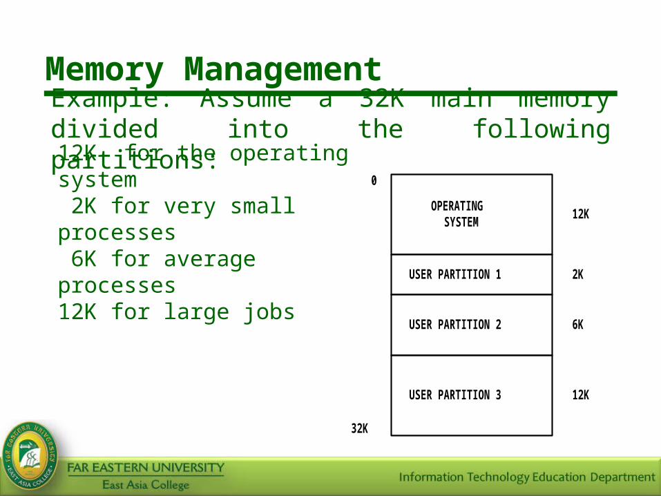
Memory ManagementExample: Assume a 32K main memory divided into the following partitions:
12K for the operating system 2K for very small processes 6K for average processes12K for large jobs
OPERATINGSYSTEM
0
32K
USER PARTITION 1
USER PARTITION 2
USER PARTITION 3
12K
2K
6K
12K
Memory Management
MULTIPLE PARTITIONS
• The operating system places jobs or process entering the memory in a job queue on a predetermined manner (such as first-come first-served).
• The job scheduler then selects a job to place in memory depending on the memory available.
Memory Management
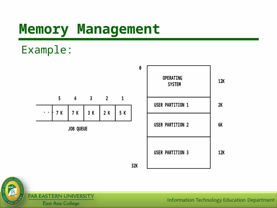
Example:
OPERATINGSYSTEM
0
32K
USER PARTITION 1
USER PARTITION 2
USER PARTITION 3
12K
2K
6K
12K
2 K3 K7 K 5 K7 K. . .
JOB QUEUE
12345
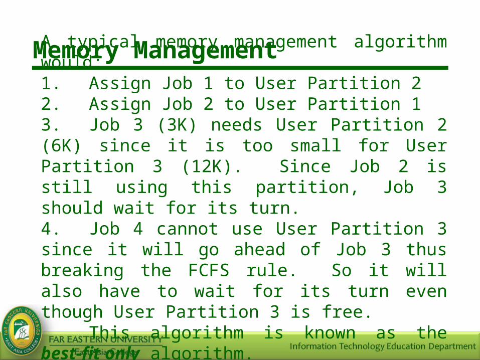
Memory ManagementA typical memory management algorithm would:1. Assign Job 1 to User Partition 22. Assign Job 2 to User Partition 13. Job 3 (3K) needs User Partition 2 (6K) since it is too small for User Partition 3 (12K). Since Job 2 is still using this partition, Job 3 should wait for its turn.4. Job 4 cannot use User Partition 3 since it will go ahead of Job 3 thus breaking the FCFS rule. So it will also have to wait for its turn even though User Partition 3 is free.
This algorithm is known as the best-fit only algorithm.

Memory Management
MULTIPLE PARTITIONS• One flaw of the best-fit only algorithm is that it
forces other jobs (particularly those at the latter part of the queue to wait even though there are some free memory partitions).
• An alternative to this algorithm is the best-fit available algorithm. This algorithm allows small jobs to use a much larger memory partition if it is the only partition left. However, the algorithm still wastes some valuable memory space.
Memory Management
MULTIPLE PARTITIONS
• Another option is to allow jobs that are near the rear of the queue to go ahead of other jobs that cannot proceed due to any mismatch in size. However, this will break the FCFS rule.

Memory Management
MULTIPLE PARTITIONSOther problems with MFT:•1. What if a process requests for more memory?
Possible Solutions:A] kill the processB] return control to the user program
with an “out of memory” messageC] reswap the process to a bigger
partition, if the system allows dynamic relocation

Memory Management
MULTIPLE PARTITIONS
• 2. How does the system determine the sizes of the partitions?
• 3. MFT results in internal and external fragmentation which are both sources of memory waste.
Memory Management
MULTIPLE PARTITIONS
• Internal fragmentation occurs when a process requiring m memory locations reside in a partition with n memory locations where m < n. The difference between n and m (n - m) is the amount of internal fragmentation.
• External fragmentation occurs when a
partition is available, but is too small for any waiting job.
Memory Management
MULTIPLE PARTITIONS
• Partition size selection affects internal and external fragmentation since if a partition is too big for a process, then internal fragmentation results. If the partition is too small, then external fragmentation occurs. Unfortunately, with a dynamic set of jobs to run, there is probably no one right partition for memory.
Memory Management
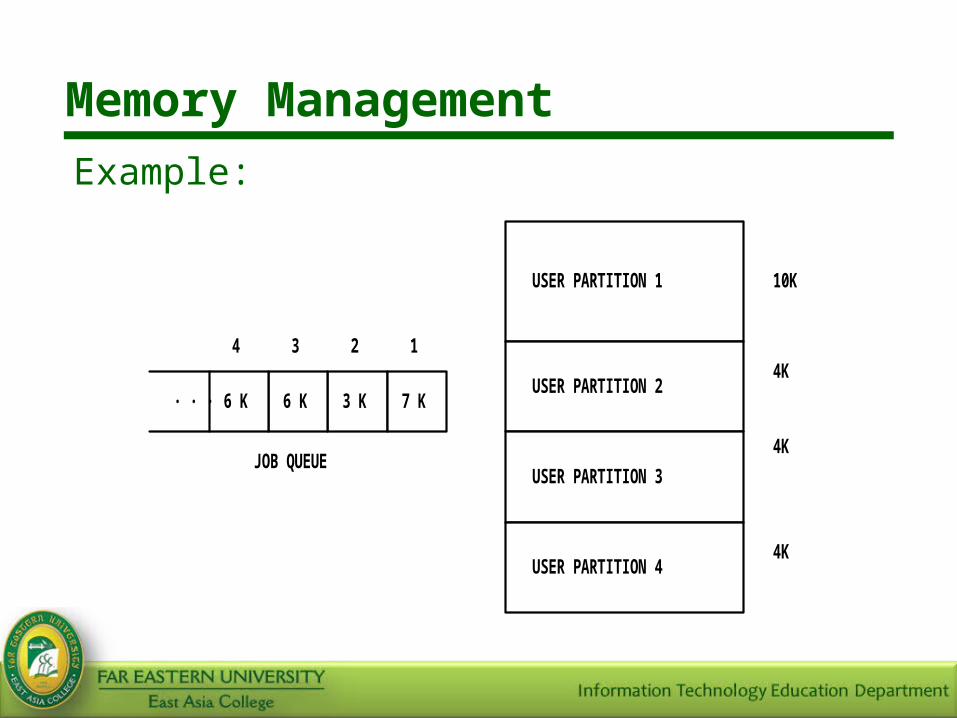
Example:
USER PARTITION 1
USER PARTITION 2
USER PARTITION 3
USER PARTITION 4
10K
4K
4K
4K
3 K6 K6 K 7 K. . .
JOB QUEUE
1234
Memory Management
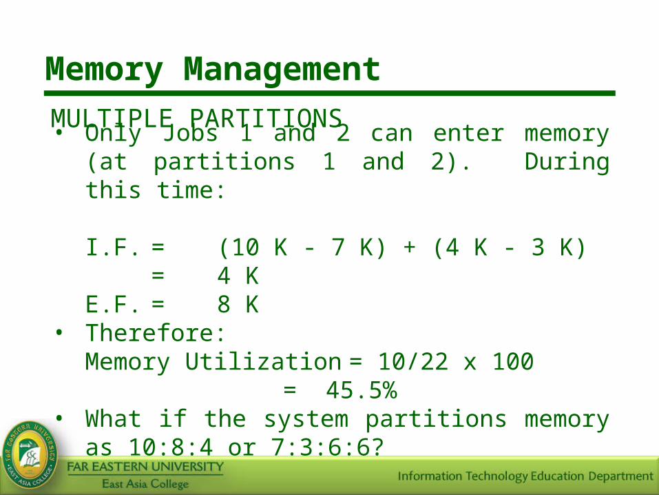
MULTIPLE PARTITIONS• Only Jobs 1 and 2 can enter memory (at
partitions 1 and 2). During this time:
I.F. = (10 K - 7 K) + (4 K - 3 K)= 4 K
E.F. = 8 K• Therefore:
Memory Utilization= 10/22 x 100= 45.5%
• What if the system partitions memory as 10:8:4 or 7:3:6:6?
Memory Management
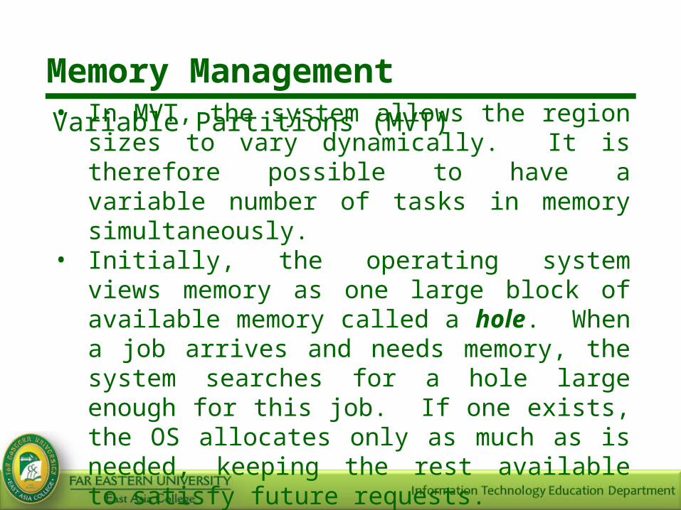
Variable Partitions (MVT)• In MVT, the system allows the region sizes to
vary dynamically. It is therefore possible to have a variable number of tasks in memory simultaneously.
• Initially, the operating system views memory as one large block of available memory called a hole. When a job arrives and needs memory, the system searches for a hole large enough for this job. If one exists, the OS allocates only as much as is needed, keeping the rest available to satisfy future requests.
Memory Management
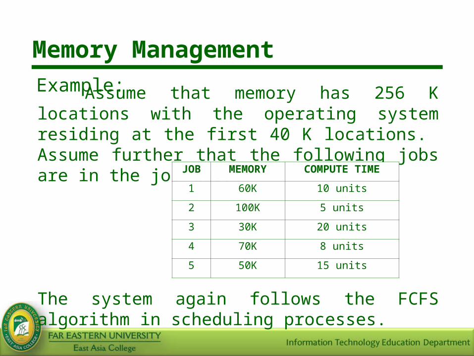
Example:Assume that memory has 256 K locations with
the operating system residing at the first 40 K locations. Assume further that the following jobs are in the job queue:
The system again follows the FCFS algorithm in scheduling processes.
JOB MEMORY COMPUTE TIME
1 60K 10 units
2 100K 5 units
3 30K 20 units
4 70K 8 units
5 50K 15 units
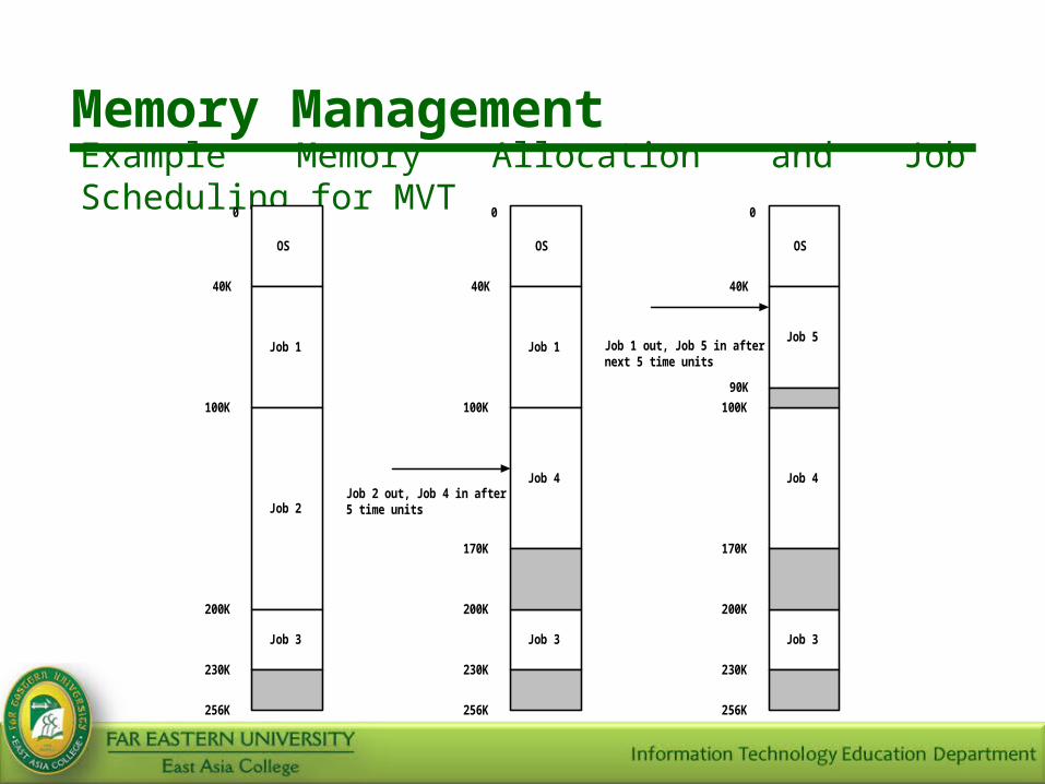
Memory ManagementExample Memory Allocation and Job Scheduling for MVT
OS
Job 1
0
Job 2
Job 3
40K
100K
200K
230K
256K
OS
Job 1
0
Job 4
Job 3
40K
100K
200K
230K
256K
170K
Job 2 out, Job 4 in after5 time units
OS
Job 5
0
Job 4
Job 3
40K
100K
200K
230K
256K
170K
Job 1 out, Job 5 in afternext 5 time units
90K
Memory Management
Variable Partitions (MVT)
• This example illustrates several points about MVT:
• 1. In general, there is at any time a set of holes, of various sizes, scattered throughout memory.
• 2. When a job arrives, the operating system searches this set for a hole large enough for the job (using the first-fit, best-fit, or worst fit algorithm).

Memory Management
Variable Partitions (MVT)
First Fit• Allocate the first hole that is large enough.
This algorithm is generally faster and empty spaces tend to migrate toward higher memory. However, it tends to exhibit external fragmentation.
Memory Management
Variable Partitions (MVT)
Best Fit• Allocate the smallest hole that is large
enough. This algorithm produces the smallest leftover hole. However, it may leave many holes that are too small to be useful.
Memory Management
Variable Partitions (MVT)
Worst Fit• Allocate the largest hole. This algorithm
produces the largest leftover hole. However, it tends to scatter the unused portions over non-contiguous areas of memory.

Memory Management
Variable Partitions (MVT)
• 3. If the hole is too large for a job, the system splits it into two: the operating system gives one part to the arriving job and it returns the other the set of holes.
• 4. When a job terminates, it releases its block of memory and the operating system returns it in the set of holes.
• 5. If the new hole is adjacent to other holes, the system merges these adjacent holes to form one larger hole.
Memory Management
Variable Partitions (MVT)
• It is important for the operating system to keep track of the unused parts of user memory or holes by maintaining a linked list. A node in this list will have the following fields:
1. the base address of the hole2. the size of the hole3. a pointer to the next node in the list

Memory Management
Variable Partitions (MVT)
• Internal fragmentation does not exist in MVT but external fragmentation is still a problem. It is possible to have several holes with sizes that are too small for any pending job.
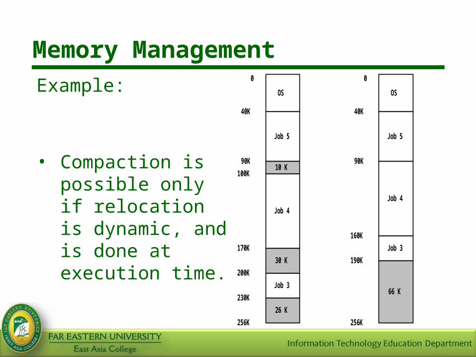
• The solution to this problem is compaction. The goal is to shuffle the memory contents to place all free memory together in one large block.
Memory Management
Example: OS
Job 5
0
Job 4
Job 3
26 K
40K
100K
200K
230K
256K
30 K
170K
10 K90K
OS
Job 5
0
Job 4
Job 3
66 K
40K
190K
256K
160K
90K• Compaction is possible only if relocation is dynamic, and is done at execution time.
Memory Management
PAGING
• MVT still suffers from external fragmentation when available memory is not contiguous, but fragmented into many scattered blocks.
• Aside from compaction, paging can minimize external fragmentation. Paging permits a program’s memory to be non-contiguous, thus allowing the operating system to allocate a program physical memory whenever possible.

Memory Management
PAGING
• In paging, the operating system divides main memory into fixed-sized blocks called frames. The system also breaks a process into blocks called pages where the size of a memory frame is equal to the size of a process page. The pages of a process may reside in different frames in main memory.
Memory Management
PAGING• Every address generated by the CPU is a
logical address. A logical address has two parts:
1. The page number (p) indicates what page the word resides.
2. The page offset (d) selects the word within the page.
Memory Management
PAGING
• The operating system translates this logical address into a physical address in main memory where the word actually resides. This translation process is possible through the use of a page table.

Memory Management
PAGING• The page number is used as an index into the
page table. The page table contains the base address of each page in physical memory.
CPU p d
logicaladdress
f
p
page table
f dMain
Memory
physicaladdress
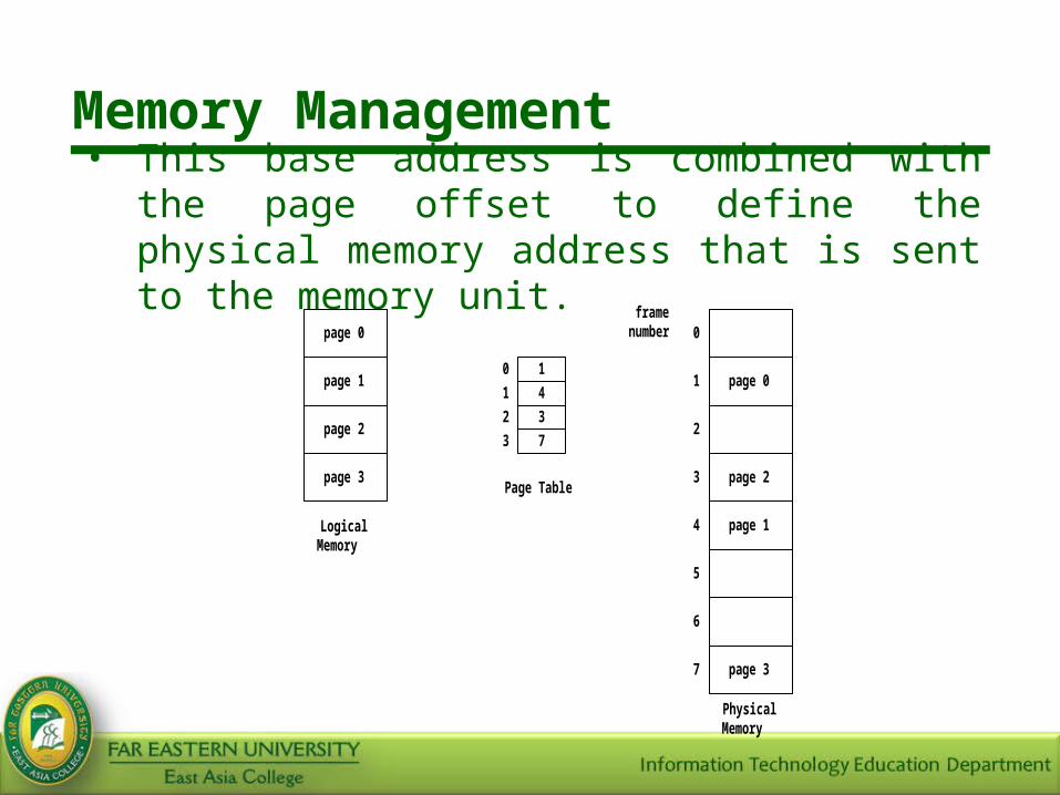
Memory Management• This base address is combined with the page
offset to define the physical memory address that is sent to the memory unit.
page 0
LogicalMemory
1page 1
page 2
page 3
4
3
7
0
1
2
3
Page Table
page 0
page 2
page 3
page 1
PhysicalMemory
0
1
2
3
4
5
6
7
framenumber
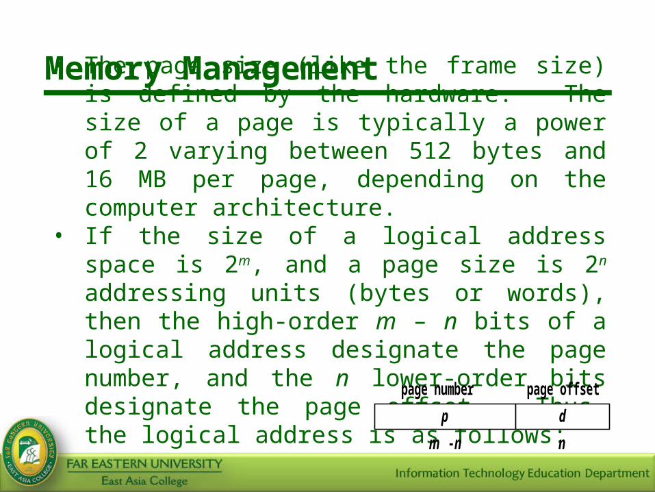
Memory Management• The page size (like the frame size) is defined by
the hardware. The size of a page is typically a power of 2 varying between 512 bytes and 16 MB per page, depending on the computer architecture.
• If the size of a logical address space is 2m, and a page size is 2n addressing units (bytes or words), then the high-order m – n bits of a logical address designate the page number, and the n lower-order bits designate the page offset. Thus, the logical address is as follows:
p d
m - n n
page number page offset
Memory Management
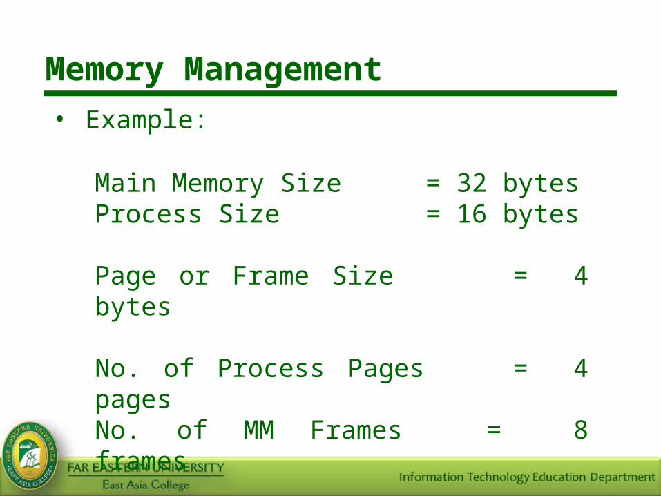
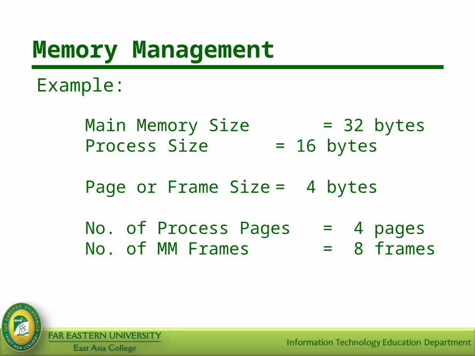
• Example:
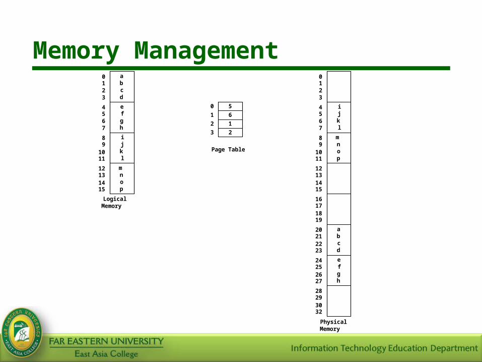
Main Memory Size = 32 bytesProcess Size = 16 bytes Page or Frame Size = 4 bytes No. of Process Pages = 4 pagesNo. of MM Frames = 8 frames
Memory Managementabcd
LogicalMemory
5
6
1
2
0
1
2
3
Page Table
PhysicalMemory
0123
efgh
4567
ijkl
89
1011
mnop
12131415
abcd
0123
efgh
4567
ijkl
89
1011
12131415
mnop
16171819
20212223
24252627
28293032

Memory Management
PAGING
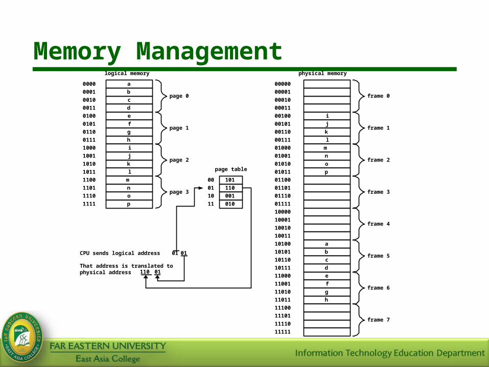
• Logical address 0 is page 0, offset 0. Indexing into the page table, it is seen that page 0 is in frame 5. Thus, logical address 0 maps to physical address 20 (5 x 4 + 0). Logical address 3 (page 0, offset 3) maps to physical address 23 (5 x 4 + 3). Logical address 4 is page 1, offset 0; according to the page table, page 1 is mapped to frame 6. Thus logical address 4 maps to physical address 24 (6 x 4 + 0). Logical address 13 maps to physical address 9.
Memory Management
Example:
Main Memory Size = 32 bytesProcess Size = 16 bytes
Page or Frame Size = 4 bytes
No. of Process Pages = 4 pagesNo. of MM Frames = 8 frames

Memory Management
Example:
Logical Address Format:
A3 A2 A1 A0
page offset
page number
Memory Management
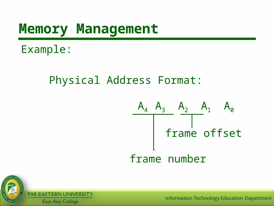
Example:
Physical Address Format:
A4 A3 A2 A1 A0
frame offset
frame number
Memory Managementa0000
b0001
c0010
d0011
page 0
e0100
f0101
g0110
h0111
page 1
i1000
j1001
k1010
l1011
page 2
m1100
n1101
o1110
p1111
page 3
logical memory physical memory
00000
00001
00010
00011
frame 0
i00100
j00101
k00110
l00111
frame 1
m01000
n01001
o01010
p01011
frame 2
01100
01101
01110
01111
frame 3
10000
10001
10010
10011
frame 4
a10100
b10101
c10110
d10111
frame 5
e11000
f11001
g11010
h11011
frame 6
11100
11101
11110
11111
frame 7
101
110
001
010
page table
00
01
10
11
CPU sends logical address
That address is translated tophysical address
01 01
110 01
Memory Management
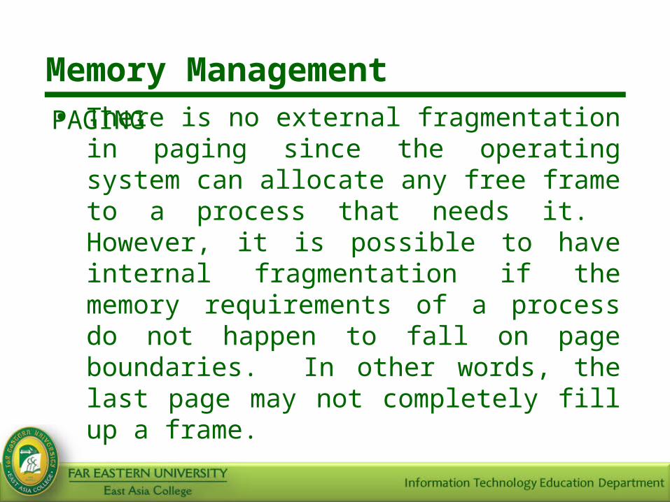
PAGING
• There is no external fragmentation in paging since the operating system can allocate any free frame to a process that needs it. However, it is possible to have internal fragmentation if the memory requirements of a process do not happen to fall on page boundaries. In other words, the last page may not completely fill up a frame.
Memory Management
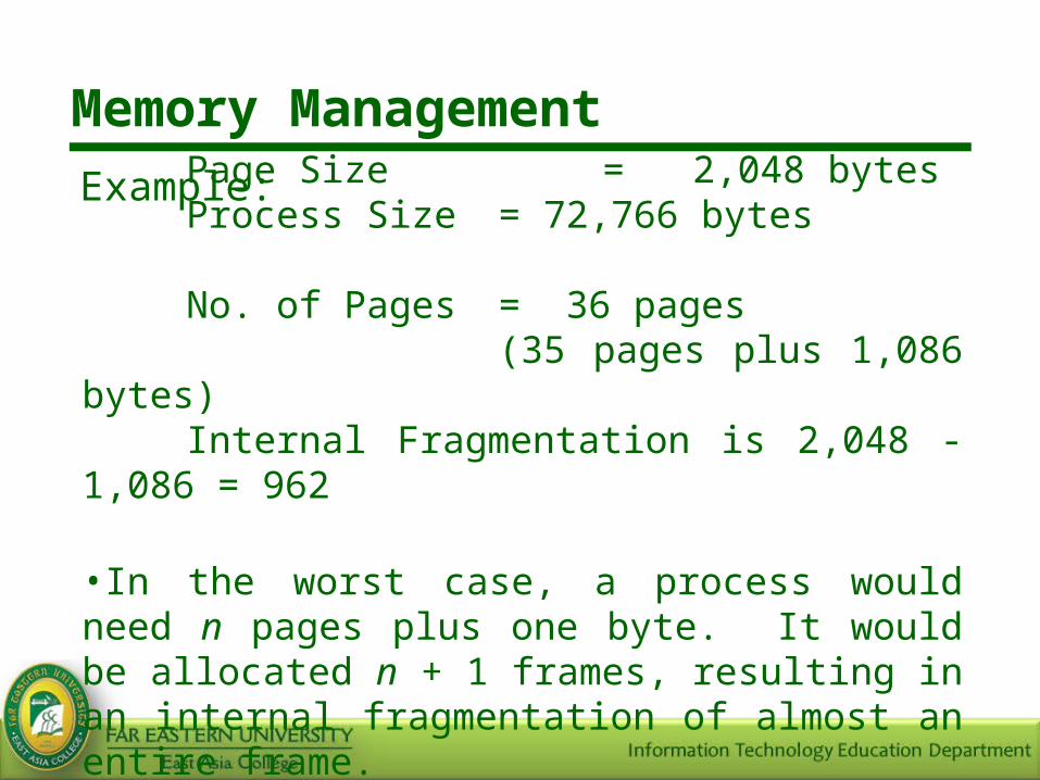
Example:Page Size = 2,048 bytesProcess Size = 72,766 bytes
No. of Pages = 36 pages
(35 pages plus 1,086 bytes) Internal Fragmentation is 2,048 - 1,086 = 962
•In the worst case, a process would need n pages plus one byte. It would be allocated n + 1 frames, resulting in an internal fragmentation of almost an entire frame.
Memory Management
PAGING
• If process size is independent of page size, it is expected that internal fragmentation to average one-half page per process. This consideration suggests that small page sizes are desirable. However, overhead is involved in each page-table entry, and this overhead is reduced as the size of the pages increases. Also, disk I/O is more efficient when the number of data being transferred is larger.

Memory Management
PAGING
• Each operating system has its own methods for storing page tables. Most allocate a page table for each process. A pointer to the page table is stored with the other register values (like the program counter) in the PCB. When the dispatcher is told to start a process, it must reload the user registers and define the correct hardware page-table values from the stored user page table.
Memory Management
• The options in implementing page tables are:
1. Page Table RegistersIn the simplest case, the page table is implemented as a set of dedicated registers. These registers should be built with high-speed logic to make page-address translation efficient. The advantage of using registers in implementing page tables is fast mapping. Its main disadvantage is that it becomes expensive for large logical address spaces (too many pages).
Memory Management
2. Page Table in Main Memory
The page table is kept in memory and a Page Table Base Register (PTBR) points to the page table. The advantage of this approach is that changing page tables requires changing only this register, substantially reducing context switch time. However, two memory accesses are needed to access a word.
Memory Management
3. Associative Registers
The standard solution is to use a special, small, fast-lookup hardware cache, variously called Associative Registers or Translation Look-aside Buffers (TLB).

Memory Management
• The associative registers contain only a few of the page-table entries. When a logical address is generated by the CPU, its page number is presented to a set of associative registers that contain page numbers and their corresponding frame numbers. If the page number is found in the associative registers, its frame number is immediately available and is used to access memory.
Memory Management
• If the page number is not in the associative registers, a memory reference to the page table must be made. When the frame number is obtained, it can be used to access memory (as desired). In addition, the page number and frame number is added to the associative registers, so that they can be found quickly on the next reference.
Memory Management• Another advantage in paging is that processes
can share pages therefore reducing overall memory consumption.Example: Consider a system that supports 40 users, each of whom executes a text editor. If the text editor consists of 150K of code and 50K of data space, then the system would need 200K x 40 = 8,000K to support the 40 users.However, if the text editor code is reentrant (pure code that is non-self-modifying), then all 40 users can share this code. The total memory consumption is therefore 150K + 50K x 40 = 2,150K only.

Memory Management
PAGING
• It is important to remember that in order to share a program, it has to be reentrant, which implies that it never changes during execution.
Memory Management
SEGMENTATION
• Because of paging, there are now two ways of viewing memory. These are the user’s view (logical memory) and the actual physical memory. There is a necessity of mapping logical addresses into physical addresses.
Memory Management
SEGMENTATION
• Logical Memory
• A user or programmer views memory as a collection of variable-sized segments, with no necessary ordering among the segments.
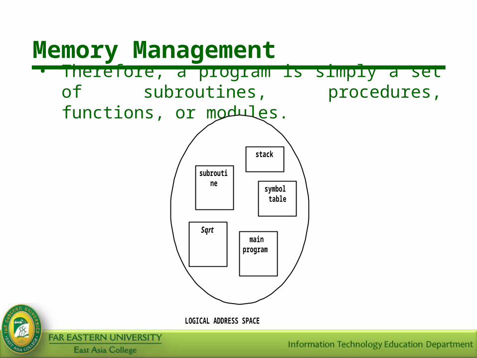
Memory Management• Therefore, a program is simply a set of
subroutines, procedures, functions, or modules.
subroutine
stack
Sqrtmain
program
symboltable
LOGICAL ADDRESS SPACE

Memory Management
SEGMENTATION
• Each of these segments is of variable-length; the size is intrinsically defined by the purpose of the segment in the program. The user is not concerned whether a particular segment is stored before or after another segment. The OS identifies elements within a segment by their offset from the beginning of the segment.

Memory Management
SEGMENTATION
Example: The Intel 8086/88 processor has four segments:
1. The Code Segment2. The Data Segment3. The Stack Segment4. The Extra Segment
Memory Management
SEGMENTATION
• Segmentation is the memory-management scheme that supports this user’s view of memory. A logical address space is a collection of segments. Each segment has a name and a length. Addresses specify the name of the segment or its base address and the offset within the segment.

Memory Management
SEGMENTATION
Example:
To access an instruction in the Code Segment of the 8086/88 processor, a program must specify the base address (the CS register) and the offset within the segment (the IP register).

Memory Management
The mapping of logical address into physical address is possible through the use of a segment table.
d < limit ?
limit
CPU (s, d)
to MMtrue
trap to operating system monitor --addressing error
false
base
s
+
Memory Management
SEGMENTATION
• A logical address consists of two parts: a segment number s, and an offset into the segment, d. The segment number is an index into the segment table. Each entry of the segment table has a segment base and a segment limit. The offset d must be between 0 and limit.
Memory Management
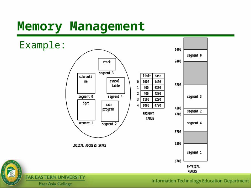
Example:
subroutine
stack
Sqrt mainprogram
symboltable
LOGICAL ADDRESS SPACE
segment 0
segment 1 segment 2
segment 3
segment 4
limit base
1000
400
400
1100
1000
1400
6300
4300
3200
4700
0
1
2
3
4
SEGMENTTABLE
segment 0
segment 3
segment 2
segment 4
segment 1
1400
2400
3200
4300
4700
5700
6300
6700
PHYSICALMEMORY
Memory Management
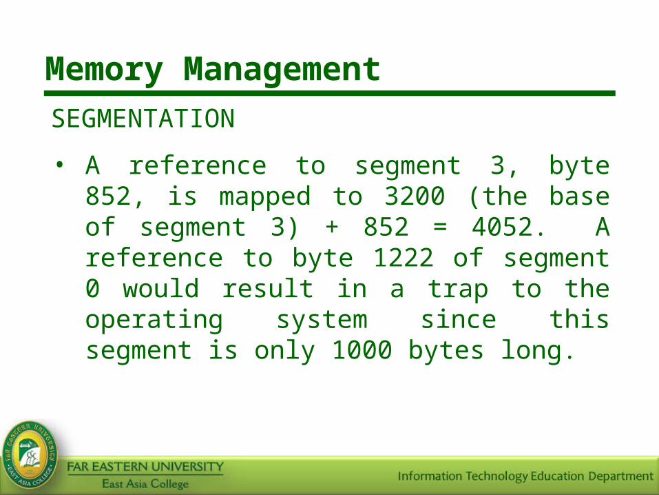
SEGMENTATION
• A reference to segment 3, byte 852, is mapped to 3200 (the base of segment 3) + 852 = 4052. A reference to byte 1222 of segment 0 would result in a trap to the operating system since this segment is only 1000 bytes long.


