
INV ITEDP A P E R
Optimal Parameters forLocality-Sensitive HashingAn algorithm is described that optimizes parameters for nearest-neighbor
retrieval in web-scale search, at minimum computational cost.
ByMalcolm Slaney, Fellow IEEE, Yury Lifshits, and Junfeng He
ABSTRACT | Locality-sensitive hashing (LSH) is the basis of
many algorithms that use a probabilistic approach to find
nearest neighbors. We describe an algorithm for optimizing the
parameters and use of LSH. Prior work ignores these issues or
suggests a search for the best parameters. We start with two
histograms: one that characterizes the distributions of dis-
tances to a point’s nearest neighbors and the second that
characterizes the distance between a query and any point in
the data set. Given a desired performance level (the chance of
finding the true nearest neighbor) and a simple computational
cost model, we return the LSH parameters that allow an LSH
index to meet the performance goal and have the minimum
computational cost. We can also use this analysis to connect
LSH to deterministic nearest-neighbor algorithms such as k-d
trees and thus start to unify the two approaches.
KEYWORDS | Database index; information retrieval; locality-
sensitive hashing; multimedia databases; nearest-neighbor
search
I . INTRODUCTION
It seems like a simple problem: Given a set of data and a
query, find the point in the data set that is nearest to the
query. One calculates the distance between the query and
each point in the database, and then returns the identity of
the closest point. This is an important problem in many
different domains, for example, query by example and
multimedia fingerprinting [10]. We can find the nearestneighbors by checking the distance to every point in the
data set, but the cost of this approach is prohibitive in all
but the smallest data sets, and completely impractical in an
interactive setting. We wish to find a solution, an index,
whose cost is very, very sublinear in the number of points
in the database.
The simplicity of the problem belies the computational
complexity when we are talking about high-dimensional,web-scale collections. Most importantly, the curse of
dimensionality [19] makes it hard to reason about the
problem. Secondarily, the difficulty of the solution is
complicated by the fact that there are two thoroughly
researched and distinct approaches to the problem:
probabilistic and deterministic. The stark difference in
approaches makes them hard to compare. Later in this
paper we will show that the two methods have much incommon and suggest a common framework for further
analysis.
The primary contribution of this paper is an algorithm
to calculate the optimum parameters for nearest-neighbor
search using a simple probabilistic approach known as
locality-sensitive hashing (LSH), which we describe in
Section II. The probabilistic nature of the data and the
algorithm means that we can derive an estimate of the costof a lookup. Cost is measured by the time it takes to
perform a lookup, including cache and disk access. Our
optimization procedure depends on the data’s distribution,
something we can compute from a sample of the data, and
the application’s performance requirements. Our approach
is simple enough that we can use it to say a few things
about the performance of deterministic indexing, and thus
start to unify the approaches.In conventional computer hashing, a set of objects (i.e.,
text strings) are inserted into a table using a function that
converts the object into pseudorandom ID called a hash.
Manuscript received July 7, 2011; revised February 8, 2012; accepted March 18, 2012.
Date of publication July 17, 2012; date of current version August 16, 2012.
M. Slaney was with Yahoo! Research, Sunnyvale, CA 94089 USA. He is now with
Microsoft in Mountain View, CA (e-mail: [email protected]).
Y. Lifshits was with Yahoo! Research, Sunnyvale, CA 94089 USA
(e-mail: [email protected]).
J. He was with Yahoo! Research, Sunnyvale, CA 94089 USA. He is now with Columbia
University, New York, NY 10027 USA (e-mail: [email protected]).
Digital Object Identifier: 10.1109/JPROC.2012.2193849
2604 Proceedings of the IEEE | Vol. 100, No. 9, September 2012 0018-9219/$31.00 �2012 IEEE
Given the object, we compute an integer-valued hash, andthen go to that location in an array to find the matches.
This converts a search problem, which implies looking at a
large number ðNÞ of different possible objects and could
take OðNÞ or OðlogðNÞÞ time, into a memory lookup with
cost that could be Oð1Þ. This is a striking example of the
power of a conventional hash.
In the problems we care about, such as finding nearest
neighbors in a multimedia data set, we do not have exactmatches. Due to the vagaries of the real world, not to
mention floating point errors, we are looking for matches
that are close to the query. A conventional hash does not
work because small differences between objects are
magnified so the symbols Bfoo[ and Bfu[ get sent to
widely differing buckets. Some audio fingerprinting work,
for example, chooses features that are robust so they can
use exact indices to perform the lookup [25]. But in thiswork we consider queries that are more naturally
expressed as a nearest-neighbor problem.
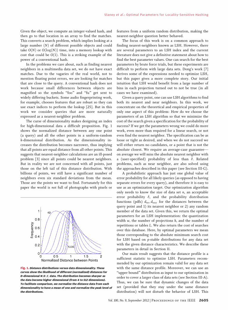
The curse of dimensionality makes designing an index
for high-dimensional data a difficult proposition. Fig. 1
shows the normalized distance between any one point
(a query) and all the other points in a uniform-random
k-dimensional distribution. As the dimensionality in-
creases the distribution becomes narrower, thus implyingthat all points are equal distance from all other points. This
suggests that nearest-neighbor calculations are an ill-posed
problem [3] since all points could be nearest neighbors.
But in reality we are not concerned with all points, justthose on the left tail of this distance distribution. With
billions of points, we still have a significant number of
neighbors even six standard deviations from the mean.
Those are the points we want to find. Fortunately for thispaper the world is not full of photographs with pixels or
features from a uniform random distribution, making thenearest-neighbor question better behaved.
The focus of this work is on a common approach to
finding nearest-neighbors known as LSH. However, there
are several parameters to an LSH index and the current
literature does not give a definitive statement about how to
find the best parameter values. One can search for the best
parameters by brute force trials, but these experiments are
difficult to perform with large data sets. Dong’s work [7]derives some of the expressions needed to optimize LSH,
but this paper gives a more complete story. Our initial
intuition that LSH would benefit from a large number of
bins in each projection turned out to not be true (in all
cases we have examined).
Given a query point, one can use LSH algorithms to find
both its nearest and near neighbors. In this work, we
concentrate on the theoretical and empirical properties ofonly one aspect of this problem: How do we choose the
parameters of an LSH algorithm so that we minimize the
cost of the search given a specification for the probability of
success? If we get the parameters wrong we could do more
work, even more than required for a linear search, or not
even find the nearest neighbor. The specification can be as
loose or tight as desired, and when we do not succeed we
will either return no candidates, or a point that is not theabsolute closest. We require an average-case guaranteeVon average we will miss the absolute nearest neighbor with
a (user-specified) probability of less than �. Related
problems, such as near neighbor, are also solved using
the approaches described in this paper (see Section III-G).
A probabilistic approach has just one global value of
error probability for all likely queries (as opposed to having
separate errors for every query), and therefore it is easy touse as an optimization target. Our optimization algorithm
only needs to know the size of data set n, an acceptable
error probability �, and the probability distribution
functions (pdfs) dnn; dany for the distances between the
query point and 1) its nearest neighbor or 2) any random
member of the data set. Given this, we return the optimal
parameters for an LSH implementation: the quantization
width w, the number of projections k, and the number ofrepetitions or tables L. We also return the cost of searches
over this database. Here, by optimal parameters we mean
those corresponding to the absolute minimum search cost
for LSH based on p-stable distributions for any data set
with the given distance characteristics. We describe these
parameters in detail in Section II.
Our main result suggests that the distance profile is a
sufficient statistic to optimize LSH. Parameters recom-mended by our optimization remain valid for any data set
with the same distance profile. Moreover, we can use an
Bupper bound[ distribution as input to our optimization in
order to cover a larger class of data sets (see Section III-A).
Thus, we can be sure that dynamic changes of the data
set (provided that they stay under the same distance
distribution) will not disturb the behavior of LSH. This
Fig. 1. Distance distributions versus data dimensionality. These
curves show the likelihood of different (normalized) distances for
D-dimensional Nð0; 1Þ data. The distribution becomes sharper as
the data become higher dimensional (from 4 to 512 dimensions).
To facilitate comparison, we normalize the distance data from each
dimensionality to have a mean of one and normalize the peak level of
the distributions.
Slaney et al. : Optimal Parameters for Locality-Sensitive Hashing
Vol. 100, No. 9, September 2012 | Proceedings of the IEEE 2605
stability property is important for practical implementa-
tions. Recommended LSH parameters are independent of
the representational dimension. Thus, if one takes a 2-Ddata set and puts it in 100-dimensional space, our
optimization algorithm will recommend the same para-
meters and provide the same search cost. This property
was not previously observed for LSH.1
This paper describes an approach to find the optimal
parameters for a nearest-neighbor search implemented
with LSH. We describe LSH and introduce our parameters
in Section II. Section III describes the parameteroptimization algorithm and various simplifications.
Section IV describes experiments we used to validate our
results. We talk about related algorithms and deterministic
variations such as k-d trees in Section V.
II . INTRODUCTION TOLOCALITY-SENSITIVE HASHING
In this work, we consider LSH based on p-stable distri-
butions as introduced by Datar et al. [6]. Following the
tutorial by Slaney and Casey [24], we analyze LSH as an
algorithm for exact nearest-neighbor search. Our tech-
nique applies to the approximate near-neighbor algorithm
as originally proposed by Datar et al. [6] and as we describein Section III-A. We only consider distances computed
using the Euclidean norm ðL2Þ. Below we present a short
summary of the algorithm.
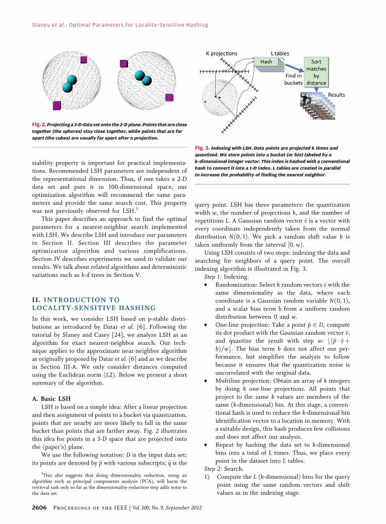
A. Basic LSHLSH is based on a simple idea: After a linear projection
and then assignment of points to a bucket via quantization,
points that are nearby are more likely to fall in the samebucket than points that are farther away. Fig. 2 illustrates
this idea for points in a 3-D space that are projected onto
the (paper’s) plane.
We use the following notation: D is the input data set;
its points are denoted by �p with various subscripts; �q is the
query point. LSH has three parameters: the quantizationwidth w, the number of projections k, and the number of
repetitions L. A Gaussian random vector �v is a vector withevery coordinate independently taken from the normal
distribution Nð0; 1Þ. We pick a random shift value b is
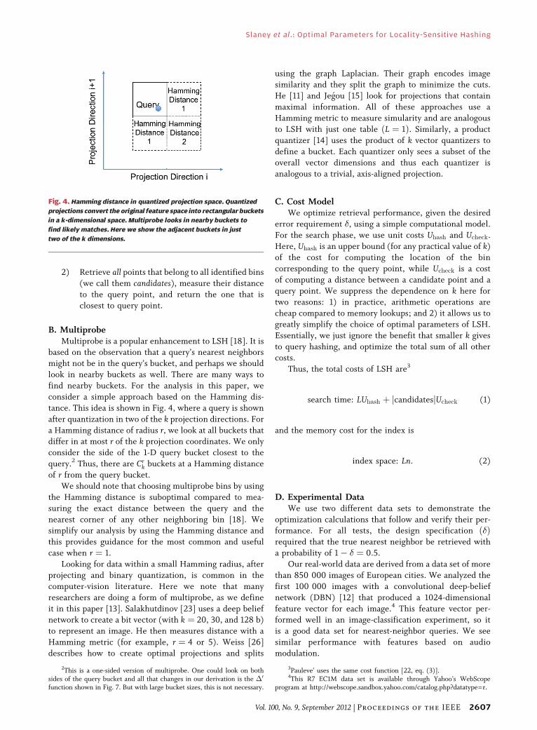
taken uniformly from the interval ½0;wÞ.Using LSH consists of two steps: indexing the data and
searching for neighbors of a query point. The overall
indexing algorithm is illustrated in Fig. 3.Step 1: Indexing.• Randomization: Select k random vectors �v with the
same dimensionality as the data, where each
coordinate is a Gaussian random variable Nð0; 1Þ,and a scalar bias term b from a uniform random
distribution between 0 and w.• One-line projection: Take a point �p 2 D, compute
its dot product with the Gaussian random vector �v,and quantize the result with step w: bð�p � �vþbÞ=wc. The bias term b does not affect our per-
formance, but simplifies the analysis to follow
because it ensures that the quantization noise is
uncorrelated with the original data.
• Multiline projection: Obtain an array of k integersby doing k one-line projections. All points that
project to the same k values are members of thesame (k-dimensional) bin. At this stage, a conven-
tional hash is used to reduce the k-dimensional bin
identification vector to a location in memory. With
a suitable design, this hash produces few collisions
and does not affect our analysis.
• Repeat by hashing the data set to k-dimensional
bins into a total of L times. Thus, we place every
point in the dataset into L tables.Step 2: Search.1) Compute the L (k-dimensional) bins for the query
point using the same random vectors and shift
values as in the indexing stage.
1This also suggests that doing dimensionality reduction, using analgorithm such as principal components analysis (PCA), will harm theretrieval task only so far as the dimensionality-reduction step adds noise tothe data set.
Fig. 2.Projectinga3-Ddatasetonto the2-Dplane.Points thatare close
together (the spheres) stay close together, while points that are far
apart (the cubes) are usually far apart after a projection.
Fig. 3. Indexing with LSH. Data points are projected k times and
quantized. We store points into a bucket (or bin) labeled by a
k-dimensional integer vector. This index is hashedwith a conventional
hash to convert it into a 1-D index. L tables are created in parallel
to increase the probability of finding the nearest neighbor.
Slaney et al.: Optimal Parameters for Locality-Sensitive Hashing
2606 Proceedings of the IEEE | Vol. 100, No. 9, September 2012
2) Retrieve all points that belong to all identified bins(we call them candidates), measure their distance
to the query point, and return the one that isclosest to query point.
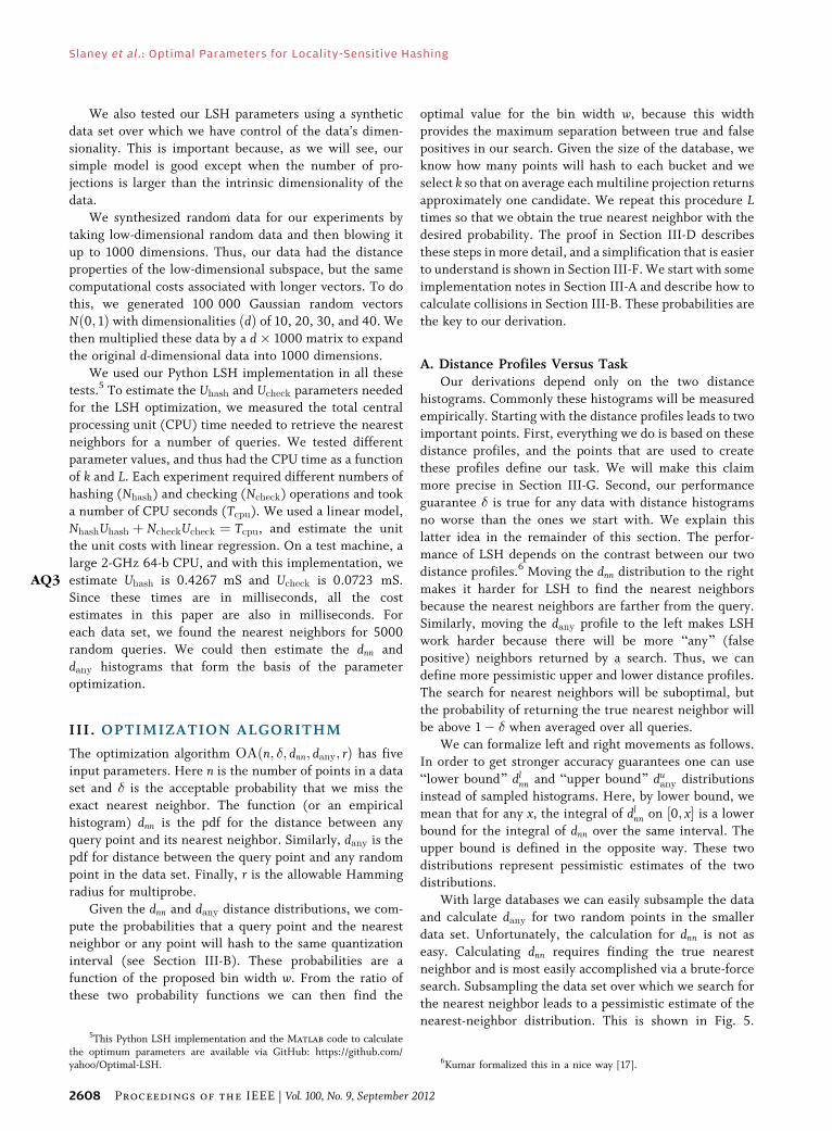
B. MultiprobeMultiprobe is a popular enhancement to LSH [18]. It is
based on the observation that a query’s nearest neighbors
might not be in the query’s bucket, and perhaps we should
look in nearby buckets as well. There are many ways to
find nearby buckets. For the analysis in this paper, we
consider a simple approach based on the Hamming dis-
tance. This idea is shown in Fig. 4, where a query is shown
after quantization in two of the k projection directions. Fora Hamming distance of radius r, we look at all buckets thatdiffer in at most r of the k projection coordinates. We only
consider the side of the 1-D query bucket closest to the
query.2 Thus, there are Crk buckets at a Hamming distance
of r from the query bucket.
We should note that choosing multiprobe bins by using
the Hamming distance is suboptimal compared to mea-
suring the exact distance between the query and the
nearest corner of any other neighboring bin [18]. Wesimplify our analysis by using the Hamming distance and
this provides guidance for the most common and useful
case when r ¼ 1.
Looking for data within a small Hamming radius, after
projecting and binary quantization, is common in the
computer-vision literature. Here we note that many
researchers are doing a form of multiprobe, as we define
it in this paper [13]. Salakhutdinov [23] uses a deep beliefnetwork to create a bit vector (with k ¼ 20, 30, and 128 b)
to represent an image. He then measures distance with a
Hamming metric (for example, r ¼ 4 or 5). Weiss [26]
describes how to create optimal projections and splits
using the graph Laplacian. Their graph encodes imagesimilarity and they split the graph to minimize the cuts.
He [11] and Jegou [15] look for projections that contain
maximal information. All of these approaches use a
Hamming metric to measure simularity and are analogous
to LSH with just one table ðL ¼ 1Þ. Similarly, a product
quantizer [14] uses the product of k vector quantizers to
define a bucket. Each quantizer only sees a subset of the
overall vector dimensions and thus each quantizer isanalogous to a trivial, axis-aligned projection.
C. Cost ModelWe optimize retrieval performance, given the desired
error requirement �, using a simple computational model.
For the search phase, we use unit costs Uhash and Ucheck.
Here, Uhash is an upper bound (for any practical value of k)of the cost for computing the location of the bin
corresponding to the query point, while Ucheck is a cost
of computing a distance between a candidate point and a
query point. We suppress the dependence on k here fortwo reasons: 1) in practice, arithmetic operations are
cheap compared to memory lookups; and 2) it allows us to
greatly simplify the choice of optimal parameters of LSH.
Essentially, we just ignore the benefit that smaller k givesto query hashing, and optimize the total sum of all other
costs.
Thus, the total costs of LSH are3
search time: LUhash þ jcandidatesjUcheck (1)
and the memory cost for the index is
index space: Ln: (2)
D. Experimental DataWe use two different data sets to demonstrate the
optimization calculations that follow and verify their per-formance. For all tests, the design specification ð�Þrequired that the true nearest neighbor be retrieved with
a probability of 1� � ¼ 0:5.Our real-world data are derived from a data set of more
than 850 000 images of European cities. We analyzed the
first 100 000 images with a convolutional deep-belief
network (DBN) [12] that produced a 1024-dimensional
feature vector for each image.4 This feature vector per-formed well in an image-classification experiment, so it
is a good data set for nearest-neighbor queries. We see
similar performance with features based on audio
modulation.
Fig. 4. Hamming distance in quantized projection space. Quantized
projections convert the original feature space into rectangular buckets
in a k-dimensional space. Multiprobe looks in nearby buckets to
find likely matches. Here we show the adjacent buckets in just
two of the k dimensions.
2This is a one-sided version of multiprobe. One could look on bothsides of the query bucket and all that changes in our derivation is the �0
function shown in Fig. 7. But with large bucket sizes, this is not necessary.
3Pauleve’ uses the same cost function [22, eq. (3)].4This R7 EC1M data set is available through Yahoo’s WebScope
program at http://webscope.sandbox.yahoo.com/catalog.php?datatype=r.
Slaney et al. : Optimal Parameters for Locality-Sensitive Hashing
Vol. 100, No. 9, September 2012 | Proceedings of the IEEE 2607
We also tested our LSH parameters using a syntheticdata set over which we have control of the data’s dimen-
sionality. This is important because, as we will see, our
simple model is good except when the number of pro-
jections is larger than the intrinsic dimensionality of the
data.
We synthesized random data for our experiments by
taking low-dimensional random data and then blowing it
up to 1000 dimensions. Thus, our data had the distanceproperties of the low-dimensional subspace, but the same
computational costs associated with longer vectors. To do
this, we generated 100 000 Gaussian random vectors
Nð0; 1Þ with dimensionalities ðdÞ of 10, 20, 30, and 40. We
then multiplied these data by a d� 1000 matrix to expand
the original d-dimensional data into 1000 dimensions.
We used our Python LSH implementation in all these
tests.5 To estimate the Uhash and Ucheck parameters neededfor the LSH optimization, we measured the total central
processing unit (CPU) time needed to retrieve the nearest
neighbors for a number of queries. We tested different
parameter values, and thus had the CPU time as a function
of k and L. Each experiment required different numbers of
hashing (Nhash) and checking (Ncheck) operations and took
a number of CPU seconds (Tcpu). We used a linear model,
NhashUhash þ NcheckUcheck ¼ Tcpu, and estimate the unitthe unit costs with linear regression. On a test machine, a
large 2-GHz 64-b CPU, and with this implementation, we
estimate Uhash is 0.4267 mS and Ucheck is 0.0723 mSAQ3 .
Since these times are in milliseconds, all the cost
estimates in this paper are also in milliseconds. For
each data set, we found the nearest neighbors for 5000
random queries. We could then estimate the dnn and
dany histograms that form the basis of the parameteroptimization.
III . OPTIMIZATION ALGORITHM
The optimization algorithm OAðn; �; dnn; dany; rÞ has five
input parameters. Here n is the number of points in a data
set and � is the acceptable probability that we miss theexact nearest neighbor. The function (or an empirical
histogram) dnn is the pdf for the distance between any
query point and its nearest neighbor. Similarly, dany is thepdf for distance between the query point and any random
point in the data set. Finally, r is the allowable Hamming
radius for multiprobe.
Given the dnn and dany distance distributions, we com-
pute the probabilities that a query point and the nearestneighbor or any point will hash to the same quantization
interval (see Section III-B). These probabilities are a
function of the proposed bin width w. From the ratio of
these two probability functions we can then find the
optimal value for the bin width w, because this widthprovides the maximum separation between true and false
positives in our search. Given the size of the database, we
know how many points will hash to each bucket and we
select k so that on average each multiline projection returns
approximately one candidate. We repeat this procedure Ltimes so that we obtain the true nearest neighbor with the
desired probability. The proof in Section III-D describes
these steps in more detail, and a simplification that is easierto understand is shown in Section III-F. We start with some
implementation notes in Section III-A and describe how to
calculate collisions in Section III-B. These probabilities are
the key to our derivation.
A. Distance Profiles Versus TaskOur derivations depend only on the two distance
histograms. Commonly these histograms will be measured
empirically. Starting with the distance profiles leads to two
important points. First, everything we do is based on these
distance profiles, and the points that are used to createthese profiles define our task. We will make this claim
more precise in Section III-G. Second, our performance
guarantee � is true for any data with distance histograms
no worse than the ones we start with. We explain this
latter idea in the remainder of this section. The perfor-
mance of LSH depends on the contrast between our two
distance profiles.6 Moving the dnn distribution to the right
makes it harder for LSH to find the nearest neighborsbecause the nearest neighbors are farther from the query.
Similarly, moving the dany profile to the left makes LSH
work harder because there will be more Bany[ (false
positive) neighbors returned by a search. Thus, we can
define more pessimistic upper and lower distance profiles.
The search for nearest neighbors will be suboptimal, but
the probability of returning the true nearest neighbor will
be above 1� � when averaged over all queries.We can formalize left and right movements as follows.
In order to get stronger accuracy guarantees one can use
Blower bound[ dlnn and Bupper bound[ duany distributions
instead of sampled histograms. Here, by lower bound, we
mean that for any x, the integral of dlnn on ½0; x� is a lowerbound for the integral of dnn over the same interval. The
upper bound is defined in the opposite way. These two
distributions represent pessimistic estimates of the twodistributions.
With large databases we can easily subsample the data
and calculate dany for two random points in the smaller
data set. Unfortunately, the calculation for dnn is not as
easy. Calculating dnn requires finding the true nearest
neighbor and is most easily accomplished via a brute-force
search. Subsampling the data set over which we search for
the nearest neighbor leads to a pessimistic estimate of thenearest-neighbor distribution. This is shown in Fig. 5.
5This Python LSH implementation and the Matlab code to calculatethe optimum parameters are available via GitHub: https://github.com/yahoo/Optimal-LSH. 6Kumar formalized this in a nice way [17].
Slaney et al.: Optimal Parameters for Locality-Sensitive Hashing
2608 Proceedings of the IEEE | Vol. 100, No. 9, September 2012
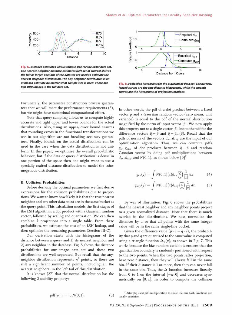
Fortunately, the parameter construction process guaran-
tees that we will meet the performance requirements ð�Þ,but we might have suboptimal computational effort.
Note that query sampling allows us to compute highlyaccurate and tight upper and lower bounds for the actual
distributions. Also, using an upper/lower bound ensures
that rounding errors in the functional transformations we
use in our algorithm are not breaking accuracy guaran-
tees. Finally, bounds on the actual distributions can be
used in the case when the data distribution is not uni-
form. In this paper, we optimize the overall probabilistic
behavior, but if the data or query distribution is dense inone portion of the space then one might want to use a
specially crafted distance distribution to model the inho-
mogenous distribution.
B. Collision ProbabilitiesBefore deriving the optimal parameters we first derive
expressions for the collision probabilities due to projec-
tions. We want to know how likely it is that the true nearest
neighbor and any other data point are in the same bucket as
the query point. This calculation models the first stages of
the LSH algorithm: a dot product with a Gaussian randomvector, followed by scaling and quantization. We can then
combine k projections into a single table. From these
probabilities, we estimate the cost of an LSH lookup, and
then optimize the remaining parameters (Section III-C).
Our derivation starts with the histograms of the
distance between a query and 1) its nearest neighbor and
2) any neighbor in the database. Fig. 5 shows the distance
probabilities for our image data set and these twodistributions are well separated. But recall that the any-
neighbor distribution represents n2 points, so there are
still a significant number of points, including all the
nearest neighbors, in the left tail of this distribution.
It is known [27] that the normal distribution has the
following 2-stability property:
pdf �p � �v ¼ jpjNð0; 1Þ: (3)
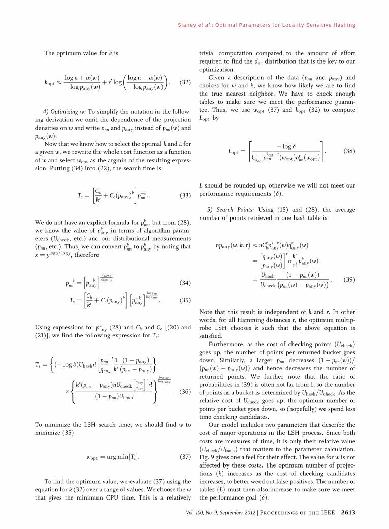
In other words, the pdf of a dot product between a fixed
vector �p and a Gaussian random vector (zero mean, unit
variance) is equal to the pdf of the normal distribution
magnified by the norm of input vector j�pj. We now apply
this property not to a single vector j�pj, but to the pdf for thedifference vectors �q� �p and �q� �pnnð�qÞ. Recall that thepdfs of norms of the vectors dnn; dany are the input of our
optimization algorithm. Thus, we can compute pdfs
gnn; gany of dot products between �q� �p and random
Gaussian vector by doing pdf multiplications between
dnn; dany and Nð0; 1Þ, as shown below [9]7
gnnðyÞ ¼Z
Nð0; 1ÞðxÞdnny
x
� � 1
jxj dx (4)
ganyðyÞ ¼Z
Nð0; 1ÞðxÞdanyy
x
� � 1
jxj dx: (5)
By way of illustration, Fig. 6 shows the probabilities
that the nearest neighbor and any neighbor points project
to a given normalized distance. Note that there is much
overlap in the distributions. We next normalize thedistances by w so that all points with the same integer
value will be in the same single-line bucket.
Given the difference value ð�p � �v� �q � �vÞ, the probabil-
ity that p and q are quantized to the same value is computed
using a triangle function �wðxÞ, as shown in Fig. 7. This
works because the bias random variable b ensures that thequantization boundary is randomly positioned with respect
to the two points. When the two points, after projection,have zero distance, then they will always fall in the same
bin. If their distance is 1 or more, then they can never fall
in the same bin. Thus, the � function increases linearly
from 0 to 1 on the interval ½�w; 0� and decreases sym-
metrically on ½0;w�. In order to compute the collision
7Datar [6] used pdf multiplication to show that his hash functions arelocally sensitive.
Fig. 6. Projectionhistograms for the EC1M image data set. The narrow,
jagged curves are the raw distance histograms, while the smooth
curves are the histograms of projection locations.
Fig. 5. Distance estimates versus sample size for the EC1M data set.
The nearest-neighbor distance estimates (left set of curves) shift to
the left as larger portions of the data set are used to estimate the
nearest-neighbor distribution. The any-neighbor distribution is an
unbiased estimate no matter what sample size is used. There are
870 000 images in the full data set.
Slaney et al. : Optimal Parameters for Locality-Sensitive Hashing
Vol. 100, No. 9, September 2012 | Proceedings of the IEEE 2609

probabilities for a nearest-neighbor �pnn and average �panypoint we should integrate the product of g and �
pnnðwÞ ¼Z
gnnðxÞ�wðxÞ dx (6)
panyðwÞ ¼Z
ganyðxÞ�wðxÞ dx: (7)
A similar collision calculation applies for multiprobe.
Fig. 7 also shows the �0 function that corresponds to the
simplest multiprobe case, a one-sided search. The query
point falls in the right half of its (1-D) bucket and we want
to know the probability that a candidate point with thegiven distance falls in the next bucket to the right.
This probability distribution starts at 0 for zero distance
because the query and the candidate are just separated by
the boundary. For distances between 0.5 and 1.0, the
probability is equal to 1.0 because at those distances the
candidate can only be in the adjacent bin. The probability
goes to zero as the distance approaches 1.5 because at these
distances the candidate point is likely to be two bucketsaway from the query’s bucket. Note that the calculation is
symmetric. We show �0 for the right-hand side adjacent
bin, which is used when the query is on the right-hand side
of its bucket, but the same equation holds on the left.
Thus, the probability that the query and its nearest
neighbor fall into adjacent bins is
qnnðwÞ ¼Z
gnnðxÞ�0wðxÞ dx: (8)
Note that we use q, instead of p, to represent the proba-
bilities of falling in the adjacent bin. Similarly, the proba-
bility that the query and any other point fall into adjacent
bin is
qanyðwÞ ¼Z
ganyðxÞ�0wðxÞ dx: (9)
Fig. 8 shows the critical distributions that are the basis
of our optimization algorithm. We show both theoretical
(solid lines) and experimental (marked points) results for
the EC1M image data set. We calculate the distance pro-
files empirically, as shown in Fig. 5, and from these pro-files we use (6) and (7) to compute the expected collision
probabilities pnn and pany. Both these probabilities are
functions of w. We use a similar process for the qprobabilities.
We implemented the LSH algorithm described here
using a combination of Python and NumPy. We then built
LSH indices with a wide range of quantization intervals
ðwÞ and measured the system’s performance. The discretepoints are empirical measurements of collision probabili-
ties (with k ¼ 1 and L ¼ 1). The measured distance pro-
files and probability calculations do a good job of
predicting the empirical probabilities shown in Fig. 8.
C. Combining ProjectionsOur model assumes that each projection is indepen-
dent of the others. Thus, we can combine the probabilities
of different projections and the probes of adjacent bins.
The probability that a query and its nearest neighbor fall
into the same k-dimensional bucket is equal to
pnnðw; kÞ ¼ pknnðwÞ: (10)
Then, the probability that two points have a Hamming
distance � r in one table is
pnnðw; k; rÞ ¼ pknnðwÞ þ kpk�1nn ðwÞqnnðwÞþ � � � þ Cr
kpk�rnn ðwÞqrnnðwÞ: (11)
Fig. 8. Bucket collision probabilities as a function of bin width for
the EC1M data set of photos. All probabilities start at 0, since the
collision probabilities are infinitesimally small with small buckets.
The two sigmoid curves show the probabilities for the query’s bucket.
The two unimodal curves show the collision probability for the
data in the adjacent bin. The left curve in each set is the probability
of finding the nearest neighbor, and the right curve is any other point.
Fig. 7. These windows give bucket probabilities as a function of
distance. The triangle is DwðxÞ and describes the probability that
a data point at a distance of x is in the same bucket as the query.
The trapezoid is D0wðxÞ and describes the same probability for the
closest adjacent bucket, given that we know the query is in the
right half of its bucket.
Slaney et al.: Optimal Parameters for Locality-Sensitive Hashing
2610 Proceedings of the IEEE | Vol. 100, No. 9, September 2012

In practice, we only consider small r, like r ¼ 0; 1; 2. Sincer � k, we note
pknnðwÞ � kpk�1nn ðwÞqnnðwÞ � Cr
kpk�rnn ðwÞqrnnðwÞ (12)
and hence we only need the last term of (11)
pnnðw; k; rÞ � Crkp
k�rnn ðwÞqrnnðwÞ: (13)
Similarly, the probability that any two points have a
Hamming distance � r in one table is
panyðw; k; rÞ ¼ pkanyðwÞ þ kpk�1anyðwÞqanyðwÞ
þ � � � þ Crkp
k�ranyðwÞqranyðwÞ (14)
and we approximate pany by
panyðw; k; rÞ � Crkp
k�ranyðwÞqranyðwÞ: (15)
From the original distance data, we have calculated the
collision probabilities. We can now derive the optimal LSHparameters.
D. Theoretical Analysis
Theorem 1: Let dnn, dany be the pdf for j�q� �pj distancesfor some data set distribution D and a query distribution
Q. Then, the following statements are true.
1) LSH with parameters OA.parameters ðn; �; dnn;dany; rÞ works in expected time OA.search_costðn;�; dnn; dany; rÞ time.
2) It returns the exact nearest neighbor with
probability at least 1� �.3) Parameter selection is optimal for any data set/
query distributions with the given distance profile
ðdnn; danyÞ.Proof: We work backwards to derive the optimal
parameters. We predict the optimal number of tables L by
hypothesizing values of w and k. Given an estimate of L, wefind the k that minimizes the search time cost. We then
plug our estimate of k and L to find the minimum searchcost and thus find the best w.
1) Optimizing L: Given the collision probabilities as
functions of w, we examine the steps of the optimization
algorithm in reverse order. Assume that parameters k andw are already selected. Then, we have to select a minimal Lthat puts the error probability below �. Given w and k, the
probability that we will do all these projections and stillmiss the nearest neighbor is equal to
1� pnnðw; k; rÞð ÞL� �
log 1� pnnðw; k; rÞð ÞL � logð�Þ: (16)
Let us use the approximation logð1� zÞ � �z here forð1� pnnðw; k; rÞÞ; this is fair since in real settings
pnnðw; k; rÞ is of order of 1=n [see (46)]. Thus, once wefind k and w, we should use (13) to find
Lopt ¼� log �
pnnðw; k; rÞ� � log �
Crkp
k�rnn ðwÞqrnnðwÞ
: (17)
This is optimum, given the values of w, k, and r. Usingfewer tables will reduce the computational effort but will
not meet the error guarantee. Using more tables will
further (unnecessarily) reduce the likelihood of missing
the true nearest neighbor, below �, and create more work.
2) Search Cost: The time to search an LSH database forone query’s nearest neighbors is8
Ts ¼ UhashLþ UcheckLnpanyðw; k; rÞ: (18)
With this computational model, the search time is
Ts ¼ Uhash� log �
Crkp
k�rnn ðwÞqrnnðwÞ
þUchecknð� log �ÞCrkp
k�ranyðwÞqranyðwÞ
Crkp
k�rnn ðwÞqrnnðwÞ
: (19)
We call this our exact cost model because the only
approximations are the independence assumption in (10),
which is hard not to do, and (12), which is true in all cases
we have seen. One could optimize LSH by performing a
brute-force search for the parameters w and k thatminimize this expression. These calculations are relatively
inexpensive because we have abstracted the data into the
two distance histograms.
We can simplify this cost function to derive explicit
expressions for the LSH parameters. We note r � k and
8A more accurate estimate of the search time is: Ts ¼ UhashLþUbinC
rkLþ UcheckLnpanyðw; k; rÞ where Ubin is the cost to locate one bin. In
practice, we only use small r, like r ¼ 0; 1; 2.Moreover,Ubin is usually muchsmaller than Uhash. In practice, Uhash consists of tens of inner products for ahigh-dimensional feature vector, while Ubin is just a memory locationoperation. So we can assume UbinC
rk � Uhash. And hence, search time can
still be approximated as UhashLþ UcheckLnpanyðw; k; rÞ.
Slaney et al. : Optimal Parameters for Locality-Sensitive Hashing
Vol. 100, No. 9, September 2012 | Proceedings of the IEEE 2611

Crk � kr=r!. Furthermore, we define the following twoexpressions (to allow us to isolate terms with k):
Ch ¼ Uhashð� log �Þr! pnnðwÞqnnðwÞ
� �r(20)
and
Cc ¼ Uchecknð� log �Þ pnnðwÞqnnðwÞ
qanyðwÞpanyðwÞ
� �r: (21)
Now the search time can be rewritten as
Ts ¼Ch
krpknnðwÞþ Cc
panyðwÞpnnðwÞ
� �k
: (22)
3) Optimizing k: The above expression is a sum of twostrictly monotonic functions of k: the first term increases
with k since pnnðwÞ is less than one, while the second is an
exponential with a base less than one since pany is alwayssmaller than pnn. It is difficult to find the exact optimum
for this expression. Instead, we find the value for k such
that the costs for k and kþ 1 are equalVthe minimum will
be in between. That is, we need to solve the equation
ChkrpknnðwÞ
þ CcpanyðwÞpnnðwÞ
� �k
¼ Chðkþ 1Þrpkþ1
nn ðwÞ þ CcpanyðwÞpnnðwÞ
� �kþ1
: (23)
Note that ððkþ 1Þr=krÞ ¼ ½ð1þ 1=kÞk�ðr=kÞ � er=k and
since r � k, then er=k is very close to 1. So
ChkrpknnðwÞ
þ CcpanyðwÞpnnðwÞ
� �k
¼ Chðkþ 1Þrpkþ1
nn ðwÞ þ CcpanyðwÞpnnðwÞ
� �kþ1
� Chkrpkþ1
nn ðwÞ þ CcpanyðwÞpnnðwÞ
� �kþ1
(24)
or by multiplying both sides by krpkþ1nn ðwÞ
ChpnnðwÞ þ CckrpkanyðwÞpnnðwÞ ¼ Ch þ Ccp
kþ1anyðwÞkr: (25)
With simplification, we have
CcpkanyðwÞkr pnnðwÞ � panyðwÞ
� �¼ Ch 1� pnnðwÞð Þ (26)
or in other words
pkanyðwÞ ¼Ch 1� pnnðwÞð Þ
Cckr pnnðwÞ � panyðwÞ : (27)
Putting the definition of Cc and Ch into the above, we
have
pkanyðwÞ ¼Ch 1� pnnðwÞð Þ
Cckr pnnðwÞ � panyðwÞ
¼
Uhash
Ucheck1� pnnðwÞð Þr!
kr pnnðwÞ � panyðwÞ
nqanyðwÞpanyðwÞ
� �r : (28)
Thus, the optimum k is defined by the fixed point
equation
k ¼ log nþ r log kþ �ðwÞ� log panyðwÞ
(29)
where
�ðwÞ ¼ logpnnðwÞ � panyðwÞ
1� pnnðwÞþ r log
qanyðwÞpanyðwÞ
þ logUcheck
Uhash� logðr!Þ: (30)
We wish to find a value for k that makes both sides of
this equation equal. First, define k0 ¼ ðlog nþ �ðwÞÞ=� log panyðwÞ so we can express k as a linear function of r
k � k0 þ r� log panyðwÞ logðk0Þ ¼ k0 þ r0 logðk0Þ: (31)
Putting this approximation into both sides of (29) gives
us k0þ r0 logðk0 þ r0 logðk0ÞÞ ¼ k0 þ r0 logðk0Þþr0 logð1þr0ðlogðk0Þ=k0ÞÞ. The difference between the left- and right-hand sides is �r0 logð1þ r0ðlogðk0Þ=k0ÞÞ, which is small
and close to 0. So k ¼ k0 þ r0 logðk0Þ is a good approximate
solution for (29).
Slaney et al.: Optimal Parameters for Locality-Sensitive Hashing
2612 Proceedings of the IEEE | Vol. 100, No. 9, September 2012
The optimum value for k is
kopt �log nþ �ðwÞ� log panyðwÞ
þ r0 loglog nþ �ðwÞ� log panyðwÞ
� �: (32)
4) Optimizing w: To simplify the notation in the follow-
ing derivation we omit the dependence of the projection
densities on w and write pnn and pany instead of pnnðwÞ andpanyðwÞ.
Now that we know how to select the optimal k and L fora given w, we rewrite the whole cost function as a function
of w and select wopt as the argmin of the resulting expres-sion. Putting (34) into (22), the search time is
Ts ¼Chkr
þ CcðpanyÞk� �
p�knn : (33)
We do not have an explicit formula for pknn, but from (28),
we know the value of pkany in terms of algorithm param-
eters (Ucheck, etc.) and our distributional measurements
(pnn, etc.). Thus, we can convert pknn to pkany by noting that
x ¼ ylog x= log y, therefore
p�knn ¼ p�k
any
h i log pnnlog pany
(34)
Ts ¼Chkr
þ CcðpanyÞk� �
p�kany
h i log pnnlog pany
: (35)
Using expressions for pkany (28) and Ch and Cc [(20) and(21)], we find the following expression for Ts:
Ts ¼ ð� log �ÞUhashr!pnnqnn
� �r1
krð1� panyÞðpnn � panyÞ
� �
�krðpnn � panyÞnUcheck
qanypany
h irr!
ð1� pnnÞUhash
8<:
9=;
log pnnlog pany
: (36)
To minimize the LSH search time, we should find w to
minimize (35)
wopt ¼ argmin½Ts�: (37)
To find the optimum value, we evaluate (37) using the
equation for k (32) over a range of values. We choose the wthat gives the minimum CPU time. This is a relatively
trivial computation compared to the amount of effortrequired to find the dnn distribution that is the key to our
optimization.
Given a description of the data (pnn and pany) and
choices for w and k, we know how likely we are to find
the true nearest neighbor. We have to check enough
tables to make sure we meet the performance guaran-
tee. Thus, we use wopt (37) and kopt (32) to compute
Lopt by
Lopt ¼� log �
Crkopt
pkopt�rnn ðwoptÞqrnnðwoptÞ
& ’: (38)
L should be rounded up, otherwise we will not meet our
performance requirements ð�Þ.
5) Search Points: Using (15) and (28), the average
number of points retrieved in one hash table is
npanyðw; k; rÞ � nCrkp
k�ranyðwÞqranyðwÞ
¼ qanyðwÞpanyðwÞ
� �rnkr
r!pkanyðwÞ
¼ Uhash
Ucheck
1� pnnðwÞð ÞpnnðwÞ � panyðwÞ : (39)
Note that this result is independent of k and r. In otherwords, for all Hamming distances r, the optimum multip-
robe LSH chooses k such that the above equation is
satisfied.
Furthermore, as the cost of checking points ðUcheckÞgoes up, the number of points per returned bucket goes
down. Similarly, a larger pnn decreases ð1� pnnðwÞÞ=ðpnnðwÞ � panyðwÞÞ and hence decreases the number of
returned points. We further note that the ratio ofprobabilities in (39) is often not far from 1, so the number
of points in a bucket is determined by Uhash=Ucheck. As the
relative cost of Ucheck goes up, the optimum number of
points per bucket goes down, so (hopefully) we spend less
time checking candidates.
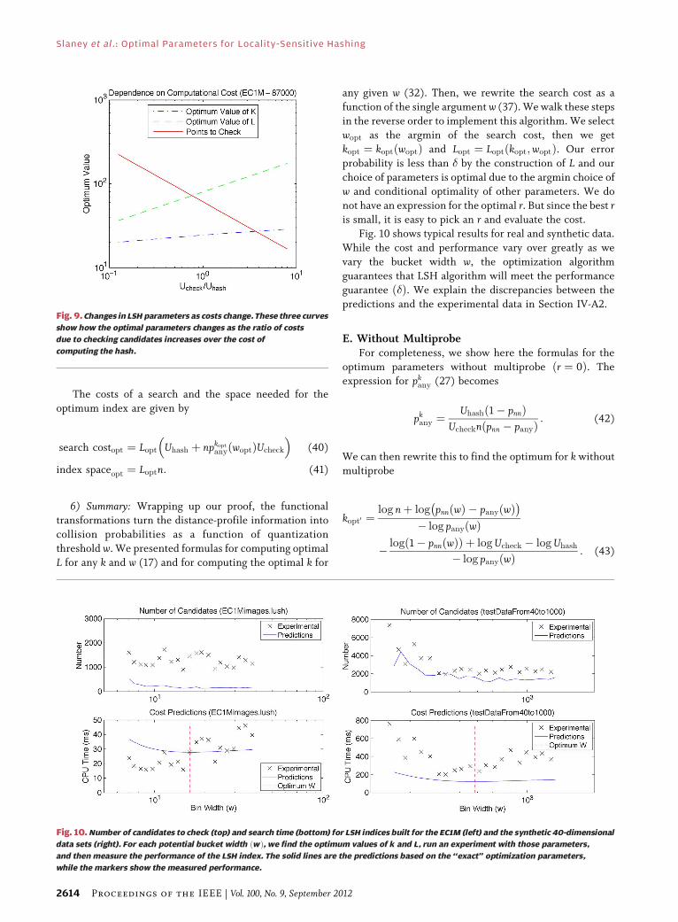
Our model includes two parameters that describe the
cost of major operations in the LSH process. Since both
costs are measures of time, it is only their relative valueðUcheck=UhashÞ that matters to the parameter calculation.
Fig. 9 gives one a feel for their effect. The value for w is not
affected by these costs. The optimum number of projec-
tions ðkÞ increases as the cost of checking candidates
increases, to better weed out false positives. The number of
tables ðLÞ must then also increase to make sure we meet
the performance goal ð�Þ.
Slaney et al. : Optimal Parameters for Locality-Sensitive Hashing
Vol. 100, No. 9, September 2012 | Proceedings of the IEEE 2613
The costs of a search and the space needed for the
optimum index are given by
search costopt ¼ Lopt Uhash þ npkoptanyðwoptÞUcheck
� �(40)
index spaceopt ¼ Loptn: (41)
6) Summary: Wrapping up our proof, the functionaltransformations turn the distance-profile information into
collision probabilities as a function of quantization
threshold w. We presented formulas for computing optimal
L for any k and w (17) and for computing the optimal k for
any given w (32). Then, we rewrite the search cost as afunction of the single argument w (37). We walk these steps
in the reverse order to implement this algorithm. We select
wopt as the argmin of the search cost, then we get
kopt ¼ koptðwoptÞ and Lopt ¼ Loptðkopt;woptÞ. Our error
probability is less than � by the construction of L and our
choice of parameters is optimal due to the argmin choice of
w and conditional optimality of other parameters. We do
not have an expression for the optimal r. But since the best ris small, it is easy to pick an r and evaluate the cost.
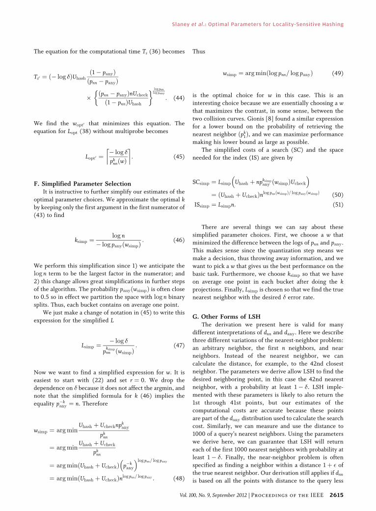
Fig. 10 shows typical results for real and synthetic data.
While the cost and performance vary over greatly as we
vary the bucket width w, the optimization algorithm
guarantees that LSH algorithm will meet the performance
guarantee ð�Þ. We explain the discrepancies between the
predictions and the experimental data in Section IV-A2.
E. Without MultiprobeFor completeness, we show here the formulas for the
optimum parameters without multiprobe ðr ¼ 0Þ. Theexpression for pkany (27) becomes
pkany ¼Uhashð1� pnnÞ
Uchecknðpnn � panyÞ: (42)
We can then rewrite this to find the optimum for k withoutmultiprobe
kopt0 ¼log nþ log pnnðwÞ � panyðwÞ
� log panyðwÞ
� log 1� pnnðwÞð Þ þ logUcheck � logUhash
� log panyðwÞ: (43)
Fig. 10. Number of candidates to check (top) and search time (bottom) for LSH indices built for the EC1M (left) and the synthetic 40-dimensional
data sets (right). For each potential bucket width ðwÞ, we find the optimum values of k and L, run an experiment with those parameters,
and then measure the performance of the LSH index. The solid lines are the predictions based on the ‘‘exact’’ optimization parameters,
while the markers show the measured performance.
Fig. 9. Changes in LSH parameters as costs change. These three curves
show how the optimal parameters changes as the ratio of costs
due to checking candidates increases over the cost of
computing the hash.
Slaney et al.: Optimal Parameters for Locality-Sensitive Hashing
2614 Proceedings of the IEEE | Vol. 100, No. 9, September 2012
The equation for the computational time Ts (36) becomes
Ts0 ¼ ð� log �ÞUhashð1� panyÞðpnn � panyÞ
� ðpnn � panyÞnUcheck
ð1� pnnÞUhash
� � log pnnlog pany
: (44)
We find the wopt0 that minimizes this equation. The
equation for Lopt (38) without multiprobe becomes
Lopt0 ¼� log �
pknnðwÞ
�: (45)
F. Simplified Parameter SelectionIt is instructive to further simplify our estimates of the
optimal parameter choices. We approximate the optimal kby keeping only the first argument in the first numerator of
(43) to find
ksimp ¼log n
� log panyðwsimpÞ: (46)
We perform this simplification since 1) we anticipate thelog n term to be the largest factor in the numerator; and
2) this change allows great simplifications in further steps
of the algorithm. The probability panyðwsimpÞ is often close
to 0.5 so in effect we partition the space with log n binary
splits. Thus, each bucket contains on average one point.
We just make a change of notation in (45) to write this
expression for the simplified L
Lsimp ¼ � log �
pksimpnn ðwsimpÞ
: (47)
Now we want to find a simplified expression for w. It iseasiest to start with (22) and set r ¼ 0. We drop the
dependence on � because it does not affect the argmin, and
note that the simplified formula for k (46) implies the
equality p�kany ¼ n. Therefore
wsimp ¼ argminUhash þ Uchecknp
kany
pknn
¼ argminUhash þ Ucheck
pknn
¼ argminðUhash þ UcheckÞ p�kany
� �log pnn= log pany
¼ argminðUhash þ UcheckÞnlog pnn= log pany : (48)
Thus
wsimp ¼ argminðlog pnn= log panyÞ (49)
is the optimal choice for w in this case. This is an
interesting choice because we are essentially choosing a wthat maximizes the contrast, in some sense, between the
two collision curves. Gionis [8] found a similar expressionfor a lower bound on the probability of retrieving the
nearest neighbor ðpk1Þ, and we can maximize performance
making his lower bound as large as possible.
The simplified costs of a search (SC) and the space
needed for the index (IS) are given by
SCsimp ¼ Lsimp Uhash þ npksimpany ðwsimpÞUcheck
� �¼ ðUhash þ UcheckÞnlog pnnðwsimpÞ= log panyðwsimpÞ (50)
ISsimp ¼ Lsimpn: (51)
There are several things we can say about these
simplified parameter choices. First, we choose a w that
minimized the difference between the logs of pnn and pany.This makes sense since the quantization step means we
make a decision, thus throwing away information, and we
want to pick a w that gives us the best performance on thebasic task. Furthermore, we choose ksimp so that we have
on average one point in each bucket after doing the kprojections. Finally, Lsimp is chosen so that we find the true
nearest neighbor with the desired � error rate.
G. Other Forms of LSHThe derivation we present here is valid for many
different interpretations of dnn and dany. Here we describethree different variations of the nearest-neighbor problem:
an arbitrary neighbor, the first n neighbors, and near
neighbors. Instead of the nearest neighbor, we can
calculate the distance, for example, to the 42nd closestneighbor. The parameters we derive allow LSH to find the
desired neighboring point, in this case the 42nd nearest
neighbor, with a probability at least 1� �. LSH imple-
mented with these parameters is likely to also return the
1st through 41st points, but our estimates of the
computational costs are accurate because these points
are part of the dany distribution used to calculate the searchcost. Similarly, we can measure and use the distance to1000 of a query’s nearest neighbors. Using the parameters
we derive here, we can guarantee that LSH will return
each of the first 1000 nearest neighbors with probability at
least 1� �. Finally, the near-neighbor problem is often
specified as finding a neighbor within a distance 1þ � ofthe true nearest neighbor. Our derivation still applies if dnnis based on all the points with distance to the query less
Slaney et al. : Optimal Parameters for Locality-Sensitive Hashing
Vol. 100, No. 9, September 2012 | Proceedings of the IEEE 2615

than dtrueð1þ �Þ where dtrue is the distance to the (empir-
ically measured) nearest neighbor.
More precisely, the distance distribution dnnðxÞ is aconditional probability
dnnðxÞ ¼ Pðdistanceðq; pÞ ¼ xjp belongs to
q0s nearest-neighbor subsetÞ: (52)
By this means, we can define a query’s nearest-neighborsubset in many different ways, and our theory will always
hold. In all cases, the performance guarantee becomes: we
guarantee to return any point �p in �q’s Bnearest-neighbor[subset with a probability of at least 1� �. Finally, to be
clear, we note that dnn, gnn, and pnn are all conditional
probabilities, depending on the definition of the nearest-
neighbor subset.
IV. EXPERIMENTS
We describe two types of experiments in this section:
validation and extensions. We first show that our theory
matches reality by testing an LSH implementation and
measuring its performance. This validates our optimization
approach in several different ways. Most importantly, weshow that we can predict collisions and the number of
points returned. We also show how multiprobe affects
performance. We use synthetic data for many of these
experiments because it is easier to talk about the char-
acteristics of the data. We see the same behavior with real
audio or image data (as shown in the illustrations of the
previous section). Second we use the theory describing
LSH’s behavior to discuss how LSH works on very largedatabases and to connect LSH and other approaches. We
performed all experiments using LSH parameters cal-
culated using the Bexact[ parameters from our optimi-
zation algorithm (not brute force or the simplified
approximations).
A. Experimental Validation
1) Combining Projections: Fig. 11 shows the number of
retrieved results as a function of the number of projections
ðkÞ for one table ðL ¼ 1Þ. We base the theory in Section III-Con the hypothesis that each projection is independent and
thus the theoretical probability that any one point (nearest
or any neighbor) remains after k projections is pk. However,we see that the theory underestimates the number of re-
trieved points, especially for large values of k. (The discre-pancy is smaller for the nearest-neighbor counts.)
The four panels of Fig. 11 suggest that the deviation is
related to the dimensionality of the data. In retrospect thismakes sense. The first k ¼ d projections are all linearly
independent of each other. The ðdþ 1Þth projection in a
d-dimensional space has to be a linear combination of the
first d projections. Independence (in a linear algebra
sense) is not the same as independence (in a statistical
sense). Our projections are correlated.
In the remaining simulations of this section, we also show
a Bcompensated[ prediction based on the experimentalperformance after the k projections. To gauge the discrep-
ancy when k > d, we do a simulation with the desired k andmeasure the true pany performance. This then forms a new
estimate of panyðw; k; rÞ that we plug into the rest of the
Fig. 11. Probability of finding any neighbor. These four panels show
the probability of finding the true nearest neighbor as a function of k
in four different synthetic data sets. Note the relative magnitude
of the discrepancy between theory and experiments for large k.
Fig. 12. Quality of the LSH results. These four panels show the
probability of finding the true nearest neighbor in four different
synthetic data sets. In each case, the design specification 1� �
requires that the correct answer be found more than
50% of the time.
Slaney et al.: Optimal Parameters for Locality-Sensitive Hashing
2616 Proceedings of the IEEE | Vol. 100, No. 9, September 2012

theory. This shows that most of the discrepancies that followare due to the (under) performance of the k projections.
2) Overall Results: Fig. 12 summarizes the quality of the
points retrieved by LSH for the four test dimensionalities.
These four panels show the probability of getting the true
nearest neighbor for a large number of random queries.
For each value of w around the theoretical optimum we
predict the best parameters (lowest CPU time) that meetthe � performance guarantee. We are thus showing opti-
mum performance for all values of w (although only one of
these bucket sizes will have the absolute minimal CPU
time). In all but one trial the measured retrieval accuracy
rate is greater than the 0:50 ¼ 1� � target.
Fig. 13 shows the number of points returned in all Lbuckets for all four dimensionalities. This result is im-
portant because it determines the number of points whichmust be checked. If we return too many points, then the
retrieval time is slow because they all require checking.
While there are discrepancies, the Bcompensated[ curve isa pretty good fit for the experimental results, especially for
the larger dimensionalities.
Fig. 14 shows the overall computational effort. These
tests were all performed on the same machine using our
implementation of LSH in Python. While the long vectorsmean that most of the work is done by the NumPy nume-
rical library, there is still overhead in Python for which we
are not accounting. In particular, the estimates are better
for the longer times, perhaps because this minimizes the
impact of the fixed overhead in a query.
Fig. 15 demonstrates the sensitivity of an LSH index to
its parameters. For each w and k, we select the L that meets
the performance guarantee and then plot the time it wouldtake such an index to answer one query. This figure shows
a long, narrow valley where the parameters are optimum.
This might explain the difficulty practitioners have in
finding the optimal parameters to make practical use ofLSH. Note that the curve in Fig. 10 shows the minimum
computation time as a function of just wVwe choose
optimum values for k and L. Thus, the 1-D curves of Fig. 14
follow the valley shown in Fig. 15.
Finally, we return to the real-world experimental re-
sults shown in Fig. 10. We believe that underestimating
the independence of the k projections, as shown in
Fig. 10, explains the discrepancy in the number of EC1M
Fig. 13. Number of LSH candidates. These four panels show the
number of candidates returned in an optimal implementation
of LSH, as a function of the bin width.
Fig. 14. CPU time per query. These four panels show the amount
of CPU time per query in an optimal implementation of LSH,
as a function of the bin width.
Fig. 15. CPU time as a function of k and w. At each point, we use the L
that guarantees we meet the performance guarantee, and thus costs
dramatically increase when the wrong parameters are used. The
minima found using the brute-force (*) and ‘‘exact’’ (x) calculations
are on top of each other. The simple estimate is close and is still in
the valley. All times are in milliseconds, and for display purposes,
we limited the maximum value to 1000 times the minimum value.
Slaney et al. : Optimal Parameters for Locality-Sensitive Hashing
Vol. 100, No. 9, September 2012 | Proceedings of the IEEE 2617
candidates. This suggests that the intrinsic dimensional-ity of this image feature data is low. Nevertheless, the
total CPU time is predicted with good accuracy, probably
because the query time is dominated by the Python
index. Our higher dimensional synthetic data are a better
fit to the model.
3) Multiprobe: Multiprobe offers its own advantages and
disadvantages. In the analysis in this paper, we limit theHamming distance between the query bucket and the
buckets we check. Better approaches might look at the true
distance to each bucket and thus might choose a bucket
with a Hamming distance of 2 before all the buckets with a
distance of 1 are exhausted [18]. Still most of the benefit
comes from the nearest bucket in each direction and this
simplification allows us to understand the advantages of
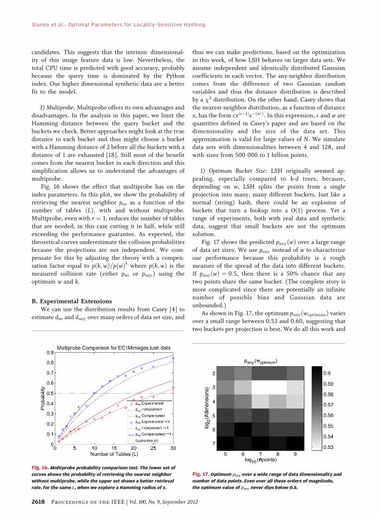
multiprobe.Fig. 16 shows the effect that multiprobe has on the
index parameters. In this plot, we show the probability of
retrieving the nearest neighbor pnn as a function of the
number of tables ðLÞ, with and without multiprobe.
Multiprobe, even with r ¼ 1, reduces the number of tables
that are needed, in this case cutting it in half, while still
exceeding the performance guarantee. As expected, the
theoretical curves underestimate the collision probabilitiesbecause the projections are not independent. We com-
pensate for this by adjusting the theory with a compen-
sation factor equal to pðk;wÞ=pðwÞk where pðk;wÞ is the
measured collision rate (either pnn or pany) using the
optimum w and k.
B. Experimental ExtensionsWe can use the distribution results from Casey [4] to
estimate dnn and dany over many orders of data set size, and
thus we can make predictions, based on the optimizationin this work, of how LSH behaves on larger data sets. We
assume independent and identically distributed Gaussian
coefficients in each vector. The any-neighbor distribution
comes from the difference of two Gaussian random
variables and thus the distance distribution is described
by a �2 distribution. On the other hand, Casey shows that
the nearest-neighbor distribution, as a function of distance
x, has the form cxðc�1Þe�ðwcÞ. In this expression, c and w arequantities defined in Casey’s paper and are based on the
dimensionality and the size of the data set. This
approximation is valid for large values of N. We simulate
data sets with dimensionalities between 4 and 128, and
with sizes from 500 000 to 1 billion points.
1) Optimum Bucket Size: LSH originally seemed ap-
pealing, especially compared to k-d trees, because,depending on w, LSH splits the points from a single
projection into many, many different buckets. Just like a
normal (string) hash, there could be an explosion of
buckets that turn a lookup into a Oð1Þ process. Yet a
range of experiments, both with real data and synthetic
data, suggest that small buckets are not the optimum
solution.
Fig. 17 shows the predicted panyðwÞ over a large rangeof data set sizes. We use pany instead of w to characterize
our performance because this probability is a rough
measure of the spread of the data into different buckets.
If panyðwÞ ¼ 0:5, then there is a 50% chance that any
two points share the same bucket. (The complete story is
more complicated since there are potentially an infinite
number of possible bins and Gaussian data are
unbounded.)As shown in Fig. 17, the optimum panyðwoptimumÞ varies
over a small range between 0.53 and 0.60, suggesting that
two buckets per projection is best. We do all this work and
Fig. 16. Multiprobe probability comparison test. The lower set of
curves shows the probability of retrieving the nearest neighbor
without multiprobe, while the upper set shows a better retrieval
rate, for the same L, when we explore a Hamming radius of 1.
Fig. 17. Optimum pany over a wide range of data dimensionality and
number of data points. Even over all these orders of magnitude,
the optimum value of pany never dips below 0.5.
Slaney et al.: Optimal Parameters for Locality-Sensitive Hashing
2618 Proceedings of the IEEE | Vol. 100, No. 9, September 2012
we end up with binary splits from each projection.9 This
result is also consistent with that shown, for example, in
Fig. 10, where the search cost only goes up slightly as wgets larger. This is the first demonstration that we know of
that shows the power of binary LSH. Over this wide range
of parameter values we see no case where a small w, andthus more bins per projection, is optimal.
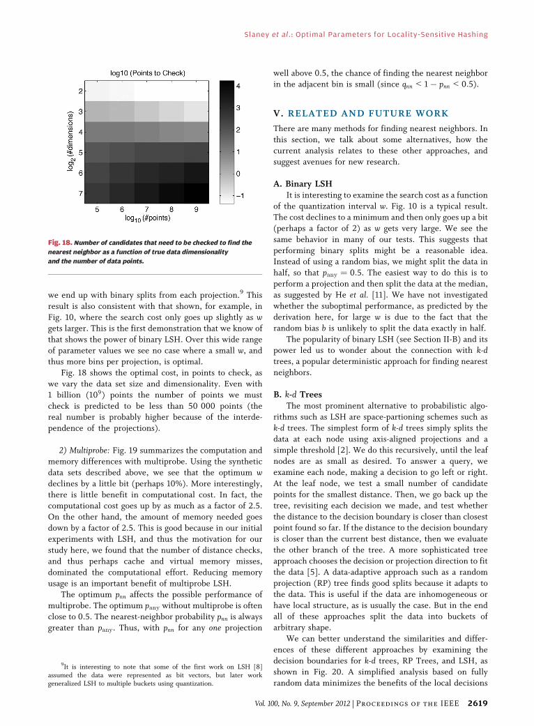
Fig. 18 shows the optimal cost, in points to check, as
we vary the data set size and dimensionality. Even with
1 billion (109) points the number of points we must
check is predicted to be less than 50 000 points (thereal number is probably higher because of the interde-
pendence of the projections).
2) Multiprobe: Fig. 19 summarizes the computation and
memory differences with multiprobe. Using the synthetic
data sets described above, we see that the optimum wdeclines by a little bit (perhaps 10%). More interestingly,
there is little benefit in computational cost. In fact, thecomputational cost goes up by as much as a factor of 2.5.
On the other hand, the amount of memory needed goes
down by a factor of 2.5. This is good because in our initial
experiments with LSH, and thus the motivation for our
study here, we found that the number of distance checks,
and thus perhaps cache and virtual memory misses,
dominated the computational effort. Reducing memory
usage is an important benefit of multiprobe LSH.The optimum pnn affects the possible performance of
multiprobe. The optimum pany without multiprobe is often
close to 0.5. The nearest-neighbor probability pnn is alwaysgreater than pany. Thus, with pnn for any one projection
well above 0.5, the chance of finding the nearest neighborin the adjacent bin is small (since qnn G 1� pnn G 0:5).
V. RELATED AND FUTURE WORK
There are many methods for finding nearest neighbors. In
this section, we talk about some alternatives, how the
current analysis relates to these other approaches, and
suggest avenues for new research.
A. Binary LSHIt is interesting to examine the search cost as a function
of the quantization interval w. Fig. 10 is a typical result.
The cost declines to a minimum and then only goes up a bit
(perhaps a factor of 2) as w gets very large. We see the
same behavior in many of our tests. This suggests that
performing binary splits might be a reasonable idea.Instead of using a random bias, we might split the data in
half, so that pany ¼ 0:5. The easiest way to do this is to
perform a projection and then split the data at the median,
as suggested by He et al. [11]. We have not investigated
whether the suboptimal performance, as predicted by the
derivation here, for large w is due to the fact that the
random bias b is unlikely to split the data exactly in half.
The popularity of binary LSH (see Section II-B) and itspower led us to wonder about the connection with k-dtrees, a popular deterministic approach for finding nearest
neighbors.
B. k-d TreesThe most prominent alternative to probabilistic algo-
rithms such as LSH are space-partioning schemes such as
k-d trees. The simplest form of k-d trees simply splits thedata at each node using axis-aligned projections and a
simple threshold [2]. We do this recursively, until the leaf
nodes are as small as desired. To answer a query, we
examine each node, making a decision to go left or right.
At the leaf node, we test a small number of candidate
points for the smallest distance. Then, we go back up the
tree, revisiting each decision we made, and test whether
the distance to the decision boundary is closer than closestpoint found so far. If the distance to the decision boundary
is closer than the current best distance, then we evaluate
the other branch of the tree. A more sophisticated tree
approach chooses the decision or projection direction to fit
the data [5]. A data-adaptive approach such as a random
projection (RP) tree finds good splits because it adapts to
the data. This is useful if the data are inhomogeneous or
have local structure, as is usually the case. But in the endall of these approaches split the data into buckets of
arbitrary shape.
We can better understand the similarities and differ-
ences of these different approaches by examining the
decision boundaries for k-d trees, RP Trees, and LSH, as
shown in Fig. 20. A simplified analysis based on fully
random data minimizes the benefits of the local decisions
9It is interesting to note that some of the first work on LSH [8]assumed the data were represented as bit vectors, but later workgeneralized LSH to multiple buckets using quantization.
Fig. 18. Number of candidates that need to be checked to find the
nearest neighbor as a function of true data dimensionality
and the number of data points.
Slaney et al. : Optimal Parameters for Locality-Sensitive Hashing
Vol. 100, No. 9, September 2012 | Proceedings of the IEEE 2619

in k-d trees. k-d trees especially shine when there is local
structure in the data, and the decisions made at one node
are quite different from that of another node. But still, it isuseful to consider this random (worst) case, especially
since the analysis is easier.
With uniform data, a k-d tree with a depth of k levels isanalogous to LSH with k (global) projections, a binary
decision where panyðwoptimumÞ ¼ 0:5, and L ¼ 1. Without
backtracking, a k-d tree is unlikely to retrieve the nearest
neighbor.
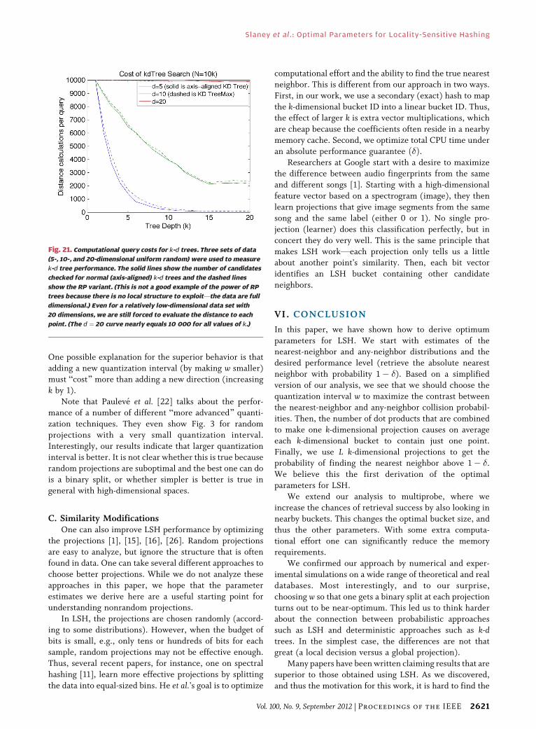
But with backtracking, a k-d tree can retrieve the exactnearest neighbor (with � ¼ 0). At each level of the tree,
the best branch is checked, and then the best or smallest
distance found so far is compared to the distance between
the query point and the decision boundary. If the best
distance so far is large enough, then we check the alternate
node. This can be painful, however, because if one checks
both sides of each node, then one checks the entire tree.
The computational cost of this kind of algorithm is shownin Fig. 21. Even with a relatively low dimensionality such
as 20 we are looking at all the data points. This is due to the
curse of dimensionality and the structure of the tree.
It is hard to make use of the neighborhood information
in a tree because its structure is inhomogenous. Due to the
local decisions at each node, a bucket nearby the tree
might not be adjacent in feature space to the query bucket.
Thus, backtracking is an exhaustive approach (compared tothe regular approach in multiprobe). One could be smarter
about checking alternative nodes, in a manner analogous
to multiprobe, and thus could check fewer buckets. But the
overall algorithm looks a lot like binary LSH with L ¼ 1. As
shown above, for homogeneous data, our LSH analysis
suggests that this is suboptimal.
A more powerful alternative is a forest of k-d trees [21],[20]. As implied by the name, multiple (random) trees arebuilt to answer the query. Backtracking is not performed;
instead the inherent randomness in the way the data are
grouped by different trees provides a degree of robustness
not found in a single tree. Thus, when the lookup is
performed with L k-d trees it has much of the same flavor
as LSH with L k-dimensional indices. It would be
interesting to analyze a forest of k-d trees using the
approach described here.Finally, binary LSH is interesting, especially since we
have found that under the optimum LSH parameters each
dot product is being used to split the data into two buckets.
By going with binary LSH, we give up on having an infinite
number of (potential) buckets but the analysis is simpler.
Fig. 20. Data buckets for two kinds of k-d trees and LSH. These three images show typical bucket shapes for random 2-D data using
axis-aligned four-level-deep k-d trees, RP trees, and LSH with four projections.
Fig. 19. Effect of LSHmultiprobe on number of candidates to check (left) andmemory (right). In both cases, the ratio of the original cost over the
multiprobe cost is calculated. For high values of the data dimensionality ðdÞ and number of points ðnÞ, multiprobe LSH with a Hamming radius
of 1 ðr ¼ 1Þ requires more candidate checking but reduces the memory usage, all the while maintaining the same performance guarantee ð�Þ.
Slaney et al.: Optimal Parameters for Locality-Sensitive Hashing
2620 Proceedings of the IEEE | Vol. 100, No. 9, September 2012
One possible explanation for the superior behavior is that
adding a new quantization interval (by making w smaller)must Bcost[ more than adding a new direction (increasing
k by 1).Note that Pauleve et al. [22] talks about the perfor-
mance of a number of different Bmore advanced[ quanti-
zation techniques. They even show Fig. 3 for random
projections with a very small quantization interval.
Interestingly, our results indicate that larger quantization
interval is better. It is not clear whether this is true becauserandom projections are suboptimal and the best one can do
is a binary split, or whether simpler is better is true in
general with high-dimensional spaces.
C. Similarity ModificationsOne can also improve LSH performance by optimizing
the projections [1], [15], [16], [26]. Random projections
are easy to analyze, but ignore the structure that is often
found in data. One can take several different approaches to
choose better projections. While we do not analyze these
approaches in this paper, we hope that the parameter
estimates we derive here are a useful starting point forunderstanding nonrandom projections.
In LSH, the projections are chosen randomly (accord-
ing to some distributions). However, when the budget of
bits is small, e.g., only tens or hundreds of bits for each
sample, random projections may not be effective enough.
Thus, several recent papers, for instance, one on spectral
hashing [11], learn more effective projections by splitting
the data into equal-sized bins. He et al.’s goal is to optimize
computational effort and the ability to find the true nearestneighbor. This is different from our approach in two ways.
First, in our work, we use a secondary (exact) hash to map
the k-dimensional bucket ID into a linear bucket ID. Thus,
the effect of larger k is extra vector multiplications, which
are cheap because the coefficients often reside in a nearby
memory cache. Second, we optimize total CPU time under
an absolute performance guarantee ð�Þ.Researchers at Google start with a desire to maximize
the difference between audio fingerprints from the same
and different songs [1]. Starting with a high-dimensional
feature vector based on a spectrogram (image), they then
learn projections that give image segments from the same
song and the same label (either 0 or 1). No single pro-
jection (learner) does this classification perfectly, but in
concert they do very well. This is the same principle that
makes LSH workVeach projection only tells us a littleabout another point’s similarity. Then, each bit vector
identifies an LSH bucket containing other candidate
neighbors.
VI. CONCLUSION
In this paper, we have shown how to derive optimum
parameters for LSH. We start with estimates of thenearest-neighbor and any-neighbor distributions and the
desired performance level (retrieve the absolute nearest
neighbor with probability 1� �). Based on a simplified
version of our analysis, we see that we should choose the
quantization interval w to maximize the contrast between
the nearest-neighbor and any-neighbor collision probabil-
ities. Then, the number of dot products that are combined
to make one k-dimensional projection causes on averageeach k-dimensional bucket to contain just one point.
Finally, we use L k-dimensional projections to get the
probability of finding the nearest neighbor above 1� �.We believe this the first derivation of the optimal
parameters for LSH.
We extend our analysis to multiprobe, where we
increase the chances of retrieval success by also looking in
nearby buckets. This changes the optimal bucket size, andthus the other parameters. With some extra computa-
tional effort one can significantly reduce the memory
requirements.
We confirmed our approach by numerical and exper-
imental simulations on a wide range of theoretical and real
databases. Most interestingly, and to our surprise,
choosing w so that one gets a binary split at each projection
turns out to be near-optimum. This led us to think harderabout the connection between probabilistic approaches
such as LSH and deterministic approaches such as k-dtrees. In the simplest case, the differences are not that
great (a local decision versus a global projection).
Many papers have been written claiming results that are
superior to those obtained using LSH. As we discovered,
and thus the motivation for this work, it is hard to find the
Fig. 21. Computational query costs for k-d trees. Three sets of data
(5-, 10-, and 20-dimensional uniform random) were used to measure
k-d tree performance. The solid lines show the number of candidates
checked for normal (axis-aligned) k-d trees and the dashed lines
show the RP variant. (This is not a good example of the power of RP
trees because there is no local structure to exploitVthe data are full
dimensional.) Even for a relatively low-dimensional data set with
20 dimensions, we are still forced to evaluate the distance to each
point. (The d ¼ 20 curve nearly equals 10 000 for all values of k.)
Slaney et al. : Optimal Parameters for Locality-Sensitive Hashing
Vol. 100, No. 9, September 2012 | Proceedings of the IEEE 2621

best parameter values using exhaustive search, especially inthe large databases that we find interesting. In this paper,
we do not claim that LSH is the best solution. Instead, we
hope that this paper, the analysis, and the optimization
algorithm we describe will be a good starting point for
anybody who wants to find nearest neighbors, using
random or deterministic algorithms. h
Acknowledgment
We are grateful for the assistance and comments we
received from K. Li (Princeton) and K. Grauman (Univ. ofTexas, Austin) and their students. A number of anony-
mous reviewers have also contributed good questions and
ideas.
REFERENCES
[1] S. Baluja and M. Covell, BLearning to hash:Forgiving hash functions and applications,[Data Mining Knowl. Disc., vol. 17, no. 3,pp. 402–430, Dec. 2008.
[2] J. L. Bentley, BMultidimensional binarysearch trees used for associative searching,[Commun. ACM, vol. 18, no. 9, pp. 509–517,1975.
[3] K. Beyer, J. Goldstein, R. Ramakrishnan, andU. Shaft, BWhen is Fnearest neighbor_meaningful?[ in Proc. Int. Conf. DatabaseTheory, 1998, pp. 217–235.
[4] M. A. Casey, C. Rhodes, and M. Slaney,BAnalysis of minimum distances inhigh-dimensional musical spaces,[ IEEETrans. Audio Speech Lang. Process., vol. 16,no. 5, pp. 1015–1028, Jul. 2008.
[5] S. Dasgupta and Y. Freund, BRandomprojection trees for vector quantization,[IEEE Trans. Inf. Theory, vol. 55, no. 7,pp. 3229–3242, Jul. 2009.
[6] M. Datar, N. Immorlica, P. Indyk, andV. S. Mirrokni, BLocality-sensitive hashingscheme based on p-stable distributions,[ inProc. 20th Annu. Symp. Comput. Geometry,2004, pp. 253–262.
[7] W. Dong, Z. Wang, W. Josephson,M. Charikar, and K. Li, BModeling LSHfor performance tuning,[ in Proc. 17thACM Conf. Inf. Knowl. Manage., 2008,pp. 669–678.
[8] A. Gionis, P. Indyk, and R. Motwani,BSimilarity search in high dimensionsvia hashing,[ in Proc. 25th Int. Conf. Very LargeData Bases, 1999, pp. 518–529.
[9] A. G. Glen, L. M. Leemis, and J. H. Drew,BComputing the distribution of the product oftwo continuous random variables,[ Comput.
Stat. Data Anal., vol. 44, no. 3, pp. 451–464,Jan. 2004.
[10] K. Grauman, BEfficiently searching for similarimages,[ Commun. ACM, vol. 53, no. 6,pp. 84–94, 2010.
[11] J. He, R. Radhakrishnan, S.-F. Chang, andC. Bauer, BCompact hashing with jointoptimization of search accuracy and time,[ inProc. IEEE Conf. Comput. Vis. Pattern Recognit.,Jun. 2011, pp. 753–760.
[12] E. Horster, M. Slaney, M. A. Ranzato, andK. Weinberger, BUnsupervised imageranking,[ in Proc. 1st ACM WorkshopLarge-Scale Multimedia Retrieval Mining,2009, pp. 81–88.
[13] H. Jegou, M. Douze, and C. Schmid,BHamming embedding and weak geometricconsistency for large scale image search,[ inProc. 10th Eur. Conf. Comput. Vis. I, Marseille,France, 2008, pp. 304–317.
[14] H. Jegou, M. Douze, and C. Schmid,BProduct quantization for nearest neighborsearch,[ IEEE Trans. Pattern Anal. Mach. Intell,vol. 33, no. 1, pp. 117–128, Jan. 2011.
[15] H. Jegou, T. Furon, and J.-J. Fuchs,BAnti-sparse coding for approximate nearestneighbor search,[ INRIA Technical Report,RR-7771, Oct. 2012. [Online]. Available:http://hal.inria.fr/inria-00633193.
[16] B. Kulis, P. Jain, and K. Grauman, BFastsimilarity search for learned metrics,[ IEEETrans. Pattern Anal. Mach. Intell., vol. 31,no. 12, pp. 2143–2157, Dec. 2009.
[17] J. He, S. Kumar, and S. F. Chang, BOnthe difficulty of nearest neighbor search,[Int. Conf. Mach. Learn., Edinburgh, Scotland,2012. [Online]. Available: http://www.sanjivk.com/RelativeContrast_ICML12.pdf.
[18] Q. Lv, W. Josephson, Z. Wang, M. Charikar,and K. Li, BMultiProbe LSH: Efficient
indexing for high-dimensional similaritysearch,[ in Proc. 33rd Int. Conf. Very LargeData Bases, 2007, pp. 950–961.
[19] R. B. Barimont and M. B. Shapiro,BNearest neighbour searches and thecurse of dimensionality,[ J. Inst. Math.Appl., vol. 24, pp. 59–70, 1979.
[20] M. Muja and D. G. Lowe, BFast approximatenearest neighbors with automatic algorithmconfiguration,[ Science, vol. 340, no. 3,pp. 331–340, 2009.
[21] F. Moosmann, E. Nowak, and F. Jurie,BRandomized clustering forests for imageclassification,[ IEEE Trans. Pattern Anal.Mach. Intell., vol. 30, no. 9, pp. 1632–1646,Sep. 2008.
[22] L. Pauleve, H. Jegou, and L. Amsaleg,BLocality sensitive hashing: A comparisonof hash function types and queryingmechanisms,[ Pattern Recognit. Lett., vol. 31,no. 11, pp. 1348–1358, Aug. 2010.
[23] R. Salakhutdinov and G. Hinton, BSemantichashing,[ Int. J. Approx. Reason., vol. 50, no. 7,pp. 969–978, 2009.
[24] M. Slaney and M. Casey, BLocality-sensitivehashing for finding nearest neighbors,[IEEE Signal Process. Mag., vol. 25, no. 2,pp. 128–131, Mar. 2008.
[25] A. Wang, BAn industrial-strength audio searchalgorithm,[ in Proc. ISMIR Int. Symp. MusicInf. Retrieval, Baltimore, MD, Oct. 2003,pp. 7–13.
[26] Y. Weiss, A. B. Torralba, and R. Fergus,BSpectral hashing,[ in Proc. Neural Inf.Process. Syst., 2008, pp. 1753–1760.
[27] V. M. Zolotarev, BOne-dimensional stabledistributions,[ Translations of MathematicalMonographs. Providence, RI: AMS,1986.
ABOUT THE AUTHORS
Malcolm Slaney (Fellow, IEEE) was a Principal
Scientist at Yahoo! Research, and now holds the
same position in Microsoft’s Conversational Sys-
tems Laboratory in Mountain View, CA. He is also a
(consulting) Professor at Stanford University’s
Center for Computer Research in Music and
Acoustics (CCRMA), Stanford, CA, where he has
led the Hearing Seminar for the last 20 years.
Before Yahoo!, he has worked at Bell Laboratory,
Schlumberger Palo Alto Research, Apple Com-
puter, Interval Research, and IBM’s Almaden Research Center. For the
last several years he has helped lead the auditory group at the Telluride
Neuromorphic Cognition Workshop. Lately, he has been working on
multimedia analysis and music- and image-retrieval algorithms in
databases with billions of items. He is a coauthor, with A. C. Kak, of the
IEEE book Principles of Computerized Tomographic Imaging. This book
was republished by SIAM in their BClassics in Applied Mathematics[
series. He is coeditor, with S. Greenberg, of the book Computational
Models of Auditory Function.
Prof. Slaney has served as an Associate Editor of the IEEE TRANSACTIONS
ON AUDIO, SPEECH, AND SIGNAL PROCESSING, IEEE MULTIMEDIA MAGAZINE, and
the PROCEEDINGS OF THE IEEE.
Yury Lifshits received his Ph.D. in computer
science from Steklov Institute of Mathematics in
2007. He is a web researcher and entrepreneur.
He has worked at Steklov Institute of Mathematics,
California Institute of Technology (Caltech), and
Yahoo! Labs. His most recent large research
project is The Like Log Study, a social analytics
system for world leading media.
Slaney et al.: Optimal Parameters for Locality-Sensitive Hashing
2622 Proceedings of the IEEE | Vol. 100, No. 9, September 2012

Junfeng He received the B.S. and M.S. degrees
from Tsinghua University, Beijing, China, in 2002
and 2005, respectively. He is currently working
toward the Ph.D. degree at the Digital Video and
Multimedia (DVMM) Lab, Electrical Engineering
Department, Columbia University, New York, NY.
His Ph.D. research has focused on large-scale
nearest-neighbor search, with applications mainly
for image/video search on both desktop and
mobile platforms.
He has taken charge of or participated in many projects related to
machine learning, data mining, computer vision, multimedia forensic,
human computer interaction (HCI), and computational photography. He
has published approximately 20 papers in conferences and journals in
these areas, and contributed to five U.S. patents.
Slaney et al. : Optimal Parameters for Locality-Sensitive Hashing
Vol. 100, No. 9, September 2012 | Proceedings of the IEEE 2623


