
Investments in Response to Trade Policy: The Case of Japanese
Firms during Voluntary Export Restraints∗
Hyo-Youn Chu†
October 31, 2011
Abstract
This paper develops a dynamic structural model of a single agent decision in order to
analyze the effect of voluntary export restraints (VERs) on quality-upgrade and foreign
direct investment (FDI) behavior. I estimate the model parameters using a variant of the
two-step estimator developed by Bajari, Benkard and Levin (2007). Using panel data of
Japanese firms in the U.S. automobile industry, both activities are found to have significant
sunk costs, which introduces intertemporal interactions in decisions, and I also find that
the entry costs for FDI are larger than fixed adjustment costs for quality-upgrade. I
simulate counterfactuals based on the estimation of the structural model. In the absence
of the VERs, both quality-upgrade and the probability of undertaking FDI decrease. The
second simulation examines the substitution effect between the two investment activities.
The proposal to restrict FDI policy causes a dramatic increase in the level of quality-
upgrade. Similarly, the proposal to restrict quality-upgrade policy results in an increase
in the probability of FDI.
Keywords: Voluntary Export Restraints (VERs), Quality-upgrade, Foreign Direct In-
vestment (FDI), Japanese Automobiles, Dynamic Models of a Single Agent Decision
JEL classification: F13, L1, L62
∗I am deeply indebted to my advisor Marc Rysman for his continued guidance and support. I wish to thankSimon Gilchrist, Stefania Garetto and Keith Hylton for their comments and suggestions. I have also benefitedfrom conversations with John Rust, Kerem Cosar and Jonathan Eaton. All errors are my own.†Department of Economics, Boston University, 270 Bay State Rd., Boston, MA 02215 ([email protected])
1

1 Introduction
Restrictions on exports to a particular country often have the unintended consequence of
affecting the investment choices of foreign firms that sell to that country. An interesting and
very well-known narrative from the past involves the responses of Japanese auto producers
when the U.S. and Japan placed bilateral voluntary export restraints (VERs) on exports of
automobiles from Japan to the U.S. during the 1980s. First, they were likely to upgrade their
product quality levels by adopting new technologies and shifting to higher quality auto exports,
which gave them higher profit margins. Second, they tended to establish manufacturing
plants in the U.S. via foreign direct investment (FDI) because Japanese automobile products
made in the U.S. were excluded from export restraints. In so doing, they were able to raise
profits despite the trade restrictions by increasing product prices as a result of quality-upgrade
and/or by selling more cars made in the U.S. as a result of the capacity expansion. When
Japanese firms decide to invest in quality-upgrade and/or to participate in FDI, they may incur
significant sunk costs, which ultimately introduce inter-temporal linkages in the decisions.
This implies that the firms have to consider how their current investment decisions would
affect future investment plans as well as future market profits before these decisions are made.
This paper represents the first attempt to investigate investment decisions for quality-upgrade
and FDI in the context of a certain trade restriction by linking a dynamic analysis to real
market data.
Despite the coexistence of quality-upgrade and FDI activities, together with their inter-
temporal interactions, the previous literature that has examined the investment behavior
of Japanese firms has largely focused on each channel in isolation. The approach that has
been taken to date of examining these factors in themselves rather than in their interaction
has prompted the following research questions for this study. First, how do Japanese firms
make quality-upgrade and FDI decisions, as possible investment strategies to overcome the
trade restriction? Understanding the investment behavior of firms is crucial in exploring the
profound implications for trade restrictions on product quality and FDI entry of Japanese firms
2

into the U.S. Second, what would have happened if the trade restrictions (VERs) had never
been in place? Although trade restriction is the major factor driving investment decisions,
other state characteristics may be important as well to encourage Japanese firms’ investment
actions. For instance, most of the trade literature on exports and FDI explain that the firms
that have a large enough scale (large market share because they are highly productive) find it
optimal to perform FDI rather than export if a foreign production plant allows to save on the
transportation cost of exports. This is known as the proximity-concentration trade-off. Thus,
I am interested in how much both quality-upgrade and the probability of FDI will decrease
in the market if the VERs are not allowed to operate and also if the VERs, combined with
some state characteristics, are not allowed to operate, to capture the proximity-concentration
trade-off effect. Third, what happens if one of the investment policies (quality-upgrade or
capacity expansion via FDI) is restricted? If two investment decisions can be substituted for
one another, restricting one of the investment activities will increase the other investment
strategy. Or if the two investment decisions exhibit some complementarity, this mechanism
will have a negative impact on the other investment strategy. Alternatively, it could be that
quality-upgrade and FDI are not affected by each other.
The first step in answering the above questions is to structurally model investment deci-
sions regarding quality-upgrade and capacity expansion via FDI. These investment decisions,
however, involve a complicated optimal decision-making process because product quality and
U.S. production are not exogenously given. To address this complexity, I develop a dynamic
model of a single agent investment decision of quality-upgrade and FDI entry. The model con-
tains four key features. First, it endogenizes firms’ quality-upgrade and capacity expansion
(FDI) decisions. Both quality levels and U.S. production are not exogenously given; rather
they are optimally chosen based on firms’ quality-upgrade and firm’s FDI entry, respectively.
Second, the model employs both continuous and discrete choices of investment. That is, firms
are able to choose quality-upgrade as a continuous choice and FDI entry as a discrete choice
in each period. Third, it allows for different cost structures between quality-upgrade and FDI
3

decisions. Specifically, I allow the fixed quality adjustment cost depending on firms’ quality-
upgrade level and the FDI entry cost depending on FDI entry choice. Finally, the model
identifies various state characteristics that may encourage Japanese firms to invest in either
quality-upgrade or capacity expansion via FDI because the trade restriction alone does not
account for subsequent investment activities, since the nature of those activities vary, given
firm heterogeneity. As the U.S. dollar depreciation against the Japanese yen in 1985 and 1986
could have catalyzed FDI decisions of Japanese producers given relatively cheaper costs, I
consider the Japan/U.S. foreign exchange rates as one of the state characteristics. There was
no specific enforcement mechanism for the VER limits, which implies that Japanese firms
did not necessarily have to conform to the VERs.1 However, an ex-post penalty would have
been imposed if exports had failed to meet the required limits, although this penalty was not
explicitly announced. Accordingly, I use the difference between exports and the limits for
each Japanese firm to capture the possibility of a penalty imposition. A firm’s higher rela-
tive quality level compared to the quality level of other Japanese firms might encourage the
firm to invest in building production plants but discourage the firm from upgrading product
quality because it knows that its products are already good enough to be marketable in terms
of quality. Last, I account for past investment experiences (past quality-upgrade and past
FDI) as state characteristics because the probability of upgrading quality is relatively low in
a year following FDI and, similarly, the probability of participating FDI is relatively low in
a similar length of time following quality-upgrade experience as shown in Figure 1. Thus, I
use these lagged investment variables to examine whether or not the two investment decisions
have inter-temporal substitution effects.
I assume that markets are segmented. To maximize the present discounted value of their
expected stream of payoff-profits, firms can decide on their investment choices based on their
current state characteristics. To estimate the model, my approach builds on a line of research,
initiated by Hotz and Miller (1993) and Hotz, Miller, Sanders and Smith (1994), on the study
1See Berry, Levinsohn and Pakes (1995)
4

of a single agent dynamic optimization problem using a two-step approach. I employ a refine-
ment of this two-step algorithm of estimating dynamic decisions suggested by Bajari, Benkard
and Levin (2007) in order to handle both discrete and continuous investment decisions. I also
incorporate the technique that finds the optimal quality-upgrade as the continuous choice
variable by introducing the first order condition proposed by Stahl (2011). In the first step, I
recover marginal cost parameters from demand and supply estimations to estimate a market
profit equation as a function of observed state characteristics. I also estimate several state
transition equations and two investment policy equations as a function of these observed state
characteristics. In the second step, I use a method of moments estimator by matching the
model predictions to their empirical counterparts observed in the data to estimate dynamic
cost parameters. In doing so, I am able to substantially reduce simulation bias in dynamic
parameter estimates, particularly in small samples, such as the one considered in this paper.
My empirical results are summarized as follows. First, past quality-upgrade decision to
attain higher relative quality in the current period and past FDI activity to spur more U.S. car
sales in the current period increase current market profits. However, the export surplus has a
negative impact on the market profits, which implies that firms are penalized and subjected
to immediate reduction of their market profits if they fail to meet the VER quotas. Second,
VERs encourage both quality-upgrade and FDI activities for Japanese firms, and the U.S.
dollar depreciation makes FDI more profitable. Third, higher relative quality discourages
quality-upgrade decision but encourages an FDI one. This suggests that firms switch their
investment strategy to capacity expansion as long as they have products of sufficiently high
quality to attract consumers. Fourth, past FDI experience has a negative impact on the
current quality-upgrade decision and similarly, past quality-upgrade activity has a negative
impact on the current FDI choice, which supports the occurrence of dynamic substitutions
in investment decisions. Lastly, there are significant sunk costs for both quality-upgrade and
FDI activity, which supports inter-temporal linkages in decisions, and further the entry cost
of FDI is larger than the fixed adjustment cost of quality-upgrade. To be more specific, the
5

result indicates that a unit increase in quality level would cost about $1.9 billion and Japanese
firms would spend about $4.8 billion for a production plant if they enter into the U.S to open
the plant.
This paper also simulates three counterfactuals based on the estimation of the structural
model. The first simulation predicts that the overall quality-upgrade level and probability of
undertaking FDI decrease without the VERs. However, firms still invest in quality-upgrade
and participate in FDI even when the VERs are not present. Interestingly, in the absence of
the VERs, the probability of FDI dramatically decreases almost to zero when I control for the
Japan/U.S. foreign exchange rates. This suggests that other factors, such as trade costs or
entry costs, are also important in driving FDI decisions. The next two simulations examine
the substitution effect between the two investment activities. The proposal to restrict the FDI
policy causes a large increase in the level of quality-upgrade. Similarly, the proposal to restrict
the quality-upgrade policy causes an increase in the probability of FDI, but one of a smaller
magnitude in the sense that entry costs of undertaking FDI are more expensive than fixed
adjustment costs of quality-upgrade. These results confirm that the two investment decisions
are substitutes under the VERs in the sense that the alternative investment strategy may be
the only way to overcome the trade restriction when one strategy is restricted.
The rest of this paper is organized as follows: Section 2 describes the related literature;
Section 3 describes the background of voluntary export restraints in the U.S. automobile
industry; Section 4 describes the dynamic structural model of a single agent decision; Section
5 describes the data and specifications; Section 6 explains the estimation strategy in detail;
Section 7 discusses the results and Section 8 describes the counterfactual experiments. Section
9 concludes the paper.
6
2 Literature Review
There is a large body of empirical studies that provide insights into the effects of trade policy
by linking micro-level studies. Tybout (1992) analyzes policy effects by connecting changes in
trade regimes to intra-sectoral responses of productivity. Because the manufacturing sector’s
response is heterogeneous to changes in trade regimes, firm-level or plant-level productivity
may often be miscalculated and, moreover, may not accurately reflect important aspects of the
sector’s response according to these changes. To explain the unpredictable responses of trade
flows to changes in trade regime, Roberts and Tybout (1997) stress the fact that producers face
sunk entry costs when entering into foreign markets. This implies that the changes in trade
regime may induce entry into the export market if the expected future stream of operating
profits covers the sunk costs of entering foreign markets. The fact that FDI also incurs a sunk
entry cost as exports and firms are more likely to choose foreign direct investment (FDI) over
exports if there are higher transportation costs of exports and trade barriers suggests that
the existence of FDI entry cost is also an important factor to explain the responses of trade
flows to changes in trade regime. As far as I know, this paper is the first paper to structurally
estimate a sunk entry cost of FDI.2
Several authors are particularly interested in examining how VER affects changes in prod-
uct prices or country welfare in the U.S. automobile industry. Dinopoulos and Kreinin (1988)
examine the spillover effect on the demand for non-restricted producers, such as European
automakers, using a simple reduced form model. They conclude that the VERs generate
price increases of European cars after adjusting for quality-upgrade. Feenstra (1988) finds
substantial quality-upgrade of Japanese cars under VERs, and then, using a hedonic regres-
sion model, explains that some of the observed price increases in Japanese vehicles could be
accounted for by corresponding quality improvement. More sophisticated empirical studies of
the effect of VERs on the U.S. economy are Goldberg (1995) and Berry, Levinsohn and Pakes
2Many previous empirical literature has been structurally estimating sunk costs of quality-upgrade in termsof R&D. See Goettler, R. and B. Gordon (2009), Amiti, M. and A. K. Khandelwal (2010) and Aw, B., M.Roberts and Daniel Y. Xu (2011).
7

(1995). Using both consumer-level data and product-level data from Consumer Expenditure
Survey (CES), Goldberg estimates the structural parameters of the U.S. automobile industry
in a static framework, and evaluates the welfare impact of different trade policies. She finds
that the VERs were binding in 1983 and 1984, but had less of an effect in subsequent years.
Berry, Levinsohn and Pakes also estimate a structural oligopoly model of the U.S. automobile
industry, and then investigate the effect of VERs on U.S. economic welfare. Although Berry
et al’s method is similar to that of Goldberg, their work differs in accounting for economet-
ric price endogeneity and by using a different demand structure. However, both studies use
quality-upgrade as a source of exogeneity so neither one models quality-upgrade as response
for trade policy.3
VERs in the automobile industry is an interesting topic that is equally important for
both economists and policy makers and, as such, is the subject of many research studies,
as discussed above. There is relatively little empirical work however, on the effect of VERs
on FDI activities. An exception is the work of Co (1997), who examines the FDI decision of
Japanese automobile producers during the VERs period and finds how trade barriers combined
with other government regulations and source of Japanese competitive advantages lead to
FDI decisions. Co does not take dynamics into consideration, however, which may lead to
underestimating the effect of trade restriction on FDI activities. Ignoring the dynamic issue
also prevents us from understanding inter-temporal linkages between quality-upgrade and FDI
decisions.
3 Background: Voluntary Export Restraints in the U.S. Au-
tomobile Industry
The U.S. automobile industry began in the 1890s and rapidly grew into the largest automotive
industry in the world. This industry started with hundreds of automakers, but became dom-
3Berry, Levinsohn and Pakes (1995) explain that including FDI do not substantively change their results ina static oligopoly structural model. I believe that this is due to the fact that their model is static.
8

inated by three big producers: General Motors, Ford and Chrysler. Of particular relevance
here, the U.S. automobile industry was primarily isolated from foreign competition because
of the horizontal specification of the automobile products. The U.S. consumers preferred full
sized vehicles produced by domestic automakers because gasoline prices were relatively cheap
and they often needed to drive long distances. Thus, the dominance of the domestic firms in
the U.S. automobile industry along with the absence of competition with foreign automakers
was enough to provide strong market power and high profits for the big three domestic pro-
ducers.4 However, their dominant market power in the U.S. auto industry eventually led to
several problems regarding price decisions and product strategy. They often joined forces to
rig an increase in the automobile prices and thought about how to effectively block foreign
entries. They often responded to the entries of foreign automakers into the U.S. market with
auto price decreases, and then gradually raised their prices to more than pre-entry levels after
foreign producers’ exits. In terms of product strategy, they put more importance on updating
the body designs of cars than on improving product quality performance, which ultimately
harmed consumer welfare by reducing the average period of owning a car and increasing the
frequency of car replacement.
In the 1970s and 1980s, the structure of the U.S. automobile industry, however, was dra-
matically transformed by the oil crisis, combined with government regulations. Expensive
gasoline prices were responsible for consumers’ switching their relative demands for automo-
biles from low fuel efficiency domestic cars to higher fuel efficiency Japanese cars, which led
to increasing market shares of Japanese producers. Furthermore, safety and environmental
issues required stricter regulations of automobiles, such as mandated shoulder belts for the
front passenger, energy-absorbing steering columns and padded interiors. In response to these
needs, the domestic producers immediately introduced new compact automobiles designed to
follow these regulations. However, there were several serious manufacturing problems which
4Ono(1993) explains that GM, Ford and Chrysler earned an average rate of return on net worth of 19.7%,12.3% and 10.7% respectively, compared to all manufacturing average of 9.2% during the period between 1946and 1973.
9

ultimately led to the producers’ losing market shares.5 Under the highly competitive pressure
from foreign automakers, especially from Japanese producers, Chrysler slid into bankruptcy
and the domestic auto producers petitioned the government for relief from imports. The
U.S. government responded immediately by granting emergency loans to Chrysler and by
negotiating bilateral voluntary export restraints (VERs) with the Japanese government.
In 1981, Japanese producers entered into a voluntary restraint agreement, which imposed
on exports a limit of 1.68 million units per year. The VERs were renewed regularly and
lasted until the early 1990s.6 Each Japanese producer was assigned a separate sub-quota,
allegedly based on their past sales of automobiles in the U.S. market. In addition, the U.S.
government started to purposely depreciate the U.S. dollar against foreign currency, including
the Japanese yen, in early 1985. These combined policies eventually resulted in two primary
investment strategies by Japanese automakers. First, the Japanese auto producers switched
their emphasis to adopt new technology and export higher quality automobiles, which gave
them higher profit margins. More specifically, they started adopting new engines and export-
ing better performing autos with stronger engine powers. In addition, three big Japanese
automakers, Honda, Toyota and Nissan, began to launch luxury brand divisions in the second
half of the VER period by developing new engine technology and by upgrading car designs. In
1986, after several years of research, Honda opened its Acura automobile division in the U.S.
It was the first Japanese premium brand to be introduced and its success led to luxury brand
ventures by other Japanese producers. In 1989, Toyota and Nissan began to launch their own
premium brands, Lexus and Infiniti, respectively, in the U.S. Second, Japanese producers be-
gan to invest in building auto production plants in the U.S. in terms of FDI because Japanese
vehicles made in the U.S. were excluded from export limits. As a leader, Honda opened a new
production plant in Marysville Ohio in 1982, encouraging the entry of Toyota and Nissan into
5The U.S. big three producers suffered from massive recalls and poor quality after introducing severalcompact automobiles. For example, Ford Pinto as the new compact car was found that it did not design anysafeguards and its gas tank was very vulnerable to exploding when hit from behind.
6The export limits was raised to 1.85 million autos in 1984 and to 2.30 million autos in 1985, until theprogram was terminated in the early 1990s.
10

the U.S. by 1985. By 1990, other Japanese automakers, such as Mazda, Mitsubishi and Sub-
aru, joined in producing a substantial number of automobiles in the U.S.7 Their consolidation
of investment strategies, combined with their “Just In Time” (JIT) system, completely suc-
ceeded in overcoming the VER limits. The JIT is a production and inventory control system
in which materials are purchased and automobiles are produced only as needed to meet actual
consumer demand. This process is very efficient for the automobile industry because it can
reduce inventories to the minimum level and, in some cases, to zero. Ultimately, this great
success caused the U.S. domestic producers to develop joint ventures with several Japanese
automakers. More importantly, Japanese producers have become the largest foreign presence
in the U.S. through an ongoing global expansion.
4 Model
I construct a model that captures the investment behavior of Japanese firms in the U.S.
automobile industry in order to examine the effects of voluntary export restraints (VERs),
combined with other state characteristics, on two types of investment decisions. The model fo-
cuses on exporting firms’ investment decisions regarding quality investment (quality-upgrade)
and capacity investment (FDI) in the context where such firms are facing various state char-
acteristics. In each period, a firm chooses its quality-upgrade level to increase its product
quality for the next period. The firm also decides each period whether or not to open a new
production plant to expand its capacity level the next period. Each firm’s market profit and
these two investment policies are a function of its own state characteristics that are currently
observed. Both quality-upgrade and FDI activities involve substantial adjustment costs and
entry costs respectively, so the current period’s investment decisions affect future investment
decisions as well as future market profits. The firm chooses its two types of investments to
7Honda production plants: Marysville in 1982 and East Liberty OH, in 1990. Toyota production plants:Fremont CA, in 1985 and Georgetown, KY in 1988. Nissan production plants: Smyrna TN, in 1985. Mazda pro-duction plants: Flat Rock MI, in 1987. Mitsubishi production plants: Normal IL, in 1988. Subaru productionplants: Lafayette IN, in 1989.
11

maximize the present discounted value of its expected stream of payoff-profits as a function
of its own states. I assume that markets are segmented so the firm maximizes the expected
intertemporal payoff-profits earned from the U.S. automobile market.
4.1 State Characteristics
At period t, firm f ’s state characteristics can be described by the vector of Scharft8:
Scharft = V ERt, EXCt, LFDIft, LQUPft,QUALft, DIFFft
For each firm in each period, I construct various state characteristics that are likely to affect
all payoff-relevant features, such as market profit, quality investment and capacity investment
decisions.
All firms can observe the same exogenous states V ERt and EXCt. I call them exogenous
aggregate state variables because they are not controlled by firms but determined exogenously
in the world. The variable V ERt is a dummy variable denoted as below:
V ERt =
1, if VERs occurs in period t
0, otherwise
The variable EXCt is defined as the logarithm value of the U.S. dollar in terms of Japanese
yen (JPY¥/US$) determined in the foreign exchange market.
Firm f can observe firm-specific endogenous states LFDIft, LQUPft, QUALft andDIFFft.
I call them endogenous state variables because each firm can adjust these state variables by
choosing quality investment and/or capacity investment. So I add the subscript f in them to
identify each firm. The variable LFDIft is a binary variable as below:
LFDIft =
1, if capacity investment occurred in period t− 1
0, otherwise
8The vector of state characteristics is a part of the state vector. The state vector is described in Section4.4.
12

The variable LQUP ft is also a binary variable as below:
LQUP ft =
1, if quality investment occurred in period t− 1
0, otherwise
I include these lagged investment variables as state variables because the current quality-
upgrade decision is likely to be negatively affected by the last period’s FDI experience and
similarly the current FDI decision is likely to be negatively affected by the last period’s quality-
upgrade in the data (Figure 1). So I want to capture the dynamic substitution effect in two
investment decisions by including these state variables, LFDIft andLQUPft. The variable
QUALft represents the firm f ’s relative quality level compared to the average quality level
available among other firms. The value of QUALft below one corresponds to a case that the
firm f produces relatively low quality products among others, while the value of QUALft
above one indicates that the firm f produces relatively high quality products among others.
The variable DIFFft captures a shortage or a surplus between exports and trade limits
implying that the positive value of DIFFft corresponds to a case that the firm f ’s exports
exceed the trade limits, while the negative value of DIFFft indicates that the firm f ’s exports
are below the the trade limits.
4.2 Timing of Decisions
Each decision period is one year. In each period, the sequence of events unfolds as follows:
Firms observe states Sft and decide on product prices9;
Consumers decide which product to buy based on product characteristics and prices.
Firms accrue market profits from product sales;
9 The details of the demand model are described in Appendix.
13
Firms receive private draws on the cost of quality investment εδft and observe a fixed
adjustment cost of quality-upgrade, and make their continuous decision to upgrade
quality level.
Firms receive private draws on the cost of capacity investment εγft and observe a sunk
entry cost of FDI, and make their discrete decision to participate in FDI.
Observed states Sft are updated for the following period according to the state transi-
tions described below.
4.3 Quality and Capacity Investment Costs
Let time be assumed discrete with an infinite horizon and indexed by t ∈ 1, 2, · · · ,∞. At the
beginning of period t, firm f decides to choose quality investment level to increase its product
quality. This decision can be summarized by quality-upgrade variable 4qft, which is defined
as the increase on median quality level of available products produced by the firm f in period
t (i.e., 4qft = qft − qft−1). The adjustment cost for upgrading quality in period t is assumed
to be proportional to upgrade quality level as follows:
Cq(Scharft , t; cq, σδ, δ, ηδf
)=(cq + εδft
)4q(Scharft , t; δ, ηδf
)(1)
where 4q (·) is a reduced-form function of a state characteristics vector Scharft and a time
trend t, parameterized by a vector of quality investment decision coefficients δ and ηδf is a firm
specific quality investment constant (a firm fixed effect), described in Section 6. The variable
εδft is a shock to quality investment cost distributed N(0, σδ
). This shock will capture the
difference between the observed quality-upgrade level and the optimal quality-upgrade level
predicted by the model, explained in Section 6.2.2.
At the beginning of each period, the firm f also decides whether or not to open a new
production plant in the foreign country through FDI. The firm’s entry cost for FDI in period
14

t is assumed to depend on the firm’s FDI entry choice χft as follows:
Cc(Scharft , t; cc, σγ , γ, ηγf
)=(cc + εγft
)χ(Scharft , t; γ, ηγf
)(2)
where χ (·) is a reduced-form function of a state characteristics vector Scharft and a time-trend
t, parameterized by a vector of capacity investment decision coefficients γ and ηγf is a firm
specific capacity investment constant (a firm fixed effect), described in Section 6. The variable
εγft is a shock to capacity investment cost distributed N (0, σγ) .
Finally the firm f ’s static payoff-profit at period t is defined as follows:
π(Scharft , t; θ
)= Π
(Scharft , t; α, ηΠ
f
)−Cq
(Scharft , t; cq, σδ, δ, ηδf
)−Cc
(Scharft , t; cc, σγ , γ, ηγf
)(3)
where θ =cq, σδ, cc, σγ , α, δ, γ, ηΠ
f , ηδf , η
γf
. The firm’s market profit Π (·) is a reduced-
form function of state characteristics Scharft and a time trend t, parameterized by a vector of
market profit coefficients α and ηΠf is a firm specific market profit constant (a firm fixed effect)
described in Section 6.
4.4 States Space and Dynamic Programming
Firm f ’s states in period t can be fully described by a state vector Sft:
Sft =Scharft , ηΠ
f , ηqf , η
cf , t
where ηΠf , ηqf , η
cf are firm f ’s fixed-effects and t is the time trend explained in Section 6.1.
Firm f ’s payoff-profit over possible sequences of states can be represented by payoff-profit
functions∑∞
τ=0 βτπ (aft+τ , Sft+τ ), where β ∈ (0, 1) is a discount factor and π (aft, Sft) is the
payoff-profit function in period t. The firm f ’s quality and capacity investment decisions in
period t affect transitions of state variables but the firm faces uncertainty about the future
values of state variables. Its beliefs about these future states can be represented by a Markov
15
transition distribution function P (Sft+1 | aft, Sft). The beliefs are rational because they are
based on the true transition probabilities of state variables from the data. At period t, the
firm f chooses investment decisions denoted by σf to maximize the present discounted value
of its expected stream of payoff-profits:
E
( ∞∑τ=0
βτπ (aft+τ , Sft+τ ) | aft, Sft
)(4)
This is an agent’s dynamic programming problem. The firm’s strategy maps from its state
vector in period t to a vector of actions in period t+ 1:
σf : Sft → aft+1 (5)
In the context of the present model, σ (Sft) is a set of policy functions which describes the
firm’s investment behavior for quality-upgrade and capacity expansion as a function of the
present state vector. Let V(Sft, ε
δft, ε
γft
)be the value function associated with this problem.
By Bellman’s principle of optimality the value function can be obtained as follows:
V(Sft, ε
δft, ε
γft
)= maxaf
(π (aft, Sft) + β
ˆ ˆV(Sft+1, ε
δft+1, ε
γft+1
)dP (Sft+1 | aft, Sft) dF
(εδft+1
)dU(εγft+1
))(6)
The optimal strategy σ∗f that maximizes the value of states Sft is defined as follows:
σ∗f = arg maxafυ (aft, Sft) (7)
where υ (aft, Sft) ≡ π (aft, Sft)+β´ ´
V(Sft+1, ε
δft+1
)dP (Sft+1 | aft, Sft) dF
(εδft+1
)dU(εγft+1
)is a choice-specific value function.
5 Data and Specifications
I collected data from the U.S. automobile industry annually from 1977 to 1996. I used product-
level data on prices, quantities and quality levels to estimate the demand equation for the
16

U.S. automobile market. Ward’s Automotive group collects product-level data for all the
automakers including foreign producers in the U.S. automobile industry and provides the
annual results in Ward’s Automotive Yearbook. In this Yearbook, each product’s list price,
quantity and specific engineering attributes, such as horsepower and weight, that are available
in the U.S. automobile market can be found. Each product quality level is measured by the
ratio of the product’s horse power value to product’s weight.10
I examine the effects of voluntary export restraints (VERs), combined with other state
characteristics, on two types of investment decisions of Japanese firms: quality-upgrade and
foreign direct investment (FDI). I also investigate inter-temporal substitutions between these
two options. I separately collect Japanese product data on prices, quantities, horsepower and
weights. The Japanese automotive firms studied in this paper are Honda, Toyota, Nissan,
Mazda, Mitsubishi, Subaru and Isuzu. Because each product has numerous variants with
different equipments and specifications I use the base model for each nameplate, which makes
the number of products computationally manageable.11 I also calculate the sum of non-
Japanese product quantities in order to compute the outside product option and total market
size of the U.S. auto market.
Firm-level data on exports, sub-quotas of the VERs, years of entry into the U.S. for
production plants, quality levels to estimate the market profit function, two investment policy
functions and state transition functions for Japanese firms are necessary for this analysis. I
use each firm’s total quantities sold in the U.S. automobile market in period t as the firm’s
total exports to the U.S. in the same period. This is probably an imperfect measure of the
firm’s annual exports because automobiles can be inventoried and there is, in fact, a reported
large inventory of Japanese cars in stock in 1981 (Berry, Levinsohn and Pakes 1999). However
it is roughly consistent with the idea that the inventory of cars is likely to be small because
most automobile firms produce slightly different models under the same nameplate every year,
10HP/Weight is in 100,s of HP divided by 1,000,s of lbs.11For example, Honda Acura Integra Type-R is lighter (2600 lbs.) and less powerful (195 HP) than Honda
Acura NSX (3069 lbs., 290HP) based on 1997 year model although they are under the same nameplate Acura.
17
such as the 2011 Honda Civic being followed by the 2012 Honda Civic. More importantly,
Japanese producers developed the “Just-In-Time” (JIT) manufacturing system in the early
1980s, which was extremely proficient in reducing auto inventories. The JIT system is a
production and inventory control system in which materials are purchased and automobiles
are produced only as needed to meet actual consumer demand. In so doing, inventories are
reduced to the minimum and, in some cases, are zero. Accordingly, I treat the firm’s total
quantities sold in the U.S. as the firm’s total exports to the U.S. in each period does not
distort much my results. For each Japanese firm, I am able to observe a separate sub-quota
of the VERs and years of its entry into the U.S. to open a production plant from Ward’s
Automotive Yearbook. I identify years of FDI based on each firm’s reported dates of started
production as binary 0/1 variables. Each firm’s quality level is measured by a median quality
level of all available products in the firm. Using the median value of all available products
in the firm can reflect the predominant tendencies of quality levels in a set of many products
and avoid quality outliers.
To express prices into real terms, I make use of consumer price deflators. All prices are
adjusted to 1983 constant dollars. I also collected data on Japan/U.S. foreign exchange rate
to use as a state variable because it is likely to affect investment decisions, especially for FDI
activities. The consumer price deflators and Japan/U.S. foreign exchange rates were obtained
from Bureau of Labor Statistics.12
A look at the data confirms that Japanese automobile producers made significant quality-
upgrades and started to enter into the U.S. to build production plants over the VER period.
For the purpose of looking at investment incentives of the VERs, I examine their investment
behavior over the sample period 1977-1996 by including both the VER (1981-1991) and non-
VER period (1977-1980 and 1992-1996). A look at the magnitude of quality-upgrade and the
frequency of FDI by Japanese firms per year over the sample period suggests that Japanese
firms responded to the changing trade policy by exporting higher quality cars with better
12http://www.bls.gov/data/
18
engine performance and by establishing production plants in the U.S. to produce mass market
vehicles.
Figure 1 shows the quality-upgrade levels and years of FDI entry into the U.S. by Japanese
firms on a yearly basis from 1977 to 1996 by including both the VER and non-VER periods.
The quality-upgrade level is measured by the difference between a firm’s quality level in the
current period and the firm’s quality level in the previous period. Each firm’s quality level
is measured by a median quality level of all available products in the firm. I denote 1 if
Japanese firms entered into the U.S. to build a production plant and 0 otherwise for the
years of FDI entry. Since Japanese cars produced in the U.S. are excluded from VER limits,
most Japanese firms began to participate in FDI during the period of VERs. Beginning
with Honda’s Marysville plant in 1982, Japanese firms responded to VERs by opening U.S.
production plants. By 1990, Nissan, Toyota, Mazda, and Mitsubishi had joined in producing
substantial numbers of cars in the U.S. through FDI. The quality-upgrade levels also picked up
dramatically over the VER period for most Japanese producers. Interestingly, I find that these
two possible investment decisions were likely to be substitutes. For instance, the probability
of upgrading quality is relatively low in a year following FDI and, similarly, the probability
of entering into the U.S. to establish production plants is relatively low in a similar length of
time following quality-upgrade experience.
Before the VERs were in effect, none of the Japanese firms had U.S. production plants.
After the VERs were in place, they contributed greatly to FDI decisions of Japanese producers
with some exceptions, such as Isuzu and Suzuki, whose number of exports were relatively small
compared to their export limits. Figure 2 describes the difference between exports and trade
limits. I exclude the non-VER period from Figure 2 because Japanese firms could export
without any constraints when the VERs were not present. As shown in Figure 2, exports to
the U.S. exceeded export limits for most Japanese firms in the beginning of the VER period,
while exports from Isuzu and Suzuki to the U.S. fell under their quota limits. This suggests
that Isuzu and Suzuki did not have any incentives to participate in FDI.
19

Although export restraints greatly contributed to entries of Japanese firms into the U.S.
to open production plants, it cannot fully explain their strategic investment activities. For
instance, as leading Japanese producers, Honda and Toyota experienced more than one FDI:
once in the early 1980s and another time in the late 1980s. Moreover, other firms tended to
enter into the U.S. in the second half of the VER period. This was not a coincidence. In early
1985, the U.S. government purposely started to depreciate the U.S. dollar against foreign
currency, including the Japanese yen. So I expect that the decreasing Japan/U.S. foreign
exchange rates (U.S. dollar depreciation) fills the gap that is unexplained by the VERs. As
shown in Figure 3, the U.S. dollar value against the Japanese yen depreciated dramatically
in the middle of the 1980s (1985 and 1986), then gradually declined over the rest of sample
period. This depreciation pattern suggests that Japanese firms might find profitable to do
FDI in the U.S., especially after 1985.
With respect to quality-upgrades, the vast majority of quality-upgrade decisions occurred
during the VER period (Figure 1). This suggests that Japanese producers began to switch
a large majority of exports to higher quality vehicles when they faced limits on the number
of cars exported because exporting higher quality products is more profitable than exporting
lower or middle quality cars. Moreover, activities in quality-upgrade are observed more fre-
quently than FDI experiences, which implies that the fixed adjustment cost of quality-upgrade
is probably lower than the entry cost of FDI. However, the VERs cannot fully explain these
quality-upgrade decisions of all Japanese producers. For instance, Suzuki and Mitsubishi
were likely to increase their quality levels gradually over the sample period regardless of the
VERs. To explain this investment pattern of quality-upgrade, I use the time trend dummy in
estimation.
The goal of this paper is to examine the dynamic investment decisions of Japanese firms in
quality-upgrade and FDI depending on the current state characteristics. I model each firm as
solving an independent individual problem in a reduced form, taking the choices of competitors
as exogenous. Strategic interactions in investment choices is potentially interesting but not
20

the focus of the paper.
I also take advantage of various state characteristics that may affect investment decisions
of Japanese firms in order to estimate investment policy equations as a function of these
state variables. For the state variables, I include VER states as binary 0/1 variables, lagged
FDI choice and lagged quality-upgrade choice as binary 0/1 variables. I also add Japan/U.S.
foreign exchange rates, relative quality levels and differences between exports and quotas.
Each firm’s relative quality level is measured by a ratio of a firm’s quality level over the
average quality level of other Japanese firms. Each firm’s quality level is measured by a
median quality level of all available products in the firm. Each firm’s difference is defined
as the difference between the firm’s total exports to the U.S. and its sub-quotas, interacting
with the VER binary variables (V ERt · (Exportft −Quotaft)). This interaction captures the
fact that there is no shortage or surplus of exports without the VERs. I also use time trend
variables and firm-specific fixed effects to capture each firm’s heterogeneous characteristics.
In sum, the data required for the estimation of the model consist of the following variables:
1) product-level data - prices, units sold, quality levels, product market shares and market
sizes; 2) firm-level data - relative quality levels, differences between exports and VER limits,
quality-upgrade levels, years of FDI entry and firm market shares; and 3) macro-level data
- consumer price deflators and Japan/U.S. foreign exchange rates. The prices, units sold,
quality levels, product market shares and market size are observed in the product-level data.
Each product market share is defined as the ratio of units sold to the market size. I define
the annual market size by adding all number of vehicles being sold on a yearly basis in the
U.S. automobile market. The relative quality levels, differences between exports and limits,
quality-upgrade levels, years of FDI entry and firm market shares are obtained in the firm-
level data for the dynamic model estimation associated with quality and capacity investment
cost parameters.
Table 1 provides the summary statistics for all variables that I include in the estimation.
As shown in Table 1, there is considerable homogeneity among Japanese firms, which allows
21

me to look at their investment behavior in a single agent decision model. The variable which
shows the greatest variation relative to its mean is the frequency of capacity investment (FDI).
This suggests that the FDI decisions heavily depend on each firm’s specific characteristics or
each firm’s specific environmental situations. For example, Toyota participated in FDI twice
over the sample period because it was facing serious exports restraints whereas Isuzu never
entered into the U.S. to open production plants because as written, this suggests that there
were many quotas, not that it was not a problem limiting exports to the quota amount. The
median value of relative quality levels is at 103 % of the leading Japanese firms in terms of
quality indicating that Japanese firms are on nearly the same quality level. This supports the
fact that Japanese firms consolidated their technologies and strategic investment behavior to
successfully overcome the unfavorable trade regime.
6 Estimation
6.1 First-Step Estimation
6.1.1 Market Profit Estimation
I estimate the market profit equation as a function of state variables. The dependent variable
is the total market profit generated by firm f in period t. The regressors are the state variables
that were discussed in Section 4.1. I include a time trend to see whether the market profit
is largely the result of growth in production or industry earnings. Firm fixed-effects are also
included. Thus the firm f ’s market profit in period t is as follows:
Π(Scharft , t; α, ηΠ
f
)= αc + ΓΠ
(Scharft ; αS
)+ αtt+ ηΠ
f + ωαft (8)
where ΓΠ (·) is a reduced-form function of the state characteristics vector Scharft , parameterized
by the vector of market profit coefficients αS and t is the time trend, ηΠf is the firm f ’s fixed-
effect, and ωαft is a shock to the market profit distributed N (0, κα) . The standard error of the
market profit shock κα is estimated by the standard error of the regression residual across all
22

observations. The details of the demand estimation and computation of the market profit are
described in Appendix.13
6.1.2 Quality and Capacity Investment Estimation
The investment policy functions are optimal because they are all based on the actual invest-
ment policies that are actually played in the data. I estimate a reduced form for quality
investment policy using a simple linear regression. The dependent variable is the quality-
upgrade level generated by firm f in period t. The regressors are the state variables. I add
the time trend to capture the fact that the data shows that quality-upgrade activity gradually
increased for some Japanese firms even when voluntary export restraints (VERs) were not
present. Firm fixed-effects are also included to account for firm-specific characteristics for the
quality investment. For the dependent variable of quality investment, I consider the fact that
a firm cannot downgrade its upgraded quality level once it achieves that level. Therefore I
define the quality-upgrade level as follows:
4q(Scharft , t; cq, σδ, δ, ηδf
)= max
0,(δc + Γq
(Scharft ; δS
)+ δtt+ ηqf + ωδft
)(9)
where Γq (·) is a reduced-form function of the state characteristics vector Scharft , parameterized
by the vector of quality investment coefficients δS and t is the time trend, ηqf represents the
firm f ’s fixed-effect and ωδft captures a shock to quality investment distributed N(0, κδ
). The
standard error of the quality investment shock κδ is estimated by the standard error of the
regression residual across all observations.
In this paper, the capacity investment is associated with a discrete choice. I therefore
estimate the capacity investment policy function χft using a probit model with state variables
13The market profits of firms are computed from prices and marginal costs of products. Since I cannotobserve the product marginal costs from the data I need to recover them by using a simple logit demandestimation.
23

as regressors:
χ(Scharft , t; cc, σγ , γ, ηγf
)=
1, if γc + Γc(Scharft ; γS
)+ γtt+ ηcf + ωγft > 0
0, otherwise(10)
where Γc (·) is a reduced-form function of the state characteristics vector Scharft , parameterized
by the vector of capacity investment coefficients γS and t is the time trend, ηcf represents the
firm f ’s fixed effect and ωγft captures a shock to capacity investment distributed N (0, κγ).
The standard error of the capacity investment shock κγ is estimated as the standard error of
the regression residual across all observations.
6.1.3 State Transitions Estimation
To complete the first step estimation, it is necessary to specify the causal effect of the current
period’s state variables on the next period’s state variables. The state transition functions
are rational because they are all based on the true transition probabilities of state variables
that are actually played in the data.
The lagged FDI variable, LFDIft and the lagged quality-upgrade variable LQUP ft are
deterministic functions of last period’s choices, so no estimation of these transitions is neces-
sary. Future beliefs about LFDIft+1 are therefore always equal to the current period’s FDI
decision as shown in the following equation:
LFDIft+1 = χft (11)
Future beliefs about LQUP ft+1 is also equal to the current period’s quality-upgrade decision
with binary 0/1 variables as shown in equation (12):
LQUP ft+1 = Θft (12)
24

where,
Θft =
1, if 4qft > 0
0, otherwise
I take these binary lagged investment decision states into account for the state variables in
the sense that the current quality-upgrade decision is likely to be affected by the past FDI
experience and, similarly, the current FDI decision is likely to be affected by the past quality-
upgrade experience observed in the data (Figure 1). More notably, I use only one lag for
each variable because Japanese producers temporarily stopped upgrading quality levels and
stopped entering into the U.S. to build production plants for about a year following FDI and
quality-upgrades respectively.14
I assume that the binary VER variable V ERt+1 indicates 1 if the VER occurs in the
current period and 0 otherwise as follows:
V ERt+1 =
1, if VERt= 1
0, otherwise
(13)
This implies that Japanese producers believe that the VERs will be imposed for their entire
lives if they observe the trade restriction in the first period.
The Japan/U.S. foreign exchange rate EXCt+1 is also assumed to follow a first-order
autoregressive process AR(1) as below:
EXCt+1 = φEXC0 + φEXC1 EXCt + νEXCt (14)
where νEXCt is a shock to the exchange rate distributed N(0, σEXC
). I simply use the OLS
regression to estimate the state transition function of foreign exchange rates. The standard
error of the exchange rate shock σEXC is estimated by the standard error of the regression
residual across all observations.
14The use of only one lag was determined after much experimentation by including more lagged variables. Ifound that the only one lagged investment variables give a much more significant result.
25

I assume that two endogenous state variables QUALft+1 and DIFFft+1 are always pro-
portional to the current period’s own state and the current period’s two investment decisions
in the following equations:
QUALft+1 = φQUAL0 + φQUAL1 QUALft + φQUAL2 4qft + φQUAL3 χft + νQUALft (15)
DIFFft+1 = φDIFF0 + φDIFF1 DIFFft + φDIFF2 4qft + φDIFF3 χft + νDIFFft (16)
where νQUALft and νDIFFft are a shock distributed N(0, σQUAL
)and N
(0, σDIFF
)respectively.
The standard error of each state shock σQUAL and σDIFF is estimated by the standard error of
the regression residual across all observations respectively. I estimate state transition functions
for both quality investment and capacity investment using maximum likelihood estimation.
6.2 Second Step Estimation
The first step recovers all parameters that describe market profits at each state, how the state
vector affects investment decisions in each period, and how the state characteristics evolve
over time. The second step is concerned with finding cost parameters that make both quality
and capacity investment functions optimal. To recover these parameters, I use a method of
moments estimator to minimize the distance between observed investments at each state and
those predicted by the model suggested by Bajari, Benkard and Levin (2007). In particular, I
find the cost coefficients that satisfy the first order condition for the optimal quality investment
level as a continuous choice as proposed by Stahl (2011).
A firm incurs significant fixed adjustment costs and entry costs when it determines to
choose quality investment and capacity investment respectively. More notably, the present
period’s capacity investment is likely to prevent the firm from embarking on the next period’s
quality investment and, similarly, the present period’s quality investment is likely to prevent
the firm from undertaking the next period’s capacity investment. In other words, its invest-
26

ment decisions today affect all future market profits as well as future investment decisions.
Therefore, a firm chooses its investment decisions for quality investment and capacity invest-
ment so as to maximize its stream of payoff-profits, not just its static profits. I follow the
forward simulation approach of Bajari, Benkard and Levin (2007) (hereafter BBL) to form
both ex-ante partial derivatives of value function for the optimal quality investment decision
(continuous choice) and value function for the optimal capacity investment decision (discrete
choice)15.
6.2.1 Quality Investment Cost
Firm f can choose quality-upgrade level 4qft to maximize the expected discounted value of
payoff-profits in period t. The quality investment decision 4qft is viewed as a continuous
choice so I use the first order condition for the optimal quality investment level. To avoid
corner solutions I assume that the firm chooses positive quality-upgrade level at each period16:
∂πft∂4qft
+ Et
[ ∞∑τ=1
βτ∂πft+τ∂4qft
| Sft
]= 0 ∀ f, t (17)
where the discount factor β is set to 0.925 for the empirical analysis. The equation (17) says
that the marginal cost of the quality investment decision 4qft on the current profit must be
equal to the marginal benefit of the quality investment decision4qft on the present discounted
value of the firm’s expected stream of payoff-profits. That is, the quality investment decision
today 4qft affects the sequence of expected future payoff-profits because it affects expected
future endogenous states, such as future relative quality levels and differences between exports
15Although I assume that both cost parameter and cost shock enter linearly into the cost function of capacityinvestment in my model (Section 4.3), my estimation results in the second stage are based on the cost functionof capacity investment without cost shock εγft. The new estimation results by including the cost shock εγft willbe updated soon.
16I observe zero quality-upgrade levels in the data but I assume that the firm chooses only positive quality-upgrade levels to manage the first order condition in the model. So the quality-upgrade shock εδ is able tocapture the difference between observed quality-upgrade levels and the optimal quality-upgrade levels predictedby the model.
27

and VER limits. Thus, I can write the first order condition as follows:
−cq − εδft + Et
[ ∞∑τ=1
βτ(∂πft+τ∂Sft+τ
)′ ∂Sft+τ∂4qft
| Sft
]= 0 ∀ f, t (18)
The effect of present quality investment decision on the future states works through the
firm’s strategies. The next period’s states depend on the current investment decisions and on
the current states. The future profit in period t+ τ is a function of the t+ τ period’s states.
So the first order condition can be transformed as follows:
−cq − εδft + Et
[ ∞∑τ=1
βτ(∂πft+τ∂Sft+τ
)′ ∂Sft+τ∂Sft+τ−1
· · ·∂Sft+2
∂Sft+1
∂Sft+1
∂4qft| Sft
]= 0 ∀ f, t (19)
Recall from Section 6.1.3 that I specify linear state transition functions so ∂S′∂S and
∂S′∂4q are a vector of constants with respect to the current state S and the quality in-
vestment choice 4q. Therefore, the first order condition can be written as follows:
−cq − εδft + Et
[ ∞∑τ=1
βτ(∂πft+τ∂Sft+τ
)′(∂P∂S
)τ−1 ∂S′
∂4q| Sft
]= 0 ∀ f, t (20)
where P are state transition functions discussed in Section 6.2.4. The next step is to find,
for each state Sft observed in the data, the expectation in the present discounted value of
the stream of future marginal payoff-profits Et (∑∞
τ=0 βτ∂πft+τ∂Sft+τ | Sft). The marginal
effects of state variables on the payoff-profit (∂π∂S) is more complicated because some state
variables enter non-linearly into the payoff-profit.17 So the marginal effects of state variables
on the payoff-profit is defined as a function of the current state variables as long as those
17 To be more specific, I add the interaction term which is associated with the relative quality variable
derived from the past quality investment experience and the lagged capacity investment variable to capture
the substitution effect of two investment decisions on the market profits. Moreover, the market profit and two
investment costs have a quadratic term of the difference variable and/or the relative quality variable interacted
with the VER dummy in estimation. The use of quadratic and interaction terms was determined after much
experimentation by including and excluding various quadratic and interaction variables of state characteristics.
I found that these variables give a much more significant result.
28
state variables enter into the market profit or two investment cost functions non-linearly and
Et (∑∞
τ=0 βτ∂πft+τ∂Sft+τ | Sft) is evaluated at Et (Sft+τ | Sft) for each period t+ τ .
The expectation in Et(∑∞
τ=0 βτ (∂πft+τ∂Sft+τ )′ | Sft
)is over shocks to state transitions
(ν). Here, I use the assumption that the dynamic cost parameters that are unknown enter
linearly into the market profits and into both quality and capacity investment cost functions
in the current period and all future period as in BBL. In order to estimate expectation of the
partial derivatives of the value function, I use the forward simulation approach suggested by
BBL:
0 = −cq − εδft + Et
[ ∞∑τ=1
βτ(∂Πft+τ
∂Sft+τ
)′(∂P∂S
)τ−1 ∂S′
∂4q| Sft
]
−cqEt
[ ∞∑τ=1
βτ(∂4qft+τ∂Sft+τ
)′(∂P∂S
)τ−1 ∂S′
∂4q| Sft
]
−σδEt
[ ∞∑τ=1
βτ((
∂4qft+τ∂Sft+τ
)′εft+τ
)(∂P
∂S
)τ−1 ∂S′
∂4q| Sft
]
−ccEt
[ ∞∑τ=1
βτ(∂Pr (χft+τ = 1)
∂Sft+τ
)′(∂P∂S
)τ−1 ∂S′
∂4q| Sft
]∀ f, t (21)
where:
εδft+τ ∼ σδN (0, 1) and εft+τ ∼ N (0, 1)
∂Pr (χft+τ = 1)
∂Sft+τ= Φ
(−(γc + Γc
(Scharft ; γS
)+ γtt+ ηcf + ωγft
))γS
and Φ (·) is the standard normal distribution.
For the given state Sft, a simulated path of play can be obtained by using the partial
derivatives of estimated market profit function, quality and capacity investment policy func-
tions and a set of shocks drawn from the estimated distributions of endogenous state transition
shocks. I simulate the evolution of each state variable based on the transition function with
29

many periods (100) until the discount factor will contribute sufficiently small present value
of marginal market profits and two investment policies. Given a set of coefficients on the
market profit and investment costs, and draws of shocks, I can calculate the present value of
marginal payoff-profits associated with this path of play. I repeat this step many times (1000)
and compute the present value of marginal payoff-profits over all of simulated paths of play
which finally yields an estimated ex-ante stream of marginal payoff-profits given this state.
6.2.2 Search for Quality Investment Cost Estimates
In this section, I discuss the search for quality investment cost parameters that sets the average
over all states of the divergence between observed quality investment and the optimal quality
investment predicted by the model equal to zero. As explained above, for a given set of
parameters of market profit and two investment costs, I can estimate the first order condition
(21) applying the simulation method that BBL suggest to estimate the value function. Note
that here I construct the difference between observed quality investment and optimal quality
investment predicted by the model by substituting the actual quality investment observed in
the data for 4qft into the equation (21). So actual quality investment cost shock εδft can
fully account for the difference between observed quality investment and predicted optimal
quality investment, which should be close to zero. I construct the first moment condition
using the average over all states of the first order conditions evaluated at the observed quality
investment. The first order condition at the observed quality investment 4qobservedft is as
follows:
εδft = −cq + Et
[ ∞∑τ=1
βτ(∂Πft+τ
∂Sft+τ
)′(∂P∂S
)τ−1 ∂S′
∂4q| Sft, 4qobservedft
]
−cqEt
[ ∞∑τ=1
βτ(∂4qft+τ∂Sft+τ
)′(∂P∂S
)τ−1 ∂S′
∂4q| Sft, 4qobservedft
]
30

−σδEt
[ ∞∑τ=1
βτ(∂4qft+τ∂Sft+τ
)′εft+τ
(∂P
∂S
)τ−1 ∂S′
∂4q| Sft, 4qobservedft
]
−ccEt
[ ∞∑τ=1
βτ(∂Pr (χft+τ = 1)
∂Sft+τ
)′(∂P∂S
)τ−1 ∂S′
∂4q| Sft,4qobservedft
]∀ f, t (22)
I then define the moment condition of quality investment as follows:
G1 ≡1
TS
T∑t=1
S∑s=1
−cq + Et
[ ∞∑τ=1
βτ(∂πft+τ∂Sft+τ
)′ ∂Sft+τ∂4qft
| Sft,4qobservedft
](23)
6.2.3 Capacity Investment Cost
Firm f can also determine whether or not it opens a new production plant χft in period t to
maximize the expected discounted value of payoff-profits. The capacity investment decision
χft is modeled as binary 0/1 choices. So I use the conditional logit model for the optimal
probability of capacity investment as follows:
V∗
1
(Sft, ε
δft, ε
γ1ft
)= V1
(Sft, ε
δft
)+ εγ1ft if firm f invests
V ∗0
(Sft, ε
δft, ε
γ0ft
)= V0
(Sft, ε
δft
)+ εγ0ft if firm f does not invest
(24)
where V ∗ (·) represents an indirect value function and both εγ1ft and εγ0ft capture errors follow-
ing independent and identical extreme value distributions. The quality investment cost shock
is drawn from the estimated distribution of εδft with mean 0 and standard error σδ. Note that
the standard error σδ is one of cost parameters that has to be estimated. To estimate the
ex-ante value of the state with two binary choices (invest or not invest), I simply follow the
approach described below:
1. For a given observed state, I draw a shock εft from the standard normal distribution
and generate the quality cost shock εδft ∼ σδN (0, 1) and simulate a path of play using
31

the estimated functions and a set of shocks(ωα, ωδ, ωγ , νV ER, νEXC , νQUAL, νDIFF
)drawn from the estimated distributions of the market profit shock, investment policies
shocks and endogenous state transition shocks given the cost shock εft.
2. I simulate the evolution of each state variable with a large time length (100) and compute
the present value of payoff-profits associated with this path of play.
3. I repeat this step many times (1000) and calculate the average of the present value of
payoff-profits over all of simulated paths of play.
4. This procedure yields an estimated ex-ante stream of payoff-profits associated with the
quality investment cost shock. The linearity assumption of cost parameters are also used
in here and so I can estimate W1, W2 and W3 under two different capacity investment
strategies (χft = 1 and χft = 0) given the shock εft:
V1 (χft = 1, Sft, εft) = W 11 (χft = 1, Sft, εft)−cqW 2
1 (χft = 1, Sft, εft)−ccW 31 (χft = 1, Sft, εft)
V0 (χft = 0, Sft, εft) = W 10 (χft = 0, Sft, εft)−cqW 2
0 (χft = 0, Sft, εft)−ccW 30 (χft = 0, Sft, εft)
(25)
where,
W 11 = E
( ∞∑τ=0
βτ(αc + ΓΠ
(Scharft ; αS
)+ αtt+ ηΠ
f + ωαft)| χft = 1, Sft, εft
)
W 21 = cqE
( ∞∑τ=0
βτ4q(Scharft+τ , t; δ, η
δf
)| χft = 1, Sft, εft
)+σδE
( ∞∑τ=0
βτ4q(Scharft+τ , t; δ, η
δf
)εft+1 | χft = 1, Sft, εft
)
W 31 = ccE
( ∞∑τ=0
βτχ(Scharft+τ , t; γ, η
γf
)| χft = 1, Sft, εft
)
and
W 10 = E
( ∞∑τ=0
βτ(αc + ΓΠ
(Scharft ; αS
)+ αtt+ ηΠ
f + ωαft)| χft = 0, Sft, εft
)
32
W 20 = cqE
( ∞∑τ=0
βτ4q(Scharft+τ , t; δ, η
δf
)| χft = 0, Sft, εft
)+σδE
( ∞∑τ=0
βτ4q(Scharft+τ , t; δ, η
δf
)εft+1 | χft = 0, Sft, εft
)
W 30 = ccE
( ∞∑τ=0
βτχ(Scharft+τ , t; γ, η
γf
)| χft = 0, Sft, εft
)
where W1 is the present discounted value of the expected stream of market profits, W2
and W3 are the present discounted value of the expected stream of quality investments
and capacity investments respectively. The probability of capacity investment conducted
by the firm f can be written as follows:
Pr (χft = 1 | Sft) =
ˆεδ
exp(V1
(Sft, ε
δft
))exp
(V0
(Sft, ε
δft
))+ exp
(V1
(Sft, ε
δft
))h(εδ) dεδ (26)
where h (·) is a distribution function of εδft with mean 0 and standard error σδ. For the
simulation, the equation (26) is transformed as below:
Pr (χft = 1 | Sft) =1
N
εN∑ε1
exp (V1 (Sft, εft))
exp (V0 (Sft, εft)) + exp (V1 (Sft, εft))(27)
5. To estimate the probability of capacity investment I need to calculate a ratio of the
exponential value function with capacity investment over the sum of the exponential
value function with capacity investment and the exponential value function without
capacity investment associated with the given cost shock :
exp (V1 (Sft, εft)) (exp (V0 (Sft, εft)) + exp (V1 (Sft, εft))) (28)
6. Repeating this procedure many times (1000) by drawing several cost shocks and averag-
ing them over all of these paths gives me an estimated probability of capacity investment
with the given state.
33

6.2.4 Search for Capacity Investment Cost Estimates
In this section, I discuss the search for capacity investment cost parameters that sets the
average over all states of the difference between the observed capacity investment decision
and the probability of capacity investment predicted by the model equal to zero. Because
capacity investment is the binary choice, the observed capacity decision is written as 1 if the
firm decides to invest and 0 otherwise. For the moment condition of capacity investment, I use
the average over all states of the differences. I then define the moment condition of capacity
investment as follows:
G2 ≡1
TS
T∑t=1
S∑s=1
(χobserved (Sft)− Pr (χft = 1 | Sft)
)(29)
The method that I used gives me only two moment conditions because I have two invest-
ment decisions (quality-upgrade and capacity expansion) in this paper. However, I need to
identify three cost parameters c =cq, σδ, cc
. This can be solved by adding an additional
moment condition based on the covariance between quality investment cost shock and one of
state variables as follows:
G3 ≡1
TS
T∑t=1
S∑s=1
(εδft ·QUALft
)(30)
I finally estimate cost parameters by minimizing a quadratic form in these three moment
conditions as follows:
m(cq, σδ, cc
)= mincG ·G′ where G ≡ [G1 G2 G3 ] (31)
34

7 Empirical Results
I obtain the first set of demand parameter estimates simply by regressing the dependent
variable on several regressors.18 This is possible because I include firm specific fixed-effects
that create an error term in the logit demand model for a market specific deviation that is
not correlated with prices, and therefore do not need to use any instrumental variables to
account for correlations between prices and errors. For the dependent variable, I calculate
the difference between the logarithm of each product market share and the logarithm of the
market share of outside products available in the U.S. automobile market. I use the product
quality level as an observed characteristic variable. In addition, I add a constant to ensure that
the variable ξjt + ξf has a zero mean. All automobile prices are in thousands of 1983 dollars
in this paper, and the results are presented in Table 2. The coefficients on the product quality
levels and prices are intuitive and significant in the sense that I expect the marginal utility to
be increasing in the observed quality levels and decreasing in the prices. This suggests that the
firm fixed-effects capture well firm-specific features in prices. The price elasticity of demand is
estimated to be 0.793, implying that a one percent increase in the price brings about less than
a one percent decrease in the automobile purchased. This may explain investment behavior of
Japanese firms which incurs significant sunk costs in the sense that they are able to invest in
quality-upgrades and/or to participate in FDI by increasing prices. The anecdotal evidence
that Japanese firms increased product prices without losing any market shares in the early
years of the VER period supports this possibility. The coefficient on product quality levels
is 0.822, which also rationalizes firms behavior to upgrade quality by investing in R&D or
adopting the new technology.
I use demand estimates and an assumption of Bertrand-Nash pricing to recover product
marginal costs. I observe product prices and firm market shares from the data. I also have
the estimated coefficient on prices from the demand estimation. The markup equation (39)
thus allows me to recover the product marginal costs by substituting the observed values
18The demand model and estimation are explained in Appendix.
35

into the equation and then to compute market profit values. I am then able to estimate
the market profit equation as a function of state variables. Note that as the state variables
are used to estimate and simulate payoff-profits (market profits and two investment policies)
for the dynamic model, all coefficients on state variables are important and are expected
to be intuitive regardless of statistical significance. The estimated effects of state variables
on market profits are shown in Table 3. The negative impact of the VERs on the market
profit indicates that overall market profits decrease during the VER period because the VERs
control Japanese car sales through the restricted numbers. The negative impact of the time
trend on the market profit tends to reflect the fact that a recession began in the early 1990s
in the U.S., which led to weak product sales and operation losses in the U.S. automobile
industry. The positive impacts of past investment decisions on the market profit indicate
that both past FDI and quality-upgrade experiences enable Japanese firms to increase market
profits rationalizing their quality and capacity investment decisions for higher market profits.
The positive impact of the foreign exchange rate on the market profit has the expected sign.
This explains that the U.S. dollar depreciation makes consumers switch their relative demand
to cheaper domestic cars, which leads to decrease market profits. The higher relative quality
increases market profits as expected, which encourages firms to invest in quality-upgrade. I
include a quadratic term of the difference between exports and limits to capture whether
market profits decrease as the square of the difference state variable.19 Interestingly, the
market profits decrease as the square of the excess of exports, which suggests that there was
a penalty mechanism to control Japanese exports if a firm exports beyond a threshold level.20
Thus, Japanese firms have to invest in quality-upgrade and/or participate in FDI to mitigate
their penalty if their exports fail to meet the threshold level. The relative quality interacted
with the last FDI decision captures the substitution effect of the two types of investment
19I only include a quadratic term of difference in the sense that it gives me the best fit after much experi-mentation by including and excluding various quadratic and interaction terms of state variables.
20The threshold level is greater than zero in my result implying that if firms export more than trade limitswithin the threshold level they are still able to increase market profits without the penalty. However, they willget penalized if their exports exceed the threshold level.
36

decisions on the market profit. The negative coefficient indicates that a firm who experienced
FDI in the last period has a smaller marginal effect of relative quality on the market profit
than the firm without past FDI experience, which implies that firms are unlikely to invest
in a quality-upgrade following the FDI experience. This supports the hypothesis that firms
consider the two investment decisions as inter-temporal substitutes.
In addition to the market profit estimation, both quality and capacity investment pol-
icy functions must be estimated in the first stage. The estimation results for the quality
investment equation as a function of various state variables are presented in Table 4. As I ex-
pected, the VER state catalyzes quality-upgrade of Japanese firms although it is statistically
insignificant. Interestingly, I find that the past FDI experience controls the current quality-
upgrade decision. This suggests that the two investment activities are negatively correlated
in a dynamic framework because firms are likely to consider the two types of investments as
substitutes. The negative impact of foreign exchange rates on quality investment decisions
suggests that the U.S. dollar depreciation stimulates quality-upgrade activities of Japanese
firms in the U.S., such as launching premium divisions given relatively cheaper costs. However,
the firms stop upgrading product quality once they have higher relative quality because they
know that their products are already good enough to be marketable. I include a quadratic
term of the difference between exports and limits to capture how fast an incentive of quality-
upgrade increases as an excess of exports increases. I also add the relative quality variable
interacted with the VER dummy to examine an incentive of quality-upgrade under the VER
period. Interestingly, the marginal effect of the excess of exports on the quality-upgrade de-
cision increases. The trade restriction alleviates the negative effect of higher relative quality
on the quality-upgrade decision. This implies that the firms who are currently suffering from
the trade restriction are more likely to upgrade quality than the firms without the trade
restriction.
Table 5 shows the effects of various state variables on the capacity investment decision. The
VERs catalyze FDI of Japanese firms in order to overcome the trade restriction as expected.
37

The lagged FDI and quality-upgrade variables are not statistically significant but they have
expected signs that the firms are unlikely to upgrade quality and to open production plants
once they participated in FDI in the last period. These results provide the possibility that two
investment activities incur significant sunk costs, which introduces inter-temporal interactions
in investment decisions. Moreover, we can say that the two investment choices can be seen as
substitutes in a dynamic framework because one investment decision is restricted by another
investment experience occurred in the past period. The foreign exchange rates negatively
affect FDI decisions: the U.S. dollar depreciation encourages Japanese firms to participate in
FDI because it is cheaper to invest in the U.S. than before without the dollar depreciation.
The higher relative quality level also positively affect the firms to enter into the U.S. through
FDI, which suggests that they want to switch their investment strategy from quality-upgrades
to FDI as long as they currently have a sufficient number of vehicles with high quality levels
to attract consumers. I find that the marginal effect of an excess of exports on FDI decisions
increases, implying that the firms strongly prefer participating in capacity expansion through
FDI if their exports fail to meet the required trade limits.
Table 6, 7, 8 and 9 present estimation results of state variable transitions. These state
transition functions are crucial to produce estimates of dynamic cost parameters in the second
stage. Japanese firms are able to observe the current period’s two investment experiences for
the future state characteristics. As a result, I do not need to estimate the state transition func-
tions of two past investment decisions because firms’ beliefs about the past quality-upgrade
and FDI are always predetermined. Other state variables are not predetermined so I construct
each state transition function based on observed data to rationalize beliefs of Japanese firms.
I assume that state transition functions of both VER states and foreign exchange rates follow
a first-order Markov process.21The coefficient on lagged VER states is very large (4.2485) in
21 Although I assume that the future VER variable depends on the first period of the VER state in my
model, my estimation result is based on a simple first-order Markov process. I use a probit model to estimate
the state transition function of the VER states since they are binary variables assuming value 1 if the VER
occurs and 0 otherwise as follows:
38

magnitude as shown in Table 6. This suggests that the current trade restriction policy is
heavily affected by the last period’s VER state.
Although, an AR(1) process is not a perfect way to estimate foreign exchange rates between
Japan and the U.S., it is, I believe, the best specification and it fits the few available data
well. The coefficient on lagged exchange rates has a strong positive auto-correlation (0.9222)
as shown in Table 7.
For relative quality levels and differences between exports and trade limits, I make tran-
sition functions conditional on two investment decisions as well as its own previous state
because both future state variables are likely to be affected by current investment activities
as well as its own current state variable. Table 8 presents the estimation results of the rela-
tive quality state transition. The future relative quality levels are positively affected by the
current relative quality levels and current quality-upgrade activity. Interestingly, the current
FDI experience has a negative impact on the future relative quality levels although it is not
significant. This implies that Japanese cars produced in the U.S. through FDI are likely to be
lower in quality as compared to the cars exported from Japan.22 Table 9 reports the estima-
tion results of the state transition of the difference between exports and limits. Both current
quality-upgrade and FDI experiences reduce the difference between exports and trade limits.
This suggests that if Japanese firms participate in either quality-upgrades or FDI then they
are able to meet trade limits (decrease quantities exported) by exporting high quality cars or
selling more U.S. produced cars.
The results of the second stage estimation are described in Table 10. The dynamic param-
V ERt+1 =
1, if φVER
0 + φVER1 VERt + νVER
t > 0
0, otherwise
where νV ERt is a shock to the VER state distributed N(0, σV ER
). The standard error of the VER state shock
σV ER is estimated by the standard error of the regression residual across all observations.
22Note that I use the median value of all product quality levels available in a firm as the firm’s quality levels.If there are many Japanese cars produced in the U.S. after FDI and they are likely to be in lower quality ascompared to Japanese cars exported from Japan then they can decrease relative quality levels as well as thefirm’s quality levels.
39

eter estimates regarding the quality-upgrade cost and FDI cost are both reported. I find that
both quality-upgrades and FDI activities are associated with large sunk costs, which introduce
inter-temporal linkages in investment decisions, and the entry costs of undertaking FDI are
larger than the fixed adjustment costs of quality-upgrade. This implies that the start-up costs
of entering into the U.S. to build a production plant are more substantial than the per-period
costs of upgrading quality levels. The marginal cost of quality-upgrades and sunk costs of
FDI have the expected sign and magnitudes of 1.856 and 4.779 respectively. The marginal
quality-upgrade cost indicates that a unit increase (HP/Weight) in quality level would cost
about $1.9 billion. This estimate is similar to the observed Japanese average R&D expen-
ditures of $ 1.69 billion reported in Fuss and Waverman (1992).23 The FDI cost parameter
suggests that if Japanese firms enter into the U.S. to open a production plant, they would
spend about $4.8 billion for the plant.24 This estimate is in the same range as the actual
capital investment of $ 4 billion for Honda’s Marysville auto-plant.25 The standard error of
quality-upgrade shocks is estimated to be 0.001 in a relatively small magnitude as compared
to the two investment costs, indicating that the actual quality-upgrade levels are close to
the optimal quality-upgrade levels predicted by the model. This implies that quality-upgrade
decisions conducted by Japanese firms are fairly stable and consistent with the model.
8 Policy Experiments
The dynamic structural model developed above allows me to simulate various counterfac-
tual policy experiments. My primary interest is to evaluate the effect of voluntary export
restraints on investment decisions of Japanese firms. In addition, I want to examine the
23Fuss and Waverman (1992) report annual R&D expenditures of Japanese automobile firms from 1980 to1988. So I average total R&D expenditures over all periods and divide it by the number of Japanese automakersin the U.S. automobile market in 1980s (eight firms).
24The average annual production capacity of Japanese firms in the U.S. is 280,000 units and most plant sizesare in the similar range (250,000-300,000 units).
25Although I cannot collect all capital investment information for Japanese auto plants in the U.S., Hondareports its capital investments for three production plants in its official website.
Honda’s capital investment in Marysville reported from http://ohio.honda.com/manufacturing/map.cfm
40

substitution effect between quality-upgrades and foreign direct investment (FDI). In light of
these objectives, my policy experiments are divided into four different scenarios; 1) the dif-
ference of quality-upgrade decisions across trade regimes (including the VERs and excluding
the VERs); 2) the difference of FDI decisions across trade regimes (including the VERs and
excluding the VERs); 3) the difference of quality-upgrade decisions across FDI regimes (al-
lowing FDI and restricting FDI); and 4) the difference of FDI decisions across quality-upgrade
regimes (allowing quality-upgrade and restricting quality-upgrade).
As my interest in this paper is in looking at two types of investment behavior of Japanese
firms rather than looking at social welfare, I do not compute the value function of the theoreti-
cal model with dynamic investment cost parameters in order to conduct various counterfactual
regimes.26 More importantly, a comparison of payoff-profits under different trade regimes is
meaningless here because Japanese firms are likely to start their investment activities after
the VERs. Thus direct comparison between payoff-profits without investments under the non-
VERs, and payoff-profits with investments under the VERs is not able to tell us about the
effect of trade restrictions on producer welfare. I therefore only simulate quality and capacity
investment as a function of state variables many times (1000) with different policy regimes to
examine the effects of the trade restriction on investment incentives.
Several counterfactual exercises can be constructed by changing the values of the state
variables associated with a specific regime. This comes from the fact that beliefs of Japanese
producers about market states are always affected by industry policies. First, I examine the
difference of quality-upgrade decisions between when the VERs occur over a period of several
years and when the VERs never occur. To achieve this, I assume that Japanese producers
believe that the VERs will never be imposed for their entire lives if they do not observe the
trade restriction in the first period. According to this assumption, I am able to take zeros
for all VER dummy state variables. I then simulate a new optimal quality investment as a
26Several application papers of Bajari, Benkard and Levin (2007) compute the Markov-perfect equilibrium ofthe theoretical model with dynamic cost parameters to conduct policy experiments. This procedure is necessaryto evaluate the welfare.
41

function of the new state vector, and also simulate several state transition functions based on
the new VER states and new optimal quality investment. I do simulations with a large time
length (20). Figure 4 shows the quality-upgrade levels of Japanese firms under an actual trade
regime and a hypothetical trade regime, and Table 11 quantifies the average quality-upgrade
levels in both regimes. Each point is computed by averaging each period’s optimal quality
investment level over many simulated paths (1000) of play at the average state.27 I find that
quality-upgrade levels would decrease by 50 percent in the absence of VERs. This implies
that VERs are one of the main factors driving quality investment of Japanese firms.
The second scenario is to examine the difference of FDI decisions between when the VERs
are in place for a period of several years compared to when VERs were never in effect. I also
examine the effect of the U.S. dollar depreciation on FDI decisions in the absence of VERs.
To control for the dramatic dollar depreciation observed in 1985 and 1986, I use the value of
the foreign exchange rate observed in 1977 for each initial state and simulate future foreign
exchange rates based on the estimated state transition function. Figures 5 and 6 present
the capacity investment decisions of Japanese producers under actual trade policy (including
VERs with U.S. dollar depreciation) and hypothetical trade policies (excluding VERs with
U.S. dollar depreciation, and excluding VERs without U.S. dollar depreciation), and Tables 12
and 13 quantify the average probabilities of FDI in several regimes. Each point is computed by
averaging each period’s probability of capacity investment over many simulated paths (1000)
of play at an average state. I find that the probability of FDI decreases by 52.4 percent when
the VERs were never in effect and when the U.S. government still depreciates the U.S. dollar.
Interestingly, the probability of capacity investment dramatically decreases by 93 percent
without U.S. dollar depreciation in the absence of VERs. These results imply that other
factors, such as costs of exports and FDI entry costs, also drive FDI decisions.28
27By averaging the investment policy profile over many simulated paths of play and then averaging it againover all state variables yields an estimate of average optimal investment policy at each simulated period. Sincemy data span 1977 to 1996 and some of Japanese producers entered the U.S. auto market in the middle of1980s, the VERs are associated with the early simulated period (T=20).
28Most of the trade literature on exports and FDI explain that other things equal, when transportation costof exports increases, it gets more and more costly to ship goods across between countries so it becomes more
42

An interesting feature of Japanese investment behavior is that each investment decision
is negatively affected by the past experience of another investment in terms of substitution
effect. For instance, Japanese producers are likely to stop investing in quality-upgrade for a
certain length of time (about a year) after FDI and, similarly, they tend to stop participating
in FDI for a similar length of time after quality-upgrade. Thus it is worth considering how
each investment decision would change when another investment is restricted. If two invest-
ment decisions are substitutes for each other, the mechanism for restricting one of investment
activities will increase another investment strategy. Or, the mechanism will have a negative
impact on another investment strategy if the two investment decisions are more likely to be
complements of each other.
The third scenario is to evaluate the difference of quality-upgrade levels of Japanese firms
when FDI is prohibited. To achieve this, Japanese producers are assumed to believe that they
are not able to enter into the U.S. to build production plants. According to this assumption, I
take zeros for all the past FDI state variables. Moreover, all capacity investment functions are
set to zeros. I simulate a new optimal quality investment as a function of a new state vector and
also simulate several state transition functions based on the new states and new optimal quality
investment. I do simulations with a large time length (20). Figure 7 presents the quality
investment decisions of Japanese producers with actual investment policy and hypothetical
FDI restriction and Table 14 quantifies the average quality-upgrade levels in both regimes.
Each point is computed by averaging each period’s optimal quality investment over many
simulated paths (1000) of play at the average state. In the absence of FDI, quality-upgrade
levels dramatically increase by 129 percent, suggesting that Japanese producers would devote
tempting to set up a subsidiary abroad to service the foreign market directly via FDI. Moreover, the largerthe firm level returns to scale relative to the plant level to scale, the less costly in term of efficiency it isfor a given firm to split up its production between different countries. Production plants in foreign countriesbenefit from the increasing returns to scale of the multinational firm, and there is little cost lost from buildingthese new production plants. Hence, a firm has an incentive to become a multinational firm, and set upplants in foreign countries instead of exporting all its output. This is known as the proximity-concentrationtrade-off. I think that foreign exchange rates can capture the proximity-concentration trade-off in the sensethat the transportation cost of exports cannot immediately reflect the dollar depreciation but FDI activitiesby purchasing the U.S. affiliates can take advantage of the dollar depreciation quickly.
43

all attention to investing in quality upgrade as the substitute of FDI when it is prohibited
because this is the only way to overcome the trade restriction.
The last scenario is to examine the difference of FDI decisions of Japanese firms when
quality-upgrade are prohibited, such as the case of a ban on exporting higher quality automo-
biles. For this analysis, Japanese automakers are assumed to believe that they are not able
to export any high quality cars so they do not invest in quality-upgrade. According to this
assumption, I can take zeros for all quality investment functions. Moreover, to capture the
pure substitution effect between quality-upgrade and FDI decisions when quality-upgrade is
restricted, I need to control for relative quality levels because higher relative quality levels
strongly encourage the firms to participate in FDI, which is observed in Table 5. I therefore
use the relative quality levels simulated in the actual case (quality-upgrade allowed) to control
the negative effect of decreasing relative quality on FDI incentives. I simulate a new optimal
probability of FDI as a function of a new state vector and also simulate several state transi-
tion functions based on the new states and new optimal probability of FDI. I do simulations
with a large time length (20). Figure 8 shows the effect of quality-upgrade restriction on the
probability of FDI, and Table 15 quantifies the average probabilities of FDI in both regimes.
I find that the probability of FDI increases by 11.1 percent in the absence of quality-upgrade,
which implies that Japanese producers would increase their participation in FDI as the sub-
stitute for quality-upgrade when the quality-upgrade are not available. However, the absence
of quality-upgrade does not dramatically encourage FDI participation of Japanese firms as
compared to the effect of FDI restriction on the quality-upgrade level because entry costs of
undertaking FDI are more expensive than fixed adjustment costs of quality-upgrade.
9 Conclusion
In this paper, I develop a dynamic structural model of a single agent decision in order to
analyze the effect of voluntary export restraints (VERs), combined with other state char-
44

acteristics, on two types of investment decisions of Japanese firms in the U.S. automobile
industry: quality-upgrade and FDI. I find that the two types of investment decisions are
substitutes in a dynamic framework. I also find that both investment activities are associ-
ated with substantial sunk costs, and that the entry costs of FDI are larger than the fixed
adjustment costs of quality-upgrade. A static model may often miscalculate both investment
costs, and it may not accurately reflect the important aspects of firms’ investment decisions
according to the changes in trade regime because the substitutions of investment decisions
occur in a dynamic framework and cannot be observed in a static analysis. Thus, a dynamic
model provides a more appropriate framework to analyze the investment behavior.
An interesting extension of the paper would be to examine the effect of Japanese invest-
ment decisions due to the VERs on investment decisions of the U.S. domestic and European
automakers within a dynamic competition framework. In this environment, investment de-
cisions of Japanese producers may affect domestic and/or European producers’ investment
strategies. There are several papers that have already studied the effect of VERs on quality-
upgrade as well as on prices when there is competition and most of them find that VERs
led to increases in both prices and product quality levels of the U.S. domestic and European
producers in the U.S. automobile market. However, Japanese investment experiences due to
VERs might have negatively affected the U.S domestic capacity investment decisions due to
decreasing domestic market shares. This appears true in an examination of the number of
plant closures and start-ups in the U.S. during the VERs: many production plants of the
big three domestic producers were likely to shut down or merge with each other, or convert
from car to truck production. On the other hand, European producers may have had an
opportunity to enter into the U.S. for production plants following successful Japanese FDI if
they believed that they were likely to have export restrictions in the near future. The fact
that some European producers, such as BMW and Mercedes-Benz, actually began to open
their production facilities in the U.S. in the middle of the 1990s suggests that this would be
an interesting subject for future research.
45

References
[1] Aguirregabiria, V. and P. Mira (2007). Dynamic Discrete Choice Structural Mod-
els: A Survey. Journal of Econometrics, 156, 38-67.
[2] Amiti, M. and A. K. Khandelwal (2010). Import Competition and Quality Up-
grading.
[3] Anderson, S. A. Palma and J. Thisse (1992). Discrete Choice Theory of Product
Differentiation. The MIT Press.
[4] Aw, B., M. Roberts and Daniel Y. Xu (2011). R&D Investment, Exporting, and
Productivity Dynamics. The American Economic Review, 101, 1312-1344.
[5] Bajari, P., C. L. Benkard and J. Levin (2007). Estimating Dynamic Models of
Imperfect Competition. Econometrica, 75, 1331-1370.
[6] Berry, S. (1994). Estimating Discrete-Choice Models of Product Differentiation.
RAND Journal of Economics, 25, 242-262.
[7] Berry, S., J. Levinsohn and A. Pakes (1995). Voluntary Export Restraints on
Automobiles: Evaluating a Trade Policy. The American Economic Review, 89,
400-430.
[8] Berry, S. and A. Pakes (2000). Estimation from the Optimality Conditions for
Dynamic Controls.
[9] Co, C. (1997). Japanese FDI into the U.S. Automobile Industry: An Empirical
Investigating. Japan and the World Economy, 9, 93-108.
[10] Dinopoulos, E. and M. Kreinin. (1988). Effects of the U.S.-Japan Auto VER
on European Prices and U.S. Welfare. Review of Economics and Statistics, 70,
484-491.
[11] Dixit, A. (1988). Optimal Trade and Industrial Policies for the U.S. Automobile
Industry. MIT Press.
[12] Ericson, R. and A. Pakes (1995). Markov Perfect Industry Dynamics: A Frame-
work for Empirical Work. Review of Economic Studies, 62, 53-82.
[13] Erdem, E. and J. Tybot (2003). Trade Policy and Industrial Sector Responses in
the Developing World: Interpreting the Evidence. The Brookings Institution.
46
[14] Feenstra, R. (1984). The Structure and Evolution of Recent U.S. Trade Policy.
University of Chicago Press, 35-66.
[15] Feenstra, R. (1988). Quality Change under Trade Restraints in Japanese Autos.
The Quarterly Journal of Economics, 103, 131-146.
[16] Fuss, M. and L. Waverman (1992). Costs and Productivity in Automobile Pro-
duction. Cambridge University Press.
[17] Goettler, R. and B. Gordon (2009). Competition and Innovation in the Micro-
processor Industry: Does AMD Spur Intel to Innovate More?
[18] Goldberg, P. (1995). Product Differentiation Oligopoly in International Markets:
The Case of the U.S. Automobile Industry. Econometrica, 63, 891-951.
[19] Gowrisankaran, G. and M. Rysman (2009). Dynamic of Consumer Demand for
New Durable Goods.
[20] Hots, J. and R. Miller (1993). Conditional Choice Probabilities and the Estima-
tion of Dynamic Models. Review of Economic Studies, 60, 497-529.
[21] Hots, J., R. Miller, S. Sanders and J. Smith (1994). A Simulation Estimator for
Dynamic Models of Discrete Choice. Review of Economic Studies, 61, 265-289.
[22] Levinsohn, J. (1994). International trade and the U.S. Automobile Industry:
Current Research, Issues and Questions. Japan and the World Economy, 6, 335-
357.
[23] Levinsohn, J. (1999). Employment Responses to International Liberalization in
Chile. Journal of International Economics, 47. 217-242.
[24] Macieira, J. (2009). A Dynamic Model of Innovation and Technological Compe-
tition in the Supercomputer Industry.
[25] Melitz, M. (2003). The Impact of Trade on Intra-Industry Reallocations and
Aggregate Productivity. Econometrica, 71, 1695-1726.
[26] Mody, A. and D. Wheeler (1990). Automation and World Competition: New
Technologies, Industrial Location, and Trade. St. Martins Press.
[27] Nevo, A. (2000). A Practitioner’s Guide to Estimation of Random-Coefficients
Logit Models of Demand. Journal of Economics and Management Strategy, 9,
513-548.
47

[28] Nevo, A. (2001). Measuring Market Power in the Ready-to-Eat Cereal Industry.
Econometrica, 69, 307-342.
[29] Nevo, A. and F. Rossi (2008). An Approach for Extending Dynamic Models to
Settings with Multi-Product Firms. Economics Letters, 100, 49-52.
[30] Ono, H. (1993). United States Automobile Industry.
[31] Pakes, A. and P. McGuire (1994). Computation of Markov Perfect Nash Equilib-
ria: Numerical Implications of a Dynamic Differentiated Product Model. RAND
Journal of Economics, 25, 555-589.
[32] Roberts, M. and J. Tybout (1997). The Decision to Export in Colombia: An
Empirical Model of Entry with Sunk Costs. The American Economics Review,
87, 545-564.
[33] Rust, J. (1987). Optimal Replacement of GMC Bus Engines: An Empirical Model
of Harold Zurcher. Econometrica, 55, 999-1033.
[34] Ryan, S. (2009). The Costs of Environmental Regulation in a Concentrated In-
dustry.
[35] Snider, C. (2008). Predatory Incentives and Predation Policy: The American
Airlines Case.
[36] Song, M. (2008). A Dynamic Analysis of Cooperative Research in the Semicon-
ductor Industry.
[37] Stahl, J. (2011). A Dynamic Analysis of Consolidation in the Broadcast Televi-
sion Industry.
[38] Tybout, J. (1992). Linking Trade and Productivity: New Research Directions.
World Bank Economic Review, 6, 189-211.
[39] Tybout, J. (1996). Chile 1979-86: Trade Liberalization and its Aftermath. Oxford
University Press.
48

Appendix A: Demand and Market Profit
Let time be assumed discrete with an infinite horizon and indexed by t ∈ 1, 2, · · · ,∞. Con-
sumer i’s utility from purchasing product j at time t is defined as follows:
uijt = αqQualityjt − αppjt + ξjt + ξf + εijt (32)
where Qualityjt indexes product j’s quality level and pjt is the price of product j. The variable
ξjt represents unobserved characteristics of product j and ξf is the firm f ’s specific dummy
variable (firm fixed-effects) when the product j is produced by the firm f . The variable εijt
is an idiosyncratic logit error term and it captures consumer specific heterogeneity. Outside
products complete the demand system. The outside options are relatively large in my data
because they allow consumers to choose non-Japanese products in the U.S. automobile market.
The consumer i chooses these outside options if the utility derived from purchasing outside
products exceeds the utility derived from purchasing any inside options. The utility of outside
products is given by:
ui0t = ξ0 + εi0t (33)
The mean utility of outside product is normalized to zero so that it anchors valuations of
inside products.
There are F firms in the automobile industry and each firm produces a subset of J prod-
ucts. Firms are assumed to choose product prices each period in order to maximize their total
market profits:
Πft =∑j∈Jf
(pjt −mcjt) sjtMt (34)
where Jf denotes a set of products the firm f produces, Mt is a market size of the U.S.
automobile industry in period t and mcjt is a marginal cost of producing product j in period
t. The variable sjt denotes product j’s market share in period t as follows:
49

sjt =exp (αqQualityjt − αppjt + ξjt + ξf )(
1 +∑
r∈J exp (αqQualityrt − αpprt + ξrt + ξf )) (35)
Thus, each product price pjt must satisfy the following first order condition as below:
s (pjt, Qualityjt, ξjt, ξf ) +∑r∈Jf
(prt −mcrt)∂s (prt, Qualityrt, ξrt, ξf )
∂pjt= 0 (36)
By using equation (35), I find the derivatives of product market share as follows:
−∂s (prt, Qualityrt, ξrt, ξf )
∂pjt=
αpsjt (1− sjt) , if r and j are the same
−αpsjtsrt, otherwise(37)
Appendix B: Demand Estimation and Computation of Marginal Cost
I define product market share as sjt ≡ QjtMt where Qjt is product j’s quantity being sold
and Mt is the market size of the U.S. automobile industry in period t. I use a simple logit
demand model to estimate the consumer demand:
ln (sjt)− ln (s0t) = αqQualityjt + αppjt + ξjt + ξf (38)
where s0t denotes the market share of outside products, Qualityjt indexes product j’s quality
level and pjt is the price of product j. The variable ξjt represents unobserved characteristics of
product j and ξf is the firm f ’s specific dummy variable (firm fixed-effect) when the product
j is produced by the firm f . The main problem of demand estimation is correlation between
prices and unobserved characteristics ξjt, which requires instrumental variables. Nevo (2000)
explains that including brand fixed-effects in the demand model is able to solve this endogene-
ity problem without any instrumental variables. The brand-specific dummy variable captures
both mean of observed characteristics αqQualityjt that do not vary by markets and mean of
unobserved components ξjt. The error term is now market-specific deviation(4ξjt = ξjt − ξf ),
which is not correlated with prices. Thus I use a simple OLS regression by including firm
50

(brand) fixed-effects to estimate the logit demand equation.
Marginal costs are not observed so I find a markup equation that satisfies the first order
condition derived from the static model in which firm f chooses each product price to maximize
the current value of market profit. To recover the marginal cost parameter for each product,
I use the markup property Markupft = pjt − mcjt = prt − mcrt, ∀j, r ∈ z, proposed by
Anderson, De Palma and Thisse (1992). Then I am able to compute the simple markup
equation as follows:
Markupft = pjt −mcjt =1
αp(
1−∑
j∈z sjt
) (39)
where∑
j∈z sjt is the total market share of firm f .
Appendix C: Derivation of the Markup Equation
In a matrix form:
p−mc = Ω−1s(p,Quality, ξ, ξz) (40)
where s(·), p, and mc are J × 1 vectors of product market shares, prices and marginal costs
respectively. The variable Ω is a J × J matrix with the element:
Ω =
−αps1 (s1 − 1) −αps1s2 · · · −αps1sJ−1 −αps1sJ
−αps2s1 −αps2 (s2 − 1) · · · −αps2sJ−1 −αps2sJ...
... · · ·...
...
−αpsJ−1s1 −αpsJ−1s2 · · · −αpsJ−1 (sJ−1 − 1) −αpsJ−1sJ
−αpsJs1 −αpsJs2 · · · −αpsJsJ−1 −αpsJ (sJ − 1)
(41)
where,
Ωjr =
−∂sr∂pj
, if j and r are produced by the same firm
0, otherwise
51

I produce a simple example to derive the inverse matrix of Ω; There are two firms (F1 and
F2) in a market. The F1 produces P1 and P2. The F 2 produces P3 and P4. The inverse
matrix of Ω is as follows:
Ω−1 =
s2−1
αps1(1−s1−s2)−1
αp(1−s1−s2) 0 0−1
αp(1−s1−s2)s1−1
αps1(1−s1−s2) 0 0
0 0 s4−1αps3(1−s3−s4)
−1αp(1−s3−s4)
0 0 −1αp(1−s3−s4)
s3−1αps4(1−s3−s4)
(42)
By using (42), I am able to compute the markup equation in this example as below:
p−mc =
s2−1
αps1(1−s1−s2)−1
αp(1−s1−s2) 0 0−1
αp(1−s1−s2)s1−1
αps2(1−s1−s2) 0 0
0 0 s4−1αps3(1−s3−s4)
−1αp(1−s3−s4)
0 0 −1αp(1−s3−s4)
s3−1αps4(1−s3−s4)
s1
s2
s3
s4
=
1
αp(1−s1−s2)1
αp(1−s1−s2)1
αp(1−s3−s4)1
αp(1−s3−s4)
(43)
I finally have the general markup equation with product j produced by firm f from (43)
as follows:
pjt −mcjt =1
αp(
1−∑
j∈z sjt
) (44)
52
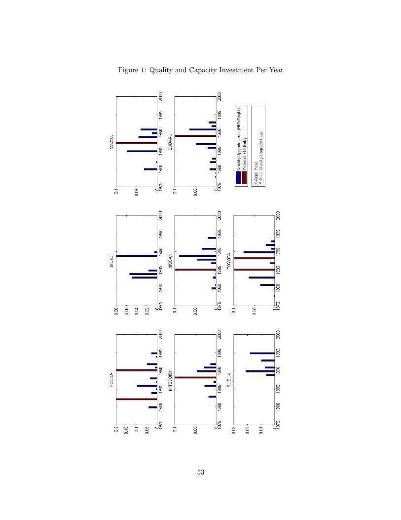
Figure 1: Quality and Capacity Investment Per Year
53

Figure 2: Difference Between Japanese Exports and VER Limits Per Year
54

Figure 3: Japan/U.S. Foreign Exchange Rates (Japanese Yen/U.S. Dollar)
Figure 4: Effect of VERs on Quality Investment
55

Figure 5: Effect of VERs on Capacity Investment with Dollar Depreciation
Figure 6: Effect of VERs on Capacity Investment without Dollar Depreciation
56

Figure 7: Effect of Capacity Investment Restriction on Quality Investment Policy
Figure 8: Effect of Quality Investment Restriction on Capacity Investment Policy
57
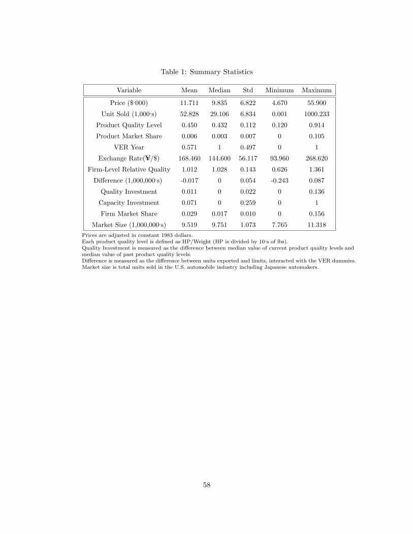
Table 1: Summary Statistics
Variable Mean Median Std Minimum Maximum
Price ($,000) 11.711 9.835 6.822 4.670 55.900
Unit Sold (1,000,s) 52.828 29.106 6.834 0.001 1000.233
Product Quality Level 0.450 0.432 0.112 0.120 0.914
Product Market Share 0.006 0.003 0.007 0 0.105
VER Year 0.571 1 0.497 0 1
Exchange Rate(¥/$) 168.460 144.600 56.117 93.960 268.620
Firm-Level Relative Quality 1.012 1.028 0.143 0.626 1.361
Difference (1,000,000,s) -0.017 0 0.054 -0.243 0.087
Quality Investment 0.011 0 0.022 0 0.136
Capacity Investment 0.071 0 0.259 0 1
Firm Market Share 0.029 0.017 0.010 0 0.156
Market Size (1,000,000,s) 9.519 9.751 1.073 7.765 11.318
Prices are adjusted in constant 1983 dollars.Each product quality level is defined as HP/Weight (HP is divided by 10,s of lbs).Quality Investment is measured as the difference between median value of current product quality levels andmedian value of past product quality levels.Difference is measured as the difference between units exported and limits, interacted with the VER dummies.Market size is total units sold in the U.S. automobile industry including Japanese automakers.
58

Table 2: Demand Estimates
Dependent Variable: ln(Annual Firm Market Share)-ln(Annual Outside Market Share)
Variable Coefficient Standard Error
Constant -0.951 0.260
ln(Price) 0.793 0.085
ln(Quality) 0.822 0.214
Firm (Brand) Fixed Effects Yes
Adjusted R-Squared 0.7001
Number of Observations 2012
Table 3: Effect of Firm’s State Variables on Annual Market Profit
Dependent Variable: Annual Market Profit in Billions of 1983 Dollars
Variable Coefficient Standard Error
Constant 1.141 1.324
Time Trend -0.020 0.013
VER Dummy -0.093 0.062
Lag FDI 0.329 0.079
Lag Quality-Upgrade 0.025 0.006
ln(Exchange Rate) 0.417 0.232
Relative Quality 1.603 0.196
Difference 1.988 1.030
Difference2 -16.091 6.288
Lag FDI·Relative Quality -0.041 0.079
Firm Fixed Effects Yes
Adjusted R-Squared 0.743
Number of Observations 140
59

Table 4: Effect of State Variables on Quality Investment
Dependent Variable: Annual Quality Investment Level
Variable Coefficient Standard Error
Constant 0.186 0.104
Time Trend -0.003 0.010
VER Dummy 0.006 0.012
Lag FDI -0.021 0.012
Lag Quality-Upgrade -0.002 0.004
ln(Exchange Rate) -0.016 0.018
Relative Quality -0.101 0.022
Difference 0.139 0.075
Difference2 0.920 0.455
Relative Quality·VER Dummy 0.027 0.013
Firm Fixed Effects Yes
Adjusted R-Squared 0.544
Number of Observations 132
Table 5: Effect of State Variables on Capacity Investment (Probit)
Dependent Variable: Annual Capacity Investment in the U.S. Dummy
Variable Coefficient Standard Error
Constant 24.203 12.681
Time Trend -0.215 0.161
VER Dummy 2.376 0.916
Lag FDI -0.201 0.884
Lag Quality-Upgrade -0.105 0.502
ln(Exchange Rate) -5.581 2.301
Relative Quality 3.419 2.254
Difference 47.600 21.587
Difference2 854.166 479.880
Firm Fixed Effects Yes
Prob>χ2 0.288
Number of Observations 132
60

Table 6: VERs Transition (Probit)
Dependent Variable: Annual VER Dummy
Variable Coefficient Standard Error
Constant -1.150 0.568
Lag VER Dummy 2.486 0.776
Prob>χ2 0.003
Observation 20
Table 7: Exchange Rate Transition
Dependent Variable: ln(Annual Japan/U.S. Foreign Exchange Rate)
Variable Coefficient Standard Error
Constant 0.352 0.438
ln(Lag Exchange Rate) 0.922 0.085
Adjusted R-Squared 0.866
Observation 20
Table 8: Relative Quality Transition
Dependent Variable: Annual Relative Quality
Variable Coefficient Standard Error
Constant 0.149 0.047
Lag Relative Quality 0.832 0.294
Quality Investment 2.138 0.294
Capacity Investment -0.009 0.026
Number of Observations 132
61

Table 9: Difference between Exports and VER Limits Transition
Dependent Variable: Annual Difference between Exports and VER limits
Variable Coefficient Standard Error
Constant -0.001 0.001
Lag Difference 0.608 0.067
Quality Investment -0.434 0.165
Capacity Investment -0.021 0.011
Number of Observations 132
Table 10: Dynamic Parameters
Variable Coefficient
Quality Investment Cost 1.856
Capacity Investment Cost 4.779
Standard Error of Quality Cost Shock 0.001
I simulate 1000 times and averaged to obtain expected values.Each simulation path has 100 year lifetimes.
62

Table 11: Average Quality-Upgrade levels with and without VERs
Average Quality-Upgrade Level
VERs 0.0014
No VERs 0.0007
Table 12: Average Probabilities of FDI with and without VERs (Dollar Depreciation)
Average Probability of FDI
VERs (Dollar Depreciation) 0.267
No VERs (Dollar Depreciation) 0.127
Table 13: Average Probabilities of FDI with and without VERs (No Dollar Depreciation)
Average Probability of FDI
VERs (No Dollar Depreciation) 0.267
No VERs (No Dollar Depreciation) 0.002
Table 14: Average Quality-Upgrade levels with and without FDI
Average Quality-Upgrade Level
FDI 0.0014
No FDI 0.0032
Table 15 Average Probabilities of FDI with and without Quality-Upgrade
Average Probability of FDI
Quality-Upgrade 0.369
No Quality-Upgrade 0.410
63


