R. & M. No. 3541
MINISTRY OF TECHNOLOGY
AERONAUTICAL RESEARCH COUNCIL REPORTS AND MEMORANDA
Investigations on an Experimental Single-stage
Turbine of Conservative Design
Part I A Rational Aerodynamic Design Procedure
Part II
By D. J. L. Smith and I. H. Johnston
Test Performance of Design Configuration
By D. J. L. Smith and D. J. Fullbrook
LONDON: HER MAJESTY'S STATIONERY OFFICE 1968
PRICE £1 l ls. 6d. NET
Investigations on
Turbine
an Experimental Single-stage of Conservative Design
Reports and Memoranda No. 3541"
January, 1967
Part I - - A Rational Aerodynamic Design Procedure
By D. J. L. Smith and I. H. Johnston
Summary. 'The design of a turbine stage is described in which all leading parameters (stage loading, flow coefficient,
pitch/chord ratio, blade profile shape and aspect ratio) have been selected conservatively to accord with current ideas for ensuring a reasonably high level of aerodynamic efficiency.
From consideration of the influence of stage loading KpAT V~ U,2 , flow coefficient ~ and rotor exit
swirl angle c~ 3, the stage design was selected such that these parameters were 1.15, 0.65 and 10 degrees
respectively. At the design speed of U ~ = 34 the resulting stage pressure ratio is approximately 1.65.
Such a stage duty is 'light' by aero engine standards but very comparable to much industrial gas turbine design practice.
Blade spacing and profile shapes are 'finally selected in such a way as to preclude severe opposing pressure gradients on the suction surface which might result in local separation of the boundary layer from the blade surfaces.
The methods applied and described for predicting blade surface velocities are simple and approximate only, and might readily be imitated by designers not wishing or able to exploit more elaborate and complex digital techniques.
*Part I replaces N.G.T.E.R.283--A.R.C. 28 614. Part II replaces N.G.T.E.R.292--A.R.C. 29 ¢~. ~ 7
Section
1. Introduction
2. Selection of Stage Parameters
.
CONTENTS
.
Initial Blade Design
3.1. Pitch/chord ratio
3.2. Blade number
3.3. Blade profile
4,1.
4.2.
Detailed Blade Design
Stator blade velocity distributions
Rotor blade velocity distributions
4.2.1. Mean diameter section
4.2.2. Outer diameter section
4.3. Final blade design
4.4. Comparison between two-dimensional and three-dimensional velocity distributions for the rotor blade
5. Conclusion
Acknowledgements
List of Symbols
References
Appendices I to VI
Tables 1 to 4
Illustrations--Figs. 1 to 26
Detachable Abstract Cards
LIST OF TABLES
N o . T i t l e
1 Blade section thickness distribution tmax/¢ = 10 per cent
2 Stator blade section co-ordinates
3 Rotor blade section co-ordinates
4 Final blade design parameters
LIST OF APPENDICES
N o . , T i t l e
I Construction of blade profile
II Blade surface velocities
III Radial equilibrium
IV Three-dimensional velocity distribution
V Stacking of blade sections
VI Blade stresses
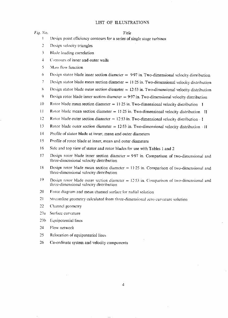
Fig. No.
I
,.)
3
4
5
6
7
8
9
10
ll
12
13
14
15
16
17
18
19
20
21
22
23a
23b
24
25
26
LIST OF I L L U S T R A T I O N S
Tit le
Design point efficiency contours for a series of single stage turbines
Design velocity triangles
Blade loading correlation
( 'ontours of inner and outer walls
Mass flow function
Design stator blade inner section diameter = 9.97 in. Two-dimensional velocity distribution
Design stator blade mean section diameter = 11.25 in. Two-dimensional velocity distribution
Design stator blade outer section diameter = 12.53 in. Two-dimensional velocity distribution
Design rotor blade inner section diameter = 9.97 in. Two-dimensional velocity distribution
Rotor blade mean section diameter = 11.25 in. Two-dimensional velocity distribution - !
Rotor blade mean section diameter = 11.25 in. Two-dimensional velocity distribution II
Rotor blade outer section diameter = 12.53 in. Two-dimensional velocity distribution+ !
Rotor blade outer section diameter = 12.53 in. Two-dimensional velocity distribution II
Profile of stator blade at inner, mean and outer diameters
Profile of rotor blade at inner, mean and outer diameters
Side and top view of stator and rotor blades for use with Tables 1 and 2
Design rotor blade inner section diameter = 9.97 in. Comparison of two-dimensional and three-dimensional velocity distribution
Design rotor blade mean section diameter = 11.25 in. Comparison of two-dimensional and three-dimensional velocity distribution
Desi~zn rotor blade outer section diameter = 12.53 in. Comparison of two-dimensional and three-dimensional velocity distribution
Force diagram and mean channel surface for radial solution
btrcamline geometry calculated from three-dimensional zero curvature solution
Channel geometry
Surface curvature
Equipotential lines
Flow network
Relocation of equipotential lines
Co-ordinate system and velocity components
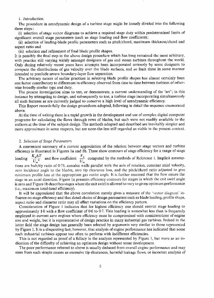
1. Introduction. The procedure in aerodynamic design of a turbine stage might be loosely divided into the following
three steps : (i) selection of stage vector diagrams to achieve a required stage duty within predetermined limits of
significant overall stage parameters (such as stage loading and flow coefficient); (ii) selection of leading-blade profile parameters such as pitch/chord, maximum thickness/chord and
aspect ratio and (iii) selection and refinement of final blade profile shapes.
It is possibly the final step in the above design procedure which has long remained the most arbitrary, with practice still varying widely amongst designers of gas and steam turbines throughout the world. Only during relatively recent years have attempts been incorporated seriously by some designers to compute the distributions of gas velocity over the blade surfaces, and so limit these in some manner intended to preclude severe boundary-layer flow separation.
The arbitrary nature of earlier practices in selecting blade profile shapes has almost certainly been one factor contributory to differences in efficiency observed from time to time between turbines of other- wise broadly similar type and duty.
The present investigation aims to test, or demonstrate, a current understanding of the 'art'; in this instance by attempting to design, and subsequently to test, a turbine stage incorporating simultaneously all such features as are currently judged to conserve a high level of aerodynamic efficiency.
This Report records fully the design procedures adopted, following in detail the sequence enumerated above.
At the time of writing there is a rapid growth in the development and use of complex digital computer programs for calculating the flows through rows of blades, but such were not readily available to the authors at the time of the subject design. The methods adopted and described are inevitably simpler and more approximate in some respects, but are none-the-less still regarded as viable in the present context.
2. Selection of Stage Parameters. A convenient summary of a current appreciation of the relation between stage vectors and turbine
efficiency is illustrated in Figures la and lb. These show contours of stage efficiency for a range of stage Va
loading KpAT and flow coefficient ~ computed by the methods of Reference 1. Implicit assump- Um 2
tions are hub/tip ratio of 0.75, annulus walls parallel with the axis of rotation, constant axial velocity, zero incidence angle to the blades, zero tip clearance loss, and the pitch/chord ratio adjusted to give minimum profile loss at the appropriate gas outlet angle. It is further assumed that the flow enters the stage in an axial direction. Figure la presents efficiency contours for stages in which the exit swirl angle is zero and Figure lb describes stages where the exit swirl is allowed to vary to given optimum performance (i.e., maximum total-head efficiency).
It will be appreciated that the above correlation merely gives a measure of the "vector diagram" in- fluence on stage efficiency and that detail choice of design parameters such as blade loading, profile shape, aspect ratio and diameter ratio may all effect variations on the efficiency pattern.
Consideration of Figure 1 indicates that for highest efficiency one should restrict stage loading to approximately 1-0 with a flow coefficient of 0.6 to 0-7. This loading is somewhat less than is frequently employed in current aero engines where efficiency must be compromised with considerations of engine size and weight, but it is representative of design practice in many industrial gas turbines. Indeed in the latter field the stage design has generally been selected by arguments very similar to those represented by Figure 1. It is a disquieting fact, however, that analysis of engine performance has indicated that some such industrial turbines appear too often to perform with indifferent efficiencies.
This is not regarded as proof of a fallacy in the analysis represented by Figure 1, but more as an in- dication of the difficulty of achieving an optimum design without some development.
The poor performance referred to above is usually deduced from overall engine performance and may stem from such simple causes as excessive tip clearances, harmful leakage flows, or incorrect analysis of
relative efficiencies of compressor and turbine components. Some efficiency penalty may however relate to the blade design in so far as the blade profiles may not be optimum for their aerodynamic duty.
Thus, although a stage loading of about 1-0 is an 'end point' in the range of aero engine turbines, it is of direct interest in the field of industrial turbine design.
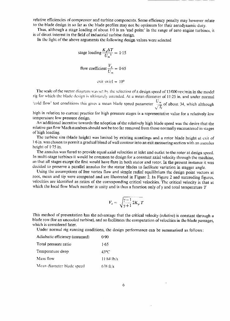
In the light of the above arguments the following design values were selected
KpA T stage loading 2 -- 1.15
U,,
flow coefficient - - = 0"65 Um
exit s~ill = 10 °
The scale of the vector diagram was set bx tile selection of a design speed of 13 000 rev/min in the model rig for which the blade design is ultimatel~ intended. At a mean diameter of 11-25 in. and under normal
"cold flow' test conditions this gives a mean blade speed parameter ~ of about 34, which although
high in relation to current practice for high pressure stages is a representative value for a relatively low temperature low pressure design.
Anadditional incentive towards the adoption of the relatively high blade speed was the desire that the relative gas flow Mach numbers should not be too far removed from those normally encountered in stages of high loading.
The turbine size (blade height) was limited by existing scantlings and a rotor blade height at exit of l '6 in. was chosen to permit a gradual blend of wall contour into an exit measuring section with an annulus height of 1'75 in.
The annulus was flared to provide equal axial velocities at inlet and outlet to the rotor at design speed. In multi-stage turbines it would be common to design for a constant axial velocity through the machine, so that all stages except the first would have flare in both stator and rotor. In the present instance it was decided to preserve a parallel annulus for the stator blades to facilitate variation in stagger angle.
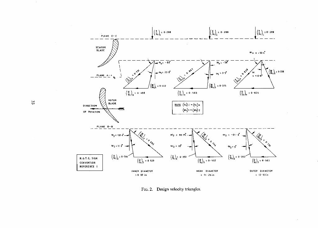
Using the assumptions of free vortex flow and simple radial equilibrium the design point vectors at root, mean and tip were computed and are illustrated in Figure 2. In Figure 2 and succeeding figures, velocities are identified as ratios of the corresponding critical velocities. The critical velocity is that at which the local flow Mach number is unity and is thus a function only of 7 and total temperature T
Vc = /Y-12Kp T "qT+ 1
This method of presentation has the advantage that the critical velocity (relative) is constant through a blade row (for an uncooled turbine), and so facilitates the computation of velocities in the blade passages, which is considered later.
Under normal rig running conditions, the design performance can be summarised as follows:
Adiabatic efficiency (assumed) 0.90
Total pressure ratio 1.65
Temperature drop 43oc
Mass flow 11-84 lb/s
Mean diameter blade speed 638 ft/s

Rotational speed 13 000 rev/min
Inlet total pressure 27.2 p.s.i, abs
Inlet total temperature 36G°K
Power 311 H.P.
Ratio of specific heats 1.4
3. Initial Blade Design. Having prescribed the design velocity vectors it was necessary to 'clothe' these with blades. The initial
approach used was that of selecting a design on a simple empirical basis as described in Sections 3.1 to 3.3.
3.1. Pitch/Chord Ratio. First consideration was given to the selection of stator and rotor pitch/chord ratio at mean diameter.
A criterion frequently adopted is the Zweifel 2 loading coefficient. This coefficient is defined as the ratio of the tangential lift of the real pressure distribution to an ideal one. The ideal pressure distribution has the maximum total pressure (inlet total assuming no losses) over the whole of the pressure surface the pressure falling instantaneously to the outlet static pressure P2 at the trailing edge. On the suction surface the pressure falls instantaneously to P2 at the leading edge and remains constant and equal to P2. The coefficient can be shown to be, for constant axial velocity,
~r = 2 S/C~ COS 2 0~ 2 (tan al -- tan az)
where al and a2 are the gas inlet and outlet angles (sign convention see Reference 1) and according to Zweifel should approximate to 0.8 to yield high blade efficiency. This deduction 2 was based on a limited number of steam turbine blade sections having high gas outlet angles. An attempt at a more general correlation is illustrated in Figure 3, where approximate optima of blade row loading coefficients (i.e., values yielding maximum efficiency) determined from miscellaneous cascade tests and turbine tests are shown plotted against gas outlet angle. The 'cascade' values in Figure 3 are derived from the analysis published in Reference 1, whilst the 'turbine' valfies are drawn from unpublished turbine tests in which the blade pitch/chord ratios were Varied to determine optimum blade numbers.
It is clear that although there is good agreement between gas turbine and cascade data at high outlet angles and the recommended value of 0.8, the optimum loading appears to increase as outlet angle is reduced. This trend is also indicated by the turbine test results which, however, require lower loading coefficients than the cascade results.
The loading coefficients selected for the stator* and rotor mean diameter sections were 0.76 and 0.85 respectively and it was originally intended that the axial chords would be maintained constant at all radii. However in order to minimise the radial variation of loading some variation in axial chord was accepted.
The values finally selected at this stage in the design are listed below
Diameter Inner
Loading coefficient 0.760 Pitch/axial chord 0.892
Stator
Mean I Outer
0.760 0.760 0.850 0.813
Rotor
Inner Mean Outer
0.885 0.850 0.815 0.760 0.946 1.150
*It should be noted that the axial velocity in fact increased through the stator blades.
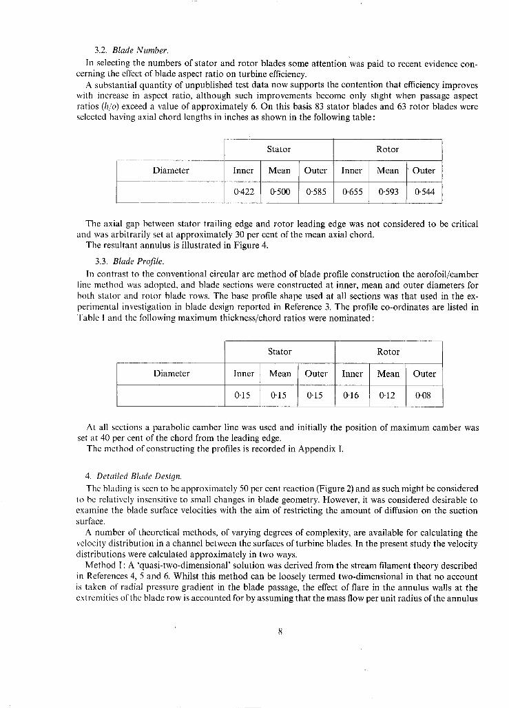
3.2. Blade Number.
In selecting the numbers of stator and rotor blades some attention was paid to recent evidence con- cerning the effect of blade aspect ratio on turbine efficiency.
A substantial quantity of unpublished test data now supports the contention that efficiency improves with increase in aspect ratio, although such improvements become only slight when passage aspect ratios (h/o) exceed a value of approximately 6. On this basis 83 stator blades and 63 rotor blades were selected having axial chord lengths in inches as shown in the following table :
Diameter
Stator
Inner Mean Outer
0.422 0-500 0.585
Inner
0.655
Rotor
Mean Outer
0.593 0.544
The axial gap between stator trailing edge and rotor leading edge was not considered to be critical and was arbitrarily set at approximately 30 per cent of the mean axial chord.
The resultant annulus is illustrated in Figure 4.
3.3. Blade Profile. In contrast to the conventional circular arc method of blade profile construction the aerofoil/camber
line method was adopted, and blade sections were constructed at inner, mean and outer diameters for both stator and rotor blade rows. The base profile shape used at all sections was that used in the ex- perimental investigation in blade design reported in Reference 3. The profile co-ordinates are listed in Table ! and the following maximum thickness/chord ratios were nominated :
Diameter
Stator
Inner Mean Outer
0.15 0.15 0.15
Rotor
Inner Mean Outer
0.16 0.12 0.08
At all sections a parabolic camber line was used and initially the position of maximum camber was set at 40 per cent of the chord from the leading edge.
The method of constructing the profiles is recorded in Appendix I.
4. Detailed Blade Design. The blading is seen to be approximately 50 per cent reaction (Figure 2) and as such might be considered
lo be relatively insensitive to small changes in blade geometry. However, it was considered desirable to examine the blade surface velocities with the aim of restricting the amount of diffusion on the suction surface.
A number of theoretical methods, of varying degrees of complexity, are available for calculating the velocity distribution in a channel between the surfaces of turbine blades. In the present study the velocity distributions were calculated approximately in two ways.
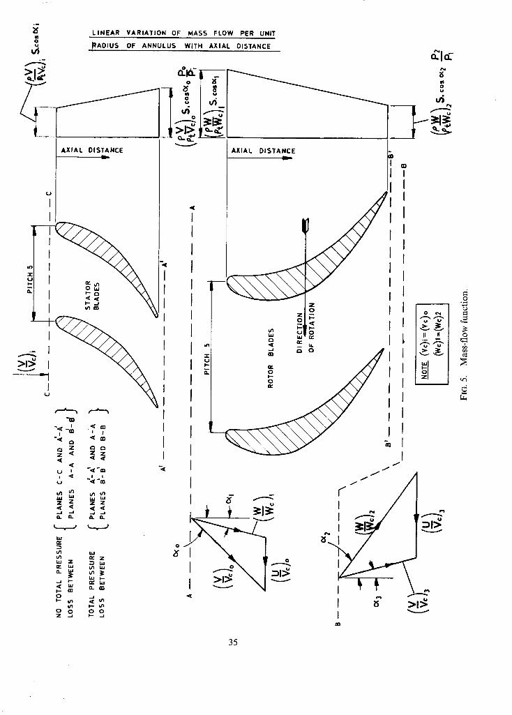
Method I : A 'quasi-two-dimensional' solution was derived from the stream filament theory described in References 4, 5 and 6. Whilst this method can be loosely termed two-dimensional in that no account is taken of radial pressure gradient in the blade passage, the effect of flare in the annulus walls at the extremities of the blade row is accounted for by assuming that the mass flow per unit radius of the annulus

passing through the blade channel decreases linearly from leading to trailing edges of blade (Figure 5) satisfying overall continuity at the inlet and outlet planes respectively. The numerical procedure is re- corded in Appendix II.
Method II : An approximate three-dimensional solution (derived from Reference 6), in which stream- line paths in the meridional plane have been determined in such a way as to satisfy more nearly the re- quirements of radial equilibrium of flow within the blade passage. The effect of this is to modify slightly the variation of mass flow per unit radius of annulus between inlet and outlet of the blade channels (at each respective radial station) from that more arbitrarily assumed in Method I. The development of the radial equilibrium equation and the numerical procedure for calculating the three-dimensional surface velocities are recorded in Appendices III and IV respectively.
The design of the blade sections described in Sections 4.1 to 4.3 is based wholly on Method I. Section 4.4 discusses the modifying effect on the surface velocity distributions resulting from use of the slightly more rigorous Method II; this effect is found, however, to be relatively small in the present design.
Each velocity distribution was assessed in relation to the NASA diffusion parameter 6, which, for the
maximum velocity- outlet velocity all velocities being relative to blade suction surface, is expressed as maximum relocit v '
the blade in question. Following the example of Reference 6 a diffusion parameter limit of 0.20 was specified and if this was
exceeded the blade section was modified. Where it was found necessary to re-design the section the thickness distribution was kept constant and either the position of maximum camber or the pitch/axial chord ratio was altered. The process is described more fully in the following sections.
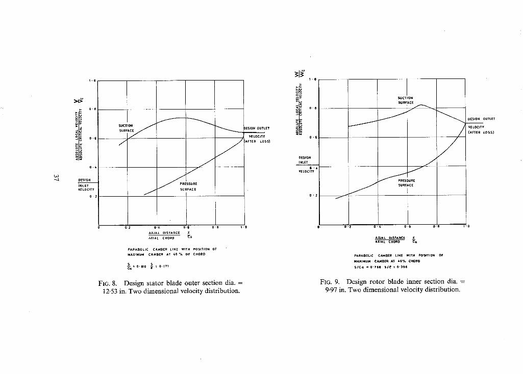
4.1. Stator Blade Velocity Distributions. The calculated surface velocities for the three stator blade sections are shown in Figures 6, 7 and 8,
as curves of absolute velocity V/Vc against axial position X/c,. Diffusion parameters for the inner, mean and outer diameter sections were 0.12, 0.07 and 0.14 re-
spectively. These were all well below the limiting value of 0.20, and it was realised that while there should be no risk of flow separation, the lift/drag ratio might be somewhat less than optimum. It was finally decided however to accept these sections, since this safety margin might be necessary to combat the influence of secondary flows.
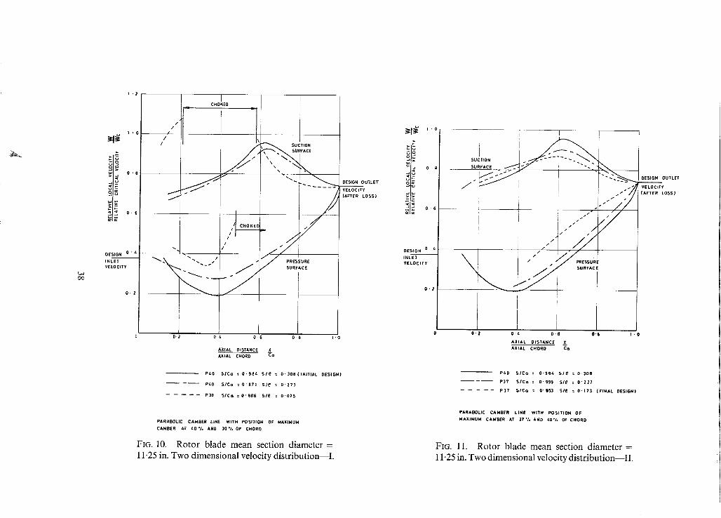
4.2. Rotor Blade Velocity Distributions. The calculated surface velocities for the three initial rotor blade sections are shown in Figures 9, 10
and 12, as curves of relative velocity W/Wc against axial position X/c,. Diffusion parameters for the inner, mean and outer diameter sections were 0.16, 0.23 and 0.25 respectively and of these only the inner diameter value was below the limiting value of 0.20. This section was therefore accepted without modifica- tion.
For the mean and outer sections, the maximum suction-surface velocity, on which the diffusion parameter depends, was found to occur near the throat. Equation (1) in Appendix II shows that the velocity is a function of the blade surface curvature. Therefore in order to reduce the diffusion parameter to an acceptable value these sections were modified so as to reduce the suction surface curvature in the region of the channel throat.
4.2.1. Mean diameter section. The Table below gives the suction surface curvature C s at the throat for the various modifications that were investigated and the calculated surface velocities are shown in Figures 10 and 11. C; and s/c'~ denote the initial values.
The pitch/axial chord ratio was altered by altering the axial chord.
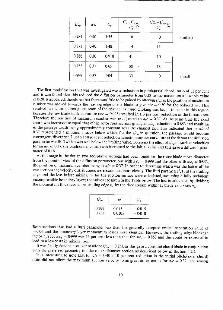
c~ S/C;--S/Ca% S/Ca
0.984
0.871
0'886
0.853
a/c
0.40
0.40
0"30
0.37
c~-c~_ % S/C'a
1.55 0 0
1.48 4 11
0"910 41 10
0.65 58 13
1.04 33 0
(initial)
(final)
The first modification that was investigated was a reduction in pitch/(axial chord) ratio of 11 per cent and it was found that this reduced the diffusion parameter from 0-23 to the maximum allowable value of 0-20. It appeared, therefore, that there was little to be gained by altering s/ca so the position of maximum camber was moved towards the leading edge of the blade to give a/c = 0'30 for the reduced s/c. This resulted in the throat being upstream of the channel exit and choking was found to occur in this region because the low blade back curvature (s/e = 0.025) resulted in a 3 per cent reduction in the throat area. Therefore the position of maximum camber was re-adjusted to a/c = 0.37. At the same time the axial chord was increased to equal that of the rotor root section, giving an s/c~ reduction to 0.853 and resulting in the passage width being approximately constant near the channel exit. This indicated that an a/c of 0.37 represented a minimum value below which, for the s/ca in question, the passage would become convergent/divergent. Due to a 58 per cent reduction in suction surface curvature at the throat the diffusion parameter was 0.13 which was well below the limiting value. To assess the effect of s/c,, on surface velocities for an a/c of 0"37, the pitch/(axial chord) was increased to the initial value and this gave a diffusion para- meter of 0.18.
At this stage in the design two acceptable sections had been found for the rotor blade mean diameter from the point of view of the diffusion parameter, one with s/ca = 0.999 and the other with s/ca = 0.853, the position of maximum camber being at a/c = 0.37. In order to determine which was the better of the two sections the velocity distributions were examined more closely. The Buri parameter 7, F, at the trailing edge and the loss before mixing, co, for the suction surface were calculated, assuming a fully turbulent incompressible boundary layer; the values are given in the Table below. The loss is calculated by dividing the momentum thickness at the trailing edge 0e by the 'free stream width' at blade exit, s.cos ~2.
s/ca co Fe
0-999 0-015 -0-015 0.853 0.0105 - 0-010
Both sections thus had a Buri parameter less than the generally accepted critical separation value of -0 .06 and the boundary layer momentum losses were identical. However, the trailing edge blockage factor te/s for s/c~ = 0"999 was 13 per cent less than that for s/c, = 0.853 and this could be expected to lead to a lower wake mixing loss.
It was finally decided ho~ ever to adopt s/ca = 0.853, as this gave a constant chord blade in conjunction with the preferred geometry for the outer diameter section as described below in Section 4.2.2.
It is interesting to note that for a/c = 0.40 a 10 per cent reduction in the initial pitch/(axial chord) ratio did not affect the maximum suction velocity to as great an extent as for a/c = 0.37. The reason
10

for this is that the suction surface curvature at the throat was only reduced by 4 per cent for a/c -- 0.40 whereas for a/c = 0.37 the reduction was 38 per cent.
4.2.2. Outer diameter section. The Table below gives the suction surface curvature Cs at the throat for the various modifications that were investigated and the calculated surface velocities are shown in Figures 12 and 13. Cs and s/c'a denote the initial values.
SIc a a/c
1.231 0-40
1.180 0.37
0.856 0.37
0.962 0.37
Cs
1"38
C'~-C~ /
Cs
0
- - % s/c;-s/e. % s/c;
0
1.060 23 4
0.525 62 30
0.699 49 22
(initial)
(final)
In view of the results from the mean section the first modification was a 4 per cent reduction in pitch/ axial chord and the position of maximum camber was moved towards the leading edge of the blade to give a/c = 0.37. However, the diffusion parameter was only reduced from 0.25 to 0.24, the maximum allowable value being 0.20. It was found for this section that in the region of the channel exit the passage width was approximately constant so in order to maintain a convergent passage the position of maximum camber could not be moved nearer to the leading edge of the blade. To assess the effect of pitch/axial chord on the surface velocities a major reduction in s/ca of 30 per cent for a/c = 0.37 was investigated. This resulted in a considerable reduction in the peak velocity due to a 62 per cent reduction in suction surface curvature at the throat and the diffusion parameter was reduced to 0.17. However. the axial chord required was 11 per cent greater than that for the inner section. As a final compromise the axial chord was made equal to that of the inner section to give a pitch/axial chord of 0.962, a reduction of 22 per cent from the initial value. This modification resulted in a diffusion parameter of 0.185 which
was considered acceptable. The outlet velocity used in assessing the diffusion parameter was the mean value allowing for the blade
pressure loss which was assumed to occur downstream of the trailing edge of the blade. In the NASA blade design study 6 however the outlet velocity just upstream of the trailing edge was used, with the loss assumed to occur downstream of this region. This velocity was computed in the same manner for the present case assuming no change in the tangential velocity and allowing for trailing edge blockage. The velocity ratio W/Wc was found to be 0.788 compared with the original value of 0.791, so it was evident that in this case the diffusion parameter was not sensitive to the alternative definition of outlet
velocity.
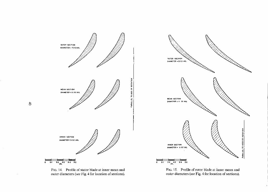
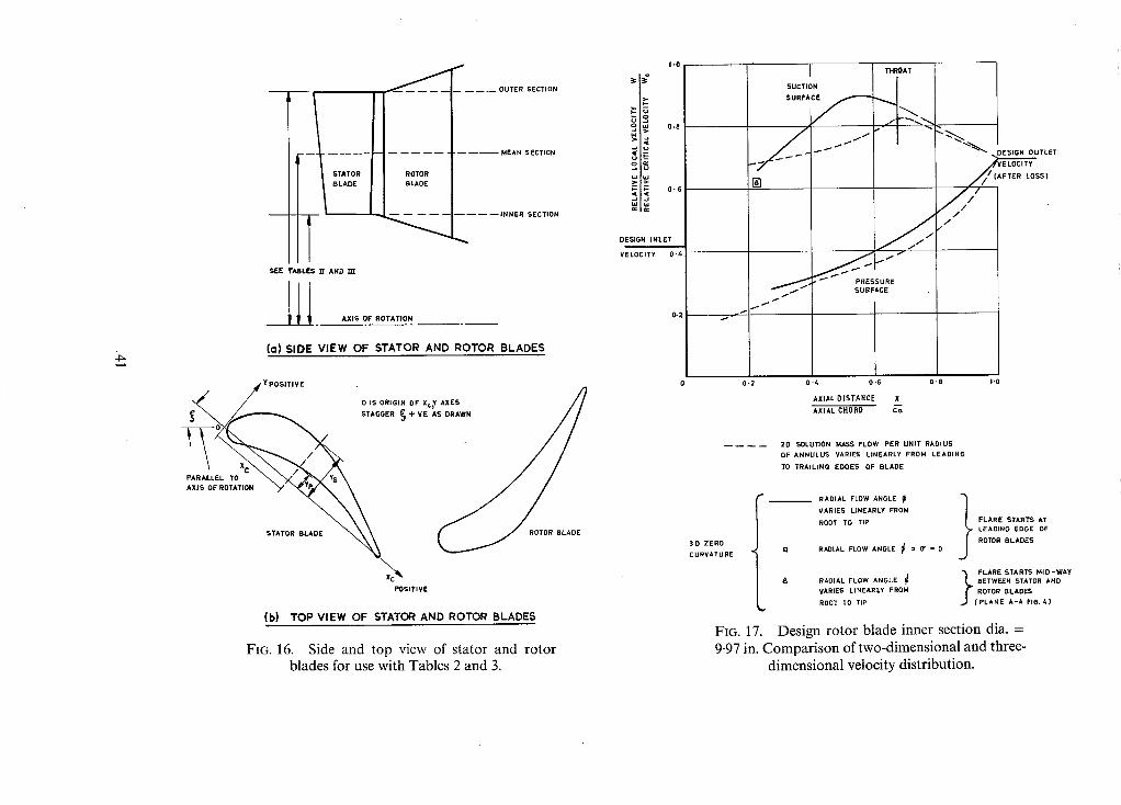
4.3. Final [31ade Design. The selected blade profiles are shown in Figures 14 and 15 and the blade co-ordinates are listed in
Tables 2 and 3 for the co-ordinate system illustrated in Figure 16. The stacking of the sections is described in Appendix V and the blade stresses are recorded in Appendix
VI. The principal design parameters finally selected for the various blade stations are recorded in Table 4.
4.4. Comparison between Two-Dimensional and Three-Dimensional Velocity Distributions for the Rotor Blade.
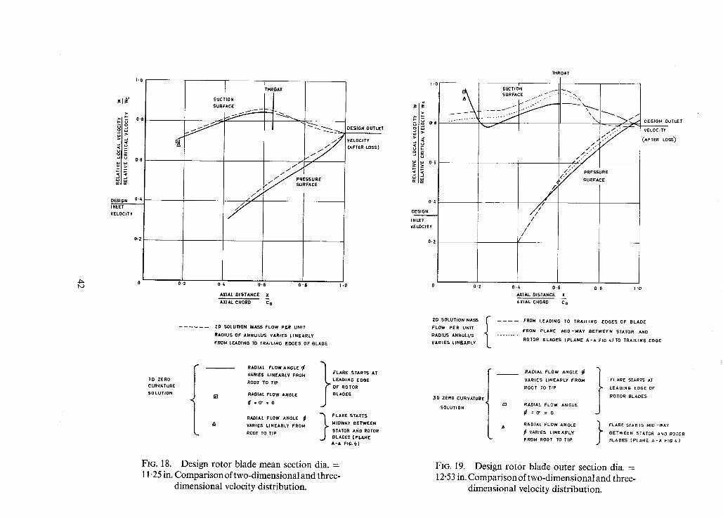
The calculated three-dimensional (neglecting streamline curvature in the meridional plane) and two- dimensional velocity distributions for the three design rotor blade sections, assuming no loss in total
11
pressure within the channel, are compared in Figures 17, 18 and 19. In the three-dimensional analysis the suction surface velocities in the region downstream of the throat were approximated by joining the throat velocity to that of the exit by a smooth curve.
In the two-dimensional analysis of velocity the mass flow per unit radius of the annulus was assumed to vary linearly with axial distance between the leading and trailing edges of the blade, Figure 5. The design inlet velocity triangles to the rotor blade were computed for a plane mid-way between the stator and rotor blades, Figure 2, so the surface velocities for the three rotor blade sections were reassessed allowing the mass flow to vary from this plane. As might be anticipated neither of the three sections were very sensitive to the inlet plane assumption and Figure 19 shows the velocity distribution for the outer diameter section which was most sensitive to this assumption.
From Figure 19 it may be seen that the three-dimensional solution shows a steep adverse velocity gradient for the suction surface near the leading edge of the outer section which was not apparent in the two-dimensional solution. It was thought that this may have been due to the assumptions made in the initial analysis of velocity regarding annulus flare and radial flow angle, which were,
(i) annulus flare starts at leading edge of rotor blades; (ii) radial flow angle q~ in the meridional plane varies linearly from inner to outer diameters. Therefore the surface velocities near the leading edge of the rotor blade were reassessed using two
alternative methods of calculation. In the first of these the radial flow angle was put equal to zero. For the second it was assumed that the annulus flare started midway between the stator trailing edge and rotor leading edge and the variation of radial flow angle was as in the initial method of calculation. Figures 17, 18 and 19 show that these alternative methods had little effect on the surface velocities near the leading edge.
Radial equilibrium was assumed to exist along a mean channel surface (Figure 20a) which is defined, at any radius, as being a smooth curve passing through the mid-points of the equipotential lines in the circumferential plane. The relative flow angle on this mean channel surface was determined by assuming a linear variation of flow angle along equipotential lines. The rotor outer section was set at a high stagger angle which resulted in a large variation of the relative flow angle along the circumferential equipotential lines near the channel entrance. It is believed that the adverse velocity gradient for the suction surface near the leading edge of the rotor outer section may be due to inaccuracies in the mean channel surface flow angle.
The rotor inner and outer sections show the most sensitivity to the type of flow assumption. The three- dimensional solution gave a velocity distribution of higher level than the two-dimensional solution for the inner section and of generally lower level for the outer section, the difference in the two solutions for mean section being very small. Also the location of the peak suction surface velocity is different, parti- cularly for the inner section. However, it must be pointed out that in the three-dimensional solution the streamline curvature in the meridional plane was neglected. Figure 21 shows the streamlines calculated from the three-dimensional solution and it may be seen that they have a definite curvature. Also shown are the streamlines for the two-dimensional solution; these are straight lines due to the assumptions made in this approach.
5. Conclusion. A rational approach to the design of a particular experimental turbine stage has been attempted and
described, the principal objective being to conserve a high level in stage aerodynamic efficiency. Con- sequent choices of basic vector diagrams, leading blade parameters and final refinements in blade profile shapes have each been described in detail.
The mean diameter velocity triangles were selected to give optimum efficiency conditions on the basis of current design data, those at other diameters being based on the assumptions of free vortex flow and simple radial equilibrium. The Mach numbers were comparable to those used in current aircraft
/KpAT\ engine practice, but the stage loading ~ - 2 ) was more representative of values used in industrial gas
turbines.
12

The blade geometry was initially chosen on the basis of empirical rules. Blade surface velocities were then assessed by means of a quasi-two-dimensional approach, and modifications were made so as to restrict the amount of diffusion on the suction surface to a limiting value.
The final design for the rotor blades was also examined using a modified method which additionally satisfied radial equilibrium in the blade passages. The results suggested somewhat increased surface velocities for the inner diameter section, and somewhat reduced values for the outer section, than were calculated in the design procedure. It was not considered justifiable, however, to make further changes to the design, in view of the many assumptions which had to be made in this approach.
Acknowledgements. The authors wish to express thanks to Miss J. Marshall for performing most of the calculations and
to Mr. F. Stokes for drawing and stressing the blade profiles.
13

C
Ds
E
H
I
J
Kp
L
M
P
T
AT
U
V
W
X,,, Y
x, y
X
a
b
¢
Cp
C v
d
e
9
h
i
J
k
m
LIST OF SYMBOLS
Blade surface curvature
Suction diffusion parameter, defined as maximum blade surface relative velocity - blade outlet relative velocity
maximum blade surface relative velocity
Length of circumferential equipotential lines
Total enthalpy = 9JcpT
Modified total enthalpy = H-co(Vwr )
Mechanical equivalent of heat
Specific heat at constant pressure = 9Jcp
Distance along blade surface from leading edge stagnation point
Mach number
Total pressure
Total temperature
Stage temperature drop
Blade speed
Absolute gas velocity
relative gas velocity
Rectangular cartesian co-ordinates defining point on the blade
Surface
Axial distance measured from leading edge of blade
Distance of point of maximum blade camber from leading edge
Maximum blade camber
Blade chord
Specific heat at constant pressure
Specific heat at constant volume
Length of camber line (Table 1)
Blade back curvature
Acceleration due to gravity
Static enthalpy, or blade height
Gas incidence angle on blade
Length used in defining blade back curvature (Appendix I)
Tip clearance
Mass flow per unit radius expressed semi-non-dimensionally by dividing by ptWc
Distance along circumferential equipotential lines measured from suction surface
14
o
P
r
s
t
u
y'
y "
~x
z
7
0
P
¢
o)
f f
0
OT F
1J
Subscripts. a
c
ci
e
h
i
m
max
LIST OF SYMBOLS--(contd.)
Blade opening (throat)
Static pressure
Radius about axis of rotation or radius of curvature of streamlines in circumferential plane
Blade pitch or entropy
Absolute static temperature or blade thickness or time
Internal energy
Slope of blade surface
Rate of change of slope of blade surface
Spacing between (y) ordinates
Distance in axial direction or length used. in defining blade back curvature (Appendix I)
Absolute gas flow angle measured from axial direction
Relative gas flow angle measured from axial direction or blade inlet angle measured from axial direction
Ratio of specific heats
Boundary layer momentum thickness or angular co-ordinate or blade camber angle
Gas density
Blade stagger angle measured from axial direction
Mass average pressure-loss coefficient or rotational speed
Blade camber inlet or outlet angle
Radial flow angle in mean channel surface
Radial flow angle in meridionial plane or velocity potential expressed semi-non-dimen- sionally by dividing by W~
Stream function
Zweifel loading coefficient
Buri parameter
Kinematic viscosity
Axial component
Critical conditions i.e. corresponding to a local Mach number of 1-0 (see Appendix II)
Resultant velocity in circumferential plane
Trailing edge
Hub conditions
Absolute stator inlet conditions
Resultant velocity in meridional plane and mean diameter conditions
Maximum
15
mid
m s
P /.
S
t
W
0
1
2
3
LIST OF SYMBOLS---(contd.)
Conditions at mid-streamline in circumferential plane
Mean channel surface
Pressure surface
Radial component
Suction surface
Total head conditions
Whirl component
Absolute stator outlet conditions
Relative rotor inlet conditions
Relative rotor outlet conditions
Absolute rotor outlet conditions
16

No. Author(s)
i D.G. Ainley and G. C. R. Mathieson
2 O. Zweifel . . . .
3 I.H. Johnston and .. D. E. Smart
4 A. Stodola . . . .
5 M.C. Huppart . . . . C. MacGregor . . . . . .
6 J.W. Miser and W. L. Stewart
A. Buri . . . . . . . . (Translated from the German by M. Flint)
7
REFERENCES
Title, etc.
A method of performance estimation for axial flow turbines. A.R.C. & M. 2974, December 1951.
The spacing of turbo-machine blading especially with large an- gular deflecting.
The Brown Boveri Review Vol. 32, No. 12, 1945.
An experiment in turbine blade profile design. A.R.C.C.P.941, October 1965.
Steam and gas turbines, Vol. II. McGraw-Hill Book. Co. Inc. 1927, p. 992, (Reprinted, Peter Smith (New York) 1945).
Comparison between predicted and observed performance of gas turbine stator blade designed for free vortex flow.
NACA TN.1810, April 1949.
Investigation of two-stage air-cooled turbine suitable for flight Mach number of 2.5-II-blade design.
NACA RM. E56K06, January 1957. T.I.L. No. 5396.
A method of calculation for the turbulent boundary layer with accelerated and retarded basic flow.
R.T.P. Trans. No. 2073. Issued by the Ministry of Aircraft Pro- duction.
8 R.V. Southwell
9 W.J. Whitney ..
10 Chuang-Hua Wu
•. Relaxation methods in theoretical physics• Oxford University Press, 1946.
Tabulation of mass-flow parameters for use in design of turbo- machine blade rows for ratios of specific heats of 1.3 and 1.4.
NACA TN.3831 October, 1956.
A general theory of three-dimensional flow in subsonic and supersonic turbo-machines of axial- radial- and mixed-flow types.
NACA TN.2604, January 1952.
17

APPENDIX I
Construction of Blade Profile. Assumptions. (i) The camber line is parabolic. (ii) The rotor blades have a finite radial tip clearance of k/h = 0.006 where h is the mean blade height. (iii) Gas outlet angle correction for the rotor blades, due to the finite radial tip clearance, varies
linearly from root to tip, being zero at the root diameter.
Numerical procedure. Let suffix 1 denote inlet and 2 outlet from the blade. The sign convention for the gas and blade angles
is given in Reference 1. The numerical procedure is as follows: 1. The camber outlet angle is given by
4 b/c tan Zz = 3 - 4 a/c
where
4 tan 1 (;i1 +,4 3 t l - 0
and a_ = position of maximum camber, as a fraction of the chord, measured from the leading edge of the C
a blade. As a first approximation a s sume- = 0.4, which may be altered after calculating the surface
c velocity distribution, (see Section 4). Assume blade camber angle = gas inlet ang le -gas outlet angle, i.e., 0 = czl- ~2.
2. The camber inlet angle Xl and stagger angle ~ are given by
Zl = O-Z2
= Zl-3i
as a first approximation assume/~1 = el-
3. Assuming the axial chord (Section 3.2) to be equal to the axial distance between the points of intersection of the camber line with the blade profile at the leading and trailing edges of the blade then the chord c' is given by
C I _ Ca
COS ~ "
4. Having calculated the chord c', the leading and trailing edge radii and thickness distribution can be found using Table 1. It is assumed that c' = true chord c.
With the blade pitch s known, the channel can be constructed and the opening o measured. The blade back curvature e is given by
j2
e = 8zz (Figure 3 of Reference 1)
18
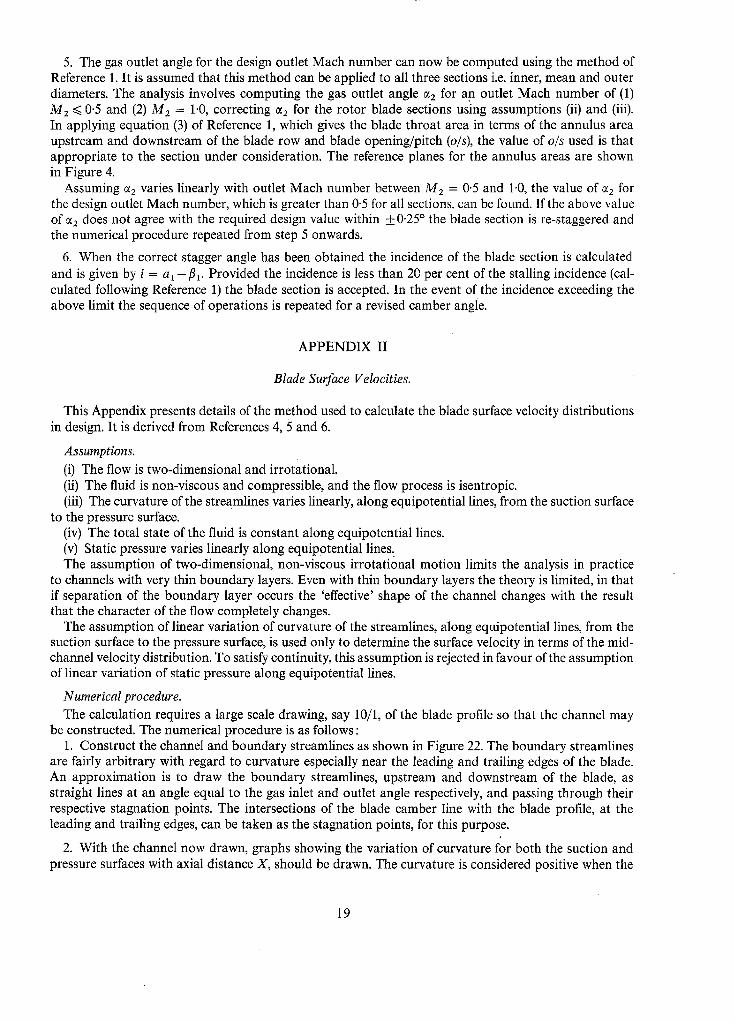
5. The gas outlet angle for the design outlet Mach number can now be computed using the method of Reference 1. It is assumed that this method can be applied to all three sections i.e. inner, mean and outer diameters. The analysis involves computing the gas outlet angle e2 for an outlet Mach number of (1) ME ~< 0-5 and (2) M2 = 1.0, correcting ea for the rotor blade sections using assumptions (ii) and (iii). In applying equation (3) of Reference 1, which gives the blade throat area in terms of the annulus area upstream and downstream of the blade row and blade opening/pitch (o/s), the value of o/s used is that appropriate to the section under consideration. The reference planes for the annulus areas are shown in Figure 4.
Assuming c~ 2 varies linearly with outlet Mach number between M2 = 0.5 and 1.0, the value of c~ z for the design outlet Mach number, which is greater than 0.5 for all sections, can be found. If the above value of e2 does not agree with the required design value within __+ 0.25 ° the blade section is re-staggered and the numerical procedure repeated from step 5 onwards.
6. When the correct stagger angle has been obtained the incidence of the blade section is calculated and is given by i = al - i l l . Provided the incidence is less than 20 per cent of the stalling incidence (cal- culated following Reference 1) the blade section is accepted. In the event of the incidence exceeding the above limit the sequence of operations is repeated for a revised camber angle.
APPENDIX II
Blade Surface Velocities.
This Appendix presents details of the method used to calculate the blade surface velocity distributions in design. It is derived from References 4, 5 and 6.
Assumptions. (i) The flow is two-dimensional and irrotational. (ii) The fluid is non-viscous and compressible, and the flow process is isentropic. (iii) The curvature of the streamlines varies linearly, along equipotential lines, from the suction surface
to the pressure surface. (iv) The total state of the fluid is constant along equipotential lines. (v) Static pressure varies linearly along equipotential lines. The assumption of two-dimensional, non-viscous irrotati0nal motion limits the analysis in practice
to channels with very thin boundary layers. Even with thin boundary layers the theory is limited, in that if separation of the boundary layer occurs the 'effective' shape of the channel changes with the result that the character of the flow completely changes.
The assumption of linear variation of curvature of the streamlines, along equipotential lines, from the suction surface to the pressure surface, is used only to determine the surface velocity in terms of the mid- channel velocity distribution. To satisfy continuity, this assumption is rejected in favour of the assumption of linear variation of static pressure along equipotential lines.
Numerical procedure. The calculation requires a large scale drawing, say 10/1, of the blade profile so that the channel may
be constructed. The numerical procedure is as follows : 1. Construct the channel and boundary streamlines as shown in Figure 22. The boundary streamlines
are fairly arbitrary with regard to curvature especially near the leading and trailing edges of the blade. An approximation is to draw the boundary streamlines, upstream and downstream of the blade, as straight lines at an angle equal to the gas inlet and outlet angle respectively, and passing through their respective stagnation points. The intersections of the blade camber line with the blade profile, at the leading and trailing edges, can be taken as the stagnation points, for this purpose.
2. With the channel now drawn, graphs showing the variation of curvature for both the suction and pressure surfaces with axial distance X, should be drawn. The curvature is considered positive when the
19
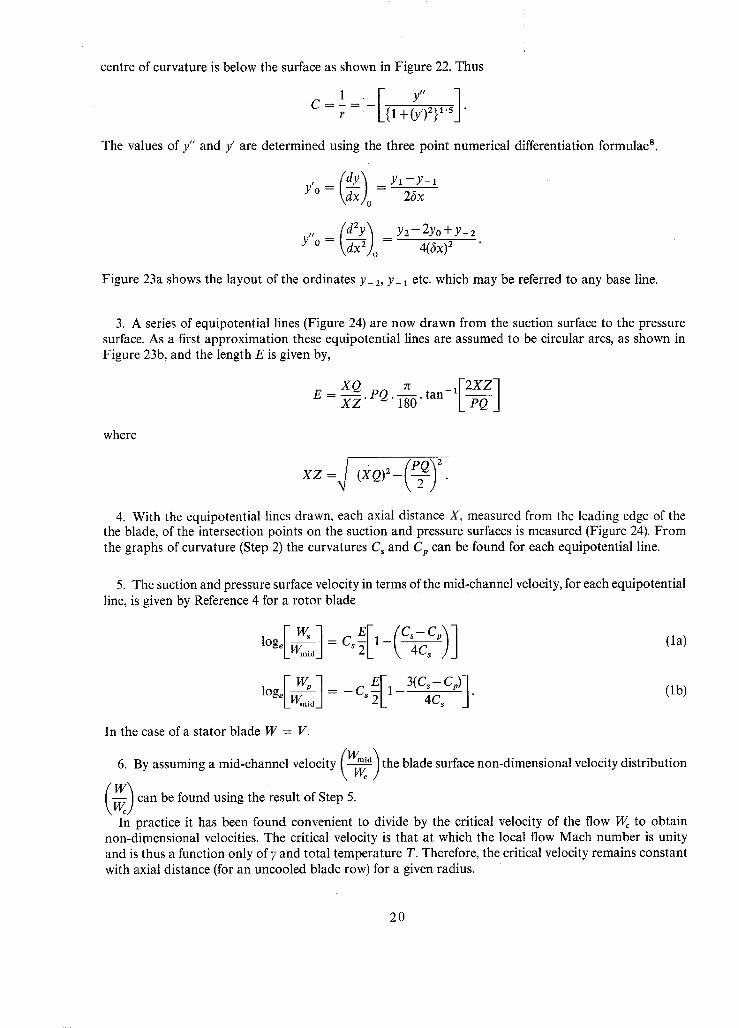
centre of curvature is below the surface as shown in Figure 22. Thus
1 . V . y" -] r L{1 +(.,v')2}l'~J"
The values of y" and y' are determined using the three point numerical differentiation formulae s.
(d )o Y'o = = 26x
Y"o ( d 2 y ) y2-2yo+Y-2 = \~X2)o = 4(ax)2
Figure 23a shows the layout of the ordinates y_ 2, Y- 1 etc. which may be referred to any base line.
3. A series of equipotential lines (Figure 24) are now drawn from the suction surface to the pressure surface. As a first approximation these equipotential lines are assumed to be circular arcs, as shown in Figure 23b, and the length E is given by,
rc f 2 X Z-] XQ pQ -i-8-6 " tan- L-P-Q-J E = X Z " "
where
4. With the equipotential lines drawn, each axial distance X, measured from the leading edge of the the blade, of the intersection points on the suction and pressure surfaces is measured (Figure 24). From the graphs of curvature (Step 2) the curvatures Cs and Cp can be found for each equipotential line.
5. The suction and pressure surface velocity in terms of the mid-channel velocity, for each equipotential line, is given by Reference 4 for a rotor blade
= logf l c, LWmd 2L \ 4c~ ) J
(la)
1oge[wW~Pe] = - -c~E[ 1 3(Cs-CP)]~ ] ' (lb)
In the case of a stator blade W = V.
6. By assuming a mid-channel velocity ~ the blade surface non-dimensional velocity distribution
(~-~) can be found using the result of Step 5.
In practice it has been found convenient to divide by the critical velocity of the flow W~ to obtain non-dimensional velocities. The critical velocity is that at which the local flow Mach number is unity and is thus a function only of V and total temperature T. Therefore, the critical velocity remains constant with axial distance (for an uncooled blade row) for a given radius.
20

W~ VVp obtained, the integrated mass flow across each equipotential line 7. With the values of E, ~ and
can be determined. The equation of continuity gives :
or for convenience n
m - E~ -i=1"° p--W p, VV~d(E ) (2) - jn_= ° p,W~
E Equation (2) is solved by using the tables and method of integration given in Reference 9. The correct mid-channel velocity distribution (Step 6) has been assumed when the integrated mass flow equals the specified mass flow. The specified mass flow per unit radius of the annulus was assumed to vary linearly with axial distance between the leading and trailing edges as shown in Figure 5. Ideally then, the integrated mass flow given by Equation (1) should equal the specified mass flow but an error of not more than I per cent is usually acceptable.
W. 8. Having satisfied continuity the surface velocity distribution - - is known and can be plotted against
blade surface length L measured from the leading edge stagnation point. The suction surface velocities in the region 4a to the trailing edge stagnation point and 48 to the leading edge stagnation point (Figure 24) are only approximate because the channel is bounded by assumed streamlines in these regions.
9. With the surface velocity distribution obtained, the flow network (Figure 24) can be checked. The velocity potential 4 is given by
4 = f w d L
where L is the distance measured along blade surface from leading edge stagnation point, or for con- venience
The accuracy of the network from ¢8 to the leading edge and 43 to the trailing edge cannot be checked since the velocity distribution for the suction surface in these regions is only approximate. Since the absolute value of 4 is arbitrary the value of 43, the velocity potential at the channel throat, is set equal to zero on both the suction i~nd pressure surfaces. To solve equation (3) it is assumed that the curve of W
- - versus L (Step 8) varies linearly between adjacent points and the elemental velocity potential between
two L points is given by
A 4 = ½ + ~ L - L b (4) a
where stations a and b correspond to adjacent equipotential lines. The integration is carried out from the channel throat towards the leading edge stagnation point for
both the suction and pressure surfaces. By adding the A 4 values the value of
W ¢ = : d L = a ¢
L t h r o a t L t h r o a t
21

can be found at each L point, for both the suction and pressure surfaces. A graph is now drawn showing the variation of ~b with L for both surfaces (Figure 25). For irrotational motion the line integral of velocity around any closed path in the field of flow must be equal to zero. Hence,
4~n ~n
~3 ~3
(5)
where n = 4, 5, 6 - (Figure 24). Therefore it is seen from equation (5) that by fixing the position of the equipotential lines on one surface
of the blade their position on the other surface can easily be found. Figure 25 shows the relocation of the equipotential lines on the suction surface, fixing their position on the pressure surface. Having relocated the equipotential lines, the surface velocities may be recomputed.
Experience shows that in many cases the initial selection of the potential network is sufficiently accurate for this iteration to be superfluous.
APPENDIX III
Radial Equilibrium.
This Appendix presents the development of the equation for radial equilibrium.
Assumptions.
(i) The flow is non-viscous and compressible. (ii) Steady axially symmetric flow is assumed to exist throughout the turbine annulus. (iii) The surfaces of the blades are approximately radial so that radial blade force can be neglected. (iv) The blades have zero tip clearance.
General equation.
The co-ordinate system and velocity components are shown in Figure 26. The forces acting in the radial direction are the centrifugal force due to the absolute whirl velocity and an acceleration force due to the variation in radial velocity, Figure 20a (both positive as drawn). The radial velocity is taken to be positive when outwards from the axis of rotation, i.e. the radial flow angle ~b in the meridional plane and a in the plane containing the relative velocity W, Figure 26, are positive when the curvature of the streamline is outward from the axis of rotation. Equating the sum of the force components to the radial pressure gradient
g Op Vw 2 DV~ p & r Dt (6)
O . where Dt is the operator following the motion.
From assumption (ii) it follows that
DV, ~ ~V~ Dt - Vr +V, 0~" (7)
Combining equations (6) and (7) we get
g @ p Fr
OV~ Vw 2 - - V r ~ - V a x •
r Cr ( ' z (8)
22
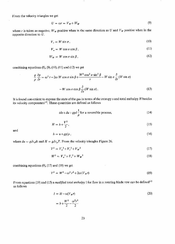
From the velocity triangles we get
U = mr = V w + W w (9)
where r is taken as negative, Ww positive when in the same direction as U and Vw positive when in the opposite direction to U.
Vr = W sin or, (10)
V, = W cos ~ cos fl, (11)
Ww = W cos cr sin fl, (12)
combining equations (8), (9), (10), (11) and (12) we get
g 0 p __ (.02 r - - 2¢o W c o s ~ sin fl q p Or
W 2 COS 2 O" s i n 2 fl r
W sin a - - (W sin a) &
- W cos o" cos fl ~z (W sin a). (13)
It is found convenient to express the state of the gas in terms of the entropy s and total enthalpy H besides its velocity components 1°. These quantities are defined as follows
1 tds + du + gpd - ' for a reversible process,
P (14)
and
V 2 H = h + - - (15)
2 '
h = u+gp/p , (16)
where du = gJcvdt and H = gJcvT. From the velocity triangles Figure 26.
V 2 = V. 2+Vr 2+VW 2 (17)
W 2 = V. 2+V~ 2+WW 2 (18)
combining equations (9), (17) and (18) we get
V 2 = W2-a~ 2 r2+20~(Vw r) (19)
From equations (19) and (15) a modified total enthalpy I for flow in a rotating blade row can be defined 1° as follows
I = H - oJ(Vwr) (20)
W 2 (.02/,2 = h + - -
2 2
23

From equations (14) and (16) we get
dh = 9_ dp + tds P
(21)
From equations (20) and (21),
OI 9 8p 8s OW OH O(Vwr) - + t ~ + W T r - r - ~ ° 2 r =-~r -°~ ar Or p Or (22)
0W Combining equations (13) and (22), dividing through by W z cos / a and combining terms in ~ we get
upon integrating
i cos ] + S i fl 2o) sinfl 1 8I lOge W h COS ~7 h rh W COS O" W 2 c o s 2 O" O--r
t Os 0a t a n a c o s f l 8W] W 2 c o s 2 (7 0 r - c o s fl Oz W ~z dr = 0 (23)
where suffix h denotes Col~ditions at the hub diameter.
Simple radial equilibrium.
The simplest solution of the radial equilibrium equation is arrived at by assuming 1° (a) the blade rows are not placed too closely together (b) the gas enters the turbine with uniform enthalpy H and entropy s and zero vorticity (c) the flow is adiabatic (or from assumption (i) and equation (14) is isentropic) i.e. the entropy is
constant
(d) the blades impart a radial variation of tangential velocity in a plane downstream of the blades which is inversely proportional to the radius i.e. Vwr = constant
(e) the curvature of the streamlines is small and can be neglected. The resulting equation is, from (22), for a rotor blade
I W c o s a q Ir[-sin/f l 2o)sinfl 1 - + - - d r = 0 (24 )
l o g , Wh COS O'h_ ] 3..L r W cos
For a stator blade e) = 0 and W = V.
APPENDIX IV
Three-Dimensional Velocity Distribution.
This Appendix presents the numerical procedure in calculating the three-dimensional velocity dis- tribution for the rotor blade sections, neglecting streamline curvature. The main approximation is in assuming that radial equilibrium exists along a mean channel surface. The mean channel surface, Figure 20b, is defined, at any radius, as being a smooth curve passing through the mid-points of the equipotential lines in the circumferential plane, which is the definition used by NASA 6.
The calculation does not require the mean channel surface to be composed of streamlines since the mass flow between it and the suction and pressure surfaces can vary from one axial station to the next. It is only assumed that at a given axial station, measured on the mean channel surface, Figure 20, the
24
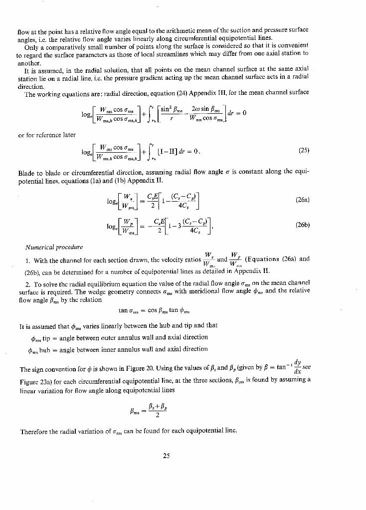
flow at the point has a relative flow angle equal to the arithmetic mean of the suction and pressure surface angles, i.e. the relative flow angle varies linearly along circumferential equipotential lines.
Only a comparatively small number of points along the surface is considered so that it is convenient to regard the surface parameters as those of local streamlines which may differ from one axial station to another.
It is assumed, in the radial solution, that all points on the mean channel surface at the same axial station lie on a radial line, i.e. the pressure gradient acting up the mean channel surface acts in a radial direction.
The working equations are: radial direction, equation (24) Appendix III, for the mean channel surface
logf wms cos rims ]..]_ I r ~ sin2 /?ms 2(D sin/?ms ] dr LWms,h cos rims,h_] ,J,h L- ~" W m m s ~ s J = 0
or for reference later
loger-WmsCOSOms-]--[- I t" [-I -- II] dr ---- 0. (25) LWms,h cos rims,hA Jrh
Blade to blade or circumferential direction, assuming radial flow angle o- is constant along the equi- potential lines, equations (la) and (lb) Appendix II.
l o g e [ w ~ l = _ ~ [ 1 (Cs-Cv)-]4_~ _]
loge[w-~,l = - - ~ E 1 - 3 (Cs-Cv)-],--~.A
(26a)
(26b)
Numerical procedure
1. With the channel for each section drawn, the velocity ratios W~ and Wv Wm~ ~ (Equations (26a) and
(26b), can be determined for a number of equipotential lines as detailed in Appendix II.
2. To solve the radial equilibrium equation the value of the radial flow angle rims on the mean channel surface is required. The wedge geometry connects rims with meridional flow angle q~ms and the relative flow angle/?ms by the relation
t a n rims : COS/?ms tan ~bm~
It is assumed that q~ms varies linearly between the hub and tip and that
q~ms tip = angle between outer annulus wall and axial direction
qSms hub -- angle between inner annulus wall and axial direction
The sign convention for ~b is shown in Figure 20. Using the values of fls and fly (given by fl = tan- 1 dd_~Yx see Figure 23a) for each circumferential equipotential line, at the three sections,/?ms is found by assuming a
linear variation for flow angle along equipotential lines
fls +/?p rims-- 2
Therefore the radial variation of rim~ can be found for each equipotential line.
25
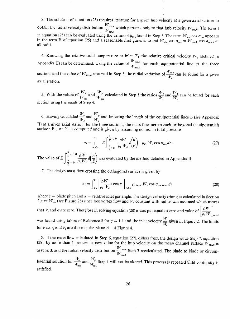
3. The solution of equation (25) requires iteration for a given hub velocity at a given axial station to Wins r
obtain the radial velocity distribution ~ which pertains only to that hub velocity Wms,h. The term 1
in equation (25) can be evaluated using the values of rims found in Step 3. The term Wms COS ams appears in the term II of equation (25) and a reasonable first guess is to put Wins COS ams = Wm~,h COS ams,h at all radii.
4. Knowing the relative total temperature at inlet T~ the relative critical velocity W~ (defined in WE$ r
Appendix II) can be determined. Using the values of ...... for each equipotential line at the three Wms,h
sections and the value of Wms,h assumed in Step 3, the radial variation o f ~ - ~ m~ can be found for a given ' ' c
axial station.
W s Wp . W, Wp 5. With the values o f - - and - - calculated in Step 1 the ratios - - and - - can be found for each
Wms Wms W c W c
section using the result of Step 4.
W s Wp 6. Having calculated ~ and ~ and knowing the length of the equipotential lines E (see Appendix
II) at a given axial station, for the three sections, the mass flow across each orthogonal (equipotential) surface, Figure 20, is computed and is given by, assuming no loss in total pressure
I/ r,0 ew_d(._)
,h .'~-=o ptW~ \EJ Ptl W~coSamsdr. (27) E
Z h e v a l u e o f E I ~ = I'0 pW ~/n~ - - - a ~ - ~ was evaluated by the method detailed in Appendix II.
= 0 p, \El
7. The design mass flow crossing the orthogonal surface is given by
m = s c o s ~ Pt inlet Wc c o s O'ms inlet dr (28) rh inlet
where s = blade pitch and ~ = relative inlet gas angle. The design velocity triangles calculated in Section 2 give Wci, (see Figure 26) since free vortex flow and Va constant with radius was assumed which means
that V~ and cr are zero. Therefore in solving equation (28)a was put equal to zero and value oflt_~,-c~P°~Wv¢-w]inlet
W was found using tables of Reference 8 for 7 -- 1.4 and the inlet velocity ~ given in Figure 2. The limits
for r i.e. r t and rh are those in the plane A - A Figure 4.
8. If the mass flow calculated in Step 6, equation (27), differs from the design value Step 7, equation (28), by more than 1 per cent a new value for the hub velocity on the mean channel surface Wms,h is
Wills r assumed, and the radial velocity distribution ~ Step 3 recalculated. The blade to blade or circum-
ferential solution for W~ Wp and - - Step 1 will not be altered. This process is repeated ~ntil continuity is Wms Wins
satisfied.
26
APPENDIX VI
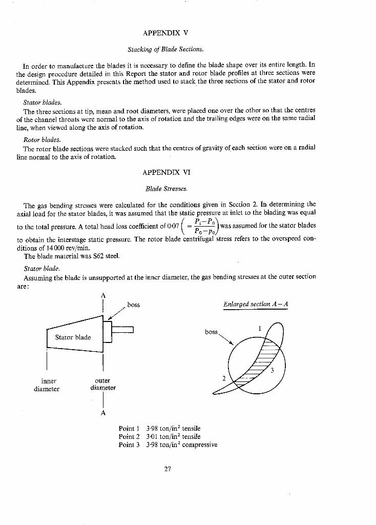
Stackin9 of Blade Sections.
In order to manufacture the blades it is necessary to define the blade shape over its entire length. In the design procedure detailed in this Report the stator and rotor blade profiles at three sections were determined. This Appendix presents the method used to stack the three sections of the stator and rotor
blades.
Stator blades. The three sections at tip, mean and root diameters, were placed one over the other so that the centres
of the channel throats were normal to the axis of rotation and the trailing edges were on the same radial line, when viewed along the axis of rotation.
Rotor blades. The rotor blade sections were stacked such that the centres of gravity of each section were on a radial
line normal to the axis of rotation.
Blade Stresses.
are :
The gas bending stresses were calculated for the conditions given in Section 2. In determining the axial load for the stator blades, it was assumed that the static pressure at inlet to the blading was equal
P~-Po'~ to the total pressure. A total head loss coefficient of 0.07 = ~ ) was assumed for the stator blades
to obtain the interstage static pressure. The rotor blade centrifugal stress refers to the overspeed con- ditions of 14 000 rev/min.
The blade material was $62 steel.
Stator blade. Assuming the blade is unsupported at the inner diameter, the gas bending stresses at the outer section
bo
A
boss /
inner outer diameter diameter
I A
Enlarged section A - A
APPENDIX V
Point 1 Point 2 Point 3
3"98 ton/in 2 tensile 3,01 ton/in 2 tensile 3"98 ton/in 2 compressive
27
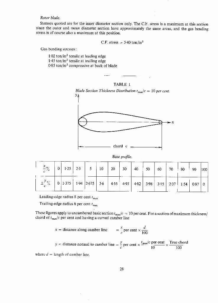
Rotor blade.
Stresses quoted are for the inner diameter section only. The C.F. stress is a max imum at this section since the outer and mean diameter section have approximately the same areas, and the gas bending stress is of course also a max imum at this position.
C.F. stress = 5.40 ton/in 2
Gas bending stresses:
1.02 ton/in 2 tensile at leading edge 1.45 ton/in 2 tensile at trailing edge 0.85 ton/in z compressive at back of blade
T A B L E 1
Blade Section Thickness Distribution tmax/C = 10 per cent.
chord c ~.~
Base profile.
x ~ 0 1-25 2"5 5 10 20 30 40 50 60 70 80
+=Uo 0 1"375 1-94 2'675 3"6 4'55 4"95 4"82 3-98 3"15 2"37 1"54 - - C
90
0'97
100
Leading-edge radius 8 per cent tma x
Trailing-edge radius 6 per cent tin, x
These figures apply to uncambered basic section tmax/C = 10 per cent. For a section of max imum thickness/ chord of tma,jC per cent and having a curved camber line
x d x = distance along camber line = - per cent x - -
c 100
y = distance normal to camber line = -Y- per cent x c
tmax/C per cent True chord x
10 100
where d = length of camber line.
28
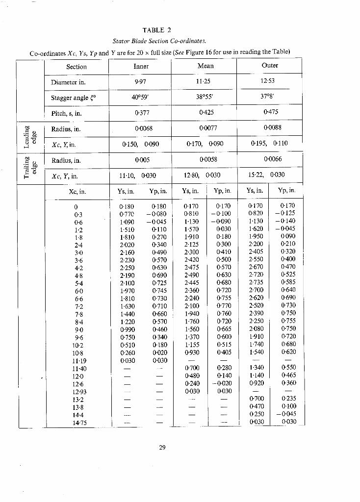
TABLE 2
Stator Blade Section Co-ordinates.
Co-ordinates Xc, Ys, Yp and Y are for 20 x full size (See Figure 16 for use in reading the Table)
CD ~D
Section
Diameter in.
Stagger angle ~o
Pitch, s, in.
Radius, in.
Inner Mean
9.97 11.25
40059 ' 38055 '
Outer
12.53
3708 '
0.377 0.425 0.475
0.0068 0.0077 0.0088
0-150, 0.090 0.170, 0.090 0.195, 0.110 Xc, Y, in.
~0 Radius, in. 0.005 0.0058 0.0066 . ~ t~
Xc, Y, in. 11.10, 0.030 12.80, 0-030 15.22, 0-030
Xc, in. Ys, in. Yp, in. Ys, in. Yp, in. Ys, in. Yp, in.
0 0.3 0.6 1.2 1.8 2.4 3.0 3.6 4.2 4.8 5-4 6.0 6.6 7.2 7.8 8.4 9.0 9.6
10.2 10.8 11.19 1 1 - 4 0
12.0 12.6 12.93 13.2 13.8 14.4 14.75
0"180 0'180 0"770 - 0"080 1"090 - 0"045 1"510 0"110 1"810 0'270 2"020 0'340 2"160 0"490 2"230 0'570 2"250 0"630 2"190 0"690 2"100 0"725 1"970 0"745 1"810 0"730 1"630 0"710 1"440 0'660 1"220 0"570 0"990 0"460 0"750 0"340 0.510 0.180 0.260 0.020 0.030 0.030
0.170 1 o.81o
1.130 1;570 1"910 2"125 2"300 2"420 2"475 2"490 2"445 2"360 2"240 2"100 1"940 1"760 1"560 1"370 1"155 0'930
0.700 0.480 0.240 0.030
0.170 -0 .100 -0 .090
0.030 0.180 0.300 0.410 0.500 0-570 0-630 0.680 0.720 0.755 0.770 0.760 0.720 0.665 0.600 0.515 0-405
0.280 0.140
- 0.020 0.030
0.170 0.820 1.130 1.620 1-950 2-200 2.405 2.550 2.670 2.720 2.735 2.700 2.620 2.520 2.390 2-250 2.080 1.910 1.740 1.540
1.340 1.140 0.920
0-700 0.470 0.250 0.030
0.170 -0 .125 -0 .140 - 0.045
0.090 0.210 0.320 0.400 0.470 0-525 0.585 0.640 0.690 0.730 0.750 0.755 0.750 0.720 0.680 0-620
0.550 0.465 0.360
0.235 0.100
- 0.045 0.030
29
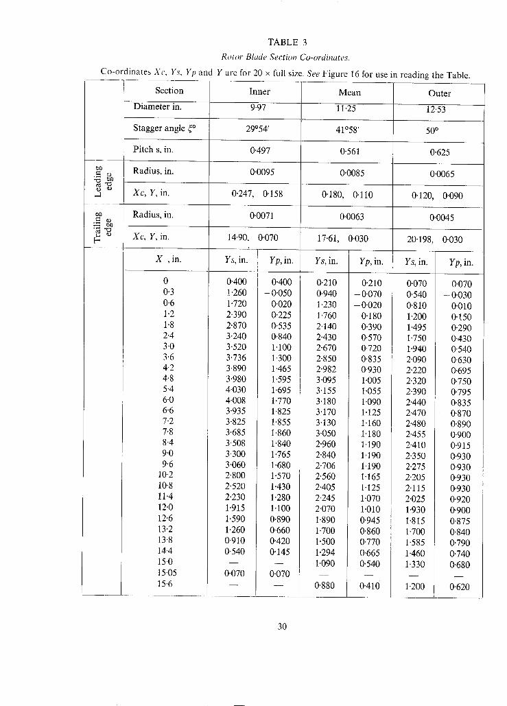
TABLE 3
Rotor Blade Section Co-ordinates.
Co-ordinates Xc, Ys, Yp and Y are for 20 × full size. See Figure 16 for use in reading the Table.
~0
.2
[-
Section
Diameter in.
Stagger angle ~o
Pitch s, in.
Inner
9'97
29°54 '
0.497
Mean
11"25
41058 '
0.561
Outer
12.53
50 °
0.625
Radius, in. 0.0095 0.0085 0.0065
Xc, Y, in. 0.247, 0'158 0'180, 0.110 0.120, 0.090
Radius, in. 0.0071 0.0063 0.0045
Xc, Y, in. 17.61, 0.030 20.198, 0-030 14-90, 0.070 /
Ys, in. Yp, in. Ys, in. Yp, in. X ,in. Ys, in.
0 0.3 0.6 1.2 1.8 2.4 3.0 3.6 4.2 4.8 5.4 6-0 6.6 7.2 7.8 8.4 9.0 9.6
10.2 10.8 11.4 12.0 12.6 13.2 13.8 14.4 15.0 15.05 15.6
0.400 !.260 1.720 2-390 2.870 3.240
3.520 3.736 3.890 3.980 4.030 4.008 3.935 3.825 3.685 3.508 3.300 3.060 2.800 2.520 2-230 1.915 1.590 1.260 0.910 0.540
0.070
0-400 -0"050
0.020 0.225 0'535 0.840 1.100 1.300 1.465 1-595 1.695 1.770 1.825 1.855 1.860 1.840 1.765 1.680 1.570 1.430 1.280 1.100 0.890 0.660 0.420 0"145
0.070
0.210 0.940 1.230 1.760 2.140 2-430 2.670 2.850 2.982 3.095 3.155 3.180 3.170 3-130 3-050 2.960 2.840 2.706 2.560 2.405 2.245 2.070 1-890 1.700 1.500 1.294 1.090
0.880
0.210 - 0.070 - 0.020
0.180 0.390 0.570 0.720 0.835 0.930 1-005 1-055 1.090 1.125 1.160 1.180 1.190 1.190 1.190 1-165 1.125 1.070 1.010 0.945 0.860 0.770 0.665 0.540
0.410
0.070 0'540 0.810 1 "200 1.495 1.750 1.940 2.090 2.220 2.320 2.390 2.440 2.470 2.480 2.455 2.410 2.350 2.275 2.205 2.115 2.025 1.930 1.815 1.700 1.585 1.460 1.330
1.200
Yp~ in .
0-070 -0 .030
0.010 0.150 0.290 0.430 0"540 0.630 0.695 0.750 0.795 0.835 0.870 0.890 0.900 0.915 0-930 0-930 0.930 0.930 0.920 0.900 0.875 0.840 0.790 0-740 0.680
0.620
30

TABLE 3--contd.
Section Inner Mean Outer
Xc, in. YS, in. Yp, in. Ys, in. Yp, in.
16.2 16.8 17.4 17.72 18.0 18.6 19.2 19.8 20.29
Ys, in. Yp, in.
0.670 0.270 0.460 0.120 0-240 - 0.040 0.030 0.030
1.065 0-932 0.805
0.648 0.520 0.372 0.226 0.030
0.540 0.475 0.390
0.299 0.220 0.115
- 0-023 0-030
TABLE 4
Final Blade Design Parameters.
Stator blade Rotor blade
Section diameter Inner Mean Outer Inner Mean Outer
Number of blades
Pitch/axial chords, s/%
Suction surface Diffusion parameter - D~ (Loss after trailing edge see Section 4.2.2)
Pitch/blade back curvature s/e
Zweifel loading coefficient
Or
Distance of point of maximum camber from leading edge, a/c per cent
Design incidence, degrees
0.898
0.117
0.264
0.25
83
0.850
0"071
0-212
0-760
40
0.810
0.142
0.171
0
0"766
0-158
0"308
0.892
40
0"50
63
0"853
0'133
0"173
0"769
37
0.962
0"185
0"117
0"678
37
0"10
31

o _J
t.d r~
(o) ZERO SWIRL
f 80 'to
86
8O
"~ e.q
Q- E
(D Z
O
LI
8~
F I G 1.
i f f f
( b ) OPI ' |~UM ~W|RL /" f ' '~m' .,,.~. OUTL~.T / I J SWIRL
/ ~ / . / ANGLE
- _ 91
0"5 I ' 0 1"5
FLOW COEFFICIENT Vo.l Um
3B
S6
Design point efficiency contours for a series of single stage turbines.
32
90"1.
~o
PLANE C- C 1~), = o . , - ¢ (~Y) = 0.255 c l
l V - (~c/ i -O" 281
STATOR
/ -_ I(~,¢) . o.,i~
( a ) o : ° " "
ROTOR BLADE
DIRECTION
OF ROTATION
PLANE B-D
. , / l !
(~olo = o . , . 0
0(2" -57" 4° ~ "O
.o,__~ C,,) i =C,, )o (we), = (wo),
~ 3 = tOO ,.~ e o..... (~3 : 9*
( ~ o / , - o . , , ~ / - ~ : " (-'vole: o . , , - - , -~ - , I N.G.T.E. SIGN CONVENTION REFERENCE I
I v ) = 0 . . , (~o/, : ° " °
INNER DIAMETER : 9 "97 in
(~o) :o. ,,,
MEAN DIAMEIER
: 11"25in
U _ (v~) , - o ~63
OOTER O,..E.ER = 12-53in
FIG. 2. Design velocity triangles.

4 ~
I - 6
/
CASCADE DATA
u.
0 . B u.
N
0 - 6
<
D - " - - "
O'- - - - -
[ ]
O
ROTOR
NOZZLE
ROTOR .~
STATOR
\ \
\
\ [] \
TURBINE TESTS I " ~ p']
MEAN DIAMETER
PRESENT DESIGN I
MEAN DIAMETER
I -50 -60 -70
GAS OUTLET ANGLE 0< 2
"I~T = 2 Cos 20~ 2 ( t a n O/~ I - t an ( X 2 ) S / C a
CK" 1 GAS INLET ANGLE l NG.T.E SIGN CONVENTION
OC 2 GAS OUTLET ANGLE . J REFERENCE !
STATOR
BLADE
8
A
ROTOR
BLADE
, ~ . ~ O" 1 ? 8 IN AT MEAN DIAMETER
A --it m
ua
c~
== .=
REFERENCE PLANES FOR VELOCITY TRIANGLES
INLET TO STATOR PLANE C-C
OUTLET FROM STATOR PLANE A - A
iNLET TO ROTOR PLANE A - A
OUTLET FROM ROTOR PLANE B-- B
AXIAL CHORDS ( INCHES)
DIAMETER
OUTER
MEAN
ROOT
IN IT IAL DESIGN
SEE SECTION 3'2
STATOR ROTOR
O, 565 O "$/,,4
O" 500 O" 593
0" ~22 O" 653
FINAL DESIGN
STATOR RO'rOR
0 - 585 0 • 653
O " 500 O" 658
O" 422 0. 650
FIG. 3. Blade loading correlation. FIG. 4. Contours of inner and outer walls.
L I N E A R V A R I A T I O N OF MASS FLOW PER UNIT t~ o u RADIUS OF A N N U L U S WITH A X I A L DISTANCE
' ~ ~ .1~ . -
• , , ,
A X I A L DISTANCE
u
I I
~ J
.,< i ,,< n.,, l -CO " I l
2 < Z 2: <( <( .~ <(
( j / -.,~ "ira i <[ I I
< <
u J . 7 ~ ~
i . 0,,-
o l i - - ~
7 _ 1 ~ ,..1
-! I I J I i I I
I j -
I I I I I I
I
A X I A L D I S T A N C E
cO
I I I
I i I
I I I
i I i I
2 o t I - ~ I I
"' ~ J L ~ , - o / ~ 1 I
I I I I I I f I i i
• ,, I I
i - /
t /
I , '~ '~_ ~ I u = . r ~ l ::)I>
I
I ~ >l:~ I
O
II II O
c~
uJi 4;:)1
35

0",
u 0 o
i °
I ' 0
DESIGN
INLET VELOCITY
0 " 2
J f
j "
SUCTION SURFACE
J / PRESSURE
~ R F A C E
0 "2 0"4 0 6
AXIAL DISTANCE X AXIAL CHORD o
PARABOLIC CAMBER LINE WITH POSITION OF MAXIMUM CAMBER AT /,O+/. OF CHORD S / C a : O 'BgS $/e : 0"26¢
~ D E S I G N OUTLET
VELOCITY ('AFTER LOSS) /
0 ' S I ' 0
FIG. 6. Design stator blade inner section dia. =
9-97 in. Two dimensional velocity distribution.
>,~
~ m
I ' 0
0 . 4
DESIGN INLET VELOCITY
0 ' 2
SUCTION S U R F ~
f f
PRESSURE ~ A C E
0-2 0"¢ 0 6
AXIAL DISTANCE X AXIAL CHORD Ca
0 " 8
PARABOLIC CAMBER LINE WITH POSITION OF
MAXIMUM CAMBER AT &O '/, CHORD S/Ca : O'$E0 SJe : O'21Z
FIG. 7. Design stator blade mean section dia. = 11.25 in. Two dimensional velocity distribution.
DESIGN OUTLET
VELOCITY (AFTER LOSS)
>1~. 0"
0 " 6
w
o
0 . 4
DESIGN
INLET VELOCITY
0 " 1
SUCTION J SURFACE
/ /
J
j Y PRESSURE
~ I R F A C E
0"2 O'.L 0 '6 0 - 15
AXIAL DISTANCE X
AXIAL CHORD ~0+
PARABOLIC CAMBER LINE WITH POSITION OF MAXIMUM CAMBER AT 40 +I+ OF CHORO
S : 0 '110 '~ : O,171
Ca
FIG. 8. Design stator blade outer section dia. = 12.53 in. Two dimensional velocity distribution.
IESIGN OUTLET
VELOCITY AFTER LOSS)
1 ' 0
°i ~- o - s
C~ vlV~
0"
0ESIGN INLE;
VELOCITY
0 ' 2 J
0"2 0 -
SUCTION SURFACE
J ~ S U R E
SURFACE
f
0 ' 6 0 " 8 I ' 0
AXIAL DISTANCE X_X AXIAL CHORD Ca
pARABOLIC CAMBER LINE WITH POSITION OF
MAXIMUM CAMBER AT t,0"h CHORD
S /Ca = 0 "766 SIl~ : 0 ' 308
FIG. 9. Design rotor blade inner section dia. = 9.97 in. Two dimensional velocity distribution.
DESIGN OUTLET
VELOCITY
(AFTER LOSS)
I - 2
CHOKED
L,O
DO
t
Ii u
• ~ : o .
DESIGN O" INLET VELOCITY
0.2
/ /
/ /
/ ~ ~ SUCTION ~ - - ~ ' ~ ' ~ ~URFAC E
/
" - #
/ /
0"2 0"4 0"
CHO.D
0"~, I ' O
AXIAL DISTANCE AXIAL CHORD o
PLO $1Ca : 0 "90C s l e : 0 "308( IN IT IAL DESIGN)
P60 S/Ca : 0 "871 SI~ : 0 ' 2 7 3
P30 SICa : O' 886 SIE : 0 "025
DESIGN OUTLET
VELOCITY (AFTER LOSS)
PARABOLIC CAMBER LINE WITH POSITION OF MAXIMUM CAMBER AT 60 *1. AND 30 "1. OF CHORD
FIG. 10. Rotor blade mean section diameter = 11-25 in. T w o dimensional velocity distr ibut ion--I .
~:1~" , . o
?-
ua >
0
o
0
DESIGN 0 -
INLET VELOCITY
0 " 2
r SUCTION
SURFACE ~
!
0"2 0"L 0 " 6 0"S ! " 0
AXIAL DISTANCE X. AXIAL CHORD Co
f i I . I I . "
/ / e . / / i /
P~O S/Co : 0"SS& $1e : 0"3OS
P37 S / C o : 0"999 Sle : 0 "227
. . . . . P37 $1Co : 0"853 SIC : 0 " [ 7 3 (FINAL OESION)
PARABOLIC CAMBER LINE WITH POSITION OF MAXIMUM CAMBER AT 37"1. AND 4D'I. OF CHORD
FIG. 11. Rotor blade mean section diameter = 11.25 in. T w o dimensional velocity d is tr ibut ion--II .
DESIGN OUTLET
VELOCITY (AFTER LOSS)

~ u
o.~, 0
O , I ,
DESIGN INLET VELOCITY
0 " l
,~UCTION SURFACE
/ / /
/ /
, / /
/," /
/ / / / /
" / ~ PRESSURE SURFACE
/
0 . 4 0 " 6 O 6 1 . 0
AXIAL DISTANCE X~ AXIAL CHORD Ca
DESIGN OUTLET
VELOCITY (AFTER LOSS)
~-- 0
~ u
~ u O
O , g
OESIGN
INLET VELOCITY
0 . 1
SUCTION SURFACE
s / / , / / / ~ //1I~ SURE
SURFACE / /
/
/ / /
0 ' 2 O . 6 0 'S 0.11
AXIAL DISTANCE X AXIAL CHORD '~a
IESIGN OUTLET
(AFTER LOSS)
I -O
P/-.O. S/Ca :, 1"231p S/e : O-2BO (INITIAL DESIGN)
P37~ S/Ca : 1"180~ SIe : 0"17/,
. . . . . P37, S/Ca : 0"856~ SIC : 0"075
PARABOLIC CAMBER LINE WITH POSITION OF MAXIMUM CAMBER AT 37"1. AND 1,0"l, OF CHORD
FIG. 12. Rotor blade outer section diameter = 12.53 in. Two dimensional velocity distribution--I.
P]I?, S/Ca : 0"952j S/~ : 0"117 (FINAL DESIGN)
P37 a SICa : 0"SSE, S IC ; 0 ' 0 7 5
PARABOLIC CAMBER LINE WITH POSITION OF MAXIMUM CAMBER AT ] 7 t l , OF CHORD
FIG. 13. Rotor blade outer section diameter = 12-53 in. T w o dimensional velocity distribution--II.
OUTER SECTION
OIAMET
C~
O N
OUTER SECTION
° - - .
MEAN SECTION
DIAMETER 11 = . .
0 0-1 0-2 0-3 0 '4 0'S IN,
DIAMETER : g ' 9 .
! J. [ 1 I I 0 0'1 0-2 0,3 0"4 0-5
IN ,
FIG. 14. Profile of stator blade at inner mean and outer diameters (see Fig. 4 for location of sections).
FIG. 15. Profile of rotor blade at inner mean and outer diameters (see Fig. 4 for location of sections).
l! i __ U I I I I SECTION
. . . . . . . . . SECTION
ROTOR BLADE
INNER SECTION
SEE TABLES 'IT AND "n'T
AXIS OF ROTATION
(a) SIDE VIEW OF STATOR AND ROTOR BLADES
Y POSITIV E
STAGGER ~ + VE AS DRAWN
XlS OF ROTATION STA~OR O L A D R ~
POSITIVE
(b) TOP VIEW OF STATOR AND ROTOR BLADES
FIG. 16. Side and top view of stator and rotor blades for use with Tables 2 and 3.
1 , 0
o ~ O.B ~ > > ~ ~ o ~E o ~
~ w
W w
DESIGN INLET
VELOCITY 0"4
0.2
I SUCTION SURFACE
/ I
THROAT
/S SURFACE
~ ~ ' ~ ~ ~ " ~ DESIGN OUTLET
j / / / / ( A F TER LOSS)
, / / .
0-2 0"4 0'6 O'S l'O
AXlAt DISTARCE X AXIAL CHORD C a
20 SOLUTION MASS FLOW PER UNIT RADIUS OF ANNULUS VARIES LINEARLY FROM LEADING TO TRAILING EDGES OF BLADE
3 D ZERO CURVATURE I
m
m
&
RADIAL FLOW ANGLE ~1 VARIES LINEARLY FROM ROOT TO TIP
RADIAL FLOW ANGLE ~ = G" = 0
RADIAL FLOW ANGLE VARIES LINEARLY FROM ROOT TO TIP
I FLARE STARTS AT p, LEADING EDGE OF
ROTOR BLADES
FLARE STARTS MID-WAY BETWEEN STATDR AND ROTOR BLADES
(PLANE A°A FIEi. /g)
FIG. 17. Design rotor blade inner section dia. = 9.97 in. Comparison of two-dimensional and three-
dimensional velocity distribution.
t ~
o~ ~- 0"81
0"6
DESIGN 0"4 INLET VELOCITY
0 .2
I SUCTION SURFACE
/ /
/
I THROAT
. " PR SSURE SURFACE
0"2 0.4 0-6
AXIAL OISTANCE X
AXIAL CHORD C a
0-8, I ,O
2D SOLUTION MASS FLOW PER UNIT
RADIUS OF ANNULUS VARIES LINEARLY FROM LEADING TO TRAILING EDGES OF BLADE
DES#GN OUTLET
VELOCITY (AFTER LOSS)
I ,O
_ o u o 0"8
u ~
uJ ~ 0"6
0'4
DESIGN
INLET VELOCITY
0"2
THROAT
0 0"2
I SUCTION SURFACE
/ /
/ /
/ /
,.. " ->~ j
/ -
/ . " / f . , "
/ /
~ C E t / ' ' " pRESSURE
0-4 0"6 AXIAL DISTANCE X AXIAL CHORD CO
0 8 I ' D
DESIGN OUTLET
VELOCITY
(AFTER LOSS)
f 2D SOLUTION MASS
FLOW PER UNIT RADIUS ANNULUS VARIES LINEARLY
. . . . FROM LEADING TO TRAILING EDGES OF BLADE
FROM PLANE MID-WAY BETWEEN STATOR AND
ROTOR BLAOES (PLANE A - A FIG 4) TO TRAILING EDGE
3D ZERO CURVATURE SOLUTION
RADIAL FLOW ANGLE VARIES LINEARLY FROM
ROOT TO TIP
RADIAL FLOW ANGLE
~ = O ' = O
RADIA[ FLOW ANGLE VARIES LINEARLY FROM ROOT TO TIP
t FLARE STARTS AT LEADING EDGE OF ROTOR BLADES
FLARE STARTS MIDWAY BETWEEN STATOR AND ROTOR BLADES (PLANE A -A FIG+ ,tt )
3D ZERO CURVATURE
SOLUTION E~
A
RADIAL FLOW ANGLE ~ " ~
VARIES LINEARLY FROM I FLARE STARTS AT ROOT TO TiP LEADING EDGE OF
ROTOR BLADES
RAD#AL FLOW ANGLE
~" =O" = 0
RADIAL FLOW ANGLE * ~ FLARE STARTS MID WAy
VARIES LINEARLY ~J~ BETWEEN 5TATOR AND ROTOR FROM ROOT TO TIP BLAOES (PLANE A - A F IG4 )
FIG. 18. Design rotor blade mean section dia. = 11-25 in. Comparison of two-dimensional and three-
dimensional velocity distribution.
FIG. 19. Design rotor blade outer section dia. = 12-53 in. Comparison of two-dimensional and three-
dimensional velocity distribution.

ACCELERATION RADIAL VELOCITY j l ' ~ - - ~ MERIOIONAL
PARTICLE OF FLUID._.._. FORCE ~ D~ ~ VELOCITY Wm
L ~ ~ I Jl~ AXIAL VELOCITY Vel
MERIOIONA k ~TREA.L,NE / I
CF.tJTRIFUGAL FORCE pVw 21 g~ !
AXIS OF ROTATION I
(a )FORCES ACTING IN RADIAL DIRECTION
SELECTE0 AXIAL STATION l FOR RADIAL EQUILIBRIUM I /
PRESSURE SUCTION SURFAC£
SURFACE
ORTHOOONAL •P (~gUIPOTENTtAL)~ Va SURFACE
TIP We!
g
AN CHANNEL SURFACE
ROOT - -
J~ AXIS OF ROTATION J
(b) MEAN CHANNEL SURFACE
FIG. 20. Force diagram and mean channel surface for radial solution.
,<
m
i
. OUTER SE
R O T O R ~ ~
I
CTION HAMETER 12"53 IN-
MEAN SECTION DIAMETER 11.25 iN.
iNNER SECTION DIAMETER 9 97iN
DESIGN VELOCITY TRIANOLES ,~QINLET PLANE A.A ASSUMED TO OCCUR AT OUTLET PLANE B-B THROAT
CENTRE LINE B
X DESIGN VELOCITY TRIANGLES "~ CALCULATED FROM
30 ZERO CURVATURE SOLUTION J CONTINUITY . . . . . 2D SOLUTION - MASS FLOW AS IN FIG, S
FI~.21. Streamline geometry calculated from three-dimensional zero curvature solution.
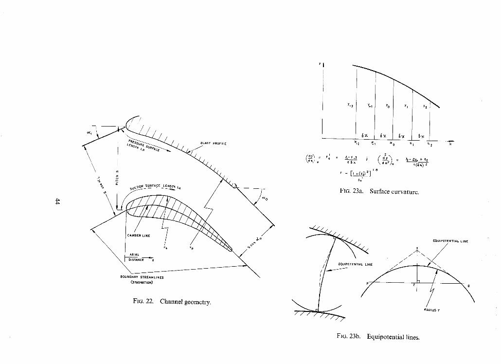
4~
O< i
/
, / / ,
\ 4=
\ SURFACE
TANCE X
80UNDARY STREAMLINES CSTAGN&TION)
FIG. 22.
BLADE PROFILE
L=
rp
Channe l geometry .
9 j_o
Y-2 Y-1 YO I Y! Y2
I
6x, ~;~c J -2 ~I
('a_y'~ ~ Yo Yl-Y- | j ( d 2 Y 2 ) = y2 - 2ye .1. y_2 \,~x/o 2 s----~ ~ o " 4(~.) 2
= [, ,(,o'~ =] " ~
Yo"
FIG. 23a. Surface curvature.
EQUIPOTENTJAL LINE
I I - - 7 / / EOUIPO r ENTIAt lINE . / • / ~
FIG. 23b. Equipotent ia l lines.
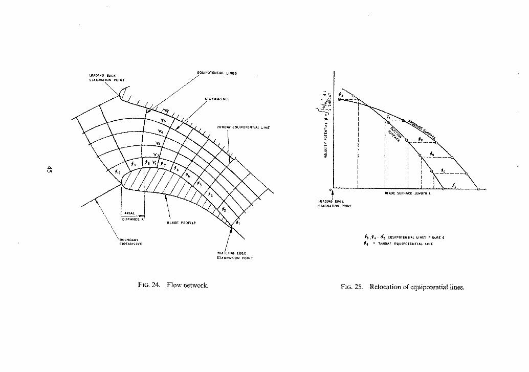
EQUIPO*I'ENTIAL LINES
TRAiLiNG EDGE STAGNATION POINT
o
~ 8 m
l i ~ \ , \
! c ! IN \ t I i t , , , \
OI BLADE SURFACe[ LENGTH L
LEADING EDGE STAGNATION POINT
~[3 ~4"" '~8 EOUIPGTEHTIAL LINES FIGURE 6
J~3 = THROAT E~U~0TENTIAL LINE
FIG. 24. F l o w network. FIG. 25. Re loca t ion o f equipotent ia l lines.

V I-
-----e~ V Q
\ \
~ . -Z
Vr
Vw Vr
Vc
Va
W Vr
o-
,~m=-
Wci
FIG. 26.
~ AXIS OF ROTATION
SIGN CONVENTION
,><, IB N.G.T.E. (REF. I.)
~{, 0" "F VE AS DRAWN
Co-ordinate system and velocity components.
46
Part II--Test Performance of Design Configuration
By D. J. L. Smi th and D. J. F u l l b r o o k
Summary. To check theoretical prediction methods the turbine stage described in Part I of this Report has been
tested extensively on a cold flow experimental rig over a wide range of operating conditions. The test results have been compared with performance figures calculated by the method currently in use at the National Gas Turbine Establishment.
The predictions are in good agreement with observed efficiencies and swallowing capacities. At design flow conditions the test total-total isentropic efficiency is 92.2__ 0.5 per cent. This compares with a pre- dicted value of 92.5 per cent.
The flow conditions at the turbine exit were estimated by through-flow analysis and compared with experimental observations. Ignoring end wall boundary-layer effects the advanced theory gives a good estimate of the exit axial velocity profile.
CONTENTS
1. Introduction
2. Description of Experimental Rig
2.1. The turbine
2.2. The test facility
2.3, Instrumentation
2.3.1. Air mass flow
2.3.2. Power
2.3.3. Turbine air pressures
2.3.4. Turbine air temperatures
2.3.5. Turbine speed and rotor tip clearance
2.3.6. Traverse gear
3, Turbine Performance
3.1. Calculated Performance
3.2. Test Performance
4. Traverse Results
4.1. Axial Velocity and Gas Angle 4.2. Deduced Outlet Gas Angles from Rotor Blades
4.3. Radial Variation of Blading Efficiency
47
5. Conclusions
5.1. General
5.2. Analytical
List of Symbols
References
Appendix--Turbine flowmeter calibration
Tables ! and 2
Illustrations--Figs. 1 to 20
Detachable Abstract Cards
No,
1
2
Traverse results
Inlet flow conditions
LIST OF TABLES
Title
Fig. No.
1
2
3
4
5
6
7
8
9
10
11
12
13
14
15
LIST OF ILLUSTRATIONS
Title
Turbine annulus
Test facility
Turbine inlet conditions
Arrangement of turbine annulus and instrumentation
Estimated gas angles and loss coefficients
Rotor tip clearance
Stage efficiency - design speed, N/w/--~ = 685
Swallowing capacity and stage loading--design speed, N/~/-~ = 685
Stage efficiency - ~ design speed, N/~-~ = 600
Swallowing capacity and stage loading ~ design speed, N/~/-~ = 600
Stage efficiency--~] design speed, N/~/~ = 514
Swallowing capacity and stage loading--~ design speed, N/n/~ = 514
Stage efficiency--~ design speed, N/w/-~i = 428
Swallowing capacity and stage loading---~ design speed, N/w/-~ = 428
Exit swirl angle
48

16 Static pressure and swirl angle at turbine exit (plane C Figure 4)
17 Exit flow conditions--design point
18 Comparison of predicted and measured axial velocity and swirl angle at turbine exit--design point (plane C Figure 4)
19 Mean relative flow angles at exit from the rotor row
20 Radial variation of blading efficiency
1. Introduction. The task of t he~turbine designer is necessarily that of achieving a satisfactory compromise between
the rival claims" of efficiency, size, weight, mechanical integrity (which may demand blade cooling) and other factors such as cost. In many instances he is constrained from simply designing a turbine which, solely from considerations of aerodynamic loading, has the highest possible efficiency. As a result the blading has usually been more highly loaded than consideration of efficiency alone would dictate and little is known about the conditions under which optimum efficiency is obtained.
The single-stage experimental turbine was designed as a test vehicle in which all the leading parameters (stage loading, flow coefficient, pitch/chord ratio, blade profile shape and aspect ratio) were selected conservatively to accord with current ideas for ensuring a reasonably high level of aerodynamic efficiency.
The blade profiles were laid out in a systematic manner from a symmetrical aerofoil profile shape set around a parabolic camber line. The blade spacing was selected using the criterion that the adverse pressure gradients on the suction surface should be on or near to the limit to avoid local separation of the boundary layer. A detailed description of the aerodynamic design procedure is recorded in Part I of this Report.
This Report describes a series of tests on this blading to determine the overall performance characteris- tics. Comparisons are made with theoretical estimates of turbine performance based on the standard 1 method currently in use at the National Gas Turbine Establishment. The flow conditions at the turbine exit are also estimated by the 'through-flow' analysis, reported in Reference 2, and compared with ex- mental observations.
2. Description of Experimental Rig.
2.1. The Turbine. The velocity diagram analysis and the method employed to design the blading for the subject turbine
are discussed in Part I of this Report which contains the dimensions of the turbine and tables of blade co-ordinates for both the stator and rotor rows.
Briefly, the turbine comprises a large inlet volute which leads into an initially parallel annulus of 13 in. outside diameter and 9.5 in. inside diameter, followed by a gentle contraction to a further parallel section containing the stator blades. The stator row of 83 blades has inner and outer diameters of 9.97 in. and 12.53 in. respectively. The annulus then diverges, as shown in Figure 1, to give an inner diameter of 9.5 in. and an outer diameter of 13 in. at outlet from the rotor row, which consists of 63 blades with plain radial tip clearances.
The rotor blades were mounted by a circumferential fir tree root between two disc halves having corresponding grooves cut in each rim. The complete disc was overhung and carried by a shaft running in ball and roller bearings. Following the rotor was a further length (6.2 in.--about four blade heights) of parallel annulus which carried the outlet instrumentation and thence led to the exhaust cone and the outlet ducting.
The blading was designed for free vortex flow and simple radial equilibrium, and at the mean diameter gave approximately 50 per cent reaction. The basic design parameters for the subject experimental
49
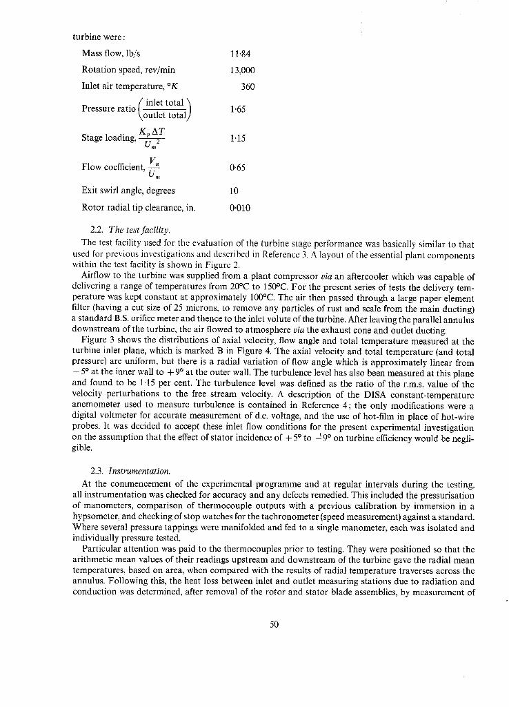
turbine were :
Mass flow, Ib/s 11-84
Rotation speed, rev/min 13,000
Inlet air temperature, °K 360
( .,et Pressure ratio \ou--~et t-otaiJ 1.65
Stage loading, Kv AT 1.15 Urn 2
Flow coefficient, V~ U---~ 0'65
Exit swirl angle, degrees 10
Rotor radial tip clearance, in. 0.010
2.2. The test facility.
The test facility used for the evaluation of the turbine stage performance was basically similar to that used for previous investigations and described in Reference 3. A. layout of the essential plant components within the test facility is shown in Figure 2.
Airflow to the turbine was supplied from a plant compressor via an aftercooler which was capable of delivering a range of temperatures from 20°C to 150°C. For the present series of tests the delivery tem- perature was kept constant at approximately 100°C. The air then passed through a large paper element filter (having a cut size of 25 microns, to remove any particles of rust and scale from the main ducting) a standard B.S. orifice meter and thence to the inlet volute of the turbine. After leaving the parallel annulus downstream of the turbine, the air flowed to atmosphere via the exhaust cone and outlet ducting.
Figure 3 shows the distributions of axial velocity, flow angle and total temperature measured at the turbine inlet plane, which is marked B in Figure 4. The axial velocity and total temperature (and total pressure) are uniform, but there is a radial variation of flow angle which is approximately linear from
- 5 ° at the inner wall to + 9 ° at the outer wall. The turbulence level has also been measured at this plane and found to be 1.15 per cent. The turbulence level was defined as the ratio of the r.m.s, value of the velocity perturbations to the free stream velocity. A. description of the DISA. constant-temperature anemometer used to measure turbulence is contained in Reference 4; the only modifications were a digital voltmeter for accurate measurement of d.c. voltage, and the use of hot-film in place of hot-wire probes. It was decided to accept these inlet flow conditions for the present experimental investigation on the assumption that the effect of stator incidence of + 5 ° to ~ 9 ° on turbine efficiency would be negli- gible.
2.3. Instrumentation.
At the commencement of the experimental programme and at regular intervals during the testing, all instrumentation was checked for accuracy and any defects remedied. This included the pressurisation of manometers, comparison of thermocouple outputs with a previous calibration by immersion in a hypsometer, and checking of stop watches for the tachronometer (speed measurement) against a standard. Where several pressure tappings were manifolded and fed to a single manometer, each was isolated and individually pressure tested.
Particular attention was paid to the thermocouples prior to testing. They were positioned so that the arithmetic mean values of their readings upstream and downstream of the turbine gave the radial mean temperatures, based on area, when compared with the results of radial temperature traverses across the annulus. Following this, the heat loss between inlet and outlet measuring stations due to radiation and conduction was determined, after removal of the rotor and stator blade assemblies, by measurement of
50
the temperature drop at a representative range of mass flows and inlet air temperatures. These values were later applied as small corrections, ranging from 0.2°C to 1.0°C, to the measured values of turbine temperature drop (see Section 3.2).
2.3.1. Air massflow. Air mass flow measurement was by standard B.S. orifice meter. The accuracy of this meter has been confirmed by flow tests using a calibrated nozzle. A summary of this work is con- tained in the Appendix.
2.3.2. Power. For power absorption the turbine was connected to a high speed water brake, the carcase of which was supported in oil-floated trunnion bearings. These provided an excellent mounting with negligible friction and the torque measurement was accomplished by a combination of accurate tare weights and a sensitive spring balance.
2.3.3. Turbine air pressures. The positions for the measurement of total and static pressures around the single-stage experimental turbine are illustrated in Figure 4.
(a) Turbine entry.
Inlet total pressure was measured by four single-point pitot tubes set at the mean diameter in plane A. In the same plane were four static pressure tappings on the outer wall. The local measured value of total pressure was modified by a calibration 5 derived from inlet traverses to give a true mean inlet pressure. The calibration can be expressed as an equation :
Pi = 0"943 Pins t . . . . . t + 0"057 Pi
In addition four static pressure tappings were provided in both the inner and outer walls, just upstream of the stator blades (plane B). These were necessary for determining the radial variation of axial velocity at the turbine inlet, discussed in Section 2.2.
(b) Turbine exit.
Ten static tappings in both the outer and inner waUs were located at approximately 2.70 in. downstream of the rotor blades in the parallel exit measuring section.
Tlae outlet total pressure was measured at plane D by five Kiel-type pitot rakes each with six pitot tubes. These were spaced radially such that each was positioned at the arithmetic mean diameter of an annular ring equal in area to one sixth of the total annulus area. A previous calibration showed them to be insensitive to variations of _ 30 ° in flow angle, measured froha the axial direction.
2.3.4. Turbine air temperatures. Four stagnation shielded thermocouples (connected in series) set in the inlet volute were used to measure the turbine inlet total temperature Ti. At the turbine exit the temperature was measured by eight thermocouples (also connected in series) positioned downstream of a honeycomb straightener and gauze.
The thermocouples were connected via an ice junction to a high grade potentiometer having a resolu- tion better than _+ 0.05°C.
2.3.5. Turbine speed and rotor tip clearance. The turbine rotational speed was measured by means of an impulse tachronometer and also by a Venner electronic counter. The former measured the period in which a set number of pulses occurred derived from a cam-operated microswitch geared to the turbine shaft. The latter was connected to one output phase of the shaft driven E.S.I. generator, and measured the time interval in which a set number of revolutions occurred. The two speed measurements were used as a cross check and both methods were in agreement.
The rotor tip clearance was measured with a Fenlow probe 6 mounted on the turbine casing in line with the plane of rotation.
2.3.6. Traverse 9ear. A small traverse gear carrying a claw-type pitot yawmeter and positioned in plane C approximately four blade chords downstream of the rotor blades was used to provide distribu- tions of total pressure and swirl angle at the turbine exit. The traverse data were used to provide the
51

flow angles necessary for the calculation of outlet total pressure from measured values of static pressure and air mass flow as detailed in Section 3.2. Also from the data the flow angles relative to the rotor blade and the axial velocities were calculated. By fitting appropriate probes the traverse gear was also used for the determination of outlet total temperature and static pressure distributions.
Immediately upstream of the stator blades, in plane B, provision was made for another traverse gear fitted with a pitot yawmeter or alternatively a thermocouple. This enabled the radial variations of inlet velocity, flow angle and total temperature to be determined ; these are discussed in Section 2.2. The traverse gear was replaced by an adapter supporting a hot-film probe when measuring the air stream turbulence.
3. Turbine Performance. f
3.1. Calculated Performance. One object of this experiment was to compare the measured performance with predictions based on
the method 1 currently employed at the National Gas Turbine Establishment. The calculation requires preliminary estimation of gas outlet angle and loss coefficient for each blade row and this information is shown in Figure 5*. The gas angles at mean diameter were calculated according to empirical rules for outlet Mach numbers of 0.5 and 1.0 and the assumption was made that the gas angle varied linearly between M = 0.5 and 1.0. The loss coefficients and gas angles were based on the design values of blade opening/pitch at the mean diameter and in the case of the rotor row, the design tip clearance. The in- spection figures for opening/pitch are compared with the design values in the Table below.
Stator Rotor
Design 0.520 0.491
Inspection 0.523 0.495
The design rotor tip clearance was 0-016 in. which is 0.69 per cent of the mean blade height. The tip clearances measured during the course of testing are shown graphically in Figure 6. It may be seen that the mean level of clearance is 0.007 in. which is 0.48 per cent of the blade height. To allow for the effects of radial tip clearance on isentropic efficiency the following empirical expression may be used:
where k tip clearance
h blade height
and X = 1.5 for rotor clearance only
= 3.0 for clearance on both stator and rotor.
From the above expression it may be seen that a change in k/h from 0.69 to 0.48 corresponds to an in- crease in efficiency of 0.32 per cent. Therefore, in comparing the test performance with predictions, this must be borne in mind.
The calculated values of efficiency and flow are shown superimposed on the general test results and are discussed with reference to the test results in the following Section.
52
3.2. T e s t Performance.
The test performance was measured at four values of non-dimensional speed and is presented in Figures 7 to 14 in the form of characteristics of blading efficiency versus stage loading, stage loading versus
pressure ratio and swallowing capacity versus pressure ratio. The exit swirl angles are plotted on Figure 15. Predicted values are also shown on each characteristic for comparison.
The efficiency is the usual 'isentropic' value, defined as the actual temperature drop AT, experienced by the gas in flowing through the stage, divided by the temperature drop ATise, corresponding to isen- tropic expansion from the measured inlet total temperature and pressure to the measured outlet total pressure. In each of the Figures 7, 9, 11 and 13, three different plots of test efficiency are shown. These efficiencies were based on differently derived values of AT and/or ATise; as detailed below:
(a) /'/bm- 'brake/measured efficiency' AT is the temperature drop equivalent of the work output, calculated from measurements of brake
torque, rotational speed and air mass flow. ATi~e is based on the measured inlet and outlet total pressures P~m and Pare respectively. (b) r/be- 'brake/continuity efficiency' AT is the same as for the brake/measured efficiency, (a). ATi~e is based on the measured inlet total pressure and on an outlet total pressure, Pa¢, calculated
from the average exit swirl angle, outlet static pressure and air mass flow. (C) /']em- 'couples/measured efficiency' AT is a corrected measured temperature drop obtained from inlet and outlet thermocouples with a
correction for heat loss by conduction and radiation as described in Section 2.3. ATi~ is the same as for (a). In calculating the outlet total pressure for ~/b~, the assumption was made that the outlet static pressure
varied linearly across the annulus from the measured value at the inner wall to that at the outer wall. Figure 16 shows static pressure and swirl angle traverses at design and seven eighths design speed; the average swirl values were 14 ° and 3 ° respectively. Both the hub and tip static pressures are seen to be in agreement with the traverse measurement and the traverses provide satisfactory confirmation of the assumed linear variation of static pressure.
The Reynolds number¢ of the flow through the stator varied from 2.15 × 10⁵ to 3.65 × 10⁵. For the rotor row the corresponding Reynolds number range was 2.5 × 10⁵ to 4.3 × l0 s.
It will be observed that most of the test points lie within a scatter band of +0.5 per cent in efficiency and that, in general, the current method of predicting turbine performance gives a good estimate of blading efficiency over a wide range of operating conditions. Taking the conservative value of efficiency (brake/continuity), then at design flow conditions the test efficiency is 92.2 per cent. This compares with an estimated value of 92.5 per cent.
The comparison of the efficiency characteristics based on brake readings and those based on the measured stage temperature drop provide a satisfactory check on the torque weighing system and on the mass flow measurement. At the design and seven eighths design speed there is little difference between the characteristics. For the lower speeds of three quarters and five eighths design speed there is a dis- crepancy of 1 per cent. At these speeds the correction for heat loss by radiation and conduction was a large percentage of the measured stage temperature drop and there was a scatter sufficient to bring the couples measured efficiencies in line with the brake measured values.
The results for swallowing capacity (mass flow) show even less scatter than the efficiencies. At the design speed the predictions indicate 1 per cent less flow up to a pressure ratio of 1.75 increasing to 2 per cent at choking conditions. For seven eighths design speed the agreement between prediction and test is extremely good and at the lower speeds the predictions are 1 per cent too high. The difference between test and calculated mass flows suggest a discrepancy between actual and estimated flow areas. From analysis of the traverses at the turbine exit, discussed in the following Section, it would appear that the major discrepancy lies in the stator flow area.
¢Reynolds number is based on blade chord, gas relative outlet velocity, outlet gas density and outlet gas viscosity.
53
4. Traverse Results.
4.1. Axial Velocity and Gas Angle.
During testing radial traverse measurements of total pressure and swirl angle were made at the turbine exit, plane C, Figure 4. Using these measurements, the flow angles relative to the rotor blade row, ~2 and axial velocity V a were calculated.
The design stage loading, Kp AT~Urn 2, and speed, N/x /~ , of the 'subject turbine are 1.15 and 685 respectively. The distributions of relative gas angle, axial velocity and swirl angle at the turbine exit for these conditions are shown in Figure 17. The inlet flow conditions were :
Mass flow 11.33 Ib/s
Inlet stagnation temperature 356°K
Inlet stagnation pressure 25.51 lb/in 2 abs.
From the plane of the rotor trailing edge to the traverse plane, there is an increase in flow area (Figure 4) of approximately 10 per cent. The gas angles shown for the rotor trailing-edge plane were calculated from the traverse data by applying conservation of angular momentum and continuity, assuming the radial distribution of mass flow to be unchanged between the two planes.
In the design of the blading the stagger angles were calculated so that the passage geometry at outlet satisfied the design flow angles using the method of Reference 1. This method can be termed a 'strip theory' in that it involves the calculation of the gas flow conditions at inlet and outlet from each blade row at a reference diameter which for this turbine is the mean diameter. To apply this method to the root and tip diameters the assumption was made that gas angle correction for the rotor blades, due to the finite radial tip clearance, varied linearly from root to tip being zero at the root diameter. Bearing this in mind, it will be observed that the test flow angles are in reasonable agreement with the design values. At the mean diameter the design flow angle is 59.75 ° . This compares with the momentum mean of the test values of 60.6°; there is a discrepancy of 0.85 °. Estimated flow angles with no allowance for tip clearance are also shown in Figure 17, and it may seem that if anything the measure of agreement with experiment is better, suggesting that the effect of tip clearance is in fact confined to the tip region. At mean diameter this estimated flow angle is 60.2 ° giving a discrepancy of only 0-45 °.
The internal aerodynamics of the turbine have been examined, for the above inlet flow conditions, by the 'through-flow' analysis reported in Reference 2. This advanced method of analysis determines the behaviour of the flow inside the blade rows along a mean stream surface. In between the blade rows and upstream and downstream of the machine, fluid particles are not confined to a mean stream surface but angular momentum is conserved.
The stream surface is prescribed in terms of two flow angles 2 and #. The angle 2 is the angle, in the plane containing the radial and circumferential velocity components at the mean stream surface, between the tangent to the surface and the radial direction. The angle/t is the angle, in the plane containing the axial and circumferential velocity components at the mean stream surface, between the tangent to the surface and the axial direction. The values of/t at inlet to and outlet from the blade row are known from the design velocity triangles. It was assumed that/~ varied linearly with axial distance from/~in~e, at the leading edge to ~outlet at the trailing edge.
The effects of irreversibility are introduced by defining a local polytropic efficiency for compression and expansion. In the present analysis the local polytropic efficiencies were assumed to be constant throughout the flow field and were chosen by trial and error until the analysis for the chosen mass flow and rotational speed gave an overall total pressure ratio which agreed with the observed value. This resulted in a local polytropic efficiency for compression and expansion of ~/pc = r ] p t = 0.93. The overall total-total isentropic efficiency given by the through-flow analysis was 92 per cent. This compares with the test values of 92.2 per cent, a discrepancy of 0.2 per cent. From Figure 18 it will be observed (noting the large scale) that, ignoring end wall boundary-layer effects the calculations done using the advanced through-flow theory gave a fair estimate of the axial velocity at the turbine exit. The agreement between
54
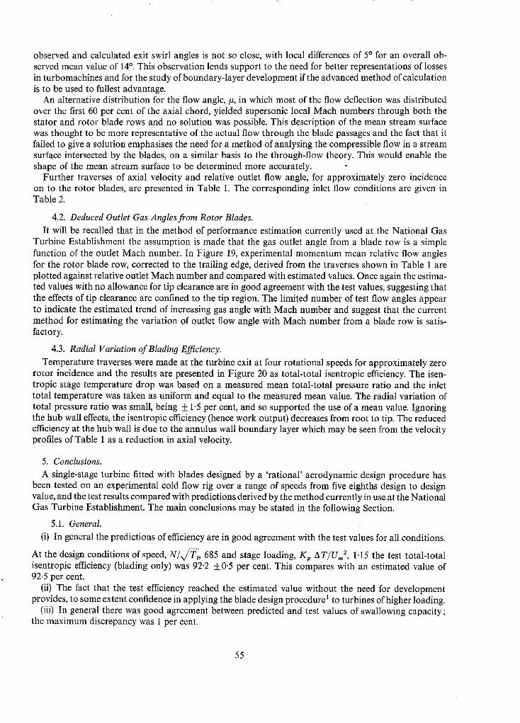
observed and calculated exit swirl angles is not so close, with local differences of 5 ° for an overall ob- served mean value of 14 ° . This observation lends support to the need for better representations of losses in turbomachines and for the study of boundary-layer development if the advanced method of calculation is to be used to fullest advantage.
An alternative distribution for the flow angle, #, in which most of the flow deflection was distributed over the first 60 per cent of the axial chord, yielded supersonic local Mach numbers through both the stator and rotor blade rows and no solution was possible. This description of the mean stream surface was thought to be more representative of the actual flow through the blade passages and the fact that it failed to give a solution emphasises the need for a method of analysing the compressible flow in a stream surface intersected by the blades, on a similar basis to the through-flow theory. This would enable the shape of the mean stream surface to be determined more accurately.
Further traverses of axial velocity and relative outlet flow angle, for approximately zero incidence on to the rotor blades, are presented in Table 1. The corresponding inlet flow conditions are given in Table 2.
4.2. Deduced Outlet Gas Angles from Rotor Blades. It will be recalled that in the method of performance estimation currently used at the National Gas
Turbine Establishment the assumption is made that the gas outlet angle from a blade row is a simple function of the outlet Mach number. In Figure 19, experimental momentum mean relative flow angles for the rotor blade row, corrected to the trailing edge, derived from the traverses shown in Table 1 are plotted against relative outlet Mach number and compared with estimated values. Once again the estima- ted values with no allowance for tip clearance are in good agreement with the test values, suggesting that the effects of tip clearance are confined to the tip region. The limited number of test flow angles appear to indicate the estimated trend of increasing gas angle with Mach number and suggest that the current method for estimating the variation of outlet flow angle with Mach number from a blade row is satis- factory.
4.3. Radial Variation of Blading Efficiency. Temperature traverses were made at the turbine exit at four rotational speeds for approximately zero
rotor incidence and the results are presented in Figure 20 as total-total isentropic efficiency. The isen- tropic stage temperature drop was based on a measured mean total-total pressure ratio and the inlet total temperature was taken as uniform and equal to the measured mean value. The radial variation of total pressure ratio was small, being __ 1.5 per cent, and so supported the use of a mean value. Ignoring the hub wall effects, the isentropic efficiency (hence work output) decreases from root to tip. The reduced efficiency at the hub wall is due to the annulus wall boundary layer which may be seen from the velocity profiles of Table 1 as a reduction in axial velocity.
5. Conclusions. A single-stage turbine fitted with blades designed by a 'rational' aerodynamic design procedure has
been tested on an experimental cold flow rig over a range of speeds from five eighths design to design value, and the test results compared with predictions derived by the method currently in use at the National Gas Turbine Establishment. The main conclusions may be stated in the following Section.
5.1. General. (i) In general the predictions of efficiency are in good agreement with the test values for all conditions.
At the design conditions of speed, N/v/-~i, 685 and stage loading, Kp AT~Urn 2, 1.15 the test total-total isentropic efficiency (blading only) was 92.2 __ 0.5 per cent. This compares with an estimated value of 92.5 per cent.
(ii) The fact that the test efficiency reached the estimated value without the need for development provides, to some extent confidence in applying the blade design procedure1 to turbines of higher loading.
(iii) In general there was good agreement between predicted and test values of swallowing capacity; the maximum discrepancy was 1 per cent.
55
(iv) Based on an analysis of traverse data at the turbine exit the method in use at the National Gas Turbine Establishment for estimating the variation of outlet flow angle with Mach number from a turbine blade row was substantiated by the agreement between the estimated and experimental angles for the rotor blade.
5.2. Analytical. The flow conditions at the turbine exit have been calculated by the through-flow analysis first put
forward by Wu in 1951 and developed by Marsh 2 in 1965. Only one running condition (the design point) was considered and froln this analysis the conclusions to be drawn are:
(i) Assuming the flow angle through the blade, measured from the axial direction, was a linear function of axial distance then the advanced theory gave a good estimate of the axial velocity profile.
(ii) The calculations done did not allow for the annulus wall boundary layers and the flow losses were allowed for by simply keeping the local polytropic efficiency constant throughout the flow field. Further progress depends on finding better correlations of blade-loss data. These could be found by comparing analytical results from the computer and experimental results from traverses of turbomachines. Studies should also be made in the calculation of the growth of the boundary layers on the hub and tip walls.
(iii) An alternative distribution of flow angle, thought to be more representative of the actual flow conditions, led to excessive local Mach numbers within the stator and rotor rows and no solution was possible. The fact that no solution could be obtained emphasises the need for a method of analysing the compressible flow in a stream surface intersected by turbomachine blades.
~6

D
Kp
M
N
P
Q
T
U,.
V~
h
k
P
AT
r/
Subscripts.
i o
2
3
m
c
bm
bc
c m
ise
LIST OF SYMBOLS
Pipe diameter
Specific heat at constant pressure (= 9JCp)
Mach number
Rotational speed (rev/min)
Total (stagnation) pressure
Mass flow
Total (stagnation) temperature
Rotational speed (mean diameter) ft/s
Axial velocity
Rotor mean blade height
Rotor tip clearance
Static pressure
Stage temperature drop
Flow angle relative to axial direction
Total-total blade isentropic efficiency
Inlet to turbine
Absolute outlet conditions - stator
Relative outlet conditions - rotor
Absolute outlet conditions - rotor
Measured
Continuity
Brake measured
Brake continuity
Couples measured
Isentropic
57
No. Author(s)
1 D.G. Ainley and G. C. R. Mathieson
2 H. Marsh ..
I. H. Johnston, D. C. Dransfield and D. J. Fullbrook
R. Shaw, A. K. Lewkowicz and J. P. Gostelow
5 I.H. Johnston . . . .
6 H. Shaw . . . .
7 J.C. Ascough . . . .
REFERENCES
Title, etc.
A method of performance estimation for axial flow turbines. A.R.C.R. & M. 2974. December 1951.
A digital computer program for the through-flow fluid mechanics in an arbitrary turbomachine using a matrix method.
A.R.C.R. & M. 3509. July 1966.
Experiments concerning the effect of trailing edge thickness on blade loss and turbine stage efficiency.
A.R.C.R. & M. 3459. October 1964.
Measurement of turbulence in the Liverpool University turbo- machinery wind tunnels and compressor.
A.R.C. 26 846. December 1964.
Analysis of the air flow through the nozzle blades of a single-stage turbine.
A.R.C.C.P. 131. February 1951.
An instrument for the continuous measurement of the blade tip clearance in compressors and turbines. N.G.T.E. Memorandum No. M.202. January 1954.
The development of a nozzle for absolute airflow measurement by pitot static traverse.
A.R.C.R. & M. 3384. May 1963.
58
APPENDIX
Turbine Flowmeter Calibration.
The N.G.T.E. calibrated nozzle 7 has been used as a standard for the calibration of the single-stage D .
experimental turbine flowmeter, which is a B.S. orifice plate with D and ~ tapplngs. Figure 2 shows the
principal components of the test facility from the main air inlet ducting to exhaust air collector box. The position of the orifice plate is indicated and the nozzle, which discharged to atmosphere, was fitted in place of the cascade bend marked X.
The purpose of the experiment was to compare the flows as measured by the orifice plate and calibrated nozzle, and thus to determine the correction factor to be applied to any future orifice mass flow measure- ments to ensure a high accuracy.
The majority of the tests were conducted with the turbine rotor disc, stator assembly and bearing cartridge removed, and the resultant space for the latter sealed with a blank plate to prevent leakage from the turbine casing. The casing thus became another piece of pipe between the two flowmeters, and to counteract the absence of the turbine stage, the air density level was raised to a typical 'with turbine' value by partially closing the tail valve (Figure 2). As a final test the turbine stage was refitted and the turbine run while making a flow calibration to determine the effect, if any, on the previously established orifice plate/nozzle mass flow correlation.
The mass flow range for the calibrations was from 4.5 to 13.5 lb/s at an air temperature level of approxi- mately 80°C; these are representative of conditions experienced by the turbine. The mean level of the comparison for the majority of the mass flow range shows a discrepancy between nozzle and orifice plate flows from 0-45 to 0.55 per cent for mass flows between 8 and 13.5 lb/s, and reducing to 0.375 per cent at the lowest mass flow of 4.5 lb/s. In every case the indicated orifice plate mass flow is greater than the nozzle mass flow with a scatter about the mean level of less than + 0-15 per cent. The presence of a running turbine had no effect on this calibration.
59
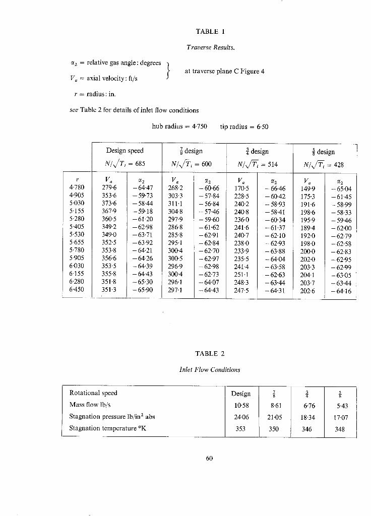
T A B L E 1
Traverse Results.
c~ z = r e l a t i ve gas a n g l e : d e g r e e s ~
Va = ax ia l v e l o c i t y : ft /s
r = r a d i u s : i n .
see T a b l e 2 for de t a i l s o f i n l e t f low c o n d i t i o n s
h u b r a d i u s = 4 .750
a t t r a v e r s e p l a n e C F i g u r e 4
t ip r a d i u s = 6.50
r
4.780
4.905
5.030
5.155
5-280
5.405
5.530
5.655
5.780
5.905
6.030
6.155
6.280
6.450
D e s i g n speed
N/x/~i = 685
Va 279.6
353.6
373.6
367.9
360.5
349.2
349.0
352.5
353.8
356-6
353.5
355.8
351.8
351.3
CX 2
- 64"47
- 5 9 " 7 3
- 58.44
- 5 9 " 1 8
- 6 1 ' 2 0
- 62"98
- 6 3 ' 7 1
- 63.92
- 64"21
- 6 4 ' 2 6
- 6 4 . 3 9
- 64 '43
- 65 '30
- 65 ' 90
~- d e s i g n
N/x//~ = 600
Va
268.2
303.3
311.1
304.8
297.9
286.8
285.8
295.1
300.4
300.5
296.9
300.4
296.1
297.1
0~ 2
- 60.66
- 57.84
- 56.84
- 57.46
- 59.60
- 61.62
- 62-91
- 62-84
- 62.70
- 62.97
- 62.98
- 62.73
- 64.07
- 64.43
_ 3 , d e s i g n
U/x/~i = 514
Va 170.5
228.5
240.2
240.8
236 '0
241.6
240.7
238"0
233"9
235"5
241.4
251"1
248.3
247.5
_Ss d e s i g n
N / ~ = 428
o~2 Va - 66 '46 149"9
- 60"42 175"3
- 5 8 " 9 3 191"6
- 58"41 198"6
- 60"34 195 '9
- 61"37 189 '4
- 6 2 " 1 0 192 '0
- 62"93 198 '0
- 63"88 200"0
- 64"04 202"0
- 63"58 203 '3
- 62"63 204 ' 1
- 63"44 203 '7
- 64"31 202 '6
O~ 2 - 65.04
- 61.45
- 58.99
- 58.33
- 59.46
- 62.00
- 62.79
- 62.58
- 62-83
- 62.95
- 62.99
- 63.05
- 63.44
- 6 4 . 1 6
T A B L E 2
Inlet Flow Conditions
R o t a t i o n a l speed
M a s s f low lb / s
S t a g n a t i o n p r e s s u r e l b / i n z a b s
S t a g n a t i o n t e m p e r a t u r e ° K
D e s i g n
10.58
24.06
353
7
8'61
21"05
350
3
6.76
18.34
346
5
5.43
17.07
348
60
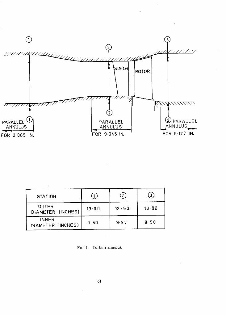
PARALLEL ANNULUS
FOR 2"065 IN.
PARALLEL ANNULUS
FOR 0.945 IN.
ROTOR
C ,)
" / / / / / / / / , ,,.,
\ \ \\\\\\\
( • PARALLEL
_=ANNULUS=_ FOR 6.127 IN.
STATION (~) (~)
OUTE~ ~3oo 12 $ 3 1~oo DIAMETER (INCHES)
INNER 9'50 9.97 9 '50
DIAMETER (INCHES)
FIG. 1. Turbine annulus.
61
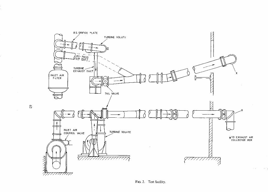
,S=•"?'°"•'•= ~<"'~ ,u=,,,N, vo,u,= !
/
k I I r~ , _ M ~ I I I ~f, .
/ / / / / / / / ~ / / /
I I ==- ~ / X
J / / / / / / / / / / / / / y////////,
~TO EXHAUST AIR COLLECTOR BOX
FIG. 2. Test facility.

1"01
O
<~
UJ r,- 1"0 - E~
ILl v...- (3.. 3 ; ILl
0 " 9 9 -
ixl _ J ~D Z <
h
1 0 -
_
- 1 0 -
1 " 2 -
o I - - < n."
>_ i > ~1"0 I-"- r j I::l
O > _..I LI..I
0 ' 8
4 " 5
H U B TIP
5.0 5.5 6"0
RADIUS
I TURBULENCE LEVEL 1.15% I FIG. 3. Turb ine inlet condit ions.
6 . 5
63
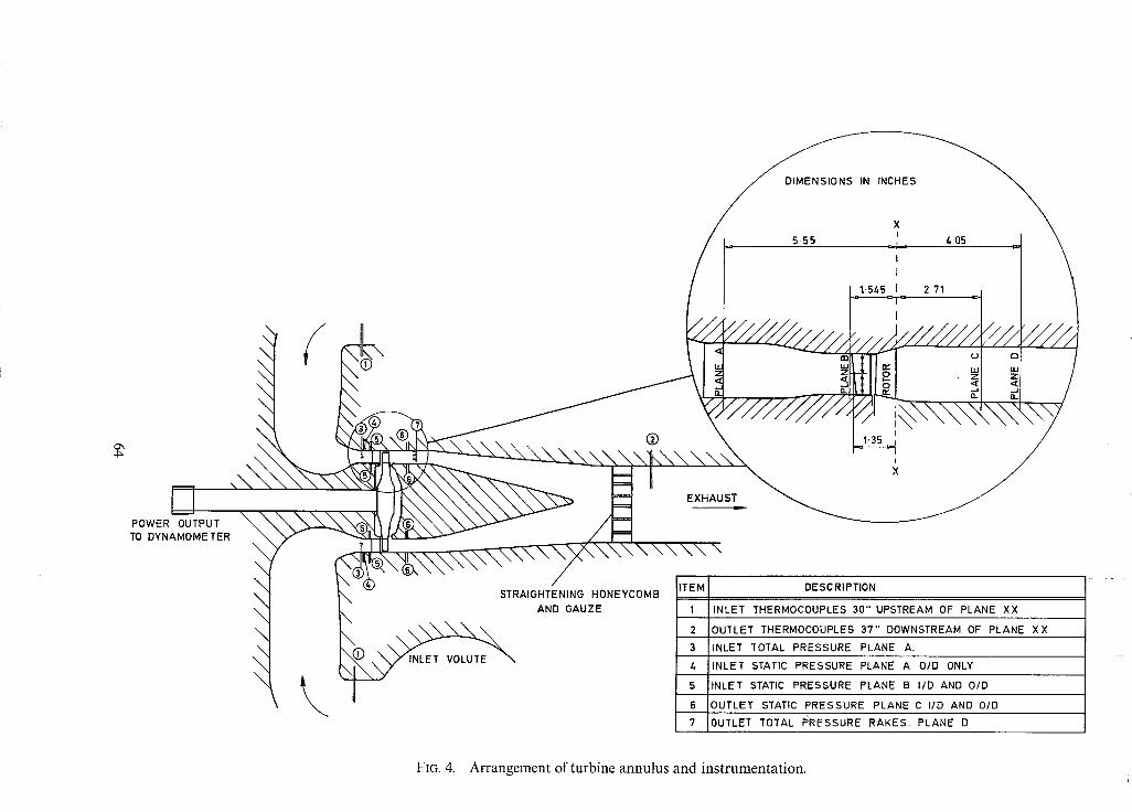
DIMENSIONS IN iNCHES
5.55
l'545 271
4.05
cP,
POWER OUTPUT TO DYNAMOMETER
\
\ \
\ \ \
\
\
\ INLET VOLUTE
®
STRAIGHTENING HONEYCOMB AND GAUZE
EXHAUST
O
ILl Z
. J I L
ITEM DESCRIPTION
1 INLET THERMOCOUPLES 30" UPSTREAM OF PLANE XX
2 OUTLET THERMOCOUPLES 37" DOWNSTREAM OF PLANE XX
3 INLET TOTAL PRESSURE PLANE A.
4 INLET STATIC PRESSURE PLANE A OlD ONLY
. 5 INLET STATIC PRESSURE PLANE B liD AND OlD
5 OUTLET STATIC PRESSURE PLANE C lID AND O/D
7 OUTLET TOTAL PRESSURE RAKES. PLANE D
FIG. 4. Arrangement of turbine annulus and instrumentation.
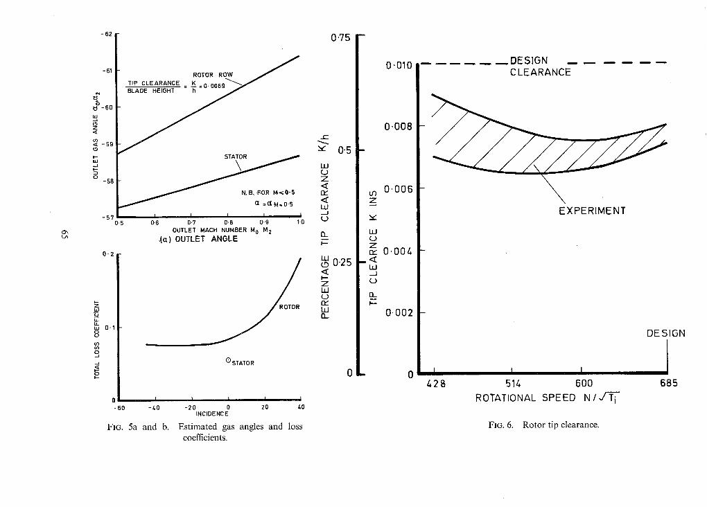
- 6 2 0-75
-61
~ - 6 0
O Z
.~ -59 o
i - 58
-5? 0-5
0'2
I L LL m 0.1 8
o,
o
ROTOR ROW J TIP CLEARANCE : ~=0.0069 ~ "
Z <
N.B, FOR M<0-5 t'Y
~ - a =aM:0.S < Ld I I I I I ._1
0.6 0.7 0-8 0.9 1-0 £") OUTLET MACH NUMBER M 0 M 2 EL
,(a) OUTLET ANGLE F--
< I,-- Z LU L.) rr" ILl n
Q STATO R
0 I -6o -40
FIG. 5a and b.
I I I I
-20 0 20 40 INCIDENCE
Estimated gas angles and loss coefficients.
0.010
0.25
m
0-5 -
U3 Z
LLI (.9
_ < UJ
(....)
13_ I-,.
0 -
0 . 0 0 8
0 . 0 0 6 \ E X P E R I M E N T
0.004
0 0 0 2
0
D E S I G N _ _ .
C L E A R A N C E
D E S I G N
4 2 8 514 600
ROTATIONAL SPEED NIJT i
685
FIG. 6. Rotor tip clearance.

95
E
> 90 Z U.I ¢D
t L U_ LU
85
95
>- 90 (..5 Z I.U
1L LL
w 8 5
95
E
9O Z [.u
G LL I I IL l
85 0'8
DESIGN LOADING
w - -
(a) BRAKE MEASURED
e ~'~e
FIG. 7.
(b) BRAKE CONTINUITY I I I I
I PREDICTED Q-- -@ EXPERIMENT
(c) COUPLES MEASURED
t I I I
1"0 1"2 1"/, 1"6 KpAT
STAGE LOADING U2 m
Stage efficiency - design speed, N / x / ~ i = 685.
8.5
~ 8-0
ffl <
7-5 1"/,
/
f
I ( ~E ) ' ' ®
DESIGN LOADING
o ® _ .,,,.G(9,-- "E~ ~
I i I I I 1.5 1.6 1-7 1.8 1-9
STAGE TOTAL PRESSURE RATIO Pim/P3c
PREDICTED [
®~- -®- -@ EXPERIMENT
.•1.6 Cr"
.s " ' G 1.4
1.2
1.0
0.8
FIG. 8. Swallowing capacity and stage loading
design speed, N / x / ~ i = 685.
E : 3
O Z Q .< o
LU '.9 g ' l
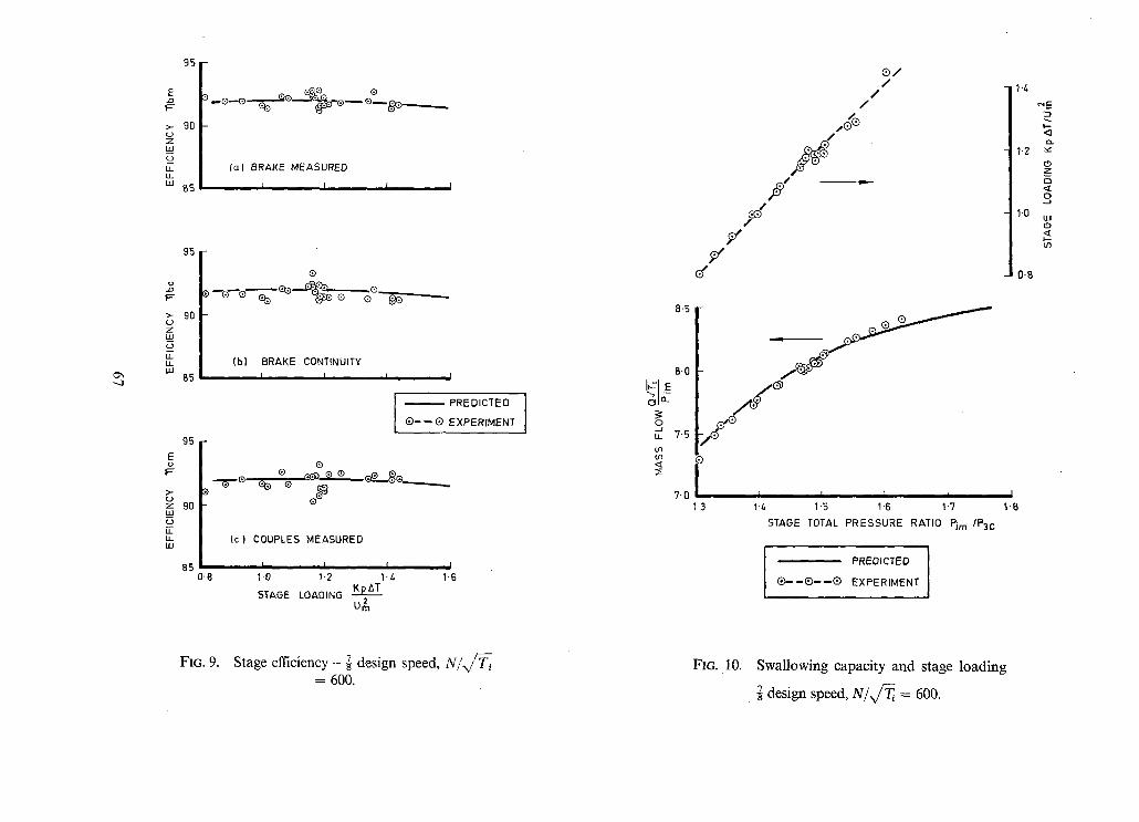
, , . j
95
E #
>- 90 z
LI_
tu B5
I F
9o
w B5
95 E #
>- t j z 90
u_ 11- t..(J
85
@' ®
--e--e ee Q e - - - ~ - e - - e - - ~ ~
(a) BRAKE MEASURED I I I I
@
(b) BRAKE CONTINUITY l I f I
[ ~ P R E D I C T E D I ® - - @ EXPERIMENT
O
- e "e % e e ~
(c) COUPLES MEASURED
I I I , I 0"8 1"0 1-2 1"" 1"6
STAGE LOADING KpAT u~
FIG. 9. Stage efficiency - ~- des ign speed, N/,~i = 600.
8'5
B-0
O _J ,, 7'5 U3 U~ <l. :E
7'
7 - 0 L - 1 3
0 / / /
/
/ J /
Y
f °
1./,
1-2
1.g
0-B
1/ , 1-5 1-6 1-7
STAGE TOTAL PRESSURE RATIO Pim /P3c
J PREDICTED I
~E~-. -®----0 EXPERIMENT
1.B
FIG. 10. Swallowing capacity and stage loading
~- design speed, N/x//~i = 600.
"E
~c
O Z 1"7
..9 ° ILl LR,
U3
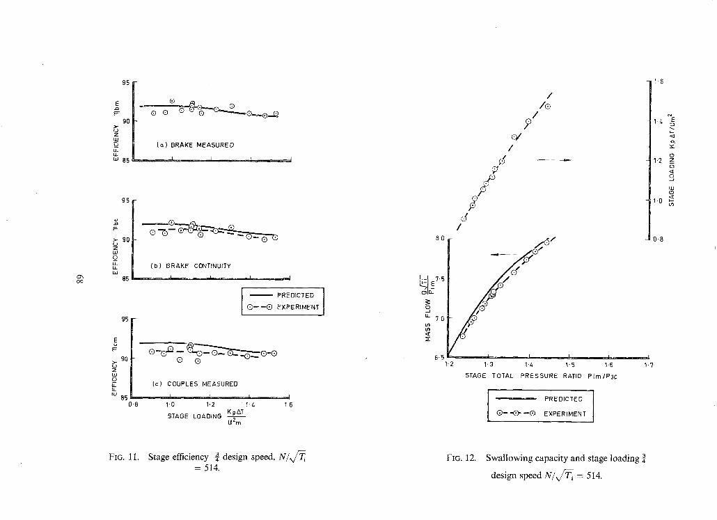
o', ,30
95
E
90
uJ 85
®
le ) BRAKE MEASURED
J I L J
95
F
>- 90 (J z U LL LL LU
85
{b) BRAKE CONTINUITY
! I t I
(~)-- --@ EXPERIMENT
95
E F
90
7
(-2
LU B5
0.8
® ®
(c) COUPLES MEASURED
i I I
1-0 1.2 l. t ,
STAGE LOADING KpAT U2m
I 1-6
FIG. 11. Stage efficiency-¼ design speed, N/xf-~i = 514.
8-0
[~ E 7"5 o/ff
o _J
u_ 7.0 (/1
~r
6"5 1'2
/
/ P
c/ /
c¢ /
®,-
I
1.3
STAGE TOTAL
I t I
1"4 1'5 1"6
PRESSURE RATIO P im/P3c
® - -E)- --(Z) PREDICTED I
EXPERIMENT
FIG. 12. Swallowing capacity and stage loading 3
design speed N/,~ii = 514.
1 ' 6
1.2 _z o
£ uJ o <
1.[1 B.- m
0"8
I 1"7

~D
95
E
F"
,~ 90 Z Lu _u i i I i LU
85
9 6
F
9o Z ~u
U_ i i I.U
85
95
E u
> -
90 t U
LI_ Ix. t U
85 0
FIG. 13.
® (D o
(o) BRAKE MEASURED
I I I
®
_.. ® ®®
N ® ~ - - . . . ® _ ®
( b ) B R A K E CONTINUTY
I I I I
- - PREDICTED
G - - - - G EXPERIMENT
(c) COUPLES MEASURED
1 I I 1.2 1-,'- 1"6
I I"B
Stage efficiency ~- design s p e e d , N/~i = 428.
7-5
~ E ? ' 0
o, LL
6.5 (/3 ~q <
6'0 1'1
$
/ ®
!
I
¢ /
S /
/ o
? /
t I I I 1"2 1.3 l '& 1"5
STAGE TOTAL PRESSURE RATIO P i m / P 3 c
PREDICTED
~ - , -E~, - - O EXPERIMENT
1"8
1"6
0 _
1"4 o,
1.2 ~
1.0
t 1"6
FIG. 14. Swallowing capacity and stage loading ~-
design speed N/~i = 428.
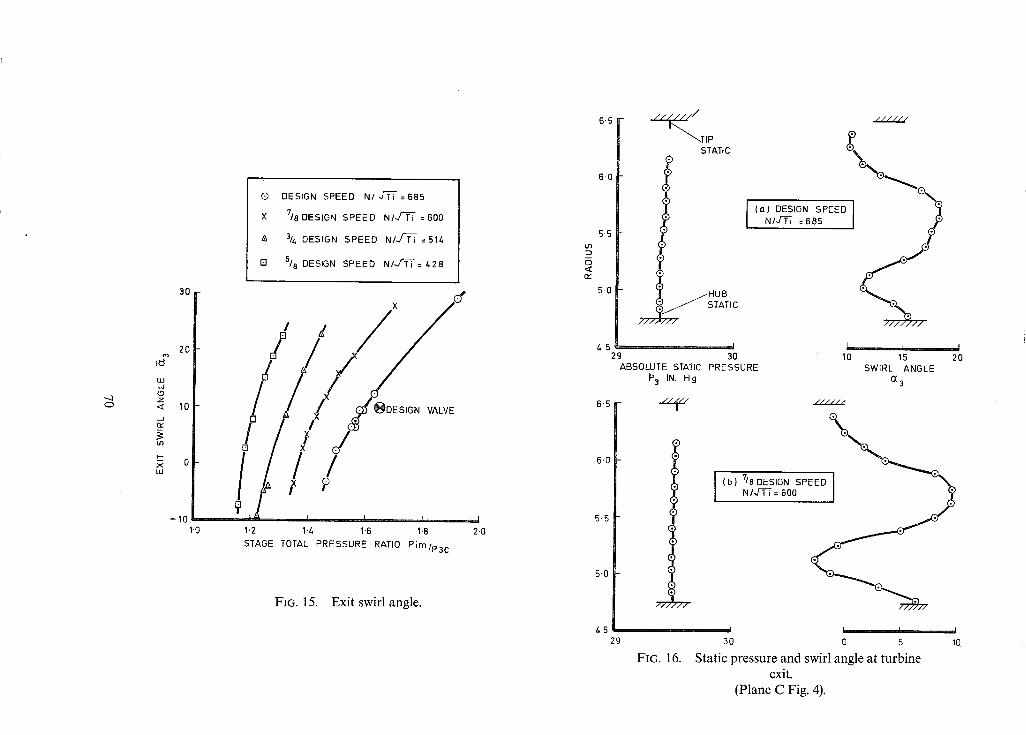
"--...I
,J I.IJ _J
z <
f f l
i - -
x w
30
20
10
- 1 0 1"0
E) DESIGN SPEED N/ ~ =685
X 7/8 DESIGN SPEED N/,/~'T = 600
A 314 DESIGN SPEED N/.../ '~ = 51/.,
[] 5/8 DESIGN SPEED N / H = / , 2 8
1.2 14 1'6 1-8 2-0 STAGE TOTAL PRESSURE RATIO P im/p3c
FIG. 15. Exit swirl angle.
6-5 - g - ~ / '"'"'-.TIP
STATIC
6.0 (~ ®
5-0 / H U B / S T A T I C
Y77 777"
4"5 I 29 30
ABSOLUTE STATIC PRESSURE I' 3 IN. H g
6"5
5-5
: : 3
n,-"
6.0
5.5
5.0
/ / , / f
4'5
l i t ' g i g
\ [a ) DESIGN SPEED I
N / . / - ~ = 6 8s I
/ I / / / / ' /
[,1 t t
10 15 20 SWIRL ANGLE
(13 / / / / / ' /
1 ~ I . I I
29 30 0 5 10
FIG. 16. Static pressure and swirl angle at turbine exit.
(Plane C Fig. 4).
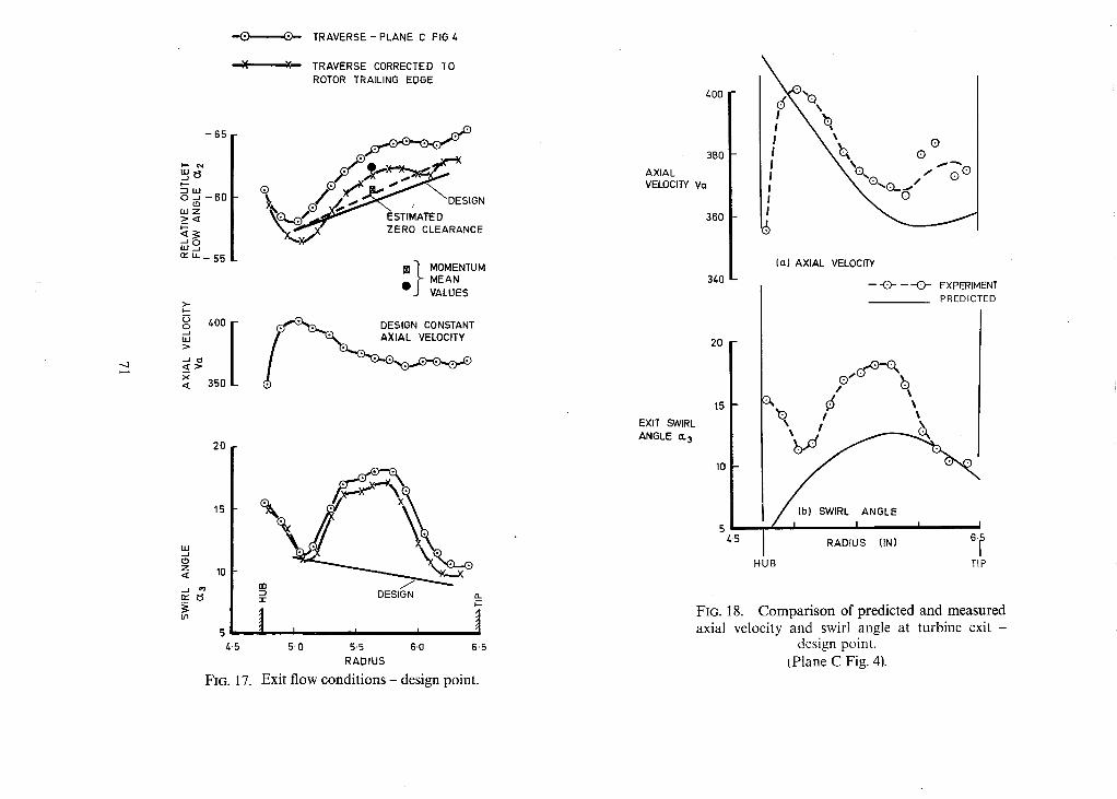
X
G),-, TRAVERSE - PLANE C FIG 4.
X~ TRAVERSE CORRECTED TO ROTOR TRAILING EDGE
- 6 5
F. -
, ~ , -60 4_~
L U Z
,_.1
n." u__ 55
>-
o ~ 4.00 [ LU
x < 350
(~7~G)N..G ~ ESTIMATE ~ ~ G N ~,w.-,'~'-x/X " ZERO CLEARANCE
} MOMENTUM MEAN VALUES
DESIGN CONSTANT
ILl .--I 0 Z
2O
10 r a
DESIGN ~. - r F---
t - 5 5-0 5"5 6"0 6"5 RADIUS
FIG. 17. Exit flow conditions - design point.
400 ! "
380 -
AXIAL VELOCITY V,',
360
340
20
15 EXIT SWIRL ANGLE (:c 3
10
5 4-5
I I ! O
(a) AXIAL VELOCITY
-- -'O-- -- -O- EXPERIMENT PREDICTED
lib) SWIRL IANGLE I I
RADIUS (IN) 6" I
HUB TIP
FIG. 18. Comparison of predicted and measured axial velocity and swirl angle at turbine exit -
design point. (Plane C Fig. 4).
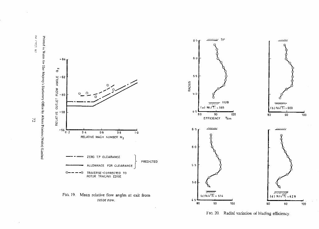
-..j
.~.
,7
O
©
>
E == '-o
.~.
-64
g
-62 r_~ Z
o, LL --60
._1
0
-58 >
C~
-56 0-2
I I p • 0'4 0"6 08 1"0
RELATIVE MACH NUMBER M 2
ZERO TIP CLEARANCE t PREDICTED
ALLOWANCE FOR CLEARANCE
~--I.Q TRAVERSE-CORRECTED TO ROTOR TRAILING EDGE
FIG. 19. Mean relative flow angles at exit from rotor row.
O
rY
6.5
6.0
5"5
5.0
z,.5
/ / / / / / / / / TIP
HUB / i / / / / /
lea) N/,J'Ti = 685 I
8O 9O 100 EFFICIENCY ~cm
/ / / / / /
/ / / / / / /
b) NL/-T'~ = 600 I I
80 90 100
6'5
6"0
5"5
5.0
4.5 80
/ / / / / / /
( II//I/
(c) NIJ-~" = 51~ I I
90 100
///////
///////I/
[d) Nl,,,r~ = 4 2 8
BO 90 100
FIG. 20. Radial variation of blading efficiency.

R. & M. No. 354
© Crown copyright 1968
Published by HER MAJESTY'S STATIONERY OFFICE
To be purchased from 49 High Holborn, London w.c. 1 423 Oxford Street, London w. 1 13A Castle Street, Edinburgh 2
109 St. Mary Street, Cardiff CF1 1JW Brazennose Street, Manchester 2
50 Fairfax Street, Bristol BS I 3DE " 258.-259 Broad Street, Birmingham 1
7-11 Linenhall Street, Belfast BT2 8AY or through any bookseller
R. & M. No. 3541 S.O. Code No. 23 3541


