1
Introduction to Electronic Design Automation
Jie-Hong Roland Jiang江介宏
Department of Electrical EngineeringNational Taiwan University
Spring 2011
2
Model of Computation

3
Model of Computation In system design, intended system behavior is translated
into physical implementation The physical implementation can be in hardware or software,
in silicon or non-silicon (e.g., living cells) How a system behaves or interacts with its environmental
stimuli must be specified formally
Model of computation (MoC) can be seen as the subject of devising/selecting effective “data structures” in describing system behaviors precisely and concisely
MoC gives a formal way of describing system behaviors It is useful in the specification, synthesis and verification of
systems
4
Model of Computation
Outline State transition systems
Finite automata / finite state machines Real-time systems
Timed automata Hybrid systems
Hybrid automata for hybrid systems, which exhibits both discrete and continuous dynamic behavior
Asynchronous systemsPetri nets for asynchronous handshaking
Signal processing systemsDataflow process network for signal processing applications
(See Wikipedia for more detailed introduction)
5
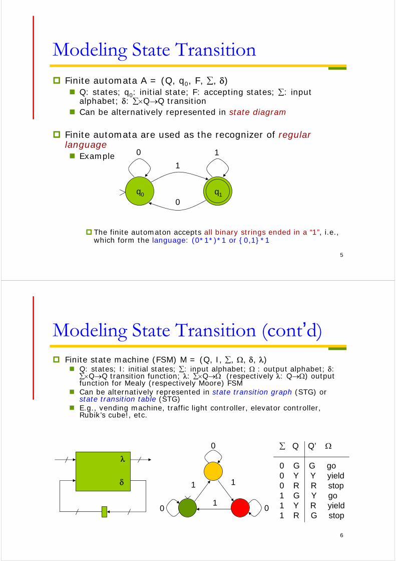
Modeling State Transition Finite automata A = (Q, q0, F, , )
Q: states; q0: initial state; F: accepting states; : input alphabet; : QQ transition
Can be alternatively represented in state diagram
Finite automata are used as the recognizer of regular language Example
The finite automaton accepts all binary strings ended in a “1”, i.e., which form the language: (0*1*)*1 or {0,1}*1
1
1
0
0
q0 q1
6
Modeling State Transition (cont’d) Finite state machine (FSM) M = (Q, I, , , , )
Q: states; I: initial states; : input alphabet; : output alphabet; : QQ transition function; : Q (respectively : Q) output function for Mealy (respectively Moore) FSM
Can be alternatively represented in state transition graph (STG) or state transition table (STG)
E.g., vending machine, traffic light controller, elevator controller, Rubik’s cube!, etc.
1
1
1
00
0 Q Q’
0 G G go0 Y Y yield0 R R stop1 G Y go1 Y R yield1 R G stop
7
Modeling State Transition (cont’d)
FSMs are often used as controllers in digital systems E.g. data flow controller, ALU (arithmetic logic
unit) controller, etc.
Variants of FSMHierarchical FSMCommunicating FSM …
8
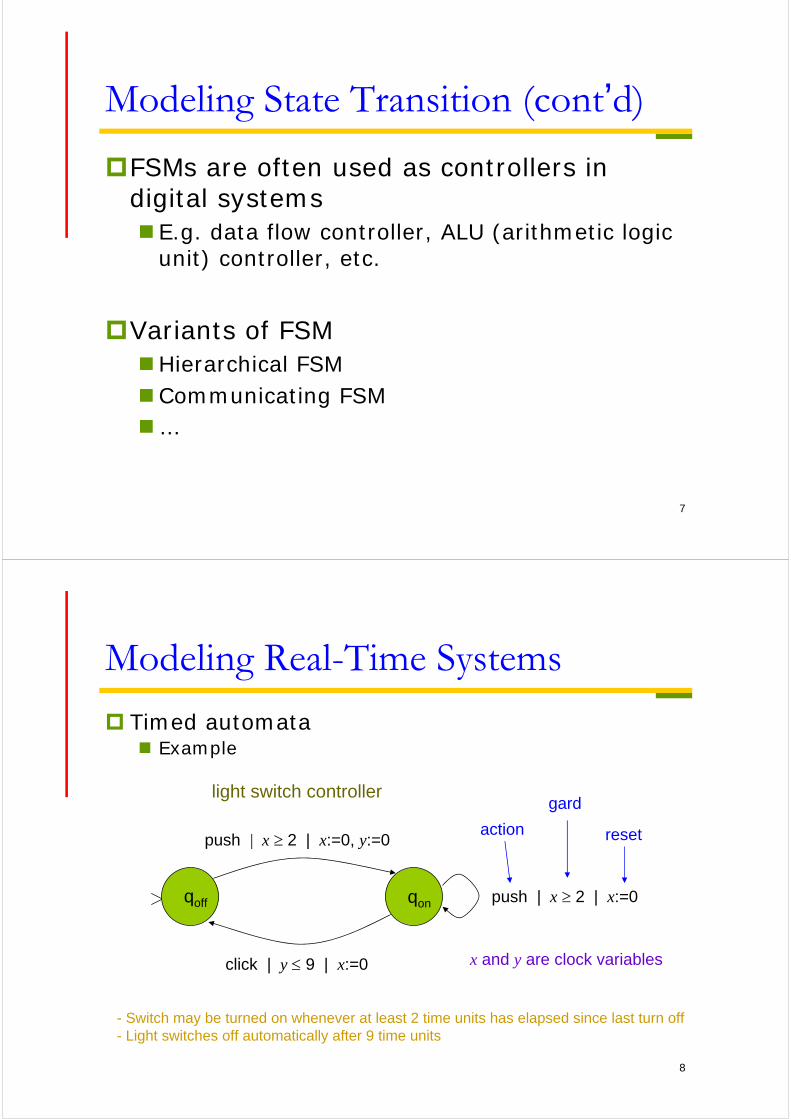
Modeling Real-Time Systems
Timed automata Example
push | x 2 | x:=0, y:=0
click | y 9 | x:=0
qoff qon
light switch controller
push | x 2 | x:=0
x and y are clock variables
- Switch may be turned on whenever at least 2 time units has elapsed since last turn off- Light switches off automatically after 9 time units
action
gard
reset
9
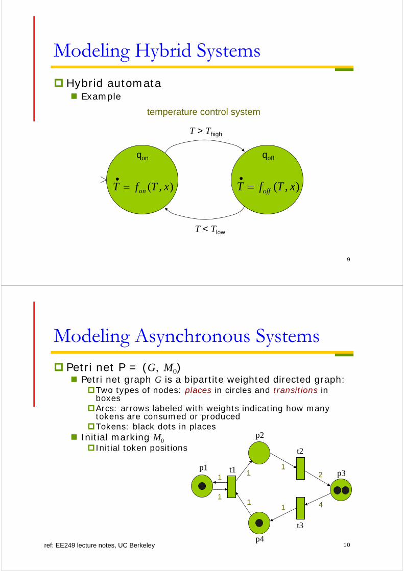
Modeling Hybrid Systems
Hybrid automata Example
( , )onT f T x ( , )offT f T x
T > Thigh
T < Tlow
temperature control system
qon qoff
10
Modeling Asynchronous Systems
Petri net P = (G, M0) Petri net graph G is a bipartite weighted directed graph:
Two types of nodes: places in circles and transitions in boxes
Arcs: arrows labeled with weights indicating how many tokens are consumed or produced
Tokens: black dots in places Initial marking M0
Initial token positions
t1p1
p2
t2
p3
t3
p4
1
1
1
1
2
4
1
1
ref: EE249 lecture notes, UC Berkeley
11
Modeling Asynchronous Systems (cont’d)
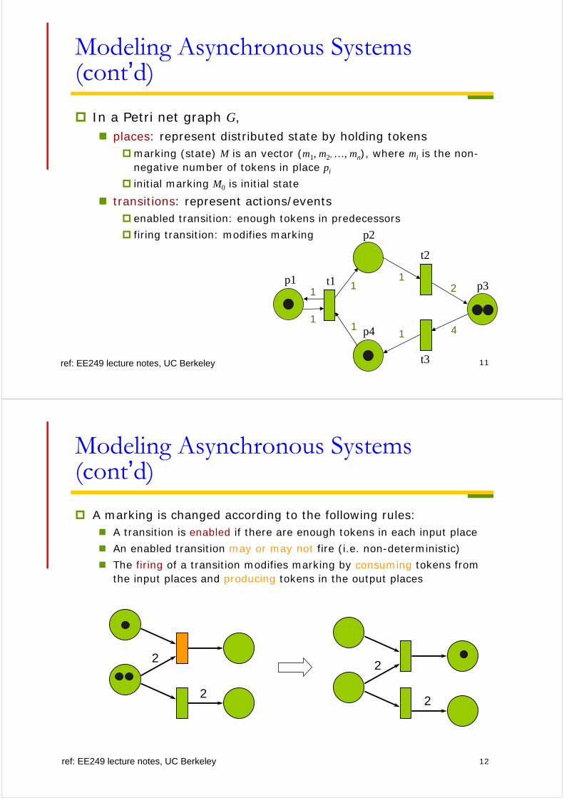
In a Petri net graph G, places: represent distributed state by holding tokens
marking (state) M is an vector (m1, m2, …, mn), where mi is the non-negative number of tokens in place pi
initial marking M0 is initial state
transitions: represent actions/events enabled transition: enough tokens in predecessors
firing transition: modifies marking
t1p1
p2
t2
p3
t3
p4
1
1
1
1
2
4
1
1
ref: EE249 lecture notes, UC Berkeley
12
Modeling Asynchronous Systems (cont’d)
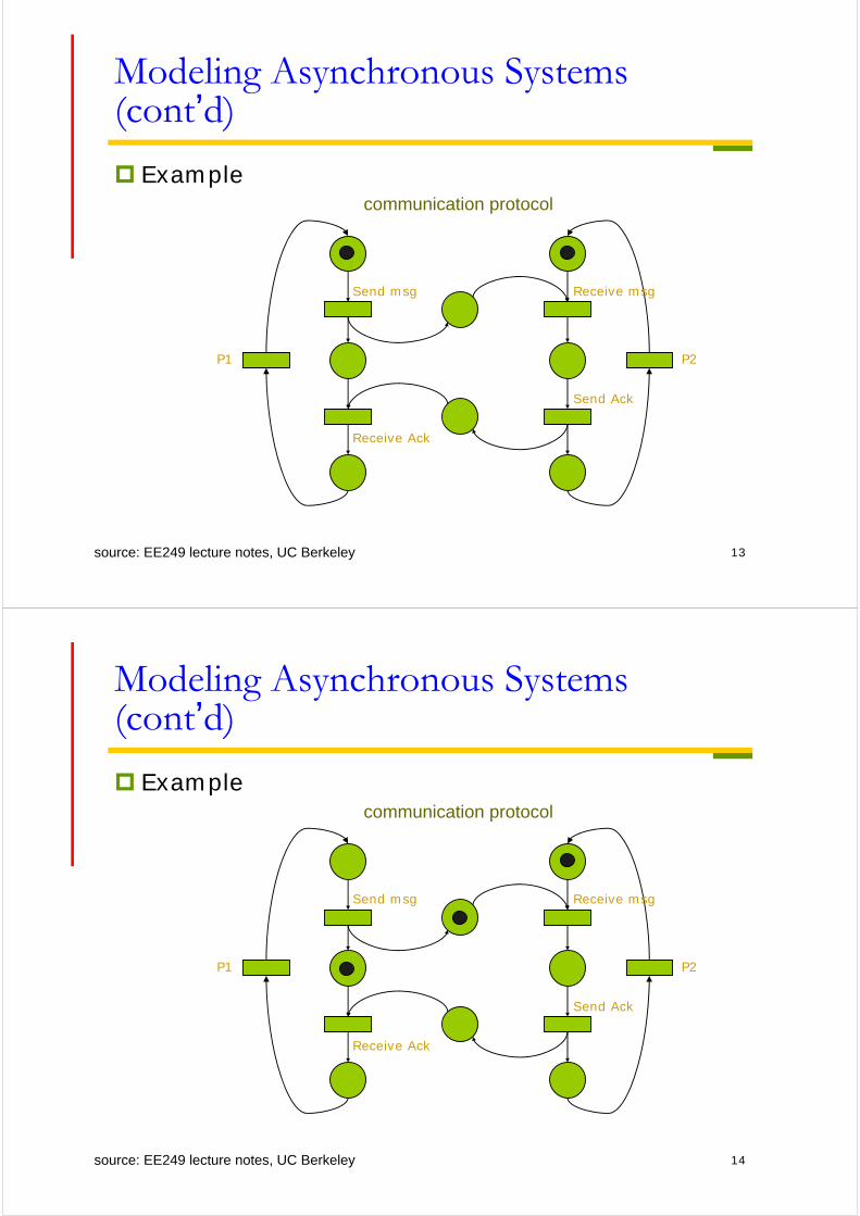
A marking is changed according to the following rules: A transition is enabled if there are enough tokens in each input place
An enabled transition may or may not fire (i.e. non-deterministic)
The firing of a transition modifies marking by consuming tokens from the input places and producing tokens in the output places
22
22
ref: EE249 lecture notes, UC Berkeley
13
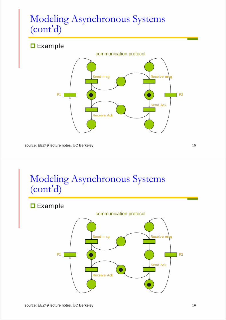
Modeling Asynchronous Systems (cont’d)
Examplecommunication protocol
P1
Send msg
Receive Ack
Send Ack
Receive msg
P2
source: EE249 lecture notes, UC Berkeley
14
Modeling Asynchronous Systems (cont’d)
Examplecommunication protocol
P1
Send msg
Receive Ack
Send Ack
Receive msg
P2
source: EE249 lecture notes, UC Berkeley
15
Modeling Asynchronous Systems (cont’d)
Examplecommunication protocol
P1
Send msg
Receive Ack
Send Ack
Receive msg
P2
source: EE249 lecture notes, UC Berkeley
16
Modeling Asynchronous Systems (cont’d)
Examplecommunication protocol
P1
Send msg
Receive Ack
Send Ack
Receive msg
P2
source: EE249 lecture notes, UC Berkeley

17
Modeling Asynchronous Systems (cont’d)
Examplecommunication protocol
P1
Send msg
Receive Ack
Send Ack
Receive msg
P2
source: EE249 lecture notes, UC Berkeley
18
Modeling Asynchronous Systems (cont’d)
Examplecommunication protocol
P1
Send msg
Receive Ack
Send Ack
Receive msg
P2
source: EE249 lecture notes, UC Berkeley

19
Modeling Signal Processing Data-flow process network
Nodes represent actors; arcs represent FIFO queues Firing rules are specified on arcs Actors respect firing rules that specify how many tokens must be
available on every input for an actor to fire. When an actor fires, it consumes a finite number of tokens and produces also a finite number of output tokens.
1
1
2
2
1
1
ref: http://www.create.ucsb.edu/~xavier/Thesis/html/node38.html
20
MoC in System Construction
There are many other models of computation tailored for specific applications Can you devise a new computation model in some
domain?
Hierarchical modeling combined with several different models of computation is often necessary
By using a proper MoC, a system can be specified formally, and further synthesized and verified In the sequel of this course, we will be focusing on FSMs
mainly

21
High Level Synthesis
Logic synthesis
High-level synthesis
Physical design
Slides are by Courtesy of Prof. Y.-W. Chang
22
High Level Synthesis
Course contentsHardware modelingData flowScheduling/allocation/assignment
ReadingChapter 5
23
High Level Synthesis Hardware-description language (HDL) synthesis
Starts from a register-transfer level (RTL) description; circuit behavior in each clock cycle is fixed
Uses logic synthesis techniques to optimize the design Generates a netlist
High-level synthesis (HLS), also called architectural or behavioral synthesis Starts from an abstract behavioral description Generates an RTL description It normally has to perform the trade-off between the
number of cycles and the hardware resources to fulfill a task
24
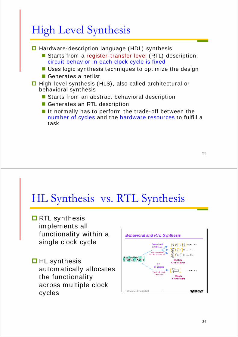
HL Synthesis vs. RTL Synthesis
RTL synthesis implements all functionality within a single clock cycle
HL synthesis automatically allocates the functionality across multiple clock cycles
25
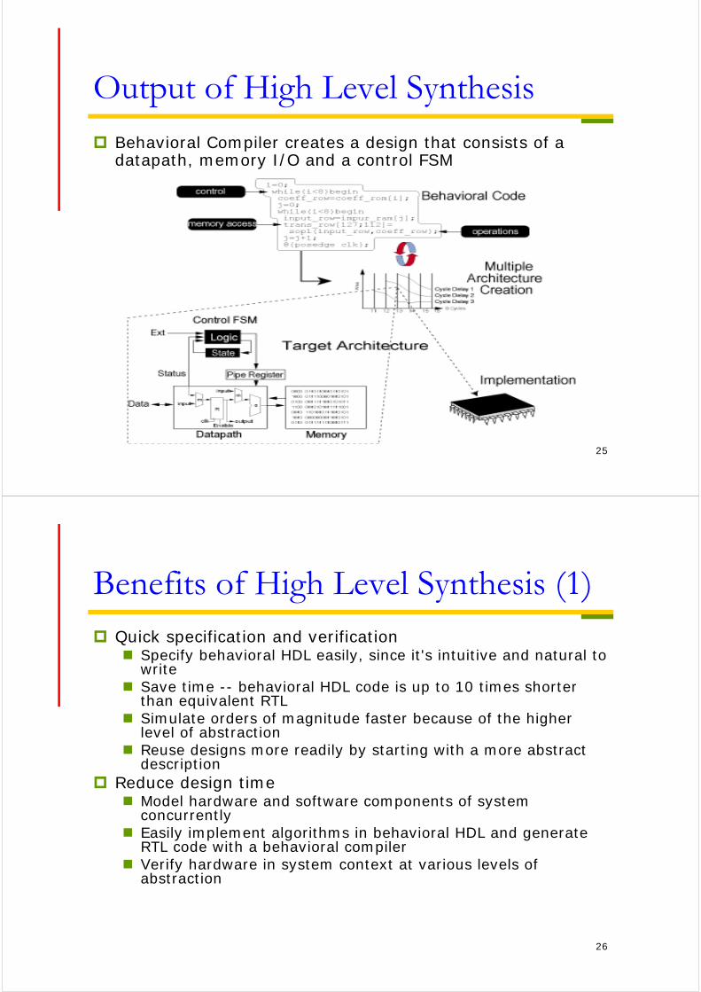
Output of High Level Synthesis Behavioral Compiler creates a design that consists of a
datapath, memory I/O and a control FSM
26
Benefits of High Level Synthesis (1) Quick specification and verification
Specify behavioral HDL easily, since it's intuitive and natural to write
Save time -- behavioral HDL code is up to 10 times shorter than equivalent RTL
Simulate orders of magnitude faster because of the higher level of abstraction
Reuse designs more readily by starting with a more abstract description
Reduce design time Model hardware and software components of system
concurrently Easily implement algorithms in behavioral HDL and generate
RTL code with a behavioral compiler Verify hardware in system context at various levels of
abstraction
27
Benefits of High Level Synthesis (2)
Explore architectural trade-offs Create multiple architectures from a single specification Trade-off throughput and latency using high-level
constraints Analyze various combinations of technology-specific
datapath and memory resources Evaluate cost/performance of various implementations
rapidly Automatically infer memory and generate FSM
Specify memory reads and writes Schedule memory I/O, resolve conflicts by building
control FSM Trade-off single-ported (separate registers) vs. multi-
ported memories (register files) Generate a new FSM
28
Hardware Models for HL Synthesis All HLS systems need to restrict the target hardware
Otherwise search space is too large All synthesis systems have their own peculiarities, but most
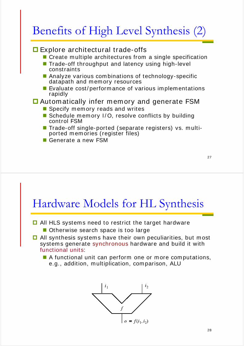
systems generate synchronous hardware and build it with functional units: A functional unit can perform one or more computations,
e.g., addition, multiplication, comparison, ALU
29
Hardware Models
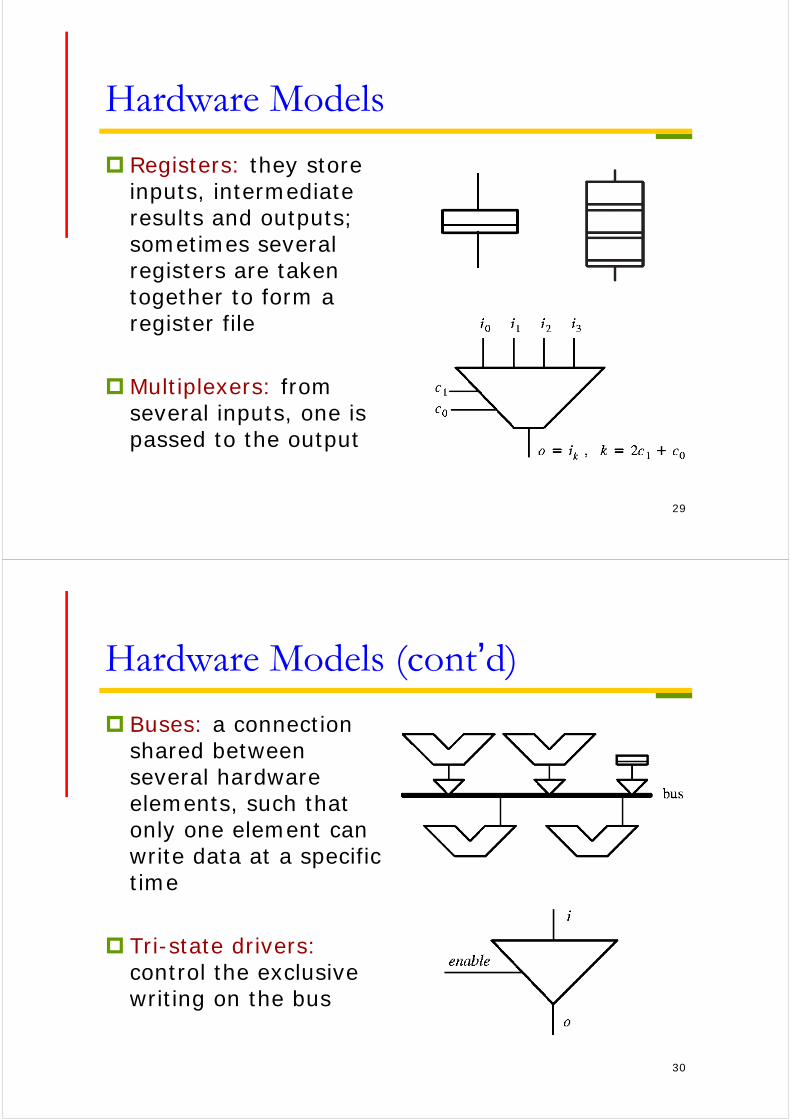
Registers: they store inputs, intermediate results and outputs; sometimes several registers are taken together to form a register file
Multiplexers: from several inputs, one is passed to the output
30
Hardware Models (cont’d)
Buses: a connection shared between several hardware elements, such that only one element can write data at a specific time
Tri-state drivers:control the exclusive writing on the bus
31
Hardware Models (cont’d)
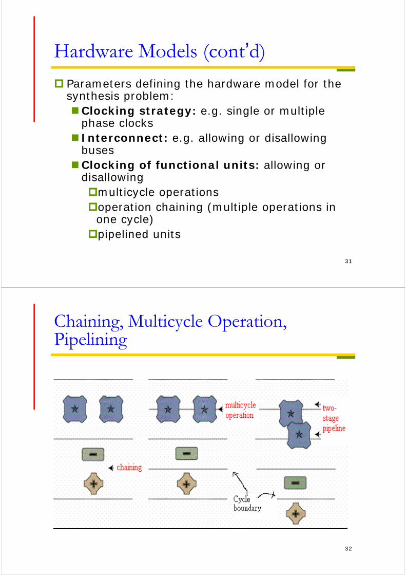
Parameters defining the hardware model for the synthesis problem:Clocking strategy: e.g. single or multiple
phase clocks Interconnect: e.g. allowing or disallowing
busesClocking of functional units: allowing or
disallowingmulticycle operationsoperation chaining (multiple operations in
one cycle)pipelined units
32
Chaining, Multicycle Operation, Pipelining
33
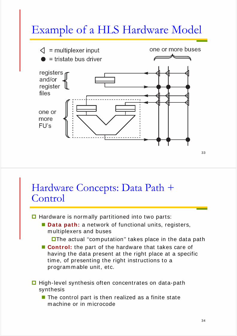
Example of a HLS Hardware Model
34
Hardware Concepts: Data Path + Control
Hardware is normally partitioned into two parts: Data path: a network of functional units, registers,
multiplexers and busesThe actual ‘‘computation’’ takes place in the data path
Control: the part of the hardware that takes care of having the data present at the right place at a specific time, of presenting the right instructions to a programmable unit, etc.
High-level synthesis often concentrates on data-path synthesis The control part is then realized as a finite state
machine or in microcode
35
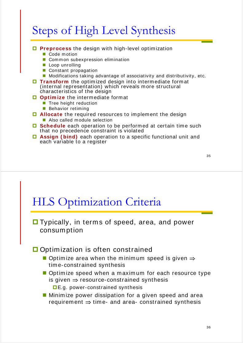
Steps of High Level Synthesis Preprocess the design with high-level optimization
Code motion Common subexpression elimination Loop unrolling Constant propagation Modifications taking advantage of associativity and distributivity, etc.
Transform the optimized design into intermediate format (internal representation) which reveals more structural characteristics of the design
Optimize the intermediate format Tree height reduction Behavior retiming
Allocate the required resources to implement the design Also called module selection
Schedule each operation to be performed at certain time such that no precedence constraint is violated
Assign (bind) each operation to a specific functional unit and each variable to a register
36
HLS Optimization Criteria
Typically, in terms of speed, area, and power consumption
Optimization is often constrained Optimize area when the minimum speed is given
time-constrained synthesis Optimize speed when a maximum for each resource type
is given resource-constrained synthesisE.g. power-constrained synthesis
Minimize power dissipation for a given speed and area requirement time- and area- constrained synthesis
37
Input Format
The algorithm, which is the input to a high-level synthesis system, is often provided in textual form either in a conventional programming language, such
as C, C++, SystemC, or in a hardware description language (HDL),
which is more suitable to express the parallelism present in hardware.
The description has to be parsed and transformed into an internal representation and thus conventional compiler techniques can be used.
38
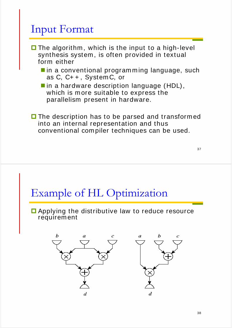
Example of HL Optimization
Applying the distributive law to reduce resource requirement
39
Internal Representation
Most systems use some form of a data-flow graph (DFG) A DFG may or may not
contain information on control flow
A data-flow graph is built from vertices (nodes):
representing computation, and
edges: representing precedence relations
40
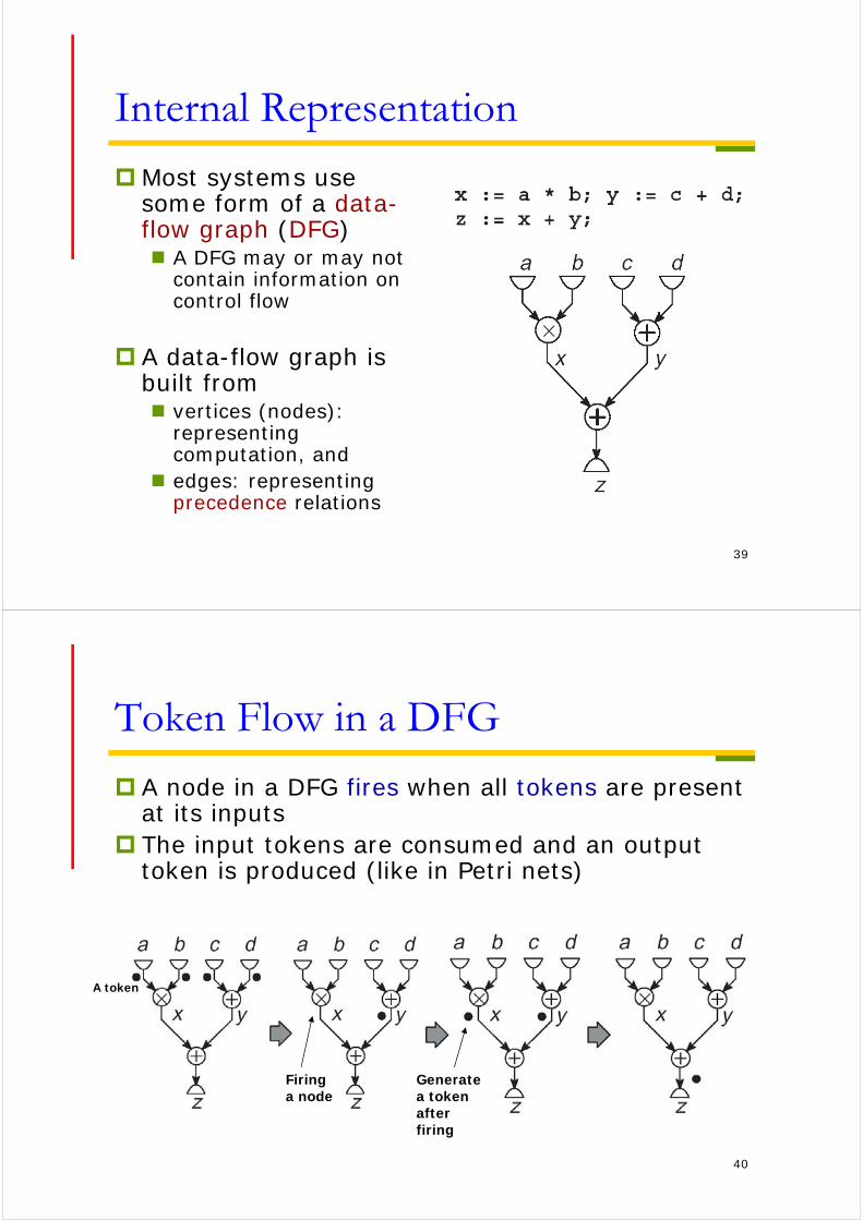
Token Flow in a DFG
A node in a DFG fires when all tokens are present at its inputs
The input tokens are consumed and an output token is produced (like in Petri nets)
A token
Firing a node
Generate a token after firing
41
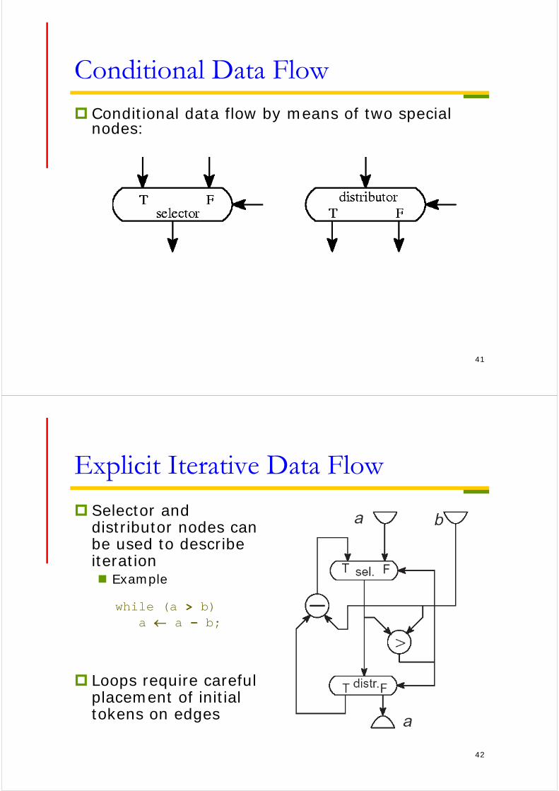
Conditional Data Flow
Conditional data flow by means of two special nodes:
42
Explicit Iterative Data Flow
Selector and distributor nodes can be used to describe iteration Example
Loops require careful placement of initial tokens on edges
while (a > b)a a – b;
43
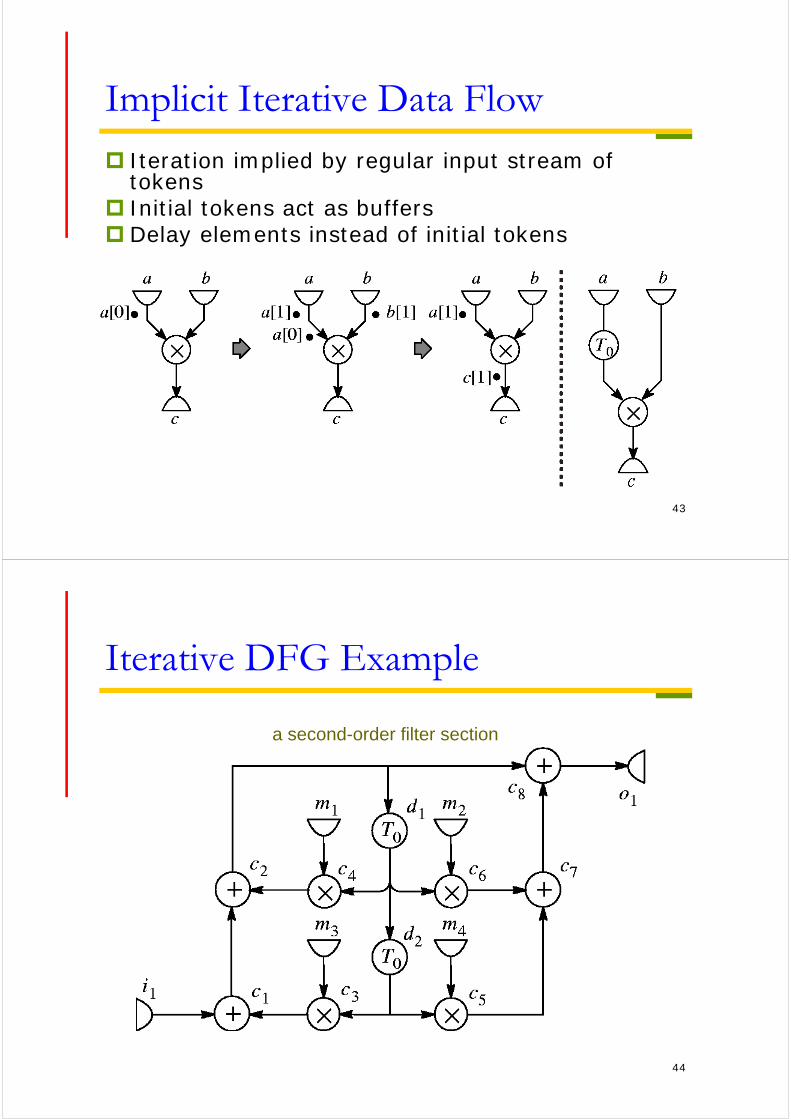
Implicit Iterative Data Flow
Iteration implied by regular input stream of tokens
Initial tokens act as buffers Delay elements instead of initial tokens
44
Iterative DFG Example
a second-order filter section
45
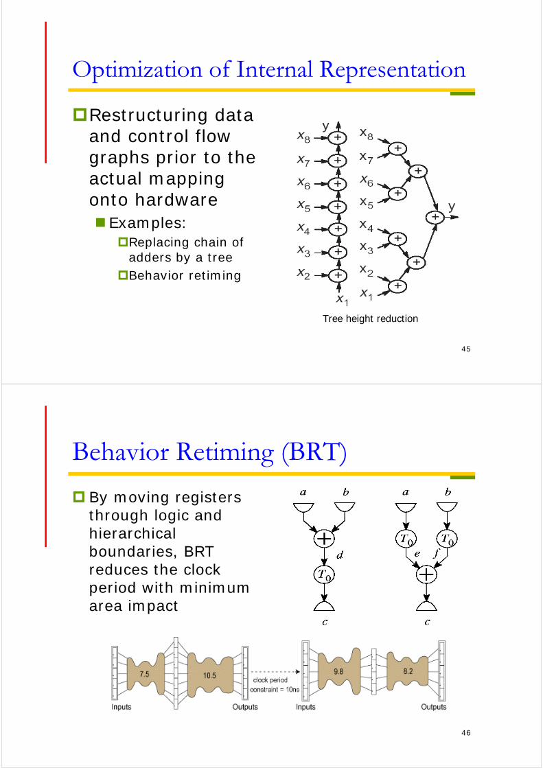
Optimization of Internal Representation
Restructuring data and control flow graphs prior to the actual mapping onto hardware Examples:
Replacing chain of adders by a tree
Behavior retiming
Tree height reduction
46
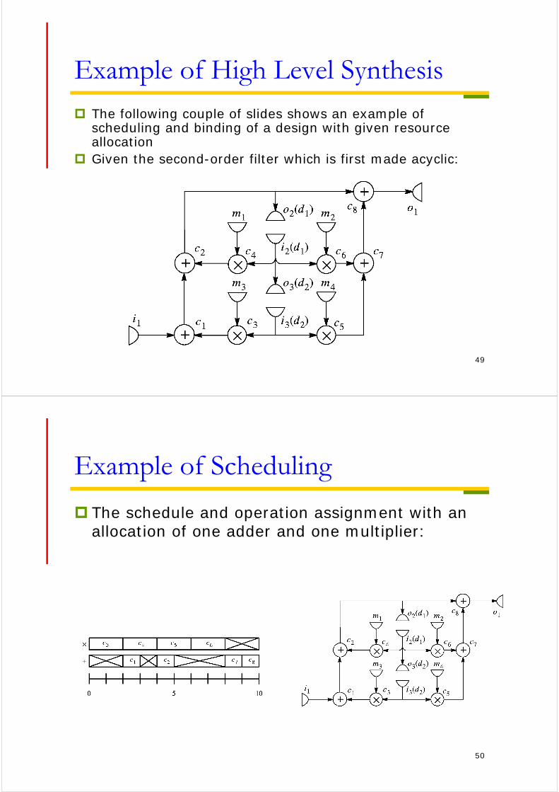
Behavior Retiming (BRT)
By moving registers through logic and hierarchical boundaries, BRT reduces the clock period with minimum area impact

47
Effectiveness of Behavior Retiming
RTL designs have a single clock net and were synthesized into gates using Synopsys Design Compiler
Design type: dataflow implies significant number of operators; control implies state machine dominated
Synopsys exp:
48
HLS Subtasks: Allocation, Scheduling, Assignment
Subtasks in high-level synthesis Allocation (Module selection): specify the hardware
resources that will be necessary Scheduling: determine for each operation the time at which it
should be performed such that no precedence constraint is violated
Assignment (Binding): map each operation to a specific functional unit and each variable to a register
Remarks: Though the subproblems are strongly interrelated, they are
often solved separately. However, to attain a better solution, an iterative process executing these three subtasks must be performed.
Most scheduling problems are NP-complete heuristics are used
49
Example of High Level Synthesis The following couple of slides shows an example of
scheduling and binding of a design with given resource allocation
Given the second-order filter which is first made acyclic:
50
Example of Scheduling
The schedule and operation assignment with an allocation of one adder and one multiplier:
51
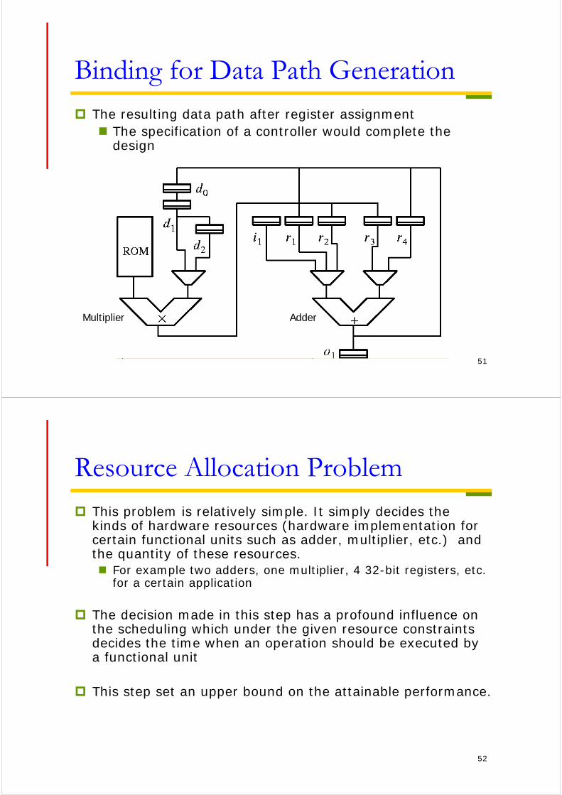
Binding for Data Path Generation The resulting data path after register assignment
The specification of a controller would complete the design
Multiplier Adder
52
Resource Allocation Problem This problem is relatively simple. It simply decides the
kinds of hardware resources (hardware implementation for certain functional units such as adder, multiplier, etc.) and the quantity of these resources. For example two adders, one multiplier, 4 32-bit registers, etc.
for a certain application
The decision made in this step has a profound influence on the scheduling which under the given resource constraints decides the time when an operation should be executed by a functional unit
This step set an upper bound on the attainable performance.

53
Problem Formulation of Scheduling Input consists of a DFG G(V, E) and a library of resource
types There is a fixed mapping from each v V to some r ;
the execution delay (v) for each operation is therefore known
The problem is time-constrained; the available execution times are in the set
A schedule :VT maps each operation to its starting time; for each edge (vi, vj) E, a schedule should respect: (vj) (vi) + (vi).
Given the resource type cost (r) and the requirement function Nr(), the cost of a schedule is given by:
54
ASAP Scheduling
As soon as possible (ASAP) scheduling maps an operation to the earliest possible starting time not violating the precedence constraints
Properties:It is easy to compute by finding the
longest paths in a directed acyclic graphIt does not make any attempt to
optimize the resource cost
55
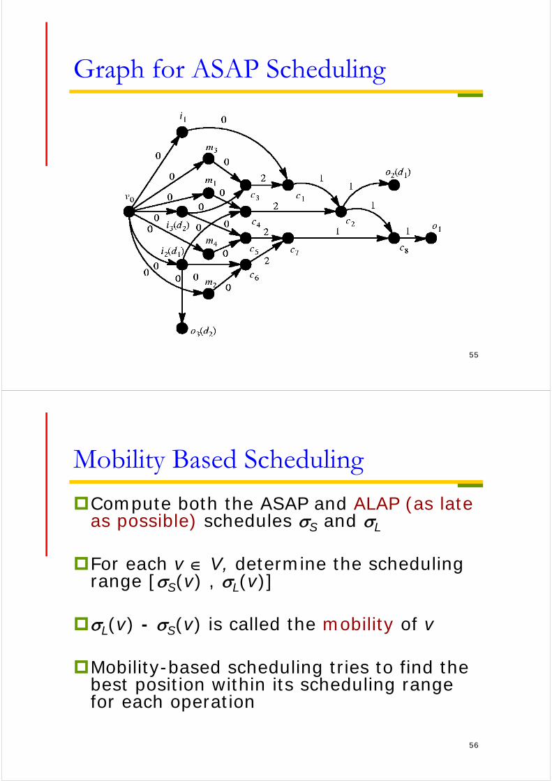
Graph for ASAP Scheduling
56
Mobility Based Scheduling
Compute both the ASAP and ALAP (as late as possible) schedules S and L
For each v V, determine the scheduling range [S(v) , L(v)]
L(v) - S(v) is called the mobility of v
Mobility-based scheduling tries to find the best position within its scheduling range for each operation

57
Simple Mobility Based Scheduling
A partial schedule assigns a scheduling range to each vV,
Finding a schedule can be seen as the generation of a sequence of partial schedules
58
List Scheduling
A resource-constrained scheduling method Start at time zero and increase time until all
operations have been scheduledConsider the precedence constraint
The ready list Lt contains all operations that can start their execution at time t or later
If more operations are ready than there are resources available, use some priority function to choose, e.g. the longest-path to the output node critical-path list scheduling
59
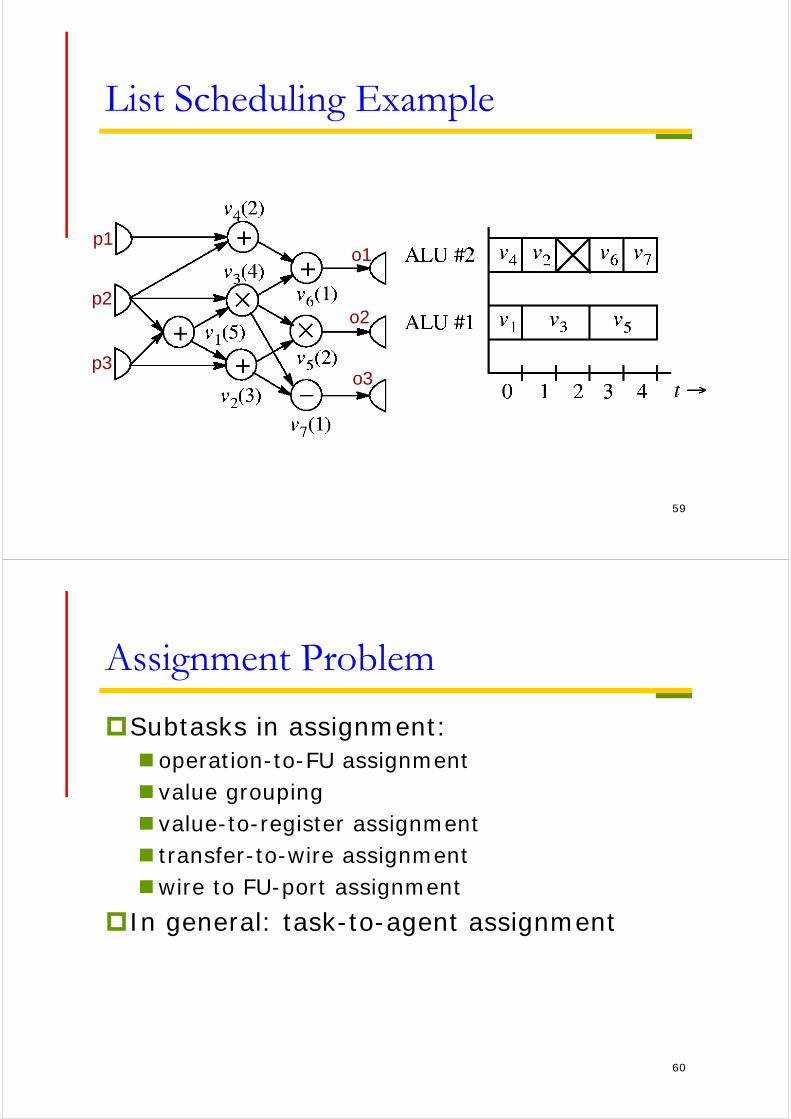
List Scheduling Example
p1
p2
p3o3
o2
o1
60
Assignment Problem
Subtasks in assignment: operation-to-FU assignment value grouping value-to-register assignment transfer-to-wire assignmentwire to FU-port assignment
In general: task-to-agent assignment
61
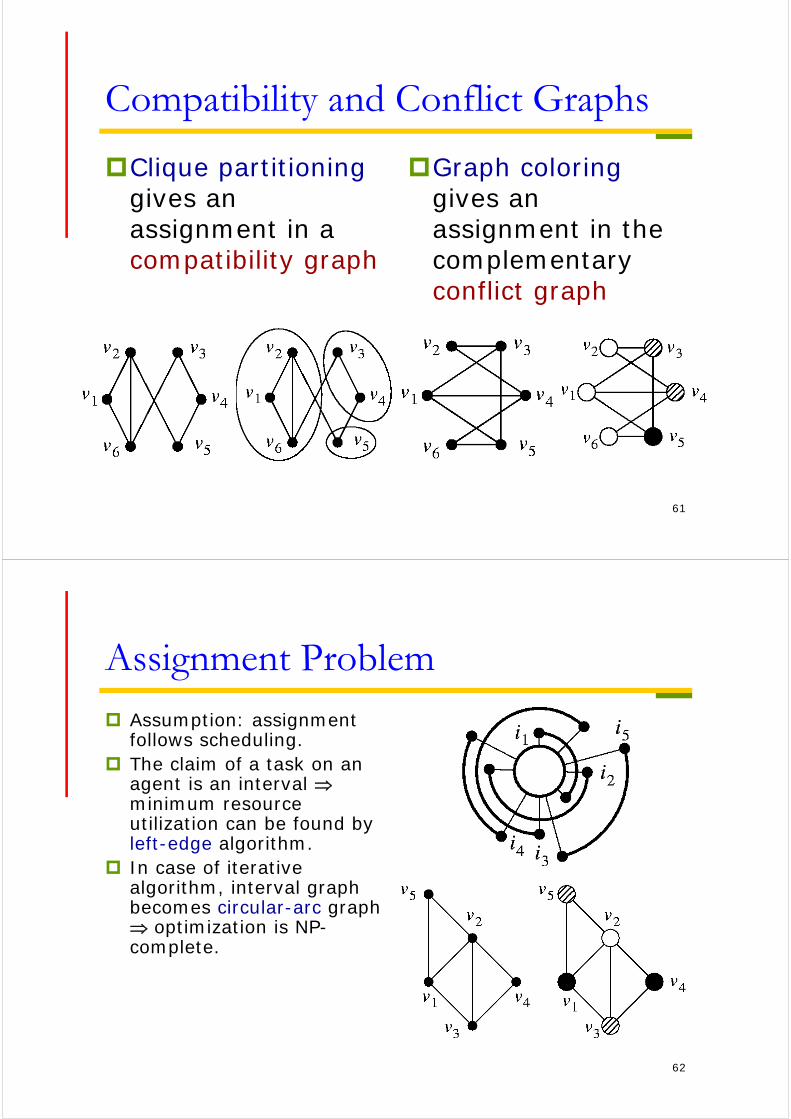
Compatibility and Conflict Graphs
Clique partitioninggives an assignment in a compatibility graph
Graph coloringgives an assignment in the complementary conflict graph
62
Assignment Problem Assumption: assignment
follows scheduling. The claim of a task on an
agent is an interval minimum resource utilization can be found by left-edge algorithm.
In case of iterative algorithm, interval graph becomes circular-arc graph optimization is NP-complete.

63
Tseng and Sieworek’s Algorithm
64
Clique-Partitioning Example

65
Example of Behavior Optimization
Behavior Optimization of Arithmetic Circuit (BOA)
66
Effectiveness of BOASynopsys example


