
Internal Model Design for
Power Electronic Controllers
By
Randupama Tharangani Gunasekara
A thesis submitted to the Faculty of Graduate Studies of
The University of Manitoba
in partial fulfilment of the requirements for the degree of
Master of Science
Department of Electrical and Computer Engineering
University of Manitoba
Winnipeg, Canada
© Copyright 2014 by Randupama T. Gunasekara

Abstract
This thesis deals with the problem of control system design for power electronic control-
lers when high performance is desired despite unaccounted for internal and external con-
ditions. Factors such as parameter variations, operating condition changes, and filtering
and measurements delays, may adversely impact the performance of a circuit whose con-
troller design is not immune to external and internal disturbances. The thesis explores the
method of internal model design as a viable approach for designing controllers with supe-
rior performance despite system variations.
Following a presentation of the theoretical background of the internal model design,
the thesis considers two examples of state variable models, improving the stability of a
voltage source converter and speed control of an induction motor. Conclusions show the
new control system is more stable and offers better controllability despite unexpected
system variations, compared to classical control system.

Acknowledgments
This thesis is the outcome of two years of hard work and I might not have made it suc-
cessfully if I had not got the support of some amazing people. It is an honor to express
my gratitude to all of them at this point. First and foremost I would like to convey my
sincere gratitude to my advisor, Professor Shaahin Filizadeh, for his supervision, invalua-
ble advice and encouragement throughout my Master’s program. His constant stimulating
support helped me tremendously to be critical and analytical in every step required to fin-
ish this thesis.
I would like to thank all my lecturers for their support, help, and valuable advice. I
am glad to thank my examination committee for accepting to review my thesis. I would
also like to thank Prof. Filizadeh and the University of Manitoba for providing me with
financial support and making it possible for me to complete this thesis.
I would also like to express my heartfelt gratitude to my parents and siblings who
gave me support and strength throughout my life and made me able to pursue my goals.
Last but not the least; I would like to thank all those who have offered a hand to the com-
pletion of this research directly or indirectly. Your contribution is appreciated and always
remembered.
Randupama T. Gunasekara

Dedication
To my loving parents

Contents
Contents ......................................................................................................... v
List of Tables ............................................................................................... viii
List of Figures ............................................................................................... ix
List of Symbols ............................................................................................ xiv
List of Abbreviations ................................................................................... xv
1. Introduction 1
1.1 Power Electronic Controllers ................................................................ 1
1.2 Semiconductor Devices and Their Applications ................................... 2
1.2.1 Uncontrolled semiconductor devices .......................................... 2
1.2.2 Semi-controlled semiconductor devices ...................................... 3
1.2.3 Fully-controlled semiconductor devices ..................................... 4
1.3 Motivation .............................................................................................. 6
1.4 Objectives of the research ..................................................................... 7
1.5 Software tools ........................................................................................ 8
1.6 Thesis outline ......................................................................................... 8
2. Background and Literature Review 10
2.1 Introduction ......................................................................................... 10
2.2 Internal Model Design Structure ........................................................ 13
3. The Method of Internal Model Design 18
3.1 Main Controlling Strategies ......................................................................... 18

3.2 Internal model design ............................................................................ 20
3.3 Internal model design examples ........................................................... 22
3.3.1 Example 1 ................................................................................... 22
3.3.2 Example 2 ................................................................................... 30
4. Modified Control System for Active and Reactive Power Control of a
Voltage-Source Converter 45
4.1 Voltage Source Converter ...................................................................... 45
4.2 Introduction of the application .............................................................. 46
4.3 Mathematical Modeling of the Basic Decoupled Control System ........ 48
4.4 Mathematical modeling of the internal model design.......................... 59
4.4.1 Method 1: (control system with an internal model design) ....... 60
4.4.2 Method 2: (control system with the state observer) .................. 63
4.5 Simulation results ................................................................................. 68
4.5.1 System current behavior after adding a filter to the system .... 70
4.5.2 System current behavior after changing the inductance of the
system by 1 percent without adding the filter.................................... 74
4.5.3 System current behavior after changing the inductance of the
system by 5 percent without adding the filter.................................... 77
4.5.4 System current behavior after changing the inductance of the
system by 10 percent without adding the filter.................................. 79
4.5.5 System current behavior after changing the inductance of the
system by 10 percent with the filter ................................................... 81
5. Vector Controlled Induction Motor Drives 84
5.1 Induction machine model ...................................................................... 85
5.2 Vector control methodology ................................................................... 88
5.3 Implementation of the vector control strategy ..................................... 90
5.3 Addition of the internal model to the indirect vector control of the
induction machine ....................................................................................... 95

5.4 Controller response with and without internal model to internal
parameter change of the machine ............................................................... 97
6. Conclusions, Contributions and Future Work 100
6.1 Conclusions and Contributions ........................................................... 100
6.2 Future Work ......................................................................................... 103
7. Reference………………………………………………………………………107

List of Tables
Table 4-1 - Voltage source converter system parameters ................................................. 57
Table 5-1 - Induction motor Drive system parameters ..................................................... 93

List of Figures
Figure 1-1 – Diode (a) circuit symbol, (b) v-i characteristics, (c) ideal v-i characteristics 3
Figure 1-2 – Thyristor (a) Circuit symbol, (b) v-i characteristics ....................................... 4
Figure 1-3 - Block diagram of a power electronic controller ............................................. 5
Figure 2-1 - Classical feedback structure.......................................................................... 13
Figure 2-2 - Modified Classical feedback structure .......................................................... 14
Figure 2-3 - Simplified version of Figure 2.2 ................................................................... 14
Figure 2-4 - Simplified version of Figure 2-3 ................................................................... 15
Figure 3-1 - Block diagram of the modified control system ............................................. 22
Figure 3-2 - Classical control system, designed for example 1 ........................................ 23
Figure 3-3 - Step reference input given to the system ...................................................... 23
Figure 3-4 - Modified control system, designed for example 1 ........................................ 24
Figure 3-5 - Modified control system, designed for example 1 with the state space
observer ............................................................................................................................. 24
Figure 3-6 – Output of the three control strategies designed for example 1 ..................... 29
Figure 3-7 - Output of example 1 when the reference is changed to 10 ........................... 29
Figure 3-8 - Classical control system designed for Example 2 (a) controlled input 1 to the
system (b) controlled input 2 to the system ...................................................................... 31
Figure 3-9 – (a) Reference 1, (b) Reference 2, inputs given to the example 2 ................. 32

Figure 3-10 - Modified control system designed for (a) input 1 (b) input 2, for Example 2
........................................................................................................................................... 33
Figure 3-11 - Modified control systems designed for (a) input 1 (b) input 2, of Example 2
using the state observer ..................................................................................................... 34
Figure 3-12 – (a) Output 1 (y1), (b) Output 2 (y2), of three control strategies designed for
example 2 .......................................................................................................................... 38
Figure 3-13 - Output 1 (y1) of example 2 when the reference is changed to 10 ............... 39
Figure 3-14 - Output 2 (y2) of example 2 when the reference is changed to 10 ............... 39
Figure 3-15 – Random noise given to system given by example 2 .................................. 40
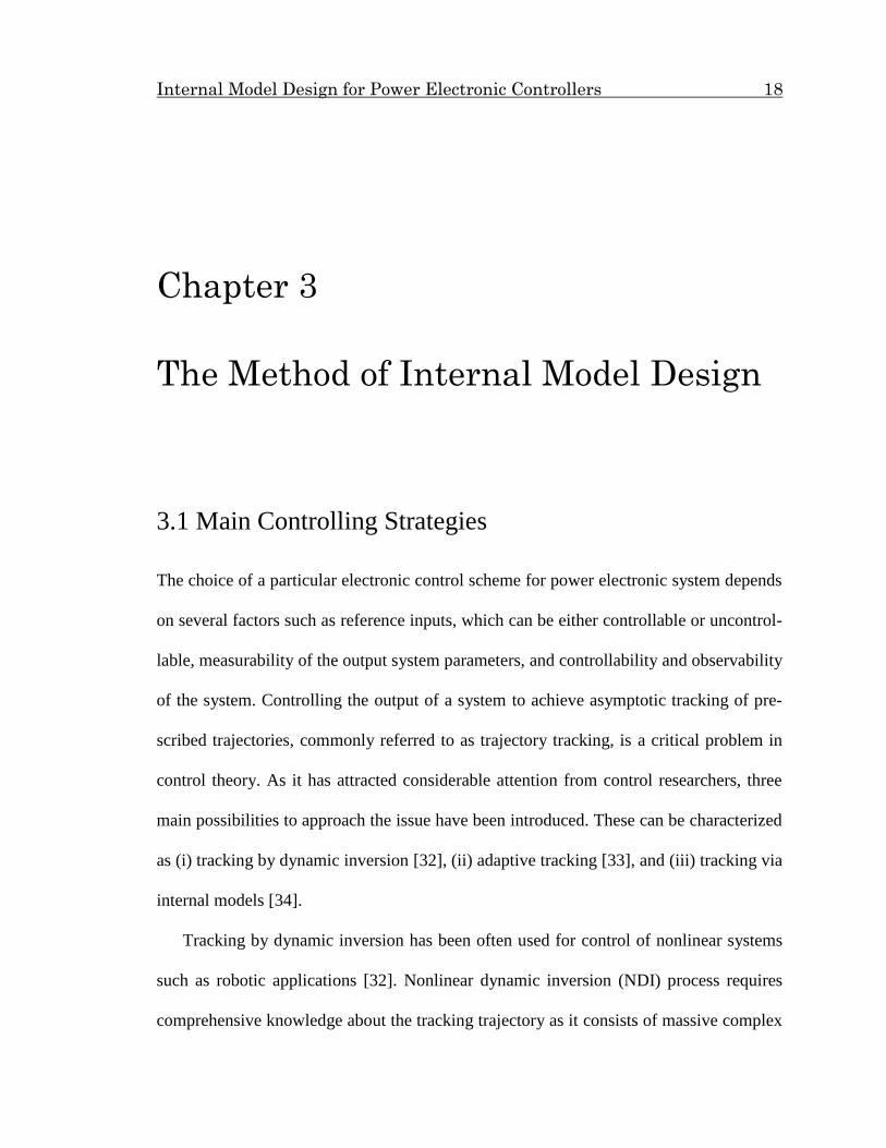
Figure 3-16 – (a) Output 1 (y1), (b) Output 2 (y2), of the three control strategies designed
for example 2 when a random noise is applied ................................................................. 41
Figure 3-17 – (a) Output 1 (y1), (b) Output 2 (y2), of three control strategies designed for
example 2, when the random noise is applied .................................................................. 42
Figure 3-18 – (a) Output 1 (y1), (b) Output 2 (y2), of the three control strategies designed
for of example 2 when a filter is added to the system ..................................................... 43
Figure 4-1- Equivalent circuit diagram of the converter connected to the power system 46
Figure 4-2 - Controlled (a) input 1 (b) input 2, to the system ........................................... 54
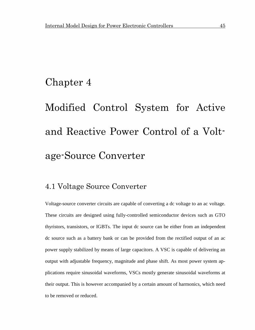
Figure 4-3- Reference input currents (a) Iq_ref, (b) Id_ref , given to the system .................. 55
Figure 4-4 - Representation of the power system equations (a) (4-41) and (b) (4-42) in
block diagrams .................................................................................................................. 56
Figure 4-5- Representation of the power system .............................................................. 56
Figure 4-6 - Classical control system (a) d axis (b) q axis, designed for the power system
........................................................................................................................................... 57

Figure 4-7 – Reference and system currents (a) in q axis, (b) in d axis, of the classical
control system ................................................................................................................... 58
Figure 4-8 - Representation of the classical control system (a) d axis (b) q axis, with
equivalent model of the power system.............................................................................. 59
Figure 4-9 – (a) d axis (b) q axis, modified control systems with internal model designs 61
Figure 4-10 - Reference currents given to the controllers and the system currents (a) in q
axis, (b) in d axis ............................................................................................................... 62
Figure 4-11 - (a) d axis (b) q axis, modified control systems with state observer ............ 66
Figure 4-12 - Reference currents given to the controllers and system currents (a) in q axis,
(b) in d axis ....................................................................................................................... 67
Figure 4-13 - Reference currents and the system currents (a) in q axis, (b) in d axis when
the classical controller and the modified controller (using method 1) are used ............... 68
Figure 4-14 - Reference currents and the system currents (a) in q axis, (b) in d axis when
the classical controller and the modified controller (using method 2) are used ............... 69
Figure 4-15 - Reference currents and the filtered system currents (a) in q axis, (b) in d
axis when the classical controller is used ......................................................................... 71
Figure 4-16 - Reference currents and the filtered system currents (a) in q axis, (b) in d
axis, of the modified controller designed using method 1 ................................................ 72
Figure 4-17 - Reference currents and the filtered system currents (a) in q axis, (b) in d
axis, of the modified controller designed using method 2 ................................................ 73
Figure 4-18 - Reference currents and the system currents (a) in q axis, (b) in d axis when
the classical controller is used (with 1% inductance change and without adding a filter) 74

Figure 4-19 - Reference currents and the system currents (a) in q axis, (b) in d axis, of the
modified controller designed using method 1 (with 1% inductance change and without
adding a filter) ................................................................................................................... 75
Figure 4-20 - Reference currents and the system currents (a) in q axis, (b) in d axis, of the
modified controller designed using method 2 (with 1% inductance change and without
adding the filter) ................................................................................................................ 76
Figure 4-21 - Reference currents and the system currents (a) in q axis, (b) in d axis when
the classical controller is used (with 5% inductance change and without adding the filter)
........................................................................................................................................... 77
Figure 4-22 - Reference currents and the system currents (a) in q axis, (b) in d axis, of the
modified controller designed using method 1 (with 5% inductance change and without
adding the filter) ................................................................................................................ 78
Figure 4-23 - Reference currents and the system currents (a) in q axis, (b) in d axis when
the classical controller is used (with 10% inductance change and without adding the
filter) ................................................................................................................................. 79
Figure 4-24 - Reference currents and the system currents (a) in q axis, (b) in d axis, of the
modified controller designed using method 1 (with 10% inductance change and without
adding a filter) ................................................................................................................... 80
Figure 4-25 - Reference currents and the system currents (a) in q axis, (b) in d axis when
the classical controller is used (with 10% inductance change and after adding a filter) .. 81
Figure 4-26 - Reference currents and the system currents (a) in q axis, (b) in d axis when
the modified controller (using method 1) is used ............................................................. 82
Figure 5-1 – A three phase two pole induction machine .................................................. 85

Figure 5-2 – Reference frame for transformation ............................................................. 87
Figure 5-3 – Torque command generator ......................................................................... 92
Figure 5-4 – Induction vector control schematic diagram ................................................ 92
Figure 5-5 – PSCAD/EMTDC simulation for indirect vector control of induction motor94
Figure 5-6 – Set speed and the machine actual speed ....................................................... 94
Figure 5-7 – Set speed and the actual speed of the machine ............................................ 95

List of Symbols
L - Inductance
C - Capacitance
V - Voltage
R - Resistance
R(t) - Reference
U(t) - Input
Y(t) - Output
E(t) - Error
G(t) - Process
D(t) - Disturbance
x - State vector
x - Estimate of the state x
ξ - Damping ratio
ω - Angular velocity

List of Abbreviations
DC - Direct Current
HVDC - High Voltage Direct Current
AC - Alternating Current
GTO - Gate Turn off Thyristor
BJT - Bipolar Junction Transistor
MOSFET - Metal-Oxide Semiconductor Field-Effect Transistor
IGBT - Insulted gate bipolar transistor
UPS - Uninterruptible Power Supply
SITH - Static Induction Thyristor
MCT - MOS Controlled Thyristor
PSCAD - Power System Computer Aided Design
EMTDC - Electromagnetic Transients including DC
VSC - Voltage Source Converter
PID - Proportional Integral Derivative
NDI - Nonlinear dynamic inversion
IMC - Internal Model Controller
SCR - Silicon Controlled Rectifier
PLL - Phase Locked Loop

Chapter 1
Introduction
1.1 Power Electronic Controllers
One of the main developments that has revolutionized the electrical engineering industry
is the advent of power electronics. Power electronics can be defined as the engineering
study of switching electronic circuits that convert electrical power from one form to an-
other. During the last few decades, power electronics has enjoyed a massive growth in
manufacturing, aerospace [1]-[4], domestic [5], commercial [6]-[8] and military applica-
tions [6], [9]. With this rapid evolution, not only have the reliability and the performance
of power electronic devices increased but also the size and the cost have been reduced.
With these improved features, power electronics has conquered almost every corner of
the electrical engineering industry. Virtually everywhere, the generated power is repro-
cessed through some form of power electronics before it is finally used.
The technology behind almost all the switching power supplies and other applications
such as power converters [10], inverters [11], motor drives, incandescent lamp dimming
[12], heating applications [8] and motor soft starters [13], is power electronics. It pro-

Internal Model Design for Power Electronic Controllers 2
vides solutions from very small mobile phones to huge turbines and trains; the power
range can vary from milliWatts to GigaWatts. This technological advancement has ena-
bled the rise of new applications and appropriate control systems designed for particular
applications to obtain desired performance.
1.2 Semiconductor Devices and Their Applica-
tions
Power semiconductor devices are the core of power electronics [14] and are used in pow-
er electronic circuits for processing of energy and regulating the voltage or current as de-
sired. In power electronics, semiconductor devices are often used as switches where they
are either on or off depending on the output requirement. This is unlike low-power elec-
tronic circuits in which semiconductor devices are typically used in their active operating
region as amplifiers. Semiconductor devices can be classified in to three main categories,
as detailed bellow, based on how much ability they offer to the designer in controlling
their on/off states.
1.2.1 Uncontrolled semiconductor devices
The on and off processes of these devices cannot be controlled and the device attains its
on/off states depending on the surrounding circuit’s behaviour. A diode is a semiconduc-
tor device with uncontrolled characteristics. Figure 1-1 shows the circuit symbol and v-i
characteristics of a diode.

Internal Model Design for Power Electronic Controllers 3
(a) (b) (c)
When the device is in the on state the voltage across the device is very small or
ideally zero at any current and when it is in the off state the current flowing through it is
very small or ideally zero at any voltage.
1.2.2 Semi-controlled semiconductor devices
Semi-controlled semiconductor devices are turned on by an external control circuit and
once they are turned on the off state of the device will depend on the surrounding cir-
cuit’s conditions.
Modern power electronics was initiated with the invention of the thyristor, which is a
semi-controlled semi-conductor device. Since then it has been widely applied in a large
number of electrical engineering applications, such as power supplies [14], [15], static
Var compensators [16], [17], chopper-fed dc drives, HVDC conversion [18], ac machine
drives [19], heating control [20], [21], lighting and welding control and solid state circuit
breakers [22].
Id Anode
Cathode
Figure 1-1 – Diode (a) circuit symbol, (b) v-i characteristics, (c) ideal v-i characteristics
Id
Vd
On
Off
--
Id
Vp – Forward
voltage drop
--
VB – Reverse breakdown
Voltage
Vd

Internal Model Design for Power Electronic Controllers 4
Thyristors have a rapid turn on when a gate signal is applied to trigger the device. For
a proper turn-on the gate signal must meet a minimum current requirement over a certain
length of time. Figure 1-2 shows the circuit symbol and the v-i characteristics of a thyris-
tors.
(a) (b)
Furthermore thyristors require a certain amount of time to obtain forward blocking
capability following a turn-off. If this time is not provided to the thyristor, and the volt-
age across the device is forward biased, it will start conducting even without a gate pulse.
This phenomenon is called commutation failure and is to be avoided in normal operation.
1.2.3 Fully-controlled semiconductor devices
Fully controlled semiconductor devices have the capability of controlling both on and off
states. These devices differ from each other in many ways such as switching frequency,
gate requirements, capability of blocking the reverse voltage, and available power ratings.
Some of the fully controlled semiconductor devices are gate turn off thyristors (GTO)
[23], bipolar junction transistors (BJT), power MOSFETs, insulted gate bipolar transis-
On
Off
It
Vt Without
gate pulse
Gate pulse applied
It Anode
Cathode
Gate
--
--
Figure 1-2 – Thyristor (a) Circuit symbol, (b) v-i characteristics

Internal Model Design for Power Electronic Controllers 5
tors (IGBT), silicon induction thyristors (SITH) and MOS controlled thyristors (MCT).
These semiconductor devices are used in a variety of power electronic applications as de-
tailed bellow.
GTOs are mainly used in high-power applications such as ac machine drives, uninter-
rupted power systems, photovoltaic and fuel cell inverters and static Var compensators
[24]. BJTs are mostly used in voltage-fed choppers and inverters with frequencies from
10 to 15 kilo-Hertz. IGBTs are used in medium power applications such as relays, power
supplies and drivers for solenoids, contactors, dc and ac motor drives and UPS systems.
Advancements in power electronic devices have created a remarkable impact in the
development of modern converters. With this trend power converters have become in-
creasingly capable of providing reliable power with less loss. Power electronic converters
need proper controllers to regulate their operation to obtain desired output when the input
to the system or the operating conditions of the system is changed.
The following figure shows a block diagram of a generic power electronic system.
As shown in the above figure, the input provided to the high-power system has been
regulated using a power electronic converter under the guidance of a feedback control
system to obtain the desired output.
power electronic
converter
ac or dc
input
voltage or
current
power system/
electric machine
drive/load
ac or dc
output
voltage or
current
output
control process
Figure 1-3 - Block diagram of a power electronic controller

Internal Model Design for Power Electronic Controllers 6
To obtain the desired performance of these applications, power electronic converters
need to be properly controlled. The performance of converters largely relies on the effec-
tiveness of the associated controllers; therefore, it is important to apply an appropriate
control system to the converter to obtain desired output.
To design an effective control system it is essential to have proper knowledge about
the dynamics of the entire system and controlling methodologies. In this research, the
control process of a voltage-source converter (VSC) has been considered. A voltage-
source converter is a popular type of power-electronic converter used in conversion be-
tween ac and dc. There are different methods that can be used to control this type of con-
verters. Direct control and decoupled control are two methods that are practiced com-
monly. In this research a decoupled control strategy has been used (as discussed in detail
in Chapter 3). Furthermore a novel controller consisting of an internal model design to
improve the controller performance of the voltage source converter is presented.
1.3 Motivation
Control systems are often designed with the assumptions of linearity and time invariance,
as these assumptions lower the burden and complexity of the design process. However, in
reality, endogenous conditions such as system parameter changes and exogenous condi-
tions, such as undesired disturbances affecting the plant behaviour and the time delays of
the feedback parameters, may result in control systems providing unexpected results. In
this research, to overcome these effects, the existing control system of a VSC to control
power transfer and vector control system of an induction machine to control its speed

Internal Model Design for Power Electronic Controllers 7
have been modified using an internal model design (which is a predictive loop). The new
control system offers better controllability even in the presence of unexpected situations.
1.4 Objectives of the research
The main objective of this research is to develop advanced decoupled control systems for
VSCs using internal model design techniques. The examples shown include internal
model design for a VSC and a control system to regulate the speed of an induction motor.
These control systems allow the system output to follow a reference time-variant input
even when un-modeled dynamics are considered.
To carry out this task, several steps are required.
i. Identification of the endogenous and exogenous factors that affect control systems
of a power electronic application;
ii. Study the behaviour of the internal model designs, and carry out few simple ex-
amples;
iii. Check the performance of the modified control systems under different scenarios;
iv. Look for alternative methods that can provide expected results under different cir-
cumstances;
v. Design of a modified decoupled controller with an internal model for a voltage
source converter connected to a power system;
vi. Design of a modified indirect vector controller with an internal model for an in-
duction machine to regulate the speed;

Internal Model Design for Power Electronic Controllers 8
vii. Implementation of the control system and the power system model in simulation
software;
viii. Tuning controllers to achieve expected output;
ix. Check the performance by testing the simulation case under different scenarios;
x. Compare the results with the existing control system.
1.5 Software tools
The software program used for simulation of the system model in this thesis is the
PSCAD/EMTDC software. PSCAD stands for Power System CAD and EMTDC stands
for Electromagnetic Transients including DC. PSCAD/EMTDC is one of the most popu-
lar electromagnetic transient simulation software packages and it is developed at the
Manitoba HVDC Research Center. This software tool is being used in high power indus-
trial applications such as power system planning, operation, commissioning and research.
EMTDC is the computational engine of the simulator and numerically solves the dif-
ferential equations of the electrical power system network. PSCAD provides the graph-
ical user interface. Running simulation cases, analysing results, schematically construct-
ing circuits and presenting the data in an integrated graphical environment are features of
this simulation tool
1.6 Thesis outline
Chapter 2 of the thesis presents a literature survey, which describes the status of the sub-
ject presently available in the literature.
Internal Model Design for Power Electronic Controllers 9
Chapter 3 describes different control strategies used for tracking a reference given to
the controller. Furthermore, Chapter 3 illustrates how to design a compensator that pro-
vides asymptotic tracking with zero steady state error. It also includes a discussion of de-
signing internal models for a number of simple examples including several alternative
methods.
Chapter 4 describes a voltage-source converter and its power system applications,
which will be controlled by the new controller. Furthermore mathematical modeling of
the voltage source converter is described. How to design the decoupled controller and the
modified controller with the internal model design are also described in this chapter. Ad-
ditionally system models implemented in the PSCAD/EMTDC software, which show the
performance under different circumstances such as delays in the feedback system and cir-
cuit parameter variations are presented.
Chapter 5 describes the design of a control system to regulate the speed of an induc-
tion machine. A dynamic model of an induction motor is reviewed and equations for the
current, voltage, and torque in a rotting dq0 frame are derived. An indirect vector control
strategy is designed for the induction machine to track a set machine speed. Then an in-
ternal model controller is added to the existing control system and its performance is
evaluated. As the rotor resistance of an induction machine can change over time and dur-
ing operation, controller performance is checked with and without an internal model de-
sign to observe how it responds to system parameter changes.
Chapter 6 describes the conclusions and it presents future directions along which fur-
ther research can be conducted.

Internal Model Design for Power Electronic Controllers 10
Chapter 2
Background and Literature Review
2.1 Introduction
A control system is the linking mechanism of components forming a power system con-
figuration that provides a desired output in response to a reference input. Effective con-
trol requires understanding and modeling of the system to be controlled. Originally, con-
trol theory was limited to enhance the performance and stability of single-input single-
output (SISO) systems; additionally time-variant plant conditions were often not consid-
ered. These simplifying assumptions were often applied even when the actual system did
not fully manifest such properties. With the increasingly strict operating conditions of
modern power systems control systems had to be designed to control complex power ap-

Internal Model Design for Power Electronic Controllers 11
plications, which include uncertainties in the system. These control systems should be ro-
bust and provide the expected output not only under predefined system conditions but al-
so under unexpected system conditions (up to certain limits). These uncertainties depend
on different operating conditions of the system and its applications. If it is a power sys-
tem application, system parameter changes may include variations of inductor, resistor or
capacitance values due to aging of parameters or temperature. Fault conditions or addi-
tion of system components such as electric machinery, converters and distributed genera-
tors can also introduce uncertainties to the power systems. The adverse impacts of these
unexpected situations can be partly eliminated by designing the system with large safety
margins, which will adversely affect their cost, or they can be tackled through proper
control systems.
One major problem that may cause instability or otherwise undesirable performance
of a feedback control system is time delay [25]. When the delay is small conventional
controllers (such as proportional-integral-derivative (PID) controllers) could be used but
with the increase of the delay, the process delivers poor performance as it requires signif-
icant detuning to maintain the stability of the control system. Therefore, to overcome
these problem researchers have come up with several alternative control methods [26].
For proper control of a power system, measurements should be fed to the control sys-
tem. To carry out this task variables must be properly measured. However, system varia-
bles may not always be properly measured due to system uncertainties, or it may not be
possible to directly measured them; to overcome this issue, researchers have developed
methodologies to observe the states of a power system. These state observers are used to
Internal Model Design for Power Electronic Controllers 12
enhance the performance of the existing control systems by providing reliable estimations
of crucial variables without directly measuring them.
Kalman filtering is one approach used to estimate the unknown variables of a system
more precisely than the readings based on a single measurement [27]. It uses a series of
measurements of the states of the system over time to provide the estimate. More im-
portantly it provides better performance compared to ordinary feedback controllers under
noisy system conditions. The Smith predictor algorithm is another type of algorithm that
is used to design controllers where system variables need to be observed [28]. It provides
better results compared to ordinary feedback controllers for systems with pure time de-
lays. These state observer methodologies control the system using the predicted output
rather than the actual output. Therefore the implementation is dependent mostly on the
accuracy of the prediction. Most of the controllers deliver optimal responses in absence
of predicted model uncertainties.
Internal model controller (IMC) design is another methodology to observe the states
of a power system for the purpose of its control. The IMC structure was initially devel-
oped for chemical process applications. It became popular as a robust control method for
other control engineering practice, such as disk drive servomechanisms [29] and it is
widely used in robotic applications where trajectory tracking is involved [30]. Several in-
ternal model designs were developed for disturbance compensation in different applica-
tions [31]. Internal model designs have been modified to perform different tasks. For in-
stance some applications require disturbance rejection internal designs whereas other ap-
plications concentrate more on reducing the effect of time delays in systems. Though

Internal Model Design for Power Electronic Controllers 13
there have been plenty of IMC techniques developed, still certain enhancements and ad-
vances are possible to improve the performance of IMC based controllers.
2.2 Internal Model Design Structure
Figure 2-1 illustrates the configuration of a classical feedback structure. The difference
between the reference value and the output (error E(s)) is sent through the controller
(C(s)). Then the controlled input U(s) is fed to the process. Finally the output is compared
with the reference and the process continues. The disturbance D(s) denotes inputs to the
systems that are not controllable by the operator; for example these may include loading
conditions that are imposed externall and to which the system has to react.
Internal model designs can be implemented by modifying the classical feedback con-
trol system. Figure 2-2 illustrates the modified version of the classical control system,
which incorporates an internal model.
reference
R(s)
error
E(s)
Y(s)
output
input
U(s)
controller
C(s)
+
-
+
+
G(s)
process
disturbance
D(s)
Figure 2-1 - Classical feedback structure

Internal Model Design for Power Electronic Controllers 14
As per Figure 2-2, it can be seen that a predictive process model of the actual process
is added and subtracted to/from the classical control structure of Figure 2-1. The control-
ler (C(s)) and the predictive process (Gm(s)) (shown together inside the dashed box) can
be represented as a new controller (Cn(s)) as shown in Figure 2-3.
process
G(s)
+
Y(s)
+
D(s)
+
-
+ -
R(s) U(s) new controller
Cn(s)
predictive
process
Gm(s)
E(s)
E(s)
Y(s)
+
D(s)
+
- +
controller
C(s)
predictive
process
Gm(s)
U(s) process
G(s)
predictive
process
Gm(s) -
+
+
R(s)
Figure 2-2 - Modified Classical feedback structure
Figure 2-3 - Simplified version of Figure 2.2

Internal Model Design for Power Electronic Controllers 15
Figure 2-4 shows an equivalent arrangement, in which the predictive process is
moved in parallel with the controller Cn(s).
As per Figure 2-4, the new controller Cn(s) and the internal model are encircled by the
dashed box; this illustrates that the predictive model of the process is fed back to the new
controller as an internal loop and provide the controlled input to the process.
From Figure 2-1, the following equations can be obtained.
(s) (s) = (s)E C U (2.1)
Similarly, the following equations are obtained from Figure 2-4,
m n( (s) (s) (s)) (s) = (s)E U G C U (2.2)
Using (2.1) and (2.2) following Equations can be derived:
n
m
(s)(s) =
1 (s) (s)
CC
G C (2.3)
n
m n
(s)(s) =
1 (s) (s)
CC
G C (2.4)
Figure 2-4 - Simplified version of Figure 2-3
E(s)
Y(s)
+
D(s)
+
+
+ new controller
Cn(s)
predictive
Process
Gm(s)
U(s) process
G(s) + -
R(s)
Internal Model Design for Power Electronic Controllers 16
According to equation (2.4) it can be seen that the internal model control system
shown in Figure 2-4 can be characterized as a control mechanism consisting of the new
controller Cn(s) and a predictive model Gm(s) of the plant. The internal model controls the
input provided to the process by controlling the difference between the output of the pro-
cess and the reference value. This error can occur due to disturbances or other mismatch-
es of the model.
From Figure 2-4, the output of the system can be expressed as:
(s) = (s) (s) (s)Y U G D (2.5)
Using equation (2.1), Y(s) can be expressed as:
(s) = (s) (s) (s) (s)Y E C G D (2.6)
Error E(s) is:
(s) = (s) (s)E R Y (2.7)
Using equation (2.7), Y(s) can be expressed as:
(s) = ( (s) (s)) (s) (s) (s)Y R Y C G D (2.8)
By rearranging the equation (2.8), Y(s) can be expressed as:
(s) (s) (s)(s) =
1 (s) (s) 1 (s) (s)
G R DY
C G C G
(2.9)
Using equation (2.4) the output of the system can be expressed as follows.
n m n
n m n m
(s) (s) (s) (1 (s) (s)) (s)(s) =
1 (s)( (s) (s)) 1 (s)( (s) (s))
G C R G C DY
C G G C G G
(2.10)
If the plant can be modeled correctly where Gm(s) is equal to G(s) and if the disturb-
ance is absent, from (2.10) the system becomes an open loop one. Based on the stability
of Cn(s) and G(s), closed-loop stability is characterized.
Internal Model Design for Power Electronic Controllers 17
According to (2.4) it can be seen that the closed-loop stability is dependent on the
stability of the new controller Cn(s) and the model of the process G(s). If the process
model and the predictive model are equal and the new controller is the inverse of the pro-
cess 1(s) = (s)nC G the system can be controlled to obtain the expected output from the
system given that the model of the system is stable. Therefore IMC is a useful concept,
which allows an open-loop controller to provide closed-loop performance. Thus the IMC
structure offers better performance to obtain expected results from a process compared to
a classical feedback controller. However, selection or design of a compensator is a criti-
cal task as it can create instability in the presence of disturbances and plant model mis-
matches. Filters are used in power system controllers to make them more robust and to
help in minimizing the discrepancies between the plant and the model. But as a conse-
quence it produces delays in the system and leads to decrease the efficiency of the con-
troller. Therefore designing a controller for a power system has become a critical task.
In this research, a controller has been designed including an internal model design to
control a VSC and an induction machine. This controller is a dynamic compensator that
can be used for set point tracking applications providing expected results.
Internal Model Design for Power Electronic Controllers 18
Chapter 3
The Method of Internal Model Design
3.1 Main Controlling Strategies
The choice of a particular electronic control scheme for power electronic system depends
on several factors such as reference inputs, which can be either controllable or uncontrol-
lable, measurability of the output system parameters, and controllability and observability
of the system. Controlling the output of a system to achieve asymptotic tracking of pre-
scribed trajectories, commonly referred to as trajectory tracking, is a critical problem in
control theory. As it has attracted considerable attention from control researchers, three
main possibilities to approach the issue have been introduced. These can be characterized
as (i) tracking by dynamic inversion [32], (ii) adaptive tracking [33], and (iii) tracking via
internal models [34].
Tracking by dynamic inversion has been often used for control of nonlinear systems
such as robotic applications [32]. Nonlinear dynamic inversion (NDI) process requires
comprehensive knowledge about the tracking trajectory as it consists of massive complex

Internal Model Design for Power Electronic Controllers 19
calculations for computation of the initial conditions and the feedback of the system. In
adaptive tracking, the controller structure consists of a feedback loop and a controller
with an adjustable gain [33]. This method can effectively handle parameter uncertainties,
but the knowledge of the entire trajectory is needed to be used for designing the adapta-
tion algorithm. Therefore these approaches are not well-suited for applications with un-
known trajectories.
Internal model-based tracking, which is used in this research, has the capability of
handling uncertainties simultaneously in the plant parameters as well as in the trajectory
to be followed. Furthermore, time delays, which can occur due to external conditions, can
be compensated by this method for proper functionality of the control system. Filtering of
output parameters, which are extracted from the system to feed to the controller, is an ex-
ternal condition that can cause time delay. Moreover it has been proven that a controller
designed with an internal model is able to secure asymptotic decay to zero of the tracking
error for every possible trajectory and it can perform robustly with respect to parameter
uncertainties of the system [35]. Therefore internal model control design is a very prom-
ising method that can be used for many power system applications. However the control-
lers designed using IMC concept can be costly due to the additional sensors that are
needed to measure the system parameters for internal loop feedback, and they may also
slow down the controller process. In this chapter the fundamentals of the internal model-
based design method are presented.

Internal Model Design for Power Electronic Controllers 20
3.2 Internal model design
A controller can face a great deal of unexpected environment changes of its applications
in real time implementation. These unpredicted phenomena could occur due to endoge-
nous conditions such as system parameter variations, or exogenous conditions, such as
additional undesired inputs affecting the plant behaviour and the time delays of the feed-
back parameters.
In this section, the design of a compensator that provides asymptotic tracking of a
reference input with zero steady state error is considered. Reference inputs considered in-
clude steps, ramps, sinusoids, etc. If the plant can be modeled as a linear, finite-
dimensional, time-invariant system, the controller can be developed as follows. Suppose
that the model of the plant is a set of first-order linear differential equations, written in the
form.
= ux A x + B (3.1)
=y C x (3.2)
where x is the state vector, u is the input and y is the output.
Let a reference input r to be generated by a linear system be of the form,
= r r rx A x (3.3)
= r rr d x (3.4)
When the input is a step response, then:
= 0rx (3.5)
= rr x (3.6)

Internal Model Design for Power Electronic Controllers 21
t
1
0
( ) = - ( ) - ( )u t K e d t 2K x
Or equivalently,
= 0r (3.7)
The tracking error (e(t)) can be defined as follows,
=e y - r (3.8)
Taking the time derivative of the error yields:
=e y (3.9)
Taking the time derivative of (3.2) yields:
=y Cx (3.10)
Let two intermediate variables v and ω be defined as follows:
=v x (3.11)
= u (3.12)
From (3.11) and (3.12) the following state-space representation can be obtained.
0 0= +
0
e e
C
v A v B (3.13)
If (3.13) is controllable, feedback can be written in the following form so that the
above equation will be stable.
= 1- K e 2
K v (3.14)
where K1 and K2 are constants
Stability of the equation (3.13) implies the tracking error stability; therefore, the ob-
jective of asymptotic tracking with zero steady state error can be achieved. The control
input can be found using above equation (3.14) as shown below,
(3.15)

Internal Model Design for Power Electronic Controllers 22
The corresponding block diagram of the developed scheme is shown in Figure 3-1.
+K1
1
sT
+
-
Transfer
Function
C
K2
Reference- Output (y)Input (U)Error (E)
x
Figure 3-1 - Block diagram of the modified control system
As per the diagram, the error (E) which is the difference between the reference and
the output, is multiplied by a constant and sent through an integrator. After that, the result
is subtracted from the state parameter generated by the system and then fed to the system
as the real input. The dashed box represents the controller including the internal model.
3.3 Internal model design examples
3.3.1 Example 1
In this section, a first-order system is used to demonstrate the performance of the internal
model concept from Section 3.2. First a classical controller is designed and then it is
modified using the internal model concept.
Consider the following first-order single-input, single-output system.
= 5 + 2ux x (3.16)
= 2y x (3.17)
In Laplace domain,
s = 5 + 2ux x (3.18)

Internal Model Design for Power Electronic Controllers 23
and the system transfer function can be written as follows.
2 =
s - 5
ux (3.19)
To compare the performance of the modified controller and the classical system three
system models have been built with different controlling strategies.
3.3.1.1 Case 1 (Classical control system)
Case 1
Output
C
Transfer
Function of
(3.19)
+
-Reference
I
Px y
Figure 3-2 - Classical control system, designed for example 1
Figure 3-2 shows a classical control system built to control the output of the system. As
shown a simple proportional-integral (PI) controller has been used to control the error be-
tween the reference and the output. The PI controller has been well tuned to follow the
reference. The reference is varied as shown in the Figure 3-3.
0.0 2.5 5.0 7.5 10.0 12.5 15.0 17.5 20.0 -6.0
-4.0
-2.0
0.0
2.0
4.0
6.0
8.0
10.0
12.0
Reference
Time (sec)
Refe
rence v
alu
e o
f th
e s
yste
m
Figure 3-3 - Step reference input given to the system

Internal Model Design for Power Electronic Controllers 24
3.3.1.2 Case 2 (control system with an internal model)
+
-
1
sT1000
+
-
C
Transfer
Function of
(3.19)Reference Case 2
Output
x y
Figure 3-4 - Modified control system, designed for example 1
Figure 3-4 shows the control system built with an internal model design. The integrator is
well tuned, output to follow the reference shown by Figure 3-3 and obtain better perfor-
mance compared to classical control system.
3.3.1.3 Case 3 (control system with an internal model and the observer)
2+-
1000 1
sT+
-
4.92
+
Transfer
Function
Transfer
Function
Case 3
OutputReference
+
x y
Figure 3-5 - Modified control system, designed for example 1 with the state space observer
The configuration shown in Figure 3-5 has been designed similar to case 2 with a modi-
fied state feedback generated using a state observer. The state observer is shown within
the dashed box in Figure 3-5.

Internal Model Design for Power Electronic Controllers 25
3.3.1.3.1 Controllability and observability
One of the key questions that arises while developing a state variable compensator is
whether the system is controllable. This has to do with whether the poles of a closed-loop
system can be arbitrary placed in the complex plane (the poles of a closed loop system
are equivalent to the eigen-values of the system matrix in state variable format). The con-
cept of controllability and observability was heavily investigated by Kalman in 1960
[36], [37].
Consider a system given as follows.
ux = Ax + B (3.20)
= y Cx (3.21)
The controllability can be determined as follows. If the matrix A is an n x n matrix
and if it is a multi-input system, matrix B can be an n x m matrix where m is the number
of inputs to the system. For a single input, single output system the controllability matrix
is defined as follow in terms of A and B,
2 n-1
c P = B AB A B ... A B (3.22)
If cP is an n x n matrix and the determinant is non-zero, the system is controllable [38].
E. g. 2 0
= 2 3
A
1 =
0
B = 0 1C
-2
= 2
AB
Therefore c
1 -2=
0 2
P

Internal Model Design for Power Electronic Controllers 26
0 1 0
= 0 0 1
- - -
A
X Y Z
= 1 0 0C
and the determinant of the Pc matrix is 2 therefore the system is controllable.
Consider the single input, single output system given by,
= + ux Ax B (3.23)
= y Cx (3.24)
where C is a 1 x n row vector and x is an n x 1 column vector. For the above system, the
observability matrix can be written as follows.
o
-1
=
n
C
CA
.P
.
.
CA
Po is an n x n matrix.
For and
= 0 1 0CA and 2 = 1 0 0CA thus it is observed that:
o
1 0 0
= 0 1 0
0 0 1
P
where the determinant of Po is 1. Therefore the system is observable.

Internal Model Design for Power Electronic Controllers 27
3.3.1.3.2 State observer design
In designing a state observer process, first assume that all the states are available for the
feedback. According to Luenberger [39], a full state observer for the system,
= + ux Ax B (3.25)
= y Cx (3.26)
is given as follows.
= + + ( - )u yx Ax B L Cx (3.27)
where x denotes the estimate of the state x and the matrix L is the observer gain matrix,
which will be determined as part of the observer design. In this case the observer pro-
vides an estimate ( x ) so that it will reach x asymptotically. The estimation error can be
written as follows.
( ) = ( ) - ( )t t te x x (3.28)
To achieve the goal of the observer, the L matrix is designed so that the tracking error
will be asymptotically stable as the error 𝒆(𝑡) tends to zero.
Taking the time derivative of the error shown by equation (3.28),
= - e x x (3.29)
By combining equations (3.27) and (3.29)
= + - - - ( - )u u ye Ax B Ax B L Cx (3.30)
( ) ( ) ( )t t e A LC e (3.31)
If the characteristic equation det (λ - ( - )) = 0I A LC has negative roots, then for any ini-

Internal Model Design for Power Electronic Controllers 28
tial tracking error e(t0), the e(t) will tend to zero with time. The L matrix will be calculat-
ed such that the characteristic equation’s (3.31) roots lie on the left half plane.
For a faster response with a lower over-shoot, suppose the characteristic equations
can be written as [40],
nΔ(λ) = (λ + ξ ) (3.32)
where 𝜉 is the damping ratio and 𝜔𝑛 is the angular velocity.
According to example 1 data (Section 3.3.1),
A = 5, C = 2,
det (λ - ( - ) = 0)I A LC (3.33)
By substituting the values in equation (3.33),
λ - (5 - 2 ) = 0L
λ - 5 + 2 = 0L (3.34)
Let 𝜔𝑛 is 6 and 𝜉 to be 0.8 for minimal overshoot [40], using equation (3.34),
L = 4.9
Therefore the observer equation is,
= 5 + 2 + 4.9 ( - 2 )u yx x x (3.35)
The configuration shown in Figure 3-5 has been designed with a modified controller
where the state estimator is designed using above calculated values.

Internal Model Design for Power Electronic Controllers 29
3.3.1.4 Simulation results for Example-1
For the system defined in example 1, a varying step reference was given as shown in Fig-
ure 3-3. The following results were observed for all the 3 cases defined above.
0.0 2.5 5.0 7.5 10.0 12.5 15.0 17.5 20.0 -6.0
-4.0
-2.0
0.0
2.0
4.0
6.0
8.0
10.0
12.0
Case3
Reference
Case2
Case1
Time (sec)
Outp
ut
valu
e o
f th
e s
yste
m
Figure 3-6 – Output of the three control strategies designed for example 1
Figure 3-6 illustrates how each control system behaves with time when the same ref-
erence input is given to the system. According to the above graph, it can be seen that eve-
ry case has generally followed the reference value but in slightly different ways. The
graph shown in Figure 3-7 gives a closer view of the behaviour of three cases during the
transient period.
6.50 7.00 7.50 8.00 8.50 9.00 9.50 7.0
8.0
9.0
10.0
11.0
12.0
13.0
Case3
Case2
Case1
Reference
Time (sec)
Outp
ut
valu
e o
f th
e s
yste
m
Figure 3-7 - Output of example 1 when the reference is changed to 10

Internal Model Design for Power Electronic Controllers 30
According to this graph, during the transient period, the classical control system (case
1) has a significant overshoot whereas the modified control systems (case 2 and case3)
follow the reference more closely. Furthermore it can be seen that case 2 and case 3
(modified controllers) have produced almost the same output. Hence for this system con-
figuration (given by example 1) the modified control system has performed well com-
pared to the classical system.
3.3.2 Example 2
In this section, a second order system equation is used to check the performance of the in-
ternal model concept discussed in Section 3.2. First a classical controller is designed to
the system and then it is modified using the internal model. Then the case is implemented
in PSCAD/EMTDC software and output results are observed.
The system equation are as follows.
1 1
2 2
2 3 = +
-1 4
u
u
xx
x (3.36)
1
2
1 0 =
0 1y
x
x (3.37)
Taking the Laplace transform of equation (3.36),
1 1 2 1s = 2 +3 + ux x x (3.38)
1 1 2 2s = - + 4 + ux x x (3.39)
Using equation (3.38) and (3.39) transfer functions can be written as,
2 11
3 + =
s - 2
uxx (3.40)

Internal Model Design for Power Electronic Controllers 31
1 22
- + =
s - 4
uxx (3.41)
This case has been implemented in PSCAD/EMTDC software to observe the re-
sponse of the output. To compare the performance of the modified controller and the
classical system, three system models have been built with different controlling strategies
as in Example 1.
3.3.2.1 Case 1 (Classical control system)
I
P
I
P+
-
+
+
3
+
-
+-
Case1 (y1)
Transfer
Function of
(3.40)
Transfer
Function of
(3.41)
Case1 (y1)
Reference1
Case1 (y2)
Reference2 Case1 (y2)
Case1 (y2)
Case1 (y1)
(a)
(b)
Figure 3-8 - Classical control system designed for Example 2 (a) controlled input 1 to the
system (b) controlled input 2 to the system
Figure 3-8 shows a classical control system built to control the input of the system. As
per the Figure 3-8, PI controller has been used and it has been well tuned to follow the
reference which is given as a step sequence as shown in Figure 3-9.

Internal Model Design for Power Electronic Controllers 32
0.0 2.5 5.0 7.5 10.0 12.5 15.0 17.5 20.0 -4.0
-2.0
0.0
2.0
4.0
6.0
8.0
10.0
12.0
Reference1
Time (sec)
Input
(PU
)
(a)
-4.0
-2.0
0.0
2.0
4.0
6.0
8.0
10.0
12.0
Reference2
0.0 2.5 5.0 7.5 10.0 12.5 15.0 17.5 20.0
Time (sec)
Inp
ut
(PU
)
(b)
Figure 3-9 – (a) Reference 1, (b) Reference 2, inputs given to the example 2
The two reference inputs shown in Figure 3-9 are fed to the three control strategies
designed for Example 2 to check the controllers’ responses.

Internal Model Design for Power Electronic Controllers 33
3.3.2.2 Case 2 (control system with an internal model)
+
-
1
sT
+
-
G11=1500+
+Case2 (y1)
Case2 (y1)
Reference1
Case2 (y1) Case2 (y2)
Transfer
Function of
(3.40)
G1
2=
1
G1
3=
3
(a)
+
-
+
-
1
sT
+
- Case2 (y2)
Case2 (y1)
Case2 (y2)
Case2 (y2)
Reference2
Transfer
Function of
(3.41)
G21=1500
G2
2=
1
(b)
Figure 3-10 - Modified control system designed for (a) input 1 (b) input 2, for Example 2
Figure 3-10 shows the modified controller built with an internal model control design.
G11, G12, G13 and G21, G22 are proportional gains of the controller. The integrator is tuned
for the output of the system to follow the reference shown by Figure 3-9 and to obtain
better performance from the above configuration.

Internal Model Design for Power Electronic Controllers 34
(a)
Case3 (y2)
+
-
1
sT
+
-
+
-
-78.5
77.5
+
+
+
+
Case3 (y1)
Case3 (y2)
Reference2
Case3 (y1)
Case3 (y2)
Transfer
Function of
(3.41)U2
U2
Transfer
Function of
(3.54)
G2
2=
1
G12=1500
Case3 (y1)
+
+
+
-
1
sT
+
-
+
+
++
21
2
U1
Case3 (y1)
Reference1
Case3 (Y2)
Case3 (y2)
Case3 (y1)
Transfer
Function of
(3.40)
Transfer
Function of
(3.53)
U1
G11=1500
G1
2=
1
G1
3=
3
(b)
3.3.2.3 Case 3 (control system with an internal model and the observer)
Figure 3-11 - Modified control systems designed for (a) input 1 (b) input 2, of Example 2 using the state
observer
Configuration shown in Figure 3-11 has been designed same as case 2, but the state feed-
back is given using a state observer. G11, G12, G13 and G21, G22 are proportional gains of
the controller.

Internal Model Design for Power Electronic Controllers 35
3.3.2.3.1 Observer Design
To design the observer shown above, the gain matrix and other parameters were calculat-
ed as bellow.
2 3
= -1 4
A 1 0
= 0 1
C 1 0
= 0 1
B
The state observer equation is given bellow.
= + + ( - )u yx Ax B L Cx (3.42)
Where x denotes the estimate of the state x and the L matrix is the observer gain matrix
which will be determined as the part of the observer design.
Estimation error can be written as,
( ) = ( ) - ( )t t te x x (3.43)
Taking the time derivative of error given by equation (3.43),
= - e x x (3.44)
By combining equations (3.42) and (3.44) the following equation can be obtained,
= + - - - ( - )u u ye Ax B Ax B L Cx (3.45)
( ) ( ) ( )t t e A LC e (3.46)
The characteristic equation is:
det (λ - ( - ) ) = 0I A LC (3.47)
For a faster response with a lower over shoot, suppose the characteristic equation of
equation (3.47) can be written as bellow [40],
2 2
n nΔ(λ) = λ + 2ξ λ + (3.48)

Internal Model Design for Power Electronic Controllers 36
where 𝜉 is the damping ratio and 𝜔n is the angular velocity. According to the dimensions
of the system given in this example, the gain matrix (L) can be written as,
1 2
3 4
L L
L L
By substituting the values to the equation (3.47),
1 2
3 4
1 0 2 3 1 0- 0
0 1 -1 4 0 1
L L
L L
1 2
3 4
λ 0 2 3- - = 0
0 λ -1 4
L L
L L
1 2
3 4
2 - 3 - λ 0- = 0
-1- 4 - 0 λ
L L
L L
1 2
3 4
λ - 2 + 3 + = 0
1 + λ - 4 +
L L
L L
1 4 2 3(λ - 2 + )(λ - 4 + ) ( 3)( 1) 0L L L L (3.49)
Assume L2 and L4 to are 1 (for the simplicity of the calculations)
2
1 3 1(λ) = + ( 5) 2 3 8L L L (3.50)
Let 𝜔𝑛 be 10 and select 𝜉 to be 0.8 for minimal overshoot [40], using equation (3.49) and
(3.50), L3 and L1 can be found.
1 5 16L
1 21L
and

Internal Model Design for Power Electronic Controllers 37
3 12 - 3 + 8 = 100L L (3.51)
By substituting the value of L1 to equation (3.51), L3 can be found.
3 = 77.5L
By substituting the values for the observer equation (3.42),
2 3 1 0 21 1 = + + ( - )
-1 4 0 1 77.5 1u y
x x CX (3.52)
Taking the Laplace transform of the above equation,
1 1 2 1 1 1 2 2s = 2 + 3 + + 21 - 21 + - u y yx x x x x
1 2 1 21
+ + 21 + 2 =
s +19
u y y xx (3.53)
And
2 1 2 2 1 1 2 2sx = - + 4 + + 77.5 - 77.5 + - u y yx x x x
2 2 1 12
+ +77.5 -78.5 =
s -3
u y y xx (3.54)
The configuration shown in Figure 3-11 has been designed with a modified controller
where the state estimator is designed using the above calculated values.
3.3.2.4 Simulation results for Example 2
For the system defined in example 2, a varying step reference was given as shown in Fig-
ure 3-9. Following results have been obtained for all the three cases defined above.

Internal Model Design for Power Electronic Controllers 38
0.0 2.5 5.0 7.5 10.0 12.5 15.0 17.5 20.0 -4.0
-2.0
0.0
2.0
4.0
6.0
8.0
10.0
12.0
Reference1
Case2 (y1)
Case1 (y1)
Case3 (y1)
Time (sec)
Input
(PU
)
(a)
-4.0
-2.0
0.0
2.0
4.0
6.0
8.0
10.0
12.0
Reference2
Case2 (y2)
Case1 (y2)
Case3 (y2)
0.0 2.5 5.0 7.5 10.0 12.5 15.0 17.5 20.0
Time (sec)
Inp
ut
(PU
)
(b)
Figure 3-12 – (a) Output 1 (y1), (b) Output 2 (y2), of three control strategies designed for example 2
Figure 3-12 illustrates how each control system behaves with time when the same
reference input is given to the three cases. According to the above graph, it can be seen
that, each case has exactly followed the reference value but in a different manner. The
Figure 3-13 and 3-14 give a closer look of the behaviour of three cases during the transi-
ent period.

Internal Model Design for Power Electronic Controllers 39
8.90 9.00 9.10 9.20 9.30 9.40 9.50 9.25
9.50
9.75
10.00
10.25
10.50
10.75
11.00
11.25
11.50
Reference1
Time (sec)
Ou
tpu
t o
f th
e sy
stem
Case2 (y1)
Case1 (y1)
Case3 (y1)
Figure 3-13 - Output 1 (y1) of example 2 when the reference is changed to 10
6.90 7.00 7.10 7.20 7.30 7.40 7.50 7.60 7.70 9.00
9.25
9.50
9.75
10.00
10.25
10.50
10.75
11.00
11.25
Reference2
Time (sec)
Outp
ut of
the
syst
em
Case2 (y2)
Case1 (y2)
Case3 (y2)
Figure 3-14 - Output 2 (y2) of example 2 when the reference is changed to 10
Figures 3-13 and 3-14 are zoomed in versions of Figure 3-12 and it shows the behav-
iour of the three control systems when the reference value is 10. According to the graph,
during the transient period, it can be seen that the classical control system (case 1) has a
significant overshoot whereas the modified control systems (case 2 and case3) follow the
exact reference. Output 1 (y1) given by Figure 3-7 shows that the settling time of case 1 is
9.32s whereas case 2 and 3 have settled at 9.06s. Therefore modified case has stabilized
0.25s faster than the classical system. Output 2 (y2) shown in Figure 3-7 illustrates that

Internal Model Design for Power Electronic Controllers 40
the settling time of case 1 is 7.32s whereas case 2 and 3 have settled at 7.07s. Therefore
the modified case has stabilized 0.25s faster than the classical system. Furthermore it can
be seen that case 2 and case 3 (modified controllers) have given almost identical outputs.
To observe the controller behaviors, a disturbance was applied to the system de-
scribed in Example 2 and the following results were obtained. Here a random number
generator has been used to give random noise which vary from (-2) to (+2) as shown be-
low.
0.0 2.5 5.0 7.5 10.0 12.5 15.0 17.5 20.0 -1.00
-0.75
-0.50
-0.25
0.00
0.25
0.50
0.75
1.00
Dis
turb
anc
e g
ive
n t
o t
he
sy
ste
m
Time (sec)
Random noise
Figure 3-15 – Random noise given to system given by example 2
Internal Model Design for Power Electronic Controllers 41
0.0 2.5 5.0 7.5 10.0 12.5 15.0 17.5 20.0 -4.0
-2.0
0.0
2.0
4.0
6.0
8.0
10.0
12.0
Reference1
Case1 (y1)
Case2 (y1)
Case3 (y1)
Time (sec)
Outp
ut
of
the
syst
em
(a)
-4.0
-2.0
0.0
2.0
4.0
6.0
8.0
10.0
12.0
Reference2
Case1 (y2)
Case2 (y2)
Case3 (y2)
2.5 5.0 7.5 10.0 12.5 15.0 17.5 20.0 0.0
Time (sec)
Ou
tpu
t o
f th
e sy
stem
(b)
Figure 3-16 – (a) Output 1 (y1), (b) Output 2 (y2), of the three control strategies designed for example 2
when a random noise is applied
Figure 3-16 shows how the random noise has affected the output of the system.

Internal Model Design for Power Electronic Controllers 42
12.450 12.475 12.500 12.525 12.550 12.575 12.600 12.625 12.650 12.675 12.700 8.00
8.50
9.00
9.50
10.00
10.50
Reference1
Case1 (y1)
Case2 (y1)
Case3 (y1)
Ou
tpu
t o
f th
e sy
stem
Time (sec)
3.00
3.50
4.00
4.50
5.00
5.50
6.00
Reference2
Case1 (y2)
Case2 (y2)
Case3 (y2)
12.475 12.500 12.525 12.550 12.575 12.600 12.625 12.650 12.675 12.700
Outp
ut of
the
syst
em
Time (sec)
Figure 3-17 – (a) Output 1 (y1), (b) Output 2 (y2), of three control strategies designed for example 2, when the
random noise is applied
Figure 3-17 is a zoomed in version of Figure 3-16 where the disturbance is applied to
the system and the controllers’ responses are shown. As per the graph it can be seen that
the case 2 and case 3 controllers stabilize faster than the classical case. Therefore it can
be concluded that the modified controller is more fitting for real time power system im-
plementations than the classical method.
For the system given by Example 2, a low pass filter was also applied before feeding
the system. The purpose of this modification was to observe the behaviour of the control
(a)
(b)

Internal Model Design for Power Electronic Controllers 43
-10.0
-5.0
0.0
5.0
10.0
15.0
20.0
Reference2
Case1 (y2)
Case2 (y2)
Case3 (y2)
0.0 2.5 5.0 7.5 10.0 12.5 15.0 17.5 20.0
Outp
ut
of
the
syst
em
Time (sec)
0.0 2.5 5.0 7.5 10.0 12.5 15.0 17.5 20.0 -10.0
-5.0
0.0
5.0
10.0
15.0
Reference1
Case1 (y1)
Case2 (y1)
Case3 (y1)
Outp
ut
of
the
syst
em
Time (sec)
systems when there is a delay in the feedback parameter. This often occurs in real case
scenarios as when the filters are used to extract the system output, there will be a signifi-
cant delay in the feedback system. Therefore PID controllers will be detuned and will not
perform as expected. In this case a 0.05s time delay has given to the outputs of the sys-
tem. This time delay was provided using a 1
1 sT transfer function, where T denotes the
delay time constant.
(a)
(a)
(b)
Figure 3-18 – (a) Output 1 (y1), (b) Output 2 (y2), of the three control strategies designed for of ex-
ample 2 when a filter is added to the system

Internal Model Design for Power Electronic Controllers 44
Examining Figure 3-18 it can be seen that the classical case (case 1) has not per-
formed as expected.
Decoupling refers to the situation where two or more physically coupled systems op-
erate without affecting each other’s performance. In this example the two states of the
system are coupled and each state has an effect on each other, as seen by variations of
one when the other one is given a new command. By using a decoupling control tech-
nique each state can be controlled individually. Close examnitaion of the waveforms in
Figure 3-18 (a) around t =7.5s shows that when the reference 2 is changed (as shown in
Figure 3-18 (b)), the output 1 undergoes a transient. This means with the addition of de-
lay, classical controller has shown lack of decoupling capability.
Comparing to case 1, the other two cases have given the results desired. Therefore it
can again be concluded that the modified controller is more fitting for real time power
system implementations than the classical method.
Internal Model Design for Power Electronic Controllers 45
Chapter 4
Modified Control System for Active
and Reactive Power Control of a Volt-
age-Source Converter
4.1 Voltage Source Converter
Voltage-source converter circuits are capable of converting a dc voltage to an ac voltage.
These circuits are designed using fully-controlled semiconductor devices such as GTO
thyristors, transistors, or IGBTs. The input dc source can be either from an independent
dc source such as a battery bank or can be provided from the rectified output of an ac
power supply stabilized by means of large capacitors. A VSC is capable of delivering an
output with adjustable frequency, magnitude and phase shift. As most power system ap-
plications require sinusoidal waveforms, VSCs mostly generate sinusoidal waveforms at
their output. This is however accompanied by a certain amount of harmonics, which need
to be removed or reduced.

Internal Model Design for Power Electronic Controllers 46
A
B
C
Ia
Ib
Ic
Ea
Eb
Ec
Va
Vb
Vc
Converter
La
Lc
Ra
Lb
4.2 Introduction of the application
In this research, a voltage source converter is used with an external dc circuit to improve
the stability of the connected power system by providing real and reactive power as it is
required by the power system. Depending on the storage of the dc link, the active power
that can be provided to the system can be varied. In this study a basic control strategy has
been designed to control the converter. This basic controller represents a system that ena-
bles the converter to follow changes in the reference active and reactive power given by
an outer loop system. The two main control parameters of the controller are active and
reactive power of the system. To achieve independent control of active and reactive pow-
er, a decoupled control strategy based on dq0 transformation has been used [41]. This de-
coupling strategy of active and reactive current is applicable only for the linear systems
and if the parameters of the system are time invariant. However any additional control ac-
tion can lead to a reduction of system performance.
In this research, to enhance the performance of the classical decoupled control sys-
tem, an internal model design has been added to the existing control system. This internal
model design has been developed using the methodology discussed in Chapter 3. To ana-
lyse the performance of the basic and modified control systems, a generalized mathemat-
ical model of the converter shown in Figure 4-1 is used.
Figure 4-1- Equivalent circuit diagram of the converter connected to the power system

Internal Model Design for Power Electronic Controllers 47
According to Figure 4-1, the converter is connected to the power system represented
by a sinusoidal waveform and it is connected to the system with a series resistance and
series inductance, which represents the line and transformer required for connection. To
control active and reactive current independently abc to dq0 transformation technique
was used.
Direct–quadrature–zero (dq0) transformation is a mathematical transformation that
rotates the reference frame of a three-phase systems. When the three phase circuit is a
balanced, application of the dq0 transform reduces the three AC quantities in to two DC
quantities. This transformation simplifies the analysis of three-phase circuits and the cal-
culations can then be carried out on these DC quantities before performing the inverse
transform to obtain the actual three-phase results. In dq0 domain time varying parameters
of systems become constants, which make the calculations easier; it will also be easier to
see the system behaviour compared to the three phase domain. Therefore in most of the
electrical engineering applications, such as machine drives and converters, this tech-
niques is used.
In this power system application, to track the phase angle of the voltage, a phase-
locked loop (PLL) block has been used and then it is fed to the dq0 block for current and
voltage transformations from the three-phase abc domain to the dq0 domain. The feed-
back to the controller is the current of the power system, which will be transformed to the
dq0 domain before feeding to the system. Designing of the decoupled controller is de-
scribed in Section 4.3.

Internal Model Design for Power Electronic Controllers 48
4.3 Mathematical Modeling of the Basic Decoupled
Control System
The following equations were developed with the assumption that the three-phase system
is fully balanced.
Let a b cR R R R and a b cL L L L
Kirchhoff's voltage law (KVL) in the main loop of the circuit shown in Figure 4-1 yields:
aa a a a a= + +
dIV E R I L
dt (4.1)
bb b b b b= + +
dIV E R I L
dt (4.2)
cc c c c c= + +
dIV E R I L
dt (4.3)
After rearranging the equations (4.1), (4.2) and (4.3),
aa a a
1= - ( - )
dI RI V E
dt L L (4.4)
bb b b
1= - ( - )
dI RI V E
dt L L (4.5)
cc c c
1= - ( - )
dI RI V E
dt L L (4.6)
Equation (4.4), (4.5) and (4.6) can be written in matrix form as follows,
a
a a a
bb b b
c c cc
-0 0
-- 1
0 0 -
--
0 0
dI R
dt L I V EdI R
I V Edt L L
I V ERdI
Ldt
(4.7)

Internal Model Design for Power Electronic Controllers 49
The decoupled control system has been designed using a new domain, which consists
of two dimensions in this scenario as mentioned in Section 4.2. Parks transformation
shown by (4.8) is used to transfer the system of abc three-phase quantities into the dq0
frame.
2π 2πcos( ) cos( - ) cos( + )
3 3
2 2π 2π= sin( ) sin( - ) sin( + )
3 3 3
1 1 1
2 2 2
T (4.8)
Real power P can be written as shown below in dq0 domain,
d d q q
3 = ( - )
2P V I V I (4.9)
Reactive power Q can be written as shown below in dq0 domain,
q d d q
3 = ( - )
2Q V I V I (4.10)
Let the source voltage in three phase domain is given by following equations,
a m sin ( )V V t (4.11)
b m
2π= sin( )
3V V t (4.12)
c m
2π= sin( )
3V V t (4.13)
where Vm is the peak value of the source voltage
Using the transformation matrix T, source voltage can be transferred to dq0 domain,
d a
q b
c
=
0
V V
V V
V
T (4.14)

Internal Model Design for Power Electronic Controllers 50
After substituting the values of the equation (4.14), Vd and Vq can be calculated.
d m = V V (4.15)
q = 0V (4.16)
After substituting the values of equation (4.9) and (4.10) active and reactive power can be
found as shown below,
d d m d
3 3 = =
2 2P V I V I (4.17)
d q m q
3 3= - -
2 2Q V I V I (4.18)
After applying KVL to the system, the following generalized equation can be formed,
a,b,c
a,b,c a,b,c a,b,c
d= .
dt
IE R I L V (4.19)
Using Park’s transformation, equation (4.19) can be written as below,
d,q,0 a,b,c= . E T E (4.20)
By substituting values of the equation (4.20), the following equations are derived,
a,b,c
d,q,0 a,b,c a,b,c
d= ( . )
dt
IE T R I L V (4.21)
a,b,c
d,q,0 a,b,c a,b,c
d=- . . - . . + .
dt
IE R T I L T T V (4.22)
-1d,q,0-1
d,q,0 d,q,0 d,q,0 a,b,c
d d=- . - ( . . + )+ .
dt dt
I TE R I L T T T I T V (4.23)
Calculating the derivative of the transformation matrix,

Internal Model Design for Power Electronic Controllers 51
-1
cos( ) sin( ) 1
2π 2π = cos( - ) sin( - ) 1
3 3
2π 2πcos( + ) sin( + ) 1
3 3
d d d
dt d dt
T (4.24)
-1
-sin( ) cos( ) 1
T 2π 2π = -sin( - ) cos( - ) 1
3 3
2π 2π-sin( + ) cos( + ) 1
3 3
d
dt
(4.25)
-1
2π 2πcos( ) cos( - ) cos( + )
-sin( ) cos( ) 13 3
d 2 2π 2π 2π 2π. = sin( ) sin( - ) sin( + ) -sin( - ) cos( - ) 1
dt 3 3 3 3 3
1 1 1 2π 2π-sin( + ) cos( + ) 1
2 2 2 3 3
TT (4.26)
-10 1 0
d. = -1 0 0
dt0 0 0
TT (4.27)
By simplifying equation (4.23), the following equations can be derived,
d,q,0
d,q,0 d,q,0 d,q,0 d,q,0
d d=- . - . +
dt dt
-1I TE R I L(I T I ) + V (4.28)
dd d q d= . ω
dIE R I L I V
dt (4.29)
q
q q d q. ωdI
E R I L I Vdt
(4.30)
Equations (4.29) and (4.30) can be rearranged as shown below,

Internal Model Design for Power Electronic Controllers 52
dd q d d
1= ω ( )
dI RI I V E
dt L L (4.31)
q
q d q q
1ω ( )
dI RI I V E
dt L L (4.32)
By rewriting the equations (4.31) and (4.32) in matrix form,
d
d d d
q q qq
-1= +
-
dI R-
I V Edt L
I V EdI R L- -
Ldt
(4.33)
For a given dynamical system, the internal state variables are the smallest (in number)
subset of system variables that can be used to represent the complete state of the power
system at any given time if the input to the system is also known. The general form of the
state space representation of a linear time-invariant system is as follows:
= + ux A x B (4.34)
where x is the state variable and u is the input of the system.
Considering equations (4.33) and (4.34), it can be seen that equation (4.33) follows the
state space equation format.
Id and Iq are the state variables and d d
1( - )V E
L and
q q
1( - )V E
L are the inputs to the sys-
tem.

Internal Model Design for Power Electronic Controllers 53
Let,
1 d d
1= ( )U V E
L (4.35)
2 q q
1= ( )U V E
L (4.36)
By rearranging the equations (4.31) and (4.32), the following equations are derived,
dd q 1=
dI RI I U
dt L (4.37)
q
q d 2= ωdI R
I I Udt L
(4.38)
After subjecting U1 and U2, equations (4.37) and (4.38) can be written as:
d1 d q= ( ) ω
dI RU I I
dt L (4.39)
q
2 q d=( ) ωdI R
U I Idt L
(4.40)
Considering the above equations, controlled input to the system can be represented as
bellow,

Internal Model Design for Power Electronic Controllers 54
I
P
Iq
ω =
377
+
-
+
-
Id_ref
Id
U1
I
P
Id
ω =
377
++
-
Iq_ref
Iq
U2
+
(a)
(b)
Figure 4-2 - Controlled (a) input 1 (b) input 2, to the system
Figure 4-2 illustrates the controlled inputs U1 and U2 of the system. Id_ref and Iq_ref are
the reference input currents given to the control system shown by Figure 4-3 and Id, Iq are
the system currents in the dq0 domain. According to the Figure 4-2, it can be seen that
the system current transferred to dq0 frame has been fed to the controller and then the
current errors ((Id_ref-Id) and (Iq_ref-Iq)) have been sent through a PI controller. After that
the decoupling terms have been added to the result coming through the PI controller to
obtain the controlled input to the system.
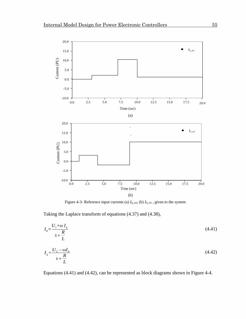
Internal Model Design for Power Electronic Controllers 55
Figure 4-3- Reference input currents (a) Iq_ref, (b) Id_ref , given to the system
0.0 2.5 5.0 7.5 10.0 12.5 15.0 17.5 20.0
-10.0
-5.0
0.0
5.0
10.0
15.0
20.0
Iq_ref
Time (sec)
Cu
rren
t (P
U)
Time (sec)
Cu
rren
t (P
U)
0.0 2.5 5.0 7.5 10.0 12.5 15.0 17.5 20.0 -10.0
-5.0
0.0
5.0
10.0
15.0
20.0
Id_ref
(a)
(b)
Taking the Laplace transform of equations (4.37) and (4.38),
1 q
d
+ω =
U II
Rs
L
(4.41)
2 dq
ω=
U II
Rs
L
(4.42)
Equations (4.41) and (4.42), can be represented as block diagrams shown in Figure 4-4.

Internal Model Design for Power Electronic Controllers 56
Iq
ω
+
U1 Id
+
Transfer
Function of
(4.41)
Id
+
U2Iq-
ω
Transfer
Function of
(4.42)
(a)
(b)
Figure 4-4 - Representation of the power system equations (a) (4-41) and (b) (4-42) in block diagrams
The power system equivalent system shown in Figure 4-5 is controlled using the con-
trollers by block diagrams shown by Figure 4-2 and Figure 4-4.
A
B
C
Ea
Eb
Ec
Ia
Ib
Ic
Vc
Va
Vb
Ra
Rb
Rc
La
Lb
Lc
Figure 4-5- Representation of the power system
Figure 4-5 is a representation of the power system and Va, Vb and Vc are the voltages sup-
plied to the system by the converter. Ea, Eb and Ec are the source voltages of the power
system and the system parameter values are shown in Table 4-1.
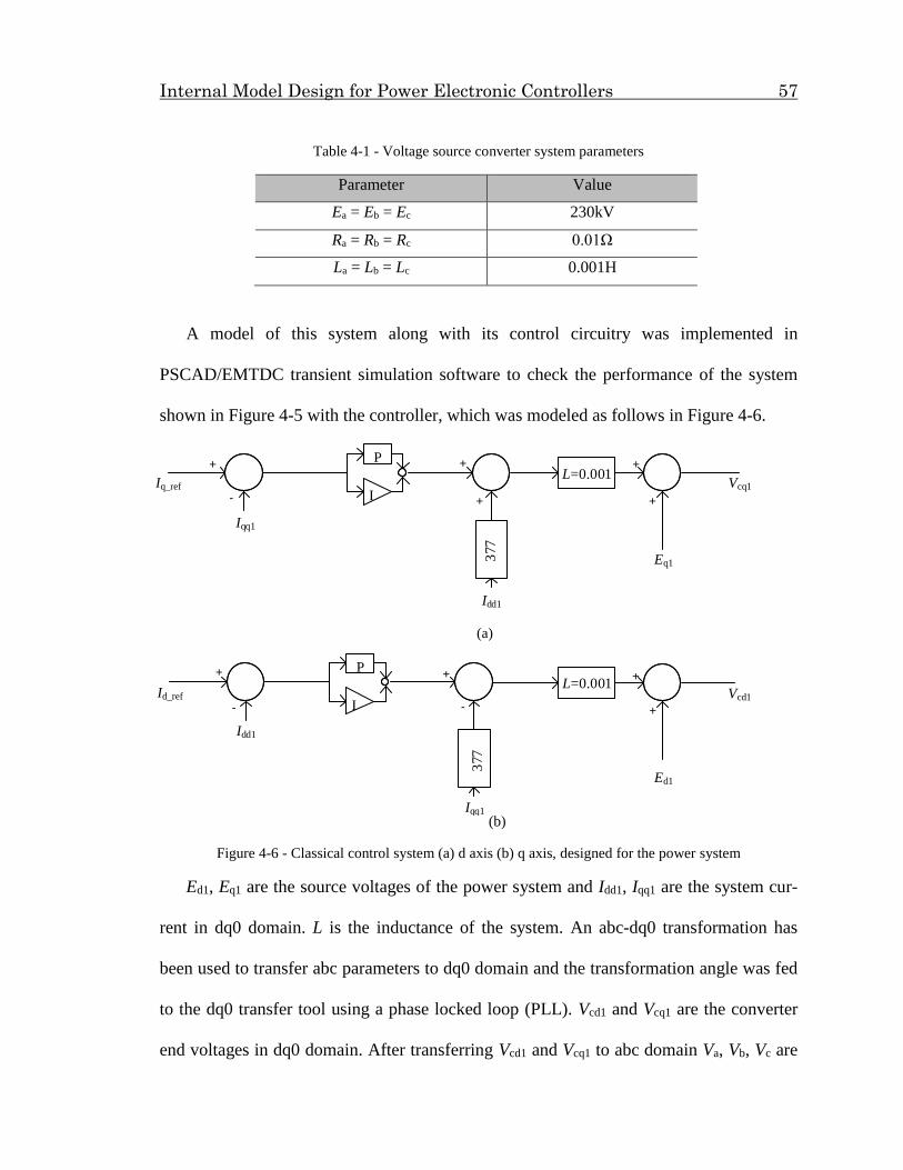
Internal Model Design for Power Electronic Controllers 57
I
P
Ed1
+
+
Vcd1
Iqq1
377
I
P
Vcq1
Eq1
Idd1
377
+
+
+
+
+
-
+
-
+
-
Id_ref
Iq_ref
Iqq1
Idd1
L=0.001
L=0.001
(a)
Table 4-1 - Voltage source converter system parameters
Parameter Value
Ea = Eb = Ec 230kV
Ra = Rb = Rc 0.01Ω
La = Lb = Lc 0.001H
A model of this system along with its control circuitry was implemented in
PSCAD/EMTDC transient simulation software to check the performance of the system
shown in Figure 4-5 with the controller, which was modeled as follows in Figure 4-6.
(b)
Figure 4-6 - Classical control system (a) d axis (b) q axis, designed for the power system
Ed1, Eq1 are the source voltages of the power system and Idd1, Iqq1 are the system cur-
rent in dq0 domain. L is the inductance of the system. An abc-dq0 transformation has
been used to transfer abc parameters to dq0 domain and the transformation angle was fed
to the dq0 transfer tool using a phase locked loop (PLL). Vcd1 and Vcq1 are the converter
end voltages in dq0 domain. After transferring Vcd1 and Vcq1 to abc domain Va, Vb, Vc are

Internal Model Design for Power Electronic Controllers 58
Figure 4-7 – Reference and system currents (a) in q axis, (b) in d axis, of the classical control system
supplied to the power system as shown in Figure 4-5. PI controllers of the system were
tuned using trial and error to obtain the system current similar to the reference current in-
put. The above simulation cases were simulated for 20 seconds and results shown in
Figure 4-7 were obtained.
(a)
(b)
Idd1 and Iqq1 are the system current in dq0 frame and Id_ref and Iq_ref are the reference
current input to the controller. According to the Figure 4-7, it can be seen that even
Time (sec)
Cu
rren
t (P
U)
0.0 2.5 5.0 7.5 10.0 12.5 15.0 17.5 20.0 -10.0
-5.0
0.0
5.0
10.0
15.0
20.0
Idd1
Id_ref
0.0 2.5 5.0 7.5 10.0 12.5 15.0 17.5 20.0
-10.0
-5.0
0.0
5.0
10.0
15.0
20.0
Iqq1
Iq_ref
Time (sec)
Cu
rren
t (P
U)

Internal Model Design for Power Electronic Controllers 59
though there is a small transient period, the output currents follow the reference value as
expected and the system is decoupled accurately.
4.4 Mathematical modeling of the internal model
design
As described in Chapter 3, an internal model is designed to improve the performance of
the classical decoupled control system. System parameter values were used as shown in
Table 4-1. To develop an internal model design, two methods are used.
I
P
Iq
377
++
-
Id_ref
Id
U1
+
Iq
377
+
Id-
Transfer
Function of
(4.41)P1
(a)
I
P
Id
377
++
-
Iq_ref
Iq
U2
+
Id
377
+
Iq
-P2
Transfer
Function of
(4.42)
(b)
Figure 4-8 - Representation of the classical control system (a) d axis (b) q axis, with equivalent model of
the power system

Internal Model Design for Power Electronic Controllers 60
4.4.1 Method 1: (control system with an internal model design)
Figure 4-8 is used to calculate state variables Id and Iq that would be generated in the
power system at a given time. The following equations were then developed by writing
equivalences to Id, Iq and U1, U2.
q 2 d
1=( ω )
( )
I U IR
sL
(4.43)
d 1 q
1=( ω )
( )
I U IR
sL
(4.44)
2 d 2ω P I U so that 2 2 d= ω P U I (4.45)
1 q 1- ω =P I U so that 1 1 q= ω P U I (4.46)
Therefore to predict the output currents Id and Iq considering equations (4.43) and
(4.44), it can be seen that by multiplying equations (4.45) and (4.46) by ( s +R
L) factors Iq
and Id can be obtained.
Therefore the predictive state variables can be written as:
2 q
1=
( )
P IR
sL
(4.47)
1 d
1=
( )
P IR
sL
(4.48)

Internal Model Design for Power Electronic Controllers 61
The modified control system with the predictive state feedback is shown as in Figure 4-9.
Iq_ref
Id_ref
+
-
+
-
+
-
+
+
+
+
377
Eq
Vcq
377
Vcd
+
+
Ed
1sT
1sT
Iqq
Idd
+
-
+
-
L=0.001Gq=0.1
Transfer
Function of
(4.47)
L=0.001Gd=0.1
Transfer
Function of
(4.48)
(a)
(b)
Figure 4-9 – (a) d axis (b) q axis, modified control systems with internal model designs
Ed and Eq are the source voltages of the power system and Idd, Iqq are the system cur-
rents in dq0 domain. L, Gd, and Gq are the inductance of the system and the proportional
gains of d axis and q axis current controllers, respectively. An abc dq0 transformation has
used to transfer abc parameters to dq0 domain in PSCAD/EMTDC simulation software.
The transformation angle was fed to the dq0 transfer tool using a phase locked loop
(PLL). Vcd and Vcq are the converter end voltages in dq0 domain. After transferring Vcd
and Vcq to abc domain Va, Vb, Vc are supplied to the power system. PI controllers of the
system were tuned using trial and error to obtain the system current similar to the refer-
ence current input. This simulation case was simulated for 20 seconds and results shown
in Figure 4-10 were obtained. Reference currents shown in Figure 4-3 were given to the
modified controller so that a clear comparison over each case can be achieved.

Internal Model Design for Power Electronic Controllers 62
-2.0
0.0
2.0
4.0
6.0
8.0
10.0
12.0
Iq_re f
0.0 2.5 5.0 7.5 10.0 12.5 15.0 17.5 20.0
IqqC
urr
en
t (P
U)
Time (sec)
(a)
0.0 2.5 5.0 7.5 10.0 12.5 15.0 17.5 20.0 -4.0
-2.0
0.0
2.0
4.0
6.0
8.0
10.0
12.0
Id_re f
Idd
Time (sec)
Cu
rren
t (P
U)
(b)
Figure 4-10 - Reference currents given to the controllers and the system currents (a) in q axis, (b) in d axis
Idd and Iqq are the system currents in dq0 frame and Id_ref and Iq_ref are the reference
current input to the modified controller. According to the Figure 4-10, it can be seen that
the output currents follow the reference values as expected and the system is decoupled
accurately. Therefore it can be concluded that the new controller has provided expected
results.

Internal Model Design for Power Electronic Controllers 63
4.4.2 Method 2: (control system with the state observer)
In this method, to provide the state feed back to the controller in this particular applica-
tion, a different state observer concept has been used [28]. This method has been dis-
cussed in detail in chapter 3 with two examples.
In designing of state observer process, first assumption was that all the states are
available for the feedback.
The system equation for this particular application can be stated as follows:
d
d 1
qq 2
-1 0
0 1- -
dI RI Udt L
IdI UR
Ldt
(4.49)
By substituting the values from Table 4-1 in to equation (4.49),
1 1
2 2
-10 377= +
-377 -10
u
u
xx
x (4.50)
1
2
1 0=
0 1y
x
x (4.51)
To design the observer, the gain matrix and other parameters were calculated as below.
-10 377
=-377 -10
A 1 0
=0 1
C 1 0
=0 1
B
The state observer equation is given bellow.
= + + ( - )u yx Ax B L Cx (4.52)
where x denotes the estimate of the state x and the L matrix is the observer gain matrix

Internal Model Design for Power Electronic Controllers 64
which will be determined as part of the observer design. The estimation error can be writ-
ten as:
( ) = ( ) - ( )t t te x x (4.53)
Taking the time derivative of the error given by equation (4.53),
= - e x x (4.54)
By combining equations (4.52) and (4.54), the following equation can be obtained,
= + - - - ( - )u u ye Ax B Ax B L Cx (4.55)
( ) ( ) ( )t t e A LC e (4.56)
Characteristic equation of equation (4.56) can be written as below,
det (λ - ( - )) = 0I A LC (4.57)
For a faster response with a lower overshoot, suppose the characteristic equations can
be written [40] as:
2 2
n nΔ(λ) = λ + 2ξ λ + (4.58)
where 𝜉 is the damping ratio and n is the angular velocity. According to the dimen-
sions of the system given in this example the gain matrix (L) can be written as:
1 2
3 4
L L
L L
By substituting the values of Table 4-1 in equation (4.57),
1 2
3 4
1 0 -10 377 1 0λ - - =0
0 1 -377 -10 0 1
L L
L L
1 2
3 4
-10 - 377- λ 0- =0
-377 - -10 - 0 λ
L L
L L

Internal Model Design for Power Electronic Controllers 65
1 2
3 4
λ+10+L -377+L=0
377+L λ+10+L
1 4 2 3λ +10 + λ +10 + - -377 + 377 =0L L L L (4.59)
Assume L2 and L4 are 1 (for the simplicity of the calculations)
2
1 1 3Δ λ =λ +λ +21 +11 10+ +376( +377)L L L (4.60)
Let n be 10 and select 𝜉 to be 0.8 for minimal overshoot [40], using equations (4.58)
and (4.60), 𝐿3 and 𝐿1 can be found.
1 21 16L
1 5L and
1 311 10 + +376 ( + 377) =100L L (4.61)
By substituting the value of L1 in to equation (4.61), L3 can be found.
3 376.88L
By substituting the values from Table 4-1 for the observer equation (4.52),
-10 377 1 0 -5 1
= + + - -377 -10 0 1 -376.88 1
u y
x x Cx (4.62)
Taking the Laplace transform of the above equation,
1 1 2 1 1 1 2 2s =-10 + 377 + -5 -21 + -u y yx x x x x
1 2 1 21
+ - 5 + 376=
s + 5
y yu xx (4.63)
And 2 1 2 2 1 1 2 2s =-377 -10 + - 376.88 + 376.88 + - u y yx x X x x
2 2 1 12
+ -376.88 - 0.12=
s +11
y yu xx (4.64)

Internal Model Design for Power Electronic Controllers 66
The modified control system with the predictive state feedback can be shown by Fig-
ure 4-11. The state estimator was designed using the above calculated values.
(a)
(b)
Figure 4-11 - (a) d axis (b) q axis, modified control systems with state observer
Ed, Eq are the source voltages of the power system and Idd, Iqq are the system currents in
dq0 domain. L is the system inductance and Gd1, Gd2, Gq1, Gq2 are the d and q axis current
controller gains.The transformation angle was fed to the dq0 transfer tool using a phase
locked loop (PLL). Vcd and Vcq are the converter end voltages in dq0 domain. After fer-
Id_ref
+
-
+
-
377
Vcd
+
+
Ed
1sT
Idd
+
-
Iqq
L=0.001Gd1=0.01u1
Idd
376
Iqq
-5
u1
+
+
+
+
Transfer
Function of
(4.63)
Gd2=
0.0
00
1
+
-
+
+
+
+
377
Eq
Vcq
1sT
Iqq
+
-
Idd
L=0.001Gq1=0.05u2
Gq2=
0.0
00
1
Idd
-376
.88
Iqq
-0.12
u2
+
+
+
+
Transfer
Function of
(4.64)
Iq_ref

Internal Model Design for Power Electronic Controllers 67
-6.0
-4.0
-2.0
0.0
2.0
4.0
6.0
8.0
10.0
12.0
14.0
0.0 2.0 4.0 6.0 8.0 10.0 12.0 14.0 16.0
Iq_re f
Iqq
Cu
rren
t (P
U)
Time (sec)
0.0 2.0 4.0 6.0 8.0 10.0 12.0 14.0 16.0 -4.0
-2.0
0.0
2.0
4.0
6.0
8.0
10.0
12.0
14.0
Id_re f
Idd
Time (sec)
Cu
rren
t (P
U)
(a)
(b)
ring Vcd and Vcq to abc domain Va, Vb, Vc are supplied to the power system. PI controllers
of the system were tuned to obtain the system current similar to the reference current in-
puts shown in Figure 4-3. These simulation cases were simulated for 20 seconds and the
results shown in Figure 4-12 were obtained.
Figure 4-12 - Reference currents given to the controllers and system currents (a) in q axis, (b) in d axis
Idd and Iqq are the system currents in dq0 frame and Id_ref and Iq_ref are the refrence current
input to the modified controller. According to Figure 4-12, it can be seen that the output
currents of the new controller follow the reference values as expected and the system is
decoupled accurately.

Internal Model Design for Power Electronic Controllers 68
-5.0
-2.5
0.0
2.5
5.0
7.5
10.0
12.5
15.0
17.5
Iqq
Iqq1
Iq_re f
Cu
rren
t (P
U)
Time (sec)2.5 5.0 7.5 10.0 12.5 15.0 17.5 20.0 0.0
0.0 2.5 5.0 7.5 10.0 12.5 15.0 17.5 20.0 -10.0
-5.0
0.0
5.0
10.0
15.0
20.0
Cu
rren
t (P
U)
Time (sec)
Idd
Idd1
Id_re f
(b)
4.5 Simulation results
Simulation cases shown by Figures 4-6 and 4-9 were simulated for 20 seconds where
each case was fed with references shown in Figure 4-3, plotted in the same graph shown
by Figure 4-13, so that a clear comparison over each case can be achieved.
(a)
Figure 4-13 - Reference currents and the system currents (a) in q axis, (b) in d axis when the classical con-
troller and the modified controller (using method 1) are used
Idd and Iqq are the system currents in dq0 frame when the Id_ref and Iq_ref are given as
the reference input to the modified controller with the predictive control loop using

Internal Model Design for Power Electronic Controllers 69
Curr
ent
(PU
)
-7.5
-5.0
-2.5
0.0
2.5
5.0
7.5
10.0
12.5
15.0
17.5
Iqq
Iqq1
Iq_re f
0.0 2.0 4.0 6.0 8.0 10.0 12.0 14.0 16.0
Cu
rren
t (P
U)
Time (sec)
0.0 2.0 4.0 6.0 8.0 10.0 12.0 14.0 16.0 -10.0
-5.0
0.0
5.0
10.0
15.0
20.0
Idd
Idd1
Id_re f
Time (sec)
(a)
(b)
method 1 calculation and Idd1 and Iqq1 are the system current in dq0 frame when the clas-
sical controller is connected to the system.
Simulation cases shown by Figures 4-6 and Figure 4-11 were simulated for 20 sec-
onds where each case was fed with references shown in Figure 4-3, plotted in the same
graph shown by the following figures so that a clear comparison over each case can be
achieved.
Figure 4-14 - Reference currents and the system currents (a) in q axis, (b) in d axis when the classical con-
troller and the modified controller (using method 2) are used

Internal Model Design for Power Electronic Controllers 70
Idd and Iqq are the system currents in dq0 frame when the Id_ref and Iq_ref are given as
the reference input to the modified controller which comprised with the predictive control
loop using method 2 calculations and Idd1 and Iqq1 are the system current in dq0 frame
when the classical controller is connected to the system.
According to Figures 4-13 and 4-14, it can be see that all the controllers have deliv-
ered expected results and the controller with the state estimator which was calculated us-
ing the procedure described in method 1, has given better results compared to other con-
trol methods. When considering the transient period, the classical control system has lot
of fluctuations whereas the controller with the internal model, which was designed using
method 1, follows the reference without unexpected fluctuations. The controller designed
using the calculations described in method 2 has also provided better results compared to
the classical control system but could not reach the performance level provided by the
controller designed using the calculations described in method 1.
To check the behaviour of the system current when the modified controller was con-
nected to the power system over the classical controller scenario, under different circum-
stances the following simulations shown in Figure 4-15 were carried out using
PSCAD/EMTDC software.
4.5.1 System current behavior after adding a filter to the system
Filtering of output parameters, which are extracted from the system to feed to the control-
ler, is an external condition that can cause time delay. Therefore in this section a filter
which provides 0.5ms time delay in the feedback system has been added to the system.

Internal Model Design for Power Electronic Controllers 71
-10.0
-5.0
0.0
5.0
10.0
15.0
20.0
Id_re f
Idd1_fi ltere d
0.0 2.5 5.0 7.5 10.0 12.5 15.0 17.5 20.0
Time (sec)
Cu
rren
t (P
U)
Time (sec)
Cu
rren
t (P
U)
-7.5
-5.0
-2.5
0.0
2.5
5.0
7.5
10.0
12.5
15.0
17.5
2.5 5.0 7.5 10.0 12.5 15.0 17.5 20.0 0.0
Iq_re f
Iqq1_fi ltered
The following simulation results were obtained to observe the behaviour of the classical
controller and the modified controllers.
(a)
(b)
Figure 4-15 - Reference currents and the filtered system currents (a) in q axis, (b) in d axis when the classi-
cal controller is used
Idd1_filtered and Iqq1_filtered are the system current in dq0 frame when the Id_ref and Iq_ref
are given as the reference current inputs to the classical controller. Comparing Figure 4-
15 with Figure 4-7 it can be observed that, with the delay in the system due to the filter,
the classical controller has given unexpected results comprised of a lot of fluctuations and
lack of decoupling capability.

Internal Model Design for Power Electronic Controllers 72
-4.0
-2.0
0.0
2.0
4.0
6.0
8.0
10.0
12.0
2.5 5.0 7.5 10.0 12.5 15.0 17.5 20.0 0.0
Time (sec)
Cu
rren
t (P
U)
Id_re f
Idd_fi ltered
0.0 2.5 5.0 7.5 10.0 12.5 15.0 17.5 20.0 -2.0
0.0
2.0
4.0
6.0
8.0
10.0
12.0
Time (sec)
Cu
rren
t (P
U) Iq_re f
Iqq_fi ltered
(a)
(b)
Figure 4-16 - Reference currents and the filtered system currents (a) in q axis, (b) in d axis, of the modified
controller designed using method 1
Idd_filtered and Iqq_filtered are the system current in dq0 frame when the Id_ref and Iq_ref are
given as the reference current inputs to the modified controller which was designed as
described in method 1. Comparing Figure 4-10 with Figure 4-16 it can be observed that,
even with the delay in the system due to the filter, the controller modified using method
1, has given expected results.

Internal Model Design for Power Electronic Controllers 73
0.0 2.0 4.0 6.0 8.0 10.0 12.0 14.0 16.0 -4.0
-2.0
0.0
2.0
4.0
6.0
8.0
10.0
12.0
14.0
Time (sec)
Cu
rren
t (P
U)
Id_re f
Idd_fi ltered
Time (sec)
Cu
rren
t (P
U)
0.0 2.0 4.0 6.0 8.0 10.0 12.0 14.0 16.0 -6.0
-4.0
-2.0
0.0
2.0
4.0
6.0
8.0
10.0
12.0
14.0
Iq_re f
Iqq_fi ltered
(a)
(b)
Figure 4-17 - Reference currents and the filtered system currents (a) in q axis, (b) in d axis, of the modified
controller designed using method 2
Idd_filtered and Iqq_filtered are the system current in dq0 frame when the Id_ref and Iq_ref are
given as the reference current inputs to the modified controller which was designed as
described in method 2. Comparing Figure 4-12 with Figure 4-17 it can be observed that,
with the delay in the system the controller modified using method 2, has given better re-
sults compared to the classical control system but it is not decoupled as desired. Further-

Internal Model Design for Power Electronic Controllers 74
-7.5
-5.0
-2.5
0.0
2.5
5.0
7.5
10.0
12.5
15.0
17.5
2.5 5.0 7.5 10.0 12.5 15.0 17.5 20.0 0.0
Time (sec)
Curr
ent
(PU
)
Iq_re f
Iqq1
0.0 2.5 5.0 7.5 10.0 12.5 15.0 17.5 20.0 -10.0
-5.0
0.0
5.0
10.0
15.0
20.0
Time (sec)
Cu
rren
t (P
U)
Id_re f
Idd1
more it can be seen that the controller modified using method 1 has higher decoupling
capability and less transients compared to controller designed as described by method 2.
4.5.2 System current behavior after changing the inductance of
the system by 1 percent without adding the filter
(a)
(b)
Figure 4-18 - Reference currents and the system currents (a) in q axis, (b) in d axis when the classical con-
troller is used (with 1% inductance change and without adding a filter)
Idd1 and Iqq1 are the system current in dq0 frame when the Id_ref and Iq_ref are given as the
reference current inputs to the classical controller. When comparing Figure 4-18 with

Internal Model Design for Power Electronic Controllers 75
Time (sec)
Cu
rren
t (P
U)
-2.0
0.0
2.0
4.0
6.0
8.0
10.0
12.0
2.5 5.0 7.5 10.0 12.5 15.0 17.5 20.0 0.0
Iq_re f
Iqq
Curr
ent
(PU
)
0.0 2.5 5.0 7.5 10.0 12.5 15.0 17.5 20.0 -4.0
-2.0
0.0
2.0
4.0
6.0
8.0
10.0
12.0
Time (sec)
Id_re f
Idd
Figure 4-7 it can be observed that, with the inductance change in the system, the classical
controller has given unexpected results including unpredicted fluctuations and lack of de-
coupling capability.
(a)
(b)
Figure 4-19 - Reference currents and the system currents (a) in q axis, (b) in d axis, of the modified control-
ler designed using method 1 (with 1% inductance change and without adding a filter)
Idd and Iqq are the system current in dq0 frame when the Id_ref and Iq_ref are given as
the reference current inputs to the modified controller which was designed using the cal-
culations described by method 1. The inductance was changed by 1 percent from its orig-

Internal Model Design for Power Electronic Controllers 76
Time (sec)
Curr
ent
(PU
)
-6.0
-4.0
-2.0
0.0
2.0
4.0
6.0
8.0
10.0
12.0
14.0
0.0 2.0 4.0 6.0 8.0 10.0 12.0 14.0 16.0
Iq_re f
Iqq
Curr
ent
(PU
)
Time (sec)
0.0 2.0 4.0 6.0 8.0 10.0 12.0 14.0 16.0 -4.0
-2.0
0.0
2.0
4.0
6.0
8.0
10.0
12.0
14.0
Id_re f
Idd
inal value. Comparing Figure 4-19 with Figure 4-10 it can be observed that, even with the
inductance change in the system, the modified controller has given the expected results.
(a)
(b)
Figure 4-20 - Reference currents and the system currents (a) in q axis, (b) in d axis, of the modified control-
ler designed using method 2 (with 1% inductance change and without adding the filter)
Idd and Iqq are the system current in dq0 frame when the Id_ref and Iq_ref are given as the
reference current inputs to the modified controller designed using the calculations de-
scribed by method 2. Comparing Figure 4-20 with Figure 4-12 it can be observed that,
with the inductance change in the system, the modified controller has given unexpected
results including unpredicted fluctuations and lack of decoupling capability. The control-

Internal Model Design for Power Electronic Controllers 77
(b)
Curr
ent
(PU
)
Time (sec)
-5.0
-2.5
0.0
2.5
5.0
7.5
10.0
12.5
15.0
17.5
0.0 2.5 5.0 7.5 10.0 12.5 15.0 17.5 20.0
Iq_re f
Iqq1
Cu
rren
t (P
U)
0.0 2.5 5.0 7.5 10.0 12.5 15.0 17.5 20.0 -7.5
-5.0
-2.5
0.0
2.5
5.0
7.5
10.0
12.5
15.0
17.5
Time (sec)
Id_re f
Idd1
(a)
ler performance modified using method 2 has deteriorated from its reference inputs given
to the controller.
4.5.3 System current behavior after changing the inductance of
the system by 5 percent without adding the filter
Figure 4-21 - Reference currents and the system currents (a) in q axis, (b) in d axis when the classical con-
troller is used (with 5% inductance change and without adding the filter)
Idd1 and Iqq1 are the system current in dq0 frame when the Id_ref and Iq_ref are given as the
reference current inputs to the classical controller. Comparing Figure 4-21 with Figure 4-
7 it can be observed that, with the 5 percent inductance change in the system, the classical

Internal Model Design for Power Electronic Controllers 78
-2.0
0.0
2.0
4.0
6.0
8.0
10.0
12.0
0.0 2.5 5.0 7.5 10.0 12.5 15.0 17.5 20.0
Curr
ent
(PU
)
Time (sec)
Iq_re f
Iqq
Curr
ent
(PU
)
Time (sec)
0.0 2.5 5.0 7.5 10.0 12.5 15.0 17.5 20.0 -4.0
-2.0
0.0
2.0
4.0
6.0
8.0
10.0
12.0
Id_re f
Idd
controller has given unexpected results comprised of unpredicted fluctuations in the out-
put and lack of decoupling capability.
(a)
(b)
Figure 4-22 - Reference currents and the system currents (a) in q axis, (b) in d axis, of the modified control-
ler designed using method 1 (with 5% inductance change and without adding the filter)
Idd and Iqq are the system currents in dq0 frame when the Id_ref and Iq_ref are given as
the reference current inputs to the modified controller which was designed using the cal-
culations described by method 1. The inductance has been changed by 5 percent from
their original values. Comparing Figure 4-22 with Figure 4-10 it can be observed that,
even with the inductance change in the system by 5 percent, the modified controller has
given the expected results.

Internal Model Design for Power Electronic Controllers 79
-7.5
-5.0
-2.5
0.0
2.5
5.0
7.5
10.0
12.5
15.0
17.5
0.0 2.5 5.0 7.5 10.0 12.5 15.0 17.5 20.0
Time (sec)
Curr
ent
(PU
)
Iq_re f
Iqq1
0.0 2.5 5.0 7.5 10.0 12.5 15.0 17.5 20.0 -10.0
-5.0
0.0
5.0
10.0
15.0
20.0
Time (sec)
Curr
ent
(PU
)
Id_re f
Idd1
(a)
(b)
4.5.4 System current behavior after changing the inductance of
the system by 10 percent without adding the filter
Figure 4-23 - Reference currents and the system currents (a) in q axis, (b) in d axis when the classical con-
troller is used (with 10% inductance change and without adding the filter)
Idd1 and Iqq1 are the system current in dq0 frame when the Id_ref and Iq_ref are given as
the reference current inputs to the classical controller. Comparing Figure 4-23 with Fig-
ure 4-7 it can be observed that, with the 10 percent inductance change in the system, the
classical controller has given unexpected results comprised of unpredicted fluctuations
and lack of decoupling capability. When comparing the system current performances

Internal Model Design for Power Electronic Controllers 80
Time (sec)
-2.0
0.0
2.0
4.0
6.0
8.0
10.0
12.0
2.5 5.0 7.5 10.0 12.5 15.0 17.5 20.0 0.0
Cu
rren
t (P
U)
Iq_re f
Iqq1
Time (sec)
Cu
rren
t (P
U)
0.0 2.5 5.0 7.5 10.0 12.5 15.0 17.5 20.0 -4.0
-2.0
0.0
2.0
4.0
6.0
8.0
10.0
12.0
Id_re f
Idd
with 5 percent inductor change and 10 percent inductor change, it can be clearly seen that
when the change of the system parameter increased, the unexpectancy of the controller
results has also increased.
(a)
(b)
Figure 4-24 - Reference currents and the system currents (a) in q axis, (b) in d axis, of the modified control-
ler designed using method 1 (with 10% inductance change and without adding a filter)
Idd and Iqq are the system current in dq0 frame when the Id_ref and Iq_ref are given as the
reference current inputs to the modified controller which was designed using the calcula-
tions described by method 1. The inductance has been changed by 10 percent from its
original value. Comparing Figure 4-22 with Figure 4-10 it can be observed that, even

Internal Model Design for Power Electronic Controllers 81
(a)
Time (sec)
-10.0
-5.0
0.0
5.0
10.0
15.0
20.0
0.0 2.5 5.0 7.5 10.0 12.5 15.0 17.5 20.0
Cu
rren
t (P
U)
Id_re f
Idd1_fi ltered
Time (sec)
Cu
rren
t (P
U)
0.0 2.5 5.0 7.5 10.0 12.5 15.0 17.5 20.0 -7.5
-5.0
-2.5
0.0
2.5
5.0
7.5
10.0
12.5
15.0
17.5
Iq_re f
Iqq1_fi ltere d
(b)
with the inductance change in the system by 10 percent, the controller modified using
method 1, has given the expected results.
4.5.5 System current behavior after changing the inductance of
the system by 10 percent with the filter
Figure 4-25 - Reference currents and the system currents (a) in q axis, (b) in d axis when the classical con-
troller is used (with 10% inductance change and after adding a filter)
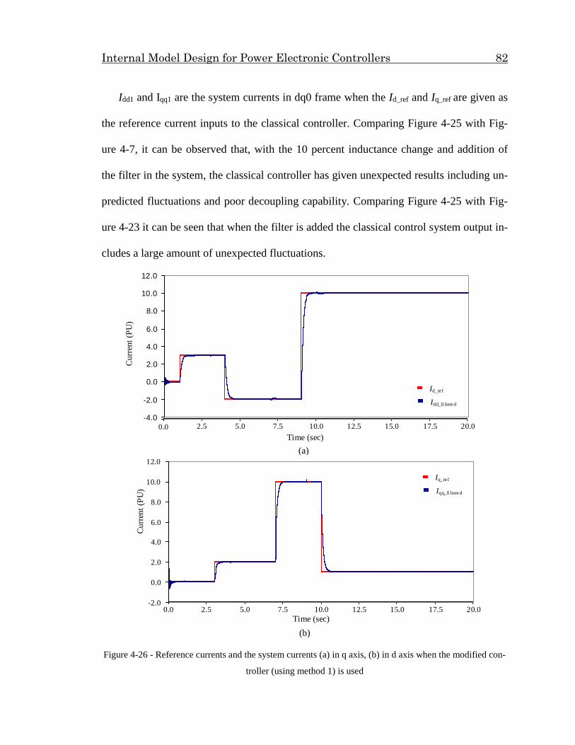
Internal Model Design for Power Electronic Controllers 82
(a)
Time (sec)
Curr
ent
(PU
)
-4.0
-2.0
0.0
2.0
4.0
6.0
8.0
10.0
12.0
2.5 5.0 7.5 10.0 12.5 15.0 17.5 20.0 0.0
Id_re f
Idd_fi ltered
0.0 2.5 5.0 7.5 10.0 12.5 15.0 17.5 20.0 -2.0
0.0
2.0
4.0
6.0
8.0
10.0
12.0
Time (sec)
Curr
ent
(PU
)
Iq_re f
Iqq_fi ltered
Idd1 and Iqq1 are the system currents in dq0 frame when the Id_ref and Iq_ref are given as
the reference current inputs to the classical controller. Comparing Figure 4-25 with Fig-
ure 4-7, it can be observed that, with the 10 percent inductance change and addition of
the filter in the system, the classical controller has given unexpected results including un-
predicted fluctuations and poor decoupling capability. Comparing Figure 4-25 with Fig-
ure 4-23 it can be seen that when the filter is added the classical control system output in-
cludes a large amount of unexpected fluctuations.
(b)
Figure 4-26 - Reference currents and the system currents (a) in q axis, (b) in d axis when the modified con-
troller (using method 1) is used

Internal Model Design for Power Electronic Controllers 83
Idd and Iqq are the system current in dq0 frame when the Id_ref and Iq_ref are given as the
reference current inputs to the modified controller which was designed using the calcula-
tions described by method 1. The inductance has been changed from 10 percent and a
0.5ms delay was added to the feedback system. Comparing Figure 4-26 with Figure 4-10
it can be observed that, even with the inductance change in the system by 10 percent with
the filter, the modified controller has given expected results.
As per the simulation results shown in this chapter, it can be concluded that the inter-
nal model based tracking technique which has been developed for this particular applica-
tion has the capability of handling uncertainties in the plant parameters as well as the
changes of the trajectory. Time delays caused by exogenous conditions such as adding
filters to the system can also be compensated. More over the new controller can provide
expected results even when there is simultaneous system unexpected conditions.

Internal Model Design for Power Electronic Controllers 84
Chapter 5
Vector Controlled Induction Motor
Drives
Electric motors are used in a wide spectrum of power applications ranging from fraction
of a Watt to several Mega-Watts and are available in different forms such as ac or dc, and
single phase or three phase. DC motors are efficient and because of their characteristics
and controllability, have a large presence in motion control applications. However dc mo-
tors use physical contacts such as commutators and brushes, which frequently require
maintenance due to wear and tear [42]. With the enhancements of power electronic con-
trol strategies, advanced control methods of controlling the torque and speed of ac ma-
chines have been used in many power system applications. Induction motors are com-
monly used in most of the industrial applications, due to the simplicity, high efficiency,
solid construction and other appealing features [43].

Internal Model Design for Power Electronic Controllers 85
Induction motor drives can usually be categorized as the ones based on the steady
state model of the machine and the ones rooted in the dynamic model of the machine. In-
duction motor controllers designed based on steady state observations of the machine
provide acceptable performance only in steady state conditions [44]. The induction motor
controllers developed using a transient model of the machine provide acceptable perfor-
mance under both steady and transient conditions. These control techniques are referred
to as field oriented or vector control methods and allow the electromagnetic torque to fol-
low a reference torque providing higher dynamic performance and faster response [44]-
[49].
5.1 Induction machine model
To develop the machine model a three phase two pole induction machine has been used
and it is assumed to have sinusoidally distributed windings both on the rotor and stator.
astator axis
arotor axis
bstator axis
brotor axis
cstator axis
crotor axis
Figure 5-1 – A three phase two pole induction machine

Internal Model Design for Power Electronic Controllers 86
The flux linkages of the stator and the rotor windings can be expressed by the follow-
ing equation:
sabcs abcssr
Tabcr abcrrsr
Lλ iL=
λ iL(L )
(5.1)
where the stator flux linkage is T
abcs as bs csλ = λ λ λ and the rotor flux linkage is:
T
abcr ar br crλ = λ λ λ .
The voltage equations can be expressed as shown below:
abcs s abcs abcsV r i p (5.2)
abcr r abcr abcrV r i p (5.3)
where rr and sr are the rotor and stator resistance and p is the time derivative.
Using Park’s transformation the above two sets of equations can be transformed into
a dq0 frame where the location of the frame is specified by ɵ as per the Figure 5-2.
The transformation matrix for the stator quantities and rotor quantities can be shown by
the following matrices:
s
2π 2πcos(θ) cos(θ- ) cos(θ+ )
3 3
2 2π 2πK = sin(θ) sin(θ- ) sin(θ+ )
3 3 3
1 1 1
2 2 2
and r
2π 2πcos(β) cos(β- ) cos(β+ )
3 3
2 2π 2πK = sin(β) sin(β- ) sin(β+ )
3 3 3
1 1 1
2 2 2
where r is the angle between the rotor a axis and the q axis of the reference
frame.
Let the rotor speed and the stator speed be ωr and ωs (elect. rad/s), respectively.

Internal Model Design for Power Electronic Controllers 87
astator axis
arotor axis
bstator axis
cstator axis
crotor axis d axis
q axis
Figure 5-2 – Reference frame for transformation
Using equation (5.1) and the transformation matrices the following equations can be de-
rived:
1 1
qd0s s s s qd0s s sr r qd0s= K L K i K L K i
T 1 1
qd0r r sr s qd0s r r r qd0s= K L K i K L K i
qs ls M qs M qr= ( )L L i L i (5.4)
ds ls M ds M dr= ( )L L i L i (5.5)
0s ls 0s= L i (5.6)
qr lr M qr M qs= ( )L L i L i (5.7)
dr lr M dr M ds= ( )L L i L i (5.8)

Internal Model Design for Power Electronic Controllers 88
0r lr 0r= L i (5.9)
The rotor and stator voltage equations can be derived as shown below:
qs s qs ds qs= ωd
V r idt
(5.10)
ds s ds qs ds= d
V r idt
(5.11)
0 0 0= s s s s
dV r i
dt (5.12)
As the rotor is short circuited its voltage equations will be identical to zero.
qr r qr r dr qr= ( ) = 0d
V r idt
(5.13)
dr r dr r qr dr= ( ) = 0d
V r idt
(5.14)
0r r 0r 0r= d
V r idt (5.15)
The torque equation can be derived in the new reference frame as below:
Me qs dr ds qr
M lr
3 PT ( )
2 2
Li i
L L
(5.16)
where P is the number of poles.
5.2 Vector control methodology
When one closely examines the torque equation (5.16) of the induction machine, it can be
seen that the electric torque is generated by the interaction between the stator current vec-
tor s qs dsi = i i and the rotor flux r qr drλ = λ λ . In this vector control strategy the d ax-

Internal Model Design for Power Electronic Controllers 89
is of the reference frame is aligned with the d axis of the rotor flux vector. Rotor flux is a
single entity; therefore the q component of the rotor flux becomes zero.
qr 0
Therefore equation (5.16) can be simplified to:
Me qs dr
M lr
3 PT ( )
2 2
Li
L L
(5.17)
As per this equation it can be observed that the torque is produced as a result of the
armature current and the rotor flux which are 90° apart. The stator current consists of two
current components ids and iqs. The d axis current component (ids) will be along with the
rotor flux and adjusts the field, whereas the q axis current component (iqs), which is per-
pendicular to the flux, will regulate the torque.
Given qr 0 let dr 0i
By substituting values for equation (5.8), the following expression can be obtained.
2
Me qs ds
M lr
3 PT ( )
2 2
Li i
L L
(5.18)
With the two assumptions made earlier it can be seen that the induction machine be-
haviour has become similar to a DC machine, and the following equations can be de-
rived:
dr r dr dr r qr( ) 0d
V r idt (5.19)
From equation (5.8) and (5.19),
r dr lr M dr M ds(( ) ) 0d
r i L L i L idt
(5.20)

Internal Model Design for Power Electronic Controllers 90
dsr dr lr M dr M( )
didr i L L i L
dt dt (5.21)
As per the equation (5.21) it can be seen that, to adjust the field at a given value if the
d-axis stator current (ids) is kept constant then the d-axis rotor current will tend to zero.
5.3 Implementation of the vector control strategy
To implement this control methodology, correct placement of the reference frame has ob-
tained using the rotor voltage equations as shown below:
r qr qr r dr( ) 0d
r idt (5.22)
Therefore,
qr
r r
dr
ir
(5.23)
where ω is the instantaneous speed of the reference frame in electrical rad/s.
With the two assumptions made earlier using equation (5.7):
qr lr M qr M qs( ) 0L L i L i
Therefore,
Mqr qs
lr M
Li i
L L
(5.24)
From equation (5.8),
dr M dsL i (5.25)
After combining equations (5.23), (5.24) and (5.25),

Internal Model Design for Power Electronic Controllers 91
qs_refrr
lr M ds_ref
ir
L L i
(5.26)
where qs_refi and ds_refi are the reference values provided to the converter to drive the mo-
tor.
d
dt
Therefore by integrating the speed (ω) over time, the required angle for trans-
formation can be obtained.
By substituting the expression to speed from equations (5.22) and (5.14) following equa-
tions can be derived:
qs_refrr qr qr dr
lr M ds_ref
0ird
r idt L L i
(5.27)
qs_refrr dr dr qr
lr M ds_ref
0ird
r idt L L i
(5.28)
By finding iqr and λdr from equations (5.7) and (5.8):
Mqr qr qs_ref
lr M lr M
1 Li i
L L L L
(5.29)
dr lr M dr M ds_ref( )L L i L i (5.30)
Using the above equations, the following system equations can be derived,
qr qs_refrqr r dr
lr M ds_ref
=d ir
r idt L L i
(5.31)
qs_ref ds_refdr r r Mqr dr2
lr M ds_ref lr M lr M
=( )
i didi r r Li
dt L L i L L L L dt
(5.32)

Internal Model Design for Power Electronic Controllers 92
As per the above equations it can be seen that the d axis current of the rotor and the q
axis flux of the rotor will vanish to zero when the stator d-axis current is kept con-
stant. This will satisfy the conditions for the vector control as it is assumed the q-axis ro-
tor flux is zero, and the d-axis rotor current is zero resulting in the d-axis stator current
being the only means to adjust the field. A simple block diagram of the control method is
shown below. To yield the required angle for the qd0 transformation speed can be inte-
grated over time. This methodology only measures the speed of the machine and other
parameters are estimated. Torque command is generated as a function of speed error
(ω_ref - ωr) as shown below.
I+
-
ω _ref
ωr
TK
Figure 5-3 – Torque command generator
A simple block diagram of the indirect vector control is shown Figure 5-4.
IMCurrent
controller
Inverse park
transformation
+
-
ia_ref
ib_ref
ic_refiqs_ref
ids_ref
PIω_ref
+
ωr
ωs
ωr
Figure 5-4 – Induction vector control schematic diagram

Internal Model Design for Power Electronic Controllers 93
Figure 5-4 illustrates a summary of generating a three phase stator current to the in-
duction motor. The above case has been designed and simulated using the
PSCAD/EMTDC software and the induction machine drive system parameters are given
bellow.
Table 5-1 - Induction motor Drive system parameters
Parameter Value
Machine Voltage 2300 V
Machine Power 500 hp
Machine Frequency 60 Hz
J 11.06 Kg.m2
Stator resistance - Rs 0.262 Ω
Xls 1.206 Ω
XM 54.02 Ω
Xlr 1.206 Ω
Rotor resistance - Rr 0.187 Ω
Pole 4
Input Voltage 3900 V
Input Frequency 60 Hz
Two major parameters in a machine drive system are the machine speed and the torque,
which are regulated using a PI controller in this control strategy. Therefore the gain and
the time constant of the controller should be carefully tuned to obtain the expected results
which is to follow the changes in a reference frame in this particular drive system.

Internal Model Design for Power Electronic Controllers 94
Figure 5-5 – PSCAD/EMTDC simulation for indirect vector control of induction motor
When the case study shown in Figure 5-5 is simulated using the PSCAD/EMTDC soft-
ware, the following results were obtained.
Time (sec)
10 20 30 40 50 60 70 80 90 100 -0.3k
0.0
0.3k
0.5k
0.8k
1.0k
1.3k
1.5k
1.8k
2.0k
Set Speed
Machine Speed
Spee
d (
rpm
)
Figure 5-6 – Set speed and the machine actual speed
As per Figure 5-6 it can be seen that the machine speed has followed the set speed.
Therefore it can be concluded that the PI controller is well tuned. When the machine
speed is closely examined it can be seen that every time the set speed changes there is a
transient in the machine speed as shown in Figure 5-7.

Internal Model Design for Power Electronic Controllers 95
Time (sec)
Spee
d (
rpm
)
0.990 1.000 1.010 1.020 1.030 1.040 1.70k
1.73k
1.75k
1.77k
1.80k
1.83k
1.85k
1.88k
1.90k
1.93k
1.95k
Set Speed
Machine Speed
Figure 5-7 – Set speed and the actual speed of the machine
As per Figure 5-7, the reference machine set speed has changed to 1800 rpm but it
can be seen that the machine speed has increased up to 1925 rpm before settling to the
reference point and it has taken 0.022 seconds to get settled.
5.3 Addition of the internal model to the indirect
vector control of the induction machine
As described in Chapter 3 a controller designed with an internal model is able to secure
asymptotic decay to zero of the tracking error for every possible trajectory and it can per-
form robustly with respect to parameter uncertainties of the system. a simple internal
model was added to the induction machine controller which is discussed in Section 5.2 to
improve its performance. As described in Section 3.2, the internal model design is de-
signed for the induction motor.
Referring to equation (3.15),

Internal Model Design for Power Electronic Controllers 96
t
1
0
( ) = - ( ) - ( )u t K e d t 2K x
where u(t) is the input to the system and e(t) is the error of that particular time and x(t) is
the state of the system. In this scenario the speed of the machine is considered to be the
state. Therefore the modification shown in Figure 5-8 has been made in the control sys-
tem.
I
ω
K2
+
-
+
-
ω _ref
ωr
U(t)K1
Figure 5.8 - Modified input to the system
Then the gains of the modified controller were tuned to achieve the expected results
and following simulations results shown in Figure 5-9 were obtained.
Time (sec)
Spee
d (
rpm
)
0 10 20 30 40 50 60 70 80 90 100 -0.3k
0.0
0.3k
0.5k
0.8k
1.0k
1.3k
1.5k
1.8k
2.0k
Set Speed
Machine Speed
Figure 5-9 - Set speed and the machine actual speed with the modified controller
As per Figure 5-9 it can be seen that the machine speed has followed the set speed.
With close examination of the machine speed it can be seen that every time when the set

Internal Model Design for Power Electronic Controllers 97
speed changes there is not much of a transient compared to Figure 5-6. This can be clear-
ly seen in Figure 5-10.
Time (sec)
Set Speed
Machine Speed
Sp
eed
(rp
m)
0.960 0.980 1.000 1.020 1.040 1.060 1.080 1.750k
1.760k
1.770k
1.780k
1.790k
1.800k
1.810k
1.820k
Figure 5-10 - Set speed and the actual speed of the machine with the modified
As per the Figure 5-10, the reference machine set speed has changed to 1800rpm
and it can be seen that the machine speed follows the exact reference value and it has tak-
en only 0.018 seconds to get settled. When the two control systems are compared, it can
be clearly seen that the modified control system provides faster response and it closely
follows the reference speed.
5.4 Controller response with and without internal
model to internal parameter change of the machine
When controllers are designed for any power system application or machine drive, most
of the system uncertainties that can occur in real time implementation are not considered.
Therefore those controllers may need to be re tuned to achieve the expected results under
unexpected conditions. In this example, rotor resistance of the machine may change from

Internal Model Design for Power Electronic Controllers 98
its original value. Therefore to check the controller performance, rotor resistance was
changed from half of its value to 1.5 times and the following results were obtained.
Figure 5-11 – Machine speed variation with the rotor resistance change
Figure 5-11 illustrates how the speed of the machine changes with the change of the
rotor resistance. As per the above graph it can be seen that the rotor resistance has been
reduced to 50 percent and then increased by 10 percent until 1.5 percent of the original
resistance. The reference input speed for the controller is 1800 rpm. The maximum tran-
sient machine speed has changed with the rotor resistance change when the normal con-
troller regulate the machine. But with the internal model design it can be seen that the
machine has taken the expected speed for every resistance change.
1780
1800
1820
1840
1860
1880
1900
1920
1940
0 . 5 0 . 7 0 . 9 1 . 1 1 . 3 1 . 5 1 . 7 1 . 9 2 . 1
Mac
hin
e S
pee
d (
rpm
)
Rotor resistance (PU)
Without internal model
With internal model

Internal Model Design for Power Electronic Controllers 99
Figure 5-12 – Time taken to settle with the rotor resistance change
Figure 5-12 illustrates how the time taken to obtain the reference speed of the ma-
chine changes with the change of the rotor resistance. Settling time has changed with the
change of the rotor resistance and when comparing the two cases it can be seen that with
the internal model design, the machine has obtained the expected results much faster than
the classical controller.
0
0.005
0.01
0.015
0.02
0.025
0.03
0.035
0.04
0.045
0 . 5 0 . 7 0 . 9 1 . 1 1 . 3 1 . 5 1 . 7 1 . 9 2 . 1
Tim
e ta
ken
to
set
tle
(s)
Rotor resistance (PU)
Without internal model
With internal model

Internal Model Design for Power Electronic Controllers 100
Chapter 6
Conclusions, Contributions and Fu-
ture Work
6.1 Conclusions and Contributions
Designing a feedback controller to track a reference trajectory for a given power system
application is a dominant problem in control theory. In this research a control methodolo-
gy which consists of an internal model design has been developed to control a voltage
source converter and an induction machine. Based on the simulation results of the exam-
ples described in Chapter 3 and applications described in Chapter 4 and 5, the following
conclusions can be made.
1. In Chapter 3, first-order and second-order system model examples were used to
exemplify the internal model design concept. First, classical control systems
were developed for both examples to track a reference input given to the con-

Internal Model Design for Power Electronic Controllers 101
trollers and then the classical control systems were modified with internal model
designs. Three different controllers were developed for each example. The first
controller was a classical control system and the other two controller strategies
were designed using internal models. As described in Chapter 3, an internal
model controller has an internal state feedback which can be either directly ob-
tained from the system or estimated using a state observer method. The other
two controllers were designed by modifying the classical control system and in-
cluding internal model designs. To compare the response of the classical con-
troller and the modified controllers, similar reference inputs were given to all
three cases. Controller performance was checked under normal system condi-
tions and after introducing a disturbance to the system.
According to the simulation results in Chapter 3, it was concluded that all
the three cases followed the reference input as desired. However the controllers
with the internal model design provided a faster response when the reference
was changed compared to the classical controller. Even with the presence of
the disturbance, the modified controllers with internal model designs gave bet-
ter and faster response compared to the classical controller.
2. In Chapter 4, a modified advanced decoupled control system was designed to
control a voltage source converter. In this application, the controller was de-
signed to improve the stability of the VSC by providing the real and reactive
power. First a basic decoupled controller was designed to achieve independent
control of active and reactive power transferred through the converter. Then the

Internal Model Design for Power Electronic Controllers 102
classical control system was modified by adding an internal model design. To
check the performance of the modified controller against the classical control
system, system parameters were changed up to 10 percent from their original
values and a filter was added, which provided 5ms time delay in the system.
Controller performance was checked under normal system conditions as well
as the resulting unexpected system conditions.
As per the simulation results in Chapter 4, it was concluded that the mod-
ified controller with an internal model design has the capability of handling
uncertainties in the plant parameters as well as changes of the trajectory. Time
delays caused by adding a filter to the system can also be compensated. More
over the new controller can provide expected results even when there are sim-
ultaneous unexpected conditions. It was shown by simulating the modified de-
coupled controller that it was able to secure asymptotic decay to zero of the
tracking error for every possible trajectory. Therefore the designed internal
model controller is a very promising.
3 In Chapter 5, a control system using indirect vector control strategy, was de-
veloped to track a set machine speed of an induction motor. This case was im-
plemented in PSCAD/EMTDC and all the proportional and integral gains were
carefully tuned to obtain expected performance. Then an internal model con-
troller was added to the existing control system. Controller performance was
checked with and without internal model design and after changing the rotor

Internal Model Design for Power Electronic Controllers 103
resistance of the machine to observe its response with system parameter chang-
es.
According to the simulation results of the induction machine controller it was
concluded that the modified controllers with the internal model design provid-
ed faster response compared to the classical controller. Not only that but also
the modified controllers did not involve large transients when the reference
value was changed. Furthermore, compared to the classical controller it was
seen that the modified controller provides satisfactory results even when the
system parameters were changed.
6.2 Future Work
Some related advances that can be considered as possible expansions of this research are;
1 When designing the internal model, a different state observer method such as
Kalman filter, can be used to estimate the internal state and compare the per-
formance with the classical control system or with the modified controllers de-
signed with other possible state observer methods.
In this research, Luenberger state observer technique and a state estimator
calculated using the system model equations have been used to design the in-
ternal model controller. The control strategy developed in this thesis does not
provide satisfactory results when there is noise in the system. State observer
methods designed using Kalman methodology might be expected to provide
satisfactory results in such noisy environments.

Internal Model Design for Power Electronic Controllers 104
2 When designing the controller for the induction motor, few states of the system
can be estimated and have more than one internal model designs in the control-
ler.
In this thesis, when the controller was designed using the internal model,
only one internal state feedback was used. Adding few internal models with
more estimated states within one controller might provide better performance
compared to the controllers with one internal model design.

Internal Model Design for Power Electronic Controllers 105
References
[1] R Maglie, A Engler, "Radiation prediction of power electronics drive system for elec-
tromagnetic compatibility in aerospace applications," Power Electronics and Applica-
tions (EPE 2011), Proceedings of the 2011-14th European Conference on ,vol., no.,
pp.1,9, Aug. 30 2011-Sept. 1 2011
[2] V.G. Agelidis, "Introducing power electronics technologies into the aerospace engi-
neering undergraduate curriculum," Power Electronics Specialists Conference,
2004.PESC 04. 2004 IEEE 35th Annual, vol.4, no., pp.2719, 2724Vol.4, 2004 doi:
10.1109/PESC.2004.1355262
[3] K.Shenai, "Silicon carbide power converters for next generation aerospace electronics
applications," National Aerospace and Electronics Conference, 2000. NAECON
2000.Proceedings of the IEEE 2000, vol., no., pp.516, 523, 2000
doi:10.1109/NAECON.2000.894955
[4] L.J Feiner, "Power electronics for transport aircraft applications," Industrial
Eletronics, Control, and Instrumentation, 1993. Proceedings of the IECON '93, Interna-
tional Conference on , vol., no., pp.719,724 vol.2, 15-19 Nov 1993 doi:
10.1109/IECON.1993.338992
Internal Model Design for Power Electronic Controllers 106
[5] Ying Xiao, H.N Shah, R Natarajan, Rymaszewski, J.Eugene, T.P Chow, R.J Gut-
mann, "Integrated flip-chip flex-circuit packaging for power electronics applications,"
Power Electronics, IEEE Transactions on , vol.19, no.2, pp.515,522, March 2004 doi:
10.1109/TPEL.2003.820586
[6] C. G. Hodge, "Modern applications of power electronics to marine propulsion sys-
tems," Power Semiconductor Devices and ICs, 2002. Proceedings of the 14th Interna-
tional Symposium on, vol., no., pp.9, 16, 2002 doi: 10.1109/ISPSD.2002.1016160
[7] R. Jayabalan, B. Fahimi, A Koenig, S. Pekarek, "Applications of power electronics-
based systems in vehicular technology: state-of-the-art and future trends," Power elec-
tronics Specialists Conference, 2004. PESC 04. 2004 IEEE 35th Annual, vol.3, no.,
p.1887, 1894 Vol.3, 20-25 June 2004 doi: 10.1109/PESC.2004.1355405
[8] L. Moran, "Power electronics applications in utility systems," Industrial Electronics
Society, 2003. IECON '03. The 29th Annual Conference of the IEEE , vol.3,
no.,pp.3027,3028 Vol.3, 2-6 Nov. 2003 doi: 10.1109/IECON.2003.1280733
[9] T. Curcic, Wolf, A. Stuart, "Superconducting hybrid power electronics for military
systems," Applied Superconductivity, IEEE Transactions on , vol.15, no.2, pp.2364,2369,
June 2005 doi: 10.1109/TASC.2005.849667
[10] R.Radzuan, M.A.A Raop, M.K.M. Salleh, M.K. Hamzah, R.A. Zawawi, "The de-
signs of low power AC-DC converter for power electronics system applica-
tions," Computer Applications and Industrial Electronics (ISCAIE), 2012 IEEE Symposi-
um on , vol., no., pp.113,117, 3-4 Dec. 2012 doi: 10.1109/ISCAIE.2012.6482080

Internal Model Design for Power Electronic Controllers 107
[11] K.H. Edelmoser, F.A. Himmelstoss, "Analysis of a new high-efficiency DC-to-AC
inverter," Power Electronics, IEEE Transactions on, vol.14, no.3, pp.454, 460, May 1999
doi: 10.1109/63.761689
[12] Hyunchul Eom, Youngjong Kim, Yongsang Shin, "A TRIAC dimmable driver de-
sign for high dimmer compatibility in low power LED lighting," Power Electronics and
Applications (EPE), 2013 15th European Conference on , vol., no., pp.1,5, 2-6 Sept.
2013
doi: 10.1109/EPE.2013.6631916
[13] Zhijun Jiang, Xiaoling Huang, Na Lin, "Simulation study of heavy motor soft starter
based on discrete variable frequency," Computer Science & Education, 2009. ICCSE '09.
4th International Conference on, vol., no., pp.560, 563, 25-28 July 2009 doi:
10.1109/ICCSE.2009.5228368
[14] A.A Shepherd, "The properties of semi-conductor devices," Radio Engineers, Jour-
nal of the British Institution of, vol.17, no.5, pp.255, 273, May 1957 doi:
0.1049/jbire.1957.0024
[15] R.A Hamilton, Lezan, R. George, "Thyristor Adjustable Frequency Power Supplies
for Hot Strip Mill Run-Out Tables," Industry and General Applications, IEEE Transac-
tions on , vol.IGA-3, no.2, pp.168,175,March 1967 doi: 10.1109/TIGA.1967.4180756
[16] R.W. Roberts, G.R. Mallory, R.C Blackmond, "Thyristor Controlled, 4300-kW
Power Supply System for a Mixed Melter Glass Furnace," Industry Applications, IEEE
Transactions on , vol.IA-12, no.5, pp.516,523, Sept. 1976 doi: 10.1109/TIA.1976.349463

Internal Model Design for Power Electronic Controllers 108
[17] P.K. Dash, A.M. Sharaf, E.F Hill, "An adaptive stabilizer for thyristor controlled
static VAR compensators for power systems," Power Systems, IEEE Transactions on,
vol.4, no.2, pp.403, 410, May 1989 doi: 10.1109/59.193809
[18] H. Mitlehner, J. Sack, H. Schulze, "High voltage thyristor for HVDC transmission
and static VAr compensators," Power Electronics Specialists Conference, 1988. PESC
'88 Record., 19th Annual IEEE , vol., no., pp.934,939 vol.2, 11-14 April 1988 doi:
10.1109/PESC.1988.18228
[19] C. A Brough, C.C. Davidson, J. D. Wheeler, "Power electronics in HVDC power
transmission," Power Engineering Journal, vol.8, no.5, pp.233, 240, Oct. 1994 doi:
10.1049/pe: 19940510
[20] A.K Chattopadhyay, "An Adjustable-Speed Induction Motor Drive with a Cy-
cloconverter-Type Thyristor-Commutator in the Rotor," Industry Applications, IEEE
Transactions on , vol.IA-14, no.2, pp.116,122, March 1978
doi:10.1109/TIA.1978.4503505
[21] Dechuan Chen; Meifang Wang, "Soft Variable Structure Control for Sealing Tem-
perature of Bag Making Machine," Control and Automation, 2007. ICCA 2007. IEEE In-
ternational Conference on, vol., no., pp.720, 723, May 30 2007-June 1 2007 doi:
10.1109/ICCA.2007.4376449
[22] Lianfa Yang; Miaomiao Zhang; Yihong Jiang, "A new approach for temperature
control of medical air insulation blanket," Intelligent Computing and Intelligent Systems,
2009. ICIS 2009. IEEE International Conference on, vol.2, no., pp.261, 263, 20-22 Nov.
2009 doi: 10.1109/ICICISYS.2009.5357958

Internal Model Design for Power Electronic Controllers 109
[23] C. Meyer, R.W. De Doncker, "Solid-state circuit breaker based on active thyristor
topologies," Power Electronics, IEEE Transactions on , vol.21, no.2, pp.450,458, March
2006 doi: 10.1109/TPEL.2005.869756
[23] M. Azuma, M. Kurata, "GTO thyristors," Proceedings of the IEEE , vol.76, no.4,
pp.419,427, Apr 1988 doi: 10.1109/5.4427
[24] Z. Zhao, M.R. Iravani, "Application of GTO voltage-source inverter for tapping
HVDC power," Generation, Transmission and Distribution, IEE Proceedings , vol.141,
no.1, pp.19,26, Jan 1994 doi: 10.1049/ip-gtd:19949604
[25] A Balestrino, F. B Verona, A. Landi, “On-line process estimation by ANNs and
Smith controller design”. IEE proceedings - Control theory and applications, 1998,
145(2):231-235.
[26] Zhang Zhi-Gang; Zou Ben-Guo; Bi Zhen-Fu, "Dahlin algorithm design and simulation for
time-delay system," Control and Decision Conference, 2009. CCDC '09. Chinese, vol., no.,
pp.5819, 5822, 17-19 June 2009 doi: 10.1109/CCDC.2009.5195239
[27] Introduction to Estimation and the Kalman Filter Hugh Durrant-Whyte Australian
Cenre for Field RoboticsThe University of Sydney NSW 2006 Australia
[email protected] January 2, 2001Version 2.2
[28] K. Warwick and D. Rees, Industrial Digital Control Systems, IET, 1988
[29] T.H. Lee, T.S. Low, A. Al-Mamun, and C.H. Chen, "Internal model control (IMC)
approach for designing disk drive servo-controller," IEEE Trans. Ind. Electron., Vol. 42,
no. 3, pp. 248-56, 1995.
[30] A Two Degrees of Freedom Control Design For Robot Manipulator Using Internal
Model Structure.

Internal Model Design for Power Electronic Controllers 110
[31] Shu-fen Qi; Yong Yang; Chong Zhao, "Study of Internal Model Control Based on
Feed forward Compensation," Intelligent Systems and Applications, 2009. ISA 2009. In-
ternational Workshop on, vol., no., pp.1, 4, 23-24 May 2009 doi:
10.1109/IWISA.2009.5073124
[32] H. R. TeimooriPota, M. Garratt, M.K. Samal, "Helicopter flight control using in-
verse optimal control and backstepping", Control Automation Robotics & Vision
(ICARCV), 2012 12th International Conference on page(s): 978 – 983
[33] Colasanto, L.; Tsagarakis, N.G.; Zhibin Li; Caldwell, D.G., "Internal model control
for improving the gait tracking of a compliant humanoid robot," Intelligent Robots and
Systems (IROS), 2012 IEEE/RSJ International Conference on , vol., no., pp.5347,5352,
7-12 Oct. 2012 doi: 10.1109/IROS.2012.6385978
[34] Robust Adaptive Control by Petros A. Ioannou, Jing Sun Publisher: Prentice Hall
PTR 1995 ISBN/ASIN: 0134391004 ISBN-13: 9780134391007
[35] I. Papic, P. Zunko, D. Povh, M. Weinhold, "Basic control of unified power flow con-
troller," Power Systems, IEEE Transactions on, vol.12, no.4, pp.1734,1739, Nov 1997
doi: 10.1109/59.627884
[36] R.E Kalmon, “A New Approach to Linear Filtering and Prediction Problem,” SIAM
J, Control, Vol. 1, 1963, pp. 152-193.
[37] R.E Kalman and R.S Bucy, “New Results in Linear Filtering and Prediction Theo-
ry,” Transactions of American Society of Mechanical Engineering, Series D, Journal of
Basic Engineering, 1961,pp.95-108
[38] M. Bodson, “High Performance Control of a Permanent Magnet Stepper Motor,”
IEEE Transactions on Control Systems Technology, March 1993, pp.5-14.

Internal Model Design for Power Electronic Controllers 111
[39] Luenberger, D.G., "Observing the State of a Linear System," Military Electronics,
IEEE Transactions on, vol.8, no.2, pp.74, 80, April 1964, doi:
10.1109/TME.1964.4323124
[40] Modern Control System, 11th addition by Richard C. Dorf and Robert H. Bishop
[41] Schauder, C.; Mehta, H., "Vector analysis and control of advanced static VAr com-
pensators," Generation, Transmission and Distribution, IEE Proceedings C, vol.140,
no.4, pp.299, 306
[42] P.C. Sen, Principles of Electric Machines and Power electronics, 2nd edition, Wiley,
1996
[43] B.K Bose, Modern Power electronics and AC drives, Englewood Cliffs, NJ: Pren-
tice-Hall, 2001.
[44] R. Krishnan, Electric Motor Drives: Modeling, Analysis, and control, Upper Saddle
River, NJ: Prentice-Hall Inc,2011
[45] F.Boldea, S.A. Nasar, Vector control of ac drives, CRC Press Inc. Boca Roaton, FL,
1992
[46] Yen-Shin Lai, "Modeling and vector control of induction machines-a new unified
approach,” Power Engineering Society 1999 Winter Meeting, IEEE , vol.1, no., pp.47,52
vol.1, 31 Jan-4 Feb 1999 doi: 10.1109/PESW.1999.747424
[47] A. M Trzynadlowski, “The Field Orientation Principle in Control of Induction Mo-
tor,” Kluwer Academic Publishers, Hingham, MA, 1994
[48] N. P. Quang and J. Dittrich, Vector Control of Three-Phase AC Machines: System
Development in the Practice, Springer, 2008

Internal Model Design for Power Electronic Controllers 112
[49] R.D. Lorenz, "Tuning of Field-Oriented Induction Motor Controllers for High-
Performance Applications," Industry Applications, IEEE Transactions on , vol.IA-22,
no.2, pp.293,297, March 1986 doi: 10.1109/TIA.1986.4504717


