Download - Integer and Polynomial Factoring Ideas

Integer and Polynomial Factoring Ideas
CS498A: Undergraduate Project (UGP) report submitted to
Indian Institute of Technology Kanpur
Bachelor of Technology
in
Computer Science and Engineering
by
Rishabh Batra
(170568)
Under the supervision of
Dr. Nitin Saxena
Department of Computer Science and Engineering
Indian Institute of Technology Kanpur
Winter Semester, 2020-21
December 8, 2020

DECLARATION
I certify that
(a) The work contained in this report has been done by me under the guidance of
my supervisor.
(b) The work has not been submitted to any other Institute for any degree or
diploma.
(c) I have conformed to the norms and guidelines given in the Ethical Code of
Conduct of the Institute.
(d) Whenever I have used materials (data, theoretical analysis, figures, and text)
from other sources, I have given due credit to them by citing them in the text
of the project and giving their details in the references.
Date: December 8, 2020 (Rishabh Batra)
Place: Kanpur (170568)
i

DEPARTMENT OF COMPUTER SCIENCE ANDENGINEERING
INDIAN INSTITUTE OF TECHNOLOGY KANPUR
KANPUR - 208016, INDIA
CERTIFICATE
This is to certify that the project report entitled “Integer and Polynomial Fac-
toring Ideas” submitted by Rishabh Batra (Roll No. 170568) to Indian Institute
of Technology Kanpur towards no/partial fulfilment of requirements for the award of
degree of Bachelor of Technology in Computer Science and Engineering is a record
of bona fide work carried out by him under my supervision and guidance during
Winter Semester, 2020-21.
Dr. Nitin Saxena
Date: December 8, 2020 Department of Computer Science and
EngineeringPlace: Kanpur Indian Institute of Technology Kanpur
Kanpur - 208016, India
ii
Abstract
Name of the student: Rishabh Batra Roll No: 170568
Degree for which submitted: Bachelor of Technology
Department: Computer Science and Engineering
Project title: Integer and Polynomial Factoring Ideas
Project supervisor: Dr. Nitin Saxena
Month and year of Project submission: December 8, 2020
A very important open problem in Computer Science is getting an efficient algorithm
for factoring integers. Almost all the currently used methods of security work on the
assumption that integer-factoring is hard. But it was shown by Shor that integer
factoring is possible efficiently on a Quantum Computer. In this project, we try to
explore some classical approaches for efficient integer factoring.
The problem of polynomial factoring also has been widely studied in computer sci-
ence and has widespread applications. There are known efficient algorithms for
factoring polynomials over finite fields [Ber68]. But the question of factoring poly-
nomials over rings is a much harder question. In this report, we studied previous
efforts of efficiently factoring polynomials mod pk and tried to extend the results.
We also studied about the Hilbert’s Nullstellensatz problem (and its extension to
mod pk and how it could help in factoring polynomials).
iii

Acknowledgements
I am deeply indebted to Dr. Nitin Saxena for giving me this opportunity to work
under him; this project would have been nothing short of impossible had he not
guided me for this project and helped me to complete . I thank him for being
patient with me and also for the frequent discussions we had, which were extremely
edifying. I would also like to thank my family members for the incredible and
unconditional support they bestowed upon me during the span of this project.
A part of this work was done in collaboration with Sayak Chakraborti and Diptajit
Roy. I would like to thank Ashish Diwedi for helpful discussions on ideas for factoring
polynomials.
iv
Contents
Declaration i
Certificate ii
Abstract iii
Acknowledgements iv
Contents v
1 Introduction 1
2 Preliminaries 3
2.1 Preliminaries . . . . . . . . . . . . . . . . . . . . . . . . . . . . . . . 3
2.1.1 Representative Roots . . . . . . . . . . . . . . . . . . . . . . . 3
2.1.2 Quotient Ideal . . . . . . . . . . . . . . . . . . . . . . . . . . . 4
2.1.3 Gauss Quadratic Sums . . . . . . . . . . . . . . . . . . . . . . 4
2.1.4 B-near prime ideals . . . . . . . . . . . . . . . . . . . . . . . . 5
3 Integer Factoring-Previous work 6
3.1 Main Ideas of APR algorithm . . . . . . . . . . . . . . . . . . . . . . 6
3.2 Tools used . . . . . . . . . . . . . . . . . . . . . . . . . . . . . . . . 7
3.3 Probablisitic Version of the APR Algorithm . . . . . . . . . . . . . . 8
3.3.1 Preparation . . . . . . . . . . . . . . . . . . . . . . . . . . . . 8
3.3.2 Extraction . . . . . . . . . . . . . . . . . . . . . . . . . . . . . 9
3.3.3 Consolidation step . . . . . . . . . . . . . . . . . . . . . . . . 11
3.4 Ideas for Calculating the Power residue symbol efficiently . . . . . . . 12
3.4.1 Principalisation Algorithm: . . . . . . . . . . . . . . . . . . . 12
3.4.2 Evaluation Algorithm: . . . . . . . . . . . . . . . . . . . . . . 12
3.4.3 Reduction . . . . . . . . . . . . . . . . . . . . . . . . . . . . . 13
4 Integer Factoring-New Ideas 14
4.1 Extension of APR ideas for factoring integers . . . . . . . . . . . . . 14
4.2 Factoring n=pq using ideas of Automorphisms in Cyclotomic Fields . 15
v

Contents vi
4.3 Factoring n=pq using Gauss Quadratic sums . . . . . . . . . . . . . . 17
5 Polynomial Factoring Ideas-Previous Work 19
5.1 Main Results . . . . . . . . . . . . . . . . . . . . . . . . . . . . . . . 20
5.1.1 Reduction of Factoring to Root-Finding . . . . . . . . . . . . 20
5.1.2 Reduction to Root-finding modulo Fp[x]/〈φak〉 . . . . . . . . . 22
5.1.3 Finding roots of E ′(y0, y1) modulo 〈p, φ4a〉 . . . . . . . . . . . 23
5.1.4 Algorithm to find Roots of E(y) . . . . . . . . . . . . . . . . . 24
5.2 Wrapping up the theorems . . . . . . . . . . . . . . . . . . . . . . . . 25
5.2.1 Theorem 5.1 . . . . . . . . . . . . . . . . . . . . . . . . . . . . 25
5.2.2 Theorem 5.2 . . . . . . . . . . . . . . . . . . . . . . . . . . . . 25
6 Polynomial Factoring-New Ideas 26
6.1 Using Multivariate Representative Roots . . . . . . . . . . . . . . . . 26
6.2 Relation to HN . . . . . . . . . . . . . . . . . . . . . . . . . . . . . . 27
Bibliography 29
References . . . . . . . . . . . . . . . . . . . . . . . . . . . . . . . . . . . . 29
Chapter 1
Introduction
A very famous and important open problem in Computer Science is getting an
efficient algorithm for factoring integers. Almost all the currently used methods of
security and cryptography (eg RSA) work on the assumption that integer-factoring
is hard. But it was shown by Shor that integer factoring is possible efficiently on a
Quantum Computer. In this, we try to explore some classical approaches for efficient
integer factoring. We describe a paper [APR83] that gives a probabilistic primality
test and our efforts to modify that algorithm to factorise integers. We also describe
ideas of using automorphisms and endomorphisms of cyclotomic fields to factorise
integers and how bivariate extensions for solving the problem may help.
Polynomial factorization has been a famous question in the fields of mathematics
and theoretical computer science. There has been extensive work in this area and
various factoring algorithms over various fields are present, for e.g. over finite fields
[Ber68] , over rationals , number fields, p-adic fields etc. However factorization in
rings of the form Zpk [x] becomes increasingly difficult. Given a univariate integral
polynomial f(x) and a prime power pk , with p prime, efficient algorithms are not
known. In this report, we study the previous work done in the area of factoring
polynomials mod pk and try to come up with ideas to extend it.
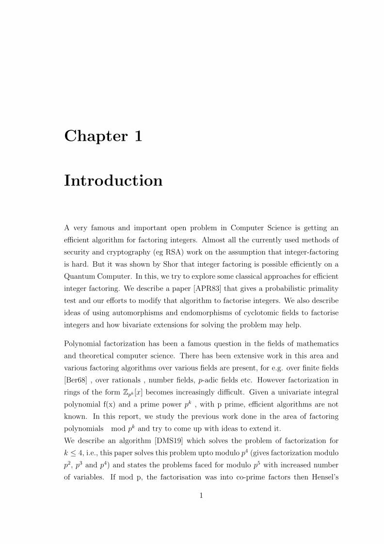
We describe an algorithm [DMS19] which solves the problem of factorization for
k ≤ 4, i.e., this paper solves this problem upto modulo p4 (gives factorization modulo
p2, p3 and p4) and states the problems faced for modulo p5 with increased number
of variables. If mod p, the factorisation was into co-prime factors then Hensel’s
1

Chapter 1: Introduction 2
lemma could have been used. So the only case that needs to be dealt with is when
f is power of an irreducible polynomial modulo p. This is solved by reducing this
problem to ”root finding” over some other idea. Our goal is to try to extend these
ideas to factorisation mod pk for k ≥ 5 We also give how our problem of factoring
polynomials mod pk related to extending the Hilbert’s Nullstellensatz problem.

Chapter 2
Preliminaries
2.1 Preliminaries
2.1.1 Representative Roots
Rings of the form Z/〈pk〉[x] for some prime p and integer k ≥ 1 are not unique fac-
torization domains and hence polynomials of degree d can have more than d roots
(infact exponentially many are possible). [JBQ13] devised a compact datastructure
for this to represent these exponentially many roots in polynomial space, which was
further used in [DMS19].
Representative roots are roots of a polynomial written in the form a + pi∗ which
means that all the roots have the form a + piy for every y ∈ Zpk−i−1 . The symbol
∗ represents the entire ring y ∈ Zpk−i−1 and a is a p-adic integer. This can be seen
as a compact datastructure to represent exponentially many values (exponential in
log p). For a in the form a0 + a1p + a2p2 + . . . ai−1p
i−1 for some aj’s ∈ Zp then we
have the set of representative roots as
Sa = {a0 + a1p+ a2p2 + . . . ai−1p
i−1 + y1pi + y2p
i+1 + · · ·+ yk−ipk−1|yj ∈ Zp}
We will consider ∗ as an entire ring, R and the following convention of writing will
be followed:
3
Chapter 2: Preliminaries 4
• u+ {∗} = {u+ ∗}, u{∗} = {u∗}∀u ∈ R
• c+ {a+ b∗} = {(a+ c) + b∗}, c{a+ b∗} = {ca+ cb∗}∀a, b, c ∈ R
2.1.2 Quotient Ideal
Given two ideals I and J of a commutative ring R, we define the quotient of I by J
as [DMS19],
I : J := {a ∈ R|aJ ⊂ I} (2.1)
Claim 1 (Cancellation): Suppose I is an ideal of ring R and a, b, c are three
elements in R. By definition of quotient ideals, ca ≡ cb mod I iff a ≡ b mod I : 〈c〉.Claim 2:Let p be a prime and φ ∈ (Z/〈pk〉)[x] be such that φ 6≡ 0 mod p. Given
an ideal I := 〈pl, φm〉of Z[x],
1.I : 〈pi〉 = 〈pl−i, φm〉, for i ≤ l, and
2.I : 〈φj〉 = 〈pl, φm−j〉 for j ≤ m.
Proof: We prove part 1. Part 2 is similar.If c ∈ 〈pl−i, φm〉 then there exists c1, c2 ∈Z[x], such that,c = c1p
li + c2φm. Multiplying by pi, we get pic = c1p
l + pic2φm =⇒
c ∈ I : 〈pi〉For reverse direction, suppose c ∈ I : 〈pi〉, then then there exists c1, c2 ∈ Z[x], such
that,pic = c1pl + c2φ
m. Since i ≤ l and p 6 |φ, pi|c2. So c = c1pl−i + ( c2
pi)φm =⇒ c ∈
〈pl−i, φm〉.
2.1.3 Gauss Quadratic Sums
Let p be an odd prime number and a an integer. Then the Gauss sum modulo p,
g(a; p) [Wiki], is the following sum of the pth roots of unity:
g(a; p) =
p−1∑n=0
e2πian2
p =
p−1∑n=0
ζan2
p , ζp = e2πip .
The exact value of the Gauss sum, computed by Gauss, is given by the formula
g(1; p) =
p−1∑n=0
e2πin2
p =
√p if p ≡ 1 (mod 4),
i√p if p ≡ 3 (mod 4).
Chapter 2: Preliminaries 5
g(1; p)2 =(−1p
)p was easy to prove and led to one of Gauss’s proofs of quadratic
reciprocity. However, the determination of the sign of the Gauss sum turned out to
be considerably more difficult and even Gauss could only establish it after several
years’ work.
2.1.4 B-near prime ideals
We define the concept of B-near prime ideals which are necessary for our algorithms
for power residue computation:
B-near prime numbers- A natural number N is said to be B-near prime if
N = p∏k
i=1 pi with pi ≤ B, p′is can be repeated.
B-near prime ideals-Ideal a of R is called B-near prime if its norm N(a) is B-near
prime.
Advantage of B-near prime ideals-They are efficiently recognisable and com-
putable in poly-time when B is polynomially bounded by the degree n=[K:Q]. Also,
their factorization can be computed efficiently.

Chapter 3
Integer Factoring-Previous work
We describe the main ideas from the paper [APR83] and how we tried to extend
these further. We will
The paper gives an algorithm for primality testing, which I will call APR algorithm
from now. We tried to modify it for factoring. Given n, the [APR83] algorithm
decides in time (logn)c log log log n (nearly polynomial time) whether it is prime or
composite. It works on principles of Power residue computations on cyclotomic
fields and consists of many pseudo-primality tests such that if n passes all the tests,
its factors lie in a small, explicit set.
3.1 Main Ideas of APR algorithm
Let I be a set of primes. A Euclidean prime with respect to I is a prime q such that
q-1 is sqaure free and every prime factor of q-1 lies in I. In the algorithm, we try
to find a small set of initial primes I=I(n) (={p1, p2, ...}) such that the product of
Euclidean primes( denoted by q1, q2, ...) exceeds√n.
Let tq be a primitive element of the field Fq. Then Indq(x) is the smallest non-
negative integer for which x = tIndq(x)q mod q
For a possible r (≤√n) dividing n, we want to find r mod q for each Euclidean
6

Chapter 3: Integer Factoring Ideas 7
prime q. As the product of these Euclidean primes is greater than r, we can get r
from the above using Chinese Remaindering. So we try to find Indq(r) for every
Euclidean prime q which would give us r mod q for each q.
For this, we try to calculate Indq(r) mod p for each initial prime p dividing q-1.Now
the size of the multiplicative group F ∗q is q-1. So by Chinese Remaindering would
give us Indq(r) mod (q-1) which is the same as Indq(r).
So our goal- Try to know Indq(r) mod p for each initial prime p dividing q-1. This
would give us r.
Transition data- For a fixed initial prime p, we find ”transition data” relating
Indq(r) mod p for all q such that p divides q-1 such that if one of them is known,
the others can be calculated in terms of it. The transition data is obtained by using
some ”mock residue symbols” (which are related to pth power residue symbols) and
”Extraction lemma”.
3.2 Tools used
Cyclotomic field of a prime p - Its irreducible polynomial over Q is φp(x) =
xp−1 + xp−2...x + 1 . We know φp(x) factorises mod q into equidegree irreducible
factors of degree f = order of q in (Z/pZ)*
The polynomial φp(x) factors mod q as φp(x) =∏g
i=1 hi(x) mod q where hi(x) are
distict monic polynomials of degree f which are irreducible mod q and g=p−1f
We now consider power residue symbols in the special case where q is a rational
prime and p — q-1. Let t = tq be a primitive root for q. Then
φp(x) =∏p−1
i=1 (x− t(q−1p
)i mod q ( here we use the fact that t(q−1p
) is a primitive pth
root of unity )
So we have ”canonical” prime Q lying over (q) in Z[ζp] as
Q = (q, ζp − t(q−1p
))
Now, ( xQ
)p
= xq−1p (Here size of Q is easily seen to be q)

Chapter 3: Integer Factoring Ideas 8
= tIndq(x)q−1p = ζ
Indq(x)p modQ
Thus knowing ( xQ
)p
for the canonical prime Q is equivalent to knowing Indq(x) mod
p, which was our goal.
Jacobi Sums: If Q is a prime of Q(ζp) not dividing (p) and a,b ∈ Z then the Jacobi
sum is defined as:
Ja,b(Q) =∑′
( xQ)
p−a( 1−xQ
)−bp
where the sum is over a set of coset representatives of
z[ζp]/Q other than 0,1 mod Q. The prime factorisation of (Ja,b(Q)) is given by the
following theorem
Theorem 3.1. [APR83] Suppose a,b ∈ Z with ab(a+b) 6= 0 mod p. For u ∈ Z, define
θ(u)a,b = [a+bpu]− [a
pu]− [ b
pu] (it is either 0 or 1), then
(Ja,b(Q)) =
p−1∏n=1
σ−1u (Q)θa,b(u)
Theorem 3.2. [APR83] If p > 2, there exist a, b in Z such that ab(a + b)6= 0 mod
p and we define
θa,b =
p−1∑u=1
θa,b(u).u−1 6= 0 mod p where u−1 is inverse of u mod p.
Proof: Note that for 1 < u < p - 1, we have [up] = 0 and [p−1
pu] = u− 1
Then
p−2∑m=1
θm,1 =
p−2∑m=1
p−1∑u=1
([m+ 1
pu]− [
m
pu]).u−1 =
p−1∑u=1
[p− 1
pu].u−1
=
p−1∑u=1
(u− 1).u−1 = p− 1 6= 0mod p
So there exists atleast one good pair (a,b) = (m,1) for m=1,2...p-2
3.3 Probablisitic Version of the APR Algorithm
3.3.1 Preparation
In the preparation step, we define the initial primes and calculate the transition
data. We first compute f(n), the least square-free natural number such that
Chapter 3: Integer Factoring Ideas 9
∏q−1|f(n),q∈primes
q > n12
We define initial primes for n to be the prime factors p of f(n) and the Euclidean
primes for n to be the primes q for which q − 1|f(n)
It is shown that f(n) ≤ (logn)co log log log n for all large n
Note it can be easily seen that the time taken to compute f(n) will be of the order
f(n)c . We then compute and fix a primitive root tq for each Euclidean prime q and
check that n is not divisible by p or q.For each initial prime p > 2, find a, b ∈ Z
such that 0 < a, b < p,
θa,b =
p−1∑u=1
θa,b(u).u−1 6= 0 mod p
Compute a ”Jacobi sum” Jp(q) for each initial prime p and Euclidean prime q with
p|q − 1 as follows:
If p = 2, put Jp(q) = −qIf p > 2, let Jp(q) = −Ja,b(Q) where a,b are from previous step
We have (Jp(q), r)λ=1
Then for each p,we factor n into ideals in Z[ζp] as it would happen if n was prime.
We attempt to do this as follows. Let f be the order of n in (Z/pZ)∗ , put g = (p -
1)/f, and try to factor φp(x) =∏g
i=1 hi(x) mod n
where each hi(x) ∈ Z[x] is monic and has degree f. If n is in fact prime, then with
high probability of success φp(x) can be so factored mod n using Berlekamp
3.3.2 Extraction
The mock residue symbol 〈 αQ〉p is defined as :
〈 αQ〉p = ζ ip ≡ α
NQ−1p mod Q if such a congruence holds
〈 αQ〉p= 0 otherwise
For each initial prime p and each Euclidean prime q with p|q − 1, compute the
mock residue symbols 〈Jp(q)Qi〉p for i=1..g for ideals Qi found during factorisation of
the previous section.. If any of the Mock Residue Symbols is 0, declare n to be
COMPOSITE.

Chapter 3: Integer Factoring Ideas 10
For each initial prime p, if the mock residue symbols for p are not all equal to
1, choose some nontrivial one, 〈γ/Q)p, and make it the distinguished symbol cor-
responding to the prime p. If they are all 1, we compute mock residue symbols
〈γ/Qi〉p for γ’s chosen at random in Z[ζp], until one is found to be not 0 or 1 and
designate it the distinguished symbol.
(The algorithm may diverge here, but if n is prime the probability of an arbitrarily
chosen γ working is roughly (p - 1)/p, so a very high probability)
For each pair p, q with p|(q − 1), compute the exponents mi,q such that
〈 γQ〉mi,qp = 〈Jp(q)
Qi〉p
Lemma 3.3. Extraction Lemma[APR83]
Let Q and Q1 be ideals of Z[ζp] such that p 6 |NQ = NQ1 and let R,R1 be conjugate
prime ideals dividing Q and Q1 respectively.
Suppose there is some γ ∈ Z[ζp] such that 〈 γQ〉p 6=0 or 1
Then 〈 γQ〉mp = 〈 α1
Q1〉p .................. (A)
implies ( γR
)mp = ( α1
R1)p ................. (B)
Proof : Let valuations vp(t) is defined as the largest integer k such that pk|t.Now the initial hypothesis is that γ
NQ−1p ≡ ζjp mod Q, j 6= 0 mod p
Reducing this to mod R we have, γNQ−1p ≡ ζjp mod R, j 6= 0 mod p
So we have vp(NR− 1) > vp(NQ−1p
) as NR− 1 is the order of (Z[ζp]/R)∗
First suppose R = R1. Then reducing the relation (A) mod R and using NR = NR1
we obtain
γNQ−1p m ≡ 〈 γ
Q〉mp = 〈 α1
Q1〉p = α
NQ−1p mod R
Let T be a primitive root of R. Then T (mInd(γ)−Ind(α)NQ−1p = 1 mod R. But order of
T is NR−1. So NR−1|(mInd(γ)−Ind(α)NQ−1p
. This implies p|(mInd(γ)−Ind(α)
from the first equation of the proof.
This in turn means the following is true (we replace Q with R in the previous equa-
tion)
T (mInd(γ)−Ind(α)NR−1p = 1 mod R
which gives γNR−1p m ≡ α
NR−1p mod R which is what we required (this is equation B).
The case in which R 6= R1 can easily be reduced to the above case and hence Ex-
traction lemma is also true in this case.

Chapter 3: Integer Factoring Ideas 11
The Extraction Lemma and the relations among the mock residue symbols allow
us to compute many power residue symbols in terms of one unknown one, via the
following calculation.
Suppose r is a prime number dividing n and p > 2 be an initial prime. Suppose 〈 γQ〉
is the distinguished symbol corresponding to p. Knowing this mock residue symbol
does not allow us to compute the power residue symbol (γ/(r,Q))p, but there are
only p possibilities for it.
Now (Jp(q)r
)p = ( rJp(q)
)p(Jp(q), r)λ = ( rJp(q)
)p
Now ( rJp(q)
)p =
p−1∏i=1
(r
σ−1u Q)θa,b(u)p =
p−1∏i=1
σ−1u (r
Q)θa,b(u)p ==
p−1∏i=1
(r
Q)u−1.θa,b(u)p = (
r
Q)θa,b(u)p
Also, (Jp(q)r
)p =
g∏i=1
(Jp(q)
r,Qi
)p =
g∏i=1
(γ
r,Q)mi,qp = (
γ
r,Q)∑gi=1mi,q
p
Now θa,b(u) is invertible. So (r
Q)p = (
γ
r,Q)θa,b(u)
−1∑gi=1mi,q
p
Thus if (γ
r,Q)p = ζkp then Indq(r) ≡ k.θa,b(u)−1
g∑i=1
mi,q mod p
This shows that the value of (γ/(r,Q))p completely determines each Indq(r) mod p
for every Euclidean prime q with p|q − 1. [APR83]
3.3.3 Consolidation step
Main Idea for consolidation is that if p1, ...pd are the initial primes and 〈 γiQi〉pi are
the corresponding distinguished symbols found in Preparation Step, then for each
prime factor r of n, there are integers k1, .., kd such that (γi
ri, Qi
)pi = ζkpi i for i=1...d
By the Chinese Remainder Theorem there is a single integer k defined modulo∏pi,
such that (γi
ri, Qi
)pi = ζkpi for i=1...d
For each k, 1 ≤ k ≤ f(n) =∏pi, we assemble and test a possible divisor r= r(k) of
n.
Check whether r(k)|n. If it does and r(k) 6= 1 or n, declare n composite and halt.
Otherwise continue with the next value of k. If none of these divide, we declare n
to be prime. For if n is composite it must have a prime factor r ≤ n12

Chapter 3: Integer Factoring Ideas 12
3.4 Ideas for Calculating the Power residue sym-
bol efficiently
The idea of calculating the power residue symbol efficiently was introduced in
[dBP17]. We briefly describe the algorithm that they introduced in which (αb)m
is calculated in 3 stages:
• Principalization- Reducing computation of (αb)m
to (αβ)m
for some β ∈ b
• Reduction(Optional)- Reduce computation of (αβ)m
for large α, β ∈ K to (αiβi
)m
fo smaller αi, βi ∈ K
• Evaluation-Computing (αiβi
)m
directly using prime density results
3.4.1 Principalisation Algorithm:
The main idea used here is to use random sampling relatively small elements to get
a B-prime ideal which can be efficiently factorized. Then using this previous fac-
torization and the reciprocity of residue symbols, we can reduce the power residue
computation to a simpler power residue computation.
3.4.2 Evaluation Algorithm:
Power Residue(αo, β)
Note:(αiγm
β)m
= (αiβ
)m
This property is used here
The idea behind evaluation is to repeatedly choose a random γ and set α = αoγm
until α mod β has a small representative α that generates a B near-prime ideal.
We then use reciprocity to reduce (α0
β)m
to calculation of U(αo, β) and (βα
)m
(which
can be done by the factorisation of B-near prime ideals).

Chapter 3: Integer Factoring Ideas 13
3.4.3 Reduction
- This is optional. Usually done when in (αβ)m
either one(case A) or both (case B)of
α, β are large.
In case A, assume α is much larger than β. Here compute LLL-reduced basis Mβ of
ideal (β) and reduce α mod Mβ. The reduced α is hoped to have similar size as β.
In case B, both inputs are large, say with bitsize g(n)>6n where n=[K:Q]. Consider
the lattice L={(γ1, γ2) ∈ OK x OK |γ1a − γ2 ∈ (β) }. This lattice has discriminant
N(β) and dimension 2n. Applying LLL, we get a short vector (γ1, γ2) ∈ O2Kwith√
||γ1||2 + ||γ2||2 ≤ 2nN(β)12n ≈ 2n||β|| 12 ≈ 2
g(n)+2n3 ≤ 2
2g(n)3 ≈ ||β|| 23
where it is assumed heuristically that ||β|| ≈ N(β)1n and ||β|| ≈ 2g(n)
Now γ1α = kβ + γ2 So we can write (γ1β
)m
(αβ)m
= (γ2β
)m
Or (αβ)m
= (γ2β
)m
(γ1β
)−1m
.
So computation of power residue symbol is reduced to computation of 2 power
residue symbols with smaller imput. This process can be some repeatedly to reduce
the size of input forming a recursion tree.
This gives us an efficient method of calculating the power residue symbols.

Chapter 4
Integer Factoring-New Ideas
4.1 Extension of APR ideas for factoring integers
We know from the paper that transition data is obtained by using some ”mock
residue symbols” (which are related to pth power residue symbols) and ”Extraction
lemma”. We tried to replace the use of ”mock residue” symbols by actual residue
symbols which can be computed using the ideas of the previous section. But we saw
that the particular form of mock residue symbols is essential for the extraction lemma
to work which wont be possible with actual residue symbols. So the ”Extraction
lemma” in its current form can’t be used with actual residue symbols. So we tried
some modifications to the extraction lemma but they were not efficient.
Now the APR algorithm works on the following idea:
if our number (n=rr’ for prime r, r′) was passing all pseudo primality tests, it gives
an explicit factor of n (ie, r or r’). Passing the pseudo primality tests would depend
on the initial primes we take. So we try to select a ”good” set of initial primes such
that the pseudo-primality tests are passed .
Another thing we claim from the extraction lemma is that in APR algorithm, with
high probability, none of the mock residue symbols would be 0 ( and hence the
algorithms tries to find an explicit factor of n=rr’) if the behaviour of r and r is
indistinguishable in terms of the mock-residue symbols. So our claim was that if
ordp(r)|ordp(n) and ordp(r′)|ordp(n) for all the initial primes p, we would be able to
14

Chapter 4: Integer Factoring- New Ideas 15
factorise n. Basically, if n=rr’ (for distinct primes r,r’) then we clain that factoring
would succeed as long as their algorithm steps are ”identical mod r and mod r’ ”.
So our idea is we start with lots of initial primes p, and form lots of Euclidean primes
q and find a ”good” set of primes such that the behaviour of APR mod r and mod r’
is same, and then run the APR-algo for this set which should factorize n. But doing
this using brute force would lead to a huge time complexity which would make our
algorithm inefficient. Thus we need to think of a clever way of selecting the initial
primes.
4.2 Factoring n=pq using ideas of Automorphisms
in Cyclotomic Fields
Let R = (Z/nZ). By Chinese remaindering, we see that R∼= (Z/pZ) x (Z/qZ).
Now as p and q are primes, we see that (Z/pZ) and (Z/qZ) are fields. Now we
want cyclotomic extensions of these fields. So we work in R/(φr(x)) where φr(x) =
xr−1 + xr−2...x + 1 for some prime r. Again by Chinese remaindering, we see that
R/(φr(x))∼= (Z/pZ)/(φr(x)) x (Z/qZ)/(φr(x)) . Thus we see that the ring in
which we work can be seen as the product of two cyclotomic extensions of a field.
(Z/pZ)/(φr(x)) can also be represented by Fp(ζr). The intuitive reason for this
is that in this cyclotomic extension of Fp, powers of x are the r-th roots of the
polynomial xr − 1. Hence x can be thought of as ζr, ie, the r-th primitive root of
unity.
First we see what kind of automorphisms can be present in a cyclotomic extension:
σ ∈ Aut(Fp(zetar)) iff σ : ζr 7→ ζ ir for some i coprime to r. The reason for this is
that any automorphism σ can only map ζr to another root. ( This can also be seen
using the Frobenius automorphism. Any automorphism σ : ζr 7→ ζpi
r which gives
the same set of automorphisms as above ). This gives that the only automorphisms
possible in this cyclotomic extensions are x 7→ xi
Chapter 4: Integer Factoring- New Ideas 16
Claim- If we get any map φ in (Z/nZ)/(φr(x)) that is an automorphism in one of
the decomposed cyclotomic fields/rings but not in the other , then we will be able
to factor n = pq
The reason is that since φ is an automorphism in only one of the cyclotomic extension
( WLOG, say (Z/pZ)/(φr(x))) but not in the other field, we see that:
φ(ab)− φ(a)φ(b) would be zero mod p but not not q.
So we can take gcd(n,φ(ab)− φ(a)φ(b)) to get p and hence factorise n=pq.
Also we see that any such map φ would be different from x 7→ xi. So our aim is
to find a map φ different from x 7→ xi that is an automorphism in the decomposed
field. (We can also see that if such a map exists using counting argument. Also if
we are able to find such a map, another way to factor n would be to take the gcd of
the coefficients with n, as atleast some coefficient would have a non-trivial gcd with
n in this case).
We tried to use interpolation ideas to set up equations to find such an automorphism
(different from xi). Idea- set-up eqns like a(x) = x2, a(x6) = x4 and their swaps and
then get the resultant polynomial using interpolation and see if it behaves as an
automorphism. But on checking carefully, we saw that the interpolation idea in
univariate field extension is problematic, as you don’t have access to ζ. We only
have ’x’ and even though x can be thought of as the r-th root of unity, it behaviour
is different from that of ζ.
For eg., suppose we have r=7 such that we have ζ7 = 1 and we set up an equation
a(x) = x2, a(x6) = x4. Then a(ζ) = ζ2 ⇒ a(ζ6) = ζ12 = ζ5 6= ζ4. so the two eqns
are inconsistent. So our goal is that somehow we need BOTH ζ and x to play this
strategy. We think that bivariate extension of the field should help in this case and
we are currently exploring these.
Using python code, we also tried to see the pattern that the Frobenius morphism
gives in the decomposed field such that we are able to find an algorithm for inter-
polation. We took particular value of p. I took p=13 = -1 mod 7 so that we get
(F 2p )3.Here(x7 − 1)/(x− 1) = (x2 + 3x+ 1)(x2 + 5x+ 1)(x2 + 6x+ 1).
Objective: To find an a(x) other than xi which gives an automorphism

Chapter 4: Integer Factoring- New Ideas 17
A pattern we noticed was this: For a(x) = xi in the original ring, x 7→ xi in the
decomposed fields too but it also can introduce swaps.
In simple words, say I get an element e=(3x, x, 0) (these components are using
Chinese remaindering). Then with a(x) = x2, e maps to (0, 3x2, x2) and with a(x) =
x3, e maps to (x3, 0, 3x3) and so on. So we think that to get a φ(x)other than xi, we
need to find a map such that (x, x, x) maps to say (x, x2, x) Instead of say (x2, x2, x2)
or something similar. This gives us insight into what kind of automorphisms in the
decomposed field can help.
4.3 Factoring n=pq using Gauss Quadratic sums
We had the following idea for factorizing n=pq using Gauss sums. We know that
for an odd number p g(1; p)2 =(−1p
)p. The idea is to pick a random prime s.
Define r = s2 such that φr is irreducible mod p and mod q. We know that with high
probability this would be true.
Also s2 = 1 mod 4, so r = 1 mod 4. Now we compute the gauss sum g(1;r)
in the ring R = (Z/nZ)(ζr) = (Z/nZ)[x]/(φr(x)) where φr is the r-th cyclotomic
polynomial. So g(1; r) =√
(s2) = s or −s. Also with high probability, we can
assume that p and q have different quadratic residuositues mod r. WLOG assume
that (p/r)=1 and (q/r)=-1. Then we compute the gcd(g-s,n). Then we know that
as g =√r, we claimed that with high probability g = s mod p but g 6= s mod q
due to our quadratic residuosity assumptions. So the gcd (g-s, n) should give us a
non-trivial factor of n=pq. ANother way would be see the coefficients of g to get a
factor
So our algorithm was as follows:
•• Input n=p.q. Randomly pick prime r =1 mod 4. [r= polylog(n)]
• By Gauss theorem: g2 = r. Here g is the Gauss Quadratic sum.
• With high probability (r/p)=(p/r)=1 AND (r/q)=(q/r)=-1.
• By (1) and cyclotomic-ring: g(x)2 = r mod 〈p, φr(x)〉. By (2) : g(x) ∈ Fp.
• By (1) and cyclotomic-ring: g(x)2 = rmod〈q, φr(x)〉. By (2): g(x) /∈ Fq.
Chapter 4: Integer Factoring- New Ideas 18
• By (3)-(4): g(x) mod 〈n, φr(x)〉 written in reduced form, has some coefficient
that factors n, by gcd.
We wrote a code for this and saw that the algorithm was not giving the gcd correctly
and hence not factoring n. The reason we saw for this is that g(x) ∈ Fp was not
coming out to be true. It was not giving a number. The reason for this was as follows,
we know that as (r/p)=(p/r)=1, φr(x) mod p has atleast 2 factors (say f1 . . . fk) as
the number of factors are even. Then for g(x) to be a number mod 〈p, φr(x)〉, we
would need g(x) mod fi to all give the same sign (ie, the Gauss sum should give
the same sign in the decomposed field’s). But we saw that the signs were not all
same. Instead half of these gave + signs and half of these gave - signs which led to g
not being a number mod 〈p, φr(x)〉. This creates a problem so that our algorithm
cannot factorise n=pq.

Chapter 5
Polynomial Factoring
Ideas-Previous Work
We first present previous work done in this and our efforts to extend it. We present
a report of[DMS19]. The main idea in this paper for factorization modulo pk for
some prime k is by using ROOT-FIND algorithm introduced in [JBQ13] and further
modified in [DMS19]. For the polynomial factoring into coprime factors modulo p
it can be easily lifted using Hensel Lifting [BS66] to modulo pk for any k. So we
consider only the hard case when f(x) mod p is a perfect power of some irreducible,
i.e. f(x) ≡ φe mod p for an irreducible polynomial φ(x) ∈ Z[x]. The given method
works on factorizing it in the ring (Z/pkZ)[x] by reducing it to root-finding of a
bivariate polynomial E(y), with coefficients of y in Z[x], in the ring (Z[x]/〈pk, φak〉)[y]
for some a ≤ e.
Theorem 5.1. [DMS19] Given a prime p, k ≤ 4 and a univariate polynomial f(x)
with integral coefficients. Then f(x) mod pk can be efficiently factored and tested
for irreducibility in randomized poly(deg(f), log p) time.
Theorem 5.2. [DMS19] Given a prime p, an integer k ≤ 4 and a univariate poly-
nomial f(x) which is the power of an irreducible modulo p and g is a factor of f mod
p, we can count all the factors g (which are lifts of g) of f mod pk (or decide that
it is irreducible) and represent them in a compact datastructure.
19

Chapter 5: Polynomial Factoring Ideas-Previous Work 20
Proof idea for Theorem 5.1: We only consider the hard case, ie, assume that f(x),
of degree d satisfies f(x) ≡ φ(x)e mod p for some irreducible integral polynomial φ
and deg(φ)e ≤ d. Otherwise we can easily use Hensel’s lifting to find a factorization.
So we have f of the form φe + pf ′ for some polynomial f ′(x) ∈ (Z/〈pk〉)[x]. The
factors of f will be of the form φa−py for y ∈ (Z/〈pk〉)[x]. The idea of this approach
is so divide f(x) by h(x) and binomially expand 11−x = 1 + x + x2 + x3 + . . . and
using this, we can reduce the problem of factorization to that of root finding in
bigenerated ideal which in the case of p4 can be efficiently found.
Proof idea for Theorem 5.2: We want to find, for each a < e, polynomials of the
form g(x) ≡ φa mod p such that it lifts to modulo pk and divides f in Zpk . For a
fixed a we can find all y’s modulo pk−1 from the proof of theorem 1, which can be
obtained from the modification to the root find algorithm. Then we can sum over
all the a’s for which it lifts.
5.1 Main Results
5.1.1 Reduction of Factoring to Root-Finding
In this subsection, we describe a polynomial E(y) which will help in finding a factor
of f ≡ φe + pl mod pk which is h ≡ φa− py mod pk where a ≤ e/2. This is true as
if g is a polynomial such that f ≡ gh mod pk, then looking modulo p we will have
exactly one of them contributing to the power of φ less than or equal to e/2. We
choose this factor as h.
Throughout the rest of this report we denote Z[x]/〈pk, φak〉 as R and Z[x]/〈p, φak〉as R0. Now we define the polynomial E(y) ∈ R[y] as
E(y) = f(x)(φa(k−1) + φa(k−2)py + φa(k−3)(py)2 + · · ·+ φ(py)k−2 + (py)k−1) (5.1)
We now reduce the factoring f(x) modulo pk to root-finding of E(y) modulo the
bi-generated ideal 〈pk, φak〉.

Chapter 5: Polynomial Factoring Ideas-Previous Work 21
Theorem 5.3. Reduction Theorem[DMS19]
Given two polynomials f(x) ≡ φe + pl mod pk and h(x) ≡ φa − py mod pk for
a ≤ e, we will have h(x) as a factor of f(x) if and only if E(y) ≡ 0 mod 〈pk, φak〉(i.e. y is a root of E(y) in R), for notations as defined above.
Now if we denote y = y0 + py1 + p2y2 + . . . pk−1yk−1, the next lemma reduces the
precision of y.
Lemma 5.4. [DMS19] If y = y0 + py1 + p2y2 + . . . pk−1yk−1, then every element of
the set y0 + py1 + . . . pk−3yk−3 + pk−2∗ is a root of E(y) modulo 〈pk, φak〉.Proof: Notice that in the expansion of E(y) all the y’s that are present are multiplied
by p, which implies yk−1 will have coefficient divisible by pk, which is 0 in R. Also
for yk−2, all the terms of the form (py)i for i ≥ 2 do not contribute as they are
zero in R. The only remaining term is f(x)φa(k−2)py. Now f(x)φa(k−2) ≡ φe+ak−2a
mod 〈p, φak〉 which also vanishes modulo 〈pk, φak〉, as e ≥ 2a.
Next we can have this following modification of the root-find algorithm discovered
in[JBQ13]. This modification in due to [DMS19]
Theorem 5.5. [DMS19] Given a bivariate polynomial g(y) ∈ R0[y], let Z ⊂ R0 be
the root set of g(y). Then Z can be written as the disjoint union of atmost degy(g(y))
many representative pairs (a0, i0), a0 ∈ R0, i0 ∈ R0. These representative roots can
be found in randomized poly- time.
For the next subsection and the rest of the report we fix k = 4. Similar techniques
can be applied for k = 2, 3 as well.
Chapter 5: Polynomial Factoring Ideas-Previous Work 22
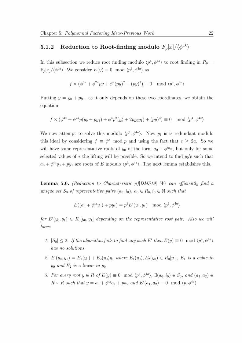
5.1.2 Reduction to Root-finding modulo Fp[x]/〈φak〉
In this subsection we reduce root finding modulo 〈p4, φ4a〉 to root finding in R0 =
Fp[x]/〈φ4a〉. We consider E(y) ≡ 0 mod 〈p4, φ4a〉 as
f × (φ3a + φ2apy + φa(py)2 + (py)3) ≡ 0 mod 〈p4, φ4a〉
Putting y = y0 + py1, as it only depends on these two coordinates, we obtain the
equation
f × (φ3a + φ2ap(y0 + py1) + φap2(y20 + 2py0y1) + (py)3) ≡ 0 mod 〈p4, φ4a〉
We now attempt to solve this modulo 〈p3, φ4a〉. Now y1 is is redundant modulo
this ideal by considering f ≡ φe mod p and using the fact that e ≥ 2a. So we
will have some representative roots of y0 of the form a0 + φi0∗, but only for some
selected values of ∗ the lifting will be possible. So we intend to find y0’s such that
a0 + φi0y0 + py1 are roots of E modulo 〈p3, φ4a〉. The next lemma establishes this.
Lemma 5.6. (Reduction to Characteristic p)[DMS19] We can efficiently find a
unique set S0 of representative pairs (a0, i0), a0 ∈ R0, i0 ∈ N such that
E((a0 + φi0y0) + py1) = p3E ′(y0, y1) mod 〈p4, φ4a〉
for E ′(y0, y1) ∈ R0[y0, y1] depending on the representative root pair. Also we will
have:
1. |S0| ≤ 2. If the algorithm fails to find any such E ′ then E(y) ≡ 0 mod 〈p4, φ4a〉has no solutions
2. E ′(y0, y1) = E1(y0) + E2(y0)y1 where E1(y0), E2(y0) ∈ R0[y0], E1 is a cubic in
y0 and E2 is a linear in y0
3. For every root y ∈ R of E(y) ≡ 0 mod 〈p4, φ4a〉, ∃(a0, i0) ∈ S0, and (a1, a2) ∈R×R such that y = a0 + φi0a1 + pa2 and E ′(a1, a2) ≡ 0 mod 〈p, φ4a〉
Chapter 5: Polynomial Factoring Ideas-Previous Work 23
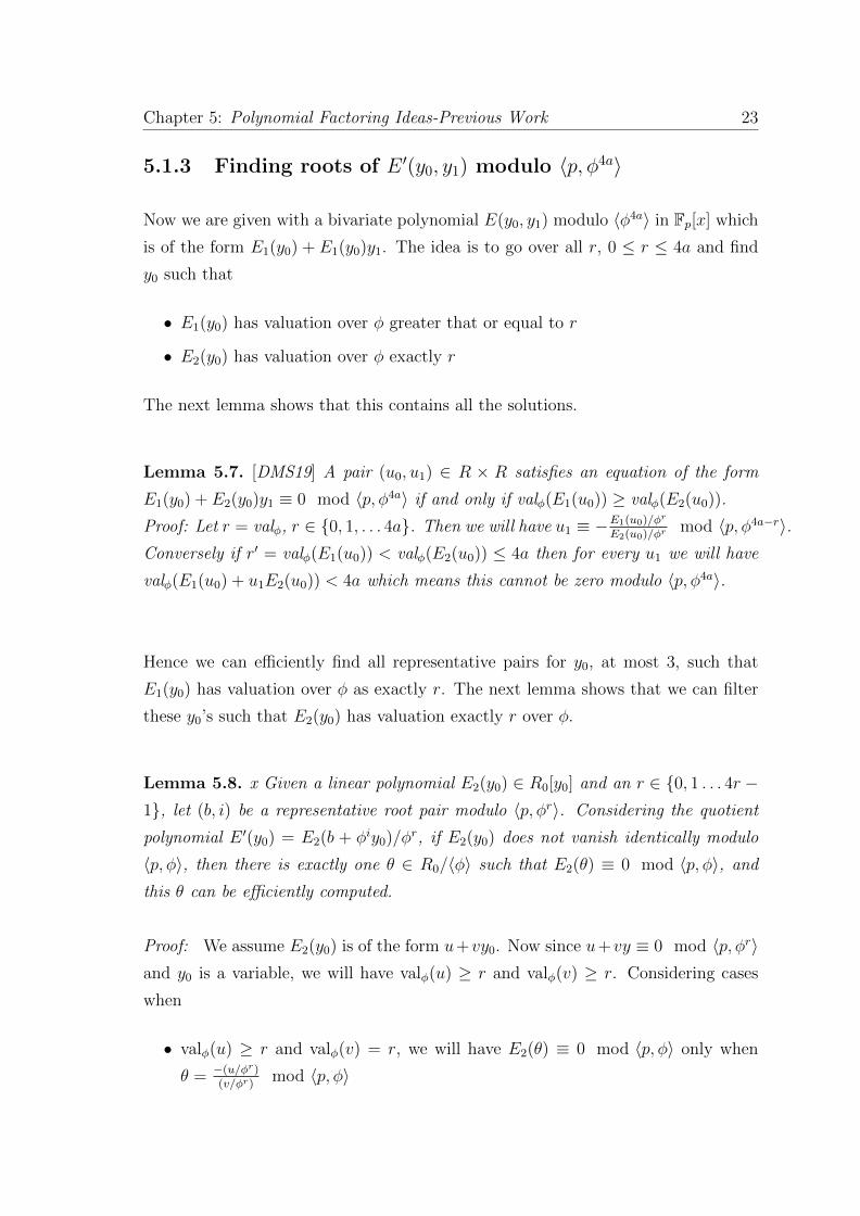
5.1.3 Finding roots of E ′(y0, y1) modulo 〈p, φ4a〉
Now we are given with a bivariate polynomial E(y0, y1) modulo 〈φ4a〉 in Fp[x] which
is of the form E1(y0) + E1(y0)y1. The idea is to go over all r, 0 ≤ r ≤ 4a and find
y0 such that
• E1(y0) has valuation over φ greater that or equal to r
• E2(y0) has valuation over φ exactly r
The next lemma shows that this contains all the solutions.
Lemma 5.7. [DMS19] A pair (u0, u1) ∈ R × R satisfies an equation of the form
E1(y0) + E2(y0)y1 ≡ 0 mod 〈p, φ4a〉 if and only if valφ(E1(u0)) ≥ valφ(E2(u0)).
Proof: Let r = valφ, r ∈ {0, 1, . . . 4a}. Then we will have u1 ≡ −E1(u0)/φr
E2(u0)/φrmod 〈p, φ4a−r〉.
Conversely if r′ = valφ(E1(u0)) < valφ(E2(u0)) ≤ 4a then for every u1 we will have
valφ(E1(u0) + u1E2(u0)) < 4a which means this cannot be zero modulo 〈p, φ4a〉.
Hence we can efficiently find all representative pairs for y0, at most 3, such that
E1(y0) has valuation over φ as exactly r. The next lemma shows that we can filter
these y0’s such that E2(y0) has valuation exactly r over φ.
Lemma 5.8. x Given a linear polynomial E2(y0) ∈ R0[y0] and an r ∈ {0, 1 . . . 4r −1}, let (b, i) be a representative root pair modulo 〈p, φr〉. Considering the quotient
polynomial E ′(y0) = E2(b + φiy0)/φr, if E2(y0) does not vanish identically modulo
〈p, φ〉, then there is exactly one θ ∈ R0/〈φ〉 such that E2(θ) ≡ 0 mod 〈p, φ〉, and
this θ can be efficiently computed.
Proof: We assume E2(y0) is of the form u+vy0. Now since u+vy ≡ 0 mod 〈p, φr〉and y0 is a variable, we will have valφ(u) ≥ r and valφ(v) ≥ r. Considering cases
when
• valφ(u) ≥ r and valφ(v) = r, we will have E2(θ) ≡ 0 mod 〈p, φ〉 only when
θ = −(u/φr)(v/φr)
mod 〈p, φ〉

Chapter 5: Polynomial Factoring Ideas-Previous Work 24
• valφ(u) = r and valφ(v) > r, E2(θ) will not be zero modulo 〈p, φ〉 for any θ in
R0/〈φ〉
• valφ(u) > r and valφ(v) > r, then we will have some greater value of r.
Thus in this way θ can be efficiently computed.
5.1.4 Algorithm to find Roots of E(y)
With these aforementioned lemmas and theorems we present the algorithm to find
roots of E(y) modulo 〈p4, φ4a〉 of Z[x][DMS19]
Theorem 5.9. [DMS19] The output of Algorithm 1 (set Z - Z0 ) contains exactly
those y0 ∈ R0 for which there exist some y1 ∈ R0, such that, y = y0 + py1 is a root

Chapter 5: Polynomial Factoring Ideas-Previous Work 25
of E(y) in R. We can easily compute the set of y1 corresponding to a given y0 ∈ Z- Z0 in poly(deg f, log p) time. Thus, we efficiently describe (and exactly count) the
roots y = y0 + py1 + p2y2 in R of E(y), where y0, y1 ∈ R0 are as above and y2 can
assume any value from R.
5.2 Wrapping up the theorems
5.2.1 Theorem 5.1
The only non trivial case is when f is a power of an irreducible mod p. In this case,
we can assume φa − py is a factor of f(x) and use Algo 1 to check if this is possible
or not. We do this for all a ≤ e2
and hence is a polytime algorithm.
5.2.2 Theorem 5.2
As g is a factor of f mod p, we know g = vφ(x)a where v is a unit. Any lift of this to
mod p4 is of the form g(x) = v(x)(φ(x)a − py) mod p4 for a unit v(x) ∈ (v + p∗) ⊂(Z/〈p4〉)[x]. Any such g(x) maps uniquely to g1(x) = v(x)−1g = (φ(x)a − py)
mod p4. So we only need to consider lifts of φ(x)a mod p
Now any lift of φ(x)a mod p which is a factor of f is of the form φ(x)a − py(x)
mod p4 for a polynomial y(x) ∈ (Z/〈p4〉)[x]. From the previous discussion, this can
be done in poly time using root finding in a different ring (using previous reductions)
for all a ≤ e/2
For a > e/2 replace b := e− a ≤ e/2 which can be solved as before.
Chapter 6
Polynomial Factoring-New Ideas
We describe some efforts made by us during this project to extend the existing
results for factorising and the problems that we faced.
6.1 Using Multivariate Representative Roots
Claim: If we can generate representative roots mod 〈xl, pk〉 , then we could induc-
tively extend this process inductively from k to k+1.
Proof: Our aim is to find roots mod 〈xl, pk〉 of a given polynomial g . We know we
can find representative roots mod 〈xl, p〉 from before. Let the representative root
that we get be r. (we treat this representative root as a multivariate)
So we can write g(r) = α.xl + β.p Here α, β are polynomials in multiple variables.
Now we want this to be 0 mod 〈xl, pk〉 . So this reduces to finding roots of β mod
〈xl, pk−1〉
This method works well for the extending k=1 to k=2. But for higher k’s (say
k=3), we would need representative roots of multivariates mod 〈xl, p〉. Now finding
a single root of such an equation over multivariate is possible but there is no such
known method for finding multivariate representative roots in the previous case. So
this is where this idea fails.
26

Chapter 6: Polynomial Factoring-New Ideas 27
For eg. an elliptic curve y2 = x3 + 1 mod p, we can easily find a ”root”... but no
efficient algorithm (or even representation is known for multivariate case. In fact in
this case, it seems that there are just way too many isolated roots to list (each root
roots seems its own representative).
Our aim is to find an efficient representation and algorithm for finding representative
roots in the multivariate case.
Another thing that we explored was trying to reduce powers of x in the previous
idea as compared to powers of p.
6.2 Relation to HN
We tried to extend the previous idea of treating the representative roots as multi-
variates to the following. We tried to think of representative root as:
Representative root r :=∑
i,j uij.xi.pj; where uij belong to the field Fp. Now we
to tried set g(r) = 0 mod 〈pk, xl〉 to get a variety in constant-vars. This we thought
could be solved using HN ideas.
So we considered the following algorithm:
• We need (φa − pY ) dividing f(x) mod 〈pk, φ(x)l〉; where (f = φe mod p).
• Using this reduction we first find E(Y) (as done previously using binomial
expansion); then we directly get the variety from: E(∑
ij Yij.pi.φ(x)j) = 0
mod 〈pk, φ(x)l〉. (the variety is obtained by comparing the coefficients of powers
of x, the RHS has all of them as 0)
• This variety is in vars Yij. You want these roots in the finite field Fp[z]/〈phi(z)〉.
• Use Hilbert’s Nullstellensatz related ideal computations to test whether this
ideal is empty.
However we noticed that HN reduction is faulty. For eg., from a0 +p.a1 = 0 mod p2
we can deduce: a0 = 0 mod p and a0/p+ a1 = 0 mod p. But we can’t say: a1 = 0
mod p. This stops simple reduction from HN mod pk to HN mod p. Hence factoring

Chapter 6: Polynomial Factoring-New Ideas 28
deg=4 polynomial f(x) mod p2 using this idea of reduction to HN in poly(log p)-time
is open.
In simple terms, the problem is that when we try to reduce the HN mod pk to HN
mod p , we do not get a single instance of HN mod p but a large (exponential)
number of possibile instances for HN mod p which can’t be solved efficiently. We
are considering ideas from algebraic geometry to solve these.
So we see that if we are able to solve HN mod pk efficiently, we will be able to factor
polynomials mod pk efficiently for any k which is our goal (and an open question
right now).

Bibliography
[APR83] Leonard M. Adleman, Carl Pomerance, and S. Robert. On distinguishing
prime numbers from composite numbers. Annals of Mathematics, 1983.
[Ber68] Elwyn R Berlekamp. Factoring polynomials over finite fields. Algebraic
Coding Theory., 1968.
[dBP17] Koen de Boer and Carlo Pagano. Calculating the power residue symbol
and ibeta. ISSAC, 2017.
[DMS19] Ashish Dwivedi, Rajat Mittal, and Nitin Saxena. Efficiently factoring
polynomials modulo p4. ISSAC, 2019.
[JBQ13] Gregoire Lecerf Jeremy Berthomieu and Guillaume Quintin. Polynomial
root finding over local rings and application to error correcting codes.
Applicable Algebra in Engineering, Communication and Computing,, 2013.
29


![An Improved Multivariate Polynomial Factoring Algorithm...factoring algorithm. A comparison with Musser's factoring algorithm [11] is presented. Being interested in heuristic factoring](https://cdn.vdocuments.us/doc/165x107/600bdf2763b48218ec7032be/an-improved-multivariate-polynomial-factoring-factoring-algorithm-a-comparison.jpg)


