
Infrastructure Investment in Europeand International Competitiveness
Debora Revoltella, EIBPhilipp-Bastian Brutscher, EIB
Alexandra Tsiotras, EIB ConsultantC. Weiss, EIB
EIB Working Papers 2016 / 01


1
Infrastructure Investment in Europe and International Competitiveness1
DEBORA REVOLTELLA, PHILIPP-BASTIAN BRUTSCHER, ALEXANDRA TSIOTRAS, CHRISTOPH WEISS 2
Summary
Infrastructure investment in Europe has been adversely affected by the economic crisis,
undermining both the immediate recovery and longer-term growth potential. This paper
discusses recent trends in infrastructure investment and finance in Europe, before exploring
one way in which transport infrastructure – the sector that has been arguably hardest hit by
the crisis – contributes to regional growth. Using a novel approach, we show that firms in
regions with a more developed transport network are better placed to benefit from positive
growth opportunities than firms in regions with a lower transport stock. This advantage is
most pronounced in times of economic stress – making a good transport infrastructure a key
ingredient for economic recovery. This indicates one channel through which the activities of
the European Investment Bank, now extended through the Investment Plan for Europe, can be
expected to foster growth and enhance competitiveness in Europe.
1. Introduction
An adequate supply of infrastructure is an essential ingredient for competitiveness and long
run potential growth in an economy. The public and private stock of infrastructure plays a
critical role in enhancing the productivity of people and firms throughout the economy by
lowering the costs of combining different productive inputs, accessing markets and by
increasing mobility and competition. Achieving and maintaining efficient infrastructure in the
education, energy, health, ICT, transport, water and waste sectors depends on sustained long-
term investment.
Investment in infrastructure has received heightened attention in Europe in recent years. In
particular, the marked retrenchment of both the public and private sector from their
infrastructure investment activities with the onset of the Euro crisis has spurred wide-spread
concern of the negative consequences this might have. Indeed, this crisis-related retrenchment
1 Disclaimer: The views expressed are those of the authors and do not necessarily reflect the position of the EIB. 2 We thank Tim Bending and Pedro de Lima for useful discussion. The views expressed in this paper are those of the authors and do not reflect those of the EIB. All errors are our own.

2
can be seen as merely compounding longstanding under-investment in critical infrastructure
in Europe.
To put recent crisis-related trends in context, it is possible to compare current levels of
infrastructure investment in the EU with approximate estimates of annual investment needs
with regard to both the replacement of assets reaching the end of their economic life and to
the achievement of key European policy goals.
For example, recent estimates find that investment will need to increase by 50% over 2014
levels in order to meet policy goals in the modernisation of urban transport and ensuring
sufficient capacity in inter-urban transport, which will facilitate growing trade and further
integration of the EU’s internal market. Taking also into account the need to address the
crisis-related backlog, this corresponds to extra investment flows of approximately EUR 50bn
per year.3
In the energy sector, it is estimated that achieving policy goals in terms of upgrading energy
networks to integrate renewables and ensure security of supply, increasing power generation
from renewables and energy efficiency in buildings and industry will require additional
annual invest in the order of EUR 100bn.4 Meanwhile achieving the EU’s Digital Agenda
targets and matching US data centre capacity is expected to require additional annual
investment of approximately EUR 55bn.5 Further large annual investment shortfalls can be
identified for sectors such as water and flood management as well as waste management and
materials recovery.
It is in the context of these structural investment gaps that the Investment Plan for Europe has
been launched. As a pillar of the plan, the European Fund for Strategic Investment (EFSI) has
been designed to provide an impulse for up to EUR 315bn of new investment over three
years, mostly from the private sector, with three quarters of the fund focused on innovation
and infrastructure.
This paper begins by providing an overview of recent trends in infrastructure investment in
Europe, with regard to sectors, geographical regions and sources of finance, including project
financing. We also discuss some of the current key constraints on infrastructure investment.
3 EIB estimates for 2015-2020 based on OECD/ITF statistics (accessed February 2014). 4 European Commission estimates of average annual investment in EU-28 over the period 2016 to 2030, supplemented on by EIB estimates. The scenario assumes compliance with all existing EU legislation, plus adoption of a 40% GHG target by 2030. See also Berndt et al. (2015). 5 EIB estimates for 2014 to 2020. See also Hätönen, J. (2011) and WEF (2011).

3
We then turn to focus in greater depth on the importance of infrastructure investment for
competitiveness and growth, using the transport sector as an example. We find that a well-
developed transport infrastructure stock is instrumental when it comes to linking local
businesses with their global growth opportunities. We show that firms in regions with a more
developed transport network are better placed to benefit from positive growth opportunities
than firms in regions with a less well developed transport stock. This advantage is most
pronounced in times of economic stress – making a good transport infrastructure a key
ingredient for economic recovery.
The last section is a conclusion of this analysis in connection with the role of the EIB and the
Investment Plan for Europe.
2. Evolution of Infrastructure Investment in the EU
This section provides an update of the state of infrastructure investment in Europe, by year,
sector and source of finance. Data on infrastructure investment, let alone its financing sources,
are not available in any ready-to-use form. We follow Wagenvoort et al. (2010) to compute
workable estimates of infrastructure investment.6
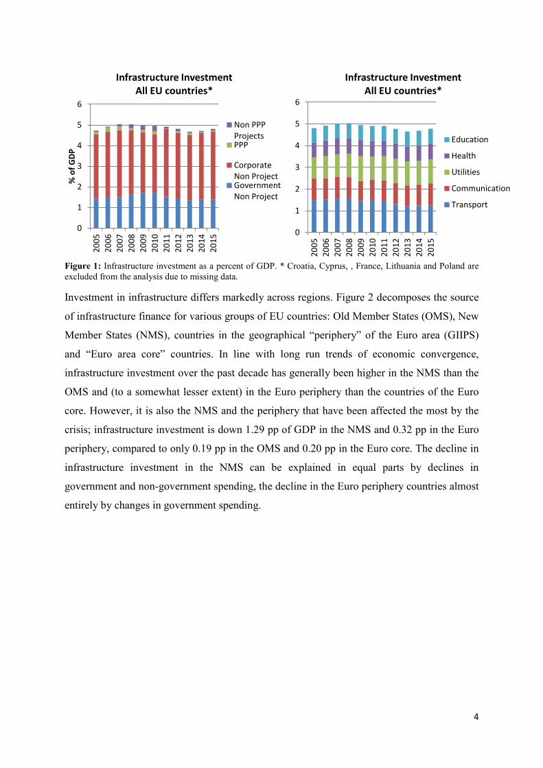
Figure 1 shows that infrastructure investment in the EU followed the business cycle closely
over the past decade, falling in the wake of the global financial crisis and again after the
sovereign debt crisis. The first phase of contraction was driven by private infrastructure
finance with public infrastructure investment remaining stable at first. However, with the
onset of the sovereign debt crisis in 2011 and 2012, this picture changed, with fiscal
consolidation acting pro-cyclically to deepen the decline in infrastructure investment. With
regard to sectors, the steady decline of investment in the transport sector is striking; while
transport accounted for 31% of total infrastructure investment in 2007 (corresponding to 1.6%
of GDP), it stood at only 26% in 2015 (1.3% of GDP).
6 As a starting point, we use national accounts statistics from Eurostat to construct estimates of total and government investment in infrastructure sectors. Private investment is then derived as a residual. We also provide a sectorial breakdown of these estimates using Eurostat data on gross fixed capital formation in individual infrastructure sectors, including education, health, transport, communication, and utilities. In a second step, we break down our (derived) infrastructure aggregates with the help of data from Projectware. This database allows us to identify investments made through Special Purpose Vehicles (SPVs, i.e. projects) and thus to identify corporate (non-project) infrastructure investment as the difference between total private and total project investments. Finally, we divide our project investment into Public-Private Partnership projects and non-PPP projects, using data described in Kappeler and Nemoz (2010). Since most PPP finance is entirely private, we approximate non-PPP private project finance simply as the difference between total private project investment and PPP investment.
4
Figure 1: Infrastructure investment as a percent of GDP. * Croatia, Cyprus, , France, Lithuania and Poland are excluded from the analysis due to missing data.
Investment in infrastructure differs markedly across regions. Figure 2 decomposes the source
of infrastructure finance for various groups of EU countries: Old Member States (OMS), New
Member States (NMS), countries in the geographical “periphery” of the Euro area (GIIPS)
and “Euro area core” countries. In line with long run trends of economic convergence,
infrastructure investment over the past decade has generally been higher in the NMS than the
OMS and (to a somewhat lesser extent) in the Euro periphery than the countries of the Euro
core. However, it is also the NMS and the periphery that have been affected the most by the
crisis; infrastructure investment is down 1.29 pp of GDP in the NMS and 0.32 pp in the Euro
periphery, compared to only 0.19 pp in the OMS and 0.20 pp in the Euro core. The decline in
infrastructure investment in the NMS can be explained in equal parts by declines in
government and non-government spending, the decline in the Euro periphery countries almost
entirely by changes in government spending.
0
1
2
3
4
5
620
0520
0620
0720
0820
0920
1020
1120
1220
1320
1420
15
% o
f GDP
Infrastructure Investment
All EU countries*
Non PPPProjectsPPP
CorporateNon ProjectGovernmentNon Project
0
1
2
3
4
5
6
2005
2006
2007
2008
2009
2010
2011
2012
2013
2014
2015
Infrastructure Investment All EU countries*
Education
Health
Utilities
Communication
Transport

5
Figure 2: Infrastructure investment as a percent of GDP, by source and region. *New Member States exclude Croatia, Cyprus, , Lithuania and Poland due to missing data. Old Member States and Core countries exclude France due to missing data.
Further light can be shed on these trends by examining them in real terms to exclude the effect
of changes in GDP. Figure 3 shows the evolution of real infrastructure investment for the
government and private sector and for key sectors: education, health, transport,
communication and utilities (including energy, water and waste). For ease of comparison, we
index real infrastructure investment to equal 100 in 2008. The figure indicates that real
government investment increased in 2008 to 2010 – acting counter-cyclically – while
corporate investment fell quite dramatically over this period. With the onset of the sovereign
debt crisis, this picture changed: the government sector cut back on its infrastructure
investment activity – while the corporate sector recovered somewhat (but only to cut back on
its investment in 2012 and 2013 again). Since 2013, both – real government investment and
corporate investment – have increased. However, real government infrastructure investment
01234567
% o
f GDP
Infrastructure Investment
New Member States*
Non PPP Projects PPPCorporate Non Project Government Non Project
01234567
Infrastructure Investment Old Member States*
Non PPP Projects PPPCorporate Non Project Government Non Project
0
1
2
3
4
5
6
% o
f GDP
Infrastructure Investment Core countries*
Non PPP Projects PPPCorporate Non Project Government Non Project
0
1
2
3
4
5
6
Infrastructure Investment GIIPS countries
Non PPP Projects PPPCorporate Non Project Government Non Project

6
in 2015 came still in below its 2008 level (-2.6%), whereas private investment is now higher
than in 2008 (+6.6%).
Figure 3: Real infrastructure investment, by source and sector
Figure 3 confirms that the sector hardest hit by the economic crises in real terms is transport
(down 10.8% from 2008). The other sectors showed more resilience. Indeed, investment in
education, health, communication and utility infrastructure even increased in real terms
(+10.1%, 1.4%, 7.9% and 11% respectively) compared to their 2008 level.
Figure 4: Real infrastructure investment, by region. * New Member States exclude Croatia, Cyprus, , Lithuania, Poland and Romania. Old Member States and Core countries exclude France due to missing data.
Figure 4 shows the evolution of real infrastructure investment by region. It shows that the
countries of the Euro Core were hit hard by the financial crisis of 2007-2008 but more
moderately by the sovereign debt crisis. For the GIIPS region, the opposite is true; they
exhibited some resilience after the financial crisis but the sovereign debt crisis lead to a sharp
80
85
90
95
100
105
110
Infrastructure Investment in real terms (2008 = 100)
Government Non Project Private Non Project
80
85
90
95
100
105
110
Infrastructure Investment in real terms (2008 = 100)
Transport CommunicationUtilities HealthEducation
70
80
90
100
110
2005 2006 2007 2008 2009 2010 2011 2012 2013 2014 2015
Infrastructure Investment in real terms (2008 = 100)
New Member States GIIPS countries Core countries

7
contraction in real infrastructure investment. Infrastructure investment was initially hardest hit
in the New Member States (-17.5% in 2012 relative to where they were in 2008). However,
their recovery started already in 2013, when the GIIPS region still experienced contractions.
Public-private partnerships (PPPs) represent a small component of the overall infrastructure
market but are seen as strategically important for infrastructure finance, particularly in the
light of the fiscal space constraints faced by public authorities. The total PPP market in
Europe has grown steadily over the past twenty years, reaching its historical peak in 2007 – at
around EUR 30bn.7 Since then, both the total number of deals and the aggregate value of
deals have declined considerably. In 2014, the aggregate market value achieved a total of
EUR 16bn, returning to positive growth in nominal terms for the second time after 2013 (and
a small bump in 2010).
Geographically, the PPP market remains highly concentrated. The UK is still the largest
European PPP market in 2013/2014 (EUR 6bn), although its share of the EU market has
declined to 35%, from 56% in 2007. The UK is followed by Italy (EUR 2.6bn), France (EUR
1.1bn) and the Netherlands (EUR 0.7bn). With EUR 9bn, the transport sector represents more
than half the total market value in 2013/2014.
PPP financing is dominated by debt. Figure 5 shows that the debt-to-equity ratio has come in
at around 5:1 over the past decade.8 Most of this debt is made up of loans (typically provided
through syndicates of lenders). While bond financing played an important role in providing
funding before the crisis – accounting for up to 19% of total financing and 22% of total debt
in 2007 – it disappeared almost completely in the period 2009-2012. In 2013 and 2014, bond
financing made a comeback contributing to almost 6%/13% of total PPP financing in the two
years. However, the use of project bonds is largely restricted to only four member States:
Germany, Netherlands, Spain and the United Kingdom.
7 For completeness, we also include PPPs in non-infrastructure related sectors. 8 Figure 5 uses the EIB ECON/EPEC database. Note that a breakdown by source of finance is only available for roughly 80% of all PPP projects in the database.

8
Figure 5: Financing structure of European PPP investments
The global financial crisis and the sovereign debt crisis have had a dramatic impact on the
cost of debt finance for PPPs. Figure 6 shows that spreads over Libor/Euribor declined in the
run-up to the financial crisis, from 110 basis points in 2000 to 80 basis points in 2007. The
financial crisis dramatically reversed this tendency as spreads tripled to more than 250 bps
between 2007 and 2010. After reaching a plateau in 2010/2011, there was another significant
increase – by almost 100 basis points – as the sovereign debt crisis hit in 2011/2012. 2013 and
2014 marked the first years since 2007 that prices weakened somewhat.
For comparison, Figure 6 also shows the weighted average of sovereign credit default swaps
as a broad measure of market condition.9 Pricing for PPP loans broadly moved in line with
CDS in the run up to the crisis – and during the initial crisis years – but there is a notable
divergence of the two measures in more recent years. While sovereign default swaps have
fallen markedly since 2011, PPP pricing have continued to rise initially and remained
relatively elevated since.
9 Figure 6 uses the EIB ECON/EPEC database. Data on pricing refer to the principle loan of each project as made available by Projectware and/or the Infrastructure Journal. As this information is available for a sub-sample only, the results should be taken as indicative rather than definitive. For CDS, we use 5 year sovereign CDS from Bloomberg.
0%
20%
40%
60%
80%
100%
Financial Structure of PPPs
Loan Bond Equity

9
Figure 6: Pricing of PPPs
The trends clearly show the impact of financing constraints on the infrastructure sector. In the
wake of the crisis, many Member States and sub-sovereigns find themselves with less fiscal
space for direct funding through budgets or the provision of risk-taking equity in PPP
schemes. At the same time, several major banks have retreated from the infrastructure
investment field or have become more selective, possibly reflecting enhanced capital
constraints faced by the European banking sector. While European banks are now generally
well capitalised in terms of CET1 capital ratios, the space they have to expand their balance
sheets or to shift from low risk sovereign holdings to higher risk investments including project
lending is limited.
The situation for infrastructure investors has been compounded by the decline of monoline
insurers. This has reduced the availability of credit insurance which played a crucial role in
enhancing credit quality of infrastructure investment and thereby pulled in investors that
sought limited exposure to risks. Whilst there has been some market recovery and liquidity
has returned to some sectors of some markets, many projects, perceived as carrying higher
risk (e.g. risk associated with greenfield projects, the predictability of demand, the very long-
term development period, or the cross-border element of the project), are still unable to secure
adequate funding. Institutional investors, including insurance corporations and pension funds,
are a potentially important source of finance for infrastructure projects that offer long-term
assets to match their long-term liability structure. However, the involvement of institutional
investors remains weak.
050
100150200250300350400
Average Pricing PPPs
average pricing, PPPs CDS (weighted average)

10
The lack in many countries of a strong pipeline of projects structured in a suitable way to
attract private investors, as well as the uncertainty related to the macroeconomic environment
and regulatory stability have also been identified as an important constraints on infrastructure
finance. To address these issues effectively, the Investment Plan for Europe intends to
combine regulatory reforms in EU countries, better support and advisory for project
preparation, and the European Fund for Strategic Investment (EFSI) implemented by the EIB.
3. Investigating the importance of transport infrastructure: linking local business with global growth opportunities
Transport is the largest infrastructure sectors (in terms of investment) and it has been affected
particularly severely by the economic crisis. In the following sections, we take transport as an
example and examine one important way in which investment in infrastructure can contribute
to economic recovery.
Using data on 245 European regions, we show that transport infrastructure plays a role in
explaining why firms in some regions are better placed in capitalising on global growth
opportunities than firms in other regions. We also find that the positive effects of a well-
developed transport stock are particularly pronounced in regions where there is ‘economic
slack’. This suggests that a higher transport network can act as a catalyser for economic
recovery in times of stress. In other words, a poor infrastructure stock may hamper economic
recovery by cutting the link between local businesses and their global growth opportunities.
Our study builds on a long history of literature going back to the founders of trade theory and
microeconomics. Heckscher (1916), for example, qualified many of his early arguments about
the resource basis for trade with caveats about initial physical conditions that might facilitate
or hinder trade relations. A variety of authors, including Obstfeld and Taylor (1997), have
implemented Heckscher’s notion in an empirical application. Samuelson (1952) made an
early contribution to economic and trade analysis from a spatial perspective – which was also
followed by many contributions from regional analysis and location theory (e.g. Bergstrand
1990) and directly inspires the current study.
While our study builds on this literature, it also expands on it in several ways. Most
importantly: (i) the paper is the first (to the best of our knowledge) to examine the importance
of regional transport infrastructure when it comes to linking local business to global growth

11
opportunities in the context of European regions; and (ii) we use a direct measure of global
growth opportunities (instead of an indirect measure, such as trade flows).
4. Conceptual Framework
To measure global growth opportunities, we build on Bekaert et al. (2007) – who recently
proposed a measure of global growth opportunities based on global industry price to earnings
(PE) ratios weighted by the local industry mix within a particular country. They argue that
their measure is a good predictor of economic growth. More specifically, they find that
countries with a high concentration of high PE industries (using global industry PE ratios)
grow faster on average. Using data on 245 European regions over the period 2002 to 2013, we
show in Table 1 that such global growth opportunities also predict economic activity at the
regional level.
Table 1. Global growth opportunities are associated with regional economic activity. Dependent variable: regional GDP growth and change in the regional unemployment rate
GDP growth Unemployment Global Growth Opportunity 0.011*** -0.146*
(0.003) (0.079)
Sample size 2,444 2,468 R-squared 0.033 0.003 Number of regions 245 245
Note: All regressions control for region fixed effects. Unbalanced panel. Time period: 2002-2013. Robust standard errors in parentheses. *** p<0.01, ** p<0.05, * p<0.1.
However, not all regions benefit from global growth opportunities in the same way. Figure 7
illustrates the difference between the growth rates predicted by our measure of global growth
opportunities and the actual growth rates of different European regions over the time period
2002-2013. It suggests that some regions did a lot better in terms of actual growth rates than
what one might have expected given their global growth prospects; while others did a lot
poorer – which raises the question: what determines the extent to which a region manages to
benefit from positive global growth opportunities?

12
Figure 7: Average difference in predicted and actual growth rates. Dependent variable: GDP growth. Explanatory variable: Global growth opportunities and region fixed effects
This paper also takes inspiration from classical trade theory which states that price differences
create incentives for international and inter-regional exchange of goods.10 According to this
view, high distribution margins (due, for instance, to poor infrastructure) serve to undermine
these price differences and, thus, the basis for trade.
To see this, consider two prices PH and PF for comparable goods from two different sources:
home and foreign (although they could simply be from different regions or even cities in the
same country). Given that a trade margin (M) is generally symmetric, the ratio of these two
prices is given by the following expression, evaluated as M rises without limit:
𝑃𝐻+M𝑃𝐹+M
1 (1)
Evidently, if there is a poor transport network in a region, then the margin will be higher (for
instance, because of higher accessibility costs) and it will be more costly for a local firm to
serve markets beyond its immediate surrounding. Similarly, and because the trade margin is
symmetric, it will be more costly for a non-local firm, in such a situation, to serve the local
market.
This effect is accentuated by the fact that, at the same time, higher margins worsen terms of
trade. Consider the local producer price of exports PE=PWE-M, where PWE denotes the
10 See, e.g., Roland-Holst (2009) for a review.

13
international price of an export good and M the margin on an exporter’s net revenue (producer
price). Symmetrically, the local purchaser price of imports takes the form PM=PWM+M where
PWM is the corresponding international price of imported goods and the margin M must be
added to purchaser prices.
M↑ 𝑃𝑊𝑊−M𝑃𝐷
↓ and 𝑃𝑊𝑊+M𝑃𝐷
↑ (2)
This suggests that higher margins (due to poorer regional infrastructure and higher
accessibility costs) induce an increase in terms of trade PE/PM – and so reduce the incentive to
trade.
There are several hypotheses that can be derived from this basic idea:
1. Hypothesis 1: Everything else equal, an exogenous shock to a region’s global growth
opportunities will have a different impact on economic activity depending on a
region’s transport infrastructure. A positive shock will have a stronger positive effect
on output and unemployment in regions with good transport infrastructure. A negative
shock will not be amplified by a higher transport infrastructure (and may even be
mediated by a higher transport stock).
If a positive demand shock occurs, our conceptual framework suggests that firms in regions
with a higher stock of regional infrastructure will be better placed to benefit from this shock
in terms of output and unemployment than the same firms in regions with low regional
infrastructure. They will have better access to local and global markets (both in terms of
attracting resources and distributing output) to exploit such shocks.
A negative shock in terms of global growth opportunities, on the other hand, will not translate
into a stronger negative effect in regions with good transport infrastructure. While it is true
that being more closely integrated into global markets means that regions with a higher
transport stock are likely to be affected more immediately, it is also the case that, insofar as a
negative shock means that supply will be priced out of global markets, the first ones to suffer
from this will be the regions where marginal costs are highest. As a result, the negative effect
on export (and import) prices should make regions with low transport infrastructure at least as
vulnerable to a negative shock as(and possibly even more vulnerable than) regions with a high
transport stock.11
11 Given the focus on European regions, which tend to be globally relatively well integrated, we expect that the ‘price effect’ (of being priced out first) outweighs the ‘quantity effect’ (of being less integrated to start with).
14
2. Hypothesis 2: Everything else equal, we expect that ‘economic slack’ accentuates the
role played by regional transport infrastructure in case of a positive exogenous shock
– making infrastructure an important ingredient for a fast economic recovery.
Assuming that prices respond less to positive growth opportunities in regions in which there is
‘economic slack’ (as defined in detail later), we expect that better regional infrastructure
translates into higher economic benefits for local firms (given a positive shock to their global
growth opportunities) if there is economic slack than when there is not. The intuition would
be as follows: any expansion of production at or above full capacity is likely to involve
significant upward pressure on prices which undermines (at least in part) the advantage of
lower margins (due to a better transport network) and, hence, international competitiveness.
A further issue is whether a shock to global growth opportunities can be expected to have
spill-over effects in neighbouring regions. While beyond the scope of this paper, we also
examine in Revoltella et al. (Forthcoming) the hypothesis that the level of transport stock in
neighbouring regions will enhance the likelihood of spill-overs from a positive shock and
have no effect on any spill-overs from a negative shock.
5. Empirical framework
This section provides an empirical strategy on how to test hypotheses 1 and 2. The general
idea is to explore whether and to what extent regions’ with a higher stock of transport
infrastructure are better placed to benefit from positive shocks to global growth opportunities
while not being more affected by (or possibly even being shielded from) adverse shocks. The
basic empirical model takes the following form:
∆𝐺𝐺𝐺𝑖,𝑡 = 𝛼𝑖 + 𝛽1𝐺𝐺𝐺𝑖,𝑡−1 + 𝛽2𝑇𝑇𝑖 + 𝛽3�𝐺𝐺𝐺𝑖,𝑡−1𝑥𝑇𝑇𝑖� + 𝜀𝑖,𝑡 (3)
∆𝑢𝑢𝑢𝑢𝑢𝑢𝑢𝑢𝑖,𝑡 = 𝛼𝑖 + 𝛽1𝐺𝐺𝐺𝑖,𝑡−1 + 𝛽2𝑇𝑇𝑖 + 𝛽3�𝐺𝐺𝐺𝑖,𝑡−1𝑥𝑇𝑇𝑖� + 𝜀𝑖,𝑡 (4)
where i = 1, ..., R denotes the regions, t = 1, …, T the time periods, 𝛼𝑖 captures regional fixed
effects, 𝐺𝐺𝐺𝑖,𝑡−1 is the proxy for global growth opportunities (in logarithm), 𝑇𝑇𝑖 is an
indicator variable denoting a high stock of transport infrastructure and �𝐺𝐺𝐺𝑖,𝑡−1𝑥𝑇𝑇𝑖� is the
interaction term between these two last variables.12
12 Global growth opportunities (GGO) enter our specification with a one period lag (just as in Bekaert et al., 2007) because changes in production tend to take time to be put in place (in particular if they are associated with capacity extension).

15
To distinguish between positive shocks and negative shocks (hypothesis 1), we compare the
pre-crisis (2003-2007) and the (post-)crisis periods (2008-2012).13 To determine whether the
role of transport infrastructure varies with the level of ‘economic slack’ in a region’s economy
(hypothesis 2), we divide the sample based on an indicator variable capturing the degree of
employment slack in a region.
Given our two first hypotheses and the model specification, Table 2 summarises the expected
signs on the interaction term in the basic model. All signs are stated for GDP growth as the
dependent variable but the opposite signs apply for regional unemployment as the dependent
variable. Our theoretical framework suggests that the interaction term between the measure of
global growth opportunities and transport infrastructure �𝐺𝐺𝐺𝑖,𝑡−1𝑥𝑇𝑇𝑖� should be positive in
case of a positive shock to a region’s global growth opportunities and negative (or
insignificant) in case of a negative shock. In the first case, a better transport network should
accentuate the positive shock; in the second case, it should mediate the negative shock (or at
least not amplify it).
Table 2. Expected sign on the interaction term between global growth opportunities (GGO) and transport infrastructure. Dependent variable: regional GDP growth
Type of shock: Positive
Negative Transport stock: High
Low
High
Low
�𝐺𝐺𝐺𝑖 ,𝑡−1𝑥𝑇𝑇𝑖� ++ -/0 �𝐺𝐺𝐺𝑖 ,𝑡−1� + ++
Note: ++: large increase; +: limited increase; –: limited decrease; ––: large decrease.
The expected sign on the coefficient of global growth opportunities (GGO) is the same
whether it captures a positive shock or a negative one – as we assume that a positive
(negative) shock will lead to higher (lower) growth even in regions with low regional
infrastructure.
Table 3 summarises the expected signs on the coefficients in the version of the model that
accounts for slack. In case of a positive economic shock, the coefficient on the interaction
term between global growth opportunities (GGO) and the transport stock should be positive,
both in the case of economic slack and in the absence of economic slack. This is because we
expect a positive shock to translate into higher growth in both cases. However, the magnitude
13 Instead of focusing on the pre-crisis and (post-)periods, we also estimated the model using a panel of regions experiencing positive shocks to their global growth opportunities and a panel of regions experiencing negative shocks to their global growth opportunities (GGO), respectively. That is, as a robustness check, we focus on regions with strokes of positive (or negative) global growth opportunities (GGO) over several consecutive years and find that the results are in line with those reported here.

16
of the coefficients is expected to differ. We expect a larger coefficient when there is slack
(than when there is not) – as, at or above full capacity, higher prices are likely to diminish the
positive effect of a better transport stock.
Table 3. Expected sign on the interaction term between global growth opportunities (GGO) and the transport stock when there is economic slack. Dependent variable: regional GDP growth
Positive Shock Economic slack: Yes
No
Transport stock: High
Low
High
Low �𝐺𝐺𝐺𝑖 ,𝑡−1𝑥𝑇𝑇𝑖� ++ + �𝐺𝐺𝐺𝑖 ,𝑡−1� + +/0
Negative Shock Economic slack: Yes
No
Transport stock: High
Low
High
Low �𝐺𝐺𝐺𝑖 ,𝑡−1𝑥𝑇𝑇𝑖� -/0 -/0 �𝐺𝐺𝐺𝑖 ,𝑡−1� ++ ++
Note: ++: large increase; +: limited increase; –: limited decrease; ––: large decrease.
In the case of a negative shock, we expect an insignificant (or negative) coefficient because
we expect a higher transport stock to not amplify (and possibly mediate) the negative
consequences of a deterioration of global growth prospects. Due to price stickiness, we do not
expect any difference between situations with high or low economic slack.14
The coefficient on global growth opportunities (GGO) is likely to be positive if there is
economic slack and insignificant otherwise. In case of a negative shock, we expect a positive
coefficient irrespective of whether there is economic slack: a negative development of global
growth prospects should affect regions (with a low transport stock) in the same way whether
or not they suffer from economic slack.
6. Data and results
This section describes the variables used in the empirical analysis and reports regression
results based on the empirical framework discussed in the previous section. We use annual
data at regional level. We rely on an unbalanced panel dataset covering 245 regions in 19 EU
14 Given a certain stickiness of prices when it comes to negative shocks, we expect to find no difference in the effect of a negative change in global growth opportunities for firms in regions in which there is ‘economic slack’ and firms in regions where there is not. See Blinder (1998) for an overview of the related literature.

17
countries over the time period 2002 to 2013.15 Table A.1 in Appendix 1 gives more details on
the source of the data and Table A.2 reports descriptive statistics.
Dependent variables: To determine whether and to what extent the level of transport stock in
a region can affect how an exogenous shock to a region’s global growth opportunities
translates into regional economic activity, we use regional real GDP growth and the change in
the regional unemployment rate as dependent variables.
Global growth opportunities: To proxy for global growth opportunities in each region in the
sample, we follow Bekaert et al. (2007) and use global price-to-earnings (PE) ratio weighted
by the regional industry mix. We use global PE ratios of 25 industries in the manufacturing
sector.16 We weight the importance of each industry using the salary share of each industry
out of total salaries in a region. Intuitively, our measure, thus, takes each region as a
composition of sectors with different growth opportunities (captured by investors’
expectations about their future growth potential). Because the PE ratios are global, the proxy
measures exogenous growth opportunities rather than region-specific growth opportunities.
High stock of regional transport infrastructure: To capture the level of regional transport
infrastructure, we aggregate the average number of kilometres of roads, motorways and rail
lines between 2002 and 2013. We divide this measure of distance by the average of the
regional population between 2002 and 2013. We then create an indicator variable equal to 1 if
a region’s transport stock density is in the upper tercile of the overall transport stock density
distribution and 0 otherwise.17 This creates a measure of transport stock density in a region
weighted by its population. The measure is by construction time-invariant over the period that
we consider. The transport stock tends to vary rather slowly and our transport stock variable is
discrete.
Positive vs negative shocks: To capture the different effects of a positive and negative
exogenous shocks to regions’ global growth opportunities, we use the pre-crisis period (2003-
15 We follow the EU classification of regions and use NUTS at level 2. There are 273 regions at NUTS level 2 in the EU28. We had to exclude 9 EU member states because of missing data at the regional level on some of the variables used in the analysis. 16 We focus on the manufacturing sector as Bekaert et al. (2007) argue that their measure is a better predictor of economic activity for open economies and industries. 17 All the results reported in this paper are robust to an alternative definition of the indicator variable for the transport stock where we use the upper quartile of the transport stock density distribution (instead of the upper tercile).

18
2007) and the (post-)crisis period (2008-2013) to distinguish between an environment with
(largely) positive and (largely) negative global growth opportunities.18
Economic slack: To proxy for economic slack, we use the distance to ‘full employment’ for
each region. Specifically, we calculate the difference between the regional unemployment rate
in each year and its average unemployment rate between 2002 and 2013.19 Similarly to the
transport stock density variable, we create an indicator variable equal to 1 if a region’s
unemployment gap is positive and in the upper tercile of the sample-wide unemployment gap
distribution and 0 otherwise.20
The first column in Table 4 finds that the interaction term between the proxy for global
growth opportunities and the transport stock is positive and statistically significant for GDP
growth; and negative and statistically significant for unemployment. This is broadly in line
with our hypothesis.21
Table 4. The interaction term between the proxy for global growth opportunities and the transport stock is associated with regional economic growth and unemployment. Dependent variable: regional GDP growth and change in the regional unemployment rate
GDP growth Unemployment Global Growth Opportunities 0.007** -0.090
(0.003) (0.078)
GGO x Transport stock 0.041*** -0.563*** (0.006) (0.158) Sample size 2,444 2,468 R-squared 0.075 0.007 Number of regions 245 245
Note: All regressions control for region fixed effects. Unbalanced panel. Time period: 2002-2013. Robust standard errors in parentheses. *** p<0.01, ** p<0.05, * p<0.1.
When focus on instances with mostly positive shocks to global growth opportunities, we find
that that the interaction term is also positive and statistically significant when the dependent
18 As discussed above, as robustness check, we also identify all those instances where a region had a PE ratio in the top (and bottom) tercile of PE ratios in at least 4 out of 6 years and assembles these instances to create a panel consisting only of regions affected by positive (negative) shocks to their global growth opportunities. 19 A comparison of the average unemployment rate with European Commission estimates of the natural rate of unemploy-ment at the national level confirms that the average unemployment rate is a good proxy for the natural rate of unemployment (and hence full employment). 20 In view of better reflecting national differences in the labour market structure, we also use an indicator variable equal to 1 if a region’s unemployment gap is positive and in the upper tercile of the country’s unemployment gap over the period 2002 and 2013. The results are not affected by this alternative definition of employment slack. The results are also robust to an alternative definition of employment slack where we use the employment rate instead of the unemployment rate. In this case, the indicator variable for slack is equal to 1 if a region’s employment gap is negative and in the lower tercile of the European or country-specific employment gap distribution. 21 When we use country fixed effects (instead of region fixed effects) or add year fixed effects to the model, we also find that the estimated coefficient on the interaction term is always positive and statistically significant.

19
variable is output growth (see Table 5).22 For the sake of brevity, we focus on GDP growth
but the results are similar when use the change in unemployment as the dependent variable
(i.e. the estimated coefficients have the opposite sign). This suggests that regions with a high
stock of transport infrastructure are better placed to benefit from positive global growth
opportunities.
Given that the coefficients on the global growth opportunities are insignificant in our ‘positive
growth’ scenario, the estimates also show that, on average, only regions with a high stock of
transport infrastructure are able to significantly benefit from positive global growth
opportunities. For regions with a low transport infrastructure, a positive shock to global
growth opportunities does not seem to translate into any material improvement with respect to
growth.
If we focus on a negative shock environment, we find that negative changes to global growth
opportunities translate into negative outcomes in GDP growth. This is the case both for
regions with a high level of transport shock and regions with a low level of transport stock –
which means that while a high transport stock does not amplify the negative consequences of
a deterioration global growth outlook it does not mediate them either.
Table 5. The interaction term between the proxy for global growth opportunities and the transport stock is associated with regional economic growth only before the crisis. Dependent variable: regional GDP growth
Pre-crisis
(2003-2007) (Post-)crisis (2008-2012)
Global Growth Opportunities 0.001 0.046***
(0.002) (0.003)
GGO x Transport stock 0.017** 0.002 (0.009) (0.007) Sample size 1,050 1,050 R-squared 0.006 0.325 Number of regions 210 210
Note: All regressions control for region fixed effects. Balanced panel. Time period: 2003-2012. Robust standard errors in parentheses. *** p<0.01, ** p<0.05, * p<0.1.
In Table 6, we test whether employment slack affects the role played by the region’s transport
stock in case of an exogenous shock. We find that the simple interaction term (𝐺𝐺𝐺𝑖,𝑡−1𝑥𝑇𝑇𝑖)
has the same positive sign, both in case of slack and in the absence of slack. However, and in
line with our second hypothesis, we find that the transport network has a larger impact on
22 The estimates in Table 5 use a balanced panel over the period 2003-2012 so that the same regions are included in the pre-crisis period and (post)crisis period. The results using an unbalanced panel over the period 2002-2013 are qualitatively simi-lar.

20
economic activity in regions with employment slack (making it a possible source for faster
economic recovery) – as the difference between the two coefficients is statistically significant.
Table 6. The size of the interaction term between the proxy for global growth opportunities and the transport stock is larger in regions with economic slack. Dependent variable: regional GDP growth
Slack No slack
Global Growth Opportunities 0.010** 0.009**
(0.004) (0.004)
GGO x Transport stock 0.062*** 0.030*** (0.011) (0.007) Sample size 880 1,562 R-squared 0.195 0.063 Number of regions 241 235
Note: All regressions control for region fixed effects. Balanced panel. Time period: 2002-2012. Robust standard errors in parentheses. *** p<0.01, ** p<0.05, * p<0.1.
Figure 8 illustrates this result by means of simple plot of the regression outcome. It shows that
the effect of an exogenous shock to global growth opportunities is larger in regions with a
high transport stock, regardless of the degree of economic slack inherent in the regions.
However, the effect is even more pronounced in regions suffering from economic slack –
suggesting that having a high regional transport stock may be an important ingredient for
economic recovery.
Figure 8: Average marginal effects of the PE ratio on regional GDP growth and unemployment in regions where there is employment slack and in the absence of employment slack
A detailed analysis (distinguishing between positive and negative shock scenarios and taking
slack into account) also shows that the amplifying effect of a higher transport stock holds
0
0.02
0.04
0.06
0.08
no slack slack
Effe
ct o
n GD
P gr
owth
low transport stock high transport stock

21
when there are positive shocks to global growth opportunities (only). The case of negative
shocks is more problematic to examine as periods with primarily negative shocks tend to
come with high slack – and a comparison with no slack is, therefore, difficult.
7. Conclusion
This paper finds evidence for the hypothesis that the regional transport stock matters to link
local businesses with global growth opportunities. More specifically, we show that an
increase in exogenous global growth opportunities translates into stronger economic growth in
regions with a better transport network. This effect is particularly pronounced in periods of
economic slack – when, arguably, there are sufficient resources available to expand capacity.
A deterioration in global growth opportunities, however, does not translate into a worse
growth performance for regions with a higher transport stock. This suggests that the effect of
a good transport network in absorbing global growth shocks is not symmetric. A higher
transport stock benefits a region in times of positive shocks, but does not make it worse off in
times of a negative shock.
Combined with our findings from the first part of the paper – that infrastructure investment in
Europe has been on a downward trend for several years, this raises concern whether this may
have already affected (or may sometimes soon constraint) the capacity of local firms in the
EU to benefit from global growth opportunities. It also raises an additional question: what is
holding back investment in transport infrastructure in Europe?
Limited fiscal space is an important constraining factor. While it is true that the importance of
private finance in the transport sector has grown over the last two decades, mainly in the form
of Public Private Partnerships (PPP), it would need to increase much further to compensate
for the lack of public funds. The EIB, in collaboration with the European Commission, has
developed over the years innovative financial instruments for more capital market as well as
more bank participation in the funding of infrastructure projects.
In addition, the European Fund for Strategic Investment (EFSI), established as the main
element of the Investment Plan for Europe, aims to mobilise some EUR 315 billion of
investment over three years (a large part of which will come from private sources), helping to
address key market gaps and structural weaknesses to build a more competitive EU economy.

22
The EFSI is funded by EUR 16 billion in guarantees from the EU budget and EUR 5 billion
from the EIB’s own funds.
But there are many other bottlenecks for additional investment apart from funding. An
inappropriate regulatory environment is one of the most important constraints to the
development of key transport infrastructure projects – in particular with regard to permitting
and procurement procedures. Regulatory barriers induce very long lead times and delays,
sometimes amounting to decades, with a very high opportunity cost for society. This is even
more acute for cross-border projects where the differences in national systems and law
accentuate the obstacles faced. A lack of harmonised standards at the European level can also
hinder project implementation, while uncertainties related to tariff regimes can be a
significant deterrent to private investors.
Last but not least, it is important to bear in mind that adequate funding and a proper
regulatory framework can do only so much when it comes to promoting the development of
additional transport infrastructure. An economically sound preparation of projects matters as
well. There are already several initiatives that try to address this issue, and clearly more could
be done. For instance, the JASPERS initiative has been instrumental in providing advice to
EU member states with regard to project preparation. The European PPP Expertise Centre
(EPEC) has also played a key role in developing the capacity of public sector entities to
implement PPP projects and programmes. These and other technical advisory services will be
brought together to form a European Investment Advisory Hub to create a one-stop-shop for
project promoters to receive support in the context of the Investment Plan for Europe.

23
References
Bekaert, G., Harvey, C.R., Lundblad, C., and Siegel, S. (2007). Global growth opportunities and market integration. Journal of Finance, 62(3), 1081-1137.
Bergstrand, J.H. (1990). The Heckscher-Ohlin-Samuelson model, the Linder hypothesis and the determinants of bilateral intra-industry trade. Economic Journal, 100(403), 1216-1229.
Berndt et al. (2015). Restoring EU competitiveness. European Investment Bank, Luxembourg.
Blinder, A., Canetti, E.R.D., Lebow, D.E., and Rudd, J.B. (1998). Asking about prices: A new approach to understanding price stickiness. Russell Stage Foundation, New York.
Hätönen, J. (2011). The economic impact of fixed and mobile high-speed networks. EIB Papers, 16(2), 30-59.
Heckscher, E.F. (1916). Vaxelkursens grundval vid pappersmyntfont. Ekonomisk Tidskrift, 18, 309–312.
Kappeler, A. and Nemoz, M. (2010). Public-Private Partnerships in Europe – before and during the recent financial crisis. EFR 2010/4, European Investment Bank.
Obstfeld, M., and Taylor, A.M. (1997). Nonlinear aspects of goods-market arbitrage and adjustment: Heckscher's commodity points revisited. Journal of the Japanese and International Economies, 11(4), 441-479.
Revoltella, D., Brutscher, P.B., Tsiotras, A. and Weiss, C.T. (Forthcoming). Linking local business with global growth opportunities: The role of infrastructure. Oxford Review of Economic Policy
Roland-Holst, D. (2009). Infrastructure as a catalyst for regional integration, growth, and economic convergence: Empirical evidence from Asia. In Fan Z. (ed.), From Growth to Convergence: Asia’s Next Two Decades, Palgrave Macmillan, New York.
Samuelson, P.A. (1952). The transfer problem and transport costs: The terms of trade when impediments are absent. Economic Journal, 62(246), 278-304.
Wagenvoort, R., de Nicola, C. and Kappeler, A. (2010). Infrastructure finance in Europe: Composition, evolution and crisis impact. EIB Papers, 15(1), 16-39.
WEF (2011). Advancing cloud computing: What to do now? Priorities for industry and governments. Report by the World Economic Forum in partnership with Accenture, Geneva.
24
Appendix 1
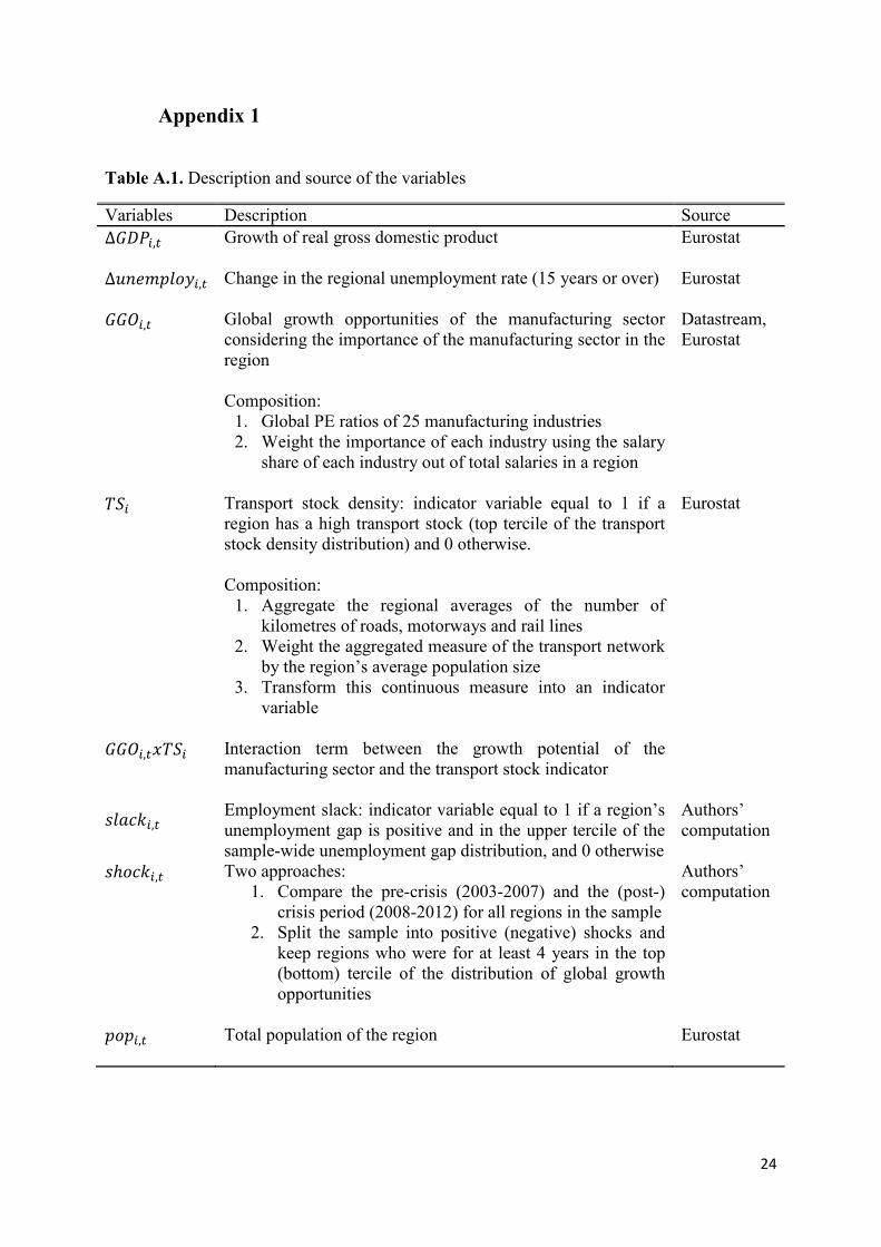
Table A.1. Description and source of the variables
Variables Description Source ∆𝐺𝐺𝐺𝑖,𝑡 Growth of real gross domestic product
Eurostat
∆𝑢𝑢𝑢𝑢𝑢𝑢𝑢𝑢𝑖,𝑡 Change in the regional unemployment rate (15 years or over)
Eurostat
𝐺𝐺𝐺𝑖,𝑡 Global growth opportunities of the manufacturing sector considering the importance of the manufacturing sector in the region Composition:
1. Global PE ratios of 25 manufacturing industries 2. Weight the importance of each industry using the salary
share of each industry out of total salaries in a region
Datastream, Eurostat
𝑇𝑇𝑖 Transport stock density: indicator variable equal to 1 if a region has a high transport stock (top tercile of the transport stock density distribution) and 0 otherwise. Composition:
1. Aggregate the regional averages of the number of kilometres of roads, motorways and rail lines
2. Weight the aggregated measure of the transport network by the region’s average population size
3. Transform this continuous measure into an indicator variable
Eurostat
𝐺𝐺𝐺𝑖,𝑡𝑥𝑇𝑇𝑖 Interaction term between the growth potential of the manufacturing sector and the transport stock indicator
𝑠𝑢𝑠𝑠𝑠𝑖,𝑡
Employment slack: indicator variable equal to 1 if a region’s unemployment gap is positive and in the upper tercile of the sample-wide unemployment gap distribution, and 0 otherwise
Authors’ computation
𝑠ℎ𝑢𝑠𝑠𝑖,𝑡
Two approaches: 1. Compare the pre-crisis (2003-2007) and the (post-)
crisis period (2008-2012) for all regions in the sample 2. Split the sample into positive (negative) shocks and
keep regions who were for at least 4 years in the top (bottom) tercile of the distribution of global growth opportunities
Authors’ computation
𝑢𝑢𝑢𝑖,𝑡 Total population of the region
Eurostat

25
Table A.2. Descriptive statistics
N Mean SD Min Median Max GDP growth 2,444 0.01 0.04 -0.15 0.01 0.19 Unemployment rate 2,468 8.59 4.69 1.90 7.50 36.20 Price to earnings (PE) ratio 2,400 18.47 3.60 9.87 19.06 33.37 PE ratio - manufacturing 2,374 19.36 5.17 7.94 19.37 45.23 Transport stock (in km) 2,468 16,972 17,413 31 11,703 94,336 Population (in thousand) 2,468 1,952 1,521 124 1,586 11,604


Economics DepartmentU [email protected]/economics
Information Desk3 +352 4379-220005 +352 4379-62000U [email protected]
European Investment Bank98-100, boulevard Konrad AdenauerL-2950 Luxembourg3 +352 4379-15 +352 437704www.eib.org
© EIB 07/2016 EN © EIB GraphicTeam


