
Information Transmission Using the Nonlinear FourierTransform
by
Mansoor Isvand Yousefi
A thesis submitted in conformity with the requirementsfor the degree of Doctor of Philosophy
Graduate Department of Electrical and Computer EngineringUniversity of Toronto
c© Copyright 2013 by Mansoor Isvand Yousefi

Abstract
Information Transmission Using the Nonlinear Fourier Transform
Mansoor Isvand Yousefi
Doctor of Philosophy
Graduate Department of Electrical and Computer Enginering
University of Toronto
2013
The central objective of this thesis is to suggest and develop one simple, unified method
for communication over optical fiber networks, valid for all values of dispersion and
nonlinearity parameters, and for a single-user channel or a multiple-user network. The
method is based on the nonlinear Fourier transform (NFT), a powerful tool in soliton
theory and exactly solvable models for solving integrable partial differential equations
governing wave propagation in certain nonlinear media. The NFT decorrelates signal
degrees of freedom in such models, in much the same way that the Fourier transform
does for linear systems. In this thesis, this observation is exploited for data transmission
over integrable channels such as optical fibers, where pulse propagation is governed by the
nonlinear Schrodinger (NLS) equation. In this transmission scheme, which can be viewed
as a nonlinear analogue of orthogonal frequency-division multiplexing commonly used in
linear channels, information is encoded in the nonlinear spectrum of the signal. Just as
the (ordinary) Fourier transform converts a linear convolutional channel into a number of
parallel scalar channels, the nonlinear Fourier transform converts a nonlinear dispersive
channel described by a Lax convolution into a number of parallel scalar channels. Since,
in the spectral coordinates the NLS equation is multiplicative, users of a network can
operate in independent nonlinear frequency bands with no deterministic inter-channel
interference. Unlike most other fiber-optic transmission schemes, this technique deals
with both dispersion and nonlinearity directly and unconditionally without the need for
dispersion or nonlinearity compensation methods. This thesis lays the foundations of
such a nonlinear frequency-division multiplexing system.
ii

Acknowledgements
First I wish to thank my advisor, Professor Frank R. Kschischang, for his excellent
academic supervision during the course of my doctoral work. Frank is a superb teacher
and a brilliant researcher from whom I learned enormously. He donates countless hours
training and educating his students and closely supervising them. His clarity of thought,
profound intuition and fundamental attitude toward problems have been a source of
inspiration. I am deeply indebted to him for many helpful and stimulating meetings that
we have had in the past years. The pleasant ambiance that he has created in his research
group and his generous financial support have made my time at the University of Toronto
a joyful experience.
I also wish to express my gratitude to the members of my Ph.D. committee, namely,
Professors Ashish Khisti, Raymond Kwong, Lacra Pavel, and Wei Yu. I wish to extend my
deep appreciation to Professor Andrew C. Singer, from University of Illinois at Urbana-
Champaign, both for agreeing to serve as my external examiner, and particularly for his
careful reading of the dissertation and his many constructive comments.
I am grateful to the University of Toronto for funding my Ph.D. program. This thesis
would not have been possible without financial support from the Government of Canada
and private donors of student scholarships. I acknowledge the Qureshi family for their
continued commitment to the student scholarships for the Communications Group.
Finally, I thank my friends and colleagues for the fun times, which will leave many
fond memories.
iii

Contents
1 Introduction 1
1.1 Related Work . . . . . . . . . . . . . . . . . . . . . . . . . . . . . . . . . 2
1.2 Contributions . . . . . . . . . . . . . . . . . . . . . . . . . . . . . . . . . 3
1.3 Thesis Outline . . . . . . . . . . . . . . . . . . . . . . . . . . . . . . . . . 4
1.4 Notation . . . . . . . . . . . . . . . . . . . . . . . . . . . . . . . . . . . . 5
2 Preliminaries 6
2.1 Origin of Information Theory . . . . . . . . . . . . . . . . . . . . . . . . 6
2.1.1 Statistical Regularity and the Concentration of Measure . . . . . 8
2.1.2 Information Theory and Noise . . . . . . . . . . . . . . . . . . . . 11
2.1.3 Communication Theory and Interference . . . . . . . . . . . . . . 21
2.2 Evolution Equations . . . . . . . . . . . . . . . . . . . . . . . . . . . . . 23
2.2.1 Dispersion Relations . . . . . . . . . . . . . . . . . . . . . . . . . 24
2.2.2 Classification of Evolution Equations . . . . . . . . . . . . . . . . 27
2.3 Lightwave Communications . . . . . . . . . . . . . . . . . . . . . . . . . 32
2.3.1 Components of a Fiber-optic System . . . . . . . . . . . . . . . . 33
2.3.2 Simplified Derivation of the NLS Equation . . . . . . . . . . . . . 38
2.4 Summary . . . . . . . . . . . . . . . . . . . . . . . . . . . . . . . . . . . 41
3 Origin of Capacity Limitations in Fiber-optic Networks 42
3.1 Capacity of WDM Optical Fiber Networks . . . . . . . . . . . . . . . . . 43
3.2 The Importance of the Inter-channel Interference . . . . . . . . . . . . . 49
3.3 Summary . . . . . . . . . . . . . . . . . . . . . . . . . . . . . . . . . . . 51
4 The Nonlinear Fourier Transform 53
4.1 A Brief History of the Nonlinear Fourier Transform . . . . . . . . . . . . 55
4.2 Canonical Lax Form for Exactly Solvable Models . . . . . . . . . . . . . 57
4.2.1 Lax Pairs and Evolution Equations . . . . . . . . . . . . . . . . . 57
iv

4.2.2 The Zero-Curvature Condition . . . . . . . . . . . . . . . . . . . . 60
4.2.3 Lax Convolution and Integrable Communication Channels . . . . 62
4.3 Nonlinear Fourier Transform . . . . . . . . . . . . . . . . . . . . . . . . . 63
4.3.1 Canonical Eigenvectors and Spectral Coefficients . . . . . . . . . . 64
4.3.2 The Nonlinear Fourier Transform . . . . . . . . . . . . . . . . . . 67
4.3.3 Example: Nonlinear Fourier Transform of a Rectangular Pulse . . 70
4.3.4 Elementary Properties of the Nonlinear Fourier Transform . . . . 72
4.4 Evolution of the Nonlinear Fourier Transform . . . . . . . . . . . . . . . 73
4.5 An Approach to Communication over Integrable Channels . . . . . . . . 75
4.6 Inverse Nonlinear Fourier transform . . . . . . . . . . . . . . . . . . . . . 77
4.6.1 Riemann-Hilbert Factorization . . . . . . . . . . . . . . . . . . . . 77
4.6.2 The Inverse Transform . . . . . . . . . . . . . . . . . . . . . . . . 78
4.7 Summary . . . . . . . . . . . . . . . . . . . . . . . . . . . . . . . . . . . 80
5 Numerical Methods For Computing the NFT 82
5.1 The Nonlinear Fourier Transform . . . . . . . . . . . . . . . . . . . . . . 83
5.2 Numerical Methods for Computing the Continuous Spectrum . . . . . . . 86
5.2.1 Forward and Central Discretizations . . . . . . . . . . . . . . . . 86
5.2.2 Fourth-order Runge-Kutta Method . . . . . . . . . . . . . . . . . 87
5.2.3 Layer-peeling Method . . . . . . . . . . . . . . . . . . . . . . . . 87
5.2.4 Crank-Nicolson Method . . . . . . . . . . . . . . . . . . . . . . . 88
5.2.5 The Ablowitz-Ladik Discretization . . . . . . . . . . . . . . . . . 89
5.3 Methods for Calculating the Discrete Spectrum . . . . . . . . . . . . . . 91
5.3.1 Search Methods . . . . . . . . . . . . . . . . . . . . . . . . . . . . 91
5.3.2 Discrete Spectrum as a Matrix Eigenvalue Problem . . . . . . . . 95
5.4 Running Time, Convergence and Stability of the Numerical Methods . . 100
5.5 Testing and Comparing the Numerical Methods . . . . . . . . . . . . . . 102
5.5.1 Satsuma-Yajima Pulses . . . . . . . . . . . . . . . . . . . . . . . . 103
5.5.2 Rectangular Pulse . . . . . . . . . . . . . . . . . . . . . . . . . . . 107
5.5.3 N -Soliton Pulses . . . . . . . . . . . . . . . . . . . . . . . . . . . 109
5.6 Nonlinear Fourier Transform of Pulses in Data Communications . . . . . 112
5.6.1 Amplitude and Phase Modulation of Sinc Functions . . . . . . . . 113
5.6.2 Sinc Wavetrains . . . . . . . . . . . . . . . . . . . . . . . . . . . . 116
5.6.3 Preservation of the Spectrum of the NLS Equation . . . . . . . . 120
5.7 Summary . . . . . . . . . . . . . . . . . . . . . . . . . . . . . . . . . . . 122
v

6 Discrete and Continuous Spectrum Modulation 124
6.1 Background . . . . . . . . . . . . . . . . . . . . . . . . . . . . . . . . . . 126
6.1.1 System Model . . . . . . . . . . . . . . . . . . . . . . . . . . . . . 126
6.1.2 The Discrete Spectral Function . . . . . . . . . . . . . . . . . . . 127
6.2 Modulating the Discrete Spectrum . . . . . . . . . . . . . . . . . . . . . 128
6.2.1 Discrete Spectrum Modulation by Solving the Riemann-Hilbert
System . . . . . . . . . . . . . . . . . . . . . . . . . . . . . . . . . 128
6.2.2 Discrete Spectrum Modulation via the Hirota Bilinearization Scheme130
6.2.3 Recursive Discrete Spectrum Modulation Using Darboux Transfor-
mation . . . . . . . . . . . . . . . . . . . . . . . . . . . . . . . . . 134
6.3 Evolution of the Discrete Spectrum . . . . . . . . . . . . . . . . . . . . . 137
6.4 Demodulating the Discrete Spectrum . . . . . . . . . . . . . . . . . . . . 138
6.5 Statistics of the Spectral Data . . . . . . . . . . . . . . . . . . . . . . . . 138
6.5.1 Homogeneous Noise . . . . . . . . . . . . . . . . . . . . . . . . . . 140
6.5.2 Non-homogeneous Noise and Other Perturbations . . . . . . . . . 142
6.6 Spectral Efficiencies Achievable by Modulating the Discrete Spectrum . 143
6.6.1 Spectral Efficiency of 1-Soliton Systems . . . . . . . . . . . . . . . 144
6.6.2 Spectral Efficiency of 2-Soliton Systems . . . . . . . . . . . . . . . 147
6.6.3 Spectral Efficiency of N -Soliton Systems, N ≥ 3 . . . . . . . . . . 150
6.7 Multiuser Communications Using the NFT . . . . . . . . . . . . . . . . . 150
6.7.1 The Need for a Nonlinear Multiplexer/Demultiplexer . . . . . . . 151
6.8 Spectral Efficiencies Achievable by Modulating the Continuous Spectrum 152
6.9 Some Remarks . . . . . . . . . . . . . . . . . . . . . . . . . . . . . . . . 153
7 Conclusion 159
Appendices 161
A Spectrum of Bounded Linear Operators 161
B Riemann-Hilbert Factorization Problem 164
B.1 Preliminary . . . . . . . . . . . . . . . . . . . . . . . . . . . . . . . . . . 164
B.2 The Scalar Riemann-Hilbert Problem . . . . . . . . . . . . . . . . . . . . 165
B.3 The Matrix Riemann-Hilbert Problem . . . . . . . . . . . . . . . . . . . 167
C Proofs of Some Results from Chapter 4 168
C.1 Proof of Elementary Properties of the NFT . . . . . . . . . . . . . . . . . 168
C.2 Proof of Lemma 10 . . . . . . . . . . . . . . . . . . . . . . . . . . . . . . 170
vi

C.3 Asymptotics of Canonical Eigenvectors and Nonlinear Fourier Coefficients
when |λ| 1 . . . . . . . . . . . . . . . . . . . . . . . . . . . . . . . . . 172
C.4 Solution of the Riemann-Hilbert Problem in the NFT . . . . . . . . . . . 172
D Proof of the Darboux Theorem 175
Bibliography 177
vii

List of Tables
2.1 Fiber Parameters. . . . . . . . . . . . . . . . . . . . . . . . . . . . . . . . 37
6.1 The structure of the interaction terms in F . . . . . . . . . . . . . . . . . 134
6.2 The structure of the interaction terms in G. . . . . . . . . . . . . . . . . 135
6.3 Parameters of the signal set in Section. 6.6.2. Here E0 = 4 × 0.5 = 2,
T0 = 1.763 at FWHM power, T1 = 5.2637 (99% energy), P0 = 0.38 and
W0 = 0.5714. The scale parameters are T ′0 = 25.246 ps and P ′0 = 0.5 mW
at dispersion 0.5 ps/(nm− km). . . . . . . . . . . . . . . . . . . . . . . . 148
viii

List of Figures
2.1 Discrete memoryless channel. . . . . . . . . . . . . . . . . . . . . . . . . 7
2.2 Distribution of Mn when (a) Xk I.I.D. ∼ NR(0, 1), (b) Xk I.I.D. ∼Bernoulli(0, 0.6). (c) Rate function for part (a). (d) Rate function for
part (b). . . . . . . . . . . . . . . . . . . . . . . . . . . . . . . . . . . . . 12
2.3 (a) Distributions obtained from CLT and large deviation (LD) both well
describe the bulk of pMn(x). Here Xk I.I.D. ∼ Bernoulli(0, 0.6). (b) Only
large deviation can approximate the tail of pMn(x). . . . . . . . . . . . . 13
2.4 (a) For every input typical sequence (cause), there is a conditional output
typical set (possible effects) with size 2nH(Y |X). (b) Complete uniformiza-
tion in the n → ∞ dimensional space at the output of a generic commu-
nication channel as a result of the concentration of measure phenomenon
(or AEP). The outermost big sphere has size 2nH(Y ) and shows the output
typical set Ay; the small spheres represent the noise balls (conditional out-
put typical sets) associated with an input typical sequence. The number of
small spheres is 2nH(X), each having size 2nH(Y |X). The (red) filled spheres
are a selection of the 2nI spheres out of 2nH(X) ones, packing the output
space. The probability of Rn−Ay goes to zero as n→∞ from AEP lemma. 17
ix

2.5 (a) Input, output, and jointly typical sequences. (b) A channel in n-
dimensional space can be described on a regular bipartite graph. Left and
right nodes represent, respectively, input and output typical (observable)
sequences with degrees 2nH(Y |X) and 2nH(X|Y ). The edges represent the
cause and effect relationship between the input and output sequences; they
indicate pairs (xn, yn) drawn I.I.D. from the joint distribution pX,Y (x, y).
The input output nodes not connected are not in probabilistic relation
with each other as n→∞. These are independent sequences drawn from
the distribution pX(x)pY (y). There are total 2n(H(X)+H(Y )) possible pairs
(xn, yn), but only 2nH(X,Y ) jointly typical pairs (edges). Thus in random
selection of the nodes, the probability of getting an edge is 2−nI . The
white circles show 2nR randomly selected codewords out of 2nH(X) inputs.
The received sequence yn1 cannot be decoded unambiguously since it is
connected to two codewords, while yn3 can be decoded unambiguously.
The decoder also fails if an output is connected to no codeword. . . . . . 18
2.6 Orthogonal frequency-division channel model. . . . . . . . . . . . . . . . 23
2.7 Wave propagation in a (a) linear nondispersive, (b) linear dispersive, (c)
nonlinear nondispersive, and (d) nonlinear dispersive medium. . . . . . . 30
2.8 Fiber-optic communication system. . . . . . . . . . . . . . . . . . . . . . 32
2.9 Fiber loss and dispersion versus wavelength (Courtesy of [1]). . . . . . . . 34
2.10 (a) Spontaneous emission. (b) Stimulated emission. . . . . . . . . . . . . 36
3.1 (a) 5 WDM channels in the frequency, with the channel of interest (COI)
at the center. Neighbor channels are dropped and added at the end of
the each span, creating a leftover interference for the COI. (b) Channel
of interest at the input (dotted rectangle) and at the output after back
propagation (solid curve). The mismatch is due to the fact that the back
propagation is performed only on the channel of interest and the interfer-
ence signals cannot be backpropagated. (c) Inter-channel interference is
increased with signal level. . . . . . . . . . . . . . . . . . . . . . . . . . . 51
3.2 Spectral efficiency of WDM optical fiber transmission with weak and strong
inter-channel interference. . . . . . . . . . . . . . . . . . . . . . . . . . . 52
4.1 An isospectral flow: the spectrum of L is held invariant even as q(t, z)
evolves. . . . . . . . . . . . . . . . . . . . . . . . . . . . . . . . . . . . . 59
4.2 A system defined by Lax convolution. . . . . . . . . . . . . . . . . . . . . 62
4.3 Boundary conditions for the canonical eigenvectors. . . . . . . . . . . . . 66
x
4.4 Discrete and continuous spectra of a square wave signal with T = 1, and
(a) A = 1, (b) A = 2, (c) A = 6. . . . . . . . . . . . . . . . . . . . . . . . 71
4.5 Nonlinear frequency-division channel model. . . . . . . . . . . . . . . . . 76
5.1 Discrete spectrum of the Satsuma-Yajima pulse withA = 2.7 using (a) cen-
tral difference method, (b) spectral method, (c) Ablowitz-Ladik scheme,
(d) modified Ablowitz-Ladik scheme. . . . . . . . . . . . . . . . . . . . . 104
5.2 Error in estimating (a) the smallest eigenvalue and (b) the largest eigen-
value of the Satsuma-Yajima pulse q(t) = 2.7sech(t) as a function of
the number of sample points N using matrix eigenvalue methods. The
Ablowitz-Ladik method 1 is the method of Section 5.3.2 with no nor-
malization, and the Ablowitz-Ladik method 2 is the same scheme with
normalization. . . . . . . . . . . . . . . . . . . . . . . . . . . . . . . . . . 105
5.3 Error in estimating the largest eigenvalue of Satsuma-Yajima pulse q(t) =
2.7sech(t) as a function of the number of sample points N using search-
based methods. . . . . . . . . . . . . . . . . . . . . . . . . . . . . . . . . 106
5.4 Discrete spectrum of the rectangular pulse (5.28) with A = 2, T2 = −T1 =
1 using (a) Fourier method, (b) central difference method, (c) Ablowitz-
Ladik scheme, (d) modified Ablowitz-Ladik scheme. . . . . . . . . . . . . 108
5.5 Error in estimating the largest eigenvalue of the rectangular pulse q(t) =
2rect(t) as a function of the number of sample points N using (a) matrix-
based methods and (b) search-based methods. . . . . . . . . . . . . . . . 108
5.6 (a) Convergence of the discrete spectral amplitude for the rectangular pulse
q(t) = 2rect(t) as a function of the number of sample points N . Factor −jis not shown in the figure. (b) Continuous spectrum. . . . . . . . . . . . 109
5.7 (a) Amplitude profile of a 4-soliton pulse with spectrum (5.30). (b) Error
in estimating the eigenvalue λ = 1 + 0.5j. . . . . . . . . . . . . . . . . . . 110
5.8 Discrete spectrum ofN -soliton pulse with spectrum (5.30) using (a) Fourier
method, (b) central difference method, (c) Ablowitz-Ladik scheme, and (d)
modified Ablowitz-Ladik scheme. . . . . . . . . . . . . . . . . . . . . . . 111
5.9 (a) Error in estimating the eigenvalue λ = −1 + 0.25j in a 4-soliton us-
ing search-based methods. (b) Error in estimating the discrete spectral
amplitude |q| = 1. . . . . . . . . . . . . . . . . . . . . . . . . . . . . . . . 111
5.10 Nonlinear Fourier transform of a sinc function with amplitude A = 1, 2, 3, 4.112
5.11 Locus of eigenvalues of the sinc function under amplitude modulation: (a)
A = 0 to A = 5, (b) A = 0 to A = 20. . . . . . . . . . . . . . . . . . . . . 113
xi

5.12 Phase of the continuous spectrum of a sinc function when: (a) A = 4, (b)
A = 4j. . . . . . . . . . . . . . . . . . . . . . . . . . . . . . . . . . . . . 114
5.13 (a) Amplitude of the continuous spectrum with no carrier. (b) Amplitude
of the continuous spectrum with carrier frequency ω = 5. The phase
graph is also shifted similarly with no other change (∆λ = 2.5). (c) Locus
of the eigenvalues of a sinc function with amplitude A = 8 as the carrier
frequency exp(−jωt) varies. . . . . . . . . . . . . . . . . . . . . . . . . . 114
5.14 Eigenvalues of Ae−jωt2sinc(2t): (a) locus of eigenvalues for A = 4 and
ω = 0.5 to ω = 50, (b) locus of eigenvalues for A = 12 and ω = 0 to
ω = 50, (c) eigenvalues for A = 4 and ω = 15, (d) eigenvalues for A = 12
and ω = 0.50, (e) eigenvalues for A = 12 and ω = 41.39 just before
collision, (f) eigenvalues for A = 12 and ω = 41.43 after collision. . . . . . 115
5.15 (a) Nonlinear spectral broadening as a result of quadratic phase modula-
tion Aejωt2sinc(2t) with A = 1 and ω = 0, 10 and 30. (b) Phase of the
continuous spectrum when A = 1 and ω = 10. (c) Phase of the continuous
spectrum when A = 1 and ω = 30. . . . . . . . . . . . . . . . . . . . . . 116
5.16 Locus of eigenvalues of sinc(at) as the bandwidth varies (a) from a = 0.1 to
a = 0.6. (Eigenvalues with small =λ are not shown here.) (b) Eigenvalues
for a = 0.1. (c) Eigenvalues before collision and (d) after collision. (e)
Eigenvalues for a = 0.06 before collision and (f) for a = 0.065 after collision.117
5.17 Bandwidth expansion in sinc(at) for (a) a = 0.06, a = 0.1, a = 0.3 (b)
a = 1, a = 2, a = 3. . . . . . . . . . . . . . . . . . . . . . . . . . . . . . . 118
5.18 Discrete spectrum of y(t) = a1sinc(2t− 12) + a2sinc(2t+ 1
2) for (a) a1 = a2,
(b) a1 = 2, a2 = 2ejθ for −π < θ ≤ π, (c) a1 = 2, 0 ≤ a2 ≤ 6, (d) a1 = 4j,
0 ≤ a2 ≤ 6. . . . . . . . . . . . . . . . . . . . . . . . . . . . . . . . . . . 118
5.19 (a) The locus of the discrete spectrum of y(t) = 4sinc(2t+τ)+4sinc(2t−τ)
as a function of 0 ≤ τ ≤ 5. (b) The locus of the discrete spectrum of
y(t) = 2sinc(2t+ τ) + 2sinc(2t− τ) as a function of 0 ≤ τ ≤ 5. . . . . . . 119
5.20 Effect of the bandwidth constraint on the location of the eigenvalues of a
sinc wavetrain containing 16 pulses having random amplitudes. . . . . . . 120
5.21 Propagation of pulses along an optical fiber in the time domain (left), in
the nonlinear Fourier transform domain (middle), and showing the surface
of |a(λ)| (right). The pulses are (a) Gaussian pulse, (b) Satsuma-Yajima
pulse, (c) raised-cosine pulse, (d) sinc pulse. The zeros of |a(λ)| correspond
to eigenvalues in C+. . . . . . . . . . . . . . . . . . . . . . . . . . . . . . 121
xii
6.1 (a) Hirota modulator in creating N -solitons. . . . . . . . . . . . . . . . . 134
6.2 (a) Signal update. (b) Eigenvector update. . . . . . . . . . . . . . . . . . 135
6.3 Darboux iterations for the construction of an N -soliton. . . . . . . . . . . 135
6.4 (a) Capacity (bits/symbol) and, (b) spectral efficiency (bits/s/Hz), of soli-
ton systems using direct detection, sampling, and the NFT methods. (c)
Eigenvalue constellation. (d) Noise balls at the receiver in the NFT ap-
proach. The signal-dependency of the noise balls can be seen e.g., through
(6.33). . . . . . . . . . . . . . . . . . . . . . . . . . . . . . . . . . . . . . 146
6.5 Partitioning C+ for multiuser communication using the NFT. . . . . . . . 151
6.6 Capacity of (a) single channel, and (b) WDM optical fiber system using the
nonlinear Fourier transform and backpropagation. The SNR is calculated
at the system bandwidth and can be adjusted to represent the optical
signal-to-noise ratio (OSNR). . . . . . . . . . . . . . . . . . . . . . . . . 154
6.7 (a) As the power of the nonlinearity is increased from α = 0 in jqz =
qtt + 2q|q|α, the equation changes from a linear one with structure to a
non-integrable equation with no structure, until α = 2 where it becomes
integrable and again possesses a (self-organizing) structure. For the pur-
pose of the communications, a channel with structure is preferred. Thus
the near integrable channel in practice (shown by a star) is equalized to
an integrable channel (shown by a circle) as in this thesis, or to a linear
channel (shown by a square) as in the prior work. (b) Three terms of the
NLS equation in the time and spectral domains. . . . . . . . . . . . . . . 155
xiii

Chapter 1
Introduction
It can scarcely be denied that the
supreme goal of all theory is to make
the irreducible basic elements as
simple and as few as possible.
Albert Einstein
Optical fiber is a very convenient medium for high data rate information transmission.
A large bandwidth, on the order of THz, is available in silica fiber at only a modest
cost, allowing transmission of information over distances as long as 6000 km with only
0.2 dB/km loss and exceptionally small probability of error. This makes optical fiber an
ideal medium for high data rate communications.
It is a good thing that fibers have a large bandwidth, as demand for bandwidth
is also increasing rapidly. It is widely observed that data rate requirements for core
networking applications is doubling every 18 months, or every 24 months for I/O servers
and storage area networks [2,3]. Many observers predict that to support high bandwidth
applications such as video-on-demand, access to high-performance computing clusters,
and for information transfer between data centers, tera bits per second (bits/s) per
wavelength links will be needed by around 2015 [2, 3]. The conclusion is that, sooner
or later, we will exhaust most practical bandwidth available in optical fibers, even if
we use the whole 1-1.7 µm wavelength window in a wavelength-division multiplexing
(WDM) setup. It is therefore eminently important to study techniques that will improve
the spectral efficiency of fiber-optic communication systems.
Today is a promising time for research into increasing spectral efficiencies in optical
communication systems. Coherent optical systems are becoming a practical reality and it
is now possible to implement highly sophisticated signal processing algorithms involving
1

Chapter 1. Introduction 2
tens of giga-operations per second. Sophisticated electronic precompensation methods at
the transmitter can potentially be be combined with sophisticated post-processing and
channel decoding algorithms.
The mathematical theory of communication systems was laid out by C. E. Shannon
in 1948. According to this theory, every communication channel has a capacity, beyond
which reliable communications is not possible.
Traditionally communication and information theory has been mostly developed for
linear Gaussian channels. While the majority of communication media can be modeled
as linear channels under Gaussian perturbations, there are a few important cases where
the channel is inherently nonlinear. An important example, and the one that motivates
this thesis, is the optical fiber channel, in which signal propagation is modeled by the
stochastic nonlinear Schrodinger (NLS) equation.
Although the capacity of many classical communication channels has been established,
determining the capacity of fiber-optic channels has remained an open and challenging
problem. The capacity of the optical fiber channel is difficult to evaluate because signal
propagation in optical fibers is governed by the stochastic nonlinear Schrodinger equation,
in which three effects simultaneously interact with one another: chromatic dispersion,
Kerr nonlinearity, and additive white Gaussian noise. This gives rise to a complicated
dynamic of pulse propagation in long-haul optical fibers.
In particular, what makes the optical fiber difficult to study is the presence of the
nonlinear term in the NLS equation. The underlying nonlinear dispersive partial differ-
ential equation waveform channel is difficult to analyze compared to, say, the classical
additive white Gaussian noise (AWGN) or wireless fading channels. In the NLS equation,
signal degrees of freedom couple together through dispersion and nonlinearity in a com-
plicated manner, making it difficult to establish the channel input output relationship,
even deterministically.
1.1 Related Work
Current approaches to the design of optical fiber communication systems often assume
a linearly-dominated regime of operation [4], consider the nonlinearity as a small per-
turbation [5], treat the effects of the nonlinearity as unknown or as noise [6] [7, and
references therein]. In these studies, the channel capacity C(P) increases with power Puntil a certain power Pop, and decays to zero afterwards [8]. Thus according to these
studies, increasing the average input power beyond Pop deteriorates system performance,
in sharp contrast with linear channels.

Chapter 1. Introduction 3
While using coherent detection and wavelength-division multiplexing (WDM) spectral
efficiencies as high as 5 bits/s/Hz are achievable in a simulation experiment [7], the
limitation of the spectral efficiency in the prior work may well be due to the fact that
the nonlinearity is not treated in these works (see Chapter 3). These methods need to
compensate and manage the nonlinearity and dispersion by means of signal processing
and equalization. While these approaches have worked for many years now, with the
rapidly increasing demand for bandwidth, they may no longer be adequate as the spectral
efficiency is pushed. It is the main theme of this work that the nonlinearity needs to be
understood and treated properly if higher capacities are desired in the coming years.
Progress in better communication over partial differential equation (PDE) channels
is ultimately tied to progress made in nonlinear models in mathematics. Nonlinear dis-
persive waves are currently the subject of much research in mathematics, as many core
equations in various areas of applied mathematics and theoretical physics turn out to
be nonlinear (see, for instance, the literature on Yang-Mills equations, Navier-Stokes
equations, integrable PDEs, nonlinear waves, Einstein equations, Ricci flow, turbulence
problem, etc.). Even for well-structured PDEs such as the NLS equation, so far, it has
appeared to the optical fiber community that computing the information theoretic quan-
tities of the stochastic NLS equation, and for that matter all stochastic integrable PDEs,
is still challenging and likely to require the introduction of new ideas to our present
knowledge of the subject.
1.2 Contributions
The aim of this thesis is to suggest and develop one simple, unified method for com-
munication over optical fiber channels, valid for all values of dispersion and nonlinearity
parameters, and for a single user channel or a multiple user network. All determinis-
tic distortions such as dispersion, nonlinearity, inter-symbol interference, inter-channel
interference and in some cases polarization mode dispersion are zero for a single user
channel or all users of a multiple user channel. The new method has the potential to
offer significant improvements in the performance of optical fiber systems.
We adopt a different philosophy with regard to the previous work. Rather than
treating nonlinearity and dispersion as nuisances, we seek a transmission scheme that is
fundamentally compatible with these effects. We effectively “diagonalize” the nonlinear
Schrodinger channel with the help of the nonlinear Fourier transform (NFT), a powerful
tool for solving integrable nonlinear dispersive partial differential equations [9, 10]. The
NFT uncovers linear structure hidden in the one-dimensional cubic nonlinear Schrodinger

Chapter 1. Introduction 4
equation, and can be viewed as a generalization of the (ordinary) Fourier transform to
certain nonlinear systems.
With the help of the nonlinear Fourier transform, we are able to represent a signal
by its discrete and continuous nonlinear spectra. While the signal propagates along the
fiber based on the complicated NLS equation, the action of the channel on its spectral
components is given by simple independent linear equations. Just as the (ordinary)
Fourier transform converts a linear convolutional channel y(t) = x(t)∗h(t) into a number
of parallel scalar channels, the nonlinear Fourier transform converts a nonlinear dispersive
channel described by a Lax convolution (see Sec. 4.2) into a number of parallel scalar
channels. This suggests that information can be encoded (in analogy with orthogonal
frequency-division multiplexing) in the nonlinear spectra.
The nonlinear Fourier transform is intertwined with the existence of soliton solutions
to the NLS equation. Solitons are pulses that retain their shape (or return periodically
to their initial shape) during propagation, and can be viewed as system eigenfunctions,
similar to the complex exponentials ejωt, which are eigenfunctions of linear systems.
An arbitrary waveform can be viewed as a combination of solitons, associated with the
discrete nonlinear spectrum, and a non-solitonic (radiation) component, associated with
the continuous nonlinear spectrum.
Motivated by the severe limitations that the nonlinearity imposes on the perfor-
mance of the optical fiber networks, this thesis takes the first steps towards a nonlinear
frequency-division multiplexing (NFDM) communication system operating based on the
NFT. We simplify the NFT to a great degree, highlighting the analogies with the ordinary
Fourier transform and orthogonal frequency-division multiplexing (OFDM). Numerical
methods for calculating the NFT are provided. We clarify the structure of the receiver,
which is able to estimate the nonlinear spectrum of the received signal rather efficiently.
Finally, we determine the task of the transmitter and provide illustrative examples of
how to use NFT for data transmission.
1.3 Thesis Outline
The subject of this research is inter-disciplinary, lying at the intersection of information
and communication theory, applied mathematics, and lightwave and photonic systems.
To assist in reading, Chapter 2 is dedicated to readers not familiar with some of these
subjects. Information theorists can skip Section 2.1, mathematicians do not need Sec-
tion 2.2, and Section 2.3 is not new to lightwave system engineers. In Chapter 3, the
origin of the capacity limitations when using transmission techniques traditionally suited

Chapter 1. Introduction 5
for linear systems for communication over fiber-optic communications is explained. We
introduce the nonlinear Fourier transform and some of its properties in Chapter 4, and
numerical methods to compute the forward NFT in Chapter 5. Examples of using the
NFT for communications with performance evaluation can be found in Chapter 6.
1.4 Notation
When possible, we use upper-case letters to denote scalar random variables (RVs) taking
values on the real line R or in the complex plane C, and lower-case letters for their
realizations. Real and complex normal distributions are shown as NR and NC. We
use the shorthand notation Xk I.I.D. ∼ pX(x) to denote a sequence of independent,
identically-distributed random variables with common distribution pX(x). As customary,
the Landua’s big O notation f(n) = O(g(n)) is used to say that f(n) does not grow faster
than g(n) with n, i.e., ∃N,M <∞ ∀n > N , |f(n)| ≤M |g(n)|. A sequence of numbers
(x1, · · · , xn) is occasionally denoted by xn. Convergence of random variables almost
surely, in probability, and in distribution are shown, respectively, bya.s.→,
p→ andd→. We
say p ∈ R is within f(µ± ε) if f(x− ε) ≤ p ≤ f(x+ ε).

Chapter 2
Preliminaries
It seems that if one is working from
the point of view of getting beauty in
one’s equations, and if one has really
a sound insight, one is on a sure line
of progress.
Paul A.M. Dirac
2.1 Origin of Information Theory
There is fundamentally one problem in communications theory: given a source and a
destination in relation with one another and a message at the source, to recover, as well
as possible, the message at the destination. Or more generally: given a set of messages
at a number of sources, to reconstruct these messages at their intended destinations.
The cause and effect relationship between the source and the destination is represented
by a communications channel. One can thus think of a communication channel as a black
box mapping an input message to an output message. The interesting case, motivated by
practice, is when the map has unknown parameters, reflecting disturbance, interference
or noise in the communication medium. In this case, the channel is described by a set of
transition probabilities between input and output messages.
In communications theory, information is modeled as a stochastic process [11]. The
input to a communications channel is therefore a realization of a stochastic process
Xt, t ∈ T, where Xt is a random variable on a sample space Ωx and T is the index set
of time t. The process can be discrete or continuous in time, and discrete or continuous
in state. A communication channel is just a conditional probability distribution between
6

Chapter 2. Preliminaries 7
pY |X(y|x)(X1, X2, X3, · · · ) (Y1, Y2, Y3, · · · )
Figure 2.1: Discrete memoryless channel.
an input and an output, as defined more precisely below.
Definition 1 (Communication channel). Let (Ωx,Fx) and (Ωy,Fy) be measurable spaces.
A communications channel C from an input alphabet Ωx to a set of measurements Fyperformed at the output is a conditional probability measure p(Fy|Ωx) : Ωx×Fy → [0, 1]
such that:
1. for any ωx ∈ Ωx, p(.|ωx) is a probability measure on (Ωy,Fy),2. for any y ∈ Fy, p(y|.) is Fx− measurable.
The input and output alphabets Ωx and Ωy can take several forms. If Ωx is a set of
functions in L2(R), C is called a waveform channel. Roughly speaking, one can think
of a waveform channel as a set of transition probabilities from the sample functions of
a stochastic process Xt, t ∈ T to the sample functions of another stochastic process
Yt, t ∈ T. The discrete case where Ωx is a set of vectors in Rn is referred to as a discrete
channel (DC). A DC is described by a set of transition probabilities pY n|Xn(yn|xn) from
realizations of a random vector Xn to the realizations of another random vector Y n. A
discrete memoryless channel (DMC) is a DC where pY n|Xn(yn|xn) =n∏k=1
pY |X(yk|xk), ∀n,
and can be described by a conditional probability distribution p(y|x), x, y ∈ R. DCs and
DMCs can be considered as, respectively, n- and one-dimensional special cases of the
infinite-dimensional waveform channel. Thus the inputs of a DMC, a discrete channel
with memory, and a waveform channel can be considered as, respectively, a real number,
a vector, and a function. The actual output Ωy, corresponding to the “physical reality”,
may never be entirely observable; one only has access to the measurement events Fy.The mathematical operator performing measurements is thus part of the channel.
Information transmission has been studied for a long time, dating back to the nine-
teenth century [12]. However, the formulation of the communication problem in its
modern mathematical form and its solution for one source and one destination is largely
due to Claude Shannon [11]. In his magnum opus published in 1948, Shannon laid down
the mathematical theory of communications, known as information theory [11].
Shannon makes a great deal of abstraction and introduces a number of new ideas when
formulating and solving the point to point communication problem. Below we briefly
review a few of the basic elements from information theory used in this thesis, for the

Chapter 2. Preliminaries 8
benefit of a reader not familiar with this area. The interested reader can consult [11,13,14]
for a detailed discussion.
2.1.1 Statistical Regularity and the Concentration of Measure
We shall begin by examining the behavior of the sum Sn of n real random variables Xk
with mean µk and finite variance σ2k,
Sn = X1 + · · ·+Xn.
In general, if |Xk| < c (almost surely), the probability distribution of Sn is supported
in [−nc, nc], and Sn is order of O(n) (almost surely). Let us square X1−µ1+· · ·+Xn−µnand separate out the interaction terms
(Sn − ESn)2 =n∑
k=1
(Xk − µk)2 +n∑
k=1
n∑
l=1l 6=k
(Xk − µk)(Xl − µl). (2.1)
There are only n self-terms in (2.1), while the overwhelming n2−n terms are interaction
terms. For a general sequence of random variables Xk, asymptotically (Sn − ESn)2 a.s.∼O(n2). However it is a remarkable phenomenon that when Xk are pairwise independent,
the interaction terms in (2.1), i.e., the overwhelming number of terms, vanish on average,
and E(Sn − ESn)2 =n∑k=1
σ2k = nσ2
n ∼ O(n), where σ2n =
n∑k=1
σ2k/n <∞.
Observation 1 (Linearity of variance). A consequence of vanishing interaction terms on
average in (2.1), is the linearity of variance
Var
(n∑
k=1
Xk
)=
n∑
k=1
Var(Xk).
Thus in random quantities, unlike deterministic quantities, the linearity is on the vari-
ance, i.e., on the square of the quantity, and not on the standard deviation, which has
the units of the signal.
From the linearity of variance we obtain that
VAR (1
nSn) =
1
n2VAR (Sn) = σ2
n/n→ 0, as n→∞.
That is to say, the fluctuations of Mn = 1nSn diminish in size as n→∞, and Mn = 1
nSn
would be highly concentrated around its mean. In particular, from the Chebyshev’s

Chapter 2. Preliminaries 9
inequality,
Mnp→ EMn. (2.2)
Observation 2 (Concentration of measure phenomenon [15]). Let Xk be a sequence of
bounded random variables. The assumption that Xk are pairwise independent would
make the probability distribution of the sum Sn highly concentrated around the mean
ESn in an interval of length O(√n), much smaller than O(n) expected from deterministic
quantities.
This remarkable phenomenon is a direct consequence of the independence of Xk.
Independent random variables tend to fall in the same region, and to push the sum Sn to
the extremes O(n), variables Xk need to somehow “work together”. This phenomenon
of the concentration of measure is in fact more general than stated above, and is the
cause of a variety of interesting results in the probability theory and statistics, including
information theory, the subject of this thesis.
The simplest concentration result is the Law of Large Numbers (LLN) (2.2). The next
in the hierarchy is the central limit theorem (CLT), stating that under further conditions,
e.g., when Xk are identically distributed,
Snd→ ESn +
√nZn, (2.3)
where Zn ∼ NR(0, σ2n) is a zero mean Gaussian RV with a finite variance. The LLN and
the CLT, respectively, represent the zero-order and 12-order asymptotic of the fluctuations
of Sn as a function of n. There also exist other limit theorems with regard to the
asymptotic behavior of Sn, notably the Law of Iterated Logarithm (LIL), sitting between
LLN and CLT.
Remark 1. The linearity of the variance has a number of other significant consequences.
It underlies the rules of the stochastic calculus, such as the form of the Taylor expansion
for random functions or Ito lemma, in which the second order quantities dX2 are no
longer negligible.
In general, a concentration of measure statement for Mn is an estimate of the following
probability
p (|Mn − EMn| > λ) (2.4)
in terms of λ and n. From CLT, in the limit Mn − EMn ∼ NC
(0, σ
2
n
). However, as
illustrated in Fig. 2.2, the CLT describes only the bulk of the distribution of Mn within

Chapter 2. Preliminaries 10
1√n
standard deviation from the mean (independent of the details of pXk(x)), and it is not
valid for the description of the tail of pMn(x) beyond this range (which generally depends
on the details of pXk(x)). For a fixed λ, as n → ∞ we eventually encounter the tail of
the distribution, where the LLN and CLT are grossly ineffective.
To go beyond the LLN and CLT and estimate 2.4, concentration of measure inequal-
ities are needed. Weak inequalities include the Markov inequality
p (|Mn − EMn| > λ) <1
nλ
n∑
k=1
E|Xk − µk|,
requiring no assumption on independence and giving no decay on n (linear decay in λ),
and, by squaring the arguments in the Markov inequality, the Chebyshev’s inequality
p (|Mn − EMn| > λ) <1
n2λ2
n∑
k=1
σ2k,
requiring pairwise independence and linear decay in n (quadratic decay in λ). Continuing
this process by incorporating all higher order k moments, one obtains exponential decays
exp(−nI(λ)) in n, using various large deviation theorems, such as Chernoff bounds. The
exponent I(λ) is called the Cramer rate function.
Theorem 1 (Large Deviation). 1. Let Xn be a sequence of real-valued random vari-
ables. If the scaled cumulant generating function
g(λ) = limn→∞
1
nlog EXne
nλXn
is differentiable in λ, then the probability density function of Xn for large n is
pXn (x) = e−nI(x)+o(n),
where o(n)/n→ 0 and
I(x) = supλ∈Rλx− g(λ). (2.5)
2. Let Xn be a sequence of I.I.D. bounded real-valued random variables with common
distribution pX(x) and EXn = µ. Then
p (Mn > x) = e−nI(x)+o(n) x > µ, p (Mn < x) = e−nI(x)+o(n) x < µ,

Chapter 2. Preliminaries 11
where I(x) is given in (2.5) and g(λ) = logEXeλX is the logarithmic moment
generating function.
Proof. Part 1) is the Gartner-Ellis theorem. It says that the dependency of the distri-
bution of a sequence of random variables Xn, for which g(λ) exists and is differentiable,
must be exponential in n; see [16] for a proof. The utility of this theorem comes from
the fact that in many cases one can compute g(λ) without knowing pXn(x) a priori. Part
2) is the Cramer’s theorem and follows by applying part 1) to the mean of the sequence
Xn,i.e., substituting Xn →Mn =∑Xn/n and simplifying g(λ).
Figs. 2.2 and 2.3 illustrate the concepts of the large deviation and rate functions
when Xk are Gaussian and Bernoulli RVs. The sum Sn of n I.I.D. Gaussian or Bernoulli
RVs seem to converge to a Gaussian distribution as n is increased. However looking at
rate functions, the exponent of the distribution is quadratic only when Xk are Gaussian.
For Bernoulli RVs, the rate function is only locally quadratic around the mean and
deviates from that as λ is increased. Indeed, by Taylor expansion one always has a
locally quadratic rate function and the resulting Gaussian approximation holds. These
figures illustrate that one needs a large deviation inequality to estimate (2.4).
As noted earlier, the concentration of measure is a more general phenomenon than
stated above. For instance, Talagrand concentration inequality asserts that it holds true
as well for a convex Lipschitz function of independent RVs F (X1, · · · , Xn), not necessarily
the sum function [15].
Definition 2. A sequence xn is λ−typical to a distribution pX(x) with respect to the
function F (x1, x2, · · · , xn) if it meets the concentration inequality |F (xn)− EF (Xn)| < λ,
where X1, X2, · · · are I.I.D. ∼ pX(x).
From Theorem 1 it follows that, with respect to F (xn) =∑n
1 xk/n, chances that Xn
drawn I.I.D. from pX(x) is not ε−typical to pX(x) is within e−nI(µ±ε).
An immediate function of a random variable on a probability space is the probability
function pX(x). In the next section, we choose F to be the probability function, or
more conveniently, the logarithm of the probability F (x1, · · · , xn) = log p(x1, · · · , xn).
For simplicity, we consider a DMC and apply the simplest (zero-order) concentration
theorem: the law of large numbers.
2.1.2 Information Theory and Noise
The existence of the fundamental limits in communications is an application of the con-
centration of measure phenomenon to the sum of n independent random variables Sn.

Chapter 2. Preliminaries 12
1 2 30
2
4
x
p Mn(x
)
n = 100n = 50n = 10n = 5
0 0.2 0.4 0.6 0.8 10
0.1
0.2
0.3
0.4
x
p Mn(x
)
n = 100n = 50n = 10n = 5
(a) (b)
1 2 30
0.2
0.4
0.6
0.8
1
λ
I(λ
)
n = 10n = 5
0 0.2 0.4 0.6 0.8 10
0.2
0.4
0.6
0.8
1
λ
I(λ
)
n = 10n = 5
(c) (d)
Figure 2.2: Distribution of Mn when (a) Xk I.I.D. ∼ NR(0, 1), (b) Xk I.I.D. ∼Bernoulli(0, 0.6). (c) Rate function for part (a). (d) Rate function for part (b).

Chapter 2. Preliminaries 13
0.5 0.6 0.70
0.2
0.4
0.6
0.8
1
x
p Mn(x
)CLTLD
Gaussian
e−nI(x)
85 85.2 85.4 85.6 85.8 86
·10−2
0
1 · 10−6
2 · 10−6
x
p Mn(x
)
CLTLD
e−nI(x)
Gaussian
(a) (b)
Figure 2.3: (a) Distributions obtained from CLT and large deviation (LD) both welldescribe the bulk of pMn(x). Here Xk I.I.D. ∼ Bernoulli(0, 0.6). (b) Only large deviationcan approximate the tail of pMn(x).
The LLN can be applied to see the existence of a capacity, while the concentration of
measure inequalities can be used to analyze the probability of error asymptotically and
make the argument precise. Below, we briefly re-derive the well-known channel coding
theorem for one source and one destination [11].
Consider the single-shot communication problem where a single symbol ωx ∈ Ωx is
sent and a symbol ωy ∈ Ωy is received. Given a measurement event y ∈ Fy obtained at
the output of the channel, the most probable ωx ∈ Ωx giving rise to y is a solution of
the maximum a posterior (MAP) estimation problem
ωx(y, pΩx(ωx)) = maxωx∈Ωx
pΩx|Fy(ωx|y).
A receiver implementing a MAP estimator is therefore the rule y → ωx(y, pΩx). The
the single-shot problem under a MAP receiver has an average probability of error Pe =
EpΩxP (ωx 6= ωx), usually bounded away from zero. One can however obtain arbitrarily
small probability of error, as prescribed by Shannon [11]. To summarize Shannon’s result
below, for simplicity we assume Ωx = Fx = x1, · · · , xnx, Ωy = Fy = y1, · · · , yny, all
having finite cardinalities.
A mathematical probability theory refers to physical reality through a frequency in-
terpretation of the probability, i.e., by replacing a distribution pX(x) by its empirical
distribution, defined via a counting process. This motivates that in order to take advan-
tage of the statistics provided by the channel law, and to see what these statistics mean
in the first place, to consider the multiple-shot transmission problem, where a sequence

Chapter 2. Preliminaries 14
xn drawn I.I.D. from pX(x) is transmitted. Since
p(x1, · · · , xn) =n∏
k=1
pX(xk),
the logarithm function is used to enable the use of the law of large numbers
log p(x1, · · · , xn) =n∑
k=1
log pX(xk)p→ nEX log pX(x) = −nH(X),
where H(X) = −E log pX(x) = − ∑x∈Ω
PX(x) log pX(x) > 0 is the entropy of the discrete
distribution pX(x). It follows that p(x1, x2, · · · , xn)p→ 2−nH , a constant value and inde-
pendent of the sequence. We thus obtain the following Asymptotic Equipartition (AEP)
Lemma, which is at the center of information theory.
Lemma 2 (AEP). In sampling a distribution pX(x) independently n → ∞ times, there
are about 2nH(X) typical sequences, all almost equiprobable with a constant probability
near 2−nH(X).
The AEP asserts that as n → ∞, as a result of the severe constraint imposed by
the LLN, only a few events are typically observed compared to the total number of
possibilities, all of them almost equally surprising. These are called typical sequences.
We say xn is ε−typical to pX(x) if it is ε−typical to that distribution with respect to
the probability function F (xn) = p(xn). The collection of ε−typical sequences is the
typical set Anε . Theorem 1 ensures that if Xn I.I.D. ∼ pX(x), then p(xn /∈ Anε ) =
exp(−nI(H(X)± ε) + o(n)
) p→ 0.
Example 1. Let X ∼ Bernoulli(p). Among 2n possible sequences, 2nH(X) are typical,
where H(X) = −p log p− (1− p) log(1− p). These are sequences of length n which have
about np ones.
AEP lemma can also be applied to a conditional distribution, leading to the concept
of joint typicality.
Corollary 3. Let PY |X(y|x) be a conditional distribution. For any input sequence Xn
I.I.D. ∼ pX(x), there are about 2nH(Y |X) output typical sequences as n→∞, where
H(Y |X) =nx∑
k=1
PX(xi)H(Y |X = xi).

Chapter 2. Preliminaries 15
Proof. Let zn be drawn I.I.D. from pX(x). Partition zn into nx sub-sequences, each
containing one xi ∈ Ωx and having length ni;nx∑i=1
ni = n. For each of these input sub-
sequences, there are about 2niH(Y |X=xi) output typical subsequences. The number of
output typical sequences of length n at the output is thus
nx∏
i=1
2niH(Y |X=xi) = 2
nx∑i=1
niH(Y |X=xi)= 2
nx∑i=1
nPX(xi)H(Y |X=xi)= 2nH(Y |X). (2.6)
Note that for each input typical sequence, the location of xi’s is fixed and that is what
makes H(Y |X) different from H(Y ). Allowing permutation in the counting process (2.6)
will turn H(Y |X) into (a larger quantity) H(Y ).
Remark 2 (Finding the typical sequences). Let X be a random variable with finite al-
phabet size and distribution pX(xi) = pi, i = 1, · · · , nx. The typical sequences of length
n are all those sequences which have about np1 symbol x1, about np2 symbols x2, etc. A
simple counting shows that the number of these sequences is
N =
(n
np1, · · · , npn
)=
n!
(np1)! · · · (npnx)!.
Taking the logN and approximating sums by integrals (or using Stirling’s formula), we
obtain N ≈ 2nH(X). Typical sequences are, asymptotically, permutations of one another,
and the typical set can be obtained from one typical sequence. Hence, a typical set can
simply be denoted by the notation (n1, · · · , nnx).The typical sequences obtained from a conditional distribution can also be similarly
described. Let [pij] be a nx×ny probability matrix, representing a finite alphabet channel
and assume that the channel input is drawn from a distribution pX(xi) = pi. Associated
with every (non-typical) input sequence xnpi = (xi, xi, · · · , xi) of length npi, there is a
typical set Si determined by the probabilities of the ith row of the channel matrix (i.e.,
2nH(Y |X=xi) output sequences having npipi1 symbols y1, npipi2 symbols y2, etc.). Let xn
be any input sequence, having symbols xi at the index set Ii. The conditional output
typical set arising from xn consists of 2
nx∑i=1
niH(Y |X=xi)output sequences obtained from the
Cartesian product S1× · · ·Snx , keeping the index locations the same (thus permutations
are only locally inside Si). If xn is a realization of a distribution pX(x), then there are
2nH(X) input typical sequences, and associated with each, there is a conditional output
typical set of size 2nH(Y |X). The output typical set is the collection of all these conditional

Chapter 2. Preliminaries 16
output typical sets, with the cardinality
2nH(X) × 2nH(Y |X) = 2nH(Y ),
where H(Y ) = H(X) +H(Y |X). The output typical set is thus the permutations of the
conditional output typical sets, obtained e.g., from one conditional output typical set
associated with a particular input typical sequence. The difference between H(Y ) and
H(Y |X) is a permutation in the underlying counting sequences. Fig. 2.4 and Fig. 2.5
illustrate these concepts pictorially.
Lemma 4. Let pY |X(y|x) be a conditional distribution with an input alphabet Ωx =
a1, · · · , anx, xn drawn I.I.D. from pX(x) an input ε-typical sequence, and yn a resulting
output sequence.
1. The probability that yn obtained at the output is outside of the output typical set
associated with xn (yn is not jointly typical with xn) goes to zero as n→∞.
2. The probability that xn is ε-typical with another distribution qX(x), x ∈ Ωx, is
within 2−n(D(p||q)±ε)+o(n) for large n, where D(p(x)|q(x)) is the Kullback-Leibler
distance between distributions p and q
D(pX(x)|qX(x)) =∑
x
pX(x) logpX(x)
qX(x).
3. The probability that another randomly selected input sequence xn 6= xn is jointly
typical with yn (giving rise to yn) is within 2−n(I±ε), where I = D(pX,Y (x, y)|pX(x)
pY (y)).
Proof. 1) This probability vanishes following any concentration of measure theorem, e.g.,
from Theorem 1, or AEP lemma. 2) This is Sanov’s theorem. We can measure the
empirical distribution ofX by counting symbols in xn, as pi =∑
k δ[xk−ai]/n, 1 ≤ i ≤ nx,
where δ[x] is the discrete Dirac function. By applying Part 2) of Theorem 1 in the vector
form to estimate p(p ≈ q), we obtain D(p||q) as the rate function I. 3) Given xn at the
input, any other input sequence is independent of yn and, from 2), the chance of another
input sequence giving rise to yn is within 2−n(D(pX,Y (x,y)||pX(x)pY (y))±ε) = 2−n(I±ε).
Remark 3. 1. Note that for input non-typical sequences, the size of the associated
output typical set can be input dependent. However, the size of output typical sets
associated with every input typical sequence is a constant 2nH(Y |X), independent
of the input.

Chapter 2. Preliminaries 17
YX2nH(Y )
2nH(Y |X)
(a) (b)
Figure 2.4: (a) For every input typical sequence (cause), there is a conditional outputtypical set (possible effects) with size 2nH(Y |X). (b) Complete uniformization in then→∞ dimensional space at the output of a generic communication channel as a resultof the concentration of measure phenomenon (or AEP). The outermost big sphere hassize 2nH(Y ) and shows the output typical set Ay; the small spheres represent the noiseballs (conditional output typical sets) associated with an input typical sequence. Thenumber of small spheres is 2nH(X), each having size 2nH(Y |X). The (red) filled spheresare a selection of the 2nI spheres out of 2nH(X) ones, packing the output space. Theprobability of Rn − Ay goes to zero as n→∞ from AEP lemma.
2. Note that there is no distinction between linear channels and nonlinear channels
in the general argument made above. In high dimensions the “noise balls” (con-
ditional typical sets) have the same size for any set of transition probabilities,
regardless of where the statistics come from. This is simply because typical se-
quences are permutations of one another, essentially identical, and in any long
input sequence the effects of “good” and “bad” symbols are averaged out.
3. In an asymptotic analysis, one can think of “typical” sequences as the only ob-
servable sequences.
It follows from the phenomenon of the concentration of measure (or AEP lemma)
that a complete uniformization is achieved in the n→∞ dimensional space at the input
and output of a conditional distribution pY |X(y|x). That makes the the description of a
conditional distribution, when extended in high dimensions, a uniform distribution over
a finite set, i.e., essentially a deterministic problem. These input output uniform sets are
geometrically shown in Figs. 2.4 and 2.5.
This observation suggests transmitting a long block of data over a communication
channel, so long that the statistical regularity is nearly achieved. There are about 2nH(X)
input typical sequences. For each received sequence yn, there is a conditional input typical
set of size 2nH(X|Y ). If each conditional input typical sets contains only one “signal”, the

Chapter 2. Preliminaries 18
2nH(Y |X)
2nH(Y )
2nH(X,Y )
2nH
(X|Y
)
2nH
(X)
2nH(X) 2nH(Y )
dx = 2nH(Y |X)
dy = 2nH(X|Y )
probability of each edge=2−nI
xn1
xn2
xn3
xn4
xn5
xn6
xn7
xn8
xn9
xn10
yn1
yn2
yn3
yn4
yn5
(a) (b)
Figure 2.5: (a) Input, output, and jointly typical sequences. (b) A channel in n-dimensional space can be described on a regular bipartite graph. Left and right nodesrepresent, respectively, input and output typical (observable) sequences with degrees2nH(Y |X) and 2nH(X|Y ). The edges represent the cause and effect relationship betweenthe input and output sequences; they indicate pairs (xn, yn) drawn I.I.D. from the jointdistribution pX,Y (x, y). The input output nodes not connected are not in probabilisticrelation with each other as n → ∞. These are independent sequences drawn from thedistribution pX(x)pY (y). There are total 2n(H(X)+H(Y )) possible pairs (xn, yn), but only2nH(X,Y ) jointly typical pairs (edges). Thus in random selection of the nodes, the proba-bility of getting an edge is 2−nI . The white circles show 2nR randomly selected codewordsout of 2nH(X) inputs. The received sequence yn1 cannot be decoded unambiguously sinceit is connected to two codewords, while yn3 can be decoded unambiguously. The decoderalso fails if an output is connected to no codeword.

Chapter 2. Preliminaries 19
inverse map is unambiguous. The number of distinguishable input sequences is upper-
bounded by
N ≤ 2nH(X)
2nH(X|Y )= 2n(H(X)−H(X|Y )) = 2nI(pX(x)).
The exponent I(pX(x)) := I(pX(x), pY |X(y|x)
)is called the mutual information func-
tional
I (pX(x)) = H(X)−H(X|Y ) = D(pX,Y (x, y)|pX(x)pY (y)).
Channel capacity, representing the maximum achievable information rate, is defined as
C = maxpX(x)
I (pX(x)) , bits per channel use. (2.7)
Below we show that one can indeed achieve rates arbitrary close to the above upper
bound.
The set of input typical sequences form the rows of a 2nH(x)×n matrix, with elements
that we draw from the capacity achieving input distribution. We select 2nR 2nC
input sequences from rows of this matrix, as our codewords. The set of codewords, a
2nR × n matrix, is the codebook M . This codebook is revealed to the receiver before
communication starts. The encoder maps nR bits of the input data to a codeword of
length n. Parameter R is thus the communication rate, R = log |M |/n. The decoder
receives a sequence yn and lists its conditional input typical sequences according to the
algorithm mentioned in Remark 2. If there is a unique codeword in this list, it is declared
as the transmitted sequence, otherwise a failure is announced.
Since input typical sequences are equi-probable, it seems plausible that choosing code-
words randomly (uniformly) likely leads to a well separated ensemble. The probability
of error of a randomly selected codebook M can easily be estimated. Fig. 2.5 represents
the input output sequences of a channel on a regular bipartite graph in the n → ∞dimensional space. Edges emerging from xn are connected to nodes yn which are statisti-
cally related to xn, i.e., pairs (xn, yn) are drawn from the joint distribution pX,Y (xn, yn).
Suppose that codeword cn1 has been transmitted, e.g., xn4 in Fig. 2.5. An error occurs if 1)
yn is not connected to c1 (either there is no codeword at all, or there are codewords other
than c1 connected to yn), or 2) some other codeword is connected to the yn in addition
to c1. Events in case 1) mean that the received sequence is not jointly typical with c1.
The probability of this event p(1)e (cn1 ) vanishes from Lemma 4(1). For case 2), the proba-
bility that a randomly selected input node is connected to yn is 2nH(X|Y )/2nH(X) = 2−nI .

Chapter 2. Preliminaries 20
Hence the probability that in choosing 2nR codewords randomly one or more wrong
codewords is also connected to yn is upper bounded by (2nR − 1)2−nI , using the union
bound. Clearly if R < I, p(2)e (cn1 ) → 0. From the symmetry indicated by AEP lemma
and random code construction, the probability of error averaged over all codewords is
pe = pe(cn1 ) = p
(1)e (cn1 ) + p
(2)e (cn1 ) and hence vanishes as n→∞. Since this holds true for
a random code, evidently there must exist at least one good code where pe → 0.
The converse is also true: if R = I+ε, in the limit there are infinitely many codeword
nodes connected to any output node, and pe → 1. We thus get the following theorem
indicating the significance of the capacity as the fundamental limit of information.
Theorem 5 (Channel Coding Theorem). In a DMC, all rates below capacity are achiev-
able, i.e., for every R < C there exists an encoder and decoder with pe → 0. Conversely
no rate above capacity is achievable, i.e. if pe → 0 for any (n, k) code, then R ≤ C.
Proof. The proof of the forward part was outlined above. It essentially follows from the
fact that in sampling a joint distribution pX,Y (x, y), X and Y are statistically related,
and the chance that the distribution pX(x)pY (y) generates a pair (Xn, Y n) obtained
from pX,Y (x, y) is as small as 2−nD(pX,Y (x,y)||pX(x)pY (y)) = 2−nI . In other words, a received
sequence Y n (drawn from pY (y)), “generates” input sequences according to pX|Y (x|y).
The chances that a sequences statistically unrelated to Y n, drawn from pX(x), generates
Y n, from the large deviation Theorem 1, is 2−nEpY D(pX|Y (x|y)||pX(x)) = 2−nI . Thus one
can choose up to 2nI signals before a decoder operating based on the joint typicality
encounters a significant error. See [13] for details of the proof, specially the converse.
Remark 4. While the sphere packing picture shown in Fig. 2.4 is a helpful visualization
aid to illustrate the concept of the capacity, it is useful only in the limit n → ∞. In
practice when n is finite, at rates close to the capacity these spheres indeed intersect
with each other significantly, allowing higher number of packed spheres. The hard sphere
packing picture of Fig. 2.4, typically pursued in algebraic coding, is not usually suitable
for operation at rates close to the capacity.
The task of the communication over a given channel consists of finding the capacity
C, as well as devising coding methods to achieve this limit. Although random block
codes have good minimum distance properties, due to the lack of the structure, their
decoding is complex. To manage complexity, modern capacity achieving codes enforce a
sparsity structure on the codebook for efficient decoding, while still maintaining pseudo-
randomness for good performance.

Chapter 2. Preliminaries 21
Remark 5 (Assumptions of information theory). Information theory is a consequence of
the concentration of measure phenomenon. It thus relies on
1. the definition of the “probability”; and
2. assumptions of the concentration (e.g., LLN), such as a sufficient independence.
There are various interpretations of “probability” such as, among others, notably the
Kolmogorov axiomatization in mathematics and frequency interpretation in physics and
engineering. The later, or a similar interpretation, is ultimately needed in order to refer
to physical reality. In this case, the law of large numbers, and thus the channel coding
theorem, emerges from the very definition of the probability as a statistically regulated
counting process. However, modern probability theory uses the abstract mathematical
definition of probability, encompassing many of these interpretations, as used earlier to
illustrate the origin of the LLN. Here, too, one assumes a sufficient degree of indepen-
dence between random variables and derives various notions of convergence for which
pne → 0, such as the convergence in probability obtained from the weak LLN (leading to
weak typicality), and almost sure convergence obtained from the strong LLN (leading to
strong typicality). One can also consider information transmission under other notions
of probability, different assumptions of concentration (though sufficient independence or
its equivalent is needed), or physical models reflecting disturbance in different ways. In
engineering, the independence assumption means that one can generate truly random
data and one has the freedom to send blocks of data.
2.1.3 Communication Theory and Interference
The above discussion was largely in the context of the discrete memoryless channels.
Information theory, however, can apply to all channels, including waveform channels.
For waveform channels, first we try to discretize the channel if possible.
Let L2W (R) denote the signal space of the functions with finite norm and bandlimited
to W , with the inner product
〈f, g〉 =
ˆRf(t)g∗(t)dt.
The waveform additive white Gaussian noise channel is
Y (t) = X(t) +N(t), X(t), Y (t)a.s.∈ L2
W (R), (2.8)
s.t. E1
T
ˆ T0
|X(t)|2dt ≤ P0,

Chapter 2. Preliminaries 22
where X(t) and Y (t) are processes whose realizations are respectively the input output
signals, N(t) is a stationary zero-mean white Gaussian noise with nonzero power spectral
density N0/2 in the frequency band |f | < W , P0 is the average signal power at the
transmitter, and T is the communication time.
Let enn∈N be an orthonormal basis for L2W (R), for instance the set of sinc (Nyquist)
functions en = sinc(2Wt− n). We can expand functions in (2.8) in this basis
X(t) =∑
k
Xkek, Y (t) =∑
k
Ykek, N(t) =∑
k
Nkek,
where Xk are signal degrees of freedom and Nk is I.I.D. ∼ NR(0, N0/2). Hence the
waveform AWGN channel (2.8) is reduced to the discrete AWGN channel
Yk = Xk +Nk, k = 1, 2, · · · , (2.9)
EX2k ≤
P0
2W.
Thus instead of working with waveforms, one works with the set of scalar signal degrees
of freedom Xkk∈N, i.e., X(t)↔ Xkk∈N. That is to say, the waveform channel (2.8) is
discretized to a set of independent scalar parallel channels (2.9). Evaluating the capacity
(2.7) (by replacing sums in the entropies with integrals), we obtain C = W log(1+SNR )
bits/s, where SNR = P0/N0W .
Now consider the linear inter-symbol interference (ISI) channel
Y (t) = h(t)∗X(t) +N(t), (2.10)
where h(t) is the channel filter and ∗ denotes convolution. If we proceed in a similar way
as before, the dispersive effect of the channel filter h(t) causes the degrees of freedom to
couple together in the time domain, giving rise to ISI
Yk = 〈ek, h∗Xk〉+∑
i 6=k〈ek, h∗Xi〉
︸ ︷︷ ︸ISI
+Nk.
However it is evident that the degrees of freedom in linear systems are essentially decou-
pled. For instance by taking the Fourier transform of (2.10), one obtains
Y (f) = h(f) · X(f) + N(f), |f | < W, (2.11)
where noise remains white Gaussian in the frequency domain. The Fourier transform

Chapter 2. Preliminaries 23
XkS/P IDFT P/S D/A LPF
P/S DFT S/P A/D LPFYk
......
......
Channel
Figure 2.6: Orthogonal frequency-division channel model.
thus transforms the action of the convolution ∗ into a simple memoryless multiplication
operator LH in the frequency domain Y (f) = (LHX)(f) + N(f) (see Appendix A). The
multiplication operator implies that all frequency components are independent of one
another. The channel thus decomposes to a set of independent parallel scalar channels
in the frequency domain.
Orthogonal frequency-division multiplexing works based on this idea, by discretizing
(2.11) and encoding information in the spectrum of the signal X(f) rather than X(t).
The block diagram of a typical OFDM system is shown in Fig. 2.6.
In general, a conditional probability measure may not factorize into the product of
the simpler conditional measures, such as scalar channels∏
k pY |X(yk|xk), under any
transformation of the input output probability spaces. For waveform channels not fac-
torizable, one can consider input functions x(t) on a time mesh with size n on the interval
[−T /2, T /2] and replace the entropy in the definition of the capacity with the entropy
rate
H(X(t)) = limT →∞
limn→∞
1
nH(X1, · · · , Xn),
to obtain the capacity in bits per second. This approach is however generally difficult [17].
2.2 Evolution Equations
An evolution equation is a partial differential equation for an unknown function q(t, z)
of the form
qz = K(q), (2.12)

Chapter 2. Preliminaries 24
where K(q) is an expression involving q and its derivatives with respect to t. In (2.12)
and throughout this thesis, subscripts are used to denote partial derivatives with respect
to the corresponding variable.
The evolution equation (2.12) is a PDE in 1 + 1 dimensions, i.e., one variable t ∈ Rrepresents a temporal dimension and one variable z ≥ 0 represents a spatial dimension.
In most mathematical literature, the roles of z and t are interchanged, so rather than a
spatial evolution as in (2.12), mathematicians study temporal evolution.
Evolution equations can be linear or nonlinear and dispersive or non-dispersive. Below
we define these terminologies, frequently used in this thesis.
2.2.1 Dispersion Relations
Linear dispersion relation
Consider the evolution equation (2.12) when K(q) is linear in q, i.e.,
qz = p(∂
∂t)q, (2.13)
where p(x) is a univariate polynomial p(x) =∑n
k=0 akxk.
A significant tool in the analysis of linear time-invariant systems is the Fourier trans-
form. In this method variables are expressed as a linear combination of natural harmonics,
q(t, z) =
ˆ ˆQ(ω, β)ej(ωt−βz)dωdβ, (2.14)
where ω is the signal frequency and β is the wavenumber.
Substituting (2.14) into (2.13), we obtain that β and ω depend on each other
β = jp(jω), (2.15)
and (2.14) simplifies to
q(t, z) =
ˆQ(ω)ej(ωt−β(ω)z)dω. (2.16)
The relationship (2.15) between β, ω is called a linear dispersion relation and is often
expressed as β = β(ω). Dispersion relations give valuable information about the character
of the underlying equations. They illustrate how a medium responds to harmonics with
various frequencies and wavenumbers.
The one-dimensional Fourier transform (2.16) shows that the solution of the linear

Chapter 2. Preliminaries 25
evolution equations is the superposition of plane waves,
q(t, z) = Aej(ωt−β(ω)z). (2.17)
In what follows, we consider the exponential (2.17) primarily a function of time t. Each
plane wave is then a single tone frequency traveling in time with a speed β(ω)/ω [sec/km],
as z is increased. Hence, the speed of each frequency component depends on the frequency
ω.
A simple way to find the dispersion relation of a linear evolution equation is to
substitute the plane wave ansatz (2.17) into that equation and determine the β, ω binding.
Example 2 (heat equation). Consider the one-dimensional heat equation qz = c2qtt, where
c is the diffusion coefficient and q(t, z) represents the heat profile across a rod extending
in space t, as time z goes on. Substituting the plane wave ansatz (2.17), we obtain the
dispersion relation
jβ = c2ω2.
This is of course a special case of the dispersion relation for the linear constant coefficient
evolution equation (2.13) given in (2.15).
One can also derive the original equation (2.13) from its dispersion relation (2.13) by
the replacing β and ω by their corresponding derivatives
β → j∂
∂zω → −j ∂
∂t. (2.18)
Thus linear constant coefficient equations are in one-to-one correspondence with their
dispersion relations.
In many applications q(t, z) is a passband signal with a spectrum centered at a carrier
frequency ω0 and a wavenumber β0, and confined to a narrow bandwidth W ω0, ∀z.
In such cases, we often remove the carrier from the signal in (2.16) in order to describe
the complex envelope of the signal
q(t, z) = ej(ω0t−β0z)
ˆQ(ω)ej(ω−ω0)t−(β−β0)zdω.
Expanding the wavenumber in the frequency
β(ω) = β0 + β1(ω − ω0) +β2
2(ω − ω0)2 + · · · , βk =
dkβ
dωk[seck/km], k ≥ 1,
Chapter 2. Preliminaries 26
we get
q(t, z) = ej(ω0t−β0z)
ˆQ(ω)ej(ω−ω0)
(t−β1z)−
(β2(ω−ω0)+···
)z
dω. (2.19)
If we introduce a retarded time t′ = t− β1z, (2.19) is simplified to
q(t, z) = ejω0(t′−vp(ω0)z)
ˆQ(ω)ej(ω−ω0)
t′−vg(ω)z
dω.
where
vp =β0
ω0
− β1 [sec/km]
is the phase velocity or the speed of the carrier, and
vg(ω) = β2(ω − ω0)/2 + · · · [sec/km], (2.20)
is the group (envelope) velocity or the speed of the slowly varying envelope. These speeds
are measured in a frame of reference co-propagating with signal with the velocity β1.
In a stationary frame of reference, β1 is added to these two speeds. Thus β0, β1, β2, · · ·respectively give carrier speed, envelope velocity (group velocity), the speed of the en-
velope of the envelope (group velocity dispersion), etc. Usually we are interested in the
overall group velocity (2.20) depending on all βk, k ≥ 1.
The group velocity is a more significant concept than carrier velocity. Many evolution
equations represent the complex envelope of the signal. One can simply think of group
velocity as the signal velocity, or speed at which the energy propagates. While the carrier
velocity is constant, group velocity is generally a function of the frequency.
Clearly, if β2 = β3 = · · · = 0, all frequency components travel at the same speed.
An equation is said to be dispersive if βk 6= 0, for some k ≥ 2. Since vg(ω) ∝ ω, high
frequencies (blue) travel faster than low frequencies (red) and thus arrive at different
times at a distance z = L. Dispersion therefore can give rise to pulse broadening.
Nonlinear dispersion relations
The concept of the dispersion relation is difficult to extend to nonlinear evolution equa-
tions equally successfully. Nonlinear equations generally do not have plane wave solu-
tions. Even if they do, the lack of a superposition principle does not allow generalizing
a dispersion relation obtained from a plane wave ansatz to a general one.
For the nonlinear equations admitting plane wave solutions, dispersion relations still
give important (partial) information about the behavior of the equation.
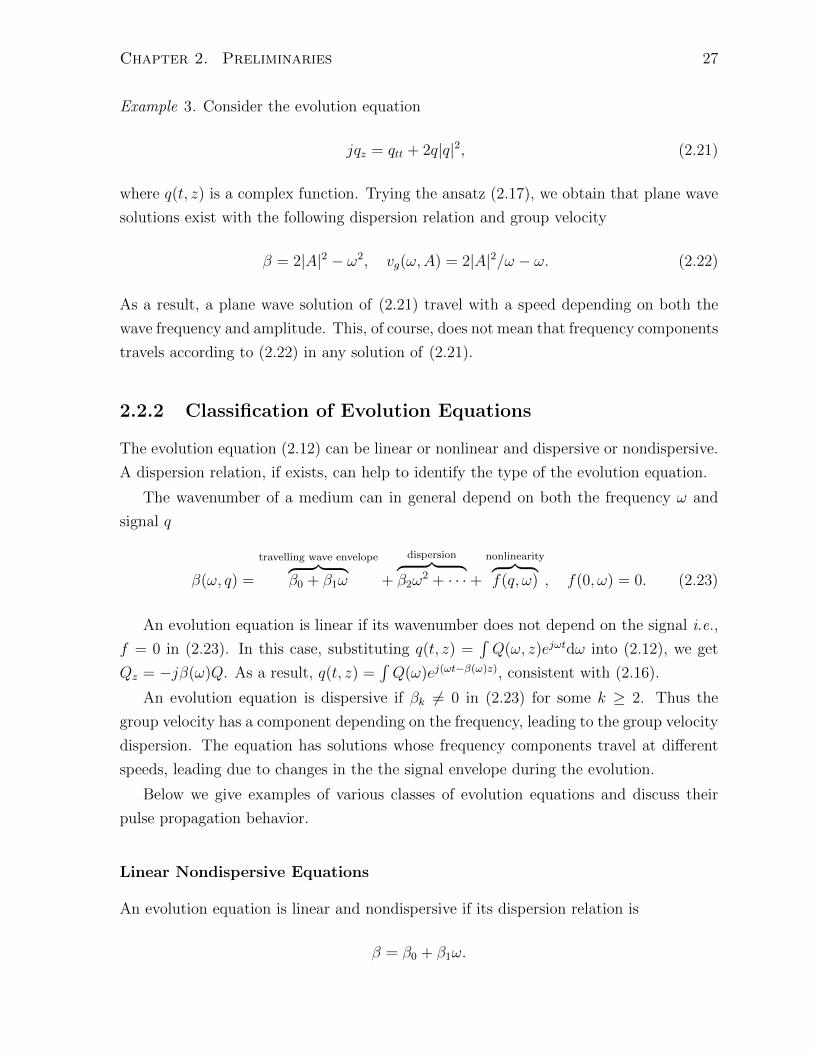
Chapter 2. Preliminaries 27
Example 3. Consider the evolution equation
jqz = qtt + 2q|q|2, (2.21)
where q(t, z) is a complex function. Trying the ansatz (2.17), we obtain that plane wave
solutions exist with the following dispersion relation and group velocity
β = 2|A|2 − ω2, vg(ω,A) = 2|A|2/ω − ω. (2.22)
As a result, a plane wave solution of (2.21) travel with a speed depending on both the
wave frequency and amplitude. This, of course, does not mean that frequency components
travels according to (2.22) in any solution of (2.21).
2.2.2 Classification of Evolution Equations
The evolution equation (2.12) can be linear or nonlinear and dispersive or nondispersive.
A dispersion relation, if exists, can help to identify the type of the evolution equation.
The wavenumber of a medium can in general depend on both the frequency ω and
signal q
β(ω, q) =
travelling wave envelope︷ ︸︸ ︷β0 + β1ω +
dispersion︷ ︸︸ ︷β2ω
2 + · · ·+nonlinearity︷ ︸︸ ︷f(q, ω) , f(0, ω) = 0. (2.23)
An evolution equation is linear if its wavenumber does not depend on the signal i.e.,
f = 0 in (2.23). In this case, substituting q(t, z) =´Q(ω, z)ejωtdω into (2.12), we get
Qz = −jβ(ω)Q. As a result, q(t, z) =´Q(ω)ej(ωt−β(ω)z), consistent with (2.16).
An evolution equation is dispersive if βk 6= 0 in (2.23) for some k ≥ 2. Thus the
group velocity has a component depending on the frequency, leading to the group velocity
dispersion. The equation has solutions whose frequency components travel at different
speeds, leading due to changes in the the signal envelope during the evolution.
Below we give examples of various classes of evolution equations and discuss their
pulse propagation behavior.
Linear Nondispersive Equations
An evolution equation is linear and nondispersive if its dispersion relation is
β = β0 + β1ω.

Chapter 2. Preliminaries 28
In this case, from (2.16) the signal envelope is expressed as the superposition of the
plane waves exp(jω(t− cz)), all traveling with the same speed c = β1. Thus the overall
solution is f(t − cz), where f(t) is the initial data at z = 0. As a result the solution of
linear nondispersive equations are traveling waves, i.e., waveforms that keep their shape,
traveling at a constant speed c (stationary in the co-propagating reference). Fig. 2.7(a)
shows a traveling wave propagating in a linear nondispersive medium.
Example 4 (One-dimensional wave equation in free space). Consider the one-dimensional
wave equation qzz = c2qtt, where q(t, z) represents a wave in time t (e.g., an electromag-
netic field) propagating in the free space in the direction z with velocity c. Plugging in
the plane wave ansatz (2.17), we obtain the dispersion relation
β = ±cω.
As expected, the solution is the sum of the forward and backward traveling waves
(f(t− cz) + g(t+ cz)) /2 and experiences no dispersion.
Linear Dispersive Equations
The dispersion relation of the linear dispersive equations is independent of the signal and
at least quadratic in ω
β(ω) = β0 + β1ω + β2ω2 + · · · ,
where βk 6= 0 for some k ≥ 2.
The dispersion coefficient β2 can be positive or negative. Since the group velocity
dispersion is β2(ω − ω0) to the leading order, high frequencies travel faster than low
frequencies if β2 < 0 or slower if β2 > 0. In both cases, this can lead to pulse broadening
or pulse contraction in the time domain, depending on the input signal1.
Fig. 2.7(b) shows an example of the wave propagation in a dispersive medium when
β2 < 0. Here a pulse initially at z = 0 disperses to zero in the evolution, experiencing
pulse broadening. While the signal energy (and perhaps additional conserved quantities)
can be preserved in a dispersive equation, it can spread over a large time so that locally
the signal energy is negligible in any finite time interval.
1In the frequency domain, a linear system could represent a low pass or a high pass filter, potentiallyleading to spectral broadening or contraction, depending on the definition of the bandwidth (e.g., 99%bandwidth). However spectral broadening in the sense of creation of new frequencies does not occur.See also the footnote in page 44.
Chapter 2. Preliminaries 29
An example of a linear dispersive equation is the heat equation mentioned in Exam-
ple 2. Solving the equation,
q(t, z) = h(t, z)∗ q(t, 0) =
ˆQ(ω, 0)ejω(t−c2ωz)dω, (2.24)
where the impulse h(t, z) is a Gaussian function
h(t, z) =1√
4πc2ze−
t2
4c2z .
It follows that q(t, z) is the sum of the single tone frequencies traveling at speeds propor-
tional to their frequencies. Integral (2.24) is a special case of (2.16).
Nonlinear Nondispersive Equations
Nonlinear nondispersive equations have solutions whose components in time travel with
speeds depending on the signal in that time instance. The shape of the signal generally
changes, but due to the nonlinearity not the dispersion. If the nonlinearity is set to zero,
solutions are traveling waves. If a dispersion relation from a plane wave is obtained, it is
linear in ω and depends on the signal
β = β0 + β1ω + f(A, ω).
Example 5. Consider the following nonlinear equation
qz + αqt + βqqt = 0. (2.25)
The dispersion relation and the group velocity are
β = ω(α + βA), vg = α + βA.
That is to say, samples of the signal with high amplitudes travel faster than those parts
with small amplitudes. Note that a derivative term ∂kq/∂tk contributes to the dispersion
only if k ≥ 2.
In many cases nonlinearity is memoryless and is best understood in the time domain.
Fig. 2.7(c) shows the qualitative features of the pulse propagation in a nonlinear nondis-
persive equation where vq = q, i.e., q(t, z) = q(t − q(t, z)z, 0). The top of the signal
travels faster than the base of the signal, causing the initial pulse to tilt to the right.
Pulse center t = 0 is mapped to a time t′ at z = 1 satisfying q(t′) = t′. It can be verified

Chapter 2. Preliminaries 30
-10-5
05
10 0
1
20
0.5
1|q(t, z)|
tz
|q(t, z)|
-20-10
010 0
12
0
0.5|q(t, z)|
tz
|q(t, z)|
(a) (b)
−4 −2 0 2 40
0.2
0.4
0.6
0.8
1
t
|q(t)|
z = 0z > 0
00
1
20
1
2|q(t, z)|
tz
|q(t, z)|
(c) (d)
Figure 2.7: Wave propagation in a (a) linear nondispersive, (b) linear dispersive, (c)nonlinear nondispersive, and (d) nonlinear dispersive medium.
that (e.g., in the case that z is small), the effect of the signal dependent shift is not
simply titling the pulse, but distorting the waveform.
Example 6. In cases that q(t, z) is complex, signal distortions may occur in the phase of
the signal. Consider the following nonlinear equation
jqz = 2|q|2q. (2.26)
A dispersion relation exists, given by
β = 2|A|2, vg = 2|A|2/ω.
Thus the speed of a single tone frequency depends on the intensity of that component.

Chapter 2. Preliminaries 31
It can be verified that the solution of (2.26) is
q(t, z) = q(t, 0)e2j|q(t,0)|2z.
Although the signal amplitude is preserved during the propagation, its phase is distorted
according to the nonlinearity. There is no dispersion since βk = 0, k ≥ 0, although vg
depends on the frequency as well, due to the nonlinearity.
Nonlinear Dispersive Equations
These equations generally have both elements of the nonlinearity and dispersion in the
wavenumber expansion (2.23).
An example is (2.21), where the equation allows a plane wave solution, and the
resulting wavenumber depends on the signal amplitude and frequency.
Example 7. Consider the nonlinear equation
qz + qttt + qqt = 0.
Unlike Example 2.21, a plane wave solution does not exist. However, it is evident that
by setting the nonlinear term to zero, the equation is dispersive with dispersion relation
β = −ω3.
A nonlinear dispersive equation can be in the anomalous (focusing) or normal (defo-
cusing) regime, depending on the signs of the dispersion and nonlinearity. In the anoma-
lous regime, β2 < 0 and the nonlinearity acts against the pulse broadening effects of the
dispersion ( see Fig. 2.7(d)). In this case, in the frequency domain plot, all frequencies
travel towards the carrier, leading to pulse broadening in time. Since the wavenumber is
a function of the signal intensity as well, if one has a signal whose shape in time is peaked
at the center and decays at other times, like a Gaussian, there is a possibility that the
entire wave packet travels at a constant speed. This corresponds to the formation of a
certain traveling wave packets in the anomalous regime called solitons, similar to that
in Fig. 2.7(a). In the normal regime, β2 > 0 and all frequencies travel away from the
carrier, leading to pulse compression in time. Thus if one has an inverted soliton signal,
there is a possibility of obtaining a traveling wave packet (dark soliton).
Remark 6. Dispersion is best understood in the frequency domain, where its action is
memoryless and multiplicative. The nonlinearity is usually memoryless and multiplica-
tive in the time and is best understood in this domain. Nonlinear dispersive waves are

Chapter 2. Preliminaries 32
TX
HybridAmplifier
Forwardpump
span 1 span 2 span N
SSMF HybridAmplifier
Forwardpump
Backwardpump
ROADM SSMF HybridAmplifier
Forwardpump
Backwardpump
ROADM SSMF HybridAmplifier
Backwardpump
RX
Figure 2.8: Fiber-optic communication system.
challenging to analyze because the degrees of freedom are coupled both in time and fre-
quency. These equations often do not take simple forms in either time or usual frequency
domains.
2.3 Lightwave Communications
The amount of information that can be transmitted on a signal is proportional to the
carrier frequency (bandwidth ∼ carrier frequency). With the introduction of lasers in
1960s, it was speculated that a shift from the radio and microwave spectrum to optical
frequencies near the infrared spectrum can significantly increase data rates. At wave-
lengths close to the visible light wavelengths, elements of the atmosphere contribute to
a significant signal loss and random refractive index. This makes transmission of light-
waves over long distances in the exposed atmosphere nearly impractical. In search for a
medium for the newly invented laser, optical fiber was suggested in 1966 [18].
Early fibers had significant loss and low-loss fibers were not made available until the
1970s. Fiber-optic communication systems initially used expensive repeaters in the 1980s
to regenerate the signal. The advent of the optical amplifiers in 1987 [19, 20] and the
wavelength-division multiplexing in mid 1990s subsequently revolutionized the fiber-optic
communications.
Fig. 2.8 shows the block diagram of a typical optical communications system. Im-
portant components of such a system include laser sources, optical modulators, fiber
segments, amplifiers, reconfigurable add-drop multiplexers (ROADMs), filters, and de-
modulators.
A laser source generates a coherent beam of light which is then modulated by the
optical modulator. The transmitted signal is amplified in a lumped or distributed manner
to keep the signal level constant over a fiber segment. At the receiver, a coherent detector
measures signal quadratures of the channel of interest, which are subsequently used
for the statistical detection. An important element in WDM optical fiber networks is

Chapter 2. Preliminaries 33
the ROADM. In these networks a fiber link has to be shared among many users, each
operating at a distinct wavelength. The signals of the users are added or dropped by
ROADMs. A WDM signal may be accessible at the transmitter only, receiver only,
both or neither one. In the later case the signal enters and leaves the fiber link in an
intermediate distance without even being noticed by the transmitter or the receiver.
Below, we very briefly explain the function of the components of the Fig. 2.8.
2.3.1 Components of a Fiber-optic System
Optical Fiber
Optical fiber used in the long-haul communications consists of a cylindrical core sur-
rounded by a cladding, both usually made of the silica glass SiO2. Silica glass has
numerous desirable transmission, environmental, and mechanical properties, making it
perfect for data communications. The fiber glass is so transparent that today it can be
manufactured to carry a laser signal more than 15 km while maintaining half of its power.
Lightwave communications systems have bandwidths of the order of THz, ideal for the
core networking applications. Silica glass is as strong as steel and can be fabricated in
µm diameters with high precision, and yet remarkably sturdy and flexible. It is hard to
imagine a medium better suited to high data rate transmission than optical fiber.
In the communication systems considered in this thesis, the typical launched powers
correspond to a large number of photons, and the classical theory of Maxwell equations
would suffice to describe the light propagation, instead of the quantum mechanics. Indeed
light transmission in optical fibers can be qualitatively explained via the total internal
reflection phenomenon in geometric optics: the silica glass is doped to shape the refractive
index so that the refractive index of the fiber core is higher than that of the cladding,
either in a step wise manner or smoothly. If the angle of the incidental ray with the
fiber axis is smaller than a critical angle, the total internal reflection occurs in the core
cladding surface, confining the light inside the fiber [21].
In the following, we review two important parameters of the optical fiber.
Fiber Loss Until the 1970s, the fiber loss was so substantial (α > 20 dB/km) that
a lightwave signal could not be sent in the fiber more than a few kilometers. Traces of
OH ions and heavy metal impurities left in the silica glass can contribute to a significant
loss. Fig. 2.9 shows the graph of the fiber loss versus wavelength. Causes of the loss
are either intrinsic, due to the infrared (7.4µm < λ < 300µm) and ultraviolet (10 nm <
λ < 0.4 µm) absorptions occurring in the fused silica, or extrinsic due to impurities.

Chapter 2. Preliminaries 34
Dis
pers
ion
(ps/
nm.k
m)
0.1
0.2
0.3
0.4
0.5
0.6
Atte
nuat
ion
(dB
/km
)
1100 1200 1300 1400 1500 1600 1700
Wavelength (nm)
DSF
20
EDFA bandNZDSF
Attenuation(all fiber types)
10
0
–10
–20
17
3–8
0
Standardsinglemode fiber
Figure 2.9: Fiber loss and dispersion versus wavelength (Courtesy of [1]).
A significant source of loss is the OH ions from water vapors left in the glass, whose
harmonics contribute to the peak of the Fig. 2.9. At a wavelength close to λ = 1.55 µm
loss has a minimum of about 0.2 dB /km.
To compensate for the power loss, fiber-optic communications systems use optical
amplifiers. However, as we will see, these amplifiers introduce noise into the system.
Thus one can trade perturbations caused by the loss with the fluctuations caused by the
amplifiers.
Chromatic Dispersion As noted in Section 2.2.1, the dispersion (wavenumber) of a
medium is generally frequency dependent. The first coefficient β1 is a constant term in
the speed and can be removed by introducing a retarded time. The second coefficient
β2 [sec2/km] gives rise to the velocity of the envelope (2.20) and is called the dispersion
coefficient. In the context of the optical fiber, it is often convenient to express β2 in terms
of the dispersion parameter
D = −2πc
λ20
β2 ps/(nm.km),
where c is the speed of light and λ0 is the carrier wavelength. That is to say, in analogy
with a horse race, there is a delay of D picoseconds after 1 km between two wavelengths
of 1 nm apart. Positive and negative D correspond, respectively, to the anomalous
(focusing) and normal (defocusing) regimes.
Fig. 2.9 shows the graph of the dispersion versus wavelength for a standard single

Chapter 2. Preliminaries 35
mode fiber. In addition to the coefficient β2,, usually the third-order coefficient β3 is also
specified by the fiber manufacturers, expressed in terms of the dispersion slope
S =dD
dλ=
4πcβ2
λ3−(
2πc
λ2
)2
β3.
The amount of the pulse broadening as a result of the dispersion is roughly DL∆λ,
where ∆λ is the wavelength resolution set by the laser spectral width [21]. For a standard
single mode fiber with D = 17 ps/(nm.km), and a laser source with ∆λ = 0.1 nm (i.e.,
∆f ≈ 12.5 GHz), the amount of the pulse broadening is 1700 ps in 1000 km, an ISI of
∼ 21 symbols for pulses with ∼ 80 ps duration.
To suppress the effects of the dispersion, optical or electrical dispersion management
(DM) is used. In optical dispersion management, segments of the fiber with positive and
negative dispersion are used in cascade so that the signal is confined to its initial time
window. In the electrical dispersion management, dispersion is compensated using digital
signal processing at the transmitter, receiver or both. It has been demonstrated that
optical systems greatly benefit from dispersion management in several ways. However,
although the effects of the dispersion can be removed in the frequency domain, dispersion
is coupled to the nonlinearity, and performing DM does not alleviate the impacts of the
nonlinearity.
The wavenumber β(ω), loss coefficient α(ω), refractive index n(ω), and material rel-
ative permittivity εr(ω,E) can all be obtained from the susceptibility parameter χ
n(ω,E) = 1 +1
2<χ(ω,E),
β(ω,E) = ωn(ω,E)/c,
α(ω) =ω
nc=χ(ω, 0),
εr(ω,E) = 1 + χ(ω,E),
where E is the electric field.
Optical Amplifiers
Optical amplifiers work as a result of the process of the stimulated emission, occurring
e.g., in a p−n junction, due to the interaction of the light with matter. The same process
also underlies the operation of the lasers, transistors, diodes, and integrated circuits.
Consider an n-type semiconductor, having excess electrons in the conduction band
with excited state energy E2, in contact with a p-type semiconductor, having holes in

Chapter 2. Preliminaries 36
hω
E2
E1
hω
hω
hω
E2
E1
(a) (b)
Figure 2.10: (a) Spontaneous emission. (b) Stimulated emission.
the valance band with ground state energy E1. The p− n junction is forward biased to
reduce the width of the built-in voltage and establish a current. When an electron is
absorbed from the excited state E2 in a nearby hole at the lower state E1, a photon with
the frequency ω = (E2 − E1)/h is emitted. This can happen either spontaneously, in
which photons are emitted with no external trigger and in random phases and directions,
or stimulated by an external light source with frequency ω = (E2 − E1)/h, in which
the emitted photons are identical in phase, frequency and direction with the external
photons.
Since in the stimulated emission the external and emitted photons are coherent, op-
tical amplification can be realized. The amplification can be done in a discrete manner
at several locations in the optical link using the erbium-doped fiber amplifiers (EDFAs)
or continuously along the fiber using the Raman amplification.
Erbium-doped fiber amplifiers An EDFA consists of a short piece of fiber (a few
tens of meters) doped with erbium ions or a similar dopant and optically pumped at
1.48 µm or 0.98 µm. While the amplification is achieved via the stimulated emission,
some erbium ions move from the excited state to the ground state “spontaneously” as
well, giving rise to the amplified spontaneous emission (ASE) noise.
The input output relationships of the signal before and after an EDFA located at
distance z is
q(t, z+) = Gq(t, z−) + V (t)
where G = eαLsp is the amplifier gain in a span of fiber with length Lsp and loss coefficient
α and V (t) is the ASE noise. It has been demonstrated that the ASE noise is well modeled
as additive white Gaussian with the power spectral density [22]
PSD = nsphω0(G− 1). (2.27)
Here nsp ≥ 1 is the spontaneous emission efficiency factor, h is the Planck’s constant, ω0

Chapter 2. Preliminaries 37
Table 2.1: Fiber Parameters.nsp 1 spontaneous emission factor
h 6.626× 10⁻³⁴J · s Planck’s constant
ω0 193.55 THz carrier frequency
α 0.046 km−1fiber loss (0.2 dB/km)
γ 1.27 W−1km−1nonlinearity parameter
is the optical carrier frequency, and G is the amplifier gain. Typical fiber parameters are
given in Table 2.1.
The efficiency of an EDFA is usually described by its noise figure, defined as the ratio
of the SNRs at the amplifier input and output. It can be shown that
NF = 2nsp −1
G(2nsp − 1) < 2nsp.
When G 1, NF ≈ 2nsp and the noise figure becomes a measure of nsp. In general
NF ≥ 0 dB , and for amplifiers where G 1 and nsp = 1, NF ≈ 3 dB .
The graph of the gain of an EDFA versus wavelength is peaked around 1.53 µm, and
maintains a large gain in the optical C band 1.53 µm ≤ λ ≤ 1.565 µm (a window of
35 nm). Thus EDFAs can conveniently operate near the 1.55 µm system wavelength,
where the fiber loss is minimum. The EDFA gain depends on the pumped power and
can be as high as 30 − 50 dB , with a noise figure NF ≈ 3 − 5 dB and output power
10− 25 dBm.
Raman amplification In the distributed Raman amplification, the fiber itself, without
doping, is used as a gain medium. Amplification is achieved thorough the process of
stimulated Raman scattering (SRS). Raman pump units, placed at several locations in
the optical link, inject high power fields in forward and backward directions. The incident
field at frequency ωin is absorbed by the silica glass, turning electrons in silica into
oscillating dipoles, which in turn emit light at a lower frequency ω < ωin. As before, the
scattering process can be stimulated by an external light source of frequency ω, giving
rise to distributed optical amplification . This keeps the signal power slightly varying
around a constant mean along the fiber. The resulting ASE noise is Gaussian and white
in space time
EN(t, z)N∗(t′, z′) = σ20δ(t− t′, z − z′).
The noise power spectral density is obtained by taking the limit Lsp → 0 of (2.27),
obtaining
σ20 = nsphω0αL,

Chapter 2. Preliminaries 38
where L is the total fiber length. The graph of the Raman gain versus frequency has a
peak around 13.2 THz with a broad bandwidth as large as 8 THz. The pumped fields
have high powers of a few watts, making the commercial development of distributed
amplification challenging.
Optical Lasers
The optical source in long-haul high data rate systems is typically a semiconductor laser.
A laser source is essentially an optical amplifier, operating based on the same principle
of the stimulated emission, together with a feedback mechanism, to produce a powerful
coherent beam of light. The output of a semiconductor laser source used in optical com-
munications can have powers typically as high as few hundred milliwatts, concentrated
around the signal frequency with a small linewidth (laser ∆f before modulator due to
phase noise, typically of order of MHz). We ignore the effects of the laser ASE noise and
the non-zero laser linewidth in this thesis.
The bandwidth of a lightwave communications system, while depending on the band-
width of all system components such as the laser source, fiber, amplifiers and network
equipments, is usually limited by the bandwidth of the electronic circuits at the receiver.
2.3.2 Simplified Derivation of the NLS Equation
Derivation of the pulse propagation equation in optical fibers may be found in the stan-
dard text [21] or published papers. It is however useful to sketch a simplified derivation
here to see the essence of the various terms in our channel model.
As mentioned earlier, pulse propagation in optical fibers is described by the classical
theory of Maxwell equations. Canceling the magnetic fields in these equations, we obtain
the well-known wave equation in the frequency domain
∇×∇× E = −µ0ω2D, (2.28)
where E and D are the electric field and displacement vectors, µ0 and ε0 are, respectively,
vacuum permittivity and permeability, and the hat symboldenotes the operation of the
Fourier transform.
The displacement vector D depends on E. Expanding D in terms of E in a vector

Chapter 2. Preliminaries 39
Volterra series (like a Taylor expansion for functionals)
D = ε0
∞
−∞
ε(1)r (τ)E(t− τ)dτ
+
∞
−∞
∞
−∞
∞
−∞
ε(3)r (τ1, τ2, τ3) : E(t− τ1)E(t− τ2)E(t− τ2)dτ1τ2τ3 + · · · , (2.29)
where ε(k)r (τ1, · · · , τk) is the kth-order permittivity kernel and following the inversion
symmetry (centro-symmetry) of the SIO2 crystal, the second-order kernel is zero. The
notation εkr : E · · ·E means a 3×1 vector whose each component is a product Ei1 · · ·Eik ,1 ≤ i1, · · · , ik ≤ 6, capturing interactions between the x, y, z components of the electric
field and its conjugate at all times. For k = 1, the kernel ε1r is simply a 3× 3 matrix.
Assuming an isotropic wave propagation and ignoring the polarization birefringence,
the tensors are diagonal and the wave propagation in each spatial coordinate is described
independently by a scalar equation. The vector Volterra series (2.29) then reduces to a
scalar Volterra series for each component, e.g., D := D.x and E := E.x
D = ε0
∞
−∞
ε(1)r (τ)E(t− τ)dτ
+
∞
−∞
∞
−∞
∞
−∞
ε(3)r (τ1, τ2, τ3)E(t− τ1)E∗(t− τ2)E(t− τ2)dτ1τ2τ3 + · · · . (2.30)
We remove the carrier exp(j(ω − ω0)t) and assume that the envelope is slowly-
varying so that the kernel ε(3)r (τ1, τ2, τ3) appears to be a delta function ε
(3)r (τ1, τ2, τ3) =
ε(3)r δ(τ1, τ2, τ3) with a constant coefficient ε
(3)r . This simplifies the nonlinear term to
ε(3)r |E(t)|2E(t). We then take the Fourier transform of the resulting equation. Given the
small perturbative nature of the nonlinearity, we further assume that |E(t)|2 is almost
constant, so that E3(ω) ≈ |E|2E(ω). As a result, in the frequency domain we obtain the
simple relation D = ε0εrE, where
εr(ω, |E|2) = ε(1)r (ω) + ε(3)
r |E|2. (2.31)
The wave equation (2.28) can be solved under (2.31). Assuming the separation of
variables, we can express components of the envelope of E as F (x, y)q(z, t) exp(j(ω0t −β0z)). The cross section function F is separated out as in the linear cases. The space

Chapter 2. Preliminaries 40
derivatives ∂/∂x2 + ∂/∂y2 from ∇×∇×E give F in terms of the Bessel functions. The
second derivative of the remaining term q(z, t) exp(j(ω0t − β0z)) involves qzz, qz and q.
For the slowly varying function q (in z), the curvature qzz is ignored, and we obtain a
dispersion relation for q
β(ω, |q|) = β0 + β1(ω − ω0) +1
2β2(ω − ω0)2 + · · ·+ γ|q|2, (2.32)
where γ = ω0n2/(cAeff ) is the Kerr nonlinearity coefficient and n2 is the refractive index.
The constant factor Aeff is the effective cross section and depends on F (x, y) [21]. The
terms β − β0 and (ω− ω0)k in the frequency represent, respectively, −jα/2− j∂/∂z and
and j∂/∂t in the time. Multiplying (2.32) by q and making these substitutions, we obtain
the nonlinear Schrodinger equation
qz +α
2q + β1qt +
jβ2
2qtt = jγ|q|2q.
Note that the NLS equation is valid under the following assumptions:
• Signal bandwidth is much smaller than the carrier so that the higher order terms
(ω−ω0)k in the dispersion expansion are negligible at some k. This corresponds to
a slowly varying envelope and is generally valid for pulses with duration T > 1ps.
• The medium is weakly nonlinear so that the cubic nonlinearity is a perturbation
around the linear dispersion and the higher order nonlinear terms are negligible.
• The signal power is not too large so that other nonlinear phenomena, such as
certain scattering processes not discussed here, can be ignored.
The NLS equation has been tested and used for many years now and it generally
describes the experimental results very well.
Remark 7. Dispersion is due to the memory property of a dielectric and is reflected in
the fact p(t) depends on E(t) in past and future, in the form of a convolution. This
memory in turn, through the wave equation, implies nonuniform speeds across frequen-
cies. Nonlinearity on the other hand is largely instantaneous, due to the dependency of
the susceptibility to the intensity of the light.
Remark 8. Note that although the nonlinearity is locally a small perturbation around
the dispersion, its effects are gradually accumulated with z.

Chapter 2. Preliminaries 41
2.4 Summary
Due to the inter-disciplinary subject of this thesis, we provided some of the necessary
background in information theory, evolution equations and fiber-optic communications
for the audience not familiar with some of these areas. Further details may be found in
references made throughout this chapter.

Chapter 3
Origin of Capacity Limitations in
Fiber-optic Networks
It is a capital mistake to theorize
before one has data.
Sir Arthur Conan Doyle, A Study in
Scarlet.
Recent studies on the information capacity of WDM optical fiber networks suggest
that the spectral efficiency of such networks is ultimately limited by the inter-channel and
intra-channel nonlinear interactions [7]. These interference distortions are deterministic
and signal-dependent stochastic effects and grow with the input signal power, diminishing
the capacity and the spectral efficiency at high signal-to-noise ratios. In these studies,
the capacity, C, increases with input power power, P , reaching a peak at a certain critical
input power, and then asymptotically vanishes as P → ∞ (see e.g., [7] and references
therein).
In this chapter, we briefly review the WDM model that is commonly used in these
studies, as well as in the practical optical fiber systems. We briefly identify the origin
of the capacity limitations in this model and explain that this method and similar ones,
which are borrowed from linear system theories, are inappropriate for the communication
over optical fiber networks. In particular the limitation of the capacity in the prior
work is an artifact of these methods and some of the factors commonly believed to
limit the achievable information rates are not indeed fundamental. In the subsequent
chapters, we present a method that is able to fix these limitations and is fundamentally
compatible with the structure of the nonlinear fiber optic channel, promising a higher
spectral efficiency that keeps increasing beyond the critical input signal power associated
42

Chapter 3. Origin of Capacity Limitations in Fiber-optic Networks 43
with linear transmission methods.
3.1 Capacity of WDM Optical Fiber Networks
Fiber-optic communication systems use wavelength-division multiplexing to transmit in-
formation. Similar to frequency-division multiplexing (FDM), in this method information
is multiplexed in distinct wavelengths. This helps to separate the signal of the indepen-
dent users in a network, where they have to share the same links between different nodes
of the network.
Fig. 3.1 shows the system model for the part of an optical fiber network between
a source and a destination. There are N fiber spans between multiple users at the
transmitter (TX) and multiple users at the receiver (RX). The signal of some of these
users is destined to a receiver other than the RX shown in Fig.3.1. As a result, at the
end of each span there is a ROADM that may drop the signal of the some of the users
or, if there are free frequency bands, add the signal of the potential external users. We
are interested in evaluating the spectral efficiency of the fiber link from the TX to the
RX.
Recall that the propagation of the complex envelope of a narrowband signal in each
span of the fiber with distributed amplification is described by the stochastic nonlinear
Schrodinger (NLS) equation [21,23]
∂Q(τ, `)
∂`+jβ2
2
∂2Q(τ, `)
∂τ 2= jγQ(τ, `)|Q(τ, `)|2 + V (τ, `), 0 ≤ ` ≤< L. (3.1)
Here ` denotes distance (in km) along the fiber; the transmitter is located at ` = 0,
and the receiver is located at ` = L = NLsp. The symbol τ represents retarded time,
measured in seconds, i.e., τ = t− β1` where t is ordinary time and β1 is a constant, and
Q(τ, `) is the complex envelope of the signal propagating in the fiber. The coefficient β2,
measured in s2/km, is called the chromatic dispersion coefficient, while γ, measured in
W−1km−1, is the nonlinearity parameter. Finally, V (τ, `) is bandlimited white Gaussian
noise with in-band spectral density σ20 (W/(km · Hz)) and autocorrelation
E V (τ, `)V ∗(τ ′, `′) = σ20δW (τ − τ ′)δ(`− `′),
where δW (x) = 2W sinc(2Wx). It is assumed that the transmitter is bandlimited to W

Chapter 3. Origin of Capacity Limitations in Fiber-optic Networks 44
for all `, 0 ≤ ` ≤ L, and power limited to P0
E1
T
ˆ T0
|Q0(t)|2dt = P0.
The stochastic NLS equation (3.1) models both chromatic dispersion (captured by
the jβ2∂2Q/∂τ 2 term), which is responsible for temporal broadening, and the Kerr non-
linearity (captured by the γ|Q|2Q term), which is responsible for spectral broadening.
Pulse propagation is governed by the tension between these effects and can be linearly
dominated, nonlinearly dominated, or solitonic (in which case the two effects are bal-
anced).1 The NLS equation defines a nonlinear dispersive waveform channel from Q(τ, 0)
at the transmitter to Q(τ,L) at the receiver.
We will find it convenient to work with the nonlinear Schrodinger equation (3.1) in a
normalized form. By changing variables
q =Q√P, z =
l
L , t =τ
T0
, (3.2)
with T0 =√|β2|L
2and P = 2
γL , we get the normalized stochastic NLS equation
jqz(t, z) = qtt + 2|q(t, z)|2q(t, z) + v(t, z), (3.3)
where
E v(t, z)v∗(t′, z′) =σ2
0
PT0
δW (t− t′)δ(z − z′).
Throughout this thesis, we primarily work with the normalized equation (3.3).
Stochastic partial differential equations (SPDEs) are usually interpreted via their
equivalent integral representations. Integrating a function with unbounded variation is
problematic, since e.g., a Riemann approximation´ z+dz
zg(z)dB(z) ≈ g(l)(B(z + dz) −
B(z)), l ∈ [z, z + dz], where B is the Wiener process, would depend on the choice of l
1The action of a linear time-invariant system in the frequency domain is a multiplication by a fil-ter H. This gives rise to separate amplitude and phase relations between input X and output Y(e.g., |Y | = |X||H|). In contrast, the cubic nonlinearity in (3.3) is a triple convolution in the fre-quency domain, i.e., an integral in which spectrum samples at various frequencies are (vectorially)added up with different angles (phases) controlled by dispersion. It follows that the nonlinearity con-verts phase modulations made by the dispersion to the amplitude modulations, leading to a constantexchange of information between amplitude and phase during the evolution. As a result, although theall-pass dispersion filter in (3.3) individually does not lead to any spectral broadening or narrowing,in the presence of a nonlinearity it can lead to such effects, thereby countering or amplifying the ef-fects of the nonlinearity. The interaction between nonlinearity and dispersion can be understood viaq(t, z) = e−jz∂ttq(t, 0)− j
´ z0e−j(z−z
′)∂tt(2|q(t, z′)|2q(t, z′) + v(t, z′)
)dz′, or its simplified (frequency do-
main) version (3.6).

Chapter 3. Origin of Capacity Limitations in Fiber-optic Networks 45
(this ultimately comes from the linearity of variance stated in Observation 1). This leads
to various interpretations for a SPDE, notably Ito and Stratonovich representations in
which, respectively, l = z and l = z + dz/2 [24]. Due to conclusions made in this work,
noise is treated only briefly in Section 6.5, where these conventions do not influence
our results. Note that in the case that noise is bandlimited in time, the stochastic
PDE is essentially a finite dimensional system and there is no difficulty in the rigorous
interpretation of the stochastic NLS equation.
In a WDM optical system, the following signal is transmitted over the channel
q(t, 0) =N∑
k=1
(WT∑
l=1
slkφl(t)
)ejk2πWt, 0 ≤ t ≤ T, (3.4)
where sk are the transmitted symbols, φl(t) are pulse shapes, W ≥ 1/T is the per
channel bandwidth and N is the number of WDM channels. For illustration pur-
pose, we can assume that each user sends an isolated pulse in the time interval [0, T ].
Thus each user operates at a single frequency in a bandwidth W = 1/T and q(t, 0) =∑N1 qk(0) exp(jk2πt/T ), where qk(0) are the Fourier series coefficients at z = 0. When
this signal is subject to an evolution, we have a Fourier series with variable coefficients
q(t, z) =N∑
k=1
qk(z)ejk2πtT . (3.5)
Substituting the periodic solution (3.5) into (3.1), we get the NLS equation in the
discrete frequency domain
j∂qk(z)
∂z= −4π2W 2k2qk(z)︸ ︷︷ ︸
dispersion
+ 2|qk(z)|2qk(z)︸ ︷︷ ︸SPM
+ 2qk(z)∑
l 6=k|ql(z)|2
︸ ︷︷ ︸XPM
+ 2∑
m6=kl 6=k
qm(z)ql(z)q∗m+l−k(z)
︸ ︷︷ ︸FWM
+vk(z), (3.6)
in which vk are the noise coordinates in frequency and we have identified the disper-
sion, self-phase modulation (SPM), cross-phase modulation (XPM) and four-wave mixing
(FWM) terms in the frequency domain.
It is important to note that the optical WDM channel model is a (nonlinear) multi-

Chapter 3. Origin of Capacity Limitations in Fiber-optic Networks 46
user interference channel [25]. The (inter-channel) interference terms are the XPM and
FWM. There is no inter-symbol interference (ISI) in the isolated pulse transmission
model (3.6) with one degree of freedom per user. However in a pulse train transmission
model where WT > 1, replacing qk by sk via the inverse transform shows that the
other two effects, the dispersion and SPM, cause inter-symbol interference (intra-channel
interaction). Performance of a WDM transmission system depends on how interference
and ISI are treated, and in particular the availability of the interference signals at the
receiver. Several cases can be considered.
The SPM term of each user is available at the receiver for that user. Its deterministic
part, if needed, can be removed, e.g., by back propagation and its (signal-dependent)
stochastic effects are handled by coding and optimal detection over a long block of data
(e.g., maximum likelihood sequence detection). ISI is therefore not a limitation to the
capacity.
In contrast, a serious limitation to the capacity of optical fiber networks is the inter-
channel interference. In optical fiber networks many users have to share the same optical
fiber link. Each user has access to the signal in its own frequency band, and the signal of
the users ql, l 6= k, is generally unknown to the kth user. In linear Gaussian channels there
is no interference between users operating in disjoint frequency bands. In a nonlinear
channel where, by definition, additively is not preserved under the action of the channel,
multiplexing signals in a linear fashion, e.g., by adding them in time or in frequency,
leads to inter-channel interference.
In WDM optical systems, such linear frequency multiplexing is performed in ROADMs
located in several locations throughout the fiber link. If multiplexing and demultiplexing
is done only at the transmitter and receiver, one has access to the XPM and FWM
interference terms. In this case interference is handled optimally by joint transmission
and statistical detection, e.g., using multiuser detection techniques. Such channel is
essentially akin to a single user channel. Here one is expected to get an overall capacity
similar to that of linear systems by joint transmission and detection.
Unfortunately in optical fiber networks it is not generally possible to perform joint
transmission and detection. Many signals join and leave the optical link in intermediate
distances without even being noticed by any user, leaving behind a residual nonlinear
impact. The interference resulting from these signals is unavoidably treated as noise and
ultimately limits the capacity of optical fiber networks.
Assuming the coefficients qk(z) remain independent in (3.6) during the evolution, the
Chapter 3. Origin of Capacity Limitations in Fiber-optic Networks 47
XPM term is statistically regulated as N →∞∑
l 6=k|ql(z)|2 → N − 1
NP0 → P0.
Thus the XPM does not influence the capacity of optical fibers significantly. The FWM
on the other hand is cubic in signal and is not averaged out as XPM [26]. It is obvious that
this interference will explode when increasing the common average power P , ultimately
overwhelming the signal and reducing the capacity to zero. The per degree of freedom
capacity versus power curve C(P) is noise-limited in low SNRs following log(1 + SNR )
and interference-limited in high SNRs, decreasing to zero [7, 26,27]; see Fig. 3.2.
It follows that the information capacity of the nonlinear Schrodinger channel depends
on the model assumed on this equation. One can assume a single-user or multiple-user
channel with or without memory modeling. Below, we briefly elaborate on each case,
essentially repeating the above argument.
Single-user discrete channels Capacity (bits/channel use) of a single user discrete
channel (one complex degree of freedom) is a concave and non-decreasing function of
the input average power (equality- or inequality-constraint). For a discrete memoryless
channel this follows from the concavity of the mutual information as a function of the
input distribution and the linearity of the cost constraint [28]. This, of course, holds true
for any set of transition probabilities, including that obtained from nonlinear channels.
Consider for instance the nonlinear channel
Y = X +X2N, EX2 = P ,
where random variables X, Y and N are, respectively, input, output, and noise. The
power of the signal dependent additive noise term X2N increases at a faster rate com-
pared to the power of the signal term X. This, however, does not mean that the signal-
dependent noise diminishes the capacity at high powers. In Shannon’s argument, one is
only concerned with typical sequences, in which the “good” and “bad” input symbols are
averaged out. Nontypical sequences such as (x1, · · · , x1) may have variable output “noise
balls”, potentially large and increasing with x1, but the noise balls associated with all
input typical sequences have the same size in the sphere packing picture. In this sense,
there is no distinction between linear and nonlinear channels when they are extended in
time.

Chapter 3. Origin of Capacity Limitations in Fiber-optic Networks 48
ISI in channels with memory Capacity of a single-user waveform channel is mea-
sured in bits per degree of freedom (equivalent to bits/s/Hz). Sending a large sinc
wavetrain, as in (3.4) with N = 1, over the stochastic NLS equation, performing back
propagation and maximum likelihood sequence detection at the receiver, one is expected
to obtain a capacity that is nondecreasing with average input power. Thus the determin-
istic or stochastic intra-channel effects do not limit the capacity when joint transmission
and detection of the degrees of freedom in time is computationally feasible. However
assuming a discrete memoryless model for a nonlinear channel with memory such as the
optical fiber, as often done in the literature, can potentially limit the capacity. This is
explained below.
Note that, while the ISI is deterministic in traditional linear channels, for a nonlinear
waveform channel, ISI can have a stochastic component as well. Even if a deterministic
channel is a set of parallel non-interacting channels, noise addition, which usually becomes
signal-dependent in the presence of a nonlinearity, can correlate these channels and bring
the interference signals to the location of the channel of interest. Just as deterministic
interference, this stochastic interference can limit the capacity of a nonlinear channel.
This occurs only if the projection of the noise on the induced degrees-of-freedom is
signal-dependent.
As a result if one sends the wavetrain (3.4) over the NLS channel and performs back
propagation over the entire received block of data to remove the deterministic ISI, a net
signal dependent noise is left over for each symbol
srl = sil + f(si1, · · · , siWT , v), l = 1, · · · ,WT,
where sil and srl are transmitted and received symbols and v is the noise. It is clear that
performing isolated symbol detection, e.g., per-symbol nearest neighbor mapping, has a
capacity vanishing at high powers. This is in contrast to the application of the OFDM
to linear ISI channels. The C(P) curve is, of course, similar to that of the linear systems
if a maximum likelihood sequence detector (MLSD) is employed in which the sequence
(si1, · · · , siWT ) is jointly detected. The gains of using a MLSD are thus more pronounced
in the nonlinear optical channel where the isolated detection poses a severe limitation to
the capacity.
Interference in multi-user channels Here we are interested in the per user capacity
and the sum rate of the multi-user channel. The per degree of freedom capacity of a
continuous or discrete multi-user channel can potentially be decreasing with common
Chapter 3. Origin of Capacity Limitations in Fiber-optic Networks 49
average power P if users interfere with one another and do not cooperate to manage this
inter-channel interference. This can be an issue for linear channels as well; it is just a
more serious issue for a strongly nonlinear channel such as the cubic NLS channel. The
inter-channel interference is just the dual of the intra-channel ISI; the only difference
is that cooperation and joint transmission and detection may not be physically possible
among users. With users cooperating, one expects a nondecreasing per degree of freedom
capacity similar to that of the linear systems. As we will see in this thesis, sometimes
it is also possible to identify a set of non-interacting degrees-of-freedom for a nonlinear
channel, giving rise to a transmission scheme in which the inter-channel interference does
not limit the capacity.
Spectral broadening in nonlinear channels When a signal propagates in a nonlin-
ear evolution equation, its spectrum can spread continuously. The amount of spectrum
broadening depends on the pulse shape and generally is proportional to the signal power.
While bits/symbol may increase with power, bit/sec/Hz may asymptotically vanish. Here
we should divide bits/symbol to the maximum signal dimensions that admissible input
signals occupy during the entire evolution. Spectral broadening is a serious issue in zero-
dispersion fibers where the channel is strongly nonlinear [29]. In dispersive channels,
it has been observed that pseudo-linear transmission does not suffer from a significant
spectral broadening and this effect is not as significant [7]. Here one can simply divide
the capacity by input bandwidth to obtain spectral efficiency.
3.2 The Importance of the Inter-channel Interfer-
ence
From the above discussion it follows that while the intra-channel interference can be
handled by memory modeling, the inter-channel interference ultimately limits the capac-
ity of optical fiber networks. The current practice in fiber-optic communications is to
send a linear sum of signals in time (pulse train) and in frequency (wavelength-division
multiplexing) in the form of (3.4), both of which are poor ideas for the nonlinear fiber
channel. Thus we identify ROADMs as the main culprit for the capacity limitation in
optical fiber networks. These devices perform linear multiplexing of signals which is not
consistent with the structure of the NLS equation, resulting in a severe interference that
is subsequently treated as noise. A modification of these devices is needed so that the
incoming signals are multiplexed in a nonlinear fashion, exciting noninteracting degrees

Chapter 3. Origin of Capacity Limitations in Fiber-optic Networks 50
of freedom of the NLS equation. Note that the noise or intra-channel effects are not
the primary reasons for the limitations of the capacity in the optical fiber networks and
cannot bring down the C(P) curve.
The effect of the interference when using the traditional frequency-division multiplex-
ing in the nonlinear fiber channel is shown in Figs. 3.1 and 3.2. Here we have simulated
transmission of 5 WDM channels over 2000 km of standard single-mode fiber with 100
spans. At the end of each span, a ROADM filters the channel of interest (COI) in the
middle at 40 GHz bandwidth, and adds four side-band signals randomly from a common
constellation (brown curves). At the output, the COI is filtered and back-propagated
according to the inverse NLS equation. It can be seen that the nonlinear inter-channel
interference is stronger at higher powers. Since this simulation is performed for isolated
pulses per channel due to speed considerations, the per-channel power is increased by
a factor of 5 to mimic the high energy nature of the pulse trains. Under a pulse train
transmission, inter-channel interference effects are more significant.
It is clear from the Figs. 3.1-3.2 that as the average transmitted power is increased,
the signal-to-noise ratio in the COI, and as a result the information rate, vanishes to
zero. Note that this effect can simply be described by a SNR analysis at the receiver and
one does not need a sophisticated information-theoretic analysis to illustrate it, unless
exact numbers for the spectral efficiency are of interest. As it can seen from Fig. 3.1, the
quality of the received signal in the COI degrades with power and taking the logarithm
of the SNR gives the intended result fairly closely. The degradation of the capacity is
simply because the real SNR is actually lower than the perceived SNR .
In the subsequent chapters it is shown that it is possible to exploit the integrability of
the nonlinear Schrodinger equation and induce a k-user interference channel on the NLS
equation so that both the deterministic inter-channel and inter-symbol interferences are
zero for all users. This is done using the nonlinear Fourier transform and, in a special case,
via a direct time domain approach. Such interference cancellation is a direct product of
the integrability of the cubic nonlinear Schrodinger equation in 1 + 1 dimensions, and is
generally not doable for other types of nonlinearity (even if the nonlinearity is weaker!).
The capacity or the spectral efficiency of the suggested method does not decline at the
critical power associated with the linear methods. The scheme also has numerous other
advantageous, desired in the communications networks.
Remark 9. Note that for the calculation of the capacity or the design of the optimal
receiver it is not necessary to perform deterministic signal processing such as back prop-
agation. For a communication study one is only concerned with transition probabilities,
which include effects such as rotations or other deterministic transformations. Backprop-

Chapter 3. Origin of Capacity Limitations in Fiber-optic Networks 51
−20−10 0 10 200
0.5
1
1.5
2
f
|q(f
)|input
outputnoise
−0.5 0 0.50
1
2
f
|q(f,0
)|
−2 −1 0 1 20
2
4
6
f
|q(f,0
)|
(a) (b) (c)
Figure 3.1: (a) 5 WDM channels in the frequency, with the channel of interest (COI)at the center. Neighbor channels are dropped and added at the end of the each span,creating a leftover interference for the COI. (b) Channel of interest at the input (dottedrectangle) and at the output after back propagation (solid curve). The mismatch is dueto the fact that the back propagation is performed only on the channel of interest and theinterference signals cannot be backpropagated. (c) Inter-channel interference is increasedwith signal level.
agation just aids the system engineer to simplify the task of the signal recovery, and it
is likely suboptimal.
3.3 Summary
We reviewed important features of the WDM optical fiber networks pertinent to the
capacity calculation. The achievable rates in such networks depend on the model assumed
on the NLS equation, the method of the communication and how the noise, intra-channel
interactions (ISI) and inter-channel interference are treated. Among these factors only
the inter-channel interference can potentially bring down the C(P) due to the loss of
the SNR. The signal-dependent noise (stochastic intra-channel effect) is handled by
coding just as in linear systems, and the deterministic intra-channel interactions are
not a fundamental limitation to the capacity either. We observed that the practice of
using pulse trains and wavelength-division multiplexing both are ideas suitable for the
traditional linear channels and are not necessarily appropriate for the nonlinear fiber
channel. In particular, the decline of the capacity at high powers in the prior work is
an artifact of using such methods incompatible with the structure of the NLS equation.
The main culprit to the capacity limitation, when all other factors are addressed, are
ROADMs which multiplex signals in a way not suitable for the NLS equation.

Chapter 3. Origin of Capacity Limitations in Fiber-optic Networks 52
0 20 40 600
5
10
15
interference-limited
noise
-lim
ited
SNR [dB]
Cap
acit
y[b
its/
s/H
z]
weakstrong
Figure 3.2: Spectral efficiency of WDM optical fiber transmission with weak and stronginter-channel interference.

Chapter 4
The Nonlinear Fourier Transform
If people do not believe that
mathematics is simple, it is only
because they do not realize how
complicated life is.
John von Neumann
We shall begin developing the proposed nonlinear frequency-division multiplexing
(NFDM) method mentioned earlier for communication over optical fiber networks. We
consider a class of the evolution equations of the form (2.12), though throughout this
thesis, the stochastic nonlinear Schrodinger equation (3.3) will be our primary and mo-
tivating illustrative example.
A nonlinear dispersive waveform channel such as (3.1) is a major departure from the
classical additive white Gaussian noise and wireless fading channels in terms of analyt-
ical difficulty. Here the signal degrees-of-freedom couple together via the nonlinearity
and dispersion in a complicated manner, making it difficult to establish the channel
input-output map, even deterministically. Most current approaches assume a linearly-
dominated regime of operation, or consider the nonlinearity as a small perturbation, and
are geared towards managing and suppressing the (detrimental) effects of the nonlin-
ear and dispersive terms. Inline dispersion management, digital backpropagation, and
other forms of electronic pre-and post-compensation belong to this class of methods
(see [7, 30–36] and references therein).
In this thesis we adopt a different philosophy. Rather than treating nonlinearity and
dispersion as nuisances, we seek a transmission scheme that is fundamentally compatible
with these effects. We effectively “diagonalize” the nonlinear Schrodinger channel with
the help of the nonlinear Fourier transform, a powerful tool for solving integrable nonlinear
53

Chapter 4. The Nonlinear Fourier Transform 54
dispersive partial differential equations [9,10]. The NFT uncovers linear structure hidden
in the one-dimensional cubic nonlinear Schrodinger equation, and can be viewed as a
generalization of the (ordinary) Fourier transform to certain nonlinear systems.
With the help of the nonlinear Fourier transform, we are able to represent a signal
by its discrete and continuous nonlinear spectra. While the signal propagates along the
fiber based on the complicated NLS equation, the action of the channel on its spectral
components is given by simple independent linear equations. Just as the (ordinary)
Fourier transform converts a linear convolutional channel y(t) = x(t)∗h(t) into a number
of parallel scalar channels, the nonlinear Fourier transform converts a nonlinear dispersive
channel described by a Lax convolution (see Sec. 4.2) into a number of parallel scalar
channels. This suggests that information can be encoded (in analogy with orthogonal
frequency-division multiplexing) in the nonlinear spectra.
The nonlinear Fourier transform is intertwined with the existence of soliton solutions
to the NLS equation. Solitons are pulses that retain their shape (or return periodically
to their initial shape) during propagation, and can be viewed as system eigenfunctions,
similar to the complex exponentials ejωt, which are eigenfunctions of linear systems.
An arbitrary waveform can be viewed as a combination of solitons, associated with the
discrete nonlinear spectrum, and a non-solitonic (radiation) component, associated with
the continuous nonlinear spectrum.
The goal of this chapter is to introduce the mathematical tools that underlie this ap-
proach to information transmission. These tools are sufficiently general to encompass not
only the nonlinear Schrodinger equation, but also other completely integrable nonlinear
dispersive PDEs. Thus, the transmission scheme described here can also be applied to
any channel model in this general class. These tools are also described in mathematics
and physics (see, e.g., [9,10,37]); here we attempt to extract those aspects of the theory
that are relevant to the engineering aspects of the information transmission problem. In
subsequent chapters, we will describe useful numerical methods and give performance
results for actual fiber-optic systems.
The basic idea underlying this thesis has also been anticipated in [38]. Here the au-
thors adopt a similar philosophy and use the inverse scattering transform (IST) to decode
the amplitude of an isolated soliton-like pulse Asech(t). There is however very limited
development in [38] towards an optical system operating based on the IST. Motivated
by the recent results in optical fiber networks showing that the spectral efficiency di-
minishes at high SNRs [39] and anticipating availability of high-performance computing
devices and sophisticated receivers, in this thesis we conceive and develop an OFDM-type
multi-user transmission technique by considering the IST as a nonlinear Fourier trans-

Chapter 4. The Nonlinear Fourier Transform 55
form. Note that, as mentioned earlier and will be clarified later on, the advantages of
the IST method in point to point channels are limited to the stability and robustness of
the spectral invariants and few other desirable properties. The important advantage of
using the IST for communications, or insights drawn from that, occurs in a multi-user
scenario where the underlying interference is severe and cannot be addressed, at least in
a straightforward manner, using the techniques already in place.
4.1 A Brief History of the Nonlinear Fourier Trans-
form
The nonlinear Fourier transform (also known as the inverse scattering transform or IST) is
a method for solving certain nonlinear dispersive partial differential equations. These are
integrable PDEs, i.e., nonlinear differential equations exhibiting certain hidden linearity.
There are several integrable equations having physical significance, among which is the
NLS equation. The IST method was a result of extensive efforts in theoretical physics
and applied mathematics in the 1960s, closely associated with the notion of solitons and
is often used to predict their existence and properties in integrable models [9, 10].
In the 1950s, in one of the first dynamical-systems simulations performed on a com-
puter [40], Fermi, Pasta and Ulam performed a numerical experiment to understand why
solids have finite heat conductivity. They modeled the solid as a lattice with point masses
at the lattice points coupled with springs each having a quadratic nonlinearity. To their
surprise, rather than observing an equipartition of energy among all modes, energy cy-
cled periodically among a few low-order modes. Such behavior implies that the nonlinear
oscillator behaves somehow linearly.
In the 1960s, Zabusky and Kruskal showed that the equations of motion for the Fermi-
Pasta-Ulam lattice in the continuum limit is a remarkable PDE called the Korteweg-
de Vries (KdV) equation [41], known in the study of water waves. The KdV equation for
the evolution of a real-valued pulse q(t, z) as a function of time t and distance z is
qz = qqt + qttt. (4.1)
Zabusky and Kruskal found that (4.1) has pulse-like solutions whose shape is preserved
(or varies periodically) during propagation. Furthermore, they made the surprising obser-
vation that when two such pulses are launched towards each other, despite their nonlinear
interaction, they pass through each other without changing their shape. Zabusky and
Kruskal coined the term soliton for such solutions, in recognition of their particle-like

Chapter 4. The Nonlinear Fourier Transform 56
properties [41].
The spectacular properties of these solutions greatly excited the mathematics and
physics communities and many researchers started to study solitons. In a celebrated
paper [42], Gardner, Greene, Kruskal and Miura uncovered some of the deep structure
underlying the KdV equation which is responsible for solitons and their unusual proper-
ties. The authors of [42] were studying the celebrated linear Schrodinger equation from
quantum mechanics, given by
ψz(t, z) = ψtt(t, z) + g(t, z)ψ(t, z)/3, (4.2)
where ψ(t, z) is the wave-function and g(t, z) is an external potential. They found that
if one takes the solution q(t, z) of the KdV equation (4.1) as the external potential in
(4.2), then the eigenvalues of the Schrodinger operator
H =∂2
∂t2+ g(t, z)/3 (4.3)
remain invariant during the evolution in z! Based on this critical observation, they
developed a method to recover the external potential g(t, z) = q(t, z) by solving an
inverse problem for (4.2). The method analytically predicts soliton solutions for the KdV
equation, as observed earlier by Zabusky and Kruskal through numerical computations.
They had in fact found the IST for the special case of the KdV equation.
It was not immediately clear if the method developed in [42] could be generalized to
other nonlinear PDEs, since it is not obvious if there exists a certain auxiliary operator,
like the Schrodinger operator H, whose eigenvalues are preserved during the evolution.
In a landmark paper published in 1968 [43], Lax put the theory on a firm mathematical
footing. In particular, he established the mathematical relationship between the auxiliary
operators with invariant eigenvalues (now called Lax pairs) and the original nonlinear
equation. Once a Lax pair for a nonlinear PDE is found, a method along the lines of [42]
can be applied to solve that PDE.
Shortly afterwards, in 1972, Zakharov and Shabat found a Lax pair for the NLS
equation in one spatial dimension [23], and thus established that this equation, too,
could be solved in the same manner. Details of this method for the NLS equation were
subsequently developed by Ablowitz and others (see [9] and references therein), who also
referred to this scheme as the “nonlinear Fourier transform”. After these discoveries from
the 1960s and 70s, research into solitons became an established area of research, lying at
the intersection of applied mathematics and nonlinear physics.

Chapter 4. The Nonlinear Fourier Transform 57
Nonlinear PDEs solvable by the NFT are called integrable equations or exactly solv-
able models [44]. These are usually Hamiltonian systems having an infinite number
of conserved quantities, and include the KdV, NLS, modified KdV, and sine-Gordon
equations, the Toda lattice, among others [9, 10]. These equations all exhibit similar
properties, including the existence of soliton solutions. Signal processing problems (e.g.,
detection and estimation) involving soliton signals in the Toda lattice and similar models
have been considered by Singer [45].
4.2 Canonical Lax Form for Exactly Solvable Models
4.2.1 Lax Pairs and Evolution Equations
We wish to consider linear differential operators whose eigenvalues are invariant during
an evolution [43]. More precisely, we consider such operators defined in terms of a signal
q(t, z) where the eigenvalues of the operator remain constant even as q evolves (in z)
according to some evolution equation.
To facilitate the discussion, it is useful to imagine a linear operator represented as
a matrix; however, we must keep in mind that, when moving from finite-dimensional
spaces to infinite-dimensional spaces (of e.g., functions and operators), some results do
not carry over necessarily. The relevant properties of linear operators needed for this
thesis are reviewed in Appendix A.
Let L(z) be a square matrix whose entries are functions of z. Clearly, the eigenvalues
of this matrix are in general functions of z too. However, for some matrices, it might
be the case that while the entries of the matrix change with z, the eigenvalues remain
constant (independent of z). Such a matrix, if diagonalizable, should be similar to a
constant diagonal matrix Λ, i.e., L(z) = G(z)ΛG−1(z), for some similarity transformation
G(z).
This idea generalizes to operators. Let H be a Hilbert space, let D be some domain
that is dense in H, and let L(z) : D → H be a family of linear operators indexed by a
parameter z [46]. If the eigenvalues of L(z) do not depend on z, then we refer to L(z)
as an isospectral family of operators. If diagonalizable, it follows that for each z, L(z) is
similar to a multiplication operator Λ (the operator equivalent of a diagonal matrix; see
Appendix A), i.e., L(z) = G(z)ΛG−1(z), for some operator G(z).
Assuming that L(z) varies smoothly with z, we can consider the rate of the change
Chapter 4. The Nonlinear Fourier Transform 58
(with respect to z) of L(z). We have
dL(z)
dz= G′ΛG−1 +GΛ
(−G−1G′G−1
)
= G′G−1(GΛG−1
)−(GΛG−1
)G′G−1
= M(z)L(z)− L(z)M(z) = [M,L] , (4.4)
where G′ = dG(z)/dz, M = G′G−1, and [M,L]∆= ML−LM is the commutator bracket.
In other words, every diagonalizable isospectral operator L(z) satisfies the differential
equation (4.4).
Conversely, suppose M(z) is given and the (unknown) diagonalizable operator L(z)
evolves according to (4.4) with initial condition L(0) = G0Λ0G−10 . Let G(z) be the
(unique invertible) solution to G′ = MG with G(0) = G0. One can easily verify that
L(z) = G(z)Λ0G(z)−1 satisfies (4.4). Since the solution to a first-order differential equa-
tion is unique [47], we see that L(z) is an isospectral family.
The characterization of isospectral operators is therefore summarized in the following
lemma [43].
Lemma 6. Let L(z) be a diagonalizable operator. Then L(z) is isospectral if and only if
it satisfies
dL
dz= [M,L], (4.5)
for some operator M . If L is self-adjoint (so that L is unitarily equivalent to a multipli-
cation operator, i.e., L = GΛG∗), then M must be skew-Hermitian, i.e., M∗ = −M .
Proof. The proof was outlined above. The skew-Hermitian property of M can be shown
by differentiating GG∗ = I.
It is important to note that L and M do not have to be independent and can depend
on a common parameter, e.g., a function q(t, z), as illustrated in Fig. 4.1. The isospectral
property of the solution is unchanged. The commutator bracket [M,L] in (4.5) can create
nonlinear evolution equations for q(t, z) in the form
∂q
∂z= K(q),
where K(q) is some, in general nonlinear, function of q(t, z) and its time derivatives. An
example of this is the KdV equation.

Chapter 4. The Nonlinear Fourier Transform 59
L(q(t, 0)) L(q(t, z)) L(q, (t,L))
0
q(t, 0) q(t, z)
L
q(t,L)
z· · · · · ·
· · ·· · ·
· · · · · ·
Constant Spectrum
Figure 4.1: An isospectral flow: the spectrum of L is held invariant even as q(t, z) evolves.
Example 8 (KdV equation). Let D = ∂∂t
denote the time-derivative operator, and let
q(t, z) be a real-valued function. Finally, let
L = D2 +1
3q, and let
M = 4
(D3 +
1
4Dq +
1
4qD
). (4.6)
The Lax equation Lz = [M,L] is easily simplified to
1
3qz −
1
3(qttt + qqt) + (some terms)D ≡ 0, (4.7)
where 0 is the zero operator. The zero-order term of this equation as a polynomial in D,
which must be zero, produces the KdV equation qz = qttt + qqt. Using (Dk)∗ = (−1)kD
(provable by integration by parts), it is easy to see that L and M are self-adjoint and
skew-Hermitian, respectively, since they are real valued and involve even and odd powers
of D, respectively. The eigenvalues of L are thus preserved from Lemma 6. Note that
the L operator in this example is precisely the (linear) Schrodinger operator H given in
(4.3).
Definition 3. A pair of operators L and M , depending on z, are called a Lax pair
(L,M) if they satisfy (4.5). Following Lemma 6, the eigenvalues of the L operator are
independent of z.

Chapter 4. The Nonlinear Fourier Transform 60
4.2.2 The Zero-Curvature Condition
The eigenvalues of the operator L, which are constant in an isospectral flow, are defined
via
Lv = λv. (4.8)
Taking the z derivative of (4.8) and using the Lax equation Lz = [M,L], we obtain
(L− λI) (vz −Mv) = 0. Since L − λI vanishes only on eigenvectors of L, it must be
that vz −Mv is proportional to an eigenvector, i.e., vz −Mv = αv, α ∈ C. The choice
of α does not influence the results of future sections; thus for simplicity we set α = 0. It
follows that an eigenfunction v(t, z) evolves based on the linear equation
vz = Mv. (4.9)
Furthermore, it is often more convenient to re-write (4.8) as
vt = Pv, (4.10)
for some operator P . The relationship between P and L can be derived (if necessary) by
combining (DI − P ) v = 0 with (L− λI) v = 0, obtaining
P = Σ(L− λI) +DI, (4.11)
where Σ is some invertible operator, and D = ∂∂t
as in Example 8.
Combining equations (4.9) and (4.10) by using the equality of mixed derivatives, i.e.,
vtz = vzt, the Lax equation (4.5) is reduced to the zero-curvature condition [10]
Pz −Mt + [P,M ] = 0. (4.12)
Note that the nonlinear equation derived from (4.12) results as a compatibility condition
between the two linear equations (4.9) and (4.10). This shows that certain nonlinear
equations possess a “hidden linearity” in the form of (4.9) and (4.10).
Following the work of Zakharov and Shabat on the NLS equation [23], Ablowitz et
al. [48] suggested that for many equations of practical significance, the operator P can
be fixed as
P =
(−jλ r(t, z)
s(t, z) jλ
), (4.13)
where r(t, z) and s(t, z) are functions—depending on q(t, z)—to be determined to produce

Chapter 4. The Nonlinear Fourier Transform 61
a given nonlinear evolution equation. From (4.11) this corresponds to the L operator
L = j
(D −r(t, z)
s(t, z) −D
), (4.14)
with Σ = diag(j,−j). In this case, both L and P operate on 2× 1 vector functions.
Equation (4.10), with P as in (4.13), is known as the AKNS system (after the authors
of [48]) and is central in the study of the nonlinear Fourier transform [10]. The important
special case where r(t, z) = q(t, z) and s(t, z) = −q∗(t, z) is generally known as the
Zakharov-Shabat system. We will refer to (4.8), (4.9) and (4.10) as the L-, M -, and
P -equations, respectively. Throughout this thesis, we will assume that the domain of L,
P , and M are subsets of the Hilbert space L2(R), denoted here by H, depending on the
particular structure of that operator.
Example 9 (sine-Gordon equations). Let r(t, z) = −s(t, z) = 12qt(t, z) in (4.13) and let
M =j
4λ
(cos(q) − sin(q)
− sin(q) − cos(q)
). (4.15)
Then the zero-curvature equation is simplified to qtz = sin(q). Taking r = s = 12qt and
M as
M =j
4λ
(cosh(q) − sinh(q)
sinh(q) − cosh(q)
). (4.16)
gives qtz = sinh(q).
Example 10 (Nonlinear Schrodinger equation). Take r = q, s = −q∗ and
M =
(2jλ2 − j|q(t, z)|2 −2λq(t, z)− jqt(t, z)
2λq∗(t, z)− jq∗t (t, z) −2jλ2 + j|q(t, z)|2
).
The zero-curvature equation is simplified to jqz(t, z) = qtt(t, z) + 2|q(t, z)|2q(t, z).
Example 11 (KdV equation revisited). Let r = 2√3q, s = − 1
4√
3and
M =
(4jλ3 − jλq
3+ qt
6−8λ2q√
3− 4√
3jλqt + 2q2
3√
3+ 2qtt√
3λ2√
3− q
12√
3−4jλ3 + jλq
3− qt
6
). (4.17)
The zero-curvature equation leads to qz = qqt + qttt.
It should be noted from Examples 8 and 11 that the choice of L and M giving rise to a
given nonlinear equation is not unique. Obviously one can scale L, or add a constant to L
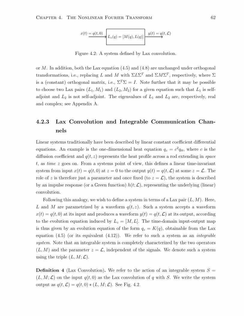
Chapter 4. The Nonlinear Fourier Transform 62
Lz(q) = [M(q), L(q)]x(t) = q(t, 0) y(t) = q(t,L)
Figure 4.2: A system defined by Lax convolution.
or M . In addition, both the Lax equation (4.5) and (4.8) are unchanged under orthogonal
transformations, i.e., replacing L and M with ΣLΣT and ΣMΣT , respectively, where Σ
is a (constant) orthogonal matrix, i.e., ΣTΣ = I. Note further that it may be possible
to choose two Lax pairs (L1,M1) and (L2,M2) for a given equation such that L1 is self-
adjoint and L2 is not self-adjoint. The eigenvalues of L1 and L2 are, respectively, real
and complex; see Appendix A.
4.2.3 Lax Convolution and Integrable Communication Chan-
nels
Linear systems traditionally have been described by linear constant coefficient differential
equations. An example is the one-dimensional heat equation qz = c2qtt, where c is the
diffusion coefficient and q(t, z) represents the heat profile across a rod extending in space
t, as time z goes on. From a systems point of view, this defines a linear time-invariant
system from input x(t) = q(t, 0) at z = 0 to the output y(t) = q(t,L) at some z = L. The
role of z is therefore just a parameter and once fixed (to z = L), the system is described
by an impulse response (or a Green function) h(t;L), representing the underlying (linear)
convolution.
Following this analogy, we wish to define a system in terms of a Lax pair (L,M). Here,
L and M are parametrized by a waveform q(t, z). Such a system accepts a waveform
x(t) = q(t, 0) at its input and produces a waveform y(t) = q(t,L) at its output, according
to the evolution equation induced by Lz = [M,L]. The time-domain input-output map
is thus given by an evolution equation of the form qz = K(q), obtainable from the Lax
equation (4.5) (or its equivalent (4.12)). We refer to such a system as an integrable
system. Note that an integrable system is completely characterized by the two operators
(L,M) and the parameter z = L, independent of the signals. We denote such a system
using the triple (L,M ;L).
Definition 4 (Lax Convolution). We refer to the action of an integrable system S =
(L,M ;L) on the input q(t, 0) as the Lax convolution of q with S. We write the system
output as q(t,L) = q(t, 0) ∗ (L,M ;L). See Fig. 4.2.

Chapter 4. The Nonlinear Fourier Transform 63
Definition 5 (Integrable communication channels). A waveform communication chan-
nel C : x(t) × v(t, z) → y(t) with inputs x(t) ∈ L1(R) and space-time noise v(t, z) ∈L2(R,R+), and output y(t) ∈ L1(R), is said to be integrable if the noise-free channel is
an integrable system.
Note that noise can be introduced into an integrable system in a variety of ways.
In what follows, we assume that the signal-to-noise ratio is not too small, so that the
stochastic system may justifiably be considered as a perturbation of the deterministic
system. Furthermore, in this thesis we limit ourselves to integrable channels with additive
noise, i.e.,
qz = K(q) + v(t, z), q(t, 0) = x(t), q(t,L) = y(t),
where v(t, z) is distributed band-limited noise. Note that this model is not in general
equivalent to one in which noise is added (in lumped fashion) at the channel output.
Here, the noise is distributed in space, and so interacts with the signal (in a potentially
very complicated manner) according to the given evolution equation.
In this thesis, we develop a scheme for communication over integrable channels. By
various choices of Lax pair (L,M), one can construct a variety of interesting channel
models, mostly nonlinear, which go beyond the linear channel models typically studied
in data communications. Interestingly, some linear channels can also be analyzed us-
ing this nonlinear spectral approach advocated here [49]. The central application (and
motivation) for this work is fiber-optic communication, in which the channel model is
given by the nonlinear Schrodinger equation (3.1), and for which a Lax pair was given
in Example 10. In what follows, we first discuss the deterministic (noise-free) case and
later treat noise as a perturbation of the deterministic system.
4.3 Nonlinear Fourier Transform
In this section, we assume that a function q(t, ·) ∈ L1(R) is given, and we define its
nonlinear Fourier transform with respect to a given Lax operator L. As the notation
q(t, ·) implies, in this and the next section, the variable z can take on any value in the
range [0,L] and is irrelevant in the forward and inverse transforms. We shall therefore
omit the index z in what follows.
As previously noted, for concreteness we carry through the development of the NFT

Chapter 4. The Nonlinear Fourier Transform 64
for the case of the NLS equation (3.3), for which the P - and M -equations are given by
vt = P (λ, q)v =
(−jλ q(t, z)
−q∗(t, z) jλ
)v, (4.18)
vz = M(λ, q)v
=
(2jλ2 − j|q(t, z)|2 −2λq(t, z)− jqt(t, z)
2λq∗(t, z)− jq∗t (t, z) −2jλ2 + j|q(t, z)|2
)v, (4.19)
respectively. Here the P -equation is the Zakharov-Shabat system.
The nonlinear Fourier transform (and its inverse) are defined solely in terms of the
temporal P -equation (4.18). The spatial M -equation (4.19) is used in a brief, and critical,
propagation step, but plays no role in the definition of the nonlinear Fourier transform.
If for a given λ ∈ C, the operator L−λI, here equivalent to DI−P representing (4.18),
is not invertible, we say that λ belongs to the spectrum of L and v(t, λ) represents its
associated eigenfunction. In finite-dimensional Hilbert spaces of matrices the spectrum is
a discrete finite set, called eigenvalues. This may no longer be true in infinite-dimensional
spaces of operators, where the eigenvalues (if they exist) may only be one part of the
spectrum. See Appendix A.
The nonlinear Fourier transform of a signal x(t) with respect to an operator L in a
Lax pair is defined via the spectral analysis of the L operator, which we consider next.
4.3.1 Canonical Eigenvectors and Spectral Coefficients
We wish to study solutions of (4.18), in which vectors v(t) are considered as elements of
the vector space H. We begin by equipping the vector space H with a symplectic bilinear
form H×H 7→ C, which, for any fixed value of t ∈ R, is defined as
〈v(t), w(t)〉s = v1(t)w2(t)− v2(t)w1(t). (4.20)
Let us also define the adjoint of any vector v in H as
v(t) =
(v∗2(t)
−v∗1(t)
).
The following properties hold true for all v and w in H:
• ˜v = −v;
• 〈v, v〉s = 0;
• 〈v, w〉s = −〈w, v〉s;

Chapter 4. The Nonlinear Fourier Transform 65
• 〈v, v〉s = −〈v, v〉s = |v1|2 + |v2|2;
• ddt〈v, w〉s = 〈vt, w〉s + 〈v, wt〉s;
• for every 2× 2 matrix A, 〈Av,w〉s + 〈v, Aw〉s = tr(A)〈v, w〉s.There are generally infinitely many solutions v of (4.18) for a given λ ∈ C, parametrized
by the set of all possible boundary conditions. These solutions form a subspace Eλ of
continuously differentiable 2× 1 vector functions (an eigenspace).
Lemma 7. For all vectors v(t) and w(t) in Eλ,
1. v ∈ Eλ∗, i.e., vt = P (λ∗, q)v;
2. 〈v(t), w(t)〉s is a constant, independent of t;
3. If 〈v(t), w(t)〉s 6= 0, then v and w are linearly independent and form a basis for
Eλ;
4. dim(Eλ) = 2.
Proof : Property 1) follows directly from (4.18). To see 2), note that ddt〈v, w〉s =
〈vt, w〉s + 〈v, wt〉s = 〈Pv, w〉s + 〈v, Pw〉s = tr(P )〈v, w〉s = 0. To see 3), fix t and let
u(t) ∈ Eλ, then u(t) = a(t)v(t) + b(t)w(t) for some a(t) and b(t). Taking the symplectic
inner product of both sides with w and v, we get a(t) = 〈u,w〉s/〈v, w〉s and b(t) =
〈u, v〉s/〈w, v〉s. From Property 2, 〈u,w〉s, 〈v, w〉s, 〈u, v〉s, and 〈w, v〉s are all independent
of t. It follows that a and b are also independent of t. Finally, 4) follows from 3).
An important conclusion of Lemma 7 is that any two linearly independent solutions
u and w of (4.18) provide a basis for the solution space. To choose two such solutions, we
examine the behavior of the equation at large values of |t|. If we assume that q(t, ·)→ 0
as |t| → ∞, then, as |t| → ∞ (4.18) is reduced to
vt →(−jλ 0
0 jλ
)v, for large |t|,
which has a general solution
v(t, λ)→[αe−jλt, βejλt
]T, α, β ∈ C.
Two possible boundary conditions, bounded in the upper half complex plane (=(λ) >
0), are
v1(t, λ)→(
0
1
)ejλt, t→ +∞ (4.21)
v2(t, λ)→(
1
0
)e−jλt, t→ −∞. (4.22)

Chapter 4. The Nonlinear Fourier Transform 66
t = ∞
v1(t, λ∗) →(01
)ejλ
∗t
t = −∞
v2(t, λ∗) →(−10
)e−jλ∗t
v2(t, λ∗)
v2(t, λ) →(10
)e−jλt v1(t, λ) →
(01
)ejλt
v1(t, λ∗)
Figure 4.3: Boundary conditions for the canonical eigenvectors.
We solve (4.18) for a given λ under the boundary conditions (4.21)-(4.22), and denote
the resulting solutions for all t ∈ R as v1(t, λ) and v2(t, λ). We can also solve (4.18) for
λ∗ under the adjoint boundary conditions
v1(t, λ∗)→(
0
1
)ejλ∗t, t→ +∞, (4.23)
v2(t, λ∗)→(−1
0
)e−jλ
∗t, t→ −∞,
giving rise to two solutions v1(t, λ∗) and v2(t, λ∗). From Lemma 7 we have that v1(t, λ∗)
and v2(t, λ∗) are elements of Eλ. These four eigenfunctions v1(t, λ), v2(t, λ), v1(t, λ∗), and
v2(t, λ∗), all of them elements of Eλ, are called canonical eigenvectors. Fig. 4.3 illustrates
the canonical eigenvectors at their boundaries.
Lemma 8. Canonical eigenvectors satisfy:
1. 〈v1(t, λ∗), v1(t, λ〉s = 〈v2(t, λ∗), v2(t, λ)〉s = 1;
2. v1(t, λ), v1(t, λ∗) and v2(t, λ), v2(t, λ∗) are independent sets in Eλ.
Proof : 1) Since 〈v1, v1〉s is independent of t, using (4.21) and (4.23), 〈v1(t, λ∗), v1(t, λ)〉s =
〈v1(+∞, λ∗), v1(+∞, λ)〉s = 1. 2) Follows from 1) and Lemma 7.
Choosing v1(t, λ∗) and v1(t, λ) as a basis of Eλ, one can project v2(t, λ), v2(t, λ∗) ∈ Eλon this basis to obtain
v2(t, λ) = a(λ)v1(t, λ∗) + b(λ)v1(t, λ), (4.24)
v2(t, λ∗) = b∗(λ∗)v1(t, λ∗)− a∗(λ∗)v1(t, λ), (4.25)
where a(λ) = 〈v2, v1〉s and b(λ) = 〈v1, v2〉s. A crucial property, following from Lemma 7,
is that a(λ) and b(λ) are time-independent. The time-independent complex scalars a(λ)
and b(λ) are called the nonlinear Fourier coefficients [9, 10].

Chapter 4. The Nonlinear Fourier Transform 67
Since the nonlinear Fourier coefficients are time independent, to facilitate computing
them, for simplicity we can send t to, e.g., +∞ where v1(+∞, λ) and v1(+∞, λ∗) are
known. The other two canonical eigenvectors v2 and v2 are then propagated from their
boundary values v2(−∞, λ) and v2(−∞, λ∗) at t = −∞ according to v2t = P (λ, q)v2 and
v2t = P (λ∗, q)v2 to obtain v2(∞, λ) and v2(∞, λ∗). At this stage, we have available all
four canonical eigenvectors at one time, namely,
v2(+∞, λ), v2(+∞, λ), v1(+∞, λ), v1(+∞, λ)
.
We can now project v2(+∞, λ) and v2(+∞, λ) onto the basis v1(+∞, λ) and v1(+∞, λ)
according to (4.24)-(4.25) to obtain
[v2(+∞, λ), v2(+∞, λ)
]=[v1(+∞, λ), v1(+∞, λ)
]S, (4.26)
where
S =
(a(λ) b∗(λ∗)
b(λ) −a∗(λ∗)
). (4.27)
The matrix S is called the scattering matrix and contains the nonlinear Fourier coef-
ficients [9, 10]. It is a function of q(t, ·) and says how the solution to (4.18) is scattered
from t = −∞ to t = +∞. More precisely, the field v2(−∞, λ) = [1, 0]T e−jλt is applied
at t = −∞, where q is absent. This field evolves forward in time according to (4.18),
interacts with the signal (which can be viewed as an “obstacle”) at finite values of t,
and subsequently propagates towards t = +∞, where again q is absent. The field at
t = +∞ is measured and gives information about the “obstacle” as seen from a distance.
Although not obvious from the development so far, we shall see in Section 4.6 that the
information measured at t = +∞, captured by a(λ) and b(λ), is complete, in the sense
that from this information we can retrieve q(t, ·) entirely. In view of this interpreta-
tion, the nonlinear Fourier transform was historically referred to as the inverse scattering
transform.
4.3.2 The Nonlinear Fourier Transform
The projection equations (4.24) and (4.25) that give a(λ) and b(λ) are well-defined if
λ ∈ R. From Lemma 7, Property 1), we observe that the eigenspace is symmetric in
λ, i.e., if λ is an eigenvalue then so is λ∗. Thus it is sufficient to consider the upper
half complex plane C+ = λ|=(λ) > 0. In this region, the boundary conditions on the

Chapter 4. The Nonlinear Fourier Transform 68
basis vectors v1 and v1 at t = ∞ decay and blow up, respectively. As a result, (4.24) is
consistent in C+ only if a(λ) = 0. Eigenvalues in C+ are therefore identified as the zeros
of the complex function a(λ) and they form the discrete (point) spectrum of the signal.
We will see in the next section that the discrete spectrum corresponds to soliton pulses.
Lemma 9. If q(t) ∈ L1(R), a(λ) is an analytic function of λ on C+.
Proof : From Lemma 10 in Section 4.6, if q(t) ∈ L1(R) the scaled canonical eigenvec-
tors v1(t, λ)e−jλt and v2(t, λ)ejλt are analytic functions of λ in C+. Since
a(λ) = 〈v2, v1〉s = 〈v2ejλt, v1e−jλt〉s,
is a combination of two analytic functions in C+, it is analytic in the same region. (Note,
however, that b(λ), which is a combination of functions analytic in disjoint regions in C,
may not be analytic in either of those regions.)
A consequence of Lemma 9 is that the zeros of a(λ) in C+ are isolated points [50]. It
follows that the Zakharov-Shabat operator for the NLS equation has two types of spectra.
The discrete (or point) spectrum, which occurs in C+, is characterized by those λj ∈ C+
satisfying
a(λj) = 0, j = 1, 2, . . . , N.
The discrete spectrum corresponds to solitons, and in this case (4.24) reduces to
v2(t, λj) = b(λj)v1(t, λj).
The continuous spectrum, which in general includes the whole real line =(λ) = 0, cor-
responds to the non-solitonic (or radiation) component of the signal. The continuous
spectrum is the component of the NFT which corresponds to the ordinary Fourier trans-
form, whereas the discrete spectrum has no analogue in linear systems theory. The reader
is referred to Appendix A for a number of examples illustrating various notions of the
spectrum associated with bounded linear operators; Example 18 is particularly relevant
to the discussion here.
To distinguish between the discrete and continuous spectra, we find it convenient to
refer to discrete spectral values of λ using the symbol λj (with a subscript). Continuous
spectral values are denoted as λ (without a subscript). In general, λj ∈ C+, whereas
λ ∈ R.
For the purpose of developing the inverse transform, we find it sufficient to work with

Chapter 4. The Nonlinear Fourier Transform 69
the ratios
q(λ) =b(λ)
a(λ), q(λj) =
b(λj)
a′(λj),
where a′(λj) denotes the derivative da(λ)dλ
∣∣∣λ=λj
.
We can now formally define the nonlinear Fourier transform of a signal with respect
to a given Lax operator L as follows.
Definition 6 (Nonlinear Fourier transform [9, 37]). Let q(t) be a sufficiently smooth
function in L1(R). The nonlinear Fourier transform of q(t) with respect to a given Lax
operator L consists of the continuous and discrete spectral functions q(λ) : R 7→ C and
q(λj) : C+ 7→ C where
q(λ) =b(λ)
a(λ), q(λj) =
b(λj)
a′(λj), j = 1, 2, . . . , N,
in which λj are the zeros of a(λ). Here, the spectral coefficients a(λ) and b(λ) are given
by
a(λ) = = limt→∞
v21ejλt, (4.28)
b(λ) = = limt→∞
v22e−jλt, (4.29)
where v2(t, λ) is a solution of (4.18) under the boundary condition (4.22).
To obtain the continuous spectral function q(λ), λ ∈ R, it is not necessary to obtain
a(λ) and b(λ) separately. For convenience, one can instead write an explicit differential
equation
dy(t, λ)
dt+ q(t)e2jλty2(t, λ) + q∗(t)e−2jλt = 0,
y(−∞, λ) = 0, (4.30)
and obtain q(λ) = limt→∞ y(t, λ).
Analogously, one can solve the second-order differential equation
d2z(t, λ)
dt2−(
2jλ+qtq
)dz(t, λ)
dt+ |q|2z(t, λ) = 0,
z(−∞, λ) = 1,dz(−∞, λ)
dt= 0, (4.31)
and obtain a(λ) = limt→∞
z(t, λ). The discrete spectrum is obtained as the zeros of a(λ).
Remark 10. The NFT is generally operator specific and thus is defined with respect to an
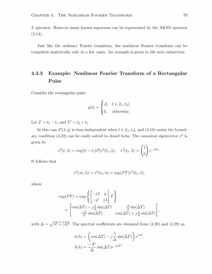
Chapter 4. The Nonlinear Fourier Transform 70
L operator. However many known equations can be represented by the AKNS operator
(4.14).
Just like the ordinary Fourier transform, the nonlinear Fourier transform can be
computed analytically only in a few cases. An example is given in the next subsection.
4.3.3 Example: Nonlinear Fourier Transform of a Rectangular
Pulse
Consider the rectangular pulse
q(t) =
A, t ∈ [t1, t2];
0, otherwise.
Let T = t2 − t1 and T ′ = t2 + t1.
In this case P (λ, q) is time-independent when t ∈ [t1, t2], and (4.18) under the bound-
ary condition (4.22) can be easily solved in closed form. The canonical eigenvector v2 is
given by
v2(t, λ) = exp[(t− t1)P ]v2(t1, λ), v2(t1, λ) =
(1
0
)e−jλt1 .
It follows that
v2(∞, λ) = v2(t2, λ) = exp(PT )v2(t1, λ),
where
exp(PT ) = exp
[−jλ q
−q∗ jλ
]T
=
[cos(∆T )− j λ
∆sin(∆T ) A
∆sin(∆T )
−A∗∆
sin(∆T ) cos(∆T ) + j λ∆
sin(∆T )
],
with ∆ =√λ2 + |A|2. The spectral coefficients are obtained from (4.28) and (4.29) as
a(λ) =
(cos(∆T )− j λ
∆sin(∆T )
)ejλT ,
b(λ) =−A∗
∆sin(∆T )e−jλT
′.

Chapter 4. The Nonlinear Fourier Transform 71
0
0.5
1
1.5
2
2.5
-30 -20 -10 0 10 20 30
|q(λ)|
λ
-10123456
-1 -0.5 0 0.5 1
ℑ(λ)
ℜ(λ)
0
0.5
1
1.5
2
2.5
-40 -30 -20 -10 0 10 20 30 40
|q(λ)|
λ
-10123456
-1 -0.5 0 0.5 1
ℑ(λ)
ℜ(λ)
(a) (b)
0
0.5
1
1.5
2
2.5
-40 -30 -20 -10 0 10 20 30 40
|q(λ)|
λ
-10123456
-1 -0.5 0 0.5 1
ℑ(λ)
ℜ(λ)
(c)
Figure 4.4: Discrete and continuous spectra of a square wave signal with T = 1, and (a)A = 1, (b) A = 2, (c) A = 6.
The zeros of a(λ) in C+, which satisfy
j tan(T√|A|2 + λ2) =
√1 +|A|2λ2
,
give rise to the discrete spectrum. The continuous spectrum is given by
q(λ) =A∗
jλe−2jλt2
(1− ∆
jλcot(∆T )
)−1
.
Note that as A→ 0, ∆→ λ, and one can see that in the limit of AT 1 there is no
discrete spectrum. Furthermore, the continuous spectrum tends to
q(λ) = −A∗Te−jλT ′sinc(2Tf), λ = 2πf,
which is just the ordinary Fourier transform of the q(t).
Fig. 4.4 shows the two spectra for T = 1 and various values of A. For small A, there is
no discrete spectrum and the continuous spectrum is essentially just the ordinary Fourier

Chapter 4. The Nonlinear Fourier Transform 72
transform of q(t). As A is increased, the continuous spectrum deviates from the ordinary
Fourier transform and one or more discrete mass points appear on the jω axis.
4.3.4 Elementary Properties of the Nonlinear Fourier Trans-
form
Let q(t)↔ (q(λ), q(λk)) be a nonlinear Fourier transform pair. The following properties
are proved in Appendix C.1.
1. (The ordinary Fourier transform as limit of the nonlinear Fourier transform): If
||q||L1 1, there is no discrete spectrum and q(λ) → Q(λ), where Q(λ) is the
ordinary (linear) Fourier transform of −q∗(t)
Q(λ) = −∞
−∞
q∗(t)e−2jλtdt.
2. (Weak nonlinearity): If |a| 1, then aq(λ) ≈ aq(λ) and aq(λk) ≈ aq(λk). In
general, however, aq(λ) 6= aq(λ) and aq(λk) 6= aq(λk).
3. (Constant phase change): ejφq(t)(λ) = ejφq(t)(λ) and ejφq(t)(λk) = ejφq(t)(λk).
4. (Time dilation): q( ta) = |a|q(aλ) and q( t
a) = |a|q(aλk);
5. (Time shift): q(t− t0)↔ e−2jλt0 (q(λ, )q(λk));
6. (Frequency shift): q(t)e−2jωt ↔ (q(λ− ω), q(λk − ω));
7. (Lax convolution): If q2(t) = q1(t) ∗ (L,M ;L), then q2(λ) = H(λ,L)q1(λ) and
q2(λk) = H(λ,L)q1(λk). For the NLS equation, the channel filter is H(λ,L) =
exp(−4jλ2L).
8. (Parseval identity):∞
−∞‖q(t)‖2 dt = E + E, where
E =1
π
∞
−∞
log(1 + |q(λ)|2
)dλ, E = 4
N∑
j=1
= (λj) .
The quantities E and E represent the energy contained in the continuous and
discrete spectra, respectively.
In addition, we have the following properties related to the nonlinear Fourier trans-
form
1. (Causality and layer-peeling property): Let q1(t) and q2(t) be two signals with
non-overlapping support, e.g., signals in a pulse train. Without loss of generality,
assume that q1(t) is supported on t ≤ t0, and that q2(t) is supported on t > t0. If

Chapter 4. The Nonlinear Fourier Transform 73
(a1, b1) and (a2, b2) are, respectively, the nonlinear Fourier coefficients of q1(t) and
q2(t), then the nonlinear Fourier coefficients of q1(t) + q2(t) are given by
(a(λ), b(λ)) = (a1(λ), b1(λ)) (a2(λ), b2(λ))∆=(a1(λ)a2(λ)− b1(λ)b∗2(λ∗), a1(λ)b2(λ) + b1(λ)a∗2(λ∗)
).
That is to say, if we slice the signal in time in consecutive portions according to
a mesh −∞ < · · · < t−1 < t0 < t1 < · · · < ∞, the nonlinear Fourier coefficients
satisfy the Markov property
ak(λ), bk(λ); q(t), tk < t < tk+1 → (ak+1(λ), bk+1(λ)) ,
where (ak(λ), bk(λ)) are the spectral coefficients calculated from q(t) in −∞ < t <
tk.
2. (Purely imaginary eigenvalues) If ||q||L1 <π2, then there is no discrete spectrum.
If q(t) is real, nonnegative, piecewise smooth, and single-lobe (non-decreasing for
t < t0 and non-increasing for t > t0), then there are precisely N = b12
+||q(t)||L1
π−εc
eigenvalues, all purely imaginary and simple [51].
4.4 Evolution of the Nonlinear Fourier Transform
Derivation of the evolution of the nonlinear Fourier transform of a signal propagating
based on the NLS equation proceeds straightforwardly. As q(t, z) propagates, the eigen-
values of L are preserved and the eigenvectors of L propagate based on (4.19). Assuming
that q(t, z) and its time-derivative vanish at t = ±∞ for all z ≤ L during the propagation,
then as t→∞ (4.19) is reduced to
vz(t, z)→(
2jλ2 0
0 −2jλ2
)v(t, z). (4.32)
Thus the boundary conditions (4.21) and (4.22) are transformed to
v1(t, λ)→(
0
1
)ejλte−2jλ2z, t→ +∞,
v2(t, λ)→(
1
0
)e−jλte2jλ2z, t→ −∞.

Chapter 4. The Nonlinear Fourier Transform 74
These transformed boundary conditions are not consistent with the boundary conditions
(4.21) and (4.22) used to define the canonical eigenvectors, due to the additional factors
e±2jλ2z. As a result, the evolution of the canonical eigenvectors from z = 0, according
to vz = Mv, does not lead to the canonical eigenvectors at z = L. However, by proper
scaling, one can obtain the canonical eigenvectors at any z.
For instance, focusing on v2(t, λ; z), and changing variables to u2(t, λ; z) = v2(t, λ; z)e−2jλ2z,
we obtain u2t = Pu2 with boundary condition (4.22) for all z. Consequently, u2(t, λ; z) is
a canonical eigenvector for all z. By transforming (4.32), the evolution equation for u is
asymptotically (at t = +∞) given by
u2z(∞, λ; z) =
(0 0
0 −4jλ2z
)u2(∞, λ; z),
which gives
u21(∞, λ; z) = u2
1(∞, λ; 0)
u22(∞, λ; z) = u2
2(∞, λ; 0)e−4jλ2z
Using expressions (4.28) and (4.29) we obtain
a(λ, z) = limt→∞
u21(t, λ; z)ejλt = lim
t→∞u2
1(t, λ; 0)ejλt = a(λ, 0)
b(λ, z) = limt→∞
u22(t, λ; z)e−jλt = lim
t→∞u2
2(t, λ; 0)e−4jλ2ze−jλt
= b(λ, 0)e−4jλ2z.
In turn, the nonlinear Fourier transform propagates according to
q(t, z)(λ) = e−4jλ2z q(t, 0)(λ),
q(t, z)(λj) = e−4jλ2jz q(t, 0)(λj),
λj(z) = λj(0), j = 1, 2, . . . , N. (4.33)
Note that, since a(λ, z) is preserved under the evolution (i.e., is independent of z), the
number of the discrete eigenvalues—which are zeros of a(λ)—are also preserved.
In summary, we see that the operation of the Lax convolution in the nonlinear Fourier
domain is described by a simple multiplicative (diagonal) operator, much in the same
way that the ordinary Fourier transform maps y(t) = x(t) ∗ h(t) to Y (ω) = X(ω) ·H(ω).
The channel filter in (4.33) is exp(−4jλ2z).

Chapter 4. The Nonlinear Fourier Transform 75
4.5 An Approach to Communication over Integrable
Channels
Since the nonlinear Fourier transform of a signal is essentially preserved under Lax con-
volution, one can immediately conceive of a nonlinear analogue of orthogonal frequency
division multiplexing (OFDM) for communication over integrable channels. We refer to
this scheme as nonlinear frequency division multiplexing (NFDM). In this scheme, the
input output channel model is given by
Y (λ) = H(λ)X(λ) + Z(λ)
Y (λj) = H(λj)X(λj) + Z(λj),
where X(λ) = q(λ, 0) and X(λj) = q(λ, 0) are spectra at the input of the channel,
Y (λ) = q(λ, z) and Y (λj) = q(λ, z) are spectra at the output of the channel, Z(λ) and
Z(λj) are effective noises in the spectral domain, and the channel filter is
H(λ) = e−4jλ2z.
A bandlimited Gaussian noise in time domain generally maps to non-Gaussian noise
processes in the spectral domain.
The proposed scheme consists of two steps.
• The inverse nonlinear Fourier transform at the transmitter (INFT). At the trans-
mitter, information is encoded in the nonlinear spectra of the signal according to a
suitable constellation on(X(λ), X(λj)
). The time domain signal is generated by
taking the inverse nonlinear Fourier transform,
q(t) = INFT(X(λ), X(λ)
),
and is sent over the channel. (The INFT is described formally in the next section.)
• The forward nonlinear Fourier transform at the receiver (NFT). At the receiver,
the (forward) nonlinear Fourier transform of the signal,
(Y (λ), Y (λ)
)= NFT(q(t, z))
is taken and the resulting spectra are compared against the transmitted spectra
according to some metric d(X(λ), X(λ); Y (λ), Y (λ)
).
As q(t, 0) propagates in the time domain based on the complicated nonlinear equa-
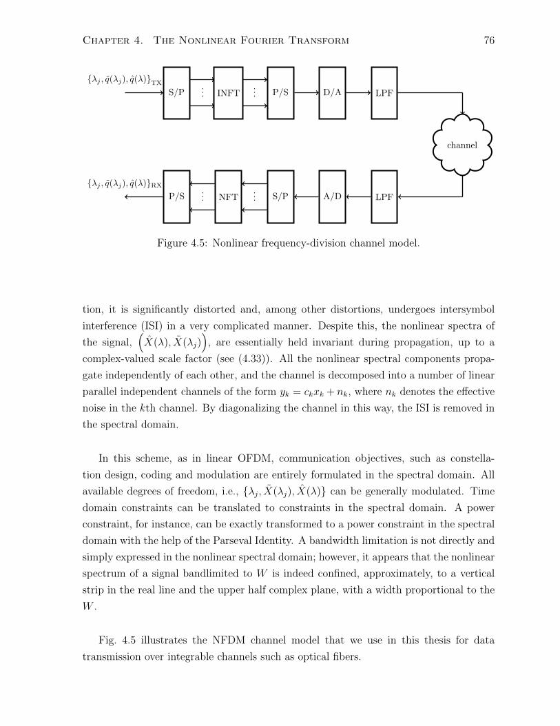
Chapter 4. The Nonlinear Fourier Transform 76
λj , q(λj), q(λ)TX
S/P INFT P/S D/A LPF
P/S NFT S/P A/D LPF
λj , q(λj), q(λ)RX
......
......
channel
Figure 4.5: Nonlinear frequency-division channel model.
tion, it is significantly distorted and, among other distortions, undergoes intersymbol
interference (ISI) in a very complicated manner. Despite this, the nonlinear spectra of
the signal,(X(λ), X(λj)
), are essentially held invariant during propagation, up to a
complex-valued scale factor (see (4.33)). All the nonlinear spectral components propa-
gate independently of each other, and the channel is decomposed into a number of linear
parallel independent channels of the form yk = ckxk + nk, where nk denotes the effective
noise in the kth channel. By diagonalizing the channel in this way, the ISI is removed in
the spectral domain.
In this scheme, as in linear OFDM, communication objectives, such as constella-
tion design, coding and modulation are entirely formulated in the spectral domain. All
available degrees of freedom, i.e., λj, X(λj), X(λ) can be generally modulated. Time
domain constraints can be translated to constraints in the spectral domain. A power
constraint, for instance, can be exactly transformed to a power constraint in the spectral
domain with the help of the Parseval Identity. A bandwidth limitation is not directly and
simply expressed in the nonlinear spectral domain; however, it appears that the nonlinear
spectrum of a signal bandlimited to W is indeed confined, approximately, to a vertical
strip in the real line and the upper half complex plane, with a width proportional to the
W .
Fig. 4.5 illustrates the NFDM channel model that we use in this thesis for data
transmission over integrable channels such as optical fibers.
Chapter 4. The Nonlinear Fourier Transform 77
4.6 Inverse Nonlinear Fourier transform
In this section, we describe the inverse nonlinear Fourier transform, which is a method
for recovering the signal q(t, ·) from its nonlinear Fourier transform (q(λ), q(λj)). This is
the opposite of what was done in the Section 4.3, and it gives further important insight
into the mechanism of the NFT. As in Section 4.3, the value of z is irrelevant here and
the index z is thus suppressed.
4.6.1 Riemann-Hilbert Factorization
In the 1950s, before the publication of Gardner [42], a method for retrieving the poten-
tial q(t) in the linear Schrodinger equation from the knowledge of the scattering matrix
S was already known in quantum mechanics. It was later realized that this method is
an instance of a Riemann-Hilbert problem in complex analysis [10, 37]. Alternatively,
the same task can be accomplished using the Gelfand-Levitan method [10], a different
approach developed earlier in the context of inverse problems for Sturm-Liouville differ-
ential equations. Although either of these methods can be used for solving the inverse
problem, in this thesis we will use the Riemann-Hilbert method.
To begin, canonical eigenvectors can be found in two ways. On the one hand, they
are related to q(t) through the Zakharov-Shabat system (4.18). One can solve (4.18) to
explicitly express the canonical eigenvectors as a series involving q(t). On the other hand,
canonical eigenvectors are related to the nonlinear Fourier transform via the projection
equations (4.24)-(4.25). The latter are two equations for four unknowns and in general
cannot be solved. However, the unique properties of the canonical eigenvectors, which
are analytic in disjoint regions of the complex plane, will allow us to find them in terms
of the nonlinear Fourier transform. Note that this second derivation does not explicitly
depend on q(t); however, by equating the canonical eigenvectors obtained from these two
derivations, we can relate the signal q(t) to its nonlinear Fourier transform (q(λ), q(λj)).
We find it helpful to briefly introduce the tool that we employ in this section, namely
the Riemann-Hilbert factorization problem in complex analysis.
Definition 7 (Riemann-Hilbert factorization). The Riemann-Hilbert factorization prob-
lem consists of finding two complex functions f−(z) and f+(z), respectively, analytic in-
side and outside of a closed contour C in the complex plane, such that on C they satisfy
the boundary condition f+(z) = g(z)f−(z) for some given g(z).
It g(z) satisfies a Holder condition, it is possible to find both f+(z) and f−(z) ev-
erywhere in the complex plane from the given boundary condition. In Appendix B, we
Chapter 4. The Nonlinear Fourier Transform 78
provide a brief overview of this problem and its solution. See [52] for more discussion.
4.6.2 The Inverse Transform
The inverse transform maps the two spectral functions (q(λ), q(λj)) to the signal q(t).
As noted, we need to express the canonical eigenvectors in terms of the nonlin-
ear Fourier transform. Below we will find it more convenient to work with canonical
eigenvectors subject to fixed boundary conditions. Scaling the canonical eigenvectors as
V 2 = v2ejλt, V 2(t, λ∗) = v2(t, λ∗)e−jλt, V 1 = v1e−jλt and V 1(t, λ∗) = v1(t, λ∗)ejλt, the
projection equations (4.24) and (4.25) are transformed to
V 2(t, λ) = a(λ)V 1(t, λ∗) + b(λ)e2jλtV 1(t, λ), (4.34)
V 2(t, λ∗) = −a∗(λ∗)V 1(t, λ) + b∗(λ∗)e−2jλtV 1(t, λ∗). (4.35)
Lemma 10. If q ∈ L1(R), then V 1(t, λ) and V 2(t, λ) are analytic functions of λ in the
upper half complex plane C+ = z ∈ C : =(z) > 0 while V 1(t, λ∗) and V 2(t, λ∗) are
analytic functions of λ in the lower half complex plane C− = z ∈ C : =(z) < 0.
Proof. See Appendix C.2.
Rearranging (4.34)-(4.35) gives
(V 1(t, λ) V 2(t, λ)
)
=(V 1(t, λ∗) V 2(t, λ∗)
)( b∗(λ∗)a∗(λ∗)e
−2jλt 1a∗(λ∗)
−1a∗(λ∗) − b(λ)
a∗(λ∗)e−2jλt
). (4.36)
Since(V 2 V 1
)and
(V 2(t, λ∗) V 1(t, λ∗)
)are analytic, respectively, in the upper and
lower half-planes, (4.36) defines a matrix Riemann-Hilbert problem.
Solution of the Riemann-Hilbert factorization problem (4.36) is given in Appendix C.4.
Omitting the details, the following linear system of equations, known as the Riemann-
Chapter 4. The Nonlinear Fourier Transform 79
Hilbert system, is obtained:
V 1(t, λ∗) =
(1
0
)+
N∑
i=1
q(λi)e2jλitV 1(t, λi)
λ− λi
+1
2πj
∞
−∞
q(ζ)e2jζtV 1(t, ζ)
ζ − (λ− jε) dζ,
V 1(t, λ) =
(0
1
)−
N∑
i=1
q∗(λ∗i )e−2jλ∗i tV 1(t, λ∗i )
λ− λ∗i
+1
2πj
∞
−∞
q∗(ζ∗)e−2jζtV 1(t, ζ∗)
ζ − (λ+ jε)dζ,
V 1(t, λ∗m) =
(1
0
)+
N∑
i=1
q(λi)e2jλitV 1(t, λi)
λ∗m − λi
+1
2πj
∞
−∞
q(ζ)e2jζtV 1(t, ζ)
ζ − λ∗mdζ, m = 1, . . . , N,
V 1(t, λm) =
(0
1
)−
N∑
i=1
q∗(λ∗i )e−2jλ∗i tV 1(t, λ∗i )
λm − λ∗i
+1
2πj
∞
−∞
q∗(ζ∗)e−2jζtV 1(t, ζ∗)
ζ − λmdζ,
m = 1, . . . , N. (4.37)
This is a system of 2N + 2 linear equations for 2N + 2 discrete and continuous canonical
eigenvectors V 1(t, λm)Nm=1, V 1(t, λm)Nm=1, and V 1(t, λ) and V 1(t, λ) as a function of
the Fourier transform (q(λ), q(λj)).
Next, the canonical eigenvectors are related to the signal q(t). By inspecting the
Zakharov-Shabat system (4.18), it is shown in Appendix C.3 that for |λ| 1
V 1(t, λ) =
12jλq(t)
1 + 12jλ
∞
−∞|q(t)|2dt
+O(λ−2). (4.38)
It now becomes easy to recover the signal q(t) from the nonlinear Fourier transform
(q(λ), q(λj)). Eigenvector V 1 is related to q via (4.38) for |λ| 1, and is related to the
nonlinear Fourier transform via the second equation in (4.37). Approximating 1/(λ− ζ)
Chapter 4. The Nonlinear Fourier Transform 80
and 1/(λ − λi) by −1/λ + O(λ−2) in the second equation of (4.37) for |λ| 1 and
comparing V 11 with V 1
1 in (4.38), we obtain
q∗(t) = 2jN∑
i=1
q(λi)e2jλitV 1
2 (t, λi)
− 1
π
ˆ ∞−∞
q(λ)e2jλtV 12 (t, λ)dλ. (4.39)
This represents q(t) as a function of the nonlinear Fourier transform.
In summary, given (q(λ), q(λj)), we first solve the Riemann-Hilbert system to find the
eigenvector V 1. For this purpose, one can discretize the system (4.37) and solve a linear
system of equations of the form
Ax = b,
for appropriate A and b. This is done for each fixed ti to determine the samples of
V l(ti, λ) at that time. Then, V 1, q and q are substituted in (4.39) to obtain the signal
q(t).
Note that this inverse transform is taken only once at the transmitter to synthesize
the desired pulse shapes. It is only the forward transform which needs to be taken in
real time at the receiver.
The mathematical tools developed in this chapter are used in the subsequent chap-
ters to present further details pertaining the application of the suggested scheme in data
transmission over integrable channels. In the next chapter, numerical methods are pre-
sented to compute NFT. An important special case occurs when the continuous spectrum
is zero. This corresponds to N -soliton signals, where the inverse NFT can be carried out
in several ways. N -solitons are discussed in Chapter 6.
4.7 Summary
The nonlinear Fourier transform of a signal with respect to an operator L in a Lax
pair consists of continuous and discrete spectral functions x(λ) and x(λj), obtainable by
solving the eigenproblem for the L operator. The NFT maps a Lax convolution to a
multiplication operator in the spectral domain. Using the nonlinear Fourier transform,
we propose a transmission scheme for integrable channels, termed nonlinear frequency-
division multiplexing, in which the information in encoded in the nonlinear spectrum of
the signal. The scheme is an extension of traditional OFDM to any channel generated by

Chapter 4. The Nonlinear Fourier Transform 81
a Lax pair. An example is the optical fiber channel, in which signals propagate according
to the nonlinear Schrodinger equation. The class of integrable channels, though nonlinear
and often complicated, are somehow “linear in disguise,” and thus admit the proposed
nonlinear frequency-division multiplexing transmission scheme.

Chapter 5
Numerical Methods For Computing
the NFT
The purpose of computing is insight,
not numbers.
Richard Hamming
The nonlinear Fourier transform of a signal q(t) is a pair of functions: the continuous
spectrum q(λ), λ ∈ R, and the discrete spectrum q(λj), =λj > 0, j = 1, . . . ,N. The
NFT arises in the study of integrable waveform channels as defined in Chapter 4. In
such channels, signals propagate (in a potentially complicated manner) according to a
given integrable evolution equation, whereas the nonlinear Fourier transform of the signal
propagates according to a (simple) multiplication operator.
In Chapter 4, we proposed nonlinear frequency-division multiplexing (NFDM), a
scheme that uses the nonlinear Fourier transform for data communication over inte-
grable channels. NFDM extends traditional orthogonal frequency division multiplexing
(OFDM) to channels generatable by a Lax pair. An example is the optical fiber channel,
where signal propagation is modeled by the (integrable) nonlinear Schrodinger (NLS)
equation. In general, the channel input-output relations in the NFT domain are (see
Chapter 4)
Y (λ) = H(λ)X(λ) + Z(λ),
Y (λj) = H(λj)X(λj) + Z(λj),
where X(λ) and X(λj) are continuous and discrete spectra at the input of the channel,
Y (λ) and Y (λj) are spectra at the output of the channel, and Z(λ) and Z(λj) represent
82
Chapter 5. Numerical Methods For Computing the NFT 83
noise. The channel filter H(λ) for the NLS equation is given by H(λ) = exp(−4jλ2z).
NFDM is able to deal directly with nonlinearity and dispersion, without the need
for additional compensation at the transmitter or receiver. In this scheme, informa-
tion is encoded in the nonlinear spectrum at the channel input, and the corresponding
time-domain signal is transmitted. At the receiver, the NFT of the received signal is
computed, and the resulting spectra Y (λ) and Y (λj) are subsequently used to recover
the transmitted information.
Similar to the ordinary Fourier transform, while the NFT can be computed analyti-
cally in a few cases, in general, numerical methods are required. Such methods must be
robust, reliable and fast enough to be implemented in real time at the receiver. In this
chapter, we suggest and evaluate the performance of a number of numerical algorithms for
computing the forward NFT of a given signal. Using these algorithms, we then perform
extensive numerical simulations to understand the behavior of the nonlinear spectrum
for various pulse shapes and parameters commonly used in data communications.
We are aware of no published work presenting the NFT of various signals numeri-
cally, for different pulse shapes and parameters. Such work is necessary to clarify the
structure of the nonlinear spectrum and help in its understanding. In part, this has been
due to the fact that the NFT has largely remained a theoretical artifice, and practical
implementation of the NFT as an applied tool has not yet been pursued in engineering.
We review the relevant literature in Section 5.1 and suggest new schemes for the
numerical evaluation of the NFT. Although these methods are general and work for the
AKNS system [48], for the purpose of illustration, we specialize the AKNS system to
the Zakharov-Shabat system. All these methods are put to test in cases where analyt-
ical formulae exist and are compared with one another in Section 5.5. Only some of
these methods will be chosen for the subsequent numerical simulations; these are the
layer-peeling method, Ablowitz-Ladik integrable discretization, and the spectral matrix
eigenvalue scheme. These methods are used in the next sections to numerically compute
the nonlinear Fourier transform of a variety of practical pulse shapes encountered in data
communications.
5.1 The Nonlinear Fourier Transform
Details of the nonlinear Fourier transform can be found in Chapter 4. Here we briefly re-
call a few essential ingredients required in the numerical computation of the forward
transform. As noted earlier, we illustrate numerical methods in the context of the
Zakharov-Shabat system, which is a Lax operator for the nonlinear Schrodinger equation.
Chapter 5. Numerical Methods For Computing the NFT 84
For later use, we recall that the slowly-varying complex envelope q(t, z) of a narrow-
band small-amplitude signal propagating in a dispersive weakly-nonlinear medium, such
as an optical fiber, satisfies the cubic nonlinear Schrodinger equation. By proper scaling,
the equation can be normalized to the following dimensionless form in 1 + 1 dimensions:
jqz = qtt + 2|q|2q. (5.1)
Here t denotes retarded time, and z is distance.
The NFT for an integrable evolution equation starts by finding a Lax pair of operators
L and M such that the evolution equation arises as the compatibility condition Lz =
[M,L] = ML− LM . For the NLS equation, we may take operator L as
L = j
(∂∂t
−q(t, z)−q∗(t, z) ∂
∂t
). (5.2)
(The corresponding M operator can be found in Chapter 4.)
The NFT is defined via the spectral analysis of the L operator (5.2). The spectrum
of L is found by solving the eigenproblem Lv = λv, where λ is an eigenvalue of L and
v is its associated eigenvector. It can be shown that the operator L in (5.2) has the
isospectral flow property, i.e., its spectrum is invariant even as q evolves according to the
NLS equation.
The eigenproblem Lv = λv can be simplified to
vt =
(−jλ q(t)
−q∗(t) jλ
)v. (5.3)
Note that the z-dependence of q is suppressed in (5.3) (and throughout this chapter),
as this variable comes into play only in the propagation of the signal, not in the definition
and computation of the NFT.
Assumption 1. Throughout this thesis we assume that (a) q ∈ L1(R), and (b) q(t) is
supported in the finite interval [T1, T2].
The set of eigenvectors v associated with eigenvalue λ in (5.3) is a two-dimensional
subspace Eλ of the continuously differentiable functions. We define the adjoint of a vector
v = [v1(t), v2(t)]T as v = [v∗2(t),−v∗1(t)]T . If v(t, λ∗) is an element of Eλ∗ , then v(t, λ∗) is
an element of Eλ. It can be shown that any pair of eigenvectors v(t, λ) and v(t, λ∗) form
a basis for Eλ (see Section 4.3.1). Using Assumption 1(b), we can select an eigenvector

Chapter 5. Numerical Methods For Computing the NFT 85
v1(t, λ) to be a solution of (5.3) with the boundary condition
v1(T2, λ) =
(0
1
)ejλT2 .
The basis eigenvectors v1 and v1 are called canonical eigenvectors.
Having identified a basis for the subspace Eλ, we can project any other eigenvector
v2 on this basis according to
v2(t, λ) = a(λ)v1(t, λ) + b(λ)v1(t, λ). (5.4)
Following Assumption 1(b), a particular choice for v2 is made by solving the system
vt =
(−jλ q(t)
−q∗(t) jλ
)v, v(T1, λ) =
(1
0
)e−jλT1 , (5.5)
in which we dropped the superscript 2 in v2 for convenience. By solving (5.5) in the
interval [T1, T2] for a given λ and obtaining v(T2, λ), the nonlinear Fourier coefficients
a(λ) and b(λ) can be obtained by considering (5.4) at t = T2. The resulting coefficients
obtained in this manner are
a(λ) = v1(T2)ejλT2 ,
b(λ) = v2(T2)e−jλT2 . (5.6)
The NFT of a signal q(t) consists of a continuous spectral function defined on the
real axis λ ∈ R
q(λ) =b(λ)
a(λ), λ ∈ R,
and a discrete spectral function defined on the upper half complex plane C+ = λ :
=(λ) > 0
q(λj) =b(λj)
da(λ)/dλ|λ=λj
, j = 1, · · · ,N,
where λj are eigenvalues and correspond to the (isolated) zeros of a(λ) in C+, i.e.,
a(λj) = 0.
From the discussions made, in order to compute the nonlinear spectrum of q(t), the
system of differential equations (5.5) needs to be solved in the interval [T1, T2]. Except

Chapter 5. Numerical Methods For Computing the NFT 86
for special cases, (5.5) needs to be solved numerically.
Numerical methods for the calculation of the forward nonlinear Fourier transform are
divided into two classes in this chapter:
1. Methods which estimate the continuous spectrum by directly integrating the
Zakharov-Shabat system; see Section 5.2.
2. Methods which find the (discrete) eigenvalues. Two approaches are suggested in
this thesis for this purpose. Similar to the continuous spectrum estimation, we
can integrate the Zakharov-Shabat system numerically and obtain a(λ). To find
zeros of a(λ), the scheme is often supplemented with a search method to locate
eigenvalues in the upper half complex plane. One can also discretize and rewrite
the Zakharov-Shabat system in the interval [T1, T2] as a (large) matrix eigenvalue
problem; see Section 5.3.
We begin by discussing methods which estimate the continuous spectrum.
5.2 Numerical Methods for Computing the Contin-
uous Spectrum
In this section, we assume that λ ∈ R is given and provide algorithms for calculating
the nonlinear Fourier coefficients a(λ) and b(λ). The continuous spectral function is then
easily computed as the ratio q(λ) = b(λ)/a(λ). This process can be repeated to compute
the spectral amplitudes for any desired finite set of continuous frequencies λ.
5.2.1 Forward and Central Discretizations
The most obvious method to attempt to solve (5.5) is the first-order Euler method or
one of its variations [53].
Recall that the signal q(t) is supported in the finite time interval [T1, T2], and partition
this interval uniformly according to the mesh T1 < T1 + ε < · · · < T1 +Nε = T2 with size
N , i.e., with ε = (T2 − T1)/N . Let q[k]∆= q(kε) and let
P [k]∆=
(−jλ q[k]
−q∗[k] jλ
). (5.7)
Integrating both sides of (5.5) from kε to (k+ 1)ε and assuming that the right hand side
Chapter 5. Numerical Methods For Computing the NFT 87
is constant over this interval, we get
v[k + 1] = v[k] + εP [k]v[k], k = 0, . . . , N,
v[0] =
(1
0
)e−jλT1 . (5.8)
Equation (5.8) is iterated from k = 0 to k = N to find v[N ]. The resulting vector is
subsequently substituted in (5.6) to obtain a(λ) and b(λ).
We have implemented the Euler method for the calculation of the nonlinear Fourier
transform of a number of pulse shapes. Unfortunately, the one-step Euler method does
not produce satisfactory results for affordable small step sizes ε.
One can improve upon the basic Euler method by considering the central difference
iteration [53],
v[k + 1] = v[k − 1] + 2εP [k]v[k].
This makes the discretization second-order, i.e., the error v(T1 + kε) − v[k] is of order
O(ε2). Here an additional initial condition is required too, which can be obtained, e.g.,
by performing one step of the regular forward difference (5.8).
5.2.2 Fourth-order Runge-Kutta Method
One can also employ higher-order integration schemes such as the Runge-Kutta methods.
Improved results are obtained using the fourth-order Runge-Kutta method [54–56]. How-
ever it takes significant time to estimate the spectrum using such higher order numerical
methods in real-time. Since the method, with its typical parameters, is quite slow and
does not outperform some of the schemes suggested in the following sections, we do not
elaborate on this method here; see [53] for details. However, for comparison purposes we
will include this scheme in our numerical simulations given in Section 5.5.
5.2.3 Layer-peeling Method
In Section 4.3.3 of Chapter 4, we have calculated the nonlinear spectra of a rectangular
pulse. One can approximate q(t) as a piece-wise constant signal and use the layer-peeling
property of the nonlinear Fourier transform to estimate the spectrum of any given signal.
Let a[k] and b[k] be the nonlinear Fourier coefficients of q(t) in the interval [T1, kε), and
x[k] and y[k] coefficients in the small (rectangular) region [kε, kε + ε). The iterations of

Chapter 5. Numerical Methods For Computing the NFT 88
the layer-peeling method read
(a[k + 1], b[k + 1]) = (a[k], b[k]) (x[k], y[k]), (5.9)
(a[0], b[0]) = (1, 0),
where the operation is defined as in [57]
a[k + 1] = a[k]x[k]− b[k]y[k],
b[k + 1] = a[k]y[k] + b[k]x[k],
in which
x[k] =
(cos(Dε)− j λ
Dsin(Dε)
)ejλ(t[k]−t[k−1]),
y[k] =−q∗kD
sin(Dε)e−jλ(t[k]+t[k−1]),
and x[k](λ) = x∗[k](λ∗), y[k](λ) = y∗[k](λ∗), D =√λ2 + |q[k]|2. The desired coefficients
are obtained as a := a[N ] and b := b[N ]. Note that the exponential factors in x[k]
and y[k] enter in a telescopic manner. As a result, for the numerical implementation,
it is faster to drop these factors and just scale the resulting a[N ] and b[N ] coefficients
by exp(jλ(T2 − T1)) and exp(−jλ(T2 + T1)), respectively. This, however, reduces the
accuracy as it involves the product of large and small numbers.
We are motivated by [37] in which the layer-peeling identity (5.9) is mentioned as a
property of the nonlinear Fourier transform. An equivalent presentation of this method
is given in [56,58,59] as well.
Note further that a different numerical method, but with the same name (layer-
peeling), exists in geophysics and fiber Bragg design [60]; however this method is not
related to the problem considered here.
We shall see in Section 5.5 that the layer-peeling method gives remarkably accurate
results in estimating the nonlinear Fourier transform.
5.2.4 Crank-Nicolson Method
In the Crank-Nicolson method, the derivative of the evolution parameter is approximated
by a finite-difference approximation, e.g., forward discretization, and other functions are

Chapter 5. Numerical Methods For Computing the NFT 89
discretized by taking their average over the end points of the discretization interval:
v[k + 1]− v[k]
ε=
1
2(P [k]v[k] + P [k + 1]v[k + 1]) ,
where P [k] is defined in (5.7). This implicit iteration can be made explicit
v[k + 1] = (I − ε
2P [k + 1])−1(I +
ε
2P [k])v[k],
k = 0, . . . , N
with initial condition (5.8). As we will see, this simple scheme too gives good results in
estimating the nonlinear spectrum.
5.2.5 The Ablowitz-Ladik Discretization
Ablowitz-Ladik discretization is an integrable discretization of the NLS equation in time
domain [61, 62]. In this section, we suggest using the Lax pairs of the Ablowitz-Ladik
discretization of the NLS equation for solving the Zakharov-Shabat eigenproblem in the
spectral domain [63].
Discretization sometimes breaks symmetries, making the discrete version of an in-
tegrable equation no longer integrable. A consequence of symmetry-breaking is that
quantities that are conserved in the continuous model may no longer be invariant in the
discretized equation. A completely integrable Hamiltonian system with an infinite num-
ber of conserved quantities might have a discretized version with no, or few, conserved
quantities. The discrete equation therefore does not quite mimic the essential features of
the original equation if the step size is not small enough.
However, for some integrable equations, discretizations exist which are themselves
completely integrable Hamiltonian systems, i.e., they possess an infinite number of con-
served quantities and are linearizable by a Lax pair, and therefore are solvable by the
nonlinear Fourier transform. Such developments exist for the NLS and Korteweg-de Vries
(KdV) equations.
For the NLS equation, the integrable discrete version was introduced by Ablowitz
and Ladik [61]. To illustrate the general idea, let us replace 1 ± jλε for small ε with
e±jλε in the forward discretization method (5.8) (the opposite of what is usually done in
practice). Let z = e−jλε represent the discrete eigenvalue, Q[k] = q[k]ε, and
R[k] =
(z Q[k]
−Q∗[k] z−1
). (5.10)

Chapter 5. Numerical Methods For Computing the NFT 90
The Ablowitz-Ladik iteration is
v[k + 1] = R[k]v[k], v[0] =
(1
0
)e−jλT1 . (5.11)
Under this z transformation, the upper half complex plane in λ domain is mapped to the
exterior of the unit circle in the z domain. The continuous spectrum therefore lies on the
unit circle |z| = 1, while the discrete spectrum lies outside of the unit circle |z| > 1.
One can rewrite the R-equation (5.10) in the eigenvalue form Lv[k] = zv[k], with the
following L operator
L =
(Z −Q[k]
−Q∗[k − 1] α[k − 1]Z−1
), (5.12)
where α[k] = 1 + |Q[k]|2, and Z is the shift operator, i.e., Z−1x[k] = x[k− 1], k ∈ Z. To
the first order in ε, α[k] ≈ 1 and (5.12) can be simplified to
L =
(Z −Q[k]
−Q∗[k] Z−1
). (5.13)
Given the L operator (5.13), one can consider the M operator of the continuous NLS
equation and modify its elements such that the compatibility equation Lz = [M,L]
represents a discretized version of the NLS equation. It is not hard to verify that after
doing so we are led to an M operator resulting in the following discrete integrable NLS
equation
jdq[k]
dz=q[k + 1]− 2q[k] + q[k − 1]
ε2
+ |q[k]|2(q[k + 1] + q[k − 1]). (5.14)
Here the space derivative remains intact and the signal q[k] is discretized in time, in
such a way that the nonlinearity is somehow averaged among three time samples. In the
continuum limit ε → 0, (5.14) approaches the continuous NLS equation and its merits
lie in the fact that it is integrable for any ε, not just in the limit ε → 0. For example,
soliton pulses can be observed in this model for any ε. The equation has its own infinite
number constants of motion, approaching integrals of motion in the continuum limit.
The operator M which leads to (5.14), and the details of the nonlinear Fourier transform
for (5.14) can be found in [9, 61].
We conclude that the Ablowitz-Ladik discretization can be used not only as a means

Chapter 5. Numerical Methods For Computing the NFT 91
to discretize the NLS equation in the time domain, but also as a means to solve the
continuous-time Zakharov-Shabat system in the spectral domain. This is a non-finite-
difference discretization, capable of dealing with oscillations exp(±jλt) in the Zakharov-
Shabat system, which greatly enhances the accuracy of the one-step finite-difference
methods.
Following the Tao and Thiele’s approach [37] and [54], we can also normalize the R[K]
matrix
v[k + 1] =1√
1 + |Q[k]|2
(z Q[k]
−Q[k]∗ z−1
)v[k]. (5.15)
The scale factor does not change the spectrum significantly, since it is canceled out in
the ratios q = b/a and q = b/a′, and also its effects are second order in ε. However,
numerically, normalization may help in reducing the numerical error. In subsequent
sections, we refer to (5.11) as the Ablowitz-Ladik method (AL1) and to (5.15) as the
modified Ablowitz-Ladik method (AL2).
5.3 Methods for Calculating the Discrete Spectrum
In order to compute the discrete spectrum, the zeros of a(λ) in the upper half complex
plane must be found. One way to visualize this is to assume a two-dimensional mesh in
C+ and determine a at all mesh points. Discrete eigenvalues are then easily identified by
looking at the graph of |a(λ)|; in many cases they correspond to deep and narrow “wells”
corresponding to the zeros of the magnitude of a.
As noted earlier, two types of methods are suggested to calculate the point spectrum.
1. One can use the integration-based algorithms mentioned in Section 5.2 which
calculate nonlinear Fourier coefficients, and search for eigenvalues using a root
finding method, such as the Newton-Raphson method. Such methods require
good initial points and one needs to be careful about convergence [53].
2. It is also possible to rewrite the spectral problem for an operator as a (large)
matrix eigenvalue problem. The point spectrum of the operator can be found in
this way too.
5.3.1 Search Methods
To calculate the discrete spectral amplitude q = b/a′, we require da/dλ as well. As we
will show, information about the derivative of a can be updated recursively along with
Chapter 5. Numerical Methods For Computing the NFT 92
the information about a, without resorting to approximate numerical differentiation.
Recall that the nonlinear Fourier coefficient a(λ) is given by (5.6)
a(λ) = v1[N ]ejλt[N ].
Taking the derivative with respect to λ, we obtain
da(λ)
dλ= ((v1[N ])′ + jT2v1[N ]) ejλt[N ].
We can update the derivative information dv/dλ along with v. In methods of Section 5.2,
the transformation of eigenvectors from t[k] to t[k + 1] can be generally represented as
v[k + 1] = A[k]v[k],
for some suitable one-step update matrix Ak (which varies from method to method).
Differentiating with respect to λ and augmenting v with v′ = dv/dλ, we get the iterations
v[k + 1] = A[k]v[k], (5.16)
v′[k + 1] = A′[k]v[k] + A[k]v′[k], (5.17)
with initial conditions
v[0] =
(1
0
)e−jλt[0], v′[0] =
(−jt[0]
0
)e−jλt[0].
The derivative matrix A′ depends on the method used.
For the forward discretization scheme:
A′ = M1 =
(−j 0
0 j
)ε.
For the Crank-Nicolson scheme:
A′ =1
2(I +M2)−1 (I + (I +M2)−1 (I −M2)
)M1,
where
M2 =
(12jλ −1
2q[k]
12q∗[k] −1
2jλ
)ε.

Chapter 5. Numerical Methods For Computing the NFT 93
For the Ablowitz-Ladik method:
A′ =
(−jz 0
0 jz−1
)ε.
The desired coefficients are obtained at k = N as follows
a(λ) = v1[N ]ejλt[N ],
b(λ) = v2[N ]e−jλt[N ],
a′(λ) = (v′1[N ] + jt[N ]v1[N ]) ejλt[N ].
Similarly, the layer-peeling iteration can be augmented to update a′(λ) as well:
a[k + 1] = a[k]x[k]− b[k]y[k],
b[k + 1] = a[k]y[k] + b[k]x[k],
a′[k + 1] = a′[k]x[k] + a[k]x′[k]− (b′[k]y[k] + b[k]y′[k]),
b′[k + 1] = a′[k]y[k] + a[k]y′[k] + b′[k]x[k] + b[k]x′[k],
a[0] = 1, b[0] = a′[0] = b′[0] = 0, (5.18)
where
x[k] = cos(Dε)− j λD
sin(Dε),
y[k] =−q∗kD
sin(Dε),
x′[k] = −jλ2ε
D2cos(Dε)−
(j + λε
D− jλ2
D3
)sin(Dε),
y′[k] = −q∗kλ
D3(Dε cos(Dε)− sin(Dε)) .
The expressions for x′[k] and y′[k] are similar, with j replaced with −j and q[k] replaced
with −q∗[k].
With the derivative information being available, the Newton-Raphson method is a
good scheme to search for the location of the (discrete) eigenvalues. The iteration for the
complex-valued Newton-Raphson scheme is
λk+1 = λk − αka(λk)
a′(λk), (5.19)
where αk is some step size modifier; usually αk = 1. The iteration stops if λk is almost

Chapter 5. Numerical Methods For Computing the NFT 94
stationary, i.e., if |α aa′ | < δ for a small δ. In practice, the quadratic convergence of the
scheme is often very fast and occurs in just a few iterations.
In data communications, since noise is usually small, the points in the transmitted
constellation can (repeatedly) serve as the initial conditions for (5.19). In this case,
convergence is usually achieved in a couple of iterations. For an unknown signal, random
initial conditions are chosen. In either case, one or more sequence of Newton iterations
have to be performed for any single eigenvalue.
To make sure that all of the eigenvalues are found, we can check the trace formula
for n = 1, 2, 3. The trace formula is a time frequency identity relating the hierarchy of
infinitely many conserved quantities to the spectral components.
In general, the trace formula represents a time domain conserved quantity as the sum
of discrete and continuous spectral terms:
E(k) = E(k)disc + E
(k)cont,
where
E(k)disc =
4
k
N∑
i=1
=(λki),
E(k)cont =
1
π
∞
−∞
λk−1 log(1 + |q(λ)|2
)dλ,
and where E(k) are time domain conserved quantities (functionals of the signal). The
first few conserved quantities are energy
E(1) =
∞
−∞
|q(t, z)|2dt,
momentum
E(2) =1
2j
∞
−∞
q(t)dq(t)
dtdt,
and Hamiltonian
E(3) =1
(2j)2
∞
−∞
(|q(t)|4 −
∣∣∣∣dq(t)
dt
∣∣∣∣2)
dt.

Chapter 5. Numerical Methods For Computing the NFT 95
For n = 1, the trace formula is a kind of Parseval’s identity (Plancherel’s theorem),
representing the total energy of the signal in time as the sum of the energy of the discrete
and continuous spectral functions. When satisfied, the Parseval’s identity ensures that
all of the signal energy has been accounted for.
We first calculate the continuous spectrum and its “energy terms” for a sufficiently
fine mesh on the real λ axis. The energy difference Eerror =∣∣∣∣∣∣E(k) − E(k)
cont
∣∣∣∣∣∣ gives an
estimate on the number of missing eigenvalues. When a new eigenvalue λ is found, this
error is updated as Eerror :=∣∣∣∣∣∣E(k) − E(k)
cont − 4k=λk
∣∣∣∣∣∣. The process is repeated until Eerror
is less than a small prescribed tolerance value.
To summarize, given the signal q(t), its nonlinear Fourier transform can be computed
based on Algorithm 1.
5.3.2 Discrete Spectrum as a Matrix Eigenvalue Problem
The methods mentioned in Section 5.3.1 find the discrete spectrum by searching for
eigenvalues in the upper half complex plane. Sometimes it is desirable to have all eigen-
values at once, which can be done by solving a matrix eigenvalue problem [55,63]. These
schemes obviously estimate only (discrete) eigenvalues and do not give information on
the rest of the spectrum. Since the matrix eigenvalue problem can be solved quickly
for small-sized problems, it might take less computational effort to compute the discrete
spectrum in this way. In addition, one does not already need the continuous spectrum
to estimate the size of the discrete spectrum. On the other hand, for large matrices that
arise when a large number of signal samples are used, the matrix eigenproblem (which
is usually not Hermitian) is slow and it may be better to find the discrete spectrum
using the search-based methods. The matrix-based methods also have the disadvantages
that they can generate a large number of spurious eigenvalues, and one may not be able
to restrict the algorithm for finding eigenvalues of a matrix to a certain region of the
complex plane.
Below we rewrite some of the methods mentioned in the Section 5.2 as a regular
matrix eigenvalue problem, for the computation of the discrete spectrum.

Chapter 5. Numerical Methods For Computing the NFT 96
Algorithm 1 Numerical Nonlinear Spectrum Estimation
Sample the signal at a sufficiently small step size ε.Fix a sufficiently fine mesh M on the real λ axis.for each λ ∈M do
Iterate (5.16) from k = 0 to k = N to obtain v[N ].Compute the continuous spectral amplitude
ρ(λ) =v2[N ]
v1[N ]e−2jλt[N ].
end forInitialize the error e = ||E − Econt||.while |e| > ε1 do
Choose λ0 ∈ D randomly, where D is a prescribed region in C+.Set i = 0;repeat
Iterate (5.16)-(5.17) from k = 0 to k = N to obtain v[N ] and v′[N ], and performa Newton-Raphson update
λi+1 = λi −∆λ, ∆λ = αiv1[N ]
v′1[N ] + jt[N ]v1[N ]
if If λi+1 /∈ D thenchoose λ0 ∈ D randomly.Set i := −1.
end ifSet i := i+ 1.
until |∆λ| < ε2 and i > 0λi is an eigenvalue and the associated spectral amplitude is
q(λi) =v2[N ]
v′1[N ] + jt[N ]v1[N ]e−2jλit[N ].
Update e := ||E − Econt − Edisc||, where Edisc = [4=λi, 2=λ2i ,
43=λ3
i ].end while

Chapter 5. Numerical Methods For Computing the NFT 97
Central-difference Eigenproblem
The matrix eigenvalue problem can be formulated in the time domain or the frequency
domain [55]. Consider the Zakharov-Shabat system in the form Lv = λv
j
(∂∂t
−q−q∗ − ∂
∂t
)v = λv. (5.20)
In the time domain, one can replace the time derivative ∂/∂t by the central finite-
difference matrix
D =1
2ε
0 1 0 · · · −1
−1 0 1 · · · 0
· · ·0 0 −1 0 1
1 0 0 −1 0
,
and expand (5.20) as
j
(D −diag(q[k])
−diag(q∗[k]) −D
)v[k] = λv[k]. (5.21)
The point spectrum is contained in the eigenvalues of the matrix in the left hand side of
(5.21).
Eigenvalues of a real symmetric or Hermitian matrix can be found relatively efficiently,
owing to the existence of a complete orthonormal basis and the stability of the eigenvalues.
In this case, a sequence of unitary similarity transformations Ak+1 = PAkPT can be
designed, using, for instance, the QR factorization, the Householder transformation, etc.,
to obtain the eigenvalues rather efficiently [64].
Unfortunately, most of the useful statements about computations using Hermitian
matrices cannot usually be generalized to non-Hermitian matrices. As a result, the
eigenvalues of a non-Hermitian matrix (corresponding to a non-self-adjoint operator) are
markedly difficult to calculate [64,65]. Running a general-purpose eigenvalue calculation
routine on (5.21) is probably not the most efficient way to get eigenvalues. Next we
make suggestions to simplify the non-Hermitian eigenproblem (5.21) by exploiting its
structure.
The diagonal matrix in the lower left corner of (5.21) can be made zero by apply-
ing elementary row operations and using the entries of the D matrix. Since elementary
row operations, as in Gauss-Jordan elimination, generally change the eigenvalues, the

Chapter 5. Numerical Methods For Computing the NFT 98
corresponding column operations are also applied to induce a similarity transformation.
In this way, an upper-Hessenberg matrix is obtained in O(N) operations, as compared
to a sequence of Householder transformations with O(N3) operations and O(N2) mem-
ory registers. The eigenvalues of the resulting complex upper-Hessenberg matrix can
subsequently be found using QR iterations.
Ablowitz-Ladik Eigenproblem
We can also rewrite the Ablowitz-Ladik discretization as a matrix eigenvalue problem.
Using the L operator (5.13), we obtain
v1[k + 1]−Q[k]v2[k] = zv1[k], (5.22)
−Q∗[k − 1]v1[k] + α[k − 1]v2[k − 1] = zv2[k], (5.23)
which consequently takes the form
(U1 −diag(Q[k])
−diag(Q∗[k − 1]) UT2
)v = zv,
in which
U1 =
0 1 0 · · · 0
0 0 1 · · · 0
· · ·0 0 0 0 1
1 0 0 0 0
,
U2 =
0 α[1] 0 · · · 0
0 0 α[2] · · · 0
· · ·0 0 0 0 α[N − 1]
α[N ] 0 0 0 0
,
and diag(Q[k]) = diag (Q[0], · · · , Q[N ]), diag(Q∗[k−1]) = diag (Q∗[N ], Q∗[0] · · · , Q∗[N − 1]).
Note that all shifting operations are cyclic, so that all vector indices k remain in the in-
terval 0 ≤ k ≤ N .
It is not very different to consider the more simplified L operator (5.12) instead
of (5.13). This corresponds to the above discretization with U2 := U1 and −Q∗[k − 1]
replaced with −Q∗[k]. Similarly, one can rewrite the normalized Ablowitz-Ladik iteration

Chapter 5. Numerical Methods For Computing the NFT 99
as a matrix eigenvalue problem. This corresponds to (5.23) where instead of having α[k−1], v1[k + 1] is multiplied by α[k] in the first equation, i.e., U1 and U2 are interchanged.
Spectral Method
In the frequency domain, one can approximate derivatives with the help of the Fourier
transform. Let us assume that
v(t) =
M2∑
k=−M2
(αk
βk
)ej2kπtT , q(t) =
M2∑
k=−M2
γkej2kπtT ,
where T = T2 − T1. Then the Zakharov-Shabat system is
−αk2πk
T− j
M2∑
m=−M2
γk−mβm = λαk,
−jM2∑
m=−M2
γ∗−k+mαm + βk2πk
T= λβk.
Thus we obtain
(Ω Γ
−ΓH −Ω
)(α
β
)= jλ
(α
β
),
where α = [α−M2, . . . , αM
2]T , β = [β−M
2, . . . , βM
2]T , Ω = −2π
Tdiag(−M
2, . . . , M
2) and
Γ = −j
γ0 γ−1 · · · γ−M2
0 0 · · · 0
γ1 γ0 γ−1 · · · γ−M2
0 · · · 0. . . . . . . . .
γM2γM
2−1 · · · γ−M
2+1 γ−M
2
0 γM2γM
2−1 · · · γ−M
2+1
. . . . . . . . .
0 · · · 0 γM2γM
2−1 · · · γ0 γ−1
0 0 · · · 0 γM2γM
2−1 · · · γ0
.
The point spectrum is thus found by looking at the eigenvalues of the matrix
A =
(Ω Γ
−ΓH −Ω
).

Chapter 5. Numerical Methods For Computing the NFT 100
5.4 Running Time, Convergence and Stability of the
Numerical Methods
The numerical methods discussed in this chapter are first-order matrix iterations and
therefore the running time of all of them is O(N) multiplications and additions per
eigenvalue. This corresponds to a complexity of O(N2) operations for the calculation of
the continuous spectrum on a mesh with N eigenvalues. The exact number of operations
depends on the details of the implementation and the memory requirement of the method.
All iterative methods thus take about the same time asymptotically, albeit with different
coefficients.
An important observation is that, while the Fast Fourier Transform (FFT) takes
O(N log2N) operations to calculate the spectral amplitudes of a vector with length N
at N equispaced frequencies, the complexity of the methods described in this chapter to
compute the continuous spectrum are O(N2). Similarly, it takes O(NN) operations to
calculate the discrete spectrum. In other words, so far we do not exploit the potentially
repetitive operations in our computations.
It is evident from (5.6) that as T2 → ∞, v1[k] should grow as ∼ exp(−jλT2) so
that a(λ) is a finite complex number. The canonical eigenvector v[k;T1, T2] thus has an
unbounded component as T2 → ∞ (i.e., ||v[k]|| → ∞). One can, however, normalize v1
and v2 according to
u1 = v1ejλt
u2 = v2e−jλt,
and transform (5.5) to
ut =
(0 q(t)e2jλt
−q∗(t)e−2jλt 0
)u, u(T1, λ) =
(1
0
). (5.24)
The desired coefficients are simply a(λ) = u1(T2) and b(λ) = u2(T2). Consequently, if
one is interested in obtaining eigenvectors v[k] in addition to the coefficients a(λ) and
b(λ), the discretization of the normalized system (5.24) has better stability properties:
(a[k + 1], b[k + 1]) =
(1 Q[k]z−2k
−Q∗[k]z2k 1
)(a[k], b[k])
(a[0], b[0]) = (1, 0) . (5.25)

Chapter 5. Numerical Methods For Computing the NFT 101
The nonlinear Fourier coefficients are obtained as a := a[N ] and b := b[N ]. The discrete
nonlinear Fourier transform mentioned in [37] is thus the forward discretization of the
normalized Zakharov-Shabat system (5.24).
We are interested in the convergence of v[k] (or a(λ) and b(λ)) as a function of N for
fixed values of T1 and T2. That is to say, we require that the error e = ||v(kε)− v[k]|| → 0
as N → ∞ (for fixed T1 and T2). The (global) error in all methods described in this
chapter is at least O(ε), and therefore all these methods are convergent.
Some of these methods are, however, not stable. This is essentially because the
Zakharov-Shabat system in its original form has unbounded solutions, i.e., ||v(t)|| → ∞as t → ∞. Errors can potentially be amplified by the unstable system poles. One
should be cautious about the normalized system (5.24) as well. For example, forward
discretization of the normalized system (5.25) gives a first-order iteration x[k + 1] =
A[k]x[k]. The eigenvalues of the matrix A[k] in this method are
s1,2 = 1± jε|q[k]|.
It follows that the forward discretization of (5.24) gives rise to eigenvalues outside of
the unit disk, |s| > 1. As a result, first-order discretization of (5.24) are also unstable.
In cases where |s| > 1, we can consider normalizing the iterations by dividing A[k] by√detA[k] (in the case of (5.25), dividing the right-hand side by
√1 + |Q[k]|2). The
resulting iteration has eigenvalues inside the unit disk. For ε 1 the effect is only
second-order in ε, however it helps in managing the numerical error if larger values of ε
are chosen.
An issue pertinent to numerical methods is chaos. Chaos and numerical instability of
finite-difference discretizations has been observed in [66] for the sine-Gordon equation,
which is also integrable and shares a number of basic properties with the NLS equation.
In [67], the authors conclude that the standard discretizations of the cubic nonlinear
Schrodinger equation may lead to spurious numerical behavior. This instability is deeply
related to the homoclinic orbits of the NLS equation, i.e., it occurs if the initial signal
q(t, z = 0) is chosen to be close to the homoclinic orbit of the equation. It disappears
only if the step size is made sufficiently small, which can be smaller than what is desired
in practice.
It is shown in [67] that the Ablowitz-Ladik discretization of the NLS equation (in time)
has the desirable property that chaos and numerical instability, which are sometimes
present in finite-difference discretizations of the NLS equation, do not appear at all.
Though these results are for the original time-domain equations, the issue can occur in

Chapter 5. Numerical Methods For Computing the NFT 102
the spectral eigenvalue problem (5.5) as well, if the signal q[k] is close to a certain family
of functions (related to sinωt and cosωt). Therefore, among discretizations studied, the
Ablowitz-Ladik discretization of the Zakharov-Shabat system is immune to chaos and its
resulting numerical instability. This is particularly important in the presence of amplifier
noise, where chaos can be more problematic.
5.5 Testing and Comparing the Numerical Methods
In this section, we test and compare the ability of the suggested numerical schemes to
estimate the nonlinear Fourier transform (with respect to the Zakharov-Shabat system)
of various signals. Numerical results are compared against analytical formulae, in a few
cases where such expressions exist. Our aim is to compare the speed and the precision of
these schemes for various pulse shapes in order to determine which ones are best suited
for subsequent simulation studies.
To derive the analytical formulae, recall that the continuous spectral function can be
written as q(λ) = limt→∞
y(t, λ), in which y(t, λ) satisfies [57]
dy(t, λ)
dt+ q(t)e2jλty2(t, λ) + q∗(t)e−2jλt = 0,
y(−∞, λ) = 0. (5.26)
Similarly, one can solve the second-order differential equation
d2z(t, λ)
dt2−(
2jλ+qtq
)dz(t, λ)
dt+ |q|2z(t, λ) = 0,
z(−∞, λ) = 1,dz(−∞, λ)
dt= 0, (5.27)
and obtain a(λ) = limt→∞
z(t, λ). The zeros of a(λ) form the discrete spectrum.
In the following, the discrete spectrum is found and compared using the following
matrix-based schemes:
1. central difference method;
2. spectral method;
3. Ablowitz-Ladik (AL) discretization (AL1);
4. AL discretization with normalization (AL2).
In the matrix-based schemes, the entire point spectrum is found at once by solving a
matrix eigenvalue problem.
The complete spectrum is found using search-based methods:

Chapter 5. Numerical Methods For Computing the NFT 103
1. forward discretization method;
2. fourth-order Runge-Kutta scheme;
3. layer-peeling methods;
4. Crank-Nicolson method;
5. AL discretization;
6. AL discretization with normalization.
In search-based methods, the Newton method is used together with the trace formula to
find both discrete and continuous spectra.
Each of the following pulses is sampled uniformly using a total of n samples in a time
window containing at least 99.99% of the pulse energy.
5.5.1 Satsuma-Yajima Pulses
One signal with known spectrum is the Satsuma-Yajima pulse [68]
q(t) = Asech(t).
Solving the initial value problem (5.5) (or (5.26)) analytically, the following continuous
spectral function is obtained [68]
q(λ) = −Γ(−jλ+ 12
+ A)Γ(−jλ+ 12− A)
Γ2(−jλ+ 12)
sin(πA)
cosh(πλ).
The discrete spectrum is the set of zeros of a(λ) i.e., poles of q(λ) (when analytically
extended in C+). Recalling that Γ(x) has no zeros and is unbounded for x = 0,−1,−2, . . .,
it follows that the discrete spectrum consists of N = bA+ 12− εc eigenvalues, located at
(A− 12)j, (A− 3
2)j, . . .. In the special case in which A is an integer, A = N, the Satsuma-
Yajima pulse is a pure N-soliton with N eigenvalues, and the continuous spectral function
is zero.
Figs. 5.1, 5.2 and 5.3 give the numerical results for A = 2.7, N = 210. Fig. 5.1
shows that, in this example, the spectral and central difference methods produce good
results among the matrix-based methods in estimating the discrete eigenvalues λ =
0.2j, 1.2j, 2.2j. All methods generate a large number of spurious eigenvalues along the
real axis. This behavior might be viewed as a tendency of the algorithms to generate
the continuous spectrum too. However the spurious eigenvalues do not disappear com-
pletely even when the continuous spectrum is absent (when A is an integer); only their
range becomes more limited. The spurious eigenvalues across the real axis can easily
be filtered, since their imaginary part has negligible amplitude. The AL methods, with

Chapter 5. Numerical Methods For Computing the NFT 104
-2
-1
0
1
2
-100 -50 0 50 100
ℑ(λ)
ℜ(λ)
-2
-1
0
1
2
-100 -50 0 50 100
ℑ(λ)
ℜ(λ)(a) (b)
-2
-1
0
1
2
-100 -50 0 50 100
ℑ(λ)
ℜ(λ)
-2
-1
0
1
2
-100 -50 0 50 100
ℑ(λ)
ℜ(λ)(c) (d)
Figure 5.1: Discrete spectrum of the Satsuma-Yajima pulse with A = 2.7 using (a)central difference method, (b) spectral method, (c) Ablowitz-Ladik scheme, (d) modifiedAblowitz-Ladik scheme.
and without normalization, produce the same eigenvalues plus another vertical line of
spurious eigenvalues having a large negative real part. Normalization in the AL scheme
does not make a significant difference in this example.
Fig. 5.2 shows the accuracy of the various matrix-based methods in estimating the
smallest and largest eigenvalues of q = 2.7sech(t) in terms of the number of the sample
points N . As the number of sample points N is decreased, the spectral and central
difference methods maintain reasonable precisions, while the accuracy of the AL schemes
quickly deteriorates. One can check that in these cases, the error in the approximation
ejλ∆t ∼ 1 + jλ∆t becomes large (since ∆t 1).
The spectral method is generally more accurate than the other matrix-based methods.
The AL discretizations seem to perform well as long as λ∆t 1, i.e., when estimating
eigenvalues with small size or when N ≥ 200. The AL discretization eventually breaks
down at about N = 50 as the analogy between the continuous and discrete NLS equation

Chapter 5. Numerical Methods For Computing the NFT 105
10−3
10−2
10−1
1
0 200 400
e
N
CDAL1AL2SP
10−14
10−12
10−3
10−1
0 200 400
e
N
CDAL1AL2SP
(a) (b)
Figure 5.2: Error in estimating (a) the smallest eigenvalue and (b) the largest eigenvalueof the Satsuma-Yajima pulse q(t) = 2.7sech(t) as a function of the number of samplepoints N using matrix eigenvalue methods. The Ablowitz-Ladik method 1 is the methodof Section 5.3.2 with no normalization, and the Ablowitz-Ladik method 2 is the samescheme with normalization.
is no longer justified at such low resolutions, whereas other schemes continue to track the
eigenvalues to some accuracy. In other words, what the AL methods find at such small
values of N is the spectrum of the discrete soliton-bearing NLS equation, which is not
a feature of finite-difference discretizations. (In fact, it is essential for this algorithm to
deviate from the finite-difference discretizations as N is reduced, to produce appropriate
solitons with few samples.) The running time of all matrix eigenvalue methods is about
the same.
Search-based methods can be used to estimate the point spectrum as well. Here we use
the Newton method with random initial points to locate eigenvalues in C+. Naturally, we
limit ourselves to a rectangular region in the complex plane, slightly above the real axis
to avoid potential spurious eigenvalues. Since the number of eigenvalues is not known a
priori, the continuous spectrum is found first so as to give an estimate of the energy of the
discrete spectrum. It is essential that the continuous spectrum is estimated accurately so
that a good estimate of the energy of the discrete spectrum can be obtained. Once this
energy is known, and a suitable (rectangular) search region in C+ is chosen, the Newton
method is often able to locate all of the discrete eigenvalues using just a few iterations.
Fig. 5.3 shows the accuracy of the searched-based methods in estimating the largest
eigenvalue of the signal q(t) = 2.7sech(t). The Runge-Kutta, layer-peeling and Crank-
Nicolson methods have about the same accuracy, followed closely by forward discretiza-
tion. Since this is the largest eigenvalue, the AL schemes are not quite as accurate. As
noted above, comparison at smaller values of N is not illustrative, as the AL estimate

Chapter 5. Numerical Methods For Computing the NFT 106
10−510−410−310−210−1
0 200 400e
N
10−510−410−310−210−1
0 200 400e
N
FDCDRK
LPAL1AL2
Figure 5.3: Error in estimating the largest eigenvalue of Satsuma-Yajima pulse q(t) =2.7sech(t) as a function of the number of sample points N using search-based methods.
quickly deviates from λmax of the continuous signal.
The Runge-Kutta method, at the accuracies shown in the above graphs, is of course
very slow, and is not a practical method to implement. The running time for the other
schemes is approximately the same. Search-based methods take an order of magnitude
more time than matrix-based methods when N is small. These methods fail when N
becomes too small (N < 200), since the large error in estimating the energy terms of
the continuous spectrum negatively influences the stopping criteria and consequently
degrades the Newton increments. For large N , on the other hand, the QR factorization,
which takes O(N3) operations in calculating the eigenvalues of a matrix, becomes quite
slow and restricts the use of matrix-based methods.
The same conclusions are observed for various choices of real or complex parameter
A. As |A| is increased, as before, the spectral and finite-difference schemes produce the
correct eigenvalues, and the AL methods generate the same eigenvalues plus an additional
vertical strip of spurious eigenvalues. The range of the spurious eigenvalues across the
real axis remains about the same. As the phase of A is increased, the true (non-spurious)
eigenvalues remain the same in all methods (as expected analytically), while some of the
vertical spurious eigenvalues in the AL schemes move from left to right or vice versa. The
spectral and finite-difference schemes are relatively immune to these additional spurious
eigenvalues. Normalization of the AL method sometimes produces slightly fewer spurious
eigenvalues across the real axis, as can be seen in Figs. 5.1(c)-(d).
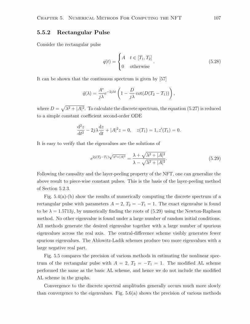
Chapter 5. Numerical Methods For Computing the NFT 107
5.5.2 Rectangular Pulse
Consider the rectangular pulse
q(t) =
A t ∈ [T1, T2]
0 otherwise. (5.28)
It can be shown that the continuous spectrum is given by [57]
q(λ) =A∗
jλe−2jλt
(1− D
jλcot(D(T2 − T1))
),
whereD =√λ2 + |A|2. To calculate the discrete spectrum, the equation (5.27) is reduced
to a simple constant coefficient second-order ODE
d2z
dt2− 2jλ
dz
dt+ |A|2z = 0, z(T1) = 1, z′(T1) = 0.
It is easy to verify that the eigenvalues are the solutions of
e2j(T2−T1)√λ2+|A|2 =
λ+√λ2 + |A|2
λ−√λ2 + |A|2
. (5.29)
Following the causality and the layer-peeling property of the NFT, one can generalize the
above result to piece-wise constant pulses. This is the basis of the layer-peeling method
of Section 5.2.3.
Fig. 5.4(a)-(b) show the results of numerically computing the discrete spectrum of a
rectangular pulse with parameters A = 2, T2 = −T1 = 1. The exact eigenvalue is found
to be λ = 1.5713j, by numerically finding the roots of (5.29) using the Newton-Raphson
method. No other eigenvalue is found under a large number of random initial conditions.
All methods generate the desired eigenvalue together with a large number of spurious
eigenvalues across the real axis. The central-difference scheme visibly generates fewer
spurious eigenvalues. The Ablowitz-Ladik schemes produce two more eigenvalues with a
large negative real part.
Fig. 5.5 compares the precision of various methods in estimating the nonlinear spec-
trum of the rectangular pulse with A = 2, T2 = −T1 = 1. The modified AL scheme
performed the same as the basic AL scheme, and hence we do not include the modified
AL scheme in the graphs.
Convergence to the discrete spectral amplitudes generally occurs much more slowly
than convergence to the eigenvalues. Fig. 5.6(a) shows the precision of various methods

Chapter 5. Numerical Methods For Computing the NFT 108
-2
-1
0
1
2
-100 -50 0 50 100
ℑ(λ)
ℜ(λ)
-2
-1
0
1
2
-100 -50 0 50 100
ℑ(λ)
ℜ(λ)(a) (b)
-2
-1
0
1
2
-100 -50 0 50 100
ℑ(λ)
ℜ(λ)
-2
-1
0
1
2
-100 -50 0 50 100
ℑ(λ)
ℜ(λ)(c) (d)
Figure 5.4: Discrete spectrum of the rectangular pulse (5.28) with A = 2, T2 = −T1 = 1using (a) Fourier method, (b) central difference method, (c) Ablowitz-Ladik scheme, (d)modified Ablowitz-Ladik scheme.
10−4
10−3
10−2
0 200 400
e
N
CDAL1SP
10−5
10−4
10−3
10−2
10−1
0 200 400
e
N
10−5
10−4
10−3
10−2
10−1
0 200 400
e
N
FDRK
LPCNAL1
(a) (b)
Figure 5.5: Error in estimating the largest eigenvalue of the rectangular pulse q(t) =2rect(t) as a function of the number of sample points N using (a) matrix-based methodsand (b) search-based methods.

Chapter 5. Numerical Methods For Computing the NFT 109
2.8
3.2
3.6
44.2
0 400 800 1200
q
N
FDRKCNLP
AL1 0
0.6
1.2
1.8
-15 -10 -5 0 5 10 15
|q(λ)|
λ(a) (b)
Figure 5.6: (a) Convergence of the discrete spectral amplitude for the rectangular pulseq(t) = 2rect(t) as a function of the number of sample points N . Factor −j is not shownin the figure. (b) Continuous spectrum.
in estimating the discrete spectral amplitude of the rectangular wave with A = 2, T2 =
−T1 = 1. It can be seen that convergence does not occur until N > 1000. Fig. 5.6(b)
shows the continuous spectrum for the same function. All methods produced essentially
the same continuous spectrum, except for some very slight variations near zero frequency.
As |A| is increased, more eigenvalues appear on the imaginary axis. The distance be-
tween these eigenvalues becomes smaller as |λ| is increased. All methods produce similar
results, with the Ablowitz-Ladik methods reproducing the purely imaginary eigenvalues
at spurious locations with large real part. Phase addition has no influence on any of
these methods, as expected analytically.
5.5.3 N-Soliton Pulses
We consider an 4-soliton pulse with discrete spectrum
q(−1 + 0.25j) = 1, q(1 + 0.25j) = −j,q(−1 + 0.5j) = −1, q(1 + 0.5j) = j. (5.30)
The 4-soliton is generated by solving the Riemann-Hilbert linear system of equations
with zero continuous spectrum [57] and can be seen in Fig. 5.7(a). Figs. 5.8(a)-(d) show
the discrete spectrum of the signal using various matrix-based methods. The relative
accuracy of these schemes in estimating the eigenvalue λ = 1+0.5j is shown in Fig. 5.7(b).
A very similar graph is obtained for other eigenvalues. Iterative methods fare similarly

Chapter 5. Numerical Methods For Computing the NFT 110
0
0.5
1
1.5
2
2.5
-15 -10 -5 0 5 10 15
|q(t)|
t
10−5
10−4
10−3
10−2
10−1
0 400 800 1200
e
N
CDAL1SP
(a) (b)
Figure 5.7: (a) Amplitude profile of a 4-soliton pulse with spectrum (5.30). (b) Error inestimating the eigenvalue λ = 1 + 0.5j.
and their performance is shown in Fig. 5.9(b).
The convergence of the discrete spectral amplitudes q(λj) is not quite satisfactory.
Discrete spectral amplitudes associated with eigenvalues with small |=(λj)| can be ob-
tained with reasonable accuracy, although the convergence of q(λj) is slower than the
convergence of the eigenvalues themselves. On the other hand, discrete spectral ampli-
tudes associated with eigenvalues with large |=(λ)| are extremely sensitive to the location
of eigenvalues and even slight changes in eigenvalues lead to radically different estimates
for the spectral amplitudes. In fact, as the energy of the pulse is increased by hav-
ing eigenvalues with large |=(λ)|, the Riemann-Hilbert system becomes ill-conditioned.
Therefore the discrete spectral amplitudes cannot generally be obtained using the meth-
ods discussed in this chapter. It is illustrative to see the surface of |a(λ)| in Fig. 5.21.
The eigenvalues sometimes correspond to deep and narrow wells in the surface of |a(λ)|,and sometimes they correspond to flat minima. In cases that they correspond to narrow
wells, the derivative a′(λ) is sensitive to the location of eigenvalues, leading to sensitivities
in q(λj). It is also clear from (5.18) that a′(λ) is proportional to λ2 and thus is sensitive
to λ.
Note that q(λj) do not appear in the trace formula, and in particular they do not
contribute to the signal energy. This part of the NFT controls the time center of the
pulse and influences the signal phase too. Due to dependency on the time center of the
signal and the fact that time center can hardly be used for digital transmission, the values
of q(λj) appear to be numerically chaotic and cannot carry much information. For this
reason, we do not discuss these quantities in detail.
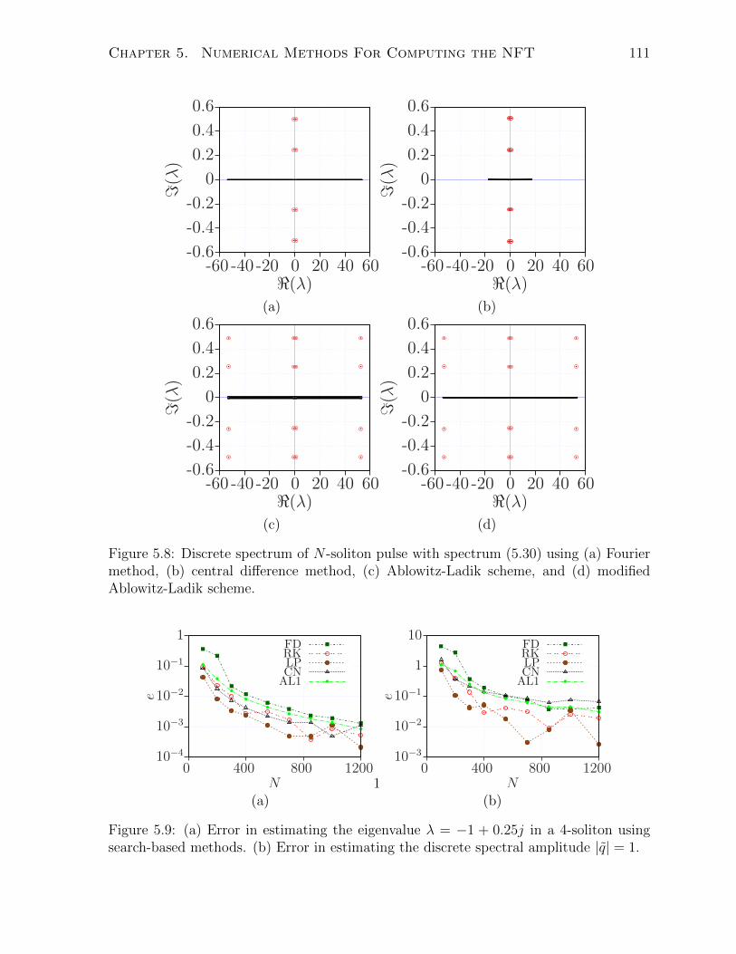
Chapter 5. Numerical Methods For Computing the NFT 111
-0.6
-0.4
-0.2
0
0.2
0.4
0.6
-60 -40 -20 0 20 40 60
ℑ(λ)
ℜ(λ)-0.6
-0.4
-0.2
0
0.2
0.4
0.6
-60 -40 -20 0 20 40 60
ℑ(λ)
ℜ(λ)(a) (b)
-0.6
-0.4
-0.2
0
0.2
0.4
0.6
-60 -40 -20 0 20 40 60
ℑ(λ)
ℜ(λ)-0.6
-0.4
-0.2
0
0.2
0.4
0.6
-60 -40 -20 0 20 40 60
ℑ(λ)
ℜ(λ)(c) (d)
Figure 5.8: Discrete spectrum of N -soliton pulse with spectrum (5.30) using (a) Fouriermethod, (b) central difference method, (c) Ablowitz-Ladik scheme, and (d) modifiedAblowitz-Ladik scheme.
10−4
10−3
10−2
10−1
1
0 400 800 1200
e
N
FDRKLPCNAL1
1
10−3
10−2
10−1
1
10
0 400 800 1200
e
N
FDRKLPCNAL1
(a) (b)
Figure 5.9: (a) Error in estimating the eigenvalue λ = −1 + 0.25j in a 4-soliton usingsearch-based methods. (b) Error in estimating the discrete spectral amplitude |q| = 1.

Chapter 5. Numerical Methods For Computing the NFT 112
0
0.2
0.4
0.6
0.8
1
1.2
-4 -2 0 2 4
|q(λ)|
λ
0
1
−1 0 1
ℑ(λ)
ℜ(λ)
0
1
2
3
-4 -2 0 2 4
|q(λ)|
λ
0
1
−1 0 1
ℑ(λ)
ℜ(λ)
(a) (b)
0
5
10
15
20
-4 -2 0 2 4
|q(λ)|
λ
0
1
−1 0 1
ℑ(λ)
ℜ(λ)
0
10
20
30
-8 -4 0 4 8
|q(λ)|
λ
0
1
−1 0 1
ℑ(λ)
ℜ(λ)
(c) (d)
Figure 5.10: Nonlinear Fourier transform of a sinc function with amplitude A = 1, 2, 3, 4.
5.6 Nonlinear Fourier Transform of Pulses in Data
Communications
In this section, we use the numerical methods discussed in Section 5.1 to compute the
nonlinear Fourier transform of signals typically used in optical fiber transmission. The
emphasis is on sinc functions as they constitute signal degrees of freedom, but we also
consider raised-cosine functions, sech signals, and Gaussian pulses. In particular, we
study the effect of the amplitude and phase modulation on the structure of the nonlinear
spectra. We will also discuss the spectrum of wavetrains formed by sinc functions.
Since the layer-peeling and the spectral methods give accurate results in estimating
the nonlinear spectra, they are chosen for subsequent simulations.

Chapter 5. Numerical Methods For Computing the NFT 113
0
1
2
3
-4 -2 0 2 4
ℑ(λ)
ℜ(λ)0
5
10
15
20
-4 -2 0 2 4
ℑ(λ)
ℜ(λ)
(a) (b)
Figure 5.11: Locus of eigenvalues of the sinc function under amplitude modulation: (a)A = 0 to A = 5, (b) A = 0 to A = 20.
5.6.1 Amplitude and Phase Modulation of Sinc Functions
Fig. 5.10 shows the spectrum of y(t) = Asinc(2t) under amplitude modulation. It can
be seen that a sinc function is all dispersive as A is increased from zero, until about
A = π (||q||L1 = 1.2752π) where a new eigenvalue emerges from the origin. Starting
from A = 0, the continuous spectrum is a rectangle, resembling the ordinary Fourier
transform −F(q∗(t))(2λ). As A is increased, the continuous spectral function is narrowed
until A = π, where it looks like a delta function and its energy starts to deviate from
the energy of the time domain signal. As A > π is further increased, the dominant
eigenvalue on the jω axis moves up until A = 1.27π, where λ1 = 1.4234j and a new
pair of eigenvalues emerges, starting from λ23 = ±3.2 + 0.05j. When the newly created
eigenvalues are not pronounced enough, for instance in this example when transiting from
A = π to A = 1.27π, numerical algorithms have difficulties in determining whether these
small emerging eigenvalues are part of the spectrum or not. Here it appears that for
π < A < 1.27π there is just one dominant purely imaginary eigenvalue moving upward.
At A = 1.27π, λ23 emerge and move up in the complex plane as A is increased. An
important observation is that the sinc function appears to have not only purely imaginary
eigenvalues, but also a pair of symmetric eigenvalues with nonzero real part emerging at
high values of A; see Fig. 5.11(b). This means that, for example, a sinc function (viewed
in the time domain) contains a stationary “central component” plus two small “side
components” which travel to the left and right if the sinc function is subject to the NLS
flow. The locus of the eigenvalues of the function Asinc(2t) as a result of variations in A
is given in Fig. 5.11.
It follows that the sinc function is a simple example of a real symmetric pulse whose

Chapter 5. Numerical Methods For Computing the NFT 114
-2
0
2
-4 -2 0 2 4
6q(λ)
λ
-2
0
2
-4 -2 0 2 4
6q(λ)
λ(g) (h)
Figure 5.12: Phase of the continuous spectrum of a sinc function when: (a) A = 4, (b)A = 4j.
0
1
2
3
-5 0 5
|q(λ)|
λ
0
1
2
3
-5 0 5
|q(λ)|
λ
0123
-6 -4 -2 0 2 4 6
ℑ(λ)
ℜ(λ)(a) (b) (c)
Figure 5.13: (a) Amplitude of the continuous spectrum with no carrier. (b) Amplitudeof the continuous spectrum with carrier frequency ω = 5. The phase graph is also shiftedsimilarly with no other change (∆λ = 2.5). (c) Locus of the eigenvalues of a sinc functionwith amplitude A = 8 as the carrier frequency exp(−jωt) varies.
eigenvalues are not necessarily purely imaginary, as conjectured for a long time. However
if q(t) is real, non-negative, and “single-lobe”, then there are exactly N = b12
+||q||L1
π− εc
eigenvalues, all purely imaginary [51].
Under phase modulation, in the form of adding a constant phase term to the signal,
the eigenvalues and the magnitude of the continuous spectrum remained unchanged.
Vertical shift in the phase of the continuous spectrum as a result of phase modulation
can be seen in Fig. 5.12.
We may also examine the effect of time-dependent phase changes. The effect of linear
chirp, of the form exp(jωt), is shown in picture Fig. 5.13. Linear chirp results in just a
shift of the discrete and continuous spectrum to the left or the right, depending on the
sign of the chirp.
It is interesting to observe the effect of a quadratic chirp. The locus of eigenvalues
that result due to changes in the quadratic phase q exp(jωt2) has been studied in [51]
for Gaussian pulses. In our sinc function example, in the case that there is one discrete

Chapter 5. Numerical Methods For Computing the NFT 115
0
1
2
-4 -2 0 2 4
ℑ(λ)
ℜ(λ)0
0.2
0.4
-20 0 20
ℑ(λ)
ℜ(λ)0
5
10
-4 -2 0 2 4
ℑ(λ)
ℜ(λ)(a) (c) (d)
0
5
10
-2 -1 0 1 2
ℑ(λ)
ℜ(λ)0
2
4
6
-4 -2 0 2 4
ℑ(λ)
ℜ(λ)0
2
4
6
-4 -2 0 2 4
ℑ(λ)
ℜ(λ)(b) (e) (f)
Figure 5.14: Eigenvalues of Ae−jωt2sinc(2t): (a) locus of eigenvalues for A = 4 and ω = 0.5
to ω = 50, (b) locus of eigenvalues for A = 12 and ω = 0 to ω = 50, (c) eigenvaluesfor A = 4 and ω = 15, (d) eigenvalues for A = 12 and ω = 0.50, (e) eigenvalues forA = 12 and ω = 41.39 just before collision, (f) eigenvalues for A = 12 and ω = 41.43after collision.
eigenvalue in the chirp-free case (such as when A = 4), increasing ω will move the
eigenvalue on the jω axis upward, but then the eigenvalue move down again and is
absorbed in the real axis. Fig. 5.14(c) shows the moment before the eigenvalue is absorbed
into the real axis. Note that the eigenvalues off the jω axis are considered to be spurious;
their number increases as the number of sample points is increased.
A more interesting behavior is observed when A = 12. Here, there are two eigenvalues
on the jω axis: λ1 ≈ 10.0484j, λ2 = 5.5515j, together with λ3,4 = ±3.1315 + 0.7462j
(Fig 5.14(d)). As ω is increased, λ1 and λ2 move down and a fifth eigenvalue λ5 emerges
from the real axis and moves upwards on the jω axis. Eventually, at about ω = 41.41,
λ2 and λ5 “collide” and move out of the jω axis to the left and right. If ω is further
increased, λ2 and λ5 are absorbed into the real axis; see Fig. 5.14.
Collision of eigenvalues also occurs with time dilation. Signal q(t) = sinc(at) has 3
eigenvalues on the jω axis for a = 0.1, plus two small eigenvalues on two sides of the jω
axis (Fig 5.16(b)). As a is increased, the smaller eigenvalue on the jω axis comes down
and a new eigenvalue is generated at the origin, moving upward. These two eigenvalues
collide at 0.12j (a = 0.1330) and are diverted to the first and second quadrant, and

Chapter 5. Numerical Methods For Computing the NFT 116
0
0.4
0.8
-40 -20 0 20 40
|q(λ)|
λ
ω = 0ω = 10ω = 30
-4
-2
0
2
4
-20 0 20
6q(λ)
λ
A = 1, ω = 10
-4
-2
0
2
4
-20 0 20
6q(λ)
λ
A = 1, ω = 30
(a) (b) (c)
Figure 5.15: (a) Nonlinear spectral broadening as a result of quadratic phase modulationAejωt
2sinc(2t) with A = 1 and ω = 0, 10 and 30. (b) Phase of the continuous spectrum
when A = 1 and ω = 10. (c) Phase of the continuous spectrum when A = 1 and ω = 30.
eventually absorbed in the real axis at about <λ = ±0.32 (ω = 0.1990), Fig. 5.16(c)-
(d)). As a is decreased, more eigenvalues appear on the jω axis and fewer on the real
axis (Fig. 5.16(e)-(f)). Note that the eigenvalues are not necessarily on the jω axis. For
example, the signal y = sinc(0.1370t) clearly has eigenvalues λ1 = 0.8684j, λ2 = 0.5797j,
λ3,4 = ±0.1055 + 0.1210i.
Fig. 5.15 shows the nonlinear spectrum of a sinc pulse under a quadratic chirp mod-
ulation, given by Aejωt2sinc(2t), is broadened as ω varies.
The effect of time dilation on the continuous spectrum can be seen in Fig. 5.17. It
can be observed that increasing bandwidth a, will increase the continuous range of real
nonlinear frequencies, leading to bandwidth expansion.
5.6.2 Sinc Wavetrains
The nonlinear spectrum of a wavetrain can take on a complicated form, just like its
ordinary Fourier transform counterpart. Eigenvalues of a two-symbol train, for instance,
depend on the amplitude and phase of the two signals, and their separation distance.
We first analyze the case in which there are only two sinc functions located at the
fixed Nyquist distance from each other, i.e., y(t) = a1sinc(2t + 12) + a2sinc(2t − 1
2). For
a1 = a2 = 2 the spectrum consists of a single eigenvalue λ = 0.3676j and a number of
spurious eigenvalues as shown in Fig. 5.18(a). As the phase of a2 is increased from θ = 0
to θ = π, the eigenvalues moves off the jω axis to the left and a new eigenvalue emerges
from the real axis in the first quadrant. Eigenvalues at θ = π are ±1.3908+ 0.3287i. The
resulting locus of eigenvalues is shown in Fig. 5.18(b). Figs 5.18(c)-(d) depict similar
graphs when both a1 and a2 change.
Next we study the locus of the discrete spectrum as a function of pulse separation
for fixed amplitudes. If the amplitude of the sinc functions is increased sufficiently,

Chapter 5. Numerical Methods For Computing the NFT 117
-1
-0.5
0
0.5
1
-1 -0.5 0 0.5 1
ℑ(λ)
ℜ(λ)-1
-0.5
0
0.5
1
-0.5 0 0.5
ℑ(λ)
ℜ(λ)(a) (b)
-1
-0.5
0
0.5
1
-0.5 0 0.5
ℑ(λ)
ℜ(λ)-1
-0.5
0
0.5
1
-0.5 0 0.5
ℑ(λ)
ℜ(λ)(c) (d)
-1
-0.5
0
0.5
1
-0.5 0 0.5
ℑ(λ)
ℜ(λ)-1
-0.5
0
0.5
1
-0.5 0 0.5
ℑ(λ)
ℜ(λ)(e) (f)
Figure 5.16: Locus of eigenvalues of sinc(at) as the bandwidth varies (a) from a = 0.1 toa = 0.6. (Eigenvalues with small =λ are not shown here.) (b) Eigenvalues for a = 0.1.(c) Eigenvalues before collision and (d) after collision. (e) Eigenvalues for a = 0.06 beforecollision and (f) for a = 0.065 after collision.

Chapter 5. Numerical Methods For Computing the NFT 118
0
2
4
6
-0.5 0 0.5
|q(λ)|
λ
a = 0.06a = 0.1a = 0.3
0
1
2
-4 -2 0 2 4
|q(λ)|
λ
a = 1a = 2a = 3
(a) (b)
Figure 5.17: Bandwidth expansion in sinc(at) for (a) a = 0.06, a = 0.1, a = 0.3 (b)a = 1, a = 2, a = 3.
0
0.2
0.4
-5 0 5
ℑ(λ)
ℜ(λ)0
0.1
0.2
0.3
0.4
0.5
-4 -2 0 2 4
ℑ(λ)
ℜ(λ)(a) (b)
0
1
2
3
4
5
-4 -2 0 2 4
ℑ(λ)
ℜ(λ)0
1
2
3
4
5
-4 -2 0 2 4
ℑ(λ)
ℜ(λ)(c) (d)
Figure 5.18: Discrete spectrum of y(t) = a1sinc(2t− 12) + a2sinc(2t+ 1
2) for (a) a1 = a2,
(b) a1 = 2, a2 = 2ejθ for −π < θ ≤ π, (c) a1 = 2, 0 ≤ a2 ≤ 6, (d) a1 = 4j, 0 ≤ a2 ≤ 6.

Chapter 5. Numerical Methods For Computing the NFT 119
eigenvalues appear off the real axis and form a locus as the distance between pulses varies.
Fig. 5.19(a) shows the locus of eigenvalues of y(t) = 4sinc(2t + τ) + 4sinc(2t − τ) as τ
changes between zero to 5. At τ = 0, eigenvalues are λ1 = 6j, λ2,3 = ±2.3618 + 0.6476i
and λ4,5 = ±3.2429 + 0.0815i. As the distance between pulses is increased, λ1 rapidly
decreases, and at about τ = 0.25, where λ1 = 4.3j, the eigenvalues with non-zero real
parts are absorbed into the real axis at <λ = −3. As τ is further increased, λ1 decreases
further, until τ = 0.4 where λ1 = 2.4j and two new eigenvalues emerge at locations
<λ = ±3.12 going up and towards the jω axis. These eigenvalues return, before reaching
the jω axis, to be absorbed into the real axis, while new eigenvalues are generated again
from the real axis. At τ = 0.7 eigenvalues are λ = 2j, ±1 + j. At some point, the
newly created eigenvalues are not absorbed into the real axis, but they reach the jω
axis and collide. A collision occurs, for instance, at τ = 1.05. One of these eigenvalues
goes down to be absorbed into the origin, and the other one, interestingly, goes up to be
united with the maximum eigenvalue on the jω axis (i.e., to create one eigenvalue with
multiplicity two). Increasing the distance further does not change the location of this
eigenvalue, which from now is fixed at λ = 1.4j, but just changes the pattern of lower
level eigenvalues. The collision does not occur when the amplitudes of the signals are
smaller; see Fig. 5.19 (b) for the locus of the eigenvalues when the amplitude of the two
sinc functions is 2.
0
1
2
3
4
5
-4 -2 0 2 4
ℑ(λ)
ℜ(λ)0
0.5
1
1.5
-4 -2 0 2 4
ℑ(λ)
ℜ(λ)(a) (b)
Figure 5.19: (a) The locus of the discrete spectrum of y(t) = 4sinc(2t+ τ) + 4sinc(2t− τ)as a function of 0 ≤ τ ≤ 5. (b) The locus of the discrete spectrum of y(t) = 2sinc(2t +τ) + 2sinc(2t− τ) as a function of 0 ≤ τ ≤ 5.
For wavetrains with a larger number of signals, the number of eigenvalues increases
proportionally. We generate these wavetrains randomly and examine the region to which
the spectrum is confined. Fig. 5.20 shows the locus of the discrete spectrum of all sinc
wavetrains with 16 signals. All 16 signal degrees of freedom in the bandlimited signal are

Chapter 5. Numerical Methods For Computing the NFT 120
modulated here. The effect of the bandwidth constraint in the nonlinear spectral domain
can seen in this picture.
0
2
4
-4 -2 0 2 4ℑ(
λ)
ℜ(λ)
Figure 5.20: Effect of the bandwidth constraint on the location of the eigenvalues of asinc wavetrain containing 16 pulses having random amplitudes.
5.6.3 Preservation of the Spectrum of the NLS Equation
It is crucial to ensure that the spectrum found by the numerical methods, such as those
discussed in the previous sections, is in fact correct. While it proved difficult to do so
consistently and efficiently, there are various tests to increase one’s confidence in the truth
of the output of the numerical methods. Taking the inverse nonlinear Fourier transform
in the continuous-time domain and comparing the resulting function in time with the
original signal is generally quite cumbersome and not always feasible. One quick test
is to examine a time frequency identity, such as the trace formula for n = 1, 2, 3, . . . as
used in this chapter. The first few conserved quantities in this identity can be written
explicitly. One should allow higher tolerance values in the trace formula for large n, as the
discrete terms in this identity involve λn and thus are increasingly more sensitive to the
eigenvalues. Another test is to subject the signal to the flow of an integrable equation,
such as the NLS equation, and check that the discrete spectrum is preserved and the
spectral amplitudes are scaled appropriately according to that equation. In this section,
we let the signal propagate according to the NLS equation and compare the spectra at
z = 0 and z = L for various L.
Fig. 5.21 shows examples of the spectra of a number of pulses at z = 0 and z = Levolving according to the NLS equation (5.1). The distances mentioned in the graphs in
km correspond to a standard optical fiber with parameters in Table 2.1.
Note that in all these examples discrete the spectrum is completely preserved, and the
continuous spectral amplitudes undergo a phase change properly. Compared to Gaussian
and raised-cosine examples, whose nonlinear Fourier transform can be found easily, the

Chapter 5. Numerical Methods For Computing the NFT 121
(a)1
2
3
-15 15
|q(t)|
t
z = 0 kmz = 1000 kmz = 5000 km
0
1.5
3
-2 -1 0 1 2
|q(λ)|
λ
0
1
2
-1 0 1
ℑ(λ)
ℜ(λ)
z = 0 kmz = 1000 kmz = 5000 km
−50
5
05
100
0.5
1
ℜ(λ)ℑ(λ)
|a(λ
)|
(b)
1
2
3
-4 -2 0 2 4
|q(t)|
t
z = 0 kmz = 1000 kmz = 2000 kmz = 3000 km
0
7.5
15
-1 0 1
q(λ)|
λ
0
2
-1 0 1
ℑ(λ)
ℜ(λ)
z = 0 kmz = 1000 kmz = 2000 kmz = 3000 km
−50
5
02
40
0.5
1
ℜ(λ)ℑ(λ)
|a(λ
)|
(c)2
4
6
-30 -20 -10 0 10 20 30
|q(t)|
t
z = 0 kmz = 1000 kmz = 2000 kmz = 4000 km
0
5
10
-10 -5 0 5 10
|q(λ)|
λ
0
2
4
-1 0 1
ℑ(λ)
ℜ(λ)
z=0 kmz=1000 kmz=2000 kmz=4000 km
−50
5
05
100
0.5
1
ℜ(λ)ℑ(λ)
|a(λ
)|
(d)1
2
-20 -10 0 10 20
|q(t)|
t
z = 0 kmz = 500 kmz = 1000 kmz = 2000 km
0
1
2
-4 -2 0 2 4
|q(λ)|
λ
0
1
-1 0 1
ℑ(λ)
ℜ(λ)
z=0 kmz=500 kmz=1000 kmz=2000 km
−50
5
02
40
0.5
1
ℜ(λ)ℑ(λ)
|a(λ
)|
Figure 5.21: Propagation of pulses along an optical fiber in the time domain (left), in thenonlinear Fourier transform domain (middle), and showing the surface of |a(λ)| (right).The pulses are (a) Gaussian pulse, (b) Satsuma-Yajima pulse, (c) raised-cosine pulse, (d)sinc pulse. The zeros of |a(λ)| correspond to eigenvalues in C+.
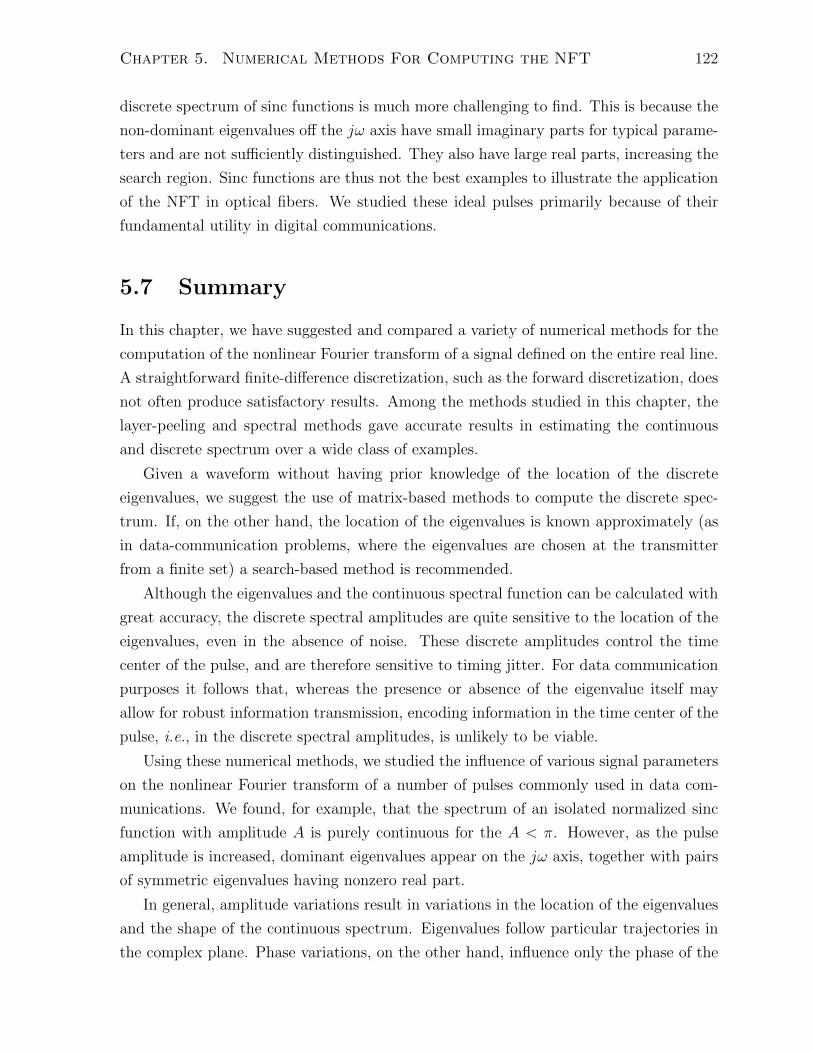
Chapter 5. Numerical Methods For Computing the NFT 122
discrete spectrum of sinc functions is much more challenging to find. This is because the
non-dominant eigenvalues off the jω axis have small imaginary parts for typical parame-
ters and are not sufficiently distinguished. They also have large real parts, increasing the
search region. Sinc functions are thus not the best examples to illustrate the application
of the NFT in optical fibers. We studied these ideal pulses primarily because of their
fundamental utility in digital communications.
5.7 Summary
In this chapter, we have suggested and compared a variety of numerical methods for the
computation of the nonlinear Fourier transform of a signal defined on the entire real line.
A straightforward finite-difference discretization, such as the forward discretization, does
not often produce satisfactory results. Among the methods studied in this chapter, the
layer-peeling and spectral methods gave accurate results in estimating the continuous
and discrete spectrum over a wide class of examples.
Given a waveform without having prior knowledge of the location of the discrete
eigenvalues, we suggest the use of matrix-based methods to compute the discrete spec-
trum. If, on the other hand, the location of the eigenvalues is known approximately (as
in data-communication problems, where the eigenvalues are chosen at the transmitter
from a finite set) a search-based method is recommended.
Although the eigenvalues and the continuous spectral function can be calculated with
great accuracy, the discrete spectral amplitudes are quite sensitive to the location of the
eigenvalues, even in the absence of noise. These discrete amplitudes control the time
center of the pulse, and are therefore sensitive to timing jitter. For data communication
purposes it follows that, whereas the presence or absence of the eigenvalue itself may
allow for robust information transmission, encoding information in the time center of the
pulse, i.e., in the discrete spectral amplitudes, is unlikely to be viable.
Using these numerical methods, we studied the influence of various signal parameters
on the nonlinear Fourier transform of a number of pulses commonly used in data com-
munications. We found, for example, that the spectrum of an isolated normalized sinc
function with amplitude A is purely continuous for the A < π. However, as the pulse
amplitude is increased, dominant eigenvalues appear on the jω axis, together with pairs
of symmetric eigenvalues having nonzero real part.
In general, amplitude variations result in variations in the location of the eigenvalues
and the shape of the continuous spectrum. Eigenvalues follow particular trajectories in
the complex plane. Phase variations, on the other hand, influence only the phase of the

Chapter 5. Numerical Methods For Computing the NFT 123
spectrum, not the location of the eigenvalues. One important observation, which may be
beneficial for the design of data communication systems, is that the nonlinear spectrum
of bandlimited pulses appears to be confined to a vertical strip in the complex plane with
a width proportion to the signal bandwidth.
This chapter has only scratched the surface of a potentially rich research area. The
development of efficient and robust numerical techniques suitable for various engineering
applications of the nonlinear Fourier transform will require significant additional effort. A
problem of particular interest is the development of a “fast” nonlinear Fourier transform
method that would be the analog of the FFT.

Chapter 6
Discrete and Continuous Spectrum
Modulation
Few things are harder to put up with
than a good example.
Mark Twain
In the previous chapters it was suggested to exploit the integrability and use the non-
linear Fourier transform to transmit information over integrable communication channels,
such as the optical fiber channel. In this transmission scheme information is encoded in
the nonlinear Fourier transform of the signal, consisting of a discrete and a continuous
spectral function. In this chapter, we provide further detail on the nonlinear spectrum
modulation and determine gains achievable via modulating the spectral invariants of the
nonlinear Schrodinger equation. Since the guard time between pulses can be large in
a dispersive system, a large number of discrete spectral degrees of freedom should be
eventually modulated. This corresponds to an implementation of the inverse nonlinear
Fourier transform from a suitably chosen 2N complex discrete spectral degrees of free-
dom to an N -soliton pulse in time domain. We examine various ways to generate such
N -solitons for N 1 for nonlinear transmission over optical fiber networks. The result-
ing method compatible with the channel nonlinearity can have significant potential for
long-haul fiber data transmission.
After describing the structure of the NFT transmitter, we give some examples show-
ing how to use the nonlinear Fourier transform for data transmission, improving upon
the classical soliton systems. The nonlinear Fourier transform of a signal with respect
to a Lax operator consists of discrete and continuous spectral functions, in one-to-one
correspondence with the signal [57]. In this chapter, we mostly consider the important
124

Chapter 6. Discrete and Continuous Spectrum Modulation 125
special case where the continuous spectrum is zero, examining data transmission schemes
conceived by modulating the discrete spectrum.
An important step in developing a communication theory of waveform channels is
to appropriately discretize the channel and identify a suitable set of degrees of freedom.
The NFT provides a means to discretize integrable nonlinear dispersive waveform chan-
nels. The proposed nonlinear frequency-division multiplexing (NFDM) scheme can be
considered as a generalization of orthogonal frequency-division multiplexing (OFDM) to
integrable nonlinear dispersive communication channels. The advantages of NFDM arise
from the following:
1. NFDM removes inter-channel interference (cross-talk) between users of a network
sharing the same fiber channel;
2. NFDM removes inter-symbol interference (ISI) (intra-channel interactions) for
each user;
3. spectral invariants as carriers of data are remarkably stable and noise-robust fea-
tures of the NLS flow;
4. with NFDM, information in each channel of interest can be conveniently read
anywhere in a network without knowledge of the distance or any information
about other users.
Modulating the discrete spectrum corresponds to multisoliton transmission and detec-
tion. Fiber-optic communications using fundamental solitons (i.e., 1-solitons) has faced
numerous challenges in the past decades. The spectral efficiency of current soliton sys-
tems is typically quite low. Solitons interact with each other and in the presence of noise
the system-reach is limited by the Gordon-Haus effect [69]. Despite solutions suggested
to alleviate these limitations [69], the industry currently considers the use of more tradi-
tional pulse-shapes, such as sinc and raised-cosine pulses, which may not be particularly
compatible with the structure of the nonlinear Schrodinger (NLS) equation [39], which
governs pulse transmission in optical fibers.
This chapter improves upon the classical soliton systems by using multisoliton pulse
shapes as carriers of data. While a fundamental soliton can be modulated, detected and
analyzed in the time domain, multisolitons are best understood via their nonlinear spec-
trum in the complex plane. In this chapter, these pulses are obtained by implementing
a simplified inverse NFT at the transmitter, and are demodulated at the receiver by
recovering their spectral invariants using the forward NFT. Numerical methods for the
calculation of the forward NFT are discussed in Chapter 5. Here we discuss the inverse
NFT for the case that the continuous spectrum is zero.
It can be observed numerically that the discrete spectrum of a long random wavetrain,

Chapter 6. Discrete and Continuous Spectrum Modulation 126
e.g., that formed from a sinc basis, appears to contain most of the wavetrain energy.
This implies that a sample function from a stationary bandlimited stochastic process
x(t), −T/2 < t < T/2 is approximately a multisoliton as T → ∞. The fact that a
large class of input signals of interest are indeed multisolitons implies that the desirable
properties of such signals (or issues such as interactions and timing jitters) exist to the
same extent for multisolitons and, in fact, are better understood in the context of the
latter. Since parameters of a multisoliton naturally do not interact with one another,
there is potentially a great advantage in directly modulating these parameters. Sending
an N -soliton train for large N and detecting it at the receiver with the help of the NFT,
the interaction of the individual components is no longer problematic.
There is a vast body of literature on solitons in mathematics, physics, and engineer-
ing; see, e.g., [9, 10, 69] and references therein. Classical, path-averaged and dispersion-
managed fundamental 1-solitons are well-studied in fiber optics [69]. The existence of
optical N -soliton pulses in optical fibers is also well known [69]. These results however
mostly study the pulse propagation properties of an N -soliton pulse, are usually limited
to small N (e.g. N = 2, 3), and consider specific isolated input signals (e.g., inputs of
the form Asech(t)). Since N -solitons are naturally defined in the nonlinear spectral do-
main, in general they are best decoded with the help of the nonlinear Fourier transform.
With the exception of few papers, we are aware of no other work using soliton trains or
the nonlinear Fourier transform for data transmission. See [45] for an early interesting
work on multi-solitons and the inverse scattering transform and [70] for a more recent
(in progress) publication. The general viewpoint taken in this chapter is similar to that
of [45].
6.1 Background
6.1.1 System Model
As before, we consider a standard single-mode (SSM) fiber with dispersion coefficient β2,
nonlinearity parameter γ and length L. We thus consider again the normalized stochastic
NLS equation (3.3) of Chapter 4, with parameters given in Table 2.1. We do not perform
dispersion compensation, although the NLS equation is integrable for both positive and
negative dispersions.

Chapter 6. Discrete and Continuous Spectrum Modulation 127
6.1.2 The Discrete Spectral Function
Here we briefly recall the definition of the discrete spectral function in the context of
the nonlinear Schrodinger equation. We first consider the deterministic version of (3.3),
where the noise is zero. Later, we will treat noise as a perturbation of the noise-free
equation.
The nonlinear Fourier transform of a signal in (3.3) arises via spectral analysis of the
operator
L = j
(∂∂t
−q(t)−q∗(t) − ∂
∂t
)= j (DΣ3 +Q) , (6.1)
where D = ∂∂t
,
Q =
(0 −q−q∗ 0
), and Σ3 =
(1 0
0 −1
).
Let v(t, λ) be an eigenvector of L with eigenvalue λ. Following Chapter 4, the discrete
spectral function of the signal propagating according to (3.3) is obtained by solving the
the Zakharov-Shabat eigenproblem Lv = λv, or equivalently
vt =
(−jλ q(t)
−q∗(t) jλ
)v, v(−∞, λ) =
(1
0
)e−jλt, (6.2)
where the initial condition was chosen based on the assumption that the signal q(t)
vanishes as |t| → ∞. The system of ordinary differential equations (6.2) is solved from
t = −∞ to t = +∞ to obtain v(+∞, λ). The nonlinear Fourier coefficients a(λ) and b(λ)
are then defined as
a(λ) = limt→∞
v1(t, λ)ejλt,
b(λ) = limt→∞
v2(t, λ)e−jλt.
Finally, the discrete spectral function is defined on the upper half complex plane C+ =
λ : =(λ) > 0:
q(λj) =b(λj)
a(λj), j = 1, · · · , N,
where λj are the isolated zeros of a(λ) in C+, i.e., solutions of a(λj) = 0. The continuous
spectral function is defined on the real axis λ ∈ R as q(λ) = b(λ)/a(λ).
Chapter 6. Discrete and Continuous Spectrum Modulation 128
6.2 Modulating the Discrete Spectrum
Let the nonlinear Fourier transform of the signal q(t) be represented by
q(t)←→ (q (λ), q(λj)) .
When the continuous spectrum q(λ) is set to zero, the nonlinear Fourier transform con-
sists only of discrete spectral functions q(λj), i.e., N complex numbers λ1, . . . , λN in
the upper half complex plane C+ together with the corresponding N complex spectral
amplitudes q(λ1), . . . , q(λN). In this case, the inverse nonlinear Fourier transform can be
worked out in closed-form, giving rise to N -soliton pulses [71]. The resulting expressions,
however, quickly get complicated when N > 2. As a consequence, analytical results tend
to be limited to low-order solitons.
One can, however, create and modulate these multisolitons numerically. In this section
we study various schemes for the implementation of the inverse NFT at the transmitter
when q = 0.
6.2.1 Discrete Spectrum Modulation by Solving the Riemann-
Hilbert System
The inverse nonlinear Fourier transform can be obtained by solving a Riemann-Hilbert
system of integro-algebraic equations or, alternatively, by solving the Gelfand-Levitan-
Marchenko integral equations. Great simplifications occur when q(λ) is zero. For in-
stance, in this case the integral terms in the Riemann-Hilbert system vanish and the
integro-algebraic system of equations is reduced to an algebraic linear system, whose
solution gives rise to N -soliton pulses.
Let V (t, λj) and V (t, λ∗j) denote the scaled eigenvectors associated with λj and λ∗j de-
fined by their boundary conditions at +∞ (they are denoted by V 1 and V 1 in Chapter 4).
Setting the continuous spectral function q(λ) to zero in the Riemann-Hilbert system of
Chapter 4, we obtain an algebraic system of equations
V (t, λ∗m) =
(1
0
)+
N∑
i=1
q(λi)e2jλitV (t, λi)
λ∗m − λi,
V (t, λm) =
(0
1
)−
N∑
i=1
q∗(λi)e−2jλ∗i tV (t, λ∗i )
λm − λ∗i. (6.3)

Chapter 6. Discrete and Continuous Spectrum Modulation 129
Define
V2×N =(V (t, λ1) V (t, λ2) · · · V (t, λN)
),
V2×N =(V (t, λ∗1) V (t, λ∗2) · · · V (t, λ∗N)
),
KN×N =
q1e2jλ1t
λ∗1−λ1
q1e2jλ1t
λ∗2−λ1· · · q1e2jλ1t
λ∗N−λ1
q2e2jλ2t
λ∗1−λ2
q2e2jλ2t
λ∗2−λ2· · · q2e2jλ2t
λ∗N−λ2
......
. . ....
qNe2jλN t
λ∗1−λNqNe
2jλN t
λ∗2−λN· · · qNe
2jλN t
λ∗N−λN
,
(J1)2×N =
(1 1 · · · 1
0 0 · · · 0
),
(J2)2×N =
(0 0 · · · 0
1 1 · · · 1
),
eN×1 =(
1 1 · · · 1)T
,
J2×N = J2 − J1K∗ =
(−eTK∗
e
),
FN×1 =(q1e
2jλ1t q2e2jλ2t · · · qNe
2jλN t)T
.
In this notation, the algebraic equations (6.3) are simplified to
V = J1 + VK V = J2 − VK∗. (6.4)
Note that K∗ is the complex conjugate of K (not Hermitian). Therefore
V = (J2 − J1K∗) (IN + KK∗)−1 = J (IN + KK∗)−1 ,
and V2 = eT (IN + KK∗)−1. The N -soliton formula is given by
q(t) = −2jeT (IN + K∗K)−1 F∗. (6.5)
The right hand side is a complex scalar and has to be evaluated for every t to determine
samples of q(t) everywhere.
Example 12. It is useful to see the (scaled) eigenvectors for a single soliton with spectrum

Chapter 6. Discrete and Continuous Spectrum Modulation 130
q(α+jω2, z) = q0e
2αωze−j(α2−ω2)z and the eigenvector
v(t, λ; z) =1
2sech[ω(t− t0)]
(e−jΦ
eω(t−t0)
), (6.6)
where Φ = αt+ (α2 − ω2)z −∠q0 − π2
and t0 = 1ω
log |q0|ω− 2αz. The celebrated equation
for the single soliton obtained from (6.5) is
q(t) = −jωe−jαte−jφ0sech (ω(t± t0)) . (6.7)
From the phase-symmetry of the NLS equation, the factor −j in (6.7) can be dropped.
The real and imaginary part of the eigenvalue are the frequency and amplitude of the
soliton. Note that the discrete spectral amplitude q(λ) is responsible for the phase and
time-center of the soliton.
6.2.2 Discrete Spectrum Modulation via the Hirota Bilineariza-
tion Scheme
It is also possible to generate multisolitons without solving a Riemann-Hilbert system
or directly using the NFT. A method which is particularly analytically insightful is the
Hirota direct method [71]. It prescribes in some sense a nonlinear superposition for
integrable equations.
The Hirota method for an integrable equation works by introducing a transforma-
tion of the dependent variable q to convert the original nonlinear equation to one or
more homogeneous bilinear PDEs. For integrable equations, the nonlinearity usually is
canceled or separated out. The resulting bilinear equations have sum of exponentials so-
lutions. Computationally, bilinear equations are solved perturbatively by expanding the
unknowns in terms of the powers of a small parameter ε. For integrable equations, this se-
ries truncates, rendering approximate solutions of various orders to be indeed exact. The
bilinearization transformation has been found for many integrable equations [71], taking
on similar forms that usually involve the derivatives of the logarithm of the transformed
variable.
Let us substitute q(t, z) = G(t,z)F (t,z)
, where, without loss of generality, was may assume
that F (t, z) is real-valued. To keep track of the effect of nonlinearity, let us restore the
nonlinearity parameter γ in the NLS equation. Plugging into the resulting NLS equation
jqz = qtt + 2γ|q|2q,

Chapter 6. Discrete and Continuous Spectrum Modulation 131
we get
j (GzF − FGz) = FGtt − 2FtGt −GFtt+ 2
F 2t + γ|G|2
FG
= FGtt − 2FtGt +GFtt
+ 2F 2t + γ|G|2 − FFtt
FG, (6.8)
where we have added and subtracted 2GFtt. Equation (6.8) is trilinear in F and G. It
can be made bilinear by setting
j(GzF −GFz) = FGtt − 2FtGt +GFtt,
F 2t + γ|G|2 − FFtt = 0. (6.9)
It is very convenient (though not necessary) to organize (6.9) using the Hirota D operator
Dnt (a(t), b(t)) =
(∂
∂t− ∂
∂t′
)na(t)b(t′)|t=t′ ,
as
(jDz +D2t )FG = 0, (6.10)
D2tFF = 2γ|G|2. (6.11)
Note that the D-operator acts on a pair of functions to produce another function.
Note further that (6.10) does not depend on the nonlinearity parameter γ. That is to
say, the nonlinearity has been separated from equation (6.10). For some other integrable
equations (e.g., the Korteweg-de Vries equation for which one gets only one bilinear
PDE), the nonlinearity parameter is in fact canceled completely.
Because (6.10) and (6.11) are homogeneous in the order of derivatives that occur in
each term, exponential functions are candidate solutions. This suggests that F and G
can be expanded (linearized) as
F (t, z) = f 0(t, z) + εf (1)(t, z) + ε2f (2)(t, z) + · · · ,G(t, z) = g0(t, z) + εg(1)(t, z) + ε2g(2)(t, z) + · · · ,

Chapter 6. Discrete and Continuous Spectrum Modulation 132
for some small parameter ε. We then obtain
FG = f (0)g(0) + ε(f (0)g(1) + f (1)g(0)
)
+ ε2(f (0)g(2) + f (1)g(1) + f (2)g(0)
)+ · · · ,
F 2 = (f (0))2 + 2εf (0)f (1) + ε2(
2f (0)f (2) + f (1)2
+)
+ · · · ,|G|2 = |g(0)|2 + ε
(g(0)g(1)∗ + g(0)∗g(1)
)
+ ε2(g(0)g(2)∗ + g(2)g(0)∗ + |g(1)|2
)+ · · · ,
which can then be substituted into (6.10)-(6.11). Equating like powers of ε, one obtains
bilinear equations for sub-components f (i)g(j) using the D operator. As shown below (for
the NLS), this series truncates for integrable systems and exact solutions of various finite
order are obtained. To begin finding unknowns recursively, we can set initially f (0) = 1.
The zero-order term in (6.10) gives jg(0)z + g
(0)tt = 0 or g(0) = ceX0 , where X0 =
2jλ0t− k0z+φ0. Here λ0 = (α+ jω)/2 is the eigenvalue, k0 = 4jλ20, and φ0 is a constant
phase related to the spectral amplitude (φ0 = log(q/ω2)). The zero-order term in (6.11)
gives c = 0, and thus g(0) = 0. At this stage, we can set the higher order terms to zero
and get the trivial solution q = 0.
The ε term in (6.10) gives g(1) = αeX1 . The corresponding term in (6.11) gives
2D2t f
(1) = 0, or f (1) = 0.
The ε2 term in (6.11) is D2t f
(2) = 2|g(1)|2, or 2f(2)tt = 2|g(1)|2. Trying f (2) = αeX1+X∗1 ,
we get α = (λ− λ∗)−2/4. At this stage, we can set other higher order unknowns to zero
and get the one soliton solution (choosing ε = 1)
F (t, z) = 1 +1
4(λ− λ∗)2eX1+X∗1 ,
G(t, z) = eX1 ,
q(t, z) =
(e−X1 +
1
4(λ− λ∗)2eX∗1
)−1
= ωsech [ω (t− 2αz − t0)] ejαt−j(α2−ω2)z.
where t0 = log(|q|/ω)/ω.
We can continue to find higher order solitons. The ε2 term in (6.10), i.e., (jDz +
D2t )1.g2 = 0, gives g2 = α2e
X2 .

Chapter 6. Discrete and Continuous Spectrum Modulation 133
In general, we have
F (t, z) =∑
m=0,1
D1(m) exp(m · x + mTΦm
),
G(t, z) =∑
m=0,1
D2(m) exp(m · x + mTΦm
),
where m = [mi]2Ni=1, mi = 0, 1, x = [Xi]
2Ni=1, Xi = ωit−kiz+Xi(0), ki = jωi, Xi+N = X∗i ,
Φ = [φij]2Ni,j=1,
φij =
0 i ≥ j
−2 log (ωi + ωj)i=1,2,··· ,N
j=N+1,N+2,··· ,2N
−2 log (ωi − ωj) i=N+1,··· ,2Nj=N+1,N+2,··· ,2N
and
D1(m) =
1N∑i=1
mi =N∑i=1
mi+N
0 otherwise
,
D2(m) =
1N∑i=1
mi = 1 +N∑i=1
mi+N
0 otherwise
.
Note that, using the identity ∂tt logF =FttF−F 2
t
F 2 , (6.11) is reduced to |q(t, z)|2 =
γ−1∂tt logF . The amplitude of q is thus captured by the real-valued function F , while G
contains the phase of the signal.
Two important observations follow from the Hirota method. Firstly, multisoliton
solutions of the NLS equation in the F ,G domain (q = G/F ) are the summation of
exponentially decaying functions β(α)e−αtejωt, each located at a frequency ω. That is to
say, while plane waves ej(ωt−kz) are the natural basis functions that solve linear PDEs,
for integrable systems, exponentially decaying functions are suitable. The addition of the
decaying factor e−αt (when t > 0) is the point at which the nonlinear Fourier transform
diverges from the linear Fourier transform [58]. Secondly, for each individual soliton
term, the Hirota method adds two-way interaction terms, three-way interaction terms,
etc., until all the interactions are accounted for. In this way, the interference between
individual components is removed, as shown schematically in Fig. 6.1. Tables 6.1 and

Chapter 6. Discrete and Continuous Spectrum Modulation 134
b1b2bN−1bN
bk to ak
mapper
and
modulator
· · · · · ·F
interaction
terms
G
interaction
terms
GFe−aN−1te+jωN−1t
e−a2te+jω2t
e−a1te+jω1t
e−aN te+jωN t
q(t)
Figure 6.1: (a) Hirota modulator in creating N -solitons.
Table 6.1: The structure of the interaction terms in F .F
N = 1 1 + eX1+X∗1
N = 2 1 + eX1+X∗1 + eX2+X∗2 + eX1+X∗2 + eX2+X∗1
N = 3 1 + eX1+X∗1 + eX2+X∗2 + eX3+X∗3 +(eX1+X∗2 + eX2+X∗1 + eX1+X∗3 + eX3+X∗1 + eX2+X∗3 + eX3+X∗2
)+(
eX1+X2+X∗1 +X∗2 + eX1+X2+X∗1 +X∗3 + eX1+X2+X∗2 +X∗3 + eX1+X3+X∗1 +X∗2 + eX1+X3+X∗1 +X∗3 + eX1+X3+X∗2 +X∗3)
(+eX2+X3+X∗1 +X∗3 + eX2+X3+X∗1 +X∗2 + eX2+X3+X∗2 +X∗3
)+ eX1+X2+X3+X∗1 +X∗2 +X∗3
6.2 show these interaction terms for N = 1, 2, 3.
While the Hirota method reveals important facts about the structure of the NLS
equation, it may not be the best method to compute multisolitons numerically. There
are(
2NN
)∼ 22N and
(2NN+1
)∼ 22N terms in F and G respectively, and unless one truncates
the interaction terms at some step, the complexity quickly grows, making it hard to
compute N -solitons for N ≥ 10.
6.2.3 Recursive Discrete Spectrum Modulation Using Darboux
Transformation
Multisoliton solutions of the NLS equation can be constructed recursively using the Dar-
boux transformation (DT). The Darboux transformation, originally introduced in the

Chapter 6. Discrete and Continuous Spectrum Modulation 135
Table 6.2: The structure of the interaction terms in G.G
N = 1 eX1 + eX∗1
N = 2 eX1 + eX∗1 + eX1+X2+X∗1 + eX1+X2+X∗2
N = 3 eX1 + eX2 + eX3 +(eX1+X2+X∗1 + eX1+X2+X∗2 + eX1+X2+X∗3 + eX1+X3+X∗1 + eX1+X3+X∗2 + eX1+X3+X∗3
)(eX2+X3+X∗1 + eX2+X3+X∗2 + eX2+X3+X∗3
)+(eX1+X2+X3+X∗1 +X∗2 + eX1+X2+X3+X∗2 +X∗3 + eX1+X2+X3+X∗2 +X∗3
)
v (t, λk+1; q(t;λ1, · · · , λk))
q(t;λ1, · · · , λk)
q(t;λ1, · · · , λk+1)
v (t, µ; q(t;λ1, · · · , λk))
v(t, λk+1; q(t;λ1, · · · , λk)
v(t, µ; q(t;λ1, · · · , λk+1)
(a) (b)
Figure 6.2: (a) Signal update. (b) Eigenvector update.
q(t) = 0
v(t, λ1; 0)
v(t, λ2; 0)
v(t, λ3; 0)
· · ·
v(t, λN−2; 0)
v(t, λN−1; 0)
v(t, λN ; 0)
q(t;λ1)
v(t, λ2; q(t;λ1))
v(t, λ3; q(t;λ1))
v(t, λ4; q(t;λ1))
· · ·
v(t, λN−1; q(t;λ1))
v(t, λN ; q(t;λ1))
q(t;λ1, λ2)
v(t, λ3; q(t;λ1, λ2))
v(t, λ4; q(t;λ1, λ2))
v(t, λ5; q(t;λ1, λ2))
· · ·
v(t, λN ; q(t;λ1, λ2))
· · ·
· · ·
· · ·. ..
q(t;λ1, λ2, · · · , λN−1)
v(t, λN ; q(t;λ1, λ2, · · · , λN−1))
q(t;λ1, · · · , λN )
Figure 6.3: Darboux iterations for the construction of an N -soliton.
context of the Sturm-Liouville differential equations and later used in the nonlinear in-
tegrable systems, provides the possibility to construct from one solution of an integrable
equation another solution [72]. For instance, one can start from the trivial solution q = 0
of the NLS equation, and recursively obtain all higher order N -soliton solutions. This
approach is particularly suited for numerical implementation.
Let x(t, λ; q) denote a solution of the system
xt = P (ζ, q)x,
xz = M(ζ, q)x, (6.12)
Chapter 6. Discrete and Continuous Spectrum Modulation 136
for the signal q and complex number ζ = λ (not necessarily an eigenvalue of q), where
the P and M operators were defined in Chapter 4. It is clear that x = [x∗2,−x∗1]T satisfies
(6.12) for ζ → ζ∗, and furthermore, by cross-elimination, q is a solution of the integrable
equation underlying (6.12).
The statement of the Darboux theorem is as follows.
Theorem 11 (Darboux Transformation). Let φ(t, λ; q) be a known solution of (6.12),
and set Σ = SΓS−1, where S = [φ(t, λ), φ(t, λ)] and Γ = diag(λ, λ∗). If v(t, µ; q) satisfies
(6.12), then u(t, µ; q) obtained from the Darboux transform
u(t, µ; q) = (µI − Σ) v(t, µ; q), (6.13)
satisfies (6.12) for
q = q − 2j(λ∗ − λ)φ∗2φ1
|φ1|2 + |φ2|2. (6.14)
Furthermore, both q and q satisfy the integrable equation underlying the system (6.12).
Proof. See Appendix D.
The Darboux transform thus provides a means to construct from one solution of an
integrable equation q, another solution q according to (6.14). Theorem 11 immediately
provides the following observations.
1. From φ(t, λ; q) and v(t, µ; q), we can obtain u(t, µ; q) according to (6.13). If µ
is an eigenvalue of q, then µ is an eigenvalue of q as well. Furthermore, since
u(t, µ = λ; q) = 0, λ is also an eigenvalue of q. It follows that the eigenvalues of q
are the eigenvalues of q together with λ, i.e., λ is added to the eigenvalues of q.
2. q is a new solution of the NLS equation obtained from q, and u(t, µ; q) is one of
its eigenvectors.
These observations suggest a two-step iterative algorithm to generate N -solitons
pulses, as illustrated in the Figs. 6.2-6.3. Denote a k-soliton pulse with eigenvalues
λ1, λ2, · · · , λk by q(t;λ1, λ2, · · · , λk) := q(k).
Eigenvector update:
v1(t, λj, q(k+1)) = −
(λj − λk+1)|v1(t, λk+1, q
(k))|2 + (λj − λ∗k+1)|v2(t, λk+1, q(k))|2
v1(t, λj, q
(k))
+(λ∗k+1 − λk+1)v1(t, λk+1, q(k))v∗2(t, λk+1, q
(k))v2(t, λj, q(k)), (6.15)

Chapter 6. Discrete and Continuous Spectrum Modulation 137
v2(t, λj, q(k+1)) = −
(λj − λ∗k+1)|v1(t, λk+1, q
(k))|2 + (λj − λk+1)|v2(t, λk+1, q(k))|2
v2(t, λj, q
(k+1))
−(λk+1 − λ∗k+1)v∗1(t, λk+1, q(k))v2(t, λk+1, q
(k))v1(t, λj, q(k)), (6.16)
for k = 1, · · · , N and j = k, · · · , N .
Signal update:
q(k+1) = q(k) − 2j(λ∗k+1 − λk+1)× v1(t, λk+1, q(k))v∗2(t, λk+1, q
(k))
||v(t, λk+1, q(k))||2. (6.17)
Note that v(t, λj, q(k+1)) can also be obtained directly by solving the Zakharov-
Shabat system for q(k+1). It is however more efficient to update the required eigen-
vector from (6.15)-(6.16). N -solitons can be constructed from the trivial solution q = 0.
The first column of Fig. 6.3 is chosen to be the (non-canonical eigenvector) v(t, λj) =
[Ae−jλjt, Bejλjt]T and iterations are initialized from these vectors to find all k−solitons,
k ≤ N . The coefficients A and B control the spectral amplitudes and the shape of the
pulses. For a single soliton A = exp(j∠q) and B = |q|.
6.3 Evolution of the Discrete Spectrum
Recall that the imaginary and real parts of the eigenvalues correspond, respectively, to
soliton amplitude and frequency. If the real part of the eigenvalue <λ is zero, the N -
soliton does not travel (with respect to a traveling observer) while propagating. The
individual components of an N -soliton pulse with non-zero frequencies travel in retarded
time with speeds proportional to <λi (frequency).
The manner of N -soliton propagation thus depends on the choice of the eigenvalues.
An N -soliton signal is essentially composed of N single solitons coupled together, similar
to a molecule which groups a number of atoms. If the discrete spectrum of the signal lies
completely on the imaginary axis, the pulse preserves its shape or periodically oscillates
during the evolution. If the eigenvalues have non-zero real parts, various components
travel at different speeds and eventually when z →∞ the N -soliton decomposes into N
separate solitons
q(t, z)→∑
ωie−j(αit+kiz+φ0)sech(ωi(t− ti − αiz)),
where λ = (αi + jωi)/2 is the eigenvalue, ki = (α2i − ω2
i )/2, and ti is the time center.
This breakdown of a signal to its individual components, while best observed in the case
of multisolitons, is simply a result of group velocity dispersion and exists for all pulses

Chapter 6. Discrete and Continuous Spectrum Modulation 138
similarly. The extent of breakdown and shift depends on a variety of factors, such as
launch power, length of the fiber, number of mass points, fiber dispersion, and dispersion-
management schemes. If dispersion is not managed, the effects of pulse broadening must
be carefully considered.
6.4 Demodulating the Discrete Spectrum
To demodulate a multisoliton pulse, the eigenproblem (6.2) needs to be solved. There
is limited work in the mathematical literature concerning the numerical solution of the
Zakharov-Shabat spectral problem (6.2). In Chapter 5, we have suggested methods
by which the nonlinear Fourier transform of a signal may be computed numerically.
In particular, here we use the layer-peeling and Ablowitz-Ladik methods described in
Chapter 5 to estimate the discrete spectrum.
Recall that the layer-peeling method works by approximating q(t) as a piece-wise
constant signal and using the layer-peeling property of the nonlinear Fourier transform
mentioned in [37]. Let q(t) be defined in the interval [T1, T2]. The layer-peeling iteration
is given as
a[k + 1] = a[k]x[k]− b[k]y[k],
b[k + 1] = a[k]y[k] + b[k]x[k].
where
x[k] =
(cos(εD)− j λ
Dsin(εD)
)ejλε, (6.18)
y[k] =−q∗kD
sin(Dε)e−2jλt, (6.19)
and x[k](λ) = x∗[k](λ∗), y[k](λ) = y∗[k](λ∗), D =√λ2 + |q[k]|2.
The layer-peeling scheme can be used along with the Newton-Raphson method to
search for the eigenvalues of q(t) in the upper-half complex plane C+. The reader is
referred to Chapter 5 for further details.
6.5 Statistics of the Spectral Data
Unfortunately, the generalized NLS equation that includes an additive space-time noise
term is generally not integrable. The addition of noise also disturbs the vanishing or

Chapter 6. Discrete and Continuous Spectrum Modulation 139
periodic boundary conditions usually assumed in the development of the nonlinear Fourier
transform. However, since the amplified spontaneous emission noise in optical fibers is
quite small compared to the signal level for SNR >10 dB , one can treat the effects of
noise as a small perturbation of the signal, and still safely use the NFT.
Calculation of the exact statistics can be quite cumbersome. This is essentially be-
cause the NLS equation with additive noise, unlike the noise-free equation, has little or no
structure, giving rise to complicated variational representations for the noise statistics.
Even if such exact results are available, they are poorly suited for data communications
studies. One can however approximate or bound these statistics using a perturbation
theory, or simulate them on a computer.
Remark 11. In the special case that the noise is real and multiplicative and only a
function of distance, i.e., the signal is multiplied by a real-valued multiplicative random
variable at each (discrete) point in the fiber, the resulting equation is still integrable and
the theory of the nonlinear Fourier transform can be used with no approximation. We
conjecture that exact statistics of the spectral data can be found in this case.
Remark 12. Note that the generalized NLS equation that includes a loss term is also not
integrable. Note, however, that loss is traded with the distributed Raman amplification
noise, and once including perturbations resulting from the noise, the effect of the fiber
loss can approximately be ignored (though the nature of these two perturbations are
different).
Noise can be added in a discrete or continuous manner. In the case of the discrete
(lumped) noise addition resulting from the erbium-doped fiber amplifiers, the randomness
is on initial conditions and, assuming a finite time interval, the NFT is exact whether
the input pulse is deterministic or random. We refer to this type of the stochasticity
where the randomness comes from the initial conditions and not the medium as the
homogeneous randomness.
If noise is injected continuously throughout the fiber as a result of distributed Raman
amplification (DRA), one has a non-homogeneous noise. Here we can discretize the fiber
into a large number of small fiber segments and add lumped noise at the end of each
segment. The injected noises act as random perturbations of the initial data at the input
of each segment. The DRA can thus be approximately treated similar to the lumped noise
case. This is justified in the view that when simulating the stochastic NLS equation, the
step size in the split-step Fourier method can be as large as the distance between EDFA
amplifiers, i.e., the dynamic of the pulse propagation under DRA and a large number
of EDFAs is about the same. Other non-homogeneous distortions can also be treated
similarly.

Chapter 6. Discrete and Continuous Spectrum Modulation 140
In this section, we study the effect of the these two types of perturbations on the
NFDM channel model. We assume that the noise vanishes, or is negligible, as |t| → ∞and has a finite energy such that the signal remains absolutely integrable almost surely.
6.5.1 Homogeneous Noise
The NFT arises in the spectral analysis of the L operator (6.1). We can easily analyze
the perturbations of the eigenvalues λ as a result of the changes in the signal q(t).
Let us denote the noise-free nonlinear Fourier transform of q(t) by (q(λ), q(λj)). As
the signal q(t) is perturbed to q(t) + εN(t) for some small parameter ε and (normalize)
noise process N(t), the (discrete) eigenvalues and spectral amplitudes slightly deviate
from their nominal values. Separating the signal and noise terms, the perturbed v and λ
satisfy
(L+ εR)v = λv, R =
(0 N
−N∗ 0
), (6.20)
where R is the noise matrix. The study of the stochastic nonlinear Fourier transform
is thus a perturbation theory of the non-self-adjoint operator (6.20). Here we need to
measure the variation of the eigenvalues and eigenvectors as the operator L is changed
from L to L+ εR.
Perturbation theory of Hermitian operators is well-studied in the quantum mechanics
(e.g., by E. Schrodinger). The Zakharov-Shabat operator (6.20) is however non-self-
adjoint. Unfortunately most useful properties of the self-adjoint operators do not carry
to the non-self-adjoint operators, particularly due to the lack of a complete orthonormal
basis. Thus the perturbation of the spectral data for the NLS equation is more difficult
than that for the KdV equation. In both cases (deterministic) perturbation analysis of
the IST already exists in the literature [73–76]. These are however mostly deterministic
results and the distribution of the scattering data is still lacking in the literature. A very
interesting work is [77] in which authors calculate the distribution of the spectral data for
the special case that channel has no noise and the input is a white Gaussian stochastic
process.
Since in this Section we are only interested in finding the noise in eigenvalues (and not
discrete spectral amplitudes whose perturbation analysis can be complicated), a simple
small noise approximation, given below, is sufficient.
For the non-self adjoint operators L, the orthogonality that we require is between the
space of left and right eigenvectors of L associated with distinct eigenvalues; that is to

Chapter 6. Discrete and Continuous Spectrum Modulation 141
say, between eigenvectors of L associated with λ and eigenvectors of the adjoint operator
L∗ associated with µ 6= λ∗. Let us equip the space of eigenvectors with the usual L2 inner
product
〈u, v〉 =
∞
−∞
(u1v∗1 + u2v
∗2) dt. (6.21)
It can be easily verified that the operator Σ3L is self-adjoint, i.e., 〈u,Σ3Lv〉 = 〈Σ3Lu, v〉,where Σ3 = diag(1,−1) is the Pauli matrix.
We use a small noise approximation method, expanding unknown variables in noise
level ε [24] as
v(t) = v(0)(t) + εv(1)(t) + ε2v(2)(t) + · · · (6.22)
λ = λ(0) + ελ(1) + ε2λ(2) + · · · . (6.23)
We assume these variables are analytic functions of ε so that above series are convergent
(without the need to renormalize [24]). Plugging (6.22)-(6.23) into (6.20) and equating
the like powers of ε, we obtain
Lv(0) = λ(0)v(0), (6.24)
(L− λ(0))v(1) = −(R− λ(1))v(0), (6.25)
(L− λ(0))v(2) = −(R− λ(1))v(1) + λ(2)v(0), (6.26)... .
The first term gives that v(0) and λ(0) are eigenvalue and eigenvector of the (nominal)
operator L. To eliminate v1 from the second equation, we take the inner product on both
sides of (6.24) with some vector u; the left hand side of the resulting expression is
〈u, (L− λ(0))v(1)〉 = 〈(L− λ(0))∗u, v(1)〉 = 〈(L∗ − λ(0)∗)u, v(1)〉. (6.27)
To have (6.27) vanish, we can choose u to be an eigenvector of the adjoint operator L∗
associated with an eigenvalue µ = λ(0)∗, i.e., (L∗ − λ(0)∗)u = 0. Since L∗(q) = L(−q),if Lv = λ(0)v, it can be verified that L∗u = λ(0)u for u = [v1,−v2] = Σ3v. Choosing
u := u(0) = Σ3v(0)(t, λ∗)
λ(1) =〈u(0), Rv(0)〉〈u(0), v(0)〉 .

Chapter 6. Discrete and Continuous Spectrum Modulation 142
Using similar calculations we obtain λ(2)
λ(2) =〈u,Rv(1)〉〈u, v(0)〉 − λ
(1) 〈u, v(1)〉〈u, v(0)〉 ,
and so on.
To summarize, the fluctuations of discrete eigenvalues is given by
λn = λn + ε〈un, Rvn〉〈un, vn〉
+O(ε2), n = 1, 2, · · · , N.
It follows that the perturbation of the eigenvalues is distributed, to the first order,
according to a zero mean complex Gaussian distribution.
To find higher order fluctuations of eigenvalues, v(k), k ≥ 1, need to be found as well.
This is done by expanding v(k) in the eigenspace of L associated with all eigenvalues
and using the orthogonality of left and right eigenspaces. Since the operator L is not
self-adjoint under the L2(R) inner product, this calculation is a little more elaborate than
the case that L is self-adjoint (where a complete orthonormal basis exists).
6.5.2 Non-homogeneous Noise and Other Perturbations
Consider the perturbed NLS equation
jQz = Qtt + 2|Q|2Q+ εV (t, z), (6.28)
where ε is a small parameter (noise level), and V (t, z) represents the combined effects of
the signal loss and the distributed noise. Here we will make the a priori assumption that
sample paths of the stochastic process possess sufficient regularity and we do not discuss
the well-posedness properties of (6.28).
Let us represent (6.28) with the same L and M of the noise-free equation and now
let λ vary with time. The equality of mixed derivatives vtz = vzt gives
(−jλz Qz + jQtt + 2j|Q|2Q
−Q∗z + jQ∗tt + 2j|Q|2Q∗ jλz
)v = 0.
This, upon re-arranging and using (6.28), simplifies to
λzv = εRv, R = −R.
Note that, as before, we do not have v(t, z) a priori because, according to (6.1), it

Chapter 6. Discrete and Continuous Spectrum Modulation 143
depends on the noisy signal q(t, z) and λ(z), both of which are unknown. However, if
the noise level ε is small, we can expand v(t, z) and λ in powers of ε as (6.22) and (6.23)
to obtain (λ(0))z = 0 and Rv(0) = (λ(1))zv(0) (i.e., (λ(1))z appears as a time-independent
eigenvalue of R(t)). Taking the inner-product with u(0) = Σ3v(0)(t, λ∗) on both sides of
Rv(0) = (λ(1))zv(0), we obtain the first order variation of eigenvalues
(λ1)z =〈u(0), Rv(0)〉〈u(0), v(0)〉 . (6.29)
It follows from (6.29) that the distribution of deviation of the eigenvalues is approxi-
mately a zero-mean conditionally Gaussian random variable. The variance of this random
variable is signal dependent, and although eigenvectors of an N -soliton can be represented
as a series from Darboux transform, it is best calculated numerically if N ≥ 2.
Example 13. Consider the single soliton of Example 12. It can be verified that 〈Σ3v(t, λ∗), v(t, λ)〉= ω
2(1 + ω2
|q|2 ) = 1ω
, where we assumed |q| = ω so that the soliton is centered at t0 = 0.
Furthermore
〈v(t, λ∗), Rv(t, λ)〉 = −ˆ
(v1(t, λ∗)v∗2(t, λ)N∗ + v2(t, λ∗)v∗1(t, λ)N) dt
= −ˆ
1
2sech(ωt)(v2(t, λ∗) + v∗2(t, λ))<N + j
ˆ1
2sech(ωt)(v2(t, λ∗)− v∗2(t, λ))=Ndt
= −1
2
ˆsech(ωt)<Ndt− j
2
ˆsech(ωt)tanh(ωt)=Ndt,
where N = N exp(jΦ) has the same statistics as N . It follows that
αz = −ˆ
sech(τ)<Ndτ, (6.30)
ωz = −ˆ
sech(τ)tanh(τ)=Ndτ . (6.31)
The Gordon-Haus effect easily follows from the αz equation. Note that in fiber optics
noise is added to the signal, i.e., V → jV .
6.6 Spectral Efficiencies Achievable by Modulating
the Discrete Spectrum
We turn now to the numerical study of N -solition data transmission schemes, providing
simulation results to quantify the gains that are achievable. The baseline system is
assumed to be a classical on-off keying soliton transmission in which in any symbol period
Chapter 6. Discrete and Continuous Spectrum Modulation 144
Ts either zero or a fundamental soliton is sent. To improve upon the classical binary
soliton transmission system, two or more discrete mass points are packed in a time interval
which an on-off keying soliton system occupies, while keeping the bandwidth requirements
same. The location of the eigenvalues and the values of the discrete spectral amplitudes
can be jointly modulated for this purpose. We shall see that the effective useful region in
the upper-half plane to exploit the potential of discrete eigenvalue modulation is limited
by a variety of factors. As noted earlier, in this chapter, we discuss modulating the
continuous spectrum just briefly.
Since modulating the nonlinear spectrum translates to pulses with variable width,
power, and bandwidth, we take the average time, average power, and the maximum
bandwidth to properly convert bits per symbol to bits/s and bits/sec/Hz. We start
by continuously modulating one eigenvalue in a given region (i.e., a classical soliton
with amplitude and phase drawn from a multiple ring constellation). We next consider
multisoliton systems with a number of constellations on eigenvalues and discrete spectral
amplitudes. We compare the achievable spectral efficiencies (and in some cases bit error
rates) with those of an on-off-keyed single-soliton communication system.
Throughout this section, we consider a 2000 km single mode single channel optical
link in which fiber loss is perfectly compensated in a distributed manner using the Raman
amplification. Dispersion compensation is not applied, as it is an advantage of the method
that no dispersion management or nonlinearity compensation is required. We let pulses
interact naturally, as atoms in a molecule, and perform all operations on such groups.
The method however works for dispersion managed fibers as well, and in general with any
operation that does not change integrability. Typical simulation parameters are given in
Table 2.1.
6.6.1 Spectral Efficiency of 1-Soliton Systems
Soliton transmission systems typically do not have high spectral efficiencies. This is
because the amplitude and the width of a single soliton are inversely related, and hence
they require a lot of time or bandwidth per degree of freedom provided. Errors in a soliton
transmission system occur either because of the Gordon-Haus timing jitter effect (which
is the primary source of the error if not managed) or amplitude (energy) fluctuations.
Following the Galilean invariance [9], the Gordon-Haus effect exists for all kind of pulses
to the same extent and is not specific to solitons. This classical effect can be suppressed
with the help of the suitably designed filters, and as a result is ignored in this section.
Let first consider a classical soliton system with only one eigenvalue λ = (α+ jω)/2.

Chapter 6. Discrete and Continuous Spectrum Modulation 145
The joint density fA,Ω(α, ω) can be obtained from (6.30)-(6.31) or just directly by ex-
tracting the dynamics of α and ω from the stochastic NLS equation, resulting to a pair of
coupled stochastic ordinary differential equations. For instance, multiplying the stochas-
tic NLS equation (6.28) by q∗, subtracting from its conjugate, integrating over time, and
using the integration by parts in the dispersion term, we get
∂E
∂z= 2=
∞
−∞
q(τ, z)Z(τ, z)dτ, (6.32)
where E(z) =´|q(τ, z)|2dτ is the energy, and Z = −N∗ is a noise process similar to
N . Thus energy fluctuations is a signal-dependent Gaussian random variable E(z) ∼NR(E(0), σ2
´E(z)dz
)≈ NR(E(0), σ2zE(0)). Ignoring the energy of the continuous
spectrum, we have E ≈ 2ω and
ω(z) = ω(0) + σ
√zω(0)
2NR(0, 1) . (6.33)
The conditional probability density function (PDF) fΩ|Ω0(ω|ω0) is easily derived
f(ω|ω0) =1√
πσ2zω0
e− (ω−ω0)2
σ2zω0 . (6.34)
The the PDF of r =√ω(z) is approximately a Rician distribution
f(r|r0) =r
σ2e−
r2+r202σ2 I0(
rr0
σ2)
≈ 1√2πσ2
e−(r−r0)2
2σ2 , r, r0 ≥ σ, (6.35)
which is signal-independent in high SNRs.
Note that we are interpreting the stochastic NLS equation as a soliton-bearing system
in the limit that noise is small. A soliton of the deterministic NLS equation launched
into a system described by the stochastic NLS equation would have, of course, a growing
continuous spectrum too and, in addition, a very small chance of creating additional
solitons out of noise at some distance, or collapsing into the real axis in the λ plane.
All these effects are negligible if the energy of the launched soliton is large enough and
the propagation distance is not exceedingly long. where the Gaussian approximation is
valid in the limit P σ2. The non-Gaussian part of the PDF could also be taken into
account, however this would be of little value in the evaluation of the capacity as it is
quite negligible and complicates mutual information optimization.

Chapter 6. Discrete and Continuous Spectrum Modulation 146
0
1
2
3
4
5
0 5 10 15 20 25 30
Cbits/symbol
SNR [dB]
Direct detectionSampling at t = 0
NFTNFT HG lower bound
0
0.05
0.1
0.15
0.2
0.25
0.3
0.35
0.4
0.45
0 5 10 15 20 25 30
ρ[bits/s/Hz]
SNR [dB]
Direct detectionSampling at t = 0
NFT
(a) (b)
0
1
2
-0.4 -0.2 0 0.2 0.4
ℑλ
ℜλ
0
1
2
-0.4 -0.2 0 0.2 0.4
ℑλℜλ
(c (d)
Figure 6.4: (a) Capacity (bits/symbol) and, (b) spectral efficiency (bits/s/Hz), of solitonsystems using direct detection, sampling, and the NFT methods. (c) Eigenvalue constel-lation. (d) Noise balls at the receiver in the NFT approach. The signal-dependency ofthe noise balls can be seen e.g., through (6.33).
In [29] we have shown that a half-Gaussian density
f(ω0) =1√2πP
e−ω2
02P , ω0 ≥ 0,
gives the asymptotic capacity for (6.34)
C ∼ 1
2log(1 + SNR )− 1
2,
where SNR = Pσ2 .
Translating capacity in bits/symbol to the spectral efficiency in bits/s/Hz depends
on the receiver architecture. Assuming that the receiver is able to decode pulses with

Chapter 6. Discrete and Continuous Spectrum Modulation 147
variable widths, the spectral efficiency ρ(P) is obtained by
ρ(P) = maxf(ω0)ω0∈S
1
ET (ω0)BW (S)I(ω;ω0),
EP (ω0) ≤ P , (6.36)
where T (ω0) and P (ω0) are the width and the power of a single soliton with amplitude
ω0 and BW (S) = maxω0∈S
BW (ω0) is the maximum passband bandwidth that the signal
set S requires for transmission (set by the minS). For a one soliton signal, we have
approximately
T (ω0) =7
ω0
, P (ω0) =ω2
0
6.2, BW (ω0) = 0.95ω0, (6.37)
where the width T (ω0) includes a guard time, four times the full width at half maximum
power FWHM, so as to minimize the intra-channel interactions.
Using (6.37), the maximum spectral efficiency of a baseline on-off keying system is
obtained to be about ρ ≈ 0.15 bits/s/Hz at the average power P0 = 0.16 mW. Note that
the spectral efficiency problem (6.36) is not convex and hence finding the global optimum
may prove to be challenging. Here we simply optimize mutual information and scale it
by ET (ω)×BWmax(S) evaluated at the capacity achieving input distribution.
Fig. 6.4 shows that capacity and the spectral efficiency of a 1-soliton system with
amplitude modulation using various detection methods. Note that since we do not solve
the optimization problem (6.36), the spectral efficiencies shown in the Fig. 6.4(b) are
only lower bounds to the actual achievable values. Fig. 6.4(c)-(d) shows the transmitted
constellation and the noise balls at the receiver. The actual number of signal levels is
64 in the simulations. Calculation of the approximate capacity is performed using the
Arimoto-Blahut algorithm and is confirmed by numerical interior point optimization.
6.6.2 Spectral Efficiency of 2-Soliton Systems
To illustrate how the NFT method works, we start off by a simple example.

Chapter 6. Discrete and Continuous Spectrum Modulation 148
Modulating Eigenvalues
Consider the following signal set with 4 elements.
S1 : 0,
S2 : q(0.5j) = 1,
S3 : q(0.25j) = 0.5,
S4 : q(0.25j, 0.5j) = (1, 1). (6.38)
We compare this with a standard on-off keying soliton transmission system, consist-
ing of S1 and S2, providing about ρ0 = 0.33 bits/sec/Hz spectral efficiency at P0 =
0.1876 mW and R0 = 7.42 Gbits/sec data rate (see Table. 6.3 and its description). Note
that the noise level is so small compared to the imaginary part of the eigenvalues that
with few eigenvalues performance evaluation is essentially a deterministic analysis.
Table 6.3 shows the energy, duration, power and the bandwidth of the signals in
(6.38). The resulting constellation has the average power 0.46P0 and the average time
duration 1.65T1, where P0 and T1 are power and time duration of the fundamental soliton.
Therefore the new signal sets provides about log 41.65T1W0
= 1.2121 × ρ0 bits/sec/Hz and
operates at R = 1.2121 × R0 for about the same average power (0.5P0). Note that
without S4 the average power would be higher and in addition the improvement in the
spectral efficiency is slightly smaller compared to the on-off keying system. Signal S4 is
the new signal that NFT method adds to what other methods can also include. Signals
such as S4 do not cost much in terms of time × maximum bandwidth product, while
they add additional elements to the signal set. Such additional signals can generally be
decoded only with the help of the nonlinear Fourier transform.
In this example, the receiver needs to estimate the pulse-duration. This can be done
in many ways, e.g., using the NFT computations already performed: zeros of the signal
signal energy duration FWHM 99% duration power bandwidthS1 0 T0 T1 0 W0
S2 E0 T0 T1 P0 W0
S3 0.5 E0 2T0 2T1 0.25P0 0.5W0
S4 1.5 E0 4.25T0 2.58T1 0.58P0 0.5W0
Table 6.3: Parameters of the signal set in Section. 6.6.2. Here E0 = 4×0.5 = 2, T0 = 1.763at FWHM power, T1 = 5.2637 (99% energy), P0 = 0.38 and W0 = 0.5714. The scaleparameters are T ′0 = 25.246 ps and P ′0 = 0.5 mW at dispersion 0.5 ps/(nm− km).

Chapter 6. Discrete and Continuous Spectrum Modulation 149
in time can be detected when [v21ejλt, v2
2e−jλt] reaches a constant value in steady state.
This can be checked at times t = T1, t = 2T1 and t = 2.58T1. If one of the signals is zero
at the end of another signal, one can monitor the energy of the continuous spectrum to
make sure that it is small. If symbol duration is fixed to be the maximum 2.58T1, the
addition of S3 and S4 increases both time interval and cardinality of signal set such that
the spectral efficiency and data rate remained to be same (log(6)/2.58), while operating
at 77% of the on-off keying signal power.
Since solitons with purely imaginary eigenvalues do not suffer from major temporal
or spectral broadening, there would be no major performance loss at the end of the fiber.
Modulating both Eigenvalues and Spectral Amplitudes
We can improve upon the previous example by modulating the spectral amplitudes too.
Consider the following signal set
S1 : 0,
S2 − S5 : q(0.5j) = q1,
S6 − S9 : q(0.25j) = q2,
S10 − S16 : q(0.25j, 0.5j) = (q3, q4). (6.39)
We make a 3-PAM constellation on qi ∈ 0.5, 1, 1.5. This creates a signal set with 16
elements. Here pulses are extended to 3T1 time duration. The resulting constellation has
the average power 1.06P0 and average time duration 2.236T1, where P0 and T1 are power
and time duration of the benchmark on-off keying system. Therefore the new signal set
provides about log 162.236T1W0
= 1.79×ρ0 bits/sec/Hz and operates at R = 1.79×R0 for about
the same average power. If we fix symbol durations to be the maximum 3T1, then the
improvement is ρ = 2.2ρ0 = 0.73 bits/s/Hz, at 80% of the average power.
Again, since real part of the eigenvalues is not modulated, signals do not suffer from
major temporal or spectral broadening, and there would be no performance loss at the
end of the fiber.
Remark 13. Note that modulating the eigenvalues include only the amplitude information
and to excite the other half of the degrees of freedom representing the phase, discrete
spectral amplitudes should be considered too. While |q(λj)| may be noisy, the phase
∠q(λj) or a function of q(λj)j=Nj=1 can be investigated for this purpose. Note however
that the asymptotic behavior of the spectral efficiency can be obtained by considering
the eigenvalues alone.

Chapter 6. Discrete and Continuous Spectrum Modulation 150
6.6.3 Spectral Efficiency of N-Soliton Systems, N ≥ 3
To achieve high spectral efficiencies, a dense constellation in the upper-half complex plane
needs to be considered. A spectral constellation with n eigenvalues in C+ and m levels
for spectral amplitudes provides
log
(n∑
k=0
(n
k
)mk
)= n log (m+ 1) ,
bits. One can continue the argument presented in the previous examples by increasing
n and m. The receiver architecture presented in this thesis is fairly simple and is able
to decode NFT signals rather efficiently. At the transmitter side, one should make sure
that all (m + 1)n signals look good in time and frequency. Some pulses may have a
large peak to average power, bandwidth or (99%) width. We have not found rules
for modulating the spectrum such that the pulses have “good” properties in time too.
While for small examples given here we can check pulse properties directly, in general we
require appropriate ways for selecting the spectral data (specially the discrete spectral
amplitudes).
In this simulation, we assume a constellation with 30 points uniformly chosen in the
interval 0 ≤ λ ≤ 2 on the imaginary axis and create all N -solitons, 1 ≤ N ≤ 6. We
then prune signals with undesirable bandwidth or width from this large signal set. The
remaining multi-solitons are used as carriers of data in the typical fiber system considered
earlier. Here a spectral efficiency of 1.5 bits/s/Hz is achieved. For this calculation, we
take the maximum pulse width (containing 99% of the signal energy) and the maximum
bandwidth of the signal set. Since pulse widths are large, the shift of the signal energy due
to the Gordon-Haus effect is insignificant here. By increasing n and m, the Gordon-Haus
effect is as important as it is for the sinc function transmission and backpropagation.
6.7 Multiuser Communications Using the NFT
As mentioned in Chapter 3, a major gain potentially can potentially be obtained by using
methods which do not suffer from inter-channel interference, such as NFDM. In fact,
interference-free communications is the most promising advantage of the NFT approach.
Recall that the real and imaginary axes of the complex plane in the NFT method
represent, respectively, the signal frequency and amplitude. In a multiuser optical com-
munication system, we partition the complex plane into vertical bins. Each bin contains
one or more degrees of freedom and is assigned to a user. The function of add-drop mul-
Chapter 6. Discrete and Continuous Spectrum Modulation 151
User 0 User 1User -1 · · ·· · ·
<(λ) (frequency)
=(λ) (amplitude)
Figure 6.5: Partitioning C+ for multiuser communication using the NFT.
tiplexers is now modified to multiplex and demultiplex signals in a nonlinear way. Each
nonlinear multiplexer/demultiplexer in principle calculates the spectrum of its input sig-
nal, filters signals which need to be dropped in the complex plane, and specifies the free
bands in the nonlinear spectrum. It then calculates the spectrum of the signals entering
the fiber and puts them in unoccupied bands. Finally, the inverse NFT is taken to output
a time domain signal. This way each user gets a subspace in the complex plane during its
trip in the fiber, operates in that subspace and deterministically does not interfere with
other users. For small peak powers on the imaginary axis, the nonlinear multiplexing is
equivalent to the regular Fourier transform multiplexing and as per-channel powers are
increased, the deviations from the capacity of the linear channels associated with the
prior work is best accounted for.
6.7.1 The Need for a Nonlinear Multiplexer/Demultiplexer
It is a conclusion of this thesis that one needs to multiplex and demultiplex signals in
nonlinear fashion so as to avoid the interference associated with the WDM method and
reach significantly higher spectral efficiencies. The nonlinear frequency-division multi-
plexer described above is complex in the given form and may not be the best description
of a such device (without further simplification). Any multiplexer inducing independent
signal propagation for different users is enough to get to the most of the advantages of the
NFT method. This is true even if the resulting per user channel models are nonlinear.
To find such multiplexer, a deterministic model, as noted in Chapter 3 and advocated in
this thesis, can be considered.

Chapter 6. Discrete and Continuous Spectrum Modulation 152
6.8 Spectral Efficiencies Achievable by Modulating
the Continuous Spectrum
In addition to the discrete spectrum, the continuous spectrum can be modulated too. The
spectrum of an isolated sinc function is purely continuous in low powers, resembling a sinc
function. The continuous spectrum is modulated just like the ordinary Fourier transform
and at the receiver can be estimated with great accuracy. The received spectrum is
then compared with the spectrum of the possible waveforms at the transmitter in the
log-Euclidean norm
d(q2(λ), q1(λ)) =1
π
∞
−∞
log(1 + |q2(λ)− q1(λ)|2
)dλ.
Fig. 6.6(a) shows the capacity of a typical single channel fiber-optic system using the
backpropagation and the nonlinear Fourier transform. The NFT is calculated on a 1024
and 64 point grid on the real axis. The 1024-point NFT can be compared with the 1024-
point FFT implementation of the Split-Step Fourier Method in the backpropagation
scheme. As it can be seen, the NFT and backpropagation methods give about the
same capacities. The slight improvement in the NFT method can be attributed to the
stability of the spectral data compared to the time data (though numerical errors should
be considered too).
Simulation is repeated for 5 WDM channels with the system architecture of Fig. 2.8.
Here, low-pass filters and ROADMs are placed at the end of each fiber segment. The
spectral efficiency in this case is obviously lower due to the inter-channel interference.
Here too, NFT and FFT-based backpropagation produce approximately the same results.
From Fig. 6.6 it follows that at low SNRs NFT and backpropagation give about the
same capacities. As the SNR is increased, the spectral efficiency of the backpropaga-
tion degrades due to ISI (if memory is not accounted for) or inter-channel interference
(inevitably). The spectral efficiency of the NFT is expected to grow further due to the
immunity to the cross talk. We have not yet simulated the spectral efficiency at SNRs
beyond that of Fig. 6.6 due to a large number of simulation variables at high spectral
efficiencies, the introduction of the discrete mass points, and the complexity of the NFT
multiplexer. The major advantage of the NFDM is yet remained to be illustrated.
Note that often the mutual information is rather flat at the location of the capacity-
achieving input distribution. That is to say, the capacity is usually not very sensitive to
the details of the channel. Thus although the stability of the spectral data translates to

Chapter 6. Discrete and Continuous Spectrum Modulation 153
a small improvement in the capacity in low SNRs, the improvements in the probability
of error, as another performance measure, are more substantial in the NFT method.
6.9 Some Remarks
We briefly reiterate few remarks about the NFT method made throughout the thesis to
highlight and recapitulate some of its properties.
Noise in the spectral coordinates The NLS equation with additive noise has no
known integrability structure, in the sense of possessing a set of non-interacting degrees
of freedom, as in the linear or the nonlinear Fourier transform (unless for special cases of
noise). As a result, an additive noise in the time domain gets coordinates in the spectral
domain which are not independent or orthogonal. Since the noise description is signal-
dependent, one gets two kinds of interference in a multiuser nonlinear channel: a large
deterministic interference and a smaller stochastic interference. The NFT method does
not suffer from the large deterministic interference (“strong interference”). However the
smaller stochastic interference is expected to be left over (“weak interference”).
Spectral efficiency of the NFDM method asymptotically As stated above, while
deterministic channels are parallel and independent in the nonlinear Fourier domain, the
presence of the noise correlates degrees of freedom and introduces interference. Thus
NFDM is subject to a weak interference (whose strength depends on the noise level and
SNR).
Note however that the decline of the capacity in the prior work is mostly due to the
(strong) deterministic interference. The stochastic interference is an order of magnitude
smaller and its effects are expected to appear at larger SNRs (of order of the inverse
of the noise power ε−1). As a result, although the spectral efficiency of the NFDM is
expected to be higher and may not peak down at the usual SNRs (∼ 25 dB) where the
spectral efficiency of the WDM transmission and backpropagation declines [7], it too
may ultimately peak down, albeit at much higher SNRs (> 30 dB ). We have not yet
simulated the capacity at such high SNRs to see that at what SNR this may potentially
happen. Such spectral efficiency achievable by the NFDM may be the best achievable
rate, since the channel in the presence of the noise is not known to posses any set of
non-interacting degrees of freedom and thus is fundamentally interference-limited. The
improvements in the spectral efficiency using the NFDM method, compared to the WDM
scheme, can still be significant, due to the immunity to the deterministic interference.

Chapter 6. Discrete and Continuous Spectrum Modulation 154
0
2
4
6
8
10
0 5 10 15 20 25 30 35
Cap
acity[bits/symbol]
SNR [dB]
1024-pt BP1024-pt NFT64-pt NFT
(a)
3
4
5
6
7
8
12 14 16 18 20 22 24 26 28
Cap
acity[bits/symbol]
SNR [dB]
1024-pt BP1024-pt NFT
(b)
Figure 6.6: Capacity of (a) single channel, and (b) WDM optical fiber system using thenonlinear Fourier transform and backpropagation. The SNR is calculated at the systembandwidth and can be adjusted to represent the optical signal-to-noise ratio (OSNR).

Chapter 6. Discrete and Continuous Spectrum Modulation 155
linear(structure)
integrable(structure)
non-integrab
lenon-integrable
2q|q|
α
α = 2
α = 0
Stability
NLSPerturbed NLSLinearized NLS
∂Q(z, t)
∂z+
iβ22
∂2Q(z, t)
∂t2= iγ|Q(z, t)|2Q(z, t) + V (z, t)
absentin NFT
absentin NFT
difficultin NFT
easyin time
difficultin time
difficultin time
(a) (b)
Figure 6.7: (a) As the power of the nonlinearity is increased from α = 0 in jqz =qtt + 2q|q|α, the equation changes from a linear one with structure to a non-integrableequation with no structure, until α = 2 where it becomes integrable and again possessesa (self-organizing) structure. For the purpose of the communications, a channel withstructure is preferred. Thus the near integrable channel in practice (shown by a star)is equalized to an integrable channel (shown by a circle) as in this thesis, or to a linearchannel (shown by a square) as in the prior work. (b) Three terms of the NLS equationin the time and spectral domains.

Chapter 6. Discrete and Continuous Spectrum Modulation 156
This can be seen, for instance, from the capacity simulations performed in [7] which
illustrate that the spectral efficiency of the WDM method vanishes at high SNRs even
if noise is set to zero. This is not the case for the NFDM whose spectral efficiency is
unbounded when the noise is zero. This example shows what gains are expected to be
achievable using the NFDM. It also shows the importance of considering deterministic
models in multi-user optical channels.
Similarities and Differences of NFDM and OFDM
Similarities
1. The degrees of freedom are parallel and independent when noise is zero.
2. As in OFDM, one should consider the NFT under periodic boundary conditions
and obtain a discrete NFT. The development of the discrete NFT already exists
in the mathematics literature [58,78]. A cyclic prefix may be needed at this stage.
Differences
1. Unlike OFDM, the noise in the NFDM method is correlated across spectral com-
ponents and is signal-dependent.
2. Frequencies in the NFDM method are complex numbers. Since discrete frequencies
in C+ come in the form of isolated points as a part of the degrees of freedom, they
can be chosen from a constellation in C+ (e.g., QAM) and are subject to noise
jitter. Thus eigenvalue communication is modulating the (discrete) support of
the nonlinear Fourier transform of the signal (similar to frequency-shift keying).
Modulating the remaining degrees of freedom, i.e., the discrete and continuous
spectral amplitudes, is in analogy with the OFDM.
Some of the Advantages and Disadvantages of the NFT
Advantages Some of the advantages of using the NFDM were mentioned at the
beginning of this chapter (page 122). In short, in this method all deterministic distortions
are zero for all users of a multiple user network (i.e., no SPM, XPM, FWM, ISI or
interference).
Disadvantages
1. NFDM critically relies on the integrability of the channel. Loss, higher order dis-
persion, and other perturbations caused by filters and communication equipments

Chapter 6. Discrete and Continuous Spectrum Modulation 157
not taken into account here contribute to deviations from integrability. There are
however several reasons to believe that the back to back channel from transmitter
to the receiver can still be close to an integrable channel:
(a) NFT is applicable as long as one can see solitons in the fiber. Solitons
have been implemented in practice in the presence of the communication
equipments (filters, multiplexers, analog-to-digital (A/D) converters, etc).
This is an indicator that the back to back channel is still nearly integrable.
(b) With employing Raman amplification the effects of the loss are minimal
(indeed traded with noise perturbation).
(c) Mathematically one has stability results for solitons. A soliton passing
through a filter might be distorted a little, but it re-organizes its shape so
as to revert back to its original shape (or form a soliton living nearby in the
complex plane). For instance as an application of this property, filters were
traditionally used to keep solitons in shape and reduce the Gordon-Haus
timing jitter [69].
(d) In the view that the performance of the WDM method is asymptotically
severed with SNR, the potential gains of using the NFT can be significant.
It may be worthwhile to identify and minimize the perturbations of the
integrability.
(e) The current practice of compensating and equalizing a nearly integrable
channel to make it as linear as possible might be a more significant effort
than making it integrable (see Fig. 6.7 (a)).
2. The nonlinear Fourier coefficients at the receiver are calculated in O(n) operations
per nonlinear frequency, where n is the number of signal samples in time. To
compare with FFT, the complexity of an n-point NFT is O(n2) (fixed number of
Newton steps is assumed in case of discrete frequencies). The complexity of the
transmitter can be even more. As a result, NFT is computationally difficult to
implement or sometimes to simulate.
3. Optical or electrical signal processing of N-solitons and the required hardware for
their nonlinear multiplexing may not be as simple as those in the linear systems.
A signal modulated to have desirable properties in the spectrum may translate
to a signal in the time domain which is not processed easily with the current
technology (e.g., requiring high resolution A/Ds). Note that the NFT decoder
typically requires signal samples at increments smaller than the Nyquist rate. An
interpolation step may be needed to find all the necessary data.
4. Noise in the NFT domain can be difficult to analyze. However given that this

Chapter 6. Discrete and Continuous Spectrum Modulation 158
is the total accumulated noise, and the more important deterministic distortions
are not present in the NFDM, nonlinear spectrum is still a more natural domain
for information-theoretic analysis (see Fig. 6.7 (b)). In the time domain, all three
terms, including the accumulated noise, are difficult to analyze, mainly due to
their interactions.

Chapter 7
Conclusion
A man’s errors are his portals of
discovery.
James Joyce
Motivated by the recent studies showing that the spectral efficiency of optical fiber
networks is severely limited by the impacts of the nonlinearity, we revisited information
transmission in such nonlinear systems. Among numerous distortions, we identified the
inter-channel interference in the multiuser WDM optical networks as the implacable fac-
tor limiting the spectral efficiency at high powers. However this distortion and similar
ones arising from the nonlinearity, are largely due to the use of methods suited for linear
systems, such as pulse train transmission and WDM, for the nonlinear optical channel.
Exploiting the integrability of the NLS equation, we presented a nonlinear frequency-
division multiplexing method which is fundamentally compatible with the structure of
the channel. The distinction with the previous methods is that NFDM is now able to
handle the nonlinearity as well, and thus as the the signal power or transmission distance
is increased, the new method does not suffer from the cross talk between signal compo-
nents, which has severed the performance of the prior work. The scheme has numerous
other advantages desired in a communication network. We took the first steps towards a
communication system implementing the nonlinear Fourier transform. We simplified the
task of the transmitter and receiver and provided examples illustrating how to use the
NFT for data transmission. Although these small examples clearly demonstrate improve-
ments over their benchmark systems, a high spectral efficiency simulation illustrating the
promise of the NFDM that the spectral efficiency does not degrade at moderate SNRs as
in the prior work has not yet been performed. Due to the importance of the nonlinearity
in optical networks, NFT or a similar idea should ultimately be used in the future to
conceive schemes which do not suffer from cross talk or cancel such effects in the existing
systems.
159

Appendices
160

Appendix A
Spectrum of Bounded Linear
Operators
When moving from finite-dimensional spaces (of e.g., matrices) to infinite-dimensional
spaces (of e.g., functions and operators), some results do not carry over necessarily. Here
we recall a few useful results in functional analysis [46].
Let H be a Hilbert space, let D be a dense subset of H, and let L : D → H be an
operator.
Definition 8. The adjoint of L is the operator L∗ whose domain D∗ consists of all ψ ∈ Hfor which there exists an element L∗ψ ∈ H such that
〈L∗ψ, φ〉 = 〈ψ,Lφ〉, ∀φ ∈ D.
The operator L is said to be self-adjoint if D = D∗ and L∗ = L. Ignoring domain
subtleties (as is the case for bounded operators), self-adjoint operators are the analogue
of Hermitian matrices.
Definition 9. Given an operator L on a Hilbert space, an operator M is said to be the
inverse of L if the domain of M is the range of L, the range of M is the domain of L,
and ML = I and LM = I.
We will restrict ourselves now to operators whose D is the entire space H.
An operator L : H → H is invertible if it 1) is one-to-one 2) is onto 3) has bounded
inverse. In finite-dimensional spaces, only the first condition is required.
An operator is bounded if it maps bounded inputs to bounded outputs. A bounded
operator is invertible if it is one-to-one and onto.
161

Appendix A. Spectrum of Bounded Linear Operators 162
Definition 10. The spectrum of an operator L on H is defined as
σ(L) = λ ∈ C|L− λI is not invertible .
The spectrum of a bounded operator can be partitioned into two classes, depending
on the reason that L− λI fails to be invertible.
A complex number λ is considered part of the discrete spectrum if L−λI is not one-to-
one, i.e., Lψ = λψ has a non-zero solution ψ ∈ H. In this case, λ is called an eigenvalue,
and each ψ satisfying this equation for the given λ is an associated eigenvector. The set
of all eigenvalues is called the point spectrum or discrete spectrum of L, σdisc(L).
It can also happen that L − λI fails to be surjective, i.e., the range of L − λI is a
proper subset of H. We call the set of λ for which this happens the continuous spectrum
σcont(L) [46].
In finite-dimensional Hilbert spaces the spectrum is entirely discrete. This may no
longer be true in infinite-dimensional spaces, where the eigenvalues (if they exist) may
only be one part of the spectrum. The spectrum of a self-adjoint operator is real. In
general, σ(L) = σ(L∗).
The following examples illustrate some these possibilities.
Example 14. The operator L(x(t)) = tx(t), x(t) ∈ L2[0, 1], has no eigenvalues and its
spectrum is purely continuous σ(L) = [0, 1].
Example 15. The Fourier transform operator F(q)(ω) =∞
−∞q(t)ejωtdt, regarded as on
operator on L2(R) has the property F4 = I. The eigenvalues are therefore the discrete
values ±1,±j. If p(t) is an arbitrary polynomial, then p(t) exp(−t2/2) is an eigenfunc-
tion.
Example 16. Let ∇2 be the Laplace operator and let r denote the radial distance in the
three-dimensional space. The operator L = −∇2 − 1r
is self-adjoint, and therefore it has
a real spectrum. The continuous spectrum is [0,∞) and the discrete spectrum is given
by λn = − 14n2 , n = 1, 2, . . ..
Example 17. It is possible that the discrete spectrum of an operator is uncountable. For
example, for a sequence (x0, x1, . . .) ∈ `2 = x :∑
i |xi|2 <∞, let the left-shift operator
L be defined as L (x0, x1, x2, . . .) = (x1, x2, . . .). The spectrum consists of the unit disk
|λ| ≤ 1. The portion |λ| < 1 is the discrete spectrum while |λ| = 1 is the continuous
spectrum. The adjoint of L is the right-shift operator R (x0, x1, x2, . . .) = (0, x0, x1, . . .).
This operator has the same total spectrum, but it is entirely continuous.

Appendix A. Spectrum of Bounded Linear Operators 163
Example 18. Consider the Zakharov-Shabat system (4.18), in the form (DI − P )v = 0,
v ∈ L2(R). One can see that for λ ∈ R, the eigenvectors v(t, λ) contain oscillatory terms
exp(±jλt), and thus are not in L2(R) (unbounded in norm). As a result, the operator
(DI−P )−1 is unbounded and the inverse (DI−P )−1 does not exist on the Hilbert space
L2(R). Thus λ ∈ R forms the continuous spectrum. This is generally the case where
for an operator L on H for which the eigenproblem Lv = λv has a solution with infinite
norm.
Note that some authors subdivide what we refer to as the continuous spectrum into
further classes (e.g., residual spectrum, essential spectrum, etc.) [46]; however, for the
purposes of this thesis, classification into discrete and continuous spectra will suffice.
Hermitian matrices are always diagonalizable, have real eigenvalues, and possess a
complete set of orthonormal eigenvectors, which provide a basis for the input space.
There is a perfect generalization of this result to compact self-adjoint operators [46].
Theorem 12 (Hilbert-Schmidt spectral theorem). Let L be a compact self-adjoint op-
erator in H. Then it is always possible to find eigenfunctions ψn of L forming an
orthonormal basis for H.
The spectral theory of operators that are not compact and self-adjoint is more in-
volved; see [46].
An important class of operators are the multiplication operators, which are analogous
to diagonal matrices.
Definition 11 (Multiplication operator). Let f(t) be an arbitrary function. The operator
L defined by (Lψ)(t) = f(t)ψ(t), which performs sample-wise multiplication, is called
the multiplication operator or diagonal operator induced by f(t).
Theorem 13. Every bounded self-adjoint operator in a separable Hilbert space H is
unitarily equivalent to a multiplication operator Γ, i.e., L = UΓU−1 where U is unitary.
It follows that the essence of a bounded self-adjoint operator is just a multiplication
operator.

Appendix B
Riemann-Hilbert Factorization
Problem
B.1 Preliminary
Recall that a complex function f(z) = u(x, y) + jv(x, y) in the complex plane z = (x, y)
is differentiable at a point (x0, y0) if and only if the partial derivatives ux, uy, vx and vy
are continuous and
ux = vy, uy = −vx. (B.1)
The compatibility conditions (B.1) are called the Cauchy-Riemann conditions and are
obtained by equating the limit δz → 0 along the real and imaginary axes. This means
that, unlike real functions, differentiability of a complex function imposes a constraint
between the real and imaginary parts of the function.
A function f(z) is said to be analytic at (x0, y0) if it is differentiable in a neighborhood
of that point. If f(z) is analytic in an open region Ω of the complex plane, then a power
series representation of f(z) is convergent in Ω. Existence of a power series representation
has a number of interesting consequences. For instance, the zeros of a non-zero function
analytic in an open region Ω of C are isolated points in Ω [50].
Lemma 14 (Plemelj formulae). Let C be any smooth, closed, counter-clockwise, contour
in the complex plane and let f(x) be any function satisfying a Holder condition on C
defined by
|f(t)− f(τ)| ≤ k|t− τ |α, k > 0, ∀t, τ ∈ C,
164

Appendix B. Riemann-Hilbert Factorization Problem 165
for some 0 < α ≤ 1. Then the projection integral
F (ζ) =1
2πj
˛
C
f(z)
z − ζ dz, (B.2)
is analytic everywhere in C except possibly at points ζ on the contour C (where F (ζ) is
not defined). If ζ approaches C along a path entirely inside the contour C, then
F+(ζ)∆= lim
z→ζF (ζ) =
f(ζ)
2+
1
2πjp.v.
ˆ
C
f(z)
z − ζ dz. (B.3)
If ζ approaches C along a path entirely outside the contour C, then
F−(ζ)∆= lim
z→ζF (ζ) = −f(ζ)
2+
1
2πjp.v.
ˆ
C
f(z)
z − ζ dz. (B.4)
Here p.v. denotes the principal value integral defined by
p.v.
ˆ
C
f(z)
z − ζ dz = limε→0
˛C−Cε
f(z)
z − ζ dz,
in which Cε is an infinitesimal part of C centered at z = ζ and with length 2ε.
Proof. See [52].
The projected function F (ζ) is a sectionally analytic function of ζ with respect to C,
i.e., it is analytic in sections C+ (the interior of C) and C− (the exterior of C), and the
limits F±(ζ) exist (as given by (B.3) and (B.4)).
A consequence of Lemma 14 is that F±(ζ) satisfies the following jump condition on
the boundary C
F+(t)− F−(t) = f(t).
The projection operator therefore produces functions which are analytic almost every-
where, except on a contour where it experiences a jump in its limits.
B.2 The Scalar Riemann-Hilbert Problem
In the scalar Riemann-Hilbert problem, the task is to find functions f+(z) and f−(z),
analytic, respectively, inside and outside a given smooth closed contour C, such that on

Appendix B. Riemann-Hilbert Factorization Problem 166
C
f+(t) = g(t)f−(t) + h(t) t ∈ C, (B.5)
where h(t) and g(t) (with g(t) 6= 0 for all t ∈ C), are given functions satisfying a Holder
condition on C.
Both unknowns f+(z) and f−(z) can be determined from the single boundary equa-
tion (B.5), using the projection operator (B.2). To see this, first consider the homoge-
neous case where h(t) = 0. One can rewrite (B.5) as a jump condition
log f+(z)− log f−(z) = log g(z) z ∈ C.
Functions log f+(z) and log f−(z) can be viewed as portions of a single sectionally analytic
function log f(z) which is analytic in C+ and C− and on boundary C its limits jump as
log g(t). In view of the projection operator P (B.2), consider
log f(z) =1
2πj
˛
C
log g(λ)
λ− z dλ.
If log g(t) satisfies a Holder condition on C, then log f(z) is analytic strictly inside and
outside C. On C, we can define log f+(z) and log f−(z), respectively, as equal to the
limits (B.3) and (B.4). The function obtained in this way satisfies (B.5) and has the
desired analyticity properties.
Note however that, unlike g(t), log g(t) in the integrand may not satisfy a Holder
condition. To resolve this issue, we can multiply g(t) by a decaying factor t−k, for a
suitable k, to make t−kg(t) Holder, and obtain f+(t) =(t−kg(t)
)(tkf−(z)). Therefore,
defining
F (z) = exp
1
2πj
˛
C
log λ−kg(λ)
λ− z dλ
,
we have the following solution for the homogeneous RH problem:
f+(z) =
F (z) z ∈ C+,
F+(z) z ∈ C,

Appendix B. Riemann-Hilbert Factorization Problem 167
and
f−(z) =
z−kF (z) z ∈ C−,z−kF−(z) z ∈ C.
Here k can be chosen so that t−kg(t) is continuous and the total phase change of log t−kg(t)
is zero along the closed path C.
The solution f±(z) is called the fundamental solution to the scalar RH problem. From
the homogeneity of (B.5), one can obtain other solutions by multiplying f±(z) by any
entire function in C.
We can generalize the above procedure to solve the non-homogeneous Riemann-
Hilbert problem (B.5). In this case, we can find a factorization g(t) = g+(t)g−(t)
by solving
a homogeneous Riemann-Hilbert problem with boundary conditions g+(t) = g(t)g−(t).
Then (B.5) is reduced to
f+(t)
g+(t)− f−(t)
g−(t)=
h(t)
g+(t),
which, as before, can be solved in closed form using the Plemelj formulae.
B.3 The Matrix Riemann-Hilbert Problem
When formulating the inverse nonlinear Fourier transform, we face a matrix Riemann-
Hilbert problem (4.36). Matrix RH problems are generally more involved and may not
allow closed-form solutions [52]. As we will see in the Appendix C.4, for the particular
matrix RH problem (4.36), the projection operator (B.2) is sufficient to solve the problem.

Appendix C
Proofs of Some Results from
Chapter 4
C.1 Proof of Elementary Properties of the NFT
In this section, we sketch the proofs of the properties of the NFT stated in Section 4.3.4.
1. If ||q(t)||L1 1, then y2(t, λ) and q2(t) terms can be ignored in (4.30) and (4.31).
From the resulting equations, it follows that there is no discrete spectrum and
q(λ)→ Q(λ). The quadratic terms are introduced by the NFT to account for the
nonlinearity.
2. This follows from 1) in above, and that when |a| 1, the squared terms repre-
senting the nonlinearity can be ignored.
3. This follows from replacing q(t) with ejφq(t) in (4.30) and (4.31).
4. Scaling the Zakharov-Shabat system (4.18) as t′ = t/a, we obtain the desired
result. Note that if sgn(a) < 0, boundary conditions at ±∞ are interchanged.
5. Property 5) and 6) follow by replacing q(t) with q(t − t0) and e2jωtq(t) in (4.30)
and (4.31), and accordingly changing variables.
6. This is the statement of (4.33).
7. The following identity, known as the trace formula, can be easily proved for the
nonlinear Fourier transform [10]
cn =4
n
N∑
i=1
=(λni ) +1
π
∞
−∞
ζn−1 log(1 + |ρ(ζ)|2
)dζ.
Here cn are the secondary constants of motion, i.e., quantities, directly in terms of
the time domain data, which are preserved during the flow of the NLS equation.
168

Appendix C. Proofs of Some Results from Chapter 4 169
The first few ones are the energy
c1 =
∞
−∞
|q(t)|2dt,
momentum
c2 =1
2j
∞
−∞
q(t)q∗t (t)dt,
and the Hamiltonian
c3 = −∞
−∞
(|q(t)|4 − |qt(t)|2
)dt.
Parseval’s Identity is the trace formula evaluated at n = 1.
8. Let q(t) be supported in the interval [t1, t2] and let K(q(t), t1, t2) denote a propa-
gator (linear transformation) which maps v(t, λ) in (4.18) from v(t1, λ) to v(t2, λ).
The propagator is structured as
K =
(a(λ)ejλ(t2−t1) −b∗(λ∗)ejλ(t2+t1)
b(λ)e−jλ(t2+t1) a∗(λ∗)e−jλ(t2−t1)
).
Let q1(t) and q2(t), supported, respectively, in the intervals [t1, t2] and [t2, t3],
t1 < t2 < t3, correspond to the propagators K1(q1(t), t1, t2) and K2(q2(t), t2, t3).
Then q(t) = q1(t) + q2(t) is supported in [t1, t3], and from linearity corresponds to
the propagator K = K2K1
K =
(a2(λ)ejλ(t3−t2) −b∗2(λ∗)ejλ(t3+t2)
b2(λ)e−jλ(t3+t2) a∗2(λ∗)e−jλ(t3−t2)
)
×(a1(λ)ejλ(t2−t1) −b∗1(λ∗)ejλ(t2+t1)
b1(λ)e−jλ(t2+t1) a∗1(λ∗)e−jλ(t2−t1)
).
The 1× 1 and 2× 1 elements are
K11 = ejλ(t3−t1) (a1(λ)a2(λ)− b1(λ)b∗2(λ∗)) ,
K21 = e−jλ(t3+t1) (a1(λ)b2(λ) + b1(λ)a∗2(λ∗)) .
Comparing with K11 = a(λ)ejλ(t3−t1) and K21 = b(λ)e−jλ(t3+t1), we get the desired

Appendix C. Proofs of Some Results from Chapter 4 170
result.
C.2 Proof of Lemma 10
Analyticity of the canonical eigenvectors is directly a property of the Zakharov-Shabat
system (4.18). Let us scale canonical eigenvectors as V 2 = v2ejλt, V 2 = v2e−jλt,V 1 =
v1e−jλt and V 1 = v1ejλt. Transforming the Zakharov-Shabat system (4.18), the scaled
eigenvectors satisfy
V 2t =
(0 q
−q∗ 2jλ
)V 2, V 2(−∞) =
(1
0
), (C.1)
V 2t =
(−2jλ q
−q∗ 0
)V 2, V 2(−∞) =
(0
1
),
V 1t =
(0 q
−q∗ 2jλ
)V 1, V 1(∞) =
(1
0
),
V 1t =
(−2jλ q
−q∗ 0
)V 1, V 1(∞) =
(0
1
).
Let us, for instance, solve for the canonical eigenvector V 2 in (C.1). Considering the q
terms as an external force and using the Duhamel formula [79], (C.1) can be transformed
into its integral representation
V 2(t, λ) =
(1
0
)
+
∞
−∞
h(t− t′, λ)
(0 q(t′)
−q∗(t′) 0
)V 2(t′, λ)dt′, (C.2)
where the system impulse response h(t, λ) is
h(t, λ) =
(u(t) 0
0 e2jλtu(t)
), (C.3)
and we have ignored transient terms since the boundary condition starts at t = −∞.
The analyticity of eigenvectors can be seen intuitively at at this stage. The impulse
response (C.3) involves the term e2jλtu(t) and hence (C.1) is well defined in C+ if q ∈L1(R). The impulse response for the V 1 equation involves −e−2jλtu(−t) and hence it is
bounded in the same region. The impulse response for V 2 and V 1 have terms proportional

Appendix C. Proofs of Some Results from Chapter 4 171
to e−2jλtu(t) and −e2jλtu(−t), respectively, and therefore these eigenvectors are analytic
in C− for q ∈ L1(R).
A more precise argument proceeds by solving (C.2) explicitly. Duhamel’s integral
(C.2) is of the form of a fixed-point map
V 2 =
(1
0
)+ T (V 2),
where T is the linear operator underlying (C.2). A candidate for the solution is the sum
V 2 =∞∑
k=0
Uk (C.4)
where Uk satisfy the iteration
Uk+1 = T (Uk) +
(1
0
), U0 =
(0
0
).
The first few terms are
U1 =
(1
0
), U2 =
0
−t
t1=−∞q∗(t1)e2jλ(t−t1)dt1
, (C.5)
U3 =
−
t
t2=−∞
t2
t1=−∞q(t2)q∗(t1)e2jλ(t2−t1)dt1dt2
0
, (C.6)
and the kth term is recursively defined by
Uk+1 =
(1
0
)+
tˆ
−∞
(q(t′)Uk
2 (t′, λ)
−q∗(t′)Uk1 (t′, z)e2jλ(t−t′)
)dt′. (C.7)
By induction on k, as (C.7) suggests, if Uk is analytic and q(t) ∈ L1(R), then Uk+1
is analytic. In addition, the series (C.4) is uniformly convergent on t and thus V 2 is
analytic in C+.
Similarly one proves the analyticity of the other canonical eigenvectors in their cor-
responding region.
Appendix C. Proofs of Some Results from Chapter 4 172
C.3 Asymptotics of Canonical Eigenvectors and Non-
linear Fourier Coefficients when |λ| 1
If λ ∈ C+ and |λ| 1, then 1j(ω−2λ)
= −12jλ
+ O(λ−2) and, taking the inverse Fourier
transform, we can approximate e2jλtu(t) = − 12jλδ(t) + O(λ−2). Substituting into (C.4),
(C.5), (C.6), for |λ| 1 we obtain
V 2(t, λ) =
1 + 1
2jλ
∞
−∞|q(t)|2dt
12jλq∗(t)
+O(λ−2). (C.8)
A similar asymptotic expression can be derived for V 1 (λ 1)
V 1(t, λ) =
12jλq(t)
1 + 12jλ
∞
−∞|q(t)|2dt
+O(λ−2).
If |λ| → ∞, q can be assumed zero in (4.18) compared to jλ. Thus v(t, λ) approaches
the boundary conditions at t = ±∞. Therefore
a(λ) = 〈v2(t, λ), v1(t, λ)〉s = 〈v2(+∞, λ), v1(+∞, λ)〉s→ 〈v2(−∞, λ), v1(+∞, λ)〉s = 1. (C.9)
Similarly, it is shown that b(λ)→ 0 as |λ| → ∞.
C.4 Solution of the Riemann-Hilbert Problem in the
NFT
In Section 4.6, the inverse nonlinear Fourier transform was formulated as an instance of
the Riemann-Hilbert factorization problem. Using hints given in the Appendix B, the
resulting factorization problem can be solved in a simplified manner via an appropriate
contour integration.
Dividing both sides of the projection equations (4.24)-(4.25) by a(λ)(λ − ζ), for pa-
rameter ζ ∈ C−, and integrating on the real axis −∞ < λ <∞, we obtain
1
2πj
∞
λ=−∞
V 2(t, λ)
a(λ)(λ− ζ)dλ =
1
2πj
∞
λ=−∞
V 1(t, λ∗)
λ− ζ dλ+1
2πj
∞
λ=−∞
q(λ)e2jλtV 1(t, λ)
λ− ζ dλ, (C.10)
Appendix C. Proofs of Some Results from Chapter 4 173
in which the integration is performed on the open path z = λ,−∞ < λ < ∞. The
integration path thus passes the singularity λ = ζ from above in all the integrals.
Cauchy integrals in (C.10) are computed from the residue theorem. The integration
path −∞ < λ < ∞ can be closed in the upper or lower half-planes. To compute the
first integral, we close the path in the upper half-plane and denote the resulting closed
contour by C+−ζ , i.e., the upper half plane and excluding the singularity z = ζ
1
2πj
∞
λ=−∞
V 2(t, λ)
a(λ)(λ− ζ)dλ =
1
2πj
˛C+−ζ
V 2(t, z)
a(z)(z − ζ)dz − lim
R→∞
1
2πj
Rejπˆ
Rej0
(1
0
)
a(z)(z − ζ)dz
=N∑
i=1
V 2(t, λj)
a′(λj)(λj − ζ)− 1
2
(1
0
)
=N∑
i=1
b(λi)e2jλitV 1(t, λi)
a′(λi)(λi − ζ)− 1
2
(1
0
)
=N∑
i=1
q(λi)e2jλitV 1(t, λi)
λi − ζ− 1
2
(1
0
), (C.11)
where, in the second line, when R → ∞, we have used the asymptotic values (C.8) and
(C.9) in Appendix C.3. Note that we assumed that eigenvalues λj are all simple zeros of
a(λ), i.e., no multiplicity.
To compute the second integral in (C.10), we close the integration path in the lower
half-plane and denote the resulting closed contour by C−+ζ , i.e., the lower half-plane and
including the singularity z = ζ
1
2πj
∞
λ=−∞
V 1(t, λ∗)
λ− ζ dλ =1
2πj
˛C−+ζ
V 1(t, z∗)
z − ζ dz − limR→∞
1
2πj
Rejπˆ
Rej2π
(1
0
)
z − ζ dz
= −V 1(t, ζ) +1
2
(1
0
). (C.12)
The last integral in (C.10) is left uncomputed, because the boundedness of e2jλt
depends on the sign of t. For t > 0, we can consider C+−ζ which leads to the expression
(C.11) multiplied by u(t). For t < 0, we should inevitably consider C−+ζ , where poles of
V 1(x, λ) are unknown. As a result, this integral is left untreated.
Using (C.11) and (C.12) in (C.10), we obtain an integral equation relating canonical

Appendix C. Proofs of Some Results from Chapter 4 174
eigenvectors V 1 and V 1 to q(λ) and q(λj)
V 1(t, ζ∗) =
(1
0
)+
N∑
i=1
q(λi)e2jλitV 1(t, λi)
ζ − λi
+1
2πj
∞
λ=−∞
q(λ)e2jλtV 1(t, λ)
λ− (ζ − jε) dλ. (C.13)
This is the first equation in the Riemann-Hilbert system (4.37) when ζ approaches the
real line from below. Since (C.13) holds for any ζ ∈ C−, evaluating (C.13) at ζ = λ∗j , j =
1, . . . , N , produces the third equation in (4.37). The remaining equations are obtained
by taking the ∼ operation from these two equations and subsequently replacing λ and
λm with, respectively, λ∗ and λ∗m.

Appendix D
Proof of the Darboux Theorem
The proof of a more general theorem can be found in [72]. We prove it here too to save
the reader delving in [72].
Let φ(t, λ; q) be a known eigenvector associated with λ and q, i.e., satisfying φt =
P (q, λ)φ. Its adjoint φ(t, λ) = [φ∗2,−φ∗1] satisfies φt(t, λ) = P (q, λ∗)φ(t, λ). Denote this
known solution as S = [φ, φ], Γ = diag(λ, λ∗), and Σ = SΓS−1.
We can verify that St = JSΓ + QS, where J = diag(j,−j) and Q = offdiag(q,−q∗).In addition we have Σt = [JΣ +Q,Σ].
Given that φ(t, λ; q) is known, the Darboux transformation maps v(t, µ; q), v(t, µ; q)to u(t, µ; q), u(t, µ; q) according to
U = V Λ− ΣV,
where V = [v, v], U = [u, u], Λ = diag(µ, µ∗).
175

Appendix D. Proof of the Darboux Theorem 176
We have Vt = JV Λ +QV and
Ut = VtΛ− (ΣtV + ΣVt)
= (JV Λ +QV )Λ− ([JΣ +Q,Σ]V + Σ(JV Λ +QV ))
= (JV Λ +QV )Λ− ΣJV Λ− [JΣ +Q,Σ] + ΣQV= J(V Λ− ΣV )Λ + JΣV Λ− ΣJV Λ
+QV Λ− ([JΣ +Q,Σ] + ΣQ)V
= JUΛ + [J,Σ]V Λ− ([JΣ +Q,Σ] + ΣQ)V +QV Λ
= JUΛ + [J,Σ]V Λ−(JΣ2 +QΣ− ΣJΣ
)V +QV Λ
= JUΛ + [J,Σ]V Λ− [J,Σ]ΣV −QΣV +QV Λ
= JUΛ + [J,Σ](V Λ− ΣV )−QΣV +QV Λ
= JUΛ + [J,Σ]U +Q(V Λ− ΣV )
= JUΛ + (Q+ [J,Σ])U
= JUΛ + QU,
where
Q = Q+ [J,Σ]. (D.1)
In the same manner we can show that u and u satisfy the M -equation vz = M(λ, q)
and vt = M(λ∗, q).

Bibliography
[1] I. P. Kaminov, T. Li, and A. E. Willner, Fiber Optic Telecommunications, Vol. 5,
Part A: Components and Subsystems. Academic Press, 2008.
[2] E. Desurvire, “Capacity demand and technology challenges for light-wave systems
in the next two decades,” IEEE J. Lightwave Techn., vol. 24, no. 12, pp. 4697–4710,
2006.
[3] R. W. Tkach, “Scaling optical communications for the next decade and beyond,”
IEEE J. Lightwave Techn., vol. 14, no. 4, pp. 3–9, 2010.
[4] J. Tang, “The Shannon channel capacity of dispersion-free nonlinear optical fiber
transmission,” IEEE J. Lightwave Techn., vol. 19, no. 8, pp. 1104–1109, 2001.
[5] E. E. Narimanov and P. Mitra, “The channel capacity of a fiber optics communi-
cation system: perturbation theory,” IEEE J. Lightwave Techn., vol. 20, no. 3, pp.
530–537, 2002.
[6] P. P. Mitra and J. B. Stark, “Nonlinear limits to the information capacity of optical
fiber communications,” Letters to Nature, vol. 411, pp. 1027–1030, 2000.
[7] R. J. Essiambre, G. Kramer, P. J. Winzer, G. J. Foschini, and B. Goebel, “Capacity
limits of optical fiber networks,” IEEE J. Lightwave Techn., vol. 28, no. 4, pp.
662–701, Feb. 2010.
[8] R. J. Essiambre, G. J. Foschini, P. J. Winzer, and E. C. Burrows, “The capacity of
fiber-optic communication systems,” Optical Fiber Communication Conference, pp.
1–3, 2008.
[9] M. J. Ablowitz and H. Segur, Solitons and the Inverse Scattering Transform, 1st ed.
Society for Industrial and Applied Mathematics (SIAM), 2000.
[10] L. D. Faddeev and L. A. Takhtajan, Hamiltonian Methods in the Theory of Solitons.
Springer Verlag, 2007.
177

Bibliography 178
[11] C. E. Shannon, “A mathematical theory of communications, I and II,” Bell Syst.
Tech. J, vol. 27, pp. 379–423, 623–656, July, October 1948.
[12] J. Gleick, The Information: A History, a Theory, a Flood. Pantheon, 2011.
[13] T. M. Cover and J. A. Thomas, Elements of Information Theory. John Wiley &
Sons, Inc., 2006.
[14] I. Csiszar, Information Theory: Coding Theorems for Discrete Memoryless Systems.
Academic Press, 1981.
[15] M. Ledoux, The Concentration of Measure Phenomenon. American Mathematical
Society, 2001, vol. 89.
[16] J. Bucklew, Introduction to Rare Event Simulation. Springer Verlag, 2004.
[17] M. S. Pinsker, Information and Information Stability of Random Variables and Pro-
cesses. Holden-Day, 1964.
[18] K. C. Kao and G. A. Hockham, “Dielectric-fiber surface waveguides for optical
frequencies,” Proceedings of the Institution of Electrical Engineers, vol. 113, pp.
1151–1158, 1966.
[19] R. J. Mears, L. Reekie, I. M. Jauncey, and D. N. Payne, “Low-threshold erbium-
doped fiber amplifier operating at 1.54 m,” Electron Letters, vol. 23, pp. 1026–1027,
1987.
[20] E. Desurvire, J. R. Simpson, and P. C. Becker, “High-gain erbium-doped traveling-
wave fiber amplifier,” Opt. Lett., vol. 12, no. 11, pp. 888–890, 1987.
[21] G. P. Agrawal, Nonlinear Fiber Optics. Springer, 2006.
[22] J. P. Gordon, W. H. Louisell, and L. R. Walker, “Quantum fluctuations and noise
in parametric processes II,” Phys. Rev., vol. 129, no. 1, pp. 481–485, 1963.
[23] V. E. Zakharov and A. B. Shabat, “Exact theory of two-dimensional self-focusing
and one-dimensional self-modulation of waves in nonlinear media,” Soviet Physics-
JETP, vol. 34, pp. 62–69, 1972.
[24] C. W. Gardiner, Handbook of Stochastic Methods for Physics, Chemistry, and the
Natural Sciences. Springer-Verlag, 1985.

Bibliography 179
[25] A. E. Gamal and Y. H. Kim, Network Information Theory. Cambridge University
Press, 2011.
[26] B. W. Gobel, “Information-theoretic aspects of fiber-optic communication channels,”
Ph.D. dissertation, Technische Universitat Munchen, 2010.
[27] A. Mecozzi and R. J. Essiambre, “Nonlinear Shannon limit in pseudolinear coherent
systems,” IEEE J. Lightwave Techn., vol. 30, no. 12, pp. 2011–2024, 2012.
[28] E. Agrell, “The channel capacity increases with power,” CoRR, vol. abs/1108.0391,
2011.
[29] M. I. Yousefi and F. R. Kschischang, “On the per-sample capacity of nondispersive
optical fibers,” IEEE Trans. Inf. Theory, vol. 57, no. 11, pp. 7522–7541, Nov. 2011.
[30] G. Kramer, A. Ashikhmin, A. J. Wijngaarden, and X. Wei, “Spectral efficiency of
coded phase-shift keying for fiber-optic communication,” IEEE J. Lightwave Techn.,
vol. 21, no. 10, p. 2438, 2003.
[31] S. M. Moser, “Duality-based bounds on channel capacity,” Ph.D. dissertation, ETH
Zurich, Switzerland, 2004.
[32] E. Ip and J. M. Kahn, “Compensation of dispersion and nonlinear impairments using
digital backpropagation,” IEEE J. Lightwave Techn., vol. 26, no. 20, pp. 3416–3425,
2008.
[33] K. Roberts, C. Li, L. Strawczynski, M. O’Sullivan, and I. Hardcastle, “Electronic
precompensation of optical nonlinearity,” IEEE Photon. Technol. Lett., vol. 18, no. 2,
pp. 403–405, 2006.
[34] Y. Cai, J. X. Cai, A. Pilipetskii, G. Mohs, and N. Bergano, “Spectral efficiency limits
of pre-filtered modulation formats,” Opt. Exp., vol. 18, no. 19, pp. 20 273–20 281,
2010.
[35] A. Tarighat, R. C. J. Hsu, A. Shah, A. H. Sayed, and B. Jalali, “Fundamentals and
challenges of optical multiple-input multiple-output multimode fiber links,” Com-
munications Magazine, IEEE, vol. 45, no. 5, pp. 57–63, 2007.
[36] L. Beygi, E. Agrell, M. Karlsson, and P. Johannisson, “Signal statistics in fiber-
optical channels with polarization multiplexing and self-phase modulation,” IEEE
J. of Lightwave Techn., vol. 29, pp. 2379–2386, 2011.

Bibliography 180
[37] T. Tao and C. Thiele, “Nonlinear Fourier analysis,” UCLA Department of Mathe-
matics, http://www.math.ucla.edu/∼thiele/lecturenotes/nlft.pdf, Tech. Rep., 2006.
[38] A. Hasegawa and T. Nyu, “Eigenvalue communication,” IEEE J. Lightwave Techn.,
vol. 11, no. 3, pp. 395–399, 1993.
[39] R. J. Essiambre, G. J. Foschini, G. Kramer, and P. J. Winzer, “Capacity limits of
information transport in fiber-optic networks,” Phys. Rev. Lett., vol. 101, no. 16, p.
163901, 2008.
[40] E. Fermi, J. Pasta, and S. Ulam, “Studies of nonlinear problems,” Los Alamos
document LA 1940, 1955.
[41] N. J. Zabusky and M. D. Kruskal, “Interaction of ”solitons” in a collisionless plasma
and the recurrence of initial states,” Phys. Rev. Lett., vol. 15, no. 6, pp. 240–243,
1965.
[42] C. S. Gardner, J. M. Greene, M. D. Kruskal, and R. M. Miura, “Method for solving
the Korteweg-de Vries equation,” Phys. Rev. Lett., vol. 19, no. 19, pp. 1095–1097,
1967.
[43] P. D. Lax, “Integrals of nonlinear equations of evolution and solitary waves,” Comm.
Pure Appl. Math, vol. 21, no. 5, pp. 467–490, 1968.
[44] V. E. Zakharov and F. Calogero, What is Integrability? Springer-Verlag, 1991.
[45] A. C. Singer, “Signal processing and communication with solitons,” Ph.D. disserta-
tion, Massachusetts Institute of Technology, 1996.
[46] M. Reed and B. Simon, Methods of Modern Mathematical Physics: Vol 1, Functional
Analysis. Academic Press, 1980.
[47] L. C. Evans, Partial Differential Equations. American Mathematical Society, 2010.
[48] M. J. Ablowitz, D. J. Kaup, A. C. Newell, and H. Segur, “The inverse scattering
transform—Fourier analysis for nonlinear problems,” Stud. Appl. Math., vol. 53, pp.
249–315, 1974.
[49] A. S. Fokas, “A unified transform method for solving linear and certain nonlinear
PDEs,” Proc. Royal Society London A, vol. 453, pp. 1411–1443, 1997.
[50] E. M. Stein and R. Shakarchi, Complex Analysis. Princeton University Press, 2003.

Bibliography 181
[51] M. Klaus and J. K. Shaw, “On the eigenvalues of Zakharov-Shabat systems,” SIAM
J. Math. Analys., vol. 34, no. 4, pp. 759–773, 2003.
[52] N. I. Muskhelishvili and J. R. M. Radok, Singular Integral Equations, 2nd ed. Dover
Publications, 2008.
[53] J. Stoer and R. Bulirsch, Introduction to Numerical Analysis, 2nd ed. Springer-
Verlag, 1993.
[54] D. W. McLaughlin and C. M. Schober, “Chaotic and homoclinic behavior for nu-
merical discretizations of the nonlinear Schrodinger equation,” Physica D, vol. 57,
pp. 447–465, 1992.
[55] C. P. Olivier, “A numerical study of the spectrum of the nonlinear Schrodinger
equation,” Master’s thesis, University of Stellenbosch, Dept. of Mathematics, Dec.
2008.
[56] R. C. S. Burtsev and I. Timofeyev, “Numerical algorithms for the direct spec-
tral transform with applications to nonlinear Schrodinger type systems,” Journal
of Computational Physics, vol. 147, no. 1, pp. 166–186, 1998.
[57] M. I. Yousefi and F. R. Kschischang, “Information transmission using the nonlinear
Fourier transform, Part I: Mathematical tools,” submitted to IEEE Trans. Inf.
Theory, Feb. 2012.
[58] A. R. Osborne, Nonlinear Ocean Waves and the Inverse Scattering Transform.
Burlington, MA: Academic Press, 2010.
[59] G. Boffetta and A. Osborne, “Computation of the direct scattering transform for
the nonlinear Schrodinger equation,” Journal of Computational Physics, vol. 102,
no. 2, pp. 252–264, 1992.
[60] J. Skaar and O. H. Waagaard, “Design and characterization of finite-length fiber
gratings,” IEEE J. Quantum Electron., vol. 39, no. 10, pp. 1238–1245, 2003.
[61] M. J. Ablowitz and J. F. Ladik, “Nonlinear differential–difference equations and
Fourier analysis,” J. of Math. Phys., vol. 17, p. 1011, Jun. 1976.
[62] T. R. Taha and M. J. Ablowitz, “Analytical and numerical aspects of certain non-
linear evolution equations. II. Numerical, nonlinear Schrodinger equation,” Journal
of Computational Physics, vol. 55, no. 2, pp. 203–230, 1984.

Bibliography 182
[63] J. Weideman and B. Herbst, “Finite difference methods for an AKNS eigenproblem,”
Mathematics and computers in simulation, vol. 43, no. 1, pp. 77–88, 1997.
[64] J. H. Wilkinson, The Algebraic Eigenvalue Problem. Oxford University Press, 1988.
[65] J. H. Wilkinson, C. Reinsch, and F. L. Bauer, Handbook for Automatic Computation,
Vol. 2: Linear Algebra. Springer Verlag, 1986.
[66] A. R. Bishop, D. W. McLaughlin, M. G. Forest, and E. A. Overman II, “Quasi-
periodic route to chaos in a near-integrable PDE: Homoclinic crossings,” Phys. Rev.
Lett., vol. 127 A, 1988.
[67] M. J. Ablowitz and B. M. Herbst, “On homoclinic structure and numerically induced
chaos for the nonlinear Schrodinger equation,” SIAM J. on Appl. Math., vol. 50,
no. 2, pp. 339–351, Apr. 1990.
[68] J. Satsuma and N. Yajima, “Initial value problems of one-dimensional self-
modulation of nonlinear waves in dispersive media,” Prog. Theoret. Phys. Suppl.,
vol. 55, pp. 284–306, 1974.
[69] L. F. Mollenauer and J. P. Gordon, Solitons in Optical Fibers: Fundamentals and
Applications. Academic Press, 2006.
[70] E. Meron, M. Feder, and M. Shtaif, “On the achievable communication rates of
generalized soliton transmission systems,” CoRR, vol. abs/1207.0297, 2012.
[71] R. Hirota, The Direct Method in Soliton Theory. Cambridge University Press, 2004.
[72] V. B. Matveev and M. A. Salle, Darboux Transformations and Solitons. Springer-
Verlag Berlin, 1991.
[73] V. I. Karpman and V. V. Solov’ev, “A perturbational approach to the two-soliton
systems,” Physica D: Nonlinear Phenomena, vol. 3, no. 3, pp. 487–502, 1981.
[74] V. I. Karpman and E. M. Maslov, “A perturbation theory for the Korteweg-de Vries
equation,” Physics Letters A, vol. 60, no. 4, pp. 307–308, 1977.
[75] D. J. Kaup, “A perturbation expansion for the Zakharov-Shabat inverse scattering
transform,” SIAM J. on Appl. Math., vol. 31, no. 1, pp. 121–133, 1976.
[76] V. Konotop and L. Vazquez, Nonlinear Random Waves. World Scientific Publishing
Company Inc., 1994.

Bibliography 183
[77] P. Kazakopoulos and A. L. Moustakas, “Nonlinear Schrodinger equation with ran-
dom Gaussian input: Distribution of inverse scattering data and eigenvalues,” Phys.
Rev. E, vol. 78, no. 1, p. 016603, 2008.
[78] Y. C. Ma and M. J. Ablowitz, “The periodic cubic Schrodinger equation,” Studies
in Applied Mathematics, vol. 65, pp. 113–158, 1981.
[79] T. Tao, Nonlinear Dispersive Equations: Local and Global Analysis. American
Mathematical Society, 2006.


