
INFLUENCE OF CANOPY COVER AND CLIMATE ON EARLY LIFE-STAGE
VITAL RATES FOR NORTHERN RED-LEGGED FROGS (RANA AURORA), AND
THE IMPLICATIONS FOR POPULATION GROWTH RATES
By
Kelcy Will McHarry
A Thesis Presented to
The Faculty of Humboldt State University
In Partial Fulfillment of the Requirements for the Degree
Master of Science in Natural Resources: Wildlife
Committee Membership
Dr. Daniel Barton, Committee Chair
Dr. Brian Hudgens, Committee Member
Dr. Matthew Johnson, Committee Member
Dr. Alison O’Dowd, Program Graduate Coordinator
December 2017
ii
ABSTRACT
INFLUENCE OF CANOPY COVER AND CLIMATE ON EARLY LIFE-STAGE
VITAL RATES FOR NORTHERN RED-LEGGED FROGS (RANA AURORA), AND
THE IMPLICATIONS FOR POPULATION GROWTH RATES
Kelcy Will McHarry
Many amphibian species are in decline due to habitat loss and changing climates.
Understanding how habitat characteristics and climate influence vital rates, and if they
act in concert or in opposition can inform management decisions. This study investigated
the potential interaction of canopy cover and climate on early stage vital rates of northern
red-legged frogs. Demographic data were collected from sample populations in
experimental canopy cover treatments across a latitudinal distribution. Rearing cages
were used to estimate hatch success, and mark-recapture surveys to estimate tadpole
survival. Ambient air temperature was used as an index of climate because it is easily
relatable to the effects of climate change and collected at fine scales without specialized
equipment. Estimates from field data, along with published accounts were used in a
matrix modeling analysis to evaluate if tadpole survival impacted population growth
rates.
Egg hatch success did not differ between canopy treatments or among sites.
Canopy cover did affect tadpole survival rates, but not tadpole development time. The
effect of canopy over on tadpole survival varied depending on which population was

iii
being evaluated. There was no evidence that the effect of canopy cover on tadpole
survival was dependent on air temperature. Tadpole survival rates did impact population
growth rates.
This research shows that the effect of canopy cover on early stage vital rates for
this species is variable between populations, but not due to differences in average air
temperatures. For some populations the effect of canopy cover on tadpole survival was
large enough to change projected population growth rates from stable to decreases of
30%. These results demonstrate that manipulating canopy cover can influence tadpole
survival sufficiently enough to alter population trajectories. However, the variable effects
of canopy cover on vital rates suggest a universal management strategy through canopy
cover manipulation will not have equal impacts across populations.

iv
ACKNOWLEDGEMENTS
I would like to thank Dr. Brian Hudgens for supporting this research
intellectually, his mentorship, and securing the funding opportunity. Thanks to committee
members Dr. Daniel Barton and Dr. Matthew Johnson for their feedback and guidance,
and to Dr. Barton for serving as committee chair. Thanks to the research and
administrative staff at The Institute for Wildlife Studies (Arcata, California, USA). I
would also like to extend gratitude to the cooperating land owners and management
agencies who provided access to field sites and logistical support; The Mendocino
Redwood Company LLC, Green Diamond Resource Company, Humboldt Bay National
Wildlife Refuge (USFWS), and the United States Army Corps of Engineers - Willamette
Valley Projects. This material is based upon work supported by the US Army Corps of
Engineers, Humphreys Engineer Center and Support Activity Contracting Office under
Contract No. W912HQ-15-C-0051. Any opinions, findings and conclusions or
recommendations expressed in this material are those of the author and do not necessarily
reflect the views of the US Army Corps of Engineers, Humphreys Engineer Center and
Support Activity Contracting Office.

v
TABLE OF CONTENTS
ABSTRACT ........................................................................................................................ ii
ACKNOWLEDGEMENTS ............................................................................................... iv
LIST OF TABLES ............................................................................................................ vii
LIST OF FIGURES ........................................................................................................... ix
LIST OF APPENDICES ..................................................................................................... x
INTRODUCTION .............................................................................................................. 1
Study System .................................................................................................................. 3
MATERIALS AND METHODS ........................................................................................ 4
Field Sites ....................................................................................................................... 4
Experimental Enclosures ................................................................................................ 8
Canopy Cover ................................................................................................................. 9
Temperature Data ........................................................................................................... 9
Temperature Data Corrections .................................................................................. 11
Egg Hatch Success ........................................................................................................ 11
Tadpole Mark-Recapture .............................................................................................. 13
Tadpole Data Collection ........................................................................................... 15
Tadpole Data Analysis .................................................................................................. 16
Mark-Recapture Analysis ......................................................................................... 16
Tadpole Tag Loss ...................................................................................................... 20
Tadpole Stage Length ............................................................................................... 21
Population Growth Rates .............................................................................................. 22

vi
RESULTS ......................................................................................................................... 25
Canopy Cover ............................................................................................................... 25
Temperature .................................................................................................................. 26
Egg Hatch Success ........................................................................................................ 27
Tadpole Mark-Recapture .............................................................................................. 30
Tadpole Stage Length ................................................................................................... 36
Population Growth Rates .............................................................................................. 37
DISCUSSION ................................................................................................................... 40
Canopy Cover Effects ................................................................................................... 40
Population Growth Rates .............................................................................................. 45
CONCLUSIONS............................................................................................................... 47
LITERATURE CITED ..................................................................................................... 48
Appendix A ....................................................................................................................... 53
Appendix B ....................................................................................................................... 55

vii
LIST OF TABLES
Table 1. Locations of field sites, listed from North to South. UTMs (Universal Transverse
Mercator) are projected in WGS 84, zone 10. Site abbreviations and description are, FOS
= Abandoned quarry adjacent to Foster reservoir; APG = Slough in the Applegate
management unit of Fern Ridge reservoir; FCR = Pond within the Tufti management unit
at Fall Creek reservoir, HCR = Pond located below toe of dam at Hills Creek reservoir,
BLG = Ephemeral pond located within Big Lagoon timber management tract near Orick,
CA., REF = Ephemeral pool/wetland located on Humboldt National Wildlife Refuge,
Humboldt County, CA., DYL = Semi-permanent pond located near Doyle Creek in Fort
Bragg, CA. USACE = United States Army Corps of Engineers; GDRC = Green Diamond
Resource Company; USFWS = United States Fish and Wildlife Service, MRC =
Mendocino Redwood Company. Elevation is approximate. .............................................. 7
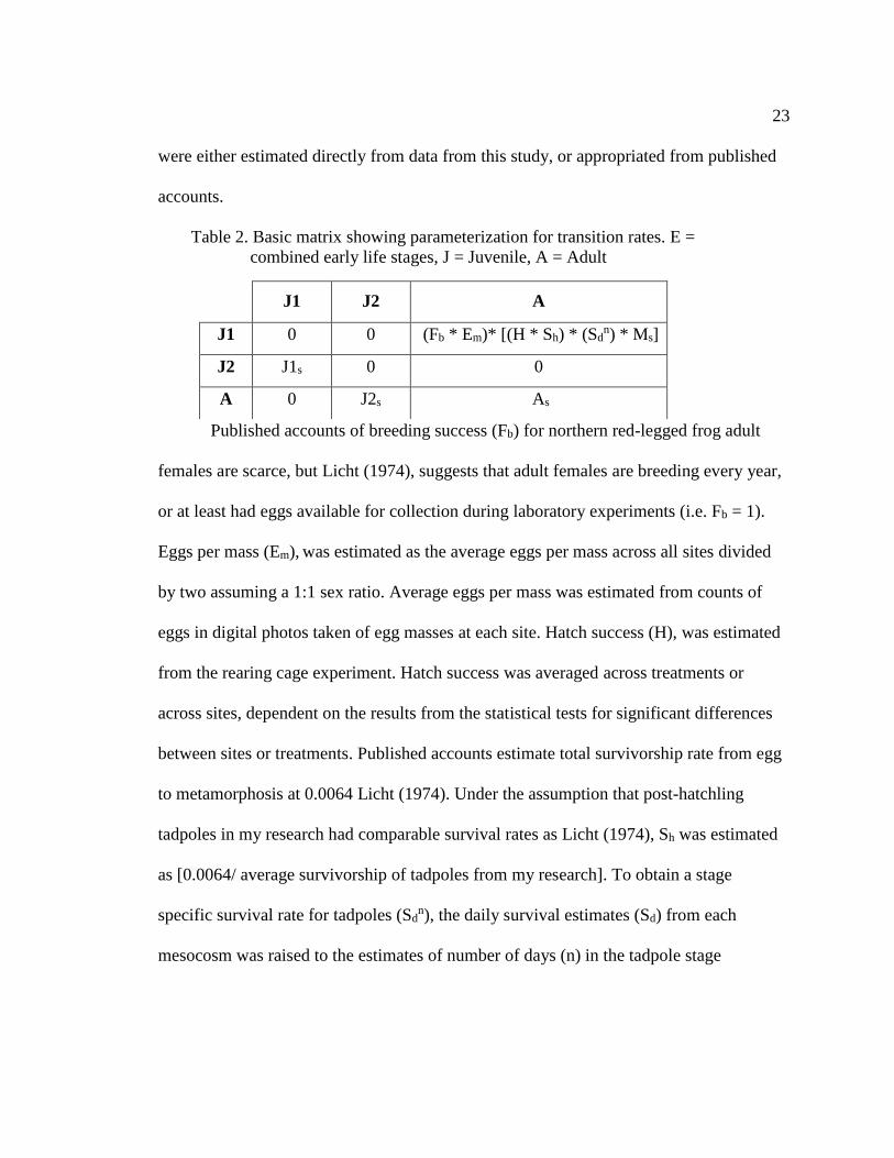
Table 2. Basic matrix showing parameterization for transition rates. E = combined early
life stages, J = Juvenile, A = Adult ................................................................................... 23
Table 3. Average canopy cover (from Jan. to July), across seven field sites in Oregon and
California. Difference is open minus closed averages. Pr (>|t|) = p-value from paired t-
tests evaluating differences in monthly canopy cover between treatments. Each paired t-
test compared seven data points for monthly canopy cover in each mesocosm for each
site. .................................................................................................................................... 25
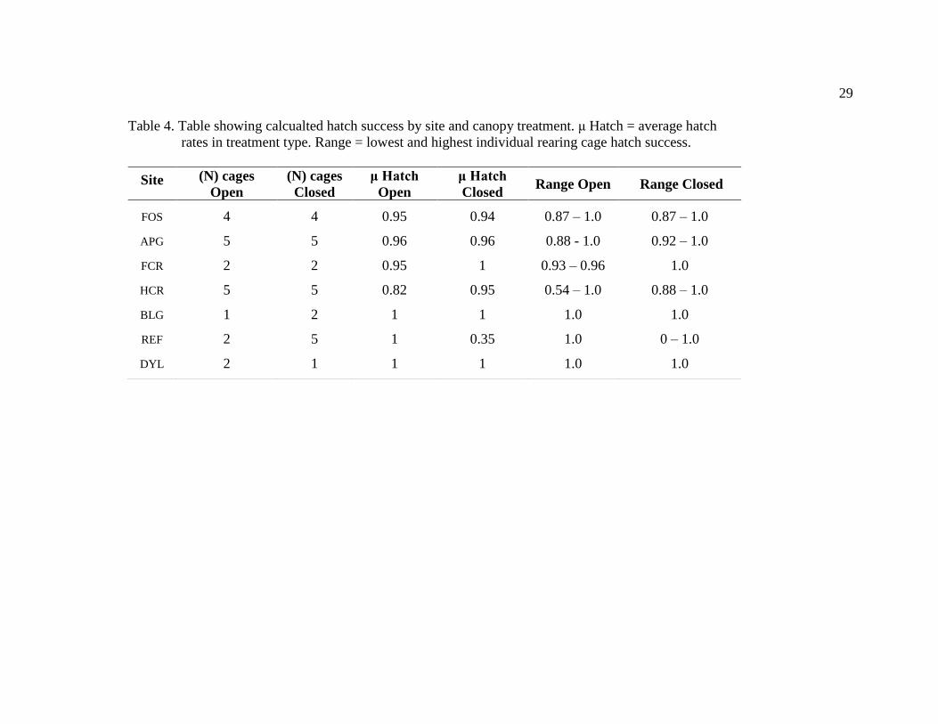
Table 4. Table showing calcualted hatch success by site and canopy treatment. μ Hatch =
average hatch rates in treatment type. Range = lowest and highest individual rearing cage
hatch success. .................................................................................................................... 29
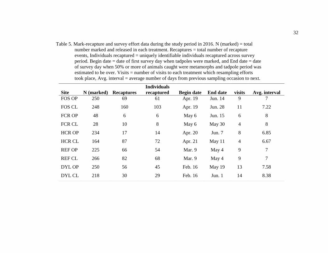
Table 5. Mark-recapture and survey effort data during the study period in 2016. N
(marked) = total number marked and released in each treatment. Recaptures = total
number of recapture events, Individuals recaptured = uniquely identifiable individuals
recaptured across survey period. Begin date = date of first survey day when tadpoles were
marked, and End date = date of survey day when 50% or more of animals caught were
metamorphs and tadpole period was estimated to be over. Visits = number of visits to
each treatment which resampling efforts took place, Avg. interval = average number of
days from previous sampling occasion to next. ................................................................ 32
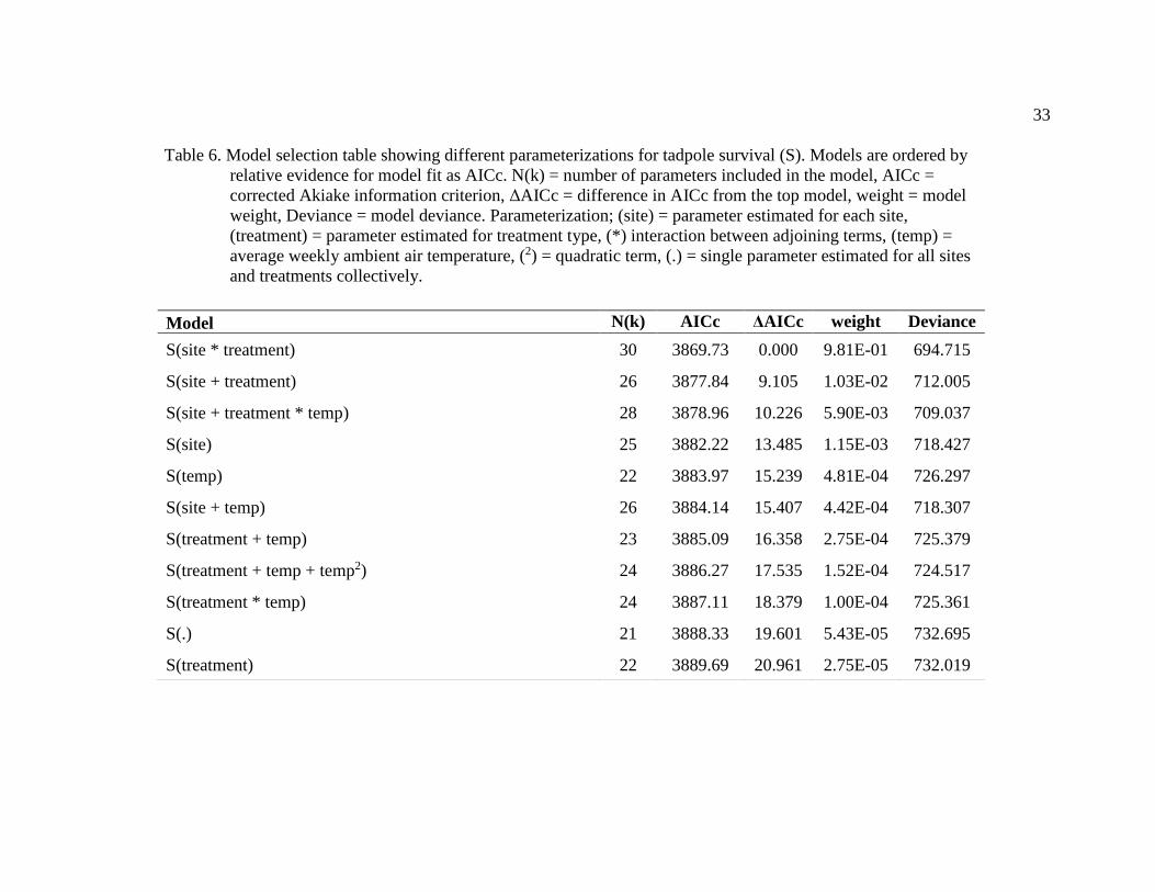
Table 6. Model selection table showing different parameterizations for tadpole survival
(S). Models are ordered by relative evidence for model fit as AICc. N(k) = number of
parameters included in the model, AICc = corrected Akiake information criterion, ΔAICc
= difference in AICc from the top model, weight = model weight, Deviance = model
deviance. Parameterization; (site) = parameter estimated for each site, (treatment) =
parameter estimated for treatment type, (*) interaction between adjoining terms, (temp) =

viii
average weekly ambient air temperature, (2) = quadratic term, (.) = single parameter
estimated for all sites and treatments collectively. ........................................................... 33
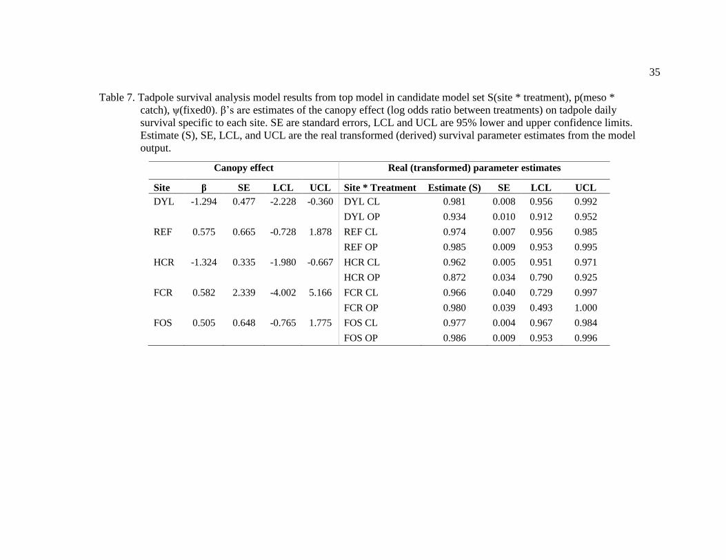
Table 7. Tadpole survival analysis model results from top model in candidate model set
S(site * treatment), p(meso * catch), ψ(fixed0). β’s are estimates of the canopy effect (log
odds ratio between treatments) on tadpole daily survival specific to each site. SE are
standard errors, LCL and UCL are 95% lower and upper confidence limits. Estimate (S),
SE, LCL, and UCL are the real transformed (derived) survival parameter estimates from
the model output. .............................................................................................................. 35
Table 8. Estimates of the average number of days of the tadpole period for each
mesocosm and the overall average between the two treatments. Estimates for HCR and
FCR are taken from open treatments only. ....................................................................... 37
Table 9. Matrix modeling results for stable stage population growth rates (λ). Treatment
= Doyle open, Doyle closed, Hills Creek open, Hills Creek closed. Em = average eggs per
mass from counts across all sites divided in half assuming a 1:1 sex ratio, H = average
egg hatch rate across all treatments and sites, Sh = recruitment into tadpole population
calculated as [0.0064/0.23227], Sd = estimated tadpole daily survival from mark-
recapture analysis, n = tadpole stage length (days). Ms = metamorph survival, Js =
juvenile survival, As = adult survival rates, and Fb = proportion of adult females
reproductively active from Licht (1974). 95% LCL, UCL = lower and upper confidence
limits. ................................................................................................................................ 38
Table 10. Results from the general model evaluated with the early entry dataset. ........... 55
Table 11. Results from the general model evaluated with the late entry dataset. ............. 56

ix
LIST OF FIGURES
Figure 1. Image showing approximate locations of field sites. Outline showing
approximate range of Northern red-legged frogs in Oregon and California, in lighter
color. Three letter acronyms are site names, see Table 1. Image source: Google earth V
7.1.7.2606. (12/13/2015). Image Landsat/Copernicus, Data LDEO-Columbia. ................ 6
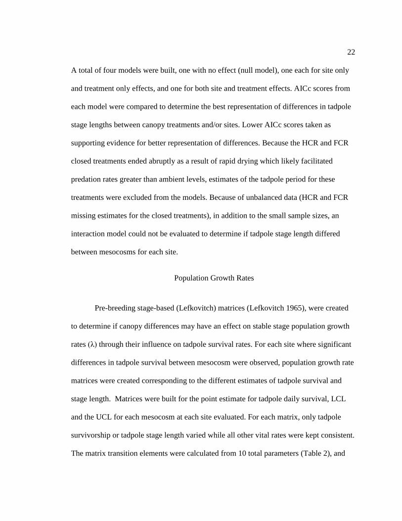
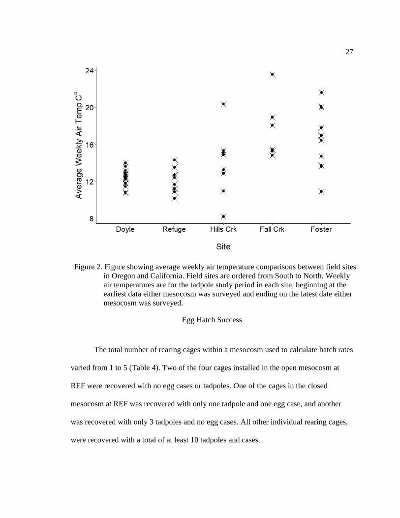
Figure 2. Figure showing average weekly air temperature comparisons between field sites
in Oregon and California. Field sites are ordered from South to North. Weekly air
temperatures are for the tadpole study period in each site, beginning at the earliest data
either mesocosm was surveyed and ending on the latest date either mesocosm was
surveyed. ........................................................................................................................... 27
Figure 3. Tadpole Daily survival estimates from the top performing tadpole survival
model in the candidate model set, S(site * treatment), p(meso * catch), ψ(fixed0). Grey
error bars are lower and upper confidence limits. ............................................................. 34
Figure 4. Projected population growth rates (λ) associated with tadpole survivorship in
open and close mesocosms at sites DYL and HCR. Bar values are λ calculated from the
point estimates of tadpole stage survivorship (Sdn) for each treatment. Error bars are
values for λ calculated from the LCL and UCL of tadpole stage survival for each
treatment. .......................................................................................................................... 39
x
LIST OF APPENDICES
Appendix A: Example of Solar Pathfinder template used to estimate monthly solar
exposure. Above template was used at REF field site in the open mesocosm treatment.
Templates are one-time use and were catalogued by date, location, and treatment type. 53
Appendix B. Model results from the general model evaluated with the early and late entry
datasets (Tables 10 and 11). Survival (S) was estimated for each mesocosm, and
recapture probability was estimated for each mesocosm and fit as a function of total daily
catch. Transition probabilities were fixed to 0. The reported betas (β) are the
untransformed parameter estimates, SE are the standard errors, and LCL and UCL are the
lower and upper confidence limits. Estimates are the real transformed (derived) survival
parameter estimates from the model output. ..................................................................... 55

1
INTRODUCTION
Amphibians are experiencing declines and extinctions at unprecedented rates
(McCallum 2007). Nearly half of all described amphibian species are experiencing some
decline, while one third of described amphibian species are listed as globally threatened
by the International Union for Conservation of Nature (IUCN, Stuart et al. 2004). A
variety of sources contribute to amphibian declines, but availability of suitable habitat
appears to have a significant role in driving population dynamics and species
diversification (Ficetola and De Bernardi 2004, Porej et al. 2004, Cushman 2006). In at
least one study, existing habitat characteristics at the site level appear to be a stronger
determinant of species occurrence than either historic conditions or habitat characteristics
at larger spatial scales (Piha et al. 2007).
One important local habitat characteristic influencing amphibian vital rates is
vegetation in and around the breeding sites (Williams et al. 2008). For example, canopy
cover is negatively associated with somatic growth rates and survival of tadpoles for
several anuran species (Werner and Glennemeier 1999, Thurgate and Pechmann 2007).
Werner and Glennemeier (1999) found American toad (Bufo americanus), wood frog
(Rana sylvatica) and leopard frog (Rana pipiens) tadpoles experienced poorer
survivorship in closed canopy systems compared to open canopy systems.
Thurgate and Pechmann (2007) investigated survivorship differences for tadpoles
of the endangered dusky gopher frog (Rana sevosa) and the relatively common southern
leopard frog (Rana sphenocephala) in closed and open canopy systems. Survivorship to
2
metamorphosis was greater for dusky gopher frogs in open-canopy artificial ponds than
in shaded artificial ponds. The effect of shading was less influential for southern leopard
frogs. The authors suggest the differences in the species’ trajectories between the
endangered dusky gopher frog and the more common southern leopard frog are, at least
in part, due to the different responses to closed canopy breeding sites.
Climate has also been implicated as an influential force on amphibian vital rates
and life history characteristics (Daszak et al. 2005, Pounds et al. 2006, and Todd et al.
2010). Because climate can be influenced by latitude and elevation, amphibian species
that exist across wide latitude and elevation ranges, like northern red-legged frogs (Rana
aurora), also exist across a range of climates. For such species, survival may depend on a
combination of local climates and habitat characteristics. Understanding how a species’
vital rates are related to habitat characteristics in different climates provides managers
and ecologists a tool to evaluate the effects of changes habitat management and climate
change on amphibian population trajectories.
For this thesis work, I evaluated the effect of canopy cover on northern red-legged
frog early stage vital rates, determined whether the effect varied across different climates,
and projected growth rates associated with different tadpole survivorship rates for
populations that demonstrated a clear signal of canopy effects. Specifically I asked four
basic questions: 1) does canopy cover influence egg hatch success and/or tadpole
survival, 2) if canopy cover influences hatch success or tadpole survival, does the effect
change depending on location within species range, 3) if the effect depends on location
with species range, can the differences among canopy treatments be attributed to the

3
different climates at those locations, and 4) does the observed variation in survival
between treatments have a meaningful influence on population growth rates?
Study System
Northern Red-legged frogs are a Ranid species (family Ranidae). The Ranid frog
family is globally distributed, represented on every continent except Antarctica. Species
descriptions and modern genetic based cladistics place nearly 700 species in the family,
representing nearly a quarter of all extant frog species (Scott 2005). Northern red-legged
frog latitudinal distribution extends from the Northern California coast (USA) northward
to coastal British Columbia (Canada). Longitudinal species distribution extends from low
elevations in the Cascade and Sierra Nevada mountain ranges westward to the Pacific
coastline (Stebbins 1951, and Storm 1960). This distribution of populations covers
latitude and elevation gradients, with the potential for different climate and vegetative
conditions. In the United States of America, Northern red-legged frogs are listed as
vulnerable in California (California Department of Fish and Wildlife 2017), sensitive in
Oregon (Oregon Conservation Strategy 2016), and not listed with elevated conservation
status in Washington State. For Northern red-legged frogs, breeding generally begins as
early as October in the southern end of its range in California (personal observation), and
in January to February in Oregon (Storm 1960). The species generally breeds in
permanent and ephemeral pools, and slow moving reaches of streams and rivers.

4
MATERIALS AND METHODS
To determine whether canopy cover has an impact on northern red-legged frog
early life stage vital rates, egg hatch success and tadpole survival data were collected in
open and closed canopy areas at seven breeding sites. Two experimental enclosures (see
below) were created in each field site to create contrasting canopy cover treatments.
Subsamples of eggs were reared and hatched in-situ to estimate hatch success, and mark-
recapture methods were used to estimate tadpole survival. Mark-recapture models
estimating tadpole survival for different site and canopy treatment groupings were
compared to determine if the effect of canopy varied for different populations. Climate
was integrated into mark-recapture models to determine if the differences in tadpole
survival estimates were due to differences in climate. Estimates of vital rates from field
data, along with published accounts, were then used to parameterize population
projection matrices to determine if variation in canopy effects on early stage vital rates
between treatments produced consequential differences in population trajectories.
Field Sites
Field sites were distributed across the southern half of the species latitudinal
range, spanning approximately 560 km from Fort Bragg, California, USA to Sweethome,
Oregon, USA which included sites with a range of different climate conditions (Table 1,
Figure 1). Field sites were selected for accessibility, a mosaic of canopy cover amounts,
and a recent history of breeding activity.

5
Sites included a variety of water body types including seasonal or ephemeral
pools, permanent ponds, and artificial water bodies such as abandoned quarries and
reaches of reservoirs. Land management between the sites included federal agencies and
private industry ownership (Table 1). Sites varied in vegetation abundance and species
composition, as well as hydroperiod and growing season phenology.

6
Figure 1. Image showing approximate locations of field sites. Outline
showing approximate range of Northern red-legged frogs in
Oregon and California, in lighter color. Three letter
acronyms are site names, see Table 1. Image source: Google
earth V 7.1.7.2606. (12/13/2015). Image
Landsat/Copernicus, Data LDEO-Columbia.

7
Table 1. Locations of field sites, listed from North to South. UTMs (Universal Transverse Mercator) are projected in
WGS 84, zone 10. Site abbreviations and description are, FOS = Abandoned quarry adjacent to Foster reservoir;
APG = Slough in the Applegate management unit of Fern Ridge reservoir; FCR = Pond within the Tufti
management unit at Fall Creek reservoir, HCR = Pond located below toe of dam at Hills Creek reservoir, BLG =
Ephemeral pond located within Big Lagoon timber management tract near Orick, CA., REF = Ephemeral
pool/wetland located on Humboldt National Wildlife Refuge, Humboldt County, CA., DYL = Semi-permanent
pond located near Doyle Creek in Fort Bragg, CA. USACE = United States Army Corps of Engineers; GDRC =
Green Diamond Resource Company; USFWS = United States Fish and Wildlife Service, MRC = Mendocino
Redwood Company. Elevation is approximate.
Site General Location UTM Elevation
(m) Water body type
Land
manager/owner
FOS Linn County, Oregon 526000 E 4918614 N 215 Abandoned quarry USACE
APG Lane County, Oregon 472547 E 4878592 N 121 Reservoir USACE
FCR Lane County, Oregon 519330 E 4866634 N 243 Ephemeral pool USACE
HCR Lane County, Oregon 546082 E 4840188 N 384 Pond USACE
BLG Humboldt County, California 413039 E 4551472 N 250 Ephemeral pool GDRC
REF Humboldt County, California 398054 E 4503620 N 3 Seasonally inundated
wetland USFWS
DYL Mendocino County, California 431741 E 435551 N 102 Ephemeral pool MRC

8
Experimental Enclosures
Within each site, two experimental enclosures (hereafter mesocosms) were
created by erecting drift fence material to enclose a section of aquatic area. Mesocosms
were placed to maximize contrast in canopy cover between the treatments. Drift fences
consisted of 122 cm tall woven ground cover material and supported with 122 cm tall
non-painted, non-treated wooden ground stakes. The woven ground cover was a UV
stabilized, permeable polypropylene material, which allowed the transfer of water and
nutrients but restricted tadpoles and hatchlings from passing through.
The bottoms of the drift fences were buried in a shallow trench or secured by
cloth tubes filled with pea gravel (< 2 cm river rock aggregate; hereafter gravel tubes).
The pea gravel was treated with a bleach solution and thoroughly rinsed prior to filling
the gravel tubes to avoid transfer of invasive species or pathogens. Gravel tubes were
approximately 10 cm in diameter and 1.5 m long. Each gravel tube was carefully placed
on top of an approximately 20 cm wide strip of material at the bottom edge of the drift
fence, and overlapped each other by approximately 10 cm.
Mesocosms were constructed to be roughly circular and traverse the aquatic and
terrestrial environments. Within each site, habitat conditions were kept as consistent as
possible between mesocosms. Mesocosms were designed to be similar in size, and to
include shallower (near bank) and deeper parts of the water column. With the exception
of the open canopy mesocosm at FOS, each mesocosm incorporated edges of the water
bodies to allow for recently transformed metamorphs to emigrate from the aquatic

9
environment. At FOS, there were no practical areas to place the open canopy mesocosm
which included pond edges. The open canopy mesocosm at this site was placed in an area
in the middle of the water body that contained a small island of dry land and vegetation
onto which metamorphs could migrate. Similarity between mesocosms was determined
by visual comparisons during initial site visit and time of setup.
Canopy Cover
In order to ensure that mesocosms within each site differed in canopy cover,
canopy cover over each mesocosm was quantified using a Solar Pathfinder™ (The
SolarPathfinder Company, Linden, Tennessee, United States of America). The Solar
Pathfinder™ device estimates the percent of solar light reaching the point of
measurement. This is accomplished by tracing the reflection on a semi-transparent
polycarbonate dome of obstructions overhead and on the horizon onto a template sheet
underneath the dome (Appendix A). Canopy cover is then estimated as the difference
between the amount of light reaching the site and total possible under unobstructed
conditions (100%). Using the Solar Pathfinder™ device, measurements of canopy cover
were taken only once during any time of the year and estimates of monthly canopy cover
were calculated from the template sheet (Appendix A). Paired t-tests were performed for
each site (a total of six different t-tests) to determine if monthly canopy cover was
different between treatments during the survey period (January through July).
Temperature Data

10
Mean weekly air temperature was used as an index of climate differences between
sites. Air temperature was chosen to represent climate in this study because it can be
easily retrieved from historical records or collected on site with little effort for managers.
Air temperature can also be measured on fine spatial scales without specialized
equipment, and is directly relatable to potential effects of climate change at the breeding
site level.
Temperature data were recorded using HOBO® UA-001-08 eight kilobyte data
loggers (Onset Computer Corporation®; Bourne, Massachusetts, United States of
America). A single data logger was placed in a location within each site, approximately
halfway between the mesocosms, and suspended from emergent or bankside vegetation to
record ambient air temperature. Each data logger was set to take temperature
measurements once per hour. Temperature data from HOBO data loggers were collected
at least once during the field season for each site, and when the study period was
completed. After temperature data were verified and corrected, hourly temperature
readings were averaged over a 24 hour period beginning 12 am (00:00 hours) and ending
at 11 pm (23:00 hours) the same calendar day. Daily averages were then used to calculate
mean weekly temperatures over seven day periods, corresponding to each date of site
visit plus the 6 days prior to each site visit.
Differences in mean weekly air temperatures between sites were evaluated with a
Tukey-Honestly Significant Difference (TukeyHSD) test for multiple comparisons on a
fitted analysis of variance (ANOVA) general linear model. All statistical analyses for

11
temperature, and for each following section, were done using the R statistical software
program (R core team 2017).
Temperature Data Corrections
Some temperatures from the data loggers recording air temperature were
unavailable or corrupted. Data sets with suspect or missing air temperatures from
dataloggers were plotted against PRISM climate datasets (PRISM Climate Group,
Oregon State University), to check for consistencies between the two data sets for periods
just prior to and after the missing data points from the dataloggers. PRISM datasets and
datalogger data sets were also compared to check for divergence between the two
datasets for the suspect data from the dataloggers. The PRISM climate datasets used for
comparisons corresponded to the beginning and ending times of the datalogger sets and
had a 4 km scale resolution. Missing air temperature data and data determined to be
inaccurate were replaced with data from the PRISM climate datasets specific to each site.
Egg Hatch Success
To estimate egg hatching success, eggs from 2-5 sample egg masses per site were
caged within individual mesh-fabric enclosures (hereafter rearing cages). A subsample of
25 eggs from each egg mass was placed in a rearing cage in each of the two experimental
mesocosms. Rearing cages were built from untreated, unpainted wooden frames covered
with tulle fabric. Rearing cages measured approximately 45 cm width x 45 cm length x
90 cm height. The tops of the rearing cages were left open to facilitate observations of
egg development. Rearing cages were placed next to each other in a row within each

12
mesocosm, and secured with wooden ground stakes. Rows of rearing cages within a site
were oriented in the same direction. The position within rows of egg samples from the
same egg mass was randomized to account for possible effects of being in an exterior
versus interior rearing cage.
Rearing cages were checked once every seven to ten days to determine numbers
of hatched and unhatched eggs, development stages of unhatched eggs, and numbers of
non-viable embryos. During each check, rearing cages were removed from their anchors
and slowly lifted to water surface until eggs, tadpoles or egg cases were visible. If there
were unhatched eggs during a check, the rearing cage was placed back into its original
position and unhatched eggs were allowed to develop further. During intermediate and
final cage checks, some cages had holes in the mesh fabric and repairs were made as
necessary.
The total number of eggs present immediately prior to hatching was often less
than the 25 originally placed in the rearing cages. Because the fate of these eggs was
unknown, hatch success was calculated as the proportion of hatched eggs to the total
available to hatch, rather than the original number of 25 eggs. The number of hatched
eggs used in the calculation was the highest total count either of tadpoles present, or of
empty egg cases (assumed to be the remaining vitelline membrane). Total available to
hatch was calculated as the sum of the number of hatched eggs plus the number of
unhatched non-viable eggs. Mesocosm and site specific mean hatch success was
determined as a weighted average (i.e. mesocosm or site specific sum of hatched eggs
divided by sum of total available to hatch).

13
Nonparametric analyses were used because variances could not be estimated for
some mesocosms or sites, and because some mesocosms and sites had very small samples
sizes. Variances were not able to be estimated for some treatment and sites because some
mesocosms had only one rearing cage that produced hatch success data, some mesocosms
had the exact same hatch success for all the rearing cages, and some sites had fewer than
4 total rearing cages. Mesocosm and site effects on ranks of egg hatch success were fit
with an ordered logistic regression model using the R package MASS (Venables and
Ripley 2002). Significance of overall treatment and site effects were determined from
type 2 ANOVA sum of squares reductions using the R package car (Fox and Weisberg
2011).
Tadpole Mark-Recapture
Mark-recapture data were collected throughout the tadpole development period at
five of the previously identified seven field sites. Excessive growth of reed canary grass
(Phalaris arundinacea) at APG resulted in no tadpole captures, and dense submerged
woody debris at BLG limited tadpole captures to only two animals, and thus these two
sites were excluded from the tadpole survival analysis.
Sample populations of tadpoles for mark-recapture came from tadpoles hatched
from naturally-occurring and seeded egg masses in each mesocosm. Seeding egg masses
into mesocosms was accomplished by cutting the vegetation that egg masses were
attached to and transferring them using a five gallon bucket filled with water. After
transferring, the vegetation attached to the egg mass was secured to a bamboo stake.
14
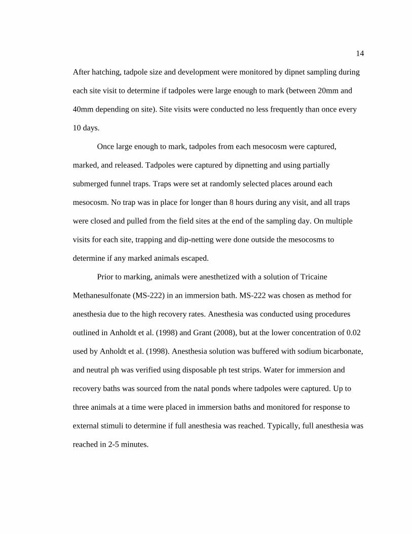
After hatching, tadpole size and development were monitored by dipnet sampling during
each site visit to determine if tadpoles were large enough to mark (between 20mm and
40mm depending on site). Site visits were conducted no less frequently than once every
10 days.
Once large enough to mark, tadpoles from each mesocosm were captured,
marked, and released. Tadpoles were captured by dipnetting and using partially
submerged funnel traps. Traps were set at randomly selected places around each
mesocosm. No trap was in place for longer than 8 hours during any visit, and all traps
were closed and pulled from the field sites at the end of the sampling day. On multiple
visits for each site, trapping and dip-netting were done outside the mesocosms to
determine if any marked animals escaped.
Prior to marking, animals were anesthetized with a solution of Tricaine
Methanesulfonate (MS-222) in an immersion bath. MS-222 was chosen as method for
anesthesia due to the high recovery rates. Anesthesia was conducted using procedures
outlined in Anholdt et al. (1998) and Grant (2008), but at the lower concentration of 0.02
used by Anholdt et al. (1998). Anesthesia solution was buffered with sodium bicarbonate,
and neutral ph was verified using disposable ph test strips. Water for immersion and
recovery baths was sourced from the natal ponds where tadpoles were captured. Up to
three animals at a time were placed in immersion baths and monitored for response to
external stimuli to determine if full anesthesia was reached. Typically, full anesthesia was
reached in 2-5 minutes.
15
Once under anesthesia, tadpoles were marked with Visible Implant Elastomer
(VIE) tags, (Northwest Marine Technologies Inc., Shaw Island, Washington, USA). Each
animal was marked with a four-tag color coded sequence, with two tags on either side of
the tail. Tags were injected between the epidermis and muscle tissues using a 0.3 cc
insulin syringe with a 29 gauge needle. One pair of tags was placed on the dorsal side and
the other pair on the ventral side of the tail. Each pair of tags was adjacent to each other
and located near where tail muscle telomeres meet the fins.
After marking, tadpoles were placed in the recovery bath and monitored for
recovery. Full recovery was then determined by monitoring tadpoles in holding
containers, watching for active swimming and burst swimming when gently prodded.
Tadpoles that had fully recovered were released into the same mesocosms from which
they were captured. Water for recovery baths, pre and post-marking holding containers
were refreshed between batches of tadpoles.
Methods for animal manipulation including anesthesia and recovery, capture,
marking and confinement to mesocosms followed those approved in my Institutional
Animal Care and Use Committee (IACUC) protocol (number 15/16.W.59-A).
Tadpole Data Collection
For field sites FOS, FCR, HCR, REF, and DYL there were at least four sampling
occasions for both mesocosm treatments. Resampling in the closed mesocosm at HCR
ended when water levels in the pond dropped suddenly between the third and fourth site
visits, and all tadpoles disappeared. These disappearances could have been caused by
tadpoles escaping through an undetected hole in the mesocosm or a mass predation event

16
precipitated by the receding water. Raccoons (Procyon lotor) patrol the banks regularly,
and large wading birds like Great blue heron (Ardea herodias) are commonly observed in
the field site. The FCR closed treatment ended after the fourth sampling occasion when
water levels dropped rapidly in this mesocosm between the fourth and fifth sampling
occasion and all the animals vanished abruptly. The apparent extirpation of this sample
population could have been caused by a rapid metamorphosis following the dropping
water levels. A more plausible explanation is that low water levels facilitated high
predation rates by juvenile and adult bullfrogs (Lithobates catesbeianus), which were
commonly observed within the mesocosm. There was no detectable hole in the drift
fence.
Tadpole Data Analysis
Two important sources of variation in tadpole vital rates which influence
recruitment into the metamorph life-stage are: 1) daily survival rates, and 2) the overall
length of time of the tadpole stage. Survival and stage length were estimated separately.
Mark-Recapture Analysis
Daily survival rates were estimated using the RMark package (Laake 2013) in R.
Multistate models were used to evaluate these data because each mesocosm represents a
unique grouping of animals analogous to the different states of animals in the multistate
model framework (Arnason 1973, Schwarz et al. 1993). Recapture probabilities were
constrained to zero for survey days on which sites were not visited.
17
Although a few (14 of 583 total recaptures) animals were recaptured outside of
the original mesocosms they were released in, no animals were recaptured inside a
different mesocosm than the one of original release. Because the proportion of animals
recaptured outside their original mesocosm was extremely low, and those tadpoles were
captured near their original mesocosm, dispersal among mesocosms could be effectively
represented as 0.
During model fitting, two candidate model sets were created. The first model set
was created to determine the most appropriate representation of recapture probability (p).
Assuming that survival varied independently among all mesocosms, recapture probability
was evaluated as 1) a single estimate across all mesocosms and sites, 2) different
estimates for each site with a single estimate for both mesocosm treatments within a site,
3) no site differences but different estimates for mesocosm treatments (open or closed
canopy) within sites, 4) additive site and treatment effects, and 5) different estimates for
each site with different effects of treatment type for each site. For each of these
parameterizations, p was assumed to be either 1) the same across all sampling occasions,
or 2) a function of total animals captured in a survey day for each mesocosm, reflecting
the effort spent capturing during each visit.
Once the best fitting parameterization for p was determined, only that model
structure for p was used when fitting different models of daily survival rates (S). To
determine if tadpole survivorship was influenced by the canopy cover treatment, a second
candidate model set was built and evaluated. This model set contained parameterizations
of S as 1) a single estimate across all mesocosms and sites, 2) different estimates for each

18
site but with a single estimate for both mesocosm treatments within a site, 3) no site
differences but different estimates for mesocosm treatments (open or closed canopy)
within sites, 4) additive site and treatment effects, and 5) different estimates for each site
with different effects of treatment type for each site. Climate was also fit to models with
different parameterizations of S, as a linear function of mean weekly air temperature to
determine if there was a treatment by temperature interaction. Nonsense estimates (e.g. S
= 1 or 0), and inflated standard errors tend to occur when attempting to estimate
parameters with relatively sparse data, in particular for models with large numbers of
parameters (k). Because of this, a time dependent model where S varied between
sampling occasions is not included in the reported final candidate model set for S.
At some point, tadpoles transformed into metamorphs and emigrated from the
pond. Because tadpoles were marked on the tail, which is lost to reabsorption during the
transformation process, the tags were unrecoverable even if the animal is recaptured. To
account for the apparent loss of animals due to transformation, instead of actual loss due
to mortality, the mark-recapture dataset for each mesocosm was truncated when at least
half of the animals caught in a survey day were considered metamorphs (> Gosner stage
42-43, Gosner 1960). While this method does not account for all the uncertainty between
apparent and actual mortality, the timing when at least half the animals caught in a day
were metamorphs was interpreted as the first indication that the population has
transitioned from mostly tadpoles to mostly metamorphs. For each of the sites this
transition happened relatively shortly after the first metamorph was detected, usually
within one to two weeks.

19
Models within each candidate model set were assessed for relative support using
Akiake information criterion corrected for small sample size (AICc) (Akiake 1973,
Burnham and Anderson 2002), and by model weight. Comparison among candidate
models using AICc assumes that data are not overdispersed, where overdispersion is
represented as c values (Burnham and Anderson 2002). Overdispersion was checked for
using a bootstrap simulation. The bootstrap simulation was completed by recreating
multiple alternate datasets in R, with the mark-recapture parameters (e.g. timing of entry
into the marked populations, recapture probability, and survival probability) informed by
estimates from the general model evaluated with the field data. The bootstrap resampling
and evaluation process was completed 100 times. If results from the bootstrap simulation
suggest overdispersion is prevalent (i.e. average c values from the bootstrap simulation
are greater than the observed c value form the original data set), final AICc values can be
adjusted to Quasi AICc (QAICc) to account for the overdispersion (Burnham and
Anderson 2002). If the average c value from the bootstrap simulation is smaller than the
observed c from the original data, AICc values are not adjusted.
Once the top-performing model was selected and if it contained a site effect,
treatment effect, or combination of both, 95% lower and upper confidence limits (LCLs
and UCLs) were used as a measure of significance. Comparison of the LCLs and UCLs
on the transformed parameters (survival estimates) for pairs of sites, or pairs of
treatments within a site, and whether the LCLs and UCLs for the estimated canopy
effects (log odds ratios) encompassed zero were used to determine if there was a clear
signal of a treatment effect. If the range of confidence limits between the estimates did
20
not show any overlap, and if the confidence limits on the estimated canopy effects did not
encompass zero, this was interpreted as compelling evidence for a treatment effect.
Estimated canopy effects for each site were calculated by combining the estimates for the
average treatment effect and the site specific treatment effect of the untransformed betas.
Standard errors for the site-specific estimated canopy treatment effects were calculated
using the delta method in Rmark package (Laake 2013).
Tadpole Tag Loss
Although infrequent, some tag loss was observed during recapture occasions. For
tadpoles with complete sequences but partially lost individual tags (i.e. some of the
elastomer tag was still visible), the individual tags were reinjected. If an individual tag
was completely lost, the remaining tag colors and their position within the original
sequence were recorded.
Partial color sequences in the field were cross-checked against the known color
sequences used for each mesocosm, and animals with missing tags were matched with a
short list of possible animals. In some cases, it was possible to reduce the list to a single
individual animal based on when combinations were used, recaptures of other tadpoles
with similar combinations, tadpole development, and which mesocosm animals were
released in because there was effectively no dispersal between mesocosms. Multiple
recaptures of tadpoles with the same partial combination, although rare (19 of 583 total
recaptures) were assumed to be the same animal. In most cases partial combinations
could be assigned to multiple possible marked individuals. If all possible matches were
originally marked on the same date, the unidentified animal was assigned to one of the
21
possible matches at random. If at least one of the possible matches was originally marked
on a different date, the unidentified animal was assigned an identification corresponding
with the earliest possible, or the latest possible entry date into the marked population
(early and late datasets). It was assumed no animals completely lost all four tags.
The general model for the mark-recapture tadpole survival analysis was evaluated
using both the early and late entry datasets to look for differences in survival estimates. In
the event that both data sets returned estimates without substantial differences for every
survival parameter (i.e. differences between analogous tadpole survival estimates, less
than one standard error apart, measured using the smaller of the two comparable standard
errors), then either dataset could be used and the choice to use one over the other would
be arbitrary. If however, at least one set of analogous survival parameters were greater
than one standard error apart, the choice of the data set to use was based on which
produced estimates with the smaller of the standard errors on the untransformed betas (β).
The remainder of the survival analysis was done using the chosen data set. Results from
the global model used in dataset selection evaluated with the early and late entry datasets
are reported in Appendix B.
Tadpole Stage Length
Tadpole stage length for each mesocosm was estimated as the length of time from
when the tadpole sampling started to the first sampling occasion when more than half of
the animals caught (marked or unmarked) were metamorphs. A set of generalized linear
models were compared to determine if tadpole stage length varied between treatments or
sites. For each model the response variable was the estimate of the tadpole stage length.
22
A total of four models were built, one with no effect (null model), one each for site only
and treatment only effects, and one for both site and treatment effects. AICc scores from
each model were compared to determine the best representation of differences in tadpole
stage lengths between canopy treatments and/or sites. Lower AICc scores taken as
supporting evidence for better representation of differences. Because the HCR and FCR
closed treatments ended abruptly as a result of rapid drying which likely facilitated
predation rates greater than ambient levels, estimates of the tadpole period for these
treatments were excluded from the models. Because of unbalanced data (HCR and FCR
missing estimates for the closed treatments), in addition to the small sample sizes, an
interaction model could not be evaluated to determine if tadpole stage length differed
between mesocosms for each site.
Population Growth Rates
Pre-breeding stage-based (Lefkovitch) matrices (Lefkovitch 1965), were created
to determine if canopy differences may have an effect on stable stage population growth
rates (λ) through their influence on tadpole survival rates. For each site where significant
differences in tadpole survival between mesocosm were observed, population growth rate
matrices were created corresponding to the different estimates of tadpole survival and
stage length. Matrices were built for the point estimate for tadpole daily survival, LCL
and the UCL for each mesocosm at each site evaluated. For each matrix, only tadpole
survivorship or tadpole stage length varied while all other vital rates were kept consistent.
The matrix transition elements were calculated from 10 total parameters (Table 2), and
23
were either estimated directly from data from this study, or appropriated from published
accounts.
Table 2. Basic matrix showing parameterization for transition rates. E =
combined early life stages, J = Juvenile, A = Adult
Published accounts of breeding success (Fb) for northern red-legged frog adult
females are scarce, but Licht (1974), suggests that adult females are breeding every year,
or at least had eggs available for collection during laboratory experiments (i.e. Fb = 1).
Eggs per mass (Em), was estimated as the average eggs per mass across all sites divided
by two assuming a 1:1 sex ratio. Average eggs per mass was estimated from counts of
eggs in digital photos taken of egg masses at each site. Hatch success (H), was estimated
from the rearing cage experiment. Hatch success was averaged across treatments or
across sites, dependent on the results from the statistical tests for significant differences
between sites or treatments. Published accounts estimate total survivorship rate from egg
to metamorphosis at 0.0064 Licht (1974). Under the assumption that post-hatchling
tadpoles in my research had comparable survival rates as Licht (1974), Sh was estimated
as [0.0064/ average survivorship of tadpoles from my research]. To obtain a stage
specific survival rate for tadpoles (Sdn), the daily survival estimates (Sd) from each
mesocosm was raised to the estimates of number of days (n) in the tadpole stage
J1 J2 A
J1 0 0 (Fb * Em)* [(H * Sh) * (Sdn) * Ms]
J2 J1s 0 0
A 0 J2s As

24
estimated for each breeding site. Metamorph survival (Ms) values were taken from Licht
(1974).
In his research, Licht (1974) estimated a combined adult and juvenile survival
rate, as well as an adult only survival rate. However, there is not enough information in
that study to determine juvenile only survival with high confidence. Assuming that
juvenile survival is likely more similar to that of adults than metamorphs due to their
shared behavioral traits (e.g. emigration from natal ponds and overwintering dormant
cycles), a single value was used for both Js and As. Because juveniles are not
reproductively active in their first year (Licht 1974), the matrix includes a transition rate
from first year juvenile (J1s) to second year juvenile (J2s). The matrices evaluated here
also assume second year juveniles are not reproductively active. All survivorship rates
were assumed to be similar between sexes.
To determine the relative contribution of the early stages to population growth, an
elasticity analysis was done (Caswell 2000). Elasticities were calculated analytically
using eigenvalues and eigenvectors (de Kroon et al. 1986), in the R software program.
Elasticities were evaluated using a matrix with the mean value of for the early stage
survival rates for the mesocosms included in individual matrices used in the analysis
above.

25
RESULTS
Canopy Cover
Canopy cover was different between treatments for most sites during the survey
period from January through July (Table 3). The greatest observed difference in mean
canopy cover between treatments for the study period was for HCR at 54.07 %, while the
smallest difference was for BLG at 9.93 % (Table 3).
Table 3. Average canopy cover (from Jan. to July), across seven field sites in
Oregon and California. Difference is open minus closed averages. Pr
(>|t|) = p-value from paired t-tests evaluating differences in monthly
canopy cover between treatments. Each paired t-test compared seven data
points for monthly canopy cover in each mesocosm for each site.
Site
Avg. open
(se)
Avg. closed
(se) Difference Pr (>|t|)
FOS 28.78 (5.11) 56.71 (7.75) 27.93 0.0127
APG 31.89 (12.97) 62.71 (11.28) 30.82 0.0987
FCR 10.50 (4.34) 59.07 (11.70) 48.57 0.0051
HCR 7.50 (2.69) 61.57 (2.81) 54.07 < 0.0001
BLG 89.78 (4.61) 99.71 (0.18) 9.93 0.0748
REF 7.00 (1.63) 36.35 (3.17) 29.35 < 0.0001
DYL 12.50 (1.17) 60.21 (11.59) 47.71 0.0061

26
Temperature
Because sites DYL, REF, HCR, FCR, and FOS were they only ones to yield both
egg hatch success and tadpole survival data, they were the only sites included in the
temperature analysis. The average of the daily mean air temperatures during tadpole
study periods was highest for FCR at 17.313 C°, and lowest for REF at 12.106 C°, with
DYL, HCR and FOS at 12.313 C°, 13.868 C°, and 16.612 C° respectively. Results from
the TukeyHSD multiple comparisons test on differences in range of temperatures
between sites suggested significant differences in mean weekly air temperature between
DYL with FCR and FOS (adjusted P = <0.0001 and 0.001), but not REF or HCR
(adjusted P = 0.999 and 0.645); significant differences between REF with FCR and FOS
(adjusted P = 0.001 and 0.003) but not HCR (adjusted P = 0.641), marginal differences
between HCR with FCR (adjusted P = 0.06) but none with FOS (adjusted P = 0.159), and
no difference between FCR with FOS (adjusted P= 0.923), (Figure 2).
27
Egg Hatch Success
The total number of rearing cages within a mesocosm used to calculate hatch rates
varied from 1 to 5 (Table 4). Two of the four cages installed in the open mesocosm at
REF were recovered with no egg cases or tadpoles. One of the cages in the closed
mesocosm at REF was recovered with only one tadpole and one egg case, and another
was recovered with only 3 tadpoles and no egg cases. All other individual rearing cages,
were recovered with a total of at least 10 tadpoles and cases.
Figure 2. Figure showing average weekly air temperature comparisons between field sites
in Oregon and California. Field sites are ordered from South to North. Weekly
air temperatures are for the tadpole study period in each site, beginning at the
earliest data either mesocosm was surveyed and ending on the latest date either
mesocosm was surveyed.

28
Average hatch success was greater than 80% in all mesocosms except for the
closed treatment at REF. There was not a significant difference in hatch success between
canopy treatments across sites (χ2 = 0.247, df = 1, P = 0.619). No differences in hatch
success were observed between sites (χ2 = 9.188, df = 6, P = 0.163).
29
Table 4. Table showing calcualted hatch success by site and canopy treatment. μ Hatch = average hatch
rates in treatment type. Range = lowest and highest individual rearing cage hatch success.
Site (N) cages
Open
(N) cages
Closed
μ Hatch
Open
μ Hatch
Closed Range Open Range Closed
FOS 4 4 0.95 0.94 0.87 – 1.0 0.87 – 1.0
APG 5 5 0.96 0.96 0.88 - 1.0 0.92 – 1.0
FCR 2 2 0.95 1 0.93 – 0.96 1.0
HCR 5 5 0.82 0.95 0.54 – 1.0 0.88 – 1.0
BLG 1 2 1 1 1.0 1.0
REF 2 5 1 0.35 1.0 0 – 1.0
DYL 2 1 1 1 1.0 1.0

30
Tadpole Mark-Recapture
A total of 1931 tadpoles were captured, marked and released across five field
sites. Total length of time for surveys varied from 20 days in the HCR open treatment to
106 days in the DYL closed treatment. Average number of days from previous sampling
occasion to next varied from 6.67 days in HCR closed treatment to 8.38 days in the DYL
closed treatment (Table 5).
The late entry dataset was selected to complete the survival analysis because daily
survival could not be estimated for all the mesocosms under the general model using the
early entry dataset. In addition to the inability to estimate survival for all mesocosms, for
the mesocosms in which survival was estimated, the uncertainty associated with the
untransformed parameters was greater for the early entry dataset compared to the late
entry dataset. Although the late entry dataset was chosen to complete the tadpole survival
analysis, the top model from the late entry dataset model selection table was evaluated
with early entry dataset. Those results did not qualitatively differ from the conclusions of
the tadpole survival analysis using the late entry dataset. The results reported below are
based on the late entry dataset.
The overdispersion (c) value from the model run with the original data was 3.637.
The bootstrap simulation was run 100 times and returned a mean c = 7.203, which gives a
derived c = 0.504. The derived c and the scaling factor was rounded up to one, and the
model selection table did not change.

31
The top performing recapture probability model estimated p for each mesocosm
treatment, and as a function of daily number of animals caught in each treatment. This
model carried 100 percent model weight and had an AICc score > 100 points lower than
the next best fitting model. Among the suite of models evaluated for tadpole survival, the
model that included a treatment by site interaction had the lowest AICc score and carried
98.1% model weight (Table 6). The next best fitting model included both site and
treatment as factors, but without an interaction between the two variables. There was no
evidence for a linear or quadratic relationship between air temperature and tadpole
survival.
The highest estimated daily survival from the top model was for the FOS open
treatment at 0.9857 (SE = 0.0087, CI = 0.9533, 0.9957). The lowest estimated daily
survival was for the HCR open treatment at 0.8717 (SE = 0.0337, CI = 0.7898, 0.9247)
(Figure 3). The lower and upper confidence limits between treatments overlapped for
FOS, FCR and REF, whereas for DYL and HCR the limits show a clearer separation
between treatments.
32
Table 5. Mark-recapture and survey effort data during the study period in 2016. N (marked) = total
number marked and released in each treatment. Recaptures = total number of recapture
events, Individuals recaptured = uniquely identifiable individuals recaptured across survey
period. Begin date = date of first survey day when tadpoles were marked, and End date = date
of survey day when 50% or more of animals caught were metamorphs and tadpole period was
estimated to be over. Visits = number of visits to each treatment which resampling efforts
took place, Avg. interval = average number of days from previous sampling occasion to next.
Site N (marked) Recaptures
Individuals
recaptured Begin date End date visits Avg. interval
FOS OP 250 69 61 Apr. 19 Jun. 14 9 7
FOS CL 248 160 103 Apr. 19 Jun. 28 11 7.22
FCR OP 48 6 6 May 6 Jun. 15 6 8
FCR CL 28 10 8 May 6 May 30 4 8
HCR OP 234 17 14 Apr. 20 Jun. 7 8 6.85
HCR CL 164 87 72 Apr. 21 May 11 4 6.67
REF OP 225 66 54 Mar. 9 May 4 9 7
REF CL 266 82 68 Mar. 9 May 4 9 7
DYL OP 250 56 45 Feb. 16 May 19 13 7.58
DYL CL 218 30 29 Feb. 16 Jun. 1 14 8.38
33
Table 6. Model selection table showing different parameterizations for tadpole survival (S). Models are ordered by
relative evidence for model fit as AICc. N(k) = number of parameters included in the model, AICc =
corrected Akiake information criterion, ΔAICc = difference in AICc from the top model, weight = model
weight, Deviance = model deviance. Parameterization; (site) = parameter estimated for each site,
(treatment) = parameter estimated for treatment type, (*) interaction between adjoining terms, (temp) =
average weekly ambient air temperature, (2) = quadratic term, (.) = single parameter estimated for all sites
and treatments collectively.
Model N(k) AICc ΔAICc weight Deviance
S(site * treatment) 30 3869.73 0.000 9.81E-01 694.715
S(site + treatment) 26 3877.84 9.105 1.03E-02 712.005
S(site + treatment * temp) 28 3878.96 10.226 5.90E-03 709.037
S(site) 25 3882.22 13.485 1.15E-03 718.427
S(temp) 22 3883.97 15.239 4.81E-04 726.297
S(site + temp) 26 3884.14 15.407 4.42E-04 718.307
S(treatment + temp) 23 3885.09 16.358 2.75E-04 725.379
S(treatment + temp + temp2) 24 3886.27 17.535 1.52E-04 724.517
S(treatment * temp) 24 3887.11 18.379 1.00E-04 725.361
S(.) 21 3888.33 19.601 5.43E-05 732.695
S(treatment) 22 3889.69 20.961 2.75E-05 732.019

34
Figure 3. Tadpole Daily survival estimates from the top performing tadpole survival model in the
candidate model set, S(site * treatment), p(meso * catch), ψ(fixed0). Grey error bars are
lower and upper confidence limits.
35
Table 7. Tadpole survival analysis model results from top model in candidate model set S(site * treatment), p(meso *
catch), ψ(fixed0). β’s are estimates of the canopy effect (log odds ratio between treatments) on tadpole daily
survival specific to each site. SE are standard errors, LCL and UCL are 95% lower and upper confidence limits.
Estimate (S), SE, LCL, and UCL are the real transformed (derived) survival parameter estimates from the model
output.
Canopy effect Real (transformed) parameter estimates
Site β SE LCL UCL Site * Treatment Estimate (S) SE LCL UCL
DYL -1.294 0.477 -2.228 -0.360 DYL CL 0.981 0.008 0.956 0.992
DYL OP 0.934 0.010 0.912 0.952
REF 0.575 0.665 -0.728 1.878 REF CL 0.974 0.007 0.956 0.985
REF OP 0.985 0.009 0.953 0.995
HCR -1.324 0.335 -1.980 -0.667 HCR CL 0.962 0.005 0.951 0.971
HCR OP 0.872 0.034 0.790 0.925
FCR 0.582 2.339 -4.002 5.166 FCR CL 0.966 0.040 0.729 0.997
FCR OP 0.980 0.039 0.493 1.000
FOS 0.505 0.648 -0.765 1.775 FOS CL 0.977 0.004 0.967 0.984
FOS OP 0.986 0.009 0.953 0.996

36
Tadpole Stage Length
The observed tadpole stage length in the sites which had estimates for both
mesocosms was not consistent. For one site the open treatment had a longer stage length,
one site had a longer stage in the closed treatment, and the stages were the same length in
another site (Table 8). There was no estimate for the closed canopy treatments at HCR
and FCR so the open treatment estimate was taken to be the site estimate.
The top performing model for tadpole stage length suggested tadpole period
varied with site only, though the model where tadpole period varied with site and canopy
treatment (additive model) was very similar (ΔAIC = 0.33). The no effect model, and the
canopy treatment only effect model performed worse (ΔAIC = 42.205 and 34.354
respectively). Although the site only model and the additive model had approximately
equivalent AIC scores, the site only model was chosen because stage length did not
appear to differ significantly with treatment in the additive model (z = -1.291, P = 0.197).
Because there was little support that stage length differed between treatments, the
estimates of tadpole period for each site were averaged across canopy treatments to
obtain site estimates.

37
Table 8. Estimates of the average number of
days of the tadpole period for each
mesocosm and the overall average
between the two treatments. Estimates
for HCR and FCR are taken from open
treatments only.
Site Open Closed Average days
DYL 106 93 99.5
REF 56 56 56
HCR 48 - 48
FCR 40 - 40
FOS 56 70 63
Population Growth Rates
Because tadpole survival estimates differed between canopy cover treatment only
at HCR and DYL, these sites were the only ones used in the matrix analysis. At both
sites, the difference in 𝜆 associated with tadpole survivorship between treatments
corresponded to a 30% yearly decline for the open treatments, and a stable or nearly
stable population growth for the closed treatments (Table 9, Figure 4). The elasticity
analysis indicated that population growth rates are most sensitive to changes in adult
survival with an elasticity value of 0.554, and less sensitive to changes in the combined
early stages survival with an elasticity value of 0.148.

38
Table 9. Matrix modeling results for stable stage population growth rates (λ). Treatment = Doyle open, Doyle closed, Hills
Creek open, Hills Creek closed. Em = average eggs per mass from counts across all sites divided in half assuming a
1:1 sex ratio, H = average egg hatch rate across all treatments and sites, Sh = recruitment into tadpole population
calculated as [0.0064/0.23227], Sd = estimated tadpole daily survival from mark-recapture analysis, n = tadpole stage
length (days). Ms = metamorph survival, Js = juvenile survival, As = adult survival rates, and Fb = proportion of adult
females reproductively active from Licht (1974). 95% LCL, UCL = lower and upper confidence limits.
Treatment Em H Sh
Sd
(LCL , UCL ) n Ms J1s J2s As Fb
λ
(LCL , UCL )
DYL OP 258.5 0.918 0.027 0.934
(0.912 , 0.952) 99.5 0.52 0.686 0.686 0.686 1
0.690
(0.686 , 0.713)
DYL CL 258.5 0.918 0.027 0.981
(0.956 , 0.992) 99.5 0.52 0.686 0.686 0.686 1
0.971
(0.725 , 1.228)
HCR OP 258.5 0.918 0.027 0.871
(0.790 , 0.925) 48 0.52 0.686 0.686 0.686 1
0.691
(0.686 , 0.760)
HCR CL 258.5 0.918 0.027 0.962
(0.951 , 0.971) 48 0.52 0.686 0.686 0.686 1
0.980
(0.891 , 1.072)

39
Figure 4. Projected population growth rates (λ) associated with tadpole survivorship in open and
close mesocosms at sites DYL and HCR. Bar values are λ calculated from the point
estimates of tadpole stage survivorship (Sdn) for each treatment. Error bars are values
for λ calculated from the LCL and UCL of tadpole stage survival for each treatment.

40
DISCUSSION
In this study, canopy cover appeared to be an important characteristic for some
populations. As animals developed from egg to tadpole, the influence of canopy cover
became more influential, where there was no effect on egg hatch success but large
differences in tadpole survival between treatments for some populations. Despite early
stage survival demonstrating lower elasticity, I found that variation in tadpole survival
associated with canopy cover can impact population growth rates. Canopy alterations to
influence tadpole survival may also be more efficient than managing habitats for juvenile
or adult survival because tadpoles occur in higher densities and it may be easier to affect
a greater number of animals. However, because not all populations of northern red-legged
tadpoles appear to respond to canopy cover the same, a general knowledge of breeding
sites accompanied with small scaled canopy manipulation experiment is advisable prior
to site-wide alterations.
Canopy Cover Effects
The strength of the canopy cover effect on some vital rates may be more
pronounced between entire systems which vary in cover amounts, than between areas of
different cover amounts within systems. For example, previous studies which
demonstrated a canopy cover effect on vital rates had contrasted ponds of mostly open or
closed canopies (Werner and Glennemeier 1999, and Thurgate and Pechmann 2007).
This study, however, contrasted vital rates associated with canopy cover amounts

41
between areas within breeding sites having a mosaic of cover. In breeding sites with a
canopy mosaic there may be no barriers preventing the water body from mixing across
the different canopy cover microenvironments. This mixing could lead to a more
homogenous aquatic environment across the entire breeding site. So even though aquatic
conditions can influence egg vital rates (Licht 1971, Humpesch and Elliott 1980, and
Seymour et al. 2000), and that these conditions can vary between open and closed canopy
ponds (Werner and Glennemeier 1999), mixing across treatments in the current research
could have devalued the canopy influence on egg hatch success. Mixing across
treatments may also explain why there were no differences in tadpole stage length
between treatments, even though other research showed time to metamorphosis did
appear to differ between open and closed canopy ponds (Thurgate and Pechmann 2007).
Despite the dissimilarities in study designs, and whether or not site-level water
mixing affected hatch success or tadpole stage length, the current research and that of
Werner and Glennemeier (1999) and Thurgate and Pechmann (2007) all suggest canopy
cover can influence tadpole survival. The direction of the canopy effect in Werner and
Glennemeier (1999) and Thurgate and Pechmann (2007) was different than this study,
where those authors showed lower tadpole survivorship in closed systems and this work
showed lower tadpole survivorship in open canopy treatments.
Of the five sites evaluated for tadpole survival, two showed a detectable canopy
cover effect. Both sites had significantly lower survival estimates for the open canopy
treatment than the closed. There could be several reasons why canopy cover influenced
tadpole survival in some sites but not others. One reason could include local to adaptation

42
to closed canopy systems. If tadpoles adapted to generally closed canopy systems have
higher tolerances to closed canopy environments than tadpoles from open canopy
systems, and if tolerances to canopy cover are unidirectionally plastic, this could explain
why only two sites showed a canopy effect and the similar responses seen in the two
sites. Unidirectional plasticity refers to the ability for individuals within a population to
successfully adjust to environmental conditions in one direction across a gradient or
range, but not the other. For example, Natterjack toads (Bufo calamita) from populations
adapted to more saline environments performed as well as toads native to freshwater
when moved to freshwater environments, but also had higher tolerances for more saline
environments (Gomez-Mestre and Tejedo 2003). However, in the current study neither of
the sites with lower survival in the open treatments were closed canopy systems,
suggesting unidirectional plasticity along a canopy gradient does not explain why canopy
cover affected tadpoles at these sites but not others.
A different mechanism which may explain the shared response between DYL and
HCR to canopy cover treatments on tadpole survival could include predation rates
associated with canopy cover specific to these two sites. Because tadpoles are easier to
visually identify in contrast the surrounding environment in sunnier areas than in shaded
areas, predation rates may have been higher in the open mesocosm treatments at DYL
and HCR. This may be particularly applicable if the suite of predators at these two sites
tend to locate prey items through visual cues rather and olfactory or other sensory cues.
However, because predator species richness and diversity were not measured in this study

43
this possibility is speculative for the sites in this study, though it does present an
interesting line of inquiry which may be pursued in future research.
Another reason that only two sites showed canopy effects could be that there was
an interaction either between latitude and elevation with canopy, or between climate
variables associated with latitude and elevation with canopy. If the effect of canopy was
dependent on latitude or elevation and if the two sites shared similar latitudes or
elevations, this could signal an interaction. And because climate can be strongly
associated with latitude and elevation, a positive correlation with canopy effects and
latitude or elevation of sites with canopy effects could indicate an indirect interaction
between climate and canopy.
An interaction between canopy cover and latitude or elevation, or climate
associated with latitude or elevation does not appear to be responsible for the similar
responses in tadpole survival at these sites. The two sites were separated in latitude by
nearly 500 km, and there was another site at nearly the same latitude as the northern site
that did not show a canopy effect. A large separation in latitude between sites which
demonstrated canopy effects, in addition to almost no separation in latitude with another
site which did not have a canopy effect, suggests there was not an interaction of canopy
with latitude or latitude associated climates conditions.
A canopy by elevation interaction also does not appear to be responsible for the
similar canopy effects. Of the two sites with canopy effects, one was low elevation
coastal at 102 m elevation, and the other site was an interior mountain foothill site at 384
m elevation. There was a third site which had an even lower elevation (3 m) and closer to

44
the coastline, but did not show a canopy effect. This would suggest elevation or an
elevation associated climate characteristic was not interacting with canopy to drive
tadpole survival rates. Some other characteristic or combination of characteristics
common to both sites which had a canopy effect could explain the similar responses to
the treatments but remains to be discovered.
It may be possible that canopy effects on tadpole survival are not detectable until
the differences are large enough. Sites DYL and HCR had two of the three largest
differences in canopy cover during the survey period. During the tadpole period
specifically, the two sites had the two largest differences in canopy cover. That these two
sites showed larger differences in canopy cover, as well as the only sites demonstrating
canopy effects on tadpole survival could reflect some threshold effect of canopy
differences and tadpole survival for each site. This possibility provides additional
intriguing avenues of research.
Climate plays a crucial role in driving vital rates and population dynamics for a
variety of amphibian species (Pounds et al. 1999, Grafe et al. 2004, Daszak et al. 2005,
McCaffery and Maxell 2010, Todd et al. 2010). That mean air temperature could not
explain the different canopy effects might reflect that air temperatures do not accurately
represent the effects climate may have on this species or life stage. Tadpoles exist
exclusively in the aquatic environment and direct measurements of air temperature may
not translate into analogous measurements of water temperatures or to other factors
important to tadpole survival. The complex interaction of climate, environment, and
hydrology is most likely not as easily summarized as: differences in air temperatures

45
equal similar differences in aquatic conditions. It may also be that temperature ranges, or
average daily temperature minimums or maximums could better represent the effects of
air temperature on tadpole survival.
Population Growth Rates
The contribution of early life stages to population growth can be small relative to
the contribution from later life stages for iteroparous species. This has been well
documented for a variety of species (Heppell et al. 1996, Crooks et al. 1998, Enneson and
Litzgus 2008, Morris et al. 2011). Vital rates with relatively high variation have less
influence on population growth compared to vital rates with lower variation (Pfister
1998, Saether and Bakke 2000). The elasticity analysis in this study is consistent with
these observations, where the combined fecundity and early stage survival rate had a
lower relative influence on λ than adult survival. However, this does not mean vital rates
with low elasticities or high variation do not have the ability to impact population growth.
The results from the matrix projections in this study suggest that although managing adult
survival will have greater impacts on population growth rates compared to similar
changes in tadpole survival, it may be less practical to manage these later stage vital
rates. These results appear to agree with others which suggest early stage vital rates can
have an important role in driving population dynamics (Gallard et al. 1998, Govindarjulu
et al. 2005, and Sergio et al. 2011).
Population growth rates of northern red-legged frogs may be more effectively and
efficiently managed by influencing tadpole survival than by targeting juvenile or adult

46
survival. In Govindarjulu et al. (2005), the authors conclude managing for metamorph
survival provided the greatest impact on λ, and that metamorphs were caught more easily
than juveniles or adults due to their higher densities. Like bullfrog metamorphs in
Govindarjulu et al. (2005), northern red-legged frog tadpoles are concentrated in higher
densities than juveniles or adults. Managing for tadpole survival at breeding sites may
then be able to affect a greater overall number of animals compared to managing
surrounding upland habitats for juvenile or adult survival.

47
CONCLUSIONS
For northern red-legged frogs, maintaining appropriate canopy cover levels can
increase tadpole survival and influence population trajectories. But the influence on
canopy cover on tadpole survival, and thus its effectiveness as a management tool, varies
from site to site. When conservation strategies such as habitat management are applied
similarly across different populations or life stages, they are likely to have different
results. Strategies may have to be adaptable in how they are applied to populations or
stages to produce the desired effects.

48
LITERATURE CITED
Akaike, H. 1973. Information theory as an extension of the maximum likelihood
principle. Pages 267–281 in Petrov, B.N., and F. Csaki, (eds.) Second International
Symposium on Information Theory. Akademiai Kiado, Budapest.
Anholt, B.R., S. Negovetic, and C. Som. 1998. Methods for anaesthetizing and marking
larval anurans. Herpetological Review 29:153–154.
Arnason, A.N. 1973. The Estimation of Population Size, Migration Rates and Survival in
a Stratified Population. Researches on Population Ecology 15(2):1-8.
Burnham, K. P., and D.R. Anderson. 2002 . Model Selection and Multimodel Inference:
A Practical Information-theoretic Approach. Second Edition, Springer-Verlag, New
York City, New York, USA.
California Department of Fish and Wildlife, Natural Diversity Database. October 2017.
Special Animals List. Periodic publication. 65.
Caswell, H. 2000. Matrix Population Models: Construction, Analysis and Interpretation,
Second Edition. Sinauer, Sunderland, Massachusetts, USA.
Crooks, K.R., M.A. Sanjayan, and D.F. Doak. 1998. New Insights on Cheetah
Conservation though Demographic Modeling. Conservation Biology 12(4):889-895
Cushman, S. A. 2006. Effects of habitat loss and fragmentation on amphibians: A review
and prospectus. Biological Conservation 128:231–240.
Daszak, P., D.E. Scott, A.M. Kilpatrick, C. Faggioni, J.W. Gibbons, and D. Porter. 2005.
Amphibian Population Declines at Savannah River Site are Linked to Climate, not
Chytridiomycosis. Ecology 86:332-3237.
de Kroon, H., A. Plaisier, J. van Groenendael, and H. Caswell. 1986. Elasticity: The
Relative Contribution of Demographic Parameters to Population Growth Rate.
Ecology 67(5):1427-1431.
Enneson, J.J., and J.D. Litzgus. 2008. Using Long-term Data and a Stage-classified
Matrix to Assess Conservation Strategies for an Endangered Turtle (Clemmys
guttata). Biological Conservation 141(6):1560-1568.

49
Fox J., and S. Weisberg. (2011). An {R} Companion to Applied Regression. Second
Edition. Sage, Thousand Oaks, California, USA
Francesco Ficetola, G., and F. De Bernardi. 2004. Amphibians in a human-dominated
landscape: the community structure is related to habitat features and isolation.
Biological Conservation 119:219–230.
Gallard J., M. Festa-Bianchet, and N.G. Yoccoz. 1998. Population Dynamics of Large
Herbivores: Variable Recruitment with Constant Adult Survival. Trends in Ecology
and Evolution 13:58-63.
Gomez-Mestre, I., and M. Tejedo. 2004. Contrasting Patterns of Quantitative and Neutral
Genetic Variation in Locally Adapted Populations of the Natterjack Toad, Bufo
calamita. Evolution 58(10): 2343-2352.
Gosner, K. L. 1960. A simplified table for staging anuran embryos and larvae with notes
on identification. Herpetologica 183–190.
Govindarajulu, P., R. Altwegg, and B.R. Anholdt. 2005. Matrix Model Investigation of
Invasive Speceis Control: Bullfrogs on Vancouver Island. Ecological Applications
15: 2161-2170.
Grafe, T.U., S.K. Kaminsky, J.H. Bitz, H. Lüssow, and K.E. Linsenmair. 2004.
Demographic Dynamics of the Afro-tropical Pig-nosed Frog, Hemisus marmoratus:
Effects of Climate and Predation on Survival and Recruitment. Oecologia 141:40-46.
Grant, E. H. C. 2008. Visual Implant Elastomer Mark Retention through Metamorphosis
in Amphibian Larvae. Journal of Wildlife Management 72:1247–1252.
Heppell, S.S., L.B. Crowder, and D.T. Crouse. 1996. Models to Evaluate Headstarting as
a Management Tool for Long-lived Turtles. Ecological Applications 6(2):556-565.
Humpesch, U.H., and J.M. Elliott. 1980. Effect of Temperature on the Hatching Time of
Eggs of Three Rhithrogena spp. (Ephemeroptera) from Austrian Streams and an
English Stream and River. Journal of Animal Ecology 49:643-661.
Laake, J.L. (2013). RMark: An R Interface for Analysis of Capture-Recapture Data with
MARK. AFSC Processed Rep 2013-01, 25p. Alaska Fish. Sci. Cent., NOAA, Natl.
Mar. Fish. Serv., 7600 Sand Point Way NE, Seattle WA 98115.
Lefkovitch, L.P. 1965. The study of population growth in organisms grouped by stages.
Biometrics 21(1):1-18.

50
Licht, L.E. 1971. Breeding Habits and Embryonic Thermal Requirements of the Frogs,
Rana aurora aurora and Rana pretiosa pretiosa, in the Pacific Northwest. Ecology
52(1):116-124.
Licht, L.E. 1974. Survival of Embryos, Tadpoles, and Adults of the Frogs Rana aurora
aurora and Rana pretiosa pretiosa Sympatic in Southwestern British Columbia.
Canadian Journal of Zoology 52:613-627.
McCaffery R.M., and B.A. Maxell. 2010. Decreased Winter Severity Increases Viability
of a Montane Frog Population. Proceedings of the National Academy of Sciences
107:8644-8649.
McCallum, M.L. 2007. Amphibian Decline or Extinction? Current Declines Dwarf
Background Extinction Rate. Journal of Herpetology 41:483-491.
Morris Jr., J.A., K.W Shertzer, and J.A. Rice. 2011. A Stage-based Matrix Population
Model of Invasive Lionfish with Implications for Control. Biological Invasions 13:7-
12.
Oregon Conservation Strategy. 2016. Oregon Department of Fish and Wildlife, Salem,
Oregon.
Pfister, C.A. 1998. Patterns of Variance in Stage-structured Populations: Evolutionary
Predictions and Ecological Implications. Proceedings of the National Academy of
Science of the United States of America 95(1): 213-218.
Piha, H., M. Luoto, and J. Merilä. 2007. Amphibian Occurrence is Influenced by Current
and Historic Landscape Characteristics. Ecological Applications 17:2298-2309.
Porej, D., M. Micacchion, and T. E. Hetherington. 2004. Core Terrestrial Habitat for
Conservation of Local Populations of Salamanders and Wood Frogs in Agricultural
Landscapes. Biological Conservation 120:399–409.
Pounds, J.A., M.P.L. Fogden, and J.H. Campbell. 1999. Biological Response to Climate
Change on a Tropical Mountain. Nature 398: 611-615.
Pounds, J.A., M.R. Bustamante, L.A. Coloma, J.A. Consuegra, M.P.L. Fogden, P.N
Foster, E. La Marca, K.L. Masters, A. Merina-Viteri, R. Puschendorf, S.R. Ron, A.
Sanchez-Azofeifa, C.J. Still, and B.E. Young. 2006. Widespread Amphibian
Extinctions from Epidemic Disease Driven by Global Warming. Nature 439:161-
167.

51
PRISM Climate Group, Oregon State University, http://prism.oregonstate.edu, created 27
January 2017.
R core team. 2017. R: A Language and Environment for Statistical Computing. R
Foundation for Statistical Computing. Vienna, Austria. https://www.R-project.org/
Saether, B., and Ø. Bakke. 2000. Avian Life History Variation and Contribution of
Demographic Traits to the Population Growth Rate. Ecology 81(3):642-653.
Schwarz, C., J. Schweigert, and A. Arnason. (1993). Estimating Migration Rates Using
Tag-Recovery Data. Biometrics 49(1), 177-193.
Sergio, F., G. Tavecchia, J. Blas, L. Lopez, A. Tanferna, and F. Hiraldo. 2011. Variation
in Age-structured Vital Rates of a Long-lived Raptor: Implications for Population
Growth. Basic and Applied Ecology 12:107-115.
Seymour, R.S., J.D. Roberts, N.J. Mitchell and A.J. Blaylock. 2000. Influence of
Environmental Oxygen on Development and Hatching of Aquatic Eggs of the
Australian Frog, Crinia georgiana. Physiological and Biochemical Zoology 73:501-
507.
Scott, E. 2005. A phylogeny of ranid frogs (Anura: Ranoidea: Ranidae), based on a
simultaneous analysis of morphological and molecular data. Cladistics 21:507–574.
Stebbins, R.C. 1951. Amphibians of Western North America. University of California
Press. 539 pp.
Storm, R.M. 1960. Notes on the Breeding Biology of the Red-Legged Frog (Rana aurora
aurora). Herpetologica 16(4):251-259.
Stuart, S. N. 2004. Status and Trends of Amphibian Declines and Extinctions Worldwide.
Science 306:1783–1786.
Thurgate, N. Y., and J. H. K. Pechmann. 2007. Canopy Closure, Competition, and the
Endangered Dusky Gopher Frog. Journal of Wildlife Management 71:1845–1852.
Todd, B.D., D.E. Scott, J.H.K. Pechmann, and J.W. Gibbons. 2010. Climate Change
Correlates with Rapid Delays and Advancements in Reproductive Timing in an
Amphibian Community. Proceedings of the Royal Society of London B: Biological
Sciences 278:2191-2197.
Venables, W. N., and B. D. Ripley. 2002. Modern Applied Statistics with S. Fourth
Edition. Springer, New York City, New York, USA.

52
Werner, E. E., and K. S. Glennemeier. 1999. Influence of Forest Canopy Cover on the
Breeding Pond Distributions of Several Amphibian Species. Copeia 1999:1-12.
White, G.C. and K. P. Burnham. 1999. Program MARK: Survival estimation from
populations of marked animals. Bird Study 46 Supplement, 120-138.
Williams, B. K., T. A. G. Rittenhouse, and R. D. Semlitsch. 2008. Leaf litter input
mediates tadpole performance across forest canopy treatments. Oecologia 155:377–
384.

53
APPENDIX A
The template sheet is segregated by twelve lines traversing the sheet laterally,
approximating the daily pathway of the sun through the horizon for each month. Each
month-specific daily pathway is further delineated into quadrants which represent
Appendix A: Example of Solar Pathfinder template used to estimate monthly solar exposure.
Above template was used at REF field site in the open mesocosm treatment.
Templates are one-time use and were catalogued by date, location, and treatment
type.

54
variable amounts of percent cover. Once a tracing is complete, all of the quadrants within
each month-specific daily-pathway which are inside the trace outline are summed to give
an estimate of total percent cover for each month. For instance, tracing the reflection of
canopy at a field site and adding the percent values of the quadrants within the trace
outline, a site in the northern hemisphere may have 40 percent canopy cover during
December but only five percent cover in July. Template sheets are specific to the range of
latitude where the measurements are taken.

55
APPENDIX B
Table 10. Results from the general model evaluated with the early entry dataset.
Appendix B. Model results from the general model evaluated with the early and late entry datasets (Tables 10
and 11). Survival (S) was estimated for each mesocosm, and recapture probability was estimated
for each mesocosm and fit as a function of total daily catch. Transition probabilities were fixed to
0. The reported betas (β) are the untransformed parameter estimates, SE are the standard errors,
and LCL and UCL are the lower and upper confidence limits. Estimates are the real transformed
(derived) survival parameter estimates from the model output.
Untransformed Betas Real (transformed) parameter estimates
Mesocosm β SE LCL UCL Mesocosm Estimate (S) SE LCL UCL
DYL CL 15.253 1125.801 -2191.316 2221.823 DYL CL 1.000 0.000 1.000 1.000
DYL OP 3.550 0.300 2.961 4.138 DYL OP 0.972 0.008 0.951 0.984
REF CL 0.170 0.423 -0.660 1.000 REF CL 0.976 0.007 0.958 0.987
REF OP 0.927 0.843 -0.725 2.578 REF OP 0.989 0.009 0.949 0.998
HCR CL -0.281 0.333 -0.933 0.372 HCR CL 0.963 0.005 0.952 0.972
HCR OP -1.633 0.426 -2.468 -0.798 HCR OP 0.872 0.034 0.790 0.925
FCR CL -0.216 1.232 -2.631 2.199 FCR CL 0.966 0.040 0.729 0.997
FCR OP -0.169 1.029 -2.185 1.848 FCR OP 0.967 0.031 0.810 0.995
FOS CL 0.320 0.366 -0.398 1.038 FOS CL 0.980 0.004 0.969 0.986
FOS OP 0.793 0.754 -0.685 2.271 FOS OP 0.987 0.009 0.952 0.997
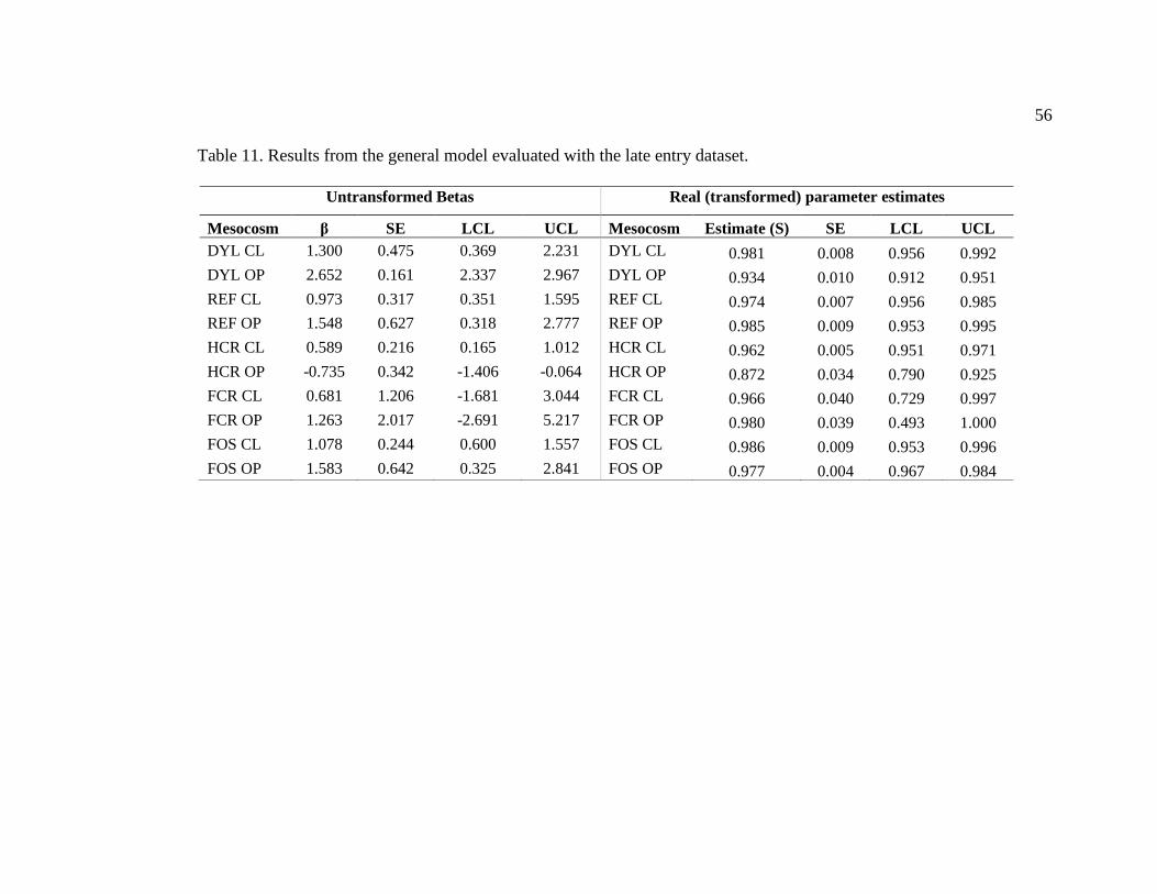
56
Table 11. Results from the general model evaluated with the late entry dataset.
Untransformed Betas Real (transformed) parameter estimates
Mesocosm β SE LCL UCL Mesocosm Estimate (S) SE LCL UCL
DYL CL 1.300 0.475 0.369 2.231 DYL CL 0.981 0.008 0.956 0.992
DYL OP 2.652 0.161 2.337 2.967 DYL OP 0.934 0.010 0.912 0.951
REF CL 0.973 0.317 0.351 1.595 REF CL 0.974 0.007 0.956 0.985
REF OP 1.548 0.627 0.318 2.777 REF OP 0.985 0.009 0.953 0.995
HCR CL 0.589 0.216 0.165 1.012 HCR CL 0.962 0.005 0.951 0.971
HCR OP -0.735 0.342 -1.406 -0.064 HCR OP 0.872 0.034 0.790 0.925
FCR CL 0.681 1.206 -1.681 3.044 FCR CL 0.966 0.040 0.729 0.997
FCR OP 1.263 2.017 -2.691 5.217 FCR OP 0.980 0.039 0.493 1.000
FOS CL 1.078 0.244 0.600 1.557 FOS CL 0.986 0.009 0.953 0.996
FOS OP 1.583 0.642 0.325 2.841 FOS OP 0.977 0.004 0.967 0.984


