
HAL Id: tel-01154565https://tel.archives-ouvertes.fr/tel-01154565
Submitted on 22 May 2015
HAL is a multi-disciplinary open accessarchive for the deposit and dissemination of sci-entific research documents, whether they are pub-lished or not. The documents may come fromteaching and research institutions in France orabroad, or from public or private research centers.
L’archive ouverte pluridisciplinaire HAL, estdestinée au dépôt et à la diffusion de documentsscientifiques de niveau recherche, publiés ou non,émanant des établissements d’enseignement et derecherche français ou étrangers, des laboratoirespublics ou privés.
Indexing and Searching for Similarities of Images withStructural Descriptors via Graph-cuttings Methods
Yi Ren
To cite this version:Yi Ren. Indexing and Searching for Similarities of Images with Structural Descriptors viaGraph-cuttings Methods. Computer science. Université de Bordeaux, 2014. English. NNT :2014BORD0215. tel-01154565

Indexing and Searching for Similarities of Images with StructuralDescriptors via Graph-cuttings Methods
Yi REN
LaBRI
Universite de Bordeaux
A thesis submitted for the degree of
PHD
October 2011 - September 2014
Supervised byProfesseure Jenny Benois-Pineau
Maıtre de conferences Aurelie Bugeau

Reviewer : Mr Bernard Merialdo and Mr Philippe-Henri Gosselin
Signature from author: Yi REN
ii

Contents
List of Figures iii
List of Tables xi
Glossary xvii
1 Introduction 1
1.1 Problems and Objectives . . . . . . . . . . . . . . . . . . . . . . . . . . . . . 2
1.2 Contributions . . . . . . . . . . . . . . . . . . . . . . . . . . . . . . . . . . . 3
1.3 Organization of the Thesis . . . . . . . . . . . . . . . . . . . . . . . . . . . . 3
2 Related Work 5
2.1 Image Descriptors . . . . . . . . . . . . . . . . . . . . . . . . . . . . . . . . . 5
2.1.1 Formalization . . . . . . . . . . . . . . . . . . . . . . . . . . . . . . . 6
2.1.2 Image Feature Detection . . . . . . . . . . . . . . . . . . . . . . . . . 7
2.1.3 Image Feature Extraction and Description . . . . . . . . . . . . . . . . 7
2.1.4 Local Image Descriptors . . . . . . . . . . . . . . . . . . . . . . . . . 8
2.1.5 Semi-local Image Descriptors . . . . . . . . . . . . . . . . . . . . . . 10
2.1.6 Global Image Descriptors . . . . . . . . . . . . . . . . . . . . . . . . 11
2.1.6.1 Color . . . . . . . . . . . . . . . . . . . . . . . . . . . . . . 11
2.1.6.2 Texture . . . . . . . . . . . . . . . . . . . . . . . . . . . . . 13
2.1.6.3 Gist . . . . . . . . . . . . . . . . . . . . . . . . . . . . . . 15
2.1.7 Similarity Metrics . . . . . . . . . . . . . . . . . . . . . . . . . . . . 16
2.2 Image Retrieval in the Real World . . . . . . . . . . . . . . . . . . . . . . . . 17
2.3 Image Representation . . . . . . . . . . . . . . . . . . . . . . . . . . . . . . . 18
2.3.1 The Bag-of-Words Model . . . . . . . . . . . . . . . . . . . . . . . . 19
iii

CONTENTS
2.3.2 The State-of-the-art to Improve the Bag-of-Visual-Words Model . . . . 21
2.3.2.1 Spatial pyramid image representation . . . . . . . . . . . . . 22
2.3.2.2 Superpixels . . . . . . . . . . . . . . . . . . . . . . . . . . 23
2.3.2.3 Using class-specific codebooks to vote for object position . . 24
2.3.2.4 Spatiograms versus Histograms . . . . . . . . . . . . . . . . 24
2.3.2.5 Spatial orientations of visual word pairs to improve Bag-of-
Visual-Words model . . . . . . . . . . . . . . . . . . . . . . 25
2.3.2.6 Improve BoW model with respect to feature encoding . . . . 25
2.3.3 Region-based Image Representation . . . . . . . . . . . . . . . . . . . 25
2.3.4 Graph-based Image Representation and its Applications . . . . . . . . 26
2.4 Conclusion . . . . . . . . . . . . . . . . . . . . . . . . . . . . . . . . . . . . 27
3 Graph-based Image Representation 29
3.1 An Overview of the Image Graph Model . . . . . . . . . . . . . . . . . . . . . 29
3.2 Weighted Image Graph Representation . . . . . . . . . . . . . . . . . . . . . . 30
3.3 Graph Construction . . . . . . . . . . . . . . . . . . . . . . . . . . . . . . . . 31
3.3.1 Graph Nodes Selection in Image Graph . . . . . . . . . . . . . . . . . 31
3.3.1.1 Prominent keypoints . . . . . . . . . . . . . . . . . . . . . . 31
3.3.1.2 Dense sampling strategy . . . . . . . . . . . . . . . . . . . . 31
3.3.2 Graph Edges Construction in Image Graph . . . . . . . . . . . . . . . 32
3.3.3 Graph Weights in Image Graph . . . . . . . . . . . . . . . . . . . . . 33
3.3.3.1 Color weight . . . . . . . . . . . . . . . . . . . . . . . . . . 34
3.3.3.2 Texture weight . . . . . . . . . . . . . . . . . . . . . . . . . 36
3.4 Graph Partitioning . . . . . . . . . . . . . . . . . . . . . . . . . . . . . . . . 37
3.4.1 Graph-based Image Segmentation Problem . . . . . . . . . . . . . . . 38
3.4.2 Image Graph Labeling Problem . . . . . . . . . . . . . . . . . . . . . 38
3.5 Graph Partitioning Approaches . . . . . . . . . . . . . . . . . . . . . . . . . . 39
3.5.1 Graph Cuts: energy-based method . . . . . . . . . . . . . . . . . . . . 39
3.5.1.1 Binary labeling . . . . . . . . . . . . . . . . . . . . . . . . 39
3.5.1.2 Extension to multi-label problems . . . . . . . . . . . . . . . 41
3.5.1.3 Graph Cuts from perspective of energy minimization . . . . 42
3.5.1.4 Seed selection . . . . . . . . . . . . . . . . . . . . . . . . . 45
3.5.1.5 Weakness . . . . . . . . . . . . . . . . . . . . . . . . . . . 45
iv

CONTENTS
3.5.1.6 Graph Cuts in applications . . . . . . . . . . . . . . . . . . 47
3.5.2 Normalized Cuts . . . . . . . . . . . . . . . . . . . . . . . . . . . . . 47
3.5.2.1 Basic concepts and theory . . . . . . . . . . . . . . . . . . . 47
3.5.2.2 Computing NCut by eigen-value decomposition . . . . . . . 49
3.5.2.3 The grouping algorithm description . . . . . . . . . . . . . . 50
3.5.2.4 Multiclass cuts of general weighted graph . . . . . . . . . . 50
3.5.2.5 Normalized Cuts in applications . . . . . . . . . . . . . . . 51
3.5.3 Kernel Based Multilevel Graph Clustering Algorithms . . . . . . . . . 52
3.5.3.1 The standard k-means clustering algorithm . . . . . . . . . . 52
3.5.3.2 Kernel k-means . . . . . . . . . . . . . . . . . . . . . . . . 53
3.5.3.3 Weighted kernel k-means . . . . . . . . . . . . . . . . . . . 54
3.5.3.4 Multilevel weighted kernel k-means algorithm . . . . . . . . 55
3.5.3.5 Kernel k-means in applications . . . . . . . . . . . . . . . . 58
3.6 Illustrations of Graph Partitioning . . . . . . . . . . . . . . . . . . . . . . . . 58
3.7 Conclusions . . . . . . . . . . . . . . . . . . . . . . . . . . . . . . . . . . . . 60
4 Bag-of-Bags of Words Model 71
4.1 Overview of the Bag-of-Bags of Words Model . . . . . . . . . . . . . . . . . . 71
4.1.1 Feature Extraction . . . . . . . . . . . . . . . . . . . . . . . . . . . . 72
4.1.2 Graph Construction . . . . . . . . . . . . . . . . . . . . . . . . . . . . 73
4.1.3 Irregular Subgraphs . . . . . . . . . . . . . . . . . . . . . . . . . . . . 74
4.1.4 Bag-of-Bags of Words Description . . . . . . . . . . . . . . . . . . . . 74
4.2 (Dis-)Similarity Measurement between Histograms . . . . . . . . . . . . . . . 75
4.3 BBoW on Single Level for Image Retrieval . . . . . . . . . . . . . . . . . . . 77
4.3.1 Co-occurrence Criteria . . . . . . . . . . . . . . . . . . . . . . . . . . 78
4.3.2 Weighted Bipartite Graph Matching . . . . . . . . . . . . . . . . . . . 79
4.4 Summary of the BBoW model for CBIR . . . . . . . . . . . . . . . . . . . . . 82
4.5 Discussion and Conclusion . . . . . . . . . . . . . . . . . . . . . . . . . . . . 83
5 Irregular Pyramid Matching 85
5.1 BBoW on Pyramid Level . . . . . . . . . . . . . . . . . . . . . . . . . . . . . 85
5.1.1 Graph Partitioning Scheme . . . . . . . . . . . . . . . . . . . . . . . . 85
5.1.2 Irregular Pyramid Matching . . . . . . . . . . . . . . . . . . . . . . . 86
5.2 BBoW on Pyramid Levels for Image Retrieval . . . . . . . . . . . . . . . . . . 86
v

CONTENTS
5.2.1 Similarity Measure . . . . . . . . . . . . . . . . . . . . . . . . . . . . 87
5.2.2 Global Algorithm for Image Retrieval with BBoW model . . . . . . . . 87
5.3 Discussion and Conclusion . . . . . . . . . . . . . . . . . . . . . . . . . . . . 88
6 Results and Discussion 91
6.1 Image Datasets . . . . . . . . . . . . . . . . . . . . . . . . . . . . . . . . . . 91
6.2 Experimental Settings . . . . . . . . . . . . . . . . . . . . . . . . . . . . . . . 93
6.2.1 Experimental Settings on SIVAL . . . . . . . . . . . . . . . . . . . . . 94
6.2.2 Experimental Settings on Caltech-101 . . . . . . . . . . . . . . . . . . 95
6.2.3 Experimental Settings on PPMI . . . . . . . . . . . . . . . . . . . . . 95
6.3 Evaluation Metrics . . . . . . . . . . . . . . . . . . . . . . . . . . . . . . . . 95
6.3.1 Performance Measures for Image Retrieval . . . . . . . . . . . . . . . 95
6.3.2 Partition Precision (PP) . . . . . . . . . . . . . . . . . . . . . . . . . . 97
6.4 Comparison of Co-occurrence Measures for Image Matching in the BBoW Model 98
6.5 Parameters Evaluation . . . . . . . . . . . . . . . . . . . . . . . . . . . . . . 102
6.5.1 Patch Size and Contribution of Color Term . . . . . . . . . . . . . . . 102
6.5.2 Influence of Texture Term . . . . . . . . . . . . . . . . . . . . . . . . 103
6.6 Influence of Neighbourhood Systems . . . . . . . . . . . . . . . . . . . . . . . 103
6.7 Influence of Distance Metric for Histogram Comparison . . . . . . . . . . . . 105
6.8 Irregular Graph Representation versus SPM for Image Retrieval . . . . . . . . 106
6.9 Partition Analysis . . . . . . . . . . . . . . . . . . . . . . . . . . . . . . . . . 109
6.9.1 Stability of Graph Partitions . . . . . . . . . . . . . . . . . . . . . . . 109
6.9.2 Quality of Subgraphs Matching . . . . . . . . . . . . . . . . . . . . . 114
6.10 Conclusion . . . . . . . . . . . . . . . . . . . . . . . . . . . . . . . . . . . . 118
7 Conclusion and Perspectives 119
7.1 Summary of the Work in this Dissertation . . . . . . . . . . . . . . . . . . . . 119
7.2 Future Work . . . . . . . . . . . . . . . . . . . . . . . . . . . . . . . . . . . . 121
7.2.1 Objective Functions in Edges Weights . . . . . . . . . . . . . . . . . . 121
7.2.2 Improving Segmentation Methods . . . . . . . . . . . . . . . . . . . . 121
7.2.3 Fusion across Graph Partitions . . . . . . . . . . . . . . . . . . . . . . 121
7.2.4 Applications of the BBoW Model . . . . . . . . . . . . . . . . . . . . 122
Appendix A Experimental Results in SIVAL 123
vi

CONTENTS
Appendix B Experimental Results in Caltech-101 129
Appendix C Experimental Results in PPMI 147
Appendix D Proofs 151
Appendix E Statistical Test 153
E.1 Paired samples t-interval . . . . . . . . . . . . . . . . . . . . . . . . . . . . . 153
E.2 Matched Paired t-test . . . . . . . . . . . . . . . . . . . . . . . . . . . . . . . 153
E.2.1 Data preparation . . . . . . . . . . . . . . . . . . . . . . . . . . . . . 154
E.3 Matched Paired t-test and interval . . . . . . . . . . . . . . . . . . . . . . . . 154
E.4 Measurement in theory . . . . . . . . . . . . . . . . . . . . . . . . . . . . . . 155
E.4.1 The limits of data in research . . . . . . . . . . . . . . . . . . . . . . . 155
E.4.2 Sample size . . . . . . . . . . . . . . . . . . . . . . . . . . . . . . . . 155
E.4.3 Data preparation . . . . . . . . . . . . . . . . . . . . . . . . . . . . . 156
E.4.4 The t distribution . . . . . . . . . . . . . . . . . . . . . . . . . . . . . 157
E.4.5 p-value method . . . . . . . . . . . . . . . . . . . . . . . . . . . . . . 157
E.4.5.1 Basic of Hypothesis Testing . . . . . . . . . . . . . . . . . . 157
E.4.5.2 Level of significance . . . . . . . . . . . . . . . . . . . . . . 158
E.4.5.3 A very rough guideline . . . . . . . . . . . . . . . . . . . . 158
E.4.5.4 Summary . . . . . . . . . . . . . . . . . . . . . . . . . . . . 159
References 161
vii

Abstract
Image representation is a fundamental question for several computer vision tasks.
The contributions discussed in this thesis extend the basic bag-of-words represen-
tations for the tasks of object recognition and image retrieval.
In the present thesis, we are interested in image description by structural graph
descriptors. We propose a model, named bag-of-bags of words (BBoW), to ad-
dress the problems of object recognition (for object search by similarity), and es-
pecially Content-Based Image Retrieval (CBIR) from image databases. The pro-
posed BBoW model, is an approach based on irregular pyramid partitions over
the image. An image is first represented as a connected graph of local features on
a regular grid of pixels. Irregular partitions (subgraphs) of the image are further
built by using graph partitioning methods. Each subgraph in the partition is then
represented by its own signature. The BBoW model with the aid of graphs, ex-
tends the classical bag-of-words (BoW) model by embedding color homogeneity
and limited spatial information through irregular partitions of an image.
Compared to existing methods for image retrieval, such as Spatial Pyramid Match-
ing (SPM), the BBoW model does not assume that similar parts of a scene always
appear at the same location in images of the same category. The extension of the
proposed model to pyramid gives rise to a method we named irregular pyramid
matching (IPM).
The experiments demonstrate the strength of our approach for image retrieval
when the partitions are stable across an image category. The statistical analysis
of subgraphs is fulfilled in the thesis. To validate our contributions, we report re-
sults on three related computer vision datasets for object recognition, (localized)
content-based image retrieval and image indexing. The experimental results in a
database of 13,044 general-purposed images demonstrate the efficiency and effec-
tiveness of the proposed BBoW framework.
Keywords : Computer vision, Pattern recognition, Image analysis, Image segmen-
tation, Graphs, Graph algorithms, Graph Cuts, Graph partitioning, Graph match-
ing, Kernel k-means, Clustering.
Resume
Dans cette these, nous nous interessons a la recherche d’images similaires avec
des descripteurs structures par decoupages d’images sur les graphes.
Nous proposons une nouvelle approche appelee “bag-of-bags of words” (BBoW)
pour la recherche d’images par le contenu (CBIR). Il s’agit d’une extension du
modele classique dit sac-de-mots (bag of words - BoW). Dans notre approche,
une image est representee par un graphe place sur une grille reguliere de pixels
d’image. Les poids sur les aretes dependent de caracteristiques locales de couleur
et texture. Le graphe est decoupe en un nombre fixe de regions qui constituent
une partition irreguliere de l’image. Enfin, chaque partition est representee par
sa propre signature suivant le meme schema que le BoW. Une image est donc
decrite par un ensemble de signatures qui sont ensuite combinees pour la recherche
d’images similaires dans une base de donnees. Contrairement aux methodes ex-
istantes telles que Spatial Pyramid Matching (SPM), le modele BBoW propose
ne repose pas sur l’hypothese que des parties similaires d’une scene apparaissent
toujours au meme endroit dans des images d’une meme categorie. L’extension
de cette methode a une approche multi-echelle, appelee Irregular Pyramid Match-
ing (IPM), est egalement decrite. Les resultats montrent la qualite de notre ap-
proche lorsque les partitions obtenues sont stables au sein d’une meme categorie
d’images. Une analyse statistique est menee pour definir concretement la notion
de partition stable.
Nous donnons nos resultats sur des bases de donnees pour la reconnaissance d’objets,
d’indexation et de recherche d’images par le contenu afin de montrer le caractere
general de nos contributions.

Mots-cles : Vision par ordinateur, Reconnaissance de formes, Analyse d’Image,
Segmentation d’Images, Graphes, Algorithmes de graphes, Coupe de graphes, Par-
titionnement de graphe, Appariement de graphes, Noyau k-means, Clustering.

This thesis is dedicated to my parents
Ren XianLiang and Ji XueLan
who have been offering me unconditional love and support from birth ...

Acknowledgements
I would firstly like to thank my two supervisors: Dr. Aurelie BUGEAU and Dr.
Jenny BENOIS-PINEAU, for their company over the past three years of Ph.D
program as I moved from an idea to a completed study.
I offer my sincere appreciation for the learning opportunities provided by my the-
sis jury composed of: Dr. Bernard MERIALDO, Dr. Philippe-Henri GOSSELIN,
Dr. Alan HANJALIC, Dr. Luc BRUN, Dr. Pascal DESBARATS. Their pertinent
advice helps to polish both this manuscript and presentation of my Ph.D viva voce.
In particular, I thank the reviewers, Professor Bernard MERIALDO and Professor
Philippe-Henri GOSSELIN for proofreading the thesis; their remarks inspired me
to adopt statistical test as more convincing measurement for experiments valida-
tion.
I would like to express my deepest gratitude to Dr. Kaninda MUSUMBU, Dr.
Stefka GUEORGUIEVA, Dr. Pascal DESBARATS, Dr. Nicolas HANUSSE, Dr.
Pascal WEIL in my laboratory LaBRI: their encouragement when the times got
rough are much appreciated and duly noted.
I would also like to thank all my teachers in University of Caen, for generously
sharing their time, ideas and dedications during my studies in Master. All valu-
able knowledge they have taught me built my solid foundation in this domain and
contribute what I am today...
This Ph.D research program was supported by CNRS (Centre national de la recherche
scientifique) of France & Region of Aquitaine Grant.
List of Figures
2.1 An example of image descriptor components. The similarities or distances
between images are based on the similarities or distances between the image
feature vectors being extracted. Different types of feature vectors may require
different similarity functions. Furthermore, different similarity/distance func-
tions can be applied to the same feature set. The figure is excerpted from
Penatti et al.[1]. . . . . . . . . . . . . . . . . . . . . . . . . . . . . . . . . . . 7
2.2 The major stages for extracting SIFT features. (a) Scale-space extrema de-
tection. (b) Orientation assignment. (c) Keypoint descriptor. The figures are
extracted from Lowe’s paper [2]. . . . . . . . . . . . . . . . . . . . . . . . . . 8
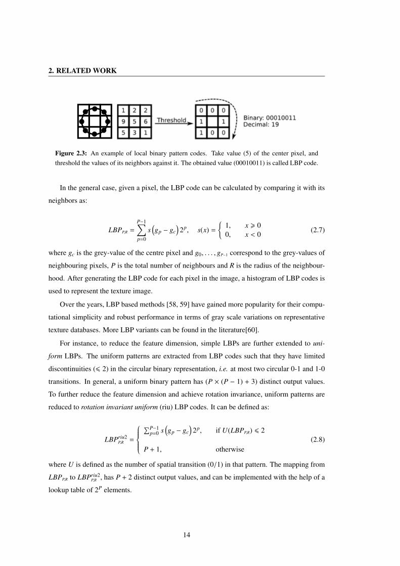
2.3 An example of local binary pattern codes. Take value (5) of the center pixel,
and threshold the values of its neighbors against it. The obtained value (00010011)
is called LBP code. . . . . . . . . . . . . . . . . . . . . . . . . . . . . . . . . 14
2.4 An overview of the many facets of image retrieval as field of research. The
figures are extracted from Dattas paper [3]. . . . . . . . . . . . . . . . . . . . 18
2.5 The Bag of Words model. The left-most picture illustrates the Bag of Words
in document. Other pictures show the Bag of Visual Words in image. These
pictures are excerpted from the source of S.Lazebnik.1 . . . . . . . . . . . . . 20
2.6 The Bag-of-Visual Words (BoVW) image representation. The figure is from
the source of S.Lazebnik.2 . . . . . . . . . . . . . . . . . . . . . . . . . . . . 21
iii

LIST OF FIGURES
2.7 An example of constructing a three-level pyramid. The image has three feature
types, indicated by circles, diamonds, and crosses. At the top, the SPM method
subdivides the image at three different levels of resolution. Next, for each level
of resolution and each grid cell, SPM counts the features that fall in each spatial
bin. Finally, SPM weights each spatial histogram according to Equation (2.17).
The figure is excerpted from Lazebnik et al. [4]. . . . . . . . . . . . . . . . . . 22
2.8 An example of superpixels. (a) Input image. (b) A “superpixel” map with 200
superpixels via Normalized Cuts algorithm [5]. The figure is excerpted from
Mori et al. [6]. . . . . . . . . . . . . . . . . . . . . . . . . . . . . . . . . . . . 23
2.9 A hierarchy of “nested” Graph Words on four layers (on the left) in the same
example of image (on the right). Seed is marked as hollow circle in white color,
and neighbour nodes are shown as solid circles in black color. The figures are
extracted from [7]. . . . . . . . . . . . . . . . . . . . . . . . . . . . . . . . . 28
3.1 An overview of the processing chain for the proposed image graph model. (I) Image
is represented by an initial weighted graph. (II) Graph partitioning consists in finding
the optimal labeling for each graph nodes. (III) Find the best bipartite matched sub-
graphs between images pairs (IV) Retrieve images based on signatures that define the
similarities between these subgraphs. . . . . . . . . . . . . . . . . . . . . . . . . 30
3.2 Graph construction. (a) Initial SURF keypoints. (b) Filtered keypoints. (c)
Seeds selection. (d) Delaunay triangulation over filtered feature points. (e)
Graph-cuts result. (f) Labeling result. . . . . . . . . . . . . . . . . . . . . . . 32
3.3 Options for the neighbourhood system of image graph. . . . . . . . . . . . . . 33
3.4 Block DCT on 8 × 8 pixel patch. . . . . . . . . . . . . . . . . . . . . . . . . . . 36
3.5 A block of 8 × 8 pixel on DCT, the solid dot in black denotes the graph node, the 64
DCT coefficients are scanned in a “zig-zag” fashion. . . . . . . . . . . . . . . . . . 36
3.6 The DCT (Discrete Cosine Transform) block is scanned in a diagonal zigzag pattern
starting at the DC coefficient d(0,0) to produce a list of quantized coefficient values.
Here only five AC coefficients d(1,0), d(0,1), d(0,2), d(1,1), d(2,0) in luma (Y’) com-
ponent of YUV system are considered due to their good discriminative properties. . . . 37
iv

LIST OF FIGURES
3.7 An example of binary labeling on an image graph via Graph Cuts. The graph
corresponds to an image that consists of a 3 × 3 pixels set P, with observed
color intensities Ip in certain color space for each p ∈ P. Given binary labels
L = 0, 1, an optimal labeling L assigns label lp ∈ L to each pixel p. One part
of this image is excerpted from [8]. . . . . . . . . . . . . . . . . . . . . . . . . 40
3.8 Example of α-β swap and α-expansion. (a) initial labeling: α in red, β in
green, γ in blue. (b) α-β swap: only number of pixels with label α or β change
their labels, pixels with label γ remain unchanged. (c) α-expansion: pixels
with different labels can change their labels simultaneously. The figures are
excerpted from [9]. This figure is better viewed in color. . . . . . . . . . . . . 42
3.9 Seed points are in hollow circle of different colors. The graph nodes are in red
solid points. . . . . . . . . . . . . . . . . . . . . . . . . . . . . . . . . . . . . 45
3.10 Examples of seeds selection in prominent keypoints approach. The stability of
seeds is hardly reached due to the uncontrolled nature of the images available.
All examples of images are from SIVAL dataset [10]. There are three seeds in
each image, and these seeds are labelled with their own colors (in red, orange
and yellow). This figure is better viewed in color. . . . . . . . . . . . . . . . . 46
3.11 An overview of the kernel-based multilevel algorithm for graph clustering pro-
posed by Dhillon et al. [11], here K = 6. A part of this image is excerpted
from [12]. . . . . . . . . . . . . . . . . . . . . . . . . . . . . . . . . . . . . . 56
3.12 Examples of graph partitioning in 4 irregular subgraphs on five examples in
category “accordion” from Caltech-101 dataset by three methods: Graph Cuts
(GC), Normalized Cut (NC), kernel k-means (KKM). This figure is better viewed
in color. . . . . . . . . . . . . . . . . . . . . . . . . . . . . . . . . . . . . . . 59
3.13 Examples of graph partitioning in 4 irregular subgraphs on five examples in
category “faces” from Caltech-101 dataset by three methods: Graph Cuts (GC),
Normalized Cut (NC), kernel k-means (KKM). This figure is better viewed in
color. . . . . . . . . . . . . . . . . . . . . . . . . . . . . . . . . . . . . . . . 60
3.14 Examples of graph partitioning in 4 irregular subgraphs on five examples in cat-
egory “pagoda” from Caltech-101 dataset by three methods: Graph Cuts (GC),
Normalized Cut (NC), kernel k-means (KKM). This figure is better viewed in
color. . . . . . . . . . . . . . . . . . . . . . . . . . . . . . . . . . . . . . . . 61
v

LIST OF FIGURES
3.15 Examples of graph partitioning in 4 irregular subgraphs on five examples in cat-
egory “trilobite” from Caltech-101 dataset by three methods: Graph Cuts (GC),
Normalized Cut (NC), kernel k-means (KKM). This figure is better viewed in
color. . . . . . . . . . . . . . . . . . . . . . . . . . . . . . . . . . . . . . . . 62
3.16 Examples of graph partitioning in 4 irregular subgraphs on five examples in
category “cellphone” from Caltech-101 dataset by three methods: Graph Cuts
(GC), Normalized Cut (NC), kernel k-means (KKM). This figure is better viewed
in color. . . . . . . . . . . . . . . . . . . . . . . . . . . . . . . . . . . . . . . 63
3.17 Examples of graph partitioning in 4 irregular subgraphs on five examples in
category “motorbikes” from Caltech-101 dataset by three methods: Graph Cuts
(GC), Normalized Cut (NC), kernel k-means (KKM). This figure is better viewed
in color. . . . . . . . . . . . . . . . . . . . . . . . . . . . . . . . . . . . . . . 64
3.18 Examples of graph partitioning in 16 irregular subgraphs on five examples
in category “accordion” from Caltech-101 dataset by three methods: Graph
Cuts (GC), Normalized Cut (NC), kernel k-means (KKM). This figure is better
viewed in color. . . . . . . . . . . . . . . . . . . . . . . . . . . . . . . . . . . 65
3.19 Examples of graph partitioning in 16 irregular subgraphs on five examples in
category “faces” from Caltech-101 dataset by three methods: Graph Cuts (GC),
Normalized Cut (NC), kernel k-means (KKM). This figure is better viewed in
color. . . . . . . . . . . . . . . . . . . . . . . . . . . . . . . . . . . . . . . . 66
3.20 Examples of graph partitioning in 16 irregular subgraphs on five examples in
category “pagoda” from Caltech-101 dataset by three methods: Graph Cuts
(GC), Normalized Cut (NC), kernel k-means (KKM). This figure is better viewed
in color. . . . . . . . . . . . . . . . . . . . . . . . . . . . . . . . . . . . . . . 67
3.21 Examples of graph partitioning in 16 irregular subgraphs on five examples in
category “trilobite” from Caltech-101 dataset by three methods: Graph Cuts
(GC), Normalized Cut (NC), kernel k-means (KKM). This figure is better viewed
in color. . . . . . . . . . . . . . . . . . . . . . . . . . . . . . . . . . . . . . . 68
3.22 Examples of graph partitioning in 16 irregular subgraphs on five examples
in category “cellphone” from Caltech-101 dataset by three methods: Graph
Cuts (GC), Normalized Cut (NC), kernel k-means (KKM). This figure is better
viewed in color. . . . . . . . . . . . . . . . . . . . . . . . . . . . . . . . . . . 69
vi

LIST OF FIGURES
3.23 Examples of graph partitioning in 16 irregular subgraphs on five examples
in category “motorbikes” from Caltech-101 dataset by three methods: Graph
Cuts (GC), Normalized Cut (NC), kernel k-means (KKM). This figure is better
viewed in color. . . . . . . . . . . . . . . . . . . . . . . . . . . . . . . . . . . 70
4.1 The diagram of construction of Bag-of-Bags of Words model. . . . . . . . . . . . . 72
4.2 The dense points sampling approach in BBoW model. . . . . . . . . . . . . . . 73
4.3 The obtained irregular subgraphs via graph partitioning. . . . . . . . . . . . . . 75
4.4 The “Bag-of-Bags of Words” description. . . . . . . . . . . . . . . . . . . . . 76
4.5 Examples of image graph partitions from category ‘accordion’ in Caltech-101
dataset. The partitions of 4 subgraphs are visible in the first row of the figure.
The second row of the figure shows 16 subgraphs in the partitioning. The nodes
in each subgraph are labelled with the same color. This figure is better viewed
in color. . . . . . . . . . . . . . . . . . . . . . . . . . . . . . . . . . . . . . . 80
4.6 Find optimal subgraph matching via Hungarian algorithm. . . . . . . . . . . . . . . 82
4.7 An optimal assignment for a given cost matrix. . . . . . . . . . . . . . . . . . . . . 82
4.8 The process of CBIR from database in BBoW model. . . . . . . . . . . . . . . 82
5.1 A schematic illustration of the BBoW representation at each level of the pyra-
mid. At level 0, the decomposition has a single graph, and the representation
is equivalent to the classical BoW. At level 1, the image is subdivided into four
subgraphs, leading to four features histograms, and so on. Each subgraph is
represented by its own color in this figure. This figure is better viewed in color. 86
5.2 The comparison of partitioning scheme between SPM and BBoW. At the left
side of the figure shows the partitioning scheme of Spatial Pyramid Matching
(SPM). At the right side of the figure illustrates the partitioning scheme of
the BBoW. Contrary to SPM with nested regular partitions, our partitions are
irregular and independent at each level. We keep the same resolution of the
image across multilevel. This figure is better viewed in color. . . . . . . . . . . 89
6.1 Example images from the SIVAL database. . . . . . . . . . . . . . . . . . . . . 92
6.2 A snapshot of images from Caltech-101. . . . . . . . . . . . . . . . . . . . . . 93
6.3 A snapshot of images from PPMI+ of the PPMI dataset that contains a person
playing the instrument. . . . . . . . . . . . . . . . . . . . . . . . . . . . . . . 93
vii

LIST OF FIGURES
6.4 Comparison of a series of image similarity measures. . . . . . . . . . . . . . . 99
6.5 Comparision between BoW and BBoW on SIVAL benchmark. (a) The precision-
recall curve for a “good” category : “stripednotebook”. (b) The precision-recall
curve for a “bad” category : “banana”. (c) Graph descriptors from “stripednote-
book”. (d) Graph descriptors from “banana”. . . . . . . . . . . . . . . . . . . 100
6.6 Two examples of graph partioning via Graph Cuts. The first row shows re-
sult of image ‘AjaxOrange079.jpg’, the second row is result of image ‘Ajax-
Orange049.jpg’. Both of images are from category “AjaxOrange” in SIVAL
dataset. (a)(d) Seeds. (b)(e) Initial image graph with chosen seeds. (c)(f) La-
beling result. . . . . . . . . . . . . . . . . . . . . . . . . . . . . . . . . . . . 101
6.7 An example of image graph partitions on the image minaret0032.jpg from
Caltech-101 dataset, when joint color-texture is embedded in edge weights.
The 1th - 4th columns correspond to graph partitions by setting α = 0, 0.5, 0.8, 1
in Equation (E.1) severally. The first row of this figure shows the results of
partitions at resolution r = 1, where each image is composed of 4 subgraphs.
The second row corresponds to 16 partitions at resolution r = 2, i.e. 16 sub-
graphs per image. This figure is better viewed in color. . . . . . . . . . . . . . 104
6.8 Example of graph partitions of two images as texture factor is considered in
edge weights under different neighbourhood systems. This figure is better
viewed in color. . . . . . . . . . . . . . . . . . . . . . . . . . . . . . . . . . . 105
6.9 The margin of mean Average Precision (mAP) for not surpassing categories in Caltech-
101 dataset. The margin =mAP(S PM)−mAP(KKM)
mAP(KKM) %. . . . . . . . . . . . . . . . . . . . 108
6.10 Mean Average Precision for surpassing categories in Caltech-101 dataset. . . . . . . . 108
6.11 The mean Average Precision for 16 typical categories in Caltech101 . . . . . . 109
6.12 The first row shows the 4 irregular subgraphs from “good” query images at
level 1. The second row shows the 4 irregular subgraphs from “bad” query
images at level 1. The nodes of individual subgraphs are labelled with the
same color (in red, blue, green, brown). This figure is better viewed in color. . . 113
6.13 A case study of BBoW (via Normalized Cuts). The precision of 8 typical query
images: 1st-4th query images are from a “good” category - minaret, 5th-8th
query images are from “bad” categories: cellphone and dollar bill. . . . . . . . 114
viii

LIST OF FIGURES
6.14 A case study of BBoW (via Graph Cuts). The precision of 8 typical query
images: 1st-4th query images are from a “good” category - minaret, 5th-8th
query images are from “bad” categories: cellphone and dollar bill. . . . . . . . 115
6.15 A case study of BBoW (via Kernel k-means). The precision of 8 typical query
images: 1st-4th query images are from a “good” category - minaret, 5th-8th
query images are from “bad” categories: cellphone and dollar bill. . . . . . . . 116
6.16 The mean and standard deviation of nodes’ numbers of corresponding sub-
graphs for intra-category, for 8 typical queries in Caltech-101 dataset - at single
level 1, i.e. 4 subgraphs. . . . . . . . . . . . . . . . . . . . . . . . . . . . . . 117
A.1 The overall Precision-Recall curve for a comparison between BBoVW and
BoVW in SIVAL dataset [10]. BBoVW: Bag-of-Bags of Visual Word. BoVW:
Bag-of-Visual Words. Each image is composed of 4 subgraphs in BBoW. The
dictionary of size 1000, as described in Section 6.2.1 of the Chapter 6, is learnt
over 30 sample images per class using k-means. The query images are chosen
from the rest of the SIVAL dataset for retrieval. In this figure, the red curve
corresponds to application of co-occurrence measure defined in Equation (4.4)
for image matching in the BBoW Model. The blue/red curve correspond to
BoVW with/without points filtration. . . . . . . . . . . . . . . . . . . . . . . . 124
A.2 A complete comparison of similarity measures by using co-occurrence criteria
in BBoW, as defined in Section 4.3.1 of the Chapter 4. Each image is composed
of 4 subgraphs. There are six curves in this figure: “Min Histogram Distances”
with respect to Equation (4.4) (Curve 1), “Sum-of-mins Histogram Distances”
with respect to Equation (4.5) (Curve 2), “Sum-of-maxima Histogram Dis-
tances” with respect to Equation (4.9) (Curve 3), “Sums of Histogram Dis-
tances” with respect to Equation (4.8) (Curve 4), “Sum-of-means Histogram
Distances” with respect to Equation (4.6) (Curve 5), “Sum-of-medians His-
togram Distances” with respect to Equation (4.7) (Curve 6). The Curve 4 and
5 are coincident. . . . . . . . . . . . . . . . . . . . . . . . . . . . . . . . . . . 125
A.3 The category-based Precision-Recall curve for 25 categories in SIVAL dataset. . 128
B.1 Retrieval results of image “faces0032”. This figure is better viewed in color. . . 140
B.2 Retrieval results of image “faces0036”. This figure is better viewed in color. . . 141
B.3 Retrieval results of image “faces0038”. This figure is better viewed in color. . . 142
ix

LIST OF FIGURES
B.4 Retrieval results of image “faces0039”. This figure is better viewed in color. . . 143
B.5 Retrieval results of image “faces0049”. This figure is better viewed in color. . . 144
B.6 The distribution of average precision values for query images in 19 surpassing
classes + a category “car side” that only contains grayscale images, on the
whole Caltech-101 dataset. The comparison is evaluated between SPM and
BBoW (KKM) at level 1. Each image is partitioned into 4 subgraphs. . . . . . . 146
x

List of Tables
3.1 Examples of commonly used kernel functions. . . . . . . . . . . . . . . . . . . 54
6.1 The basic notions for information retrieval systems. . . . . . . . . . . . . . . . 96
6.2 Influence of parameter λ (Equation (3.4)) on image retrieval. For each value,
the mean average precision is given. For this experiment, the patch size is set
to n = 5. . . . . . . . . . . . . . . . . . . . . . . . . . . . . . . . . . . . . . . 102
6.3 Influence of parameter n (section 3.3.3.1) on image retrieval. For each value,
the mean average precision is given. For this experiment, λ = 5. . . . . . . . . 102
6.4 Evaluation of embedding joint color-texture energy in graph weights for image
retrieval. Graph weights account for more color features as value of parameter
α in Equation (E.1) increases. The mAPs are given for each single level and
pyramid. The patch size is set to n = 5. λ = 5. The size of visual codebook is
400. By contrast, the mAP for SPM is 0.409. . . . . . . . . . . . . . . . . . . 103
6.5 The influence of distance metrics to compute a cost matrix for graph matching
via Hungarian algorithm. Note that the partitions are obtained by KKM. The
experiments were run in PPMI dataset, and its settings have been described in
Section 6.2.3. . . . . . . . . . . . . . . . . . . . . . . . . . . . . . . . . . . . 105
6.6 The retrieval performance (mAP ± standard deviation of APs) on PPMI dataset. 106
6.7 Retrieval performance on subset of Caltech-101 dataset composed of 2945
query images and 5975 images from database for retrieval. We set α = 1 in
Equation (E.1), i.e. only consider color-related term wCpq in wpq. A postscript:
SPM wins BBoW (with KKM) by a small margin with a mAP value of 0.14,
versus 0.1327 for KKM, while SPM has higher std as value of 0.0660. . . . . . 107
xi
LIST OF TABLES
6.8 The comparison of mAPs for BBoW (via GC) vs BBoW (via NCuts) vs BBoW
(via KKM) vs SPM on 4 partitions of five examples of images from category
“accordion”. See Figure 3.12. . . . . . . . . . . . . . . . . . . . . . . . . . . 111
6.9 The comparison of mAPs for BBoW (via GC) vs BBoW (via NCuts) vs BBoW
(via KKM) vs SPM on 4 partitions of five examples of images from category
“faces”. See Figure 3.13. . . . . . . . . . . . . . . . . . . . . . . . . . . . . . 111
6.10 The comparison of mAPs for BBoW (via GC) vs BBoW (via NCuts) vs BBoW
(via KKM) vs SPM on 4 partitions of five examples of images from category
“pagoda”. See Figure 3.14. . . . . . . . . . . . . . . . . . . . . . . . . . . . . 111
6.11 The comparison of mAPs for BBoW (via GC) vs BBoW (via NCuts) vs BBoW
(via KKM) vs SPM on 4 partitions of five examples of images from category
“trilobite”. See Figure 3.15. . . . . . . . . . . . . . . . . . . . . . . . . . . . 112
6.12 The comparison of mAPs for BBoW (via GC) vs BBoW (via NCuts) vs BBoW
(via KKM) vs SPM on 4 partitions of five examples of images from category
“cellphone”. See Figure 3.16. . . . . . . . . . . . . . . . . . . . . . . . . . . . 112
6.13 The comparison of mAPs for BBoW (via GC) vs BBoW (via NCuts) vs BBoW
(via KKM) vs SPM on 4 partitions of five examples of images from category
“motorbikes”. See Figure 3.17. . . . . . . . . . . . . . . . . . . . . . . . . . . 112
6.14 The PP Precision(Γkj)k=1,2,3,4 = P(g j,k)k=1,2,3,4 of corresponding subgraphs
for 4 typical “good” queries. Method: BBoW via Normalized Cut. . . . . . . . 115
6.15 The PP Precision(Γkj)k=1,2,3,4 = P(g j,k)k=1,2,3,4 of corresponding subgraphs
for 4 typical “bad” queries. Method: BBoW via Normalized Cut. . . . . . . . . 116
6.16 The mean of node numbers and its standard deviation for corresponding matched
subgraphs of intra-category minaret, for 4 typical good queries in Caltech-101
dataset, at single level 1, i.e. 4 subgraphs. Method: BBoW via Normalized Cut. 117
6.17 The mean of node numbers and its standard deviation for corresponding matched
subgraphs of intra-category cellphone and dollar bill, for 4 typical bad queries
in Caltech-101 dataset, at single level 1, i.e. 4 subgraphs. Method: BBoW via
Normalized Cut. . . . . . . . . . . . . . . . . . . . . . . . . . . . . . . . . . . 117
6.18 The P(g j,k)k=1,...,4 of corresponding subgraphs for 4 typical “good” queries.
Method: BBoW via Normalized Cut. . . . . . . . . . . . . . . . . . . . . . . . 118
6.19 The P(g j,k)k=1,...,4 of corresponding subgraphs for 4 typical “bad” queries.
Method: BBoW via Normalized Cut. . . . . . . . . . . . . . . . . . . . . . . . 118
xii
LIST OF TABLES
A.1 The precision-recall values of experimental results, as complementary infor-
mation of Figure A.2. The experiments were run in SIVAL dataset with the aim
of comparing a series of similarity measures (co-occurrence criteria) versus the
classical bag-of-words model for image retrieval. The fist column lists recall
values ranging from 0 to 1.0 of 11 intervals. The 2nd-8th columns correspond
to the precision values for seven different measures. They are (1) Bag-of-
Words (BoW), without filtering points in graph nodes selection; (2) BoW, select
graph nodes by points filtration; (3) Bag-of-Bag-of-Visual-Words (BBoVW),
using Equation (4.4); (4) BBoVW, using Equation (4.5); (5) BBoVW, using
Equation (4.6) or its equivalent by using Equation (4.8); (6) BBoVW, using
Equation (4.7); (7) BBoVW, using Equation (4.9) respectively. . . . . . . . . . 126
B.1 KKM versus SPM at single level 1 (4 partitions per image). Performance
is measured by calculating the mean Average Precision (mAP) for category-
based queries. In addition, the mean of Standard deviation (Std) of Average
Precisions (APs) for category-based queries is given. The class names of 20
surpassing categories in which BBoW outperforms SPM are in bold in this table.130
B.2 Evaluation of BBoW via KKM in Caltech-101 dataset. Retrieval performance
was evaluated in mean Average Precision (mAP) on subset of Caltech-101
dataset composed of 2945 query images and 5975 images from database for
retrieval. The size of codebook is 400. . . . . . . . . . . . . . . . . . . . . . . 134
B.3 Evaluation of BBoW (via GC) vs BBoW (via NCuts) vs SPM in Caltech-
101 dataset. Retrieval performance was evaluated in mean Average Precision
(mAP) on subset of Caltech-101 dataset composed of 2945 query images and
5975 images from database for retrieval. The size of codebook is 400. The
highest results for each kind of level are shown in bold. . . . . . . . . . . . . . 134
B.4 Retrieval result of image faces0032. There are 5975 images from a subset of
Caltech-101 dataset for retrieval. Each image is partitioned into 4 subgraphs.
The file extension of each image is omitted. The size of codebook is 400. . . . 135
B.5 Retrieval result of image faces0036. There are 5975 images from a subset of
Caltech-101 dataset for retrieval. Each image is partitioned into 4 subgraphs.
The file extension of each image is omitted. The size of codebook is 400. . . . 136
xiii

LIST OF TABLES
B.6 Retrieval result of image faces0038. There are 5975 images from a subset of
Caltech-101 dataset for retrieval. Each image is partitioned into 4 subgraphs.
The file extension of each image is omitted. The size of codebook is 400. . . . 137
B.7 Retrieval result of image faces0039. There are 5975 images from a subset of
Caltech-101 dataset for retrieval. Each image is partitioned into 4 subgraphs.
The file extension of each image is omitted. The size of codebook is 400. . . . 138
B.8 Retrieval result of image faces0049. There are 5975 images from a subset of
Caltech-101 dataset for retrieval. Each image is partitioned into 4 subgraphs.
The file extension of each image is omitted. The size of codebook is 400. . . . 139
C.1 The retrieval performance (mAP) on PPMI dataset, using L1 distance as cost
matrix value for graph matching via Hungarian algorithm. . . . . . . . . . . . 148
C.2 The retrieval performance (mAP) on PPMI dataset, using L2 distance as cost
matrix value for graph matching Hungarian algorithm. . . . . . . . . . . . . . 149
xiv

List of Algorithms
1 Max-flow/Min-cut Algorithm . . . . . . . . . . . . . . . . . . . . . . . . . . . 41
2 Graph clustering by weighted kernel k-means . . . . . . . . . . . . . . . . . . 55
3 Graph clustering in coarsening phase . . . . . . . . . . . . . . . . . . . . . . . 57
4 Image comparison via the co-occurrence criteria . . . . . . . . . . . . . . . . . 79
5 Image comparison via Hungarian algorithm to reorganize histograms . . . . . 83
xv

GLOSSARY
xvi

Glossary
[X,Y]T A set of the corresponding coordinates for a set of feature points or pixels of an image P
νI A feature vector or descriptor
C = C1, . . . , CB A codebook or visual dictionary of size B
I A unit matrix with ones on the main diagonal and zeros elsewhere
L A set of labels
P An optimal partition of an image graph
δ() Kronecker’s delta
ΓKj = Γk
jk=1, ..., K = g1j , . . . , gK
j K-way partitioning for Image I j
κ A kernel function
K A kernel matrix
Pl A subset of graph nodes assigned label l in an image graph
Z∗ The set of non-negative integers
Ω Image database
πk The k-th cluster for the clustering πkKk=1
ρ Rank
πkKk=1 A clustering with k clusters
g j,kk=1, ..., K The subgraphs in image I j on single level of graph partitions
grj,kk=1, ..., Kr The subgraphs in image I j at resolution r on pyramid level of graph partitions
aiNi=1 A set of vectors that the k-means algorithm seeks to cluster
B The number of bins in codebook
G Graph
xvii

GLOSSARY
G j An undirected weighted graph constructed on the image I j
I(p) The color vector at point p
Ic(p) The intensity of a node or pixel p in color channel c
Ii, I j Images
K The number of clusters
Kr The fixed number of subgraphs at resolution r of graph partitions
p, q Nodes in a graph, or pixels in an image
R The resolution of a pyramidal partition
S A set of seeds
xp, yp The intrinsic coordinates (x,y) of the node or the pixel p
In×n(p) mean color vector at point p (over a n×n patch)
N(p) The neighbourhood of p
L An optimal joint labeling
P A set of feature points or pixels of an image
E j Graph edges of image I j
V j A set of vertices of image I j
BoF Bags of Features
CBIR Content-Based Image Retrieval, also known as query by image content (QBIC) and content-based visual information retrieval (CBVIR), is the application of computer vision techniquesto the image retrieval problem, that is, the problem of searching for digital images in largedatabases.
Gram matrix A matrix G = VT V , where V is a matrix whose column are the vectors vk.
HA Hard Assignment
ISM Implicit Shape Model [13]
mAP mean Average Precision
metric A metric on a set X is a function d : X × X → R that is required to satisfy conditions ofnon-negativity, identity, symmetry and sub additivity.
RGB Red, Green, Blue color space
ROC Receiver Operating Characteristic
xviii

GLOSSARY
ROI Region of Interest
SA Soft Assignment
Segmentation In computer vision, segmentation refers to the process of partitioning a digital imageinto multiple segments (sets of pixels).
Semi-supervised Learning In computer science, semi-supervised learning is a class of machine learn-ing techniques that make use of both labelled and unlabelled data for training - typically asmall amount of labelled data with a large amount of unlabelled data.
SIFT Scale-invariant feature transform (SIFT) is an algorithm in computer vision to detect anddescribe local features in images. The algorithm was published by David Lowe in 1999.
SPM Spatial Pyramid Matching
SURF Speeded Up Robust Features, which is a robust local feature detector, proposed by HerbertBay et al. in 2006
SVM Support Vector Machine
YUV Color space, which is composed of luma (Y’) and two chrominance (U,V) components.
xix

GLOSSARY
xx

Chapter 1
Introduction
Object detection and recognition remain outstanding problems for which there is no off-the-
shelf solution, despite a vast amount of literature on the subject. The problem is challenging
since characterizing the appearance of an object does not only involve the object itself but
also extrinsic factors such as illumination, relative position or even cluttered background in the
target image. Currently, object detection and recognition are typically considered as “retrieval”
task over a database of images, where content-based image retrieval is one of the core problems.
Content Based Image Retrieval (CBIR), as its name implies, consists in browsing, search-
ing and navigation of images from image databases based on their visual contents. CBIR has
been an active area of research for more than a decade. Traditional CBIR systems use low level
features like color, texture, shape and spatial location of objects to index and retrieve images
from databases. Low level features can be global or local (region based). Global feature based
CBIR fails to compare the regions or objects in which a user may be interested. Therefore
Region Based Image Retrieval (RBIR) is more effective in reflecting the user requirement. A
detailed survey of CBIR techniques can be found in the literature [3, 14, 15].
Recent methods in Content-Based Image Retrieval (CBIR) mostly rely on the bag-of-
visual-words (BoW) model [16]. The idea, borrowed from document processing, is to build
a visual codebook from all the feature points in a training image dataset. Each image is then
represented by a signature, which is a histogram of quantized visual features-words from the
codebook. Image features are thus considered as independent and orderless. The traditional
BoW model does not embed spatial layout of local features in the image signature. However,
this information has shown to be very useful in tasks like image retrieval, image classification,
and video indexing. Ren et al. [17] put forward a concept of grouping pixels into “superpixels”.
1

1. INTRODUCTION
Leibe et al. proposed to adopt codebooks to vote for object position [13]. Birchfield et al. [18]
introduced the concept of a spatiogram, which generalizes the histogram to allow higher-order
spatial moments to be part of the descriptor. Agarwal et al. [19] proposed “hyperfeatures”, a
multilevel local coding. More specifically, hyperfeatures are based on local histogram model
encoding co-occurrence statistics within each local neighborhood on multilevel image repre-
sentations. Lazebnik et al. [4] partitioned an image into increasingly fine grids and computed
histograms for each grid cell. The resulting spatial pyramid matching (SPM) method clearly
improves the BoW representation. Nevertheless, this method relies on the assumption that a
similar part of a scene generally appears at the same position across different images, which
does not always hold. Recently, many efforts can be found in the literature, e.g. the Fisher
vectors etc. [20, 21] that compete with SPM to give extensions of bag-of-words image repre-
sentations to encode spatial layout.
Graphs are versatile tools to conveniently represent patterns in computer vision applications
and they have been vastly investigated. By representing images with graphs, measuring the
similarities between images becomes equivalent to finding similar patterns inside series of
attributed (sub)graphs representing them. Duchenne et al. [22] introduced an approximate
algorithm based on graph-matching kernel for category-level image classification. Gibert et
al. [23] proposed to apply graph embedding in vector spaces by node attribute statistics for
classification. Bunke et al. [24] provided an overview of the structural and statistical pattern
recognition, and elaborated some of these attempts, such as graph clustering, graph kernels and
embedding etc., towards the unification of these two approaches.
1.1 Problems and Objectives
The thesis addresses issues of image representation for object recognition and categoriza-
tion from images. Compared with the seminal work by Lazebnik et al. [4], we try to address
a challenging question: will an irregular segmentation-like partition of images outperform a
regular partition (SPM)? Intuitively, it is invariant to the rotation and reasonable shift transfor-
mations of image plane. Nevertheless, what can be its resistance to noise and occlusions? How
will it compete with SPM when embedded into pyramidal paradigm?
2

1.2 Contributions
1.2 Contributions
This thesis presents a new approach for Content-Based Image Retrieval (CBIR) that ex-
tends the bag-of-words (BoW) model. We aim at embedding joint color-texture homogeneity
and limited spatial information through irregular partitioning of an image into a set of prede-
fined number of (sub)graphs. Each partition results from applying graph partitioning methods
to an initial connected graph, in which nodes are positioned on a dense regular grid of pixels.
The BoW approach is then applied to each of resulting subgraphs independently. An image
is finally represented by a set of graph signatures (BoWs), leading to our new representation
called Bag-of-Bags of Words (BBoW). As in the spatial pyramid matching approach [4], we
also consider a pyramidal representation of images with a different number of (sub)graphs at
each level of the pyramid. The comparison of images in a CBIR paradigm is achieved via
comparison of the irregular pyramidal partitions. We call this pyramidal approach Irregular
Pyramid Matching (IPM).
1.3 Organization of the Thesis
The thesis is structured as follows:
Chapter 1 explains briefly the importance of the topic, the scope and objectives of these
studies and our contributions.
Chapter 2 provides a review of the state-of-the-art.
In Chapter 3, the application of three typical approaches for semi-regular image graph
partitioning is investigated. These methods will pertain to our proposed graph-based image
representation in next Chapter.
The proposed Bag-of-Bags of Words model is described in Chapter 4. The Chapter 5
extends this model to multi-levels, leading to an approach called Irregular Pyramid Matching.
Chapter 6 presents three standard datasets and experimental results on these benchmarks.
We compare our results with those of the notable method Spatial Pyramid Matching (SPM),
showing the promising performance of our approach.
Finally, we conclude the thesis with a discussion of the perspectives of future work in Chap-
ter 7. Complementary results on three image benchmarks can be consulted in appendixes. At
the end of the manuscript, a full list of the literature cited in the text is given. Wherever these
3

1. INTRODUCTION
references have been quoted, they have been cross-referred by their serial number in the list of
references.
4

Chapter 2
Related Work
The primary purpose of this chapter is to provide a snapshot of the current state-of-the-
art in image representation and its application to content-based image retrieval (CBIR), as
the general context of the thesis. Particularly, as the present work relates closely to pattern
recognition by using graphs and image representation, especially with regard to Bag-of-Words
model and Spatial Pyramid representation, we elaborate on them so as to facilitate comparisons
with these approaches in Chapter 6.
Firstly, we formulate basic concepts, present the image features, and give a comparative
study of different types of image descriptors in terms of local, semi-local and global features.
Secondly, a brief introduction of content-based image retrieval is presented. A few illustrative
approaches for CBIR are further discussed in detail. Next, we highlight what is known about
image features to emphasize these issues that are pertinent to CBIR. Thirdly, in the context of
image representation, we introduce the bag-of-features (BoF) framework and its most popular
variant the Bag-of-Words (BoW) model. Several typical extensions in pursuit of improving
the basic BoW model are enumerated. The chapter concludes with a discussion of graphs as
a tool for image representation in the literature. Finally we present the application of graphs
to pattern recognition and image indexing, which prompts our proposed Bag-of-Bags of Words
model in the thesis.
2.1 Image Descriptors
Both the effectiveness and the efficiency of content-based image and video retrieval systems
are highly dependent on the image descriptors that are being used. The image descriptor is
5

2. RELATED WORK
responsible for characterizing the image visual content and for computing their similarities,
making possible the ranking of images and videos based on their visual properties with regard
to a query. In this section, we first formulate the important concepts mathematically. Then we
provide a brief overview of the image descriptors. The present chapter only focuses on a few
of the robust ones, particularly SIFT [2] and its variants.
2.1.1 Formalization
First of all, we formulate basic concepts before the discussion of image descriptors. We
adopt the definitions of Torres et al. [25] in the following formalization.
An image I is a pair (P, ~I), where
• P is a finite set of pixels or points in N2, that is, P ⊂ N2,
• ~I : P→ Rn is a function that assigns a vector ~I(p) ∈ Rn to each pixel p ∈ P.
For example, let us denote the coordinates of a pixel p by p = (xp, yp), then ~I(p) =
(pr, pg, pb) ∈ R3 if a color is assigned to the pixel p ∈ P in the RGB system.
A feature vector νI of an image I is defined as a n-dimensional point in Rn space:
νI = (v1, ..., vn)ᵀ (2.1)
An image descriptor (or visual descriptor)D can be defined as a pair (εD, δD), where εD
is a feature-extraction algorithm and δD is a suitable function for comparing the feature vectors
generated from εD. As illustrated in Figure 2.1,
• εD encodes image visual properties (e.g. color, texture, shape and spatial relationship of
objects) into feature vectors.
• δD : Rn×Rn → R is a similarity (or distance) function (e.g. based on a metric) that com-
putes the similarity of the feature vectors between two images (or the distance between
their corresponding feature vectors, as the opposite).
The examples of possible feature vectors will be discussed in Section 2.1.2.
6

2.1 Image Descriptors
Figure 2.1: An example of image descriptor components. The similarities or distances betweenimages are based on the similarities or distances between the image feature vectors being extracted.Different types of feature vectors may require different similarity functions. Furthermore, differentsimilarity/distance functions can be applied to the same feature set. The figure is excerpted fromPenatti et al.[1].
2.1.2 Image Feature Detection
There are many feature detection methods: interest point detection [26], edge detection [27],
corner detection [28], blob detection [29, 30] etc. Each method has its own (dis)advantage. The
most important image features are the localized features, which are often described by the ap-
pearance of patches of pixels around the specific point location. A few of examples are keypoint
features or interest points and corners.
2.1.3 Image Feature Extraction and Description
Feature-extraction algorithm εD is used to quantize image feature(s) into feature vector(s).
According to different feature extraction algorithms, the generated image descriptor(s) can be
either local or semi-local or even global.
An εD can produce either a single feature vector or a set of feature vectors. In the former
case, when a single feature vector must capture the entire information of the visual content,
we say that it is a global descriptor. In the latter case, a set of feature vectors is associated
with different features of the visual content (regions, edges, or small patches around points of
interest). We call it local descriptor.
The image descriptors can also be divided into several types based on image visual prop-
erties such as color, texture, shape, location etc. Three main types are: 1) color descriptors;
2) texture descriptors; 3) shape descriptors.
7

2. RELATED WORK
In the following sections, we provide a brief overview of these image descriptors.
2.1.4 Local Image Descriptors
Local features have received the most attention in the recent years. The main idea is to fo-
cus on the areas containing the most discriminative information. In particular, the descriptors
are generally computed around the interest points of the image. Therefore, they are often asso-
ciated to an interest point detector. A good local descriptor should be invariant to the lightening
changes and geometric changes such as rotation, translation, scaling typically. In the following
section, we briefly present some typical local image descriptors. For each enumerated descrip-
tor, we give it an acronym in the subsection title.
SIFT Scale Invariant Feature Transform (SIFT), proposed by Lowe [31], has been designed
to match different images or objects of a scene. It has unique advantages: largely invariant to
changes in scale, illumination, noise, rotation, 3D camera viewpoint (i.e., the same keypoint
in different images maps to similar representations) etc., and partially invariant to local affine
distortions. Due to its strong stability and these invariance characteristics, SIFT has become
the most popular local feature description so far.
As described in [2], there are four major stages for extracting SIFT features: 1) scale-
space extrema detection; 2) keypoint localization; 3) orientation assignment; 4) and keypoint
descriptor. An illustration is shown in Figure 2.2.
Figure 2.2: The major stages for extracting SIFT features. (a) Scale-space extrema detection. (b)Orientation assignment. (c) Keypoint descriptor. The figures are extracted from Lowe’s paper [2].
First, a DoG (Difference of Gaussian) pyramid is built by convolving the image with a
variable-scale Gaussian. Interest points for SIFT features correspond to local extrema of these
8

2.1 Image Descriptors
DoG images. After that, low contrast and unstable edge points are eliminated from candidate
keypoints, interference points are further removed using 2 × 2 Hessian matrix that is obtained
from adjacent difference images. Next, to determine the keypoint orientation, an orientation
histogram is computed from the gradient orientations of sample points within 4 × 4 = 16 sub-
regions (8 orientation bins in each) around the keypoint. The contribution of each neighbouring
pixel is weighted by the gradient magnitude. Peaks in the histogram indicate the dominant
orientations. Thereby, SIFT, corresponding to a set of orientation histograms, finally gets 4 ×
4× 8 = 128 dimensional feature vector description from 16 sub-regions, according to a certain
order. This 128-element vector is then normalized to unit length to enhance invariance to
illumination changes.
PCA-SIFT Principal Component Analysis (PCA) is a standard technique for dimensionality
reduction. Ke et al. [32] proposed to use PCA to decorrelate SIFT components, compressing
SIFT dimensions globally from 128 to 20 or even less. PCA-SIFT keeps unchanged the afore-
mentioned first three stages for extracting SIFT features. It mainly contributes to the feature
extraction stage. A 2 × 39 × 39 = 3042 dimensional vector is created by concatenating two
horizontal and vertical gradient maps from the 41 × 41 patch centered at the keypoint. Then a
projection matrix is used to multiply with this vector, linearly projecting the vector to a low-
dimensional feature space. As SIFT, the Euclidean distance is used to compare two feature
vectors of PCA-SIFT.
RootSIFT Recently, a new version of SIFT was proposed by R.Arandjelovic et A.Zisserman
in [33], called RootSIFT. As its name implies, RootSIFT is an element wise square root of the
L1 normalized SIFT vectors. Therefore, the conversion from SIFT to RootSIFT can be done
on-the-fly through rootsi f t = sqrt (si f t / sum(si f t)), where sift is the L1 normalized SIFT
vectors. Such an explicit feature mapping makes the smaller bin values more sensitive when
comparing the distance between SIFT vectors. It suggests that a model with constant variance
can be more accurate for discrimination of data, known as “variance stabilizing transformation”
in [34]. The authors claimed that RootSIFT is superior to SIFT in every single setting such as
large scale object retrieval, image classification, and repeatability under affine transformations.
SURF Speeded Up Robust Features (SURF), introduced by Bay et al. [35], is a speeded-up
version of SIFT. In other words, SURF have lower dimension, higher speed of computation
9

2. RELATED WORK
and matching, but provide better distinctiveness of features. The SURF rely on determinant
of Hessian matrix for both scale and keypoints location. Meanwhile, box filters and integral
images are used to replace the procedure of constructing DoG pyramid in SIFT for finding
scale-space, which are easily calculated in parallel for different scales. This feature describes a
distribution of Haar-wavelet responses of local 4× 4 neighborhood sub-regions centred at each
extrema point. The response of each sub-region is a four-dimensional vector v representing
its underlying intensity structure v =(∑
dx,∑
dy,∑|dx|,
∑|dy|
), where dx is the Haar wavelet
response in horizontal direction and dy is the Haar wavelet response in vertical direction.∑|dx|
and∑|dy| are the sum of the absolute values of the responses, |dx| and |dy| respectively. Each
keypoint is then described with a 4 × 4 × 4 = 64 dimensional feature vector based on the
Haar-wavelet responses for all sub-regions.
Sparse and dense features sampling In general, there are two sampling strategies for local
image descriptors: 1) sparse features sampling, also known as interest point approach; 2) dense
features sampling, as its name indicates, local features are computed on a “dense grid”. We will
not detail it here, as a good survey in this respect can be found in the work of Tuytelaars [36].
In this Section, we provide an overview of several notable local image descriptors. They
are: SIFT, PCA-SIFT, RootSIFT and SURF. A comparative study of those image descriptors
can be found in the literature [37].
2.1.5 Semi-local Image Descriptors
Most shape descriptors fall into this category. Shape description relies on the extraction of
accurate contours of shapes within the image or region of interest (ROI). Image segmentation is
usually fulfilled as a pre-processing stage. In order for the descriptor to be robust with regard to
affine transformations of an object, quasi perfect segmentation of shapes of interest is supposed.
The examples of four important shape descriptors are: 1) Fourier descriptors (FD); 2) curvature
scale space (CSS) descriptors; 3) angular radial transform (ART) descriptors; 4) image moment
descriptors. FD [38] and CSS [39] descriptors are contour-based since they are extracted from
the contour, while image moments [40] and ART [41] descriptors are region-based extracted
from the whole shape region. A more complete list of shape descriptors can be found in [42].
10

2.1 Image Descriptors
2.1.6 Global Image Descriptors
Global image features are generally based on color, texture or shape cues. In this Section,
we mainly discuss color and texture related features, ignoring shape which is beyond the scope
of this work.
2.1.6.1 Color
Color is an important part of the human visual perception. Before going further into the
description of color features, it is necessary to define the notion of color spaces. A color space
is a mathematical model that enables the representation of colors, usually as a tuple of color
components. There exist several color models. Among them we can cite the RGB (Red Green
Blue), HSV (Hue Saturation Value) and YUV (luminance-chrominance) models, for instance.
In this Section, we will discuss some examples of color descriptors: the general color
histogram and its variants that incorporate color spatial distribution. Most of color features are
global, except one special local descriptors called Color-Structure Descriptor [43], which is
designed for representing local properties.
Color Histogram Probably the most famous global color descriptor is the color histogram [44].
In general, color histogram is divided into: Global Color Histogram (GCH) and Local Color
Histogram (LCH). Here, we briefly review GCH only, since LCH is essentially a variant of
GCH by computing the GCH in pairs of blocks in an image. A color histogram describes the
global color distribution in an image. Each bin of a histogram represents the frequency of a
color value within the image or region of interest. It usually relies on a quantization of the color
values, which may differ from one color channel to another. Histograms are invariant under
geometrical transformations within the region of the histogram computation. However, it does
not include any spatial information, and is not robust to large appearance changes in viewing
positions, background scene etc.
Color Moments Three order moments are another way of representing the color distribution
within the image or a region of the image [45]. The first order moment is the mean which
provides the average value of the pixels of the image. The standard deviation is the second
order moment representing how far color values of the distribution are spread out from each
other. The third order moment, named skewness, can capture the asymmetry degree in the
11

2. RELATED WORK
distribution. It will be null if the distribution is centred on the mean. Using color moments, a
color distribution can be represented in a very compact way. Given an image in a specific color
space with three channels, the image can be characterized by nine moments: three moments
for each three color channels. Let us denote the value of the j-th image pixel at the i-th color
channel by pi j, and N is the number of the pixels in the image, then three color moments can
be defined as:
Moment 1 - Mean:
Ei =
N∑j=1
1N
pi j . (2.2)
Moment 2 - Standard Deviation:
σi =
√√√( 1N
N∑j=1
(pi j − Ei)2). (2.3)
Moment 3 - Skewness:
S i =3
√√√( 1N
N∑j=1
(pi j − Ei)3). (2.4)
Other color descriptors that can be mentioned are the Dominant Color Descriptor (DCD) in-
troduced in the MPEG-7 standard.
Color Coherence Vectors Pass et al. [46] proposed to classify each pixel in a given color
bucket as either coherent or incoherent, based on whether or not it is part of a large similarly-
colored region. For a given color, the number of coherent (αi) versus incoherent pixels (βi)
with each color are stored as a vector, in form of < (α1, β1), . . . , (αn, βn) >. The authors call it a
Color Coherence Vectors (CCV). By the separation of coherent pixels from incoherent pixels,
CCV provide finer distinctions than color histograms.
Color Correlogram In spirit of incorporating spatial information in building color histogram,
Huang et al. defined a new color feature called the color correlogram [47] for image indexing.
A color correlogram (henceforth correlogram) is a statistic describing how pixels with a given
color are spatially distributed in the image. Such a statistic is defined as a table (or matrix)
indexed by color pairs, where the k-th entry for the component (i, j) specifies the probability
of finding a pixel of color j at a distance k from a pixel of color i in an image, where k is a
distance chosen from the set of natural numbers N a priori. Let I be an n1 × n2 image, whose
12

2.1 Image Descriptors
colors are quantized into m bins C = c1, . . . , cm. For pixels p1 = (x1, y1), p2 = (x2, y2), we
define |p1 − p2| , max|x1 − x2|, |y1 − y2|. The correlogram of an image I is thus defined as:
γ(k)ci,c j(I) , Pr
p1∈Ici ,p2∈I
[p2 ∈ Ic j | |p1 − p2| = k
](2.5)
where ci and c j are two color bins from C. By following the same notations as above, we can
define a color histogram of I for i ∈ 1, . . . ,m (that counts the number of pixels with a given
color bin) as:
hci(I) , n1 · n2 · Prp∈I
[p ∈ Ici] (2.6)
Color correlogram outperforms the traditional color histogram method by including the spatial
correlation of colors.
2.1.6.2 Texture
In this subsection, we present several texture cues for global image features. Actually, there
is no precise definition of texture. However, one can define texture as the visual pattern having
the properties of homogeneity that do not result from the presence of only a single color or
intensity. Texture plays an important role in describing innate surface properties of an object
and its relationship with the surrounding regions. There are many texture feature extraction
techniques that have been proposed until now.
A majority of these techniques are based on the statistical analysis of pixel distributions and
others are based on Local Binary Pattern (LBP) [48]. The representative statistical methods are
Gray Level Co-occurrence Matrix (GLCM) [49], Markov Random field (MRF) model [50,
51], Simultaneous Auto Regressive (SAR) model [52], Wold decomposition model [53], Edge
Histogram Descriptor (EHD) [54, 55] and wavelet moments [56, 57].
Local binary pattern Local binary pattern (LBP) descriptors were proposed by Ojala et
al. [48] for texture classification and retrieval. LBP describes the surroundings of a pixel by
generating a bit-code from the binary derivatives of a pixel. In its simplest form, the LBP
operator only considers the 3-by-3 neighbours around a pixel. The operator generates a binary 1
if the neighbour of the centre pixel has larger value than the centre pixel, otherwise it generates
a binary 0 if the neighbour is less than the centre. The eight neighbours of the centre can then be
represented with an 8-bit number such as an unsigned 8-bit integer, making it a very compact
description. A toy example is shown in Figure 2.3.
13
2. RELATED WORK
Figure 2.3: An example of local binary pattern codes. Take value (5) of the center pixel, andthreshold the values of its neighbors against it. The obtained value (00010011) is called LBP code.
In the general case, given a pixel, the LBP code can be calculated by comparing it with its
neighbors as:
LBPP,R =
P−1∑p=0
s(gp − gc
)2p, s(x) =
1, x > 00, x < 0
(2.7)
where gc is the grey-value of the centre pixel and g0, . . . , gP−1 correspond to the grey-values of
neighbouring pixels, P is the total number of neighbours and R is the radius of the neighbour-
hood. After generating the LBP code for each pixel in the image, a histogram of LBP codes is
used to represent the texture image.
Over the years, LBP based methods [58, 59] have gained more popularity for their compu-
tational simplicity and robust performance in terms of gray scale variations on representative
texture databases. More LBP variants can be found in the literature[60].
For instance, to reduce the feature dimension, simple LBPs are further extended to uni-
form LBPs. The uniform patterns are extracted from LBP codes such that they have limited
discontinuities (6 2) in the circular binary representation, i.e. at most two circular 0-1 and 1-0
transitions. In general, a uniform binary pattern has (P × (P − 1) + 3) distinct output values.
To further reduce the feature dimension and achieve rotation invariance, uniform patterns are
reduced to rotation invariant uniform (riu) LBP codes. It can be defined as:
LBPriu2P,R =
∑P−1
p=0 s(gp − gc
)2p, if U(LBPP,R) 6 2
P + 1, otherwise(2.8)
where U is defined as the number of spatial transition (0/1) in that pattern. The mapping from
LBPP,R to LBPriu2P,R , has P + 2 distinct output values, and can be implemented with the help of a
lookup table of 2P elements.
14

2.1 Image Descriptors
Co-occurrence matrix Gray Level Co-occurrence Matrix (GLCM), as a statistical approach
to provide valuable information about the relative position of the neighbouring pixels in an
image, was first introduced by Haralick et al. [49] for classifying terrain images.
Give an image I of size n × m, the co-occurrence matrix C, can be defined as:
C∆x,∆y(i, j) =
n∑x=1
m∑y=1
1, if I(x, y) = i and I(x + ∆x, y + ∆y) = j0, otherwise
(2.9)
where i, j are the image intensity values, (x, y) are the spatial position of the pixel-of-interest;
the offset (x + ∆x, y + ∆y) specifies the distance d between (x,y) and its neighbour.
The co-occurrence matrix (CM) keeps track of the number of pairs of certain pixels that
occur at certain separation distances in the image space. By adjusting the distances over which
we check co-occurrences, we can adjust the sensitivity of the CM to geometric changes in
the objects appearance caused by viewpoint changes, rotation or object flexing. Note that the
correlogram defined above in Section 2.1.6.1 can be seen as an extension of GLCM to the color
space.
The DCT Coefficient Domain Block discrete cosine transform (DCT) is widely used in
image and video compression algorithms. The discrete cosine transform (DCT) is similar to
the discrete Fourier transform, i.e. it transforms a signal or image from the spatial domain to the
frequency domain. The two-dimensional DCT of an M-by-N matrix A is defined as follows:
dp,q = αpαq
M−1∑m=0
N−1∑n=0
Am,n cos[π
M
(m +
12
)p]
cos[π
N
(n +
12
)q], with
0 6 p 6 M − 10 6 q 6 N − 1 ,
andαp =
1/√
M, p = 0√
2/M, 1 6 p 6 M − 1 ,αq =
1/√
N, q = 0√
2/N, 1 6 q 6 N − 1 .(2.10)
The values Dpq = dp,q are called the DCT coefficients of A.
Bar et al. [61] proposed to use some DCT coefficients to characterize texture features,
which have proved to give good results at low computational complexity [62]. In the present
work, we adopted DCT coefficients to extract texture patterns. We will discuss it in detail in
Section 3.3.3.2 of Chapter 3.
2.1.6.3 Gist
The GIST descriptor was initially proposed in [63]. In cognitive psychology, the gist of
the scene [64], refers to a short summary of the scene (the scene category, and a description
15

2. RELATED WORK
of a few objects that compose the scene). In computer vision, the idea of “gist” is to develop
a low dimensional global image representation of the scene, which does not require any form
of segmentation. It can include from low-level features (e.g., color, spatial frequencies) to
intermediate image properties (e.g., surface, volume) and high-level information (e.g., objects,
activation of semantic knowledge).
The GIST descriptors have been used for scene recognition [63, 65], depth estimation [66],
image retrieval for computer graphics [67], and for providing contextual information as strong
prior for the subsequent object detection [68–70]. While GIST descriptors is suitable for re-
trieving similar objects and scenes which are well aligned, they cannot cope with wide varia-
tions in rotation, scaling or viewpoint. An evaluation of GIST descriptors can be found in [71].
2.1.7 Similarity Metrics
In this Section, we introduce different similarity metrics to compare feature vectors. As for
similarity measure between histograms, especially the notable one: Histogram Intersection, we
will discuss them in Section 4.2 of the Chapter 4.
Let us denote by O = o1, . . . , oB and U = u1, . . . , uB, are two normalized feature vectors
with B bins. Particularly, they are normalized to sum to one, i.e.B∑
b=1
ob =
B∑b=1
ub = 1.
Given these two feature vectors, a number of measures for computing their similarity can
be used. We can list a few of them: L1 distance (DL1), L2 distance (DL2), χ2 distance (Dχ2),
Kullback-Leibler divergence (DKL), Jeffrey divergence (DJe) and Battacharyaa distance(DB)
etc. Note that L1 distance is also known as city block distance or Manhattan distance. Formally,
these distances can be formulated as follows:
L1 distance :
DL1(O,U) =
B∑b=1
|ob − ub| . (2.11)
L2 distance :
DL2(O,U) =
( B∑b=1
(ob − ub)2)1/2
. (2.12)
χ2 distance :
Dχ2(O,U) =12
B∑b=1
(ob − ub)2
ob + ub. (2.13)
16

2.2 Image Retrieval in the Real World
Kullback-Leibler divergence :
DKL(O,U) =
B∑b=1
oblogob
ub. (2.14)
Jeffrey divergence :
DJe(O,U) =
B∑b=1
(oblog
ob
mb+ uilog
ub
mb
), (2.15)
where mb =ob+ub
2 .
Battacharyaa distance: In statistics, the Bhattacharyya distance, named after mathemati-
cian Bhattacharyya [72], measures the similarity of two discrete or continuous probability dis-
tributions. Consider two discrete probability distributions p and q over the same domain X,∑x∈X
p(x) = 1,∑
x∈Xq(x) = 1. The Bhattacharyya distance is defined as:
DB(p, q) = −ln(BC(p, q)
)(2.16)
where BC(p, q) =∑
x∈X
√(p(x)q(x)) is the Bhattacharyya coefficient. Note that both the chi-
square measure and Battacharyaa coefficient can measure the similarity between two distribu-
tions. It has been proved in [73] that the Bhattacharyya coefficient is considered as an approx-
imation of the chi-square measure.
In summary, the resemblance between feature vectors can be measured either as a distance
(dissimilarity) or a similarity. The distance measures described above are flexible: Most dis-
tance measures can be converted into similarities and vice versa.
2.2 Image Retrieval in the Real World
Due to recent advances in image acquisition and data storage, it is necessary to develop ap-
propriate computer systems for browsing, searching and retrieving images from large databases
of digital images. In this context, image retrieval has received a lot of attention in the computer
vision community in the last twenty years [3, 14, 15, 25, 74–76].
Image retrieval can mainly be divided into two categories: 1) query by text (QBT), of-
ten referred to as annotation-based image retrieval (ABIR); 2) query by example (QBE), also
known as the Content-Based Image Retrieval (CBIR). The former uses the metadata such as
keywords, tags, or descriptions associated with the image to search images. The latter allows to
17

2. RELATED WORK
retrieve images based on colors, textures, shapes or any other visual information derived from
the image itself. In the following manuscript, we refer image retrieval to the latter (CBIR) only,
unless otherwise noted.
An overview of image retrieval is illustrated in Figure 2.4. Particularly, CBIR is a challeng-
ing task, with many problems still unresolved. Given a query image, CBIR is aimed at returning
its most similar images in a database. To achieve this goal, we need to choose adapted image
features and to define the similarity measures between images in order to compare them. As
mentioned in Section 2.1.4, the most popular local image features are SIFT descriptors, SURF
etc. Other types of features can also rely on color, texture, shape, spatial location etc. or in
a combination of them [77]. In the present work, we focus on visual signature and similarity
measures parts, shown as two core techniques for image retrieval in the diagram of Figure 2.4.
Figure 2.4: An overview of the many facets of image retrieval as field of research. The figures areextracted from Dattas paper [3].
2.3 Image Representation
The image representation is one of key components linked with different tasks, such as
object class detection, shape based object recognition [78], image segmentation [79] or image
18

2.3 Image Representation
classification in computer vision. In this Section, we will introduce several of these recent
advances in the representation of images.
2.3.1 The Bag-of-Words Model
Local-feature based image representations have been successfully applied to many appli-
cations in computer vision, such as object recognition, image matching, image categorization
and image retrieval. The famous Bag-of-Features (BoF) framework consists in computing and
aggregating statistics derived from the local features such as SIFT [2] etc. to describe the image
content. The bag-of-words model is one of the most popular variant of the BoF framework.
Many approaches in aforementioned tasks rely on the bag-of-words model (BoW) since it was
introduced in the seminal papers [16, 80].
The BoW model is originated from texture recognition [81, 82] and document process-
ing [83]. As its name implies, the model was learned from the idea of texture being charac-
terized by the repetition of ‘textons’; as well as from document classification, where a text
document is represented as a “bag” of orderless words. For a document, a so-called bag of
words is actually a sparse vector of frequencies of words from a dictionary. The dictionary
is a vocabulary that consists of keywords occurring in text documents. A document is then
represented as a histogram over the vocabulary in the dictionary.
Bag of visual words (BoVW) representation is inspired from the aforementioned document
representation. An image can be treated as a document on the analogy between words/dic-
tionary in document and visual words/dictionary in image. The visual words, are also called
codewords, as an analogy to words in text documents. The dictionary in images is also called
codebook, as an analogy to a word dictionary in text document. In the remainder of the thesis,
we therefore use the words “visual words” and “codewords”, “dictionary” and “codebook” in-
terchangeably. An illustration of Bag of Words versus Bag of Visual Words analogy is shown in
Figure 2.5.
To achieve image representation based on this analogy in the BoVW model, we need to
define the corresponding “visual words” and “dictionary” in images. More precisely, the bag
of visual words model involves the following steps:
1. feature detection;
2. feature extraction/description;
2http://web.engr.illinois.edu/∼slazebni
19

2. RELATED WORK
Figure 2.5: The Bag of Words model. The left-most picture illustrates the Bag of Words in docu-ment. Other pictures show the Bag of Visual Words in image. These pictures are excerpted fromthe source of S.Lazebnik.2
3. codebook generation:
(a) vocabulary building;
(b) vocabulary assignment.
We have discussed the first step in Section 2.1.2 and the second step in Section 2.1.3 re-
spectively. Now let us detail the two steps (3(a)and3(b)) in codebook generation for the BoVW
model.
The first step is the computation of local feature descriptors such as SIFT [2, 31] or SURF [35]
for a set of image patches. These patches can be either at the key-point locations or densely
sampled on a regular grid of the image. After that, a clustering technique, typically k-means [84],
is applied to quantize these descriptors into a fixed number of clusters. The centres of these
generated clusters are the so-called visual words or codewords. The whole set of cluster centres
is the dictionary or codebook. In this thesis, we denote codebook byC = C1, . . . , CB, where
B is the codebook size.
During the second step, each image descriptor in a given image will be associated with the
nearest visual word or visual words in the dictionary. If each descriptor is assigned to a single
visual word, we call this assignment measure “Hard Assignment” (HA). Otherwise, we call it
“Soft Assignment” (SA) [85–88]. The final image representation is thus made by computing a
histogram of codewords occurrences. So an image I j is represented as an histogram of visual
words h j =(p(C1|I j), . . . , p(CB|I j)
). The Figure 2.6 shows an example of the BoVW image
representation. There are three examples of images in this figure. Each patch in an image is
mapped to certain codeword (hard assignment) through the clustering process. Each image
20
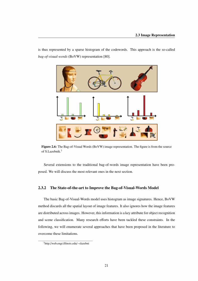
2.3 Image Representation
is thus represented by a sparse histogram of the codewords. This approach is the so-called
bag-of-visual-words (BoVW) representation [80].
Figure 2.6: The Bag-of-Visual Words (BoVW) image representation. The figure is from the sourceof S.Lazebnik.3
Several extensions to the traditional bag-of-words image representation have been pro-
posed. We will discuss the most relevant ones in the next section.
2.3.2 The State-of-the-art to Improve the Bag-of-Visual-Words Model
The basic Bag-of-Visual-Words model uses histogram as image signatures. Hence, BoVW
method discards all the spatial layout of image features. It also ignores how the image features
are distributed across images. However, this information is a key attribute for object recognition
and scene classification. Many research efforts have been tackled these constraints. In the
following, we will enumerate several approaches that have been proposed in the literature to
overcome these limitations.
3http://web.engr.illinois.edu/∼slazebni
21

2. RELATED WORK
2.3.2.1 Spatial pyramid image representation
Lazebnik [4] et al. introduced a simple yet effective extension of bag-of-features image
representation, named Spatial Pyramid Matching (SPM). The idea is first to recursively subdi-
vide the image into 2r × 2r grids at multiple resolutions, then to compute the BoW histograms
for each grid sub-block at several spatial granularities, and finally to concatenate histograms of
each grid by a formulation of pyramid match kernel:
κR(Ii, I j) = IR +
R−1∑r=0
12R−r
(Ir − Ir+1) (2.17)
=12R I
0 +
R∑r=1
12R−r+1 I
r.
The weight 12R−r allows for penalizing low resolutions of a partition, reflecting the fact that
higher levels localize the features inside smaller regions more precisely, see Figure 2.7. Using
B visual words in a visual dictionary and C grid cells in SPM will result in a histogram of size
BC as the final image representation.
Figure 2.7: An example of constructing a three-level pyramid. The image has three feature types,indicated by circles, diamonds, and crosses. At the top, the SPM method subdivides the image atthree different levels of resolution. Next, for each level of resolution and each grid cell, SPM countsthe features that fall in each spatial bin. Finally, SPM weights each spatial histogram according toEquation (2.17). The figure is excerpted from Lazebnik et al. [4].
In such a way, the spatial distribution of these visual features is encoded into the final spatial
pyramid image representation with level weighted normalizations. Despite on hypothesis of
22

2.3 Image Representation
uniform spatial layout in image, SPM does not only beat the simple BoVW by a large margin
but also performs competitively against much elaborate methods.
2.3.2.2 Superpixels
Ren et al. [17] put forward a concept of grouping pixels into “superpixels”. The aim of
superpixels is to over-segment image into a large number of coherent, local regions which
retain most of the structure necessary for segmentation at the scale of interest. See an example
in Figure 2.8. The compact superpixels can capture diverse spatially coherent information and
multi-scale visual patterns of a natural image.
(a) (b)
Figure 2.8: An example of superpixels. (a) Input image. (b) A “superpixel” map with 200 super-pixels via Normalized Cuts algorithm [5]. The figure is excerpted from Mori et al. [6].
Superpixels are often used as a preprocessing step in computer vision to reduce the com-
plexity of image analysis for later processing stages. The original superpixel algorithm used
Normalized Cuts (NCuts) based on contour and texture cues [6, 17]. Later a variety of new su-
perpixel algorithm have been developed, e.g. TurboPixels [89], Simple Linear Iterative Cluster-
ing (SLIC) superpixels [90], Superpixels Extracted via Energy-Driven Sampling (SEEDS) [91].
A shortcoming of this approach is: Superpixels are usually expected to align with object
boundaries, but this may not hold strictly in practice due to faint object boundaries and cluttered
background [92].
23
2. RELATED WORK
2.3.2.3 Using class-specific codebooks to vote for object position
Leibe et al. [13] proposed to build a class-specific codebook for the target object category.
The procedure of codebook generation works as follows. Firstly, image patches from training
images are extracted with the Harris interest point detector [28]. Secondly, these patches are
treated as individual clusters on which agglomerative clustering is performed initially. The
clustering process stops until the similarity between any patches in different clusters is less
than a certain threshold. Finally, the codebook is generated from the center of each resulting
cluster. The authors called this adapted codebook a Codebook of Local Appearance.
Leibe et al. also define an Implicit Shape Model (ISM) to model the spatial distribution of
each codebook entry under a probabilistic framework. More precisely, IS M(C) =(IC , PI,C
),
where IC is the aforementioned codebook of local appearance for a given category C, PI,C is
a spatial probability distribution for the codebook entry. PI,C estimates where the codebook
entry may be found on the object in a non-parametric manner. Hence, the class characteristics
are learnt in such a soft-coded way. We can vote for object position or even handle multiple
articulated objects of the same class in testing images.
2.3.2.4 Spatiograms versus Histograms
Histograms, as graphical representation of the data distribution, have been widely used to
describe image regions. However, all spatial information is discarded and only features occur-
rence counts are retained in such a description. Birchfield et al. [18] introduced spatiograms
as a generalization of the histograms to allow higher-order spatial moments to be part of the
descriptor. Conaire et al. [93] further proposed an improved spatiogram similarity measure that
was derived from the Bhattacharyya coefficient [94] for spatiogram comparison.
Formally, a histogram can be formulated as: Given a discrete function f : x → z, where
x ∈ X and z ∈ Z, a histogram of f is h f : z→ Z∗, where Z∗ is the set of non-negative integers.
h f (z) is the number of elements x ∈ X such that f (x) = z.
In contrast, for an image I j, its spatiograms can be expressed by rewriting the aforemen-
tioned function f as a two-dimensional mapping I j : P → z, where P = [X,Y]T is a set of
pixels of an image, [X,Y]T is a set of their corresponding coordinates in the image. Hence, the
(second-order) spatiogram of an image is denoted by:
hI j(b) = 〈nb, µb,Σb〉, b = 1, . . . , B, (2.18)
24
2.3 Image Representation
where nb is the number of pixels whose values fall into the bth bin, i.e. the set nbb=1,...,B
corresponds exactly to the histogram. The µb and Σb represent the mean vector and covariance
matrices of those pixels’ coordinates respectively. B is the number of bins in the spatiogram.
Compared with co-occurrence matrices [49], spatiograms capture the global positions of
the pixels rather than their pairwise relationships.
2.3.2.5 Spatial orientations of visual word pairs to improve Bag-of-Visual-Words model
Khan et al. [95] proposed to embed global spatial information of visual words into BoW
model through the histograms of orientations for any pairs of visual words of the same type.
The authors introduced a notation Pair of Identical visual Words (PIW), which is defined as the
set of all the pairs of visual words of the same type. A spatial distribution of visual words is
represented as a histogram of orientations of the segments formed by PIW.
2.3.2.6 Improve BoW model with respect to feature encoding
Features encoding, i.e. transforming local image descriptors into histograms is at the heart
of bag-of-visual-words model. A large number of methods have been proposed to improve
this encoding process in feature space. Recently, many efforts can be found in the literature
regarding this direction. Here we enumerate some notable approaches, such as Fisher vector
image representation [20, 21, 96–99], sparse coding [100], locality constrained linear coding
(LLC) [101], spatially local coding [102] etc. that compete with SPM to give extensions of
bag-of-words image representations to encode spatial layout.
2.3.3 Region-based Image Representation
Many works on region-based image representation (RBIR) can be found in the litera-
ture [103, 104]. We introduce several notable ones.
Stricker et al. [45] proposed to divide an image into 5 partially overlapping, fuzzy regions.
Next, they compute the first three moments of the color distribution for each region. Finally, an
image is represented by a feature vector that is composed of color moments of 5 fuzzy regions
for image indexing. That is to say, the index entry consists of 45 (number of regions × number
of color channels × three moments, i.e. 5 × 3 × 3) floating numbers per image for indexing.
Based on fuzzy regions, the feature vectors in the index achieve relatively invariance to small
translations and small rotations of an image.
25
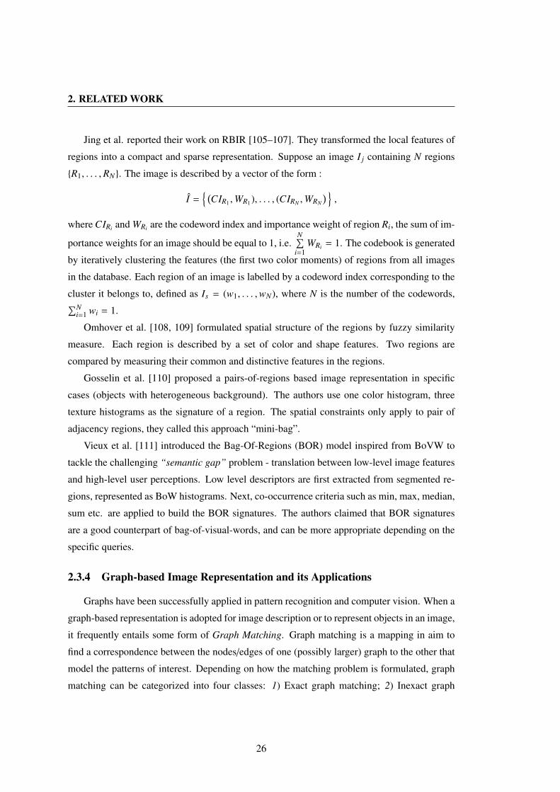
2. RELATED WORK
Jing et al. reported their work on RBIR [105–107]. They transformed the local features of
regions into a compact and sparse representation. Suppose an image I j containing N regions
R1, . . . ,RN. The image is described by a vector of the form :
I = (
CIR1 ,WR1), . . . , (CIRN ,WRN
) ,
where CIRi and WRi are the codeword index and importance weight of region Ri, the sum of im-
portance weights for an image should be equal to 1, i.e.N∑
i=1WRi = 1. The codebook is generated
by iteratively clustering the features (the first two color moments) of regions from all images
in the database. Each region of an image is labelled by a codeword index corresponding to the
cluster it belongs to, defined as Is = (w1, . . . ,wN), where N is the number of the codewords,∑Ni=1 wi = 1.
Omhover et al. [108, 109] formulated spatial structure of the regions by fuzzy similarity
measure. Each region is described by a set of color and shape features. Two regions are
compared by measuring their common and distinctive features in the regions.
Gosselin et al. [110] proposed a pairs-of-regions based image representation in specific
cases (objects with heterogeneous background). The authors use one color histogram, three
texture histograms as the signature of a region. The spatial constraints only apply to pair of
adjacency regions, they called this approach “mini-bag”.
Vieux et al. [111] introduced the Bag-Of-Regions (BOR) model inspired from BoVW to
tackle the challenging “semantic gap” problem - translation between low-level image features
and high-level user perceptions. Low level descriptors are first extracted from segmented re-
gions, represented as BoW histograms. Next, co-occurrence criteria such as min, max, median,
sum etc. are applied to build the BOR signatures. The authors claimed that BOR signatures
are a good counterpart of bag-of-visual-words, and can be more appropriate depending on the
specific queries.
2.3.4 Graph-based Image Representation and its Applications
Graphs have been successfully applied in pattern recognition and computer vision. When a
graph-based representation is adopted for image description or to represent objects in an image,
it frequently entails some form of Graph Matching. Graph matching is a mapping in aim to
find a correspondence between the nodes/edges of one (possibly larger) graph to the other that
model the patterns of interest. Depending on how the matching problem is formulated, graph
matching can be categorized into four classes: 1) Exact graph matching; 2) Inexact graph
26

2.4 Conclusion
matching; 3) Graph embeddings and graph kernels; 4) Other graph matching techniques. The
first category and the second one are respectively restricted to strict and more or less difference
in the structure of the graphs being matched. The third one are the techniques actually gaining
a growing interest in recent literature [22–24, 112, 113]. In this manuscript, we only cite one
instance: Graph Words, which has highly motivated our present work.
Graph Words Karaman proposed a graph-based image representation via “Graph Words” [7].
The idea of the method consists in building a set of “small” graphs on multiple nested layers,
and then in fitting these graph features to bag-of-visual-words approach, as demonstrated in
Figure 2.9. The author defined a maximum of four layers of Graphs Words due to high compu-
tational cost of the approach. From bottom to top, the first layer contains only a fixed number
of seeds points which are positioned at salient SURF points with higher response [35]. The
second to fourth layer correspond respectively to graphs with 3,6 and 9 nearest neighbours
of the seeds. Graph edges are generated by Delaunay triangulation on each layer separately.
Under such definition, the number of graphs at each layer is the same. Graph comparison can
be achieved by Context Dependent Kernel (CDK) [114]. In contrast to traditional visual dic-
tionary, each codeword is defined as the median graph that minimizes the distance to all the
graphs of the corresponding cluster. The spatial layout is therefore embedded at feature level
in such multi-resolution of graph structure.
2.4 Conclusion
In this Chapter, we have presented image descriptors, image representation and image re-
trieval in real world, particularly Content-Based Image Retrieval (CBIR). With respect to image
representation, we mainly focus on the bag-of-visual-words model and its variants. One of se-
vere limitations of the bag-of-visual-words model is that it ignores the spatial layouts among
the image patches, which are very important information in image representation. Several ef-
fective methods have been proposed to incorporate the spatial information into BoVW. We
enumerated a few of notable ones. In the present work, we are especially interested in using
graphs as a tool to model spatial relationships among image features. This idea has motivated
our direction in the next Chapter.
27

2. RELATED WORK
Figure 2.9: A hierarchy of “nested” Graph Words on four layers (on the left) in the same exampleof image (on the right). Seed is marked as hollow circle in white color, and neighbour nodes areshown as solid circles in black color. The figures are extracted from [7].
28
Chapter 3
Graph-based Image Representation
As discussed in Chapter 2, graphs are powerful tools to model spatial information in image
representation. Graph-based representations are of pivotal importance in computer vision and
pattern recognition [115]. Describing the image patterns with such representations is quite
natural and find applications in both low level image processing and high level vision tasks.
The patterns and objects in images are identified by decomposing the image into parts and
analysing the relationships/structure between them.
In this Chapter, we first introduce the image graph model. Next, we explain how this pro-
posed model is described by a weighted image graph. The weighted image graph is composed
of graph nodes, edges and the corresponding edge weights. An edge weight measures the simi-
larity between two nodes of the edge. Then we discuss the weighted graph construction process
step by step. Different objective functions for edge weights are designed. Finally, three graph
partitioning methods are presented for dividing the image graph into a series of subgraphs.
These subgraphs is then used as image descriptors embedding the color/texture homogeneity
and limited spatial information of the image.
3.1 An Overview of the Image Graph Model
Let us first introduce the key components and concepts of the image graph model for image
retrieval. The processing chain for image graph model includes the following steps: 1) graph
construction; 2) graph partitioning; 3) (sub)graph matching; 4) image retrieval. See Figure 3.1.
29

3. GRAPH-BASED IMAGE REPRESENTATION
Figure 3.1: An overview of the processing chain for the proposed image graph model. (I)Image is represented by an initial weighted graph. (II) Graph partitioning consists in finding theoptimal labeling for each graph nodes. (III) Find the best bipartite matched subgraphs betweenimages pairs (IV) Retrieve images based on signatures that define the similarities between thesesubgraphs.
3.2 Weighted Image Graph Representation
Intuitively, a graph represents a set of elements and a set of pairwise relationships between
these elements. The elements are called nodes or vertices, and the pairwise relationships
between the nodes are called edges.
A graph G = (V, E) is represented by a set of vertices V and a collection of edges E ⊆ V×V .
Each edge connects a pair of vertices. If all edges in a graph have no orientation, i.e., the
edge (a, b) is identical to the edge (b, a), then this graph is called undirected graph. An edge-
weighted graph (or for short, weighted graph), is defined as a pair (G,w) in which w(e) : e→ R
is a weight function mapping each edge e ∈ E to its weight. Weighted graphs, as a model, are
used in numerous problems, such as networks where graph nodes are linked with different
weights (distance, cost, etc.). Note that a graph can be viewed as an edge-weighted graph
where all edges have a weight equalling to 1.
An input image database Ω, is composed of N RGB images Ω = I1, . . . , IN. We define
G j = (V j, E j,W j) as the undirected weighted image graph constructed on the image I j. The set
of vertices V j contains a subset of pixels P of the image I j and at the limit can contain all of
them. The graph edges E j connect these vertices with a specified neighbourhood system. W j
is an affinity matrix of size |V j| × |V j|, whose entry at row p, and column q is Wpq, defined as:
Wpq =
wpq if p, q ∈ E j
0 if p, q < E j,(3.1)
where wpq represents the edge-based similarity between two vertices p and q.
30

3.3 Graph Construction
3.3 Graph Construction
With the above notation, we can now define the graph nodes (vertices), graph edges and
graph weights in image graph.
3.3.1 Graph Nodes Selection in Image Graph
We experimented two methods for nodes selection. We describe them in the following.
3.3.1.1 Prominent keypoints
Feature extraction First, a feature-extraction algorithm is used to extract the feature points
either on the whole image or on the mask of the object being retrieved. An example can be
seen in Figure 3.2(a), where the SURF points [35] are chosen in our experiments. A threshold
(Thrh) on the Hessian of the SURF descriptors is set. The larger the threshold value, the less
keypoints are selected. A good value for Thrh could be from 300 to 500, depending from the
image contrast. By default, the value of Thrh is set to 400.
Key points filtering Next, all the extracted feature points are further sorted by their feature
strengths. In such a way, the most strong/prominent key points with the most representative
features remain. In some cases, the extracted points may be very close to each other, which
leads to unbalanced graph edges. To avoid that, we filter the feature points by preserving only
the most prominent key point over any 10-pixels diametrical region. After filtration, we obtain
a set of reduced keypoints P = p1, ..., pn, see Figure 3.2(b). However, graph nodes obtained
in such a way are very sparse and irregular in either the number of nodes or the distances in
between, losing interesting information potentially.
3.3.1.2 Dense sampling strategy
First image pixels are chosen by dense sampling the points at a fixed spacing on a regular
grid. Next, the local SIFT features [2] of these points are extracted from their image patches.
We call this approach Bag-of-Features Grid SIFT (BF-GSIFT) [36].
This sampling approach gives a constant amount of features per image area since all patches
with strong or less contrast contribute equally to the overall image representation. In contrast
to the previous strategy, i.e. prominent keypoints selection, that has more arbitrary spatial
relations between features, dense sampling keeps simple spatial relations between features in
31

3. GRAPH-BASED IMAGE REPRESENTATION
(a) (b) (c)
(d) (e) (f)Figure 3.2: Graph construction. (a) Initial SURF keypoints. (b) Filtered keypoints. (c) Seedsselection. (d) Delaunay triangulation over filtered feature points. (e) Graph-cuts result. (f) Labelingresult.
reserve by following a regular pattern. On the downside, dense sampling cannot reach the same
level of repeatability as obtained with interest points unless sampling is performed extremely
densely but then the number of features quickly grows unacceptably large. In practice, re-
searchers often use an overlap between patches of 50% or less. As in SPM [4], we adopt
8-pixels spacing, 16-pixels patch size, to reach a compromise between repeatability of interest
points and reasonable size of features.
3.3.2 Graph Edges Construction in Image Graph
Once vertices are fixed, we adopt a suitable neighbourhood system to generate graph edges
based on the strategy of nodes selection. The purpose is to keep the spatial structure between
local features so that it is invariant to image translation, scaling, and rotation.
32

3.3 Graph Construction
In general, there are three options for graph edges construction: 1) Delaunay Triangulation,
2) 4-neighbourhood, 3) 8-neighbourhood.
(a) Delaunay triangulation (b) 4-neighbourhood (c) 8-neighbourhood
Figure 3.3: Options for the neighbourhood system of image graph.
In the context of prominent keypoints, a Delaunay triangulation (DT) [116] is performed
over all filtered points set P to generate the edges of image graph. The DT process aims to
maximize the minimum angle of all triangles’ angles. Therefore, it avoids skinny triangles
between edges. More precisely, the Delaunay triangulation of a point set is a collection of
edges satisfying an “empty circle” property: For each edge we can find a circle containing the
edge’s endpoints but not containing any other points. This kind of triangulation is equivalent
to the nerve of the cells in a Voronoi diagram. An example of Delaunay triangulation on top
of the Voronoi diagram (in dotted lines) can be seen in Figure 3.3(a). Another example of DT
over the vertices of an image graph is shown in Figure 3.2(d). This technique is used for the
prominent keypoints approach.
For the dense sampling approach, a regular d-neighbourhood (d = 4 or d = 8) system
is used. The 4-neighbourhood of vertice p are the four pixels to the north (p2), south (p6),
east (p4), and west (p8), see Figure 3.3(b). The 8-neighbourhood of node p also includes the
diagonals, namely pixels p1, . . . , p8, see Figure 3.3(c).
3.3.3 Graph Weights in Image Graph
Following the aforementioned definitions, let us suppose that the graph edges E connect the
vertices with a predefined neighbourhood system. The edge affinity matrix W of size |V | × |V |,
is assumed to be non-negative and symmetric.
As discussed in Section 2.1.6, color and texture are two predominant factors to characterize
the image features. Therefore, in the present work, we design an edge-weight function that
combines joint color-texture features. For an edge between two nodes p and q, its weight is
33

3. GRAPH-BASED IMAGE REPRESENTATION
defined as follows:
wpq = e−λ·α·CpqΣ−1C CT
pq · e−λ·(1−α)·TpqΣ−1T T T
pq
=(wC
pq
)α·(wT
pq
)1−α. (3.2)
where wCpq is a color-related weight term, and wT
pq is a texture-related weight term. The param-
eterα controls the relative impact of local color and texture patterns on the edge weights of the
graph and can be adjusted in the optimization process. Edge weights 1) only take color infor-
mation into account if α = 1; 2) factor color out, considering texture only if α = 0; 3) combine
color and texture features if 0 < α < 1.
We adopt the positive definite Gaussian function in Equation (E.1), due to its good property
that has been proved in the literature [5, 117–119]. In the next two Subsections, we elaborate
the color term and texture term respectively.
3.3.3.1 Color weight
Color Space Selection A color space is used to specify a three-dimensional color coordinate
system and a subspace of the system in which colors are represented as three points [75]. In the
present work, we finally decide to adopt YUV color space instead of RGB color space [120],
for the following reasons:
YUV color space has independent color channels, in terms of one luma (Y’) and two
chrominance (UV) components. Moreover, there are couples of main disadvantages [121] with
the RGB color space: 1) It is not independent, has redundant information in color channels;
2) The RGB color space is not perceptually uniform; 3) All components (R,G, B) have equal
importance and, therefore, these values have to be quantized with the same precision.
Given an input color image, we first decorrelate the RGB fields into the YUV color space
by Equation (3.3). The Y stands for the luma component (the brightness) and U and V are the
chrominance (color) components. We use the YUV color space, since it has independent color
channels and allows to better deal with illumination changes.
Y = 0.299R + 0.587G + 0.114B (3.3a)
U = (B − Y) ∗ 0.565 (3.3b)
V = (R − Y) ∗ 0.713 (3.3c)
34
3.3 Graph Construction
The color weights on the edges are defined as:
wCpq = e−λ·CpqΣ−1
C CTpq = e−λ·(Cp−Cq)Σ−1
C (Cp−Cq)T, (3.4)
where Cpq = Cp − Cq, Cp = (Yp, Up, Vp) and Cq = (Yq, Uq, Vq) account for the mean color
vector over a n × n patch centred on points p and q respectively in YUV color space. In our
experiments, these two vectors are each computed over a 5× 5 region in 4-neighbourhood
system centred on p and q. As the aforementioned discussion, we use the YUV color space in
order to have independent color channels.
We denote Yp = Y(x, y), respectively Up = U(x, y) and Vp = V(x, y), as the color channel
values at point p = (x, y) in the coordinate system of the whole image. The mean color vector
reads Cp = (Yp, Up, Vp) where:
Yp =1n2
n∑u=−n
n∑v=−n
Y(x + u, y + v) ,
Up =1n2
n∑u=−n
n∑v=−n
U(x + u, y + v) ,
and
Vp =1n2
n∑u=−n
n∑v=−n
V(x + u, y + v) .
The covariance matrix
ΣC =
σ2
Y 0 00 σ2
U 00 0 σ2
V
is computed from, for all three channels, the mean of the mean color vector of all nodes.Moreover, the covariance matrix Σc is considered diagonal because of channels’ independence.As in [122], the covariance is defined for each channel as:
σ2Y =
⟨(Yp − Yq
)2⟩
σ2U =
⟨(Up − Uq
)2⟩
σ2V =
⟨(Vp − Vq
)2⟩
where 〈.〉 denotes the expectation over all the edges (p, q) ∈ E of the image graph G.
35

3. GRAPH-BASED IMAGE REPRESENTATION
Figure 3.4: Block DCT on 8 × 8 pixel patch.
Figure 3.5: A block of 8×8 pixel on DCT, the soliddot in black denotes thegraph node, the 64 DCTcoefficients are scanned ina “zig-zag” fashion.
3.3.3.2 Texture weight
Texture based on DCT Given an image graph, the 2D block DCT-based transform is pro-
cessed on 8×8 blocks of pixels around each graph node with level shift. As shown in Figure 3.4,
each block contains one DC coefficient (in green) and 63 other AC coefficients (in red). The
DC coefficient represents the average intensity value of the patch, and carries most of the en-
ergy and the perceptual information. The AC coefficients contain frequency information. The
position of graph node within the block is shown in Figure 3.5.
The texture-related weight term wTpq based on DCT is defined as:
wTpq = e−λ·TpqΣ−1
T T Tpq = e−λ·(Tp−Tq)Σ−1
T (Tp−Tq)T(3.5)
where Tpq = Tp −Tq, Tp is a row vector composed of k low frequency AC coefficients in 8× 8
DCT block centred on point p. Tq is defined similarly. The covariance ΣT is computed over
DCT blocks for each coefficient independently over each node in G.
The vector Tp has the following variants depending on the number of coefficients and the
channel(s) in the YUV color system from which these coefficients are extract: 1) five low fre-
quency coefficients in luma (Y) component (Equation (3.6)), its corresponding covariance is
defined in Equation (3.7), see Figure 3.6; 2) ten low frequency coefficients in luma (Y) compo-
nent (Equation (3.8)); 3) five low frequency coefficients in luma (Y) component, plus two low
frequency coefficients in chrominance components (U and V) respectively (Equation (3.9)).
36

3.4 Graph Partitioning
Tp =(dY (1, 0) , dY (0, 1) , dY (0, 2) , dY (1, 1) , dY (2, 0)
)(3.6)
ΣT = diag[σ2d(1,0), σ
2d(0,1), σ
2d(0,2), σ
2d(1,1), σ
2d(2,0)] (3.7)
Tp =(dY (1, 0), dY (0, 1), dY (0, 2), dY (1, 1), dY (2, 0), dY (3, 0), dY (2, 1), dY (1, 2), dY (0, 3)
)(3.8)
Tp =(dY (1, 0), dY (0, 1), dY (0, 2), dY (1, 1), dY (2, 0), dU(1, 0), dU(0, 1), dV (1, 0), dV (0, 1)
)(3.9)
Figure 3.6: The DCT (Discrete Cosine Transform) block is scanned in a diagonal zigzag patternstarting at the DC coefficient d(0,0) to produce a list of quantized coefficient values. Here only fiveAC coefficients d(1,0), d(0,1), d(0,2), d(1,1), d(2,0) in luma (Y’) component of YUV system areconsidered due to their good discriminative properties.
3.4 Graph Partitioning
After that the weighted image graph has been built, we can now shift our focus to the
problem of graph partitioning. Graph partitioning is also called graph clustering. In this
model of clustering, we are given an image graph G j for each image I j in the database. We
seek to partition the graph G j into fixed K disjoint unconnected subgraphs g j,1, . . . , g j,K,
such that ∀k , l, g j,k∩g j,l = ∅ and G j = ⋃K
k=1 g j,k∪E j, where E j ⊂ E j are the removed edges
to divide G j by graph cuttings. The partitioning divides vertices V j into a set of the vertices
v j,1, . . . , v j,K in the corresponding subgraphs, such that v j,m ∩ v j,n = ∅ for m , n. We denote
this K-way partitioning [123] by ΓKj = Γk
jk=1, ..., K = g j,1, . . . , g j,K.
37

3. GRAPH-BASED IMAGE REPRESENTATION
3.4.1 Graph-based Image Segmentation Problem
Graph partitioning can be considered as a graph-based image segmentation problem as
well [124]. The idea of graph-based image segmentation is that the set of points are represented
as a weighted undirected graph G = (V, E, W), where a set of vertices (nodes) V represents
the points in the image. E is a set of edges connecting the nodes. W is an affinity matrix of
size |V | × |V |, whose entries are the weights of the edges. An entry of W is zero if there is no
edge between the corresponding vertices. The weight on each edge W(i, j) is a function of the
similarity between the nodes i and j. The graph G is segmented into K disjoint sets by cutting
the edges connecting these K parts. The degree of similarity between any two parts is the total
weights of the edges that separate them.
3.4.2 Image Graph Labeling Problem
Graph partitioning can also be considered as a labeling problem. Given a set of vertices V
and a finite set of labels L = 1, 2, . . . ,K, for any node p ∈ V , we are looking for the optimal
label lp ∈ L, such that the joint labeling L = l1, . . . , l|V | ∈ L|V | satisfies a specified objective
function. Reciprocally, an optimal labeling L on the image graph can be represented by an
optimal partition P of graph nodes, where P = Pl | l ∈ L, and Pl = p ∈ P | lp = l is a subset
of graph nodes assigned label l. Obviously, there is a bijective function (mapping) between
partition P and labeling L.
Energy minimization Many computer vision problems, including labeling problem can be
formulated in terms of energy minimization. For the image graph G = (V, E), the energy
function contains two terms:
J(L) =∑p∈V
fp(lp) +∑
(p,q)∈E
fpq(lp, lq) . (3.10)
lp denotes the label of graph node p ∈ V that must belong to a finite label set L. The unary
terms fp(·) encode the data penalty functions, and the pairwise terms fpq(· , ·) are interaction
potentials.
This energy (Equation (3.10)) is often derived in the context of Markov Random Fields
(MRF) [50, 51]: a minimum of energy J(L) corresponds to a maximum a-posteriori (MAP)
labeling L.
38

3.5 Graph Partitioning Approaches
3.5 Graph Partitioning Approaches
In this Section, we review three graph partitioning methods, namely, Graph Cuts, Normal-
ized Cuts and kernel k-means. As you will see in the next Chapters, we use and compare these
three approaches within our system for image retrieval.
3.5.1 Graph Cuts: energy-based method
The Graph Cut [8, 9, 125, 126] is a semi-supervised method based on min-cut/max-flow
algorithms from combinatorial optimization. This technique can be used to find the global
minimum of some multi-dimensional energy functions. The formulation of Graph Cuts can be
either perceived from graph partition point of view (Section 3.5.1.1), or regarded as an energy
minimization on a graph from energy point of view (Section 3.5.1.3).
3.5.1.1 Binary labeling
In the context of Graph Cuts, the weighted graph G = (V, E) has two distinguished vertices
called the terminals. One of the terminals s ∈ V is called the source and the other one t ∈
V is called the sink. A cut C ⊂ E is a set of edges such that the terminals are separated
in the induced graph G(C) = (V, E − C). In addition, no proper subset of C separates the
terminals in G(C). The cost of the cut C, denoted |C|, equals the sum of its edge weights.
The minimum cut problem on a graph is to find a cut with the smallest cost among all cuts.
There are a large number of fast algorithms for this problem in the binary labeling case. For
example, in combinatorial optimization domain, the minimum s/t cut problem can be solved
in polynomial time by finding a maximum flow from the source s to the sink t. This is the so-
called max-flow/min-cut algorithm. In practice, the algorithm is based on the Ford-Fulkerson
algorithm [127]. An example is shown in Figure 3.7.
Main idea for Min-cut/Max-flow methods Before introducing the min-cut/max-flow prob-
lem, let us give the following definition.
Definition 1. Flow network A flow network is defined as a directed graph where an edge hasa non-negative capacity. For an edge (p, q) ∈ E, its capacity is denoted by c(p, q).
39
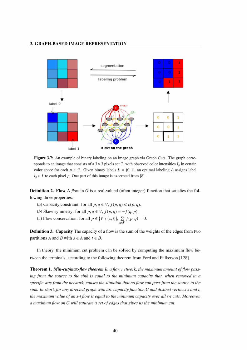
3. GRAPH-BASED IMAGE REPRESENTATION
Figure 3.7: An example of binary labeling on an image graph via Graph Cuts. The graph corre-sponds to an image that consists of a 3× 3 pixels set P, with observed color intensities Ip in certaincolor space for each p ∈ P. Given binary labels L = 0, 1, an optimal labeling L assigns labellp ∈ L to each pixel p. One part of this image is excerpted from [8].
Definition 2. Flow A flow in G is a real-valued (often integer) function that satisfies the fol-lowing three properties:
(a) Capacity constraint: for all p, q ∈ V , f (p, q) 6 c(p, q).
(b) Skew symmetry: for all p, q ∈ V , f (p, q) = − f (q, p).
(c) Flow conservation: for all p ∈V \ s, t
,∑
q∈Vf (p, q) = 0.
Definition 3. Capacity The capacity of a flow is the sum of the weights of the edges from twopartitions A and B with s ∈ A and t ∈ B.
In theory, the minimum cut problem can be solved by computing the maximum flow be-
tween the terminals, according to the following theorem from Ford and Fulkerson [128].
Theorem 1. Min-cut/max-flow theorem In a flow network, the maximum amount of flow pass-ing from the source to the sink is equal to the minimum capacity that, when removed in aspecific way from the network, causes the situation that no flow can pass from the source to thesink. In short, for any directed graph with arc capacity function C and distinct vertices s and t,the maximum value of an s-t flow is equal to the minimum capacity over all s-t cuts. Moreover,a maximum flow on G will saturate a set of edges that gives us the minimum cut.
40

3.5 Graph Partitioning Approaches
From this theorem, an algorithm has been proposed. It requires two following definitions
to understand it.
Definition 4. Augmenting path A path from the source s to the sink t that can deliver anincreased flow is called a flow augmenting path.
Definition 5. Residual Graph of a flow network is a graph which indicates additional possibleflow. If there is a path from the source to the sink in a residual graph, then it is possible to addflow. Every edge of a residual graph has a value called residual capacity which is equal tooriginal capacity of the edge minus current flow. Residual capacity is basically the currentcapacity of the edge.
The min-cut/max-flow algorithm can now be given: The minimum cut edges can be ob-
Algorithm 1 Max-flow/Min-cut AlgorithmRequire: Graph G = (V, E), source s, terminal t, capacity CEnsure: Return f as the Max-flow, and (X,V − X) as the Min-cut
1: set P← 0 (flow 0 on all edges), set opt ← f alse2: while not opt do3: Construct the residual graph G f
4: Find a directed path P from s to t in G f (an augmenting path)5: if such an augmenting path P exists then6: Update flow f along P7: else8: set opt ← true9: set X the set of vertices in G f reachable from s
10: end if11: end while
tained by the following steps: 1) Run Ford-Fulkerson Algorithm 1 and consider the final resid-
ual graph. 2) Find the set of vertices that are reachable from the source in the residual graph.
3) All edges which are from a reachable vertex to a non-reachable vertex are minimum cut
edges.
3.5.1.2 Extension to multi-label problems
The weighted graph G = (V, E) may involve more than two terminals. The multi-labeling
problem can be considered as the generalization of the minimum s/t cut problem. An exam-
41

3. GRAPH-BASED IMAGE REPRESENTATION
ple is the multi-way cut. The problem becomes NP-hard even in the simplest discontinuity-
preserving case. Therefore, some approximate methods such as α-β swap and α-expansion [8,
9] are often used.
Definition 6. α-β swap Given a pair of labels α, β, a move from a partition P (labeling L) to anew partition P ′ (labeling L′) is called an α-β swap if Pl = P′l for any label l , α, β.
Definition 7. α-expansion Given a label α, a move from a partition P (labeling L) to a newpartitionP ′ (labeling L′) is called an α-expansion if Pα ⊂ P′α and P′l ⊂ Pl for any label l , α.
(a) (b) (c)
Figure 3.8: Example of α-β swap and α-expansion. (a) initial labeling: α in red, β in green, γin blue. (b) α-β swap: only number of pixels with label α or β change their labels, pixels withlabel γ remain unchanged. (c) α-expansion: pixels with different labels can change their labelssimultaneously. The figures are excerpted from [9]. This figure is better viewed in color.
3.5.1.3 Graph Cuts from perspective of energy minimization
In the present work, the Graph Cut is used to minimize energy functions of two terms:
J(L) = Jdata(L) + Jsmooth(L)
=∑p∈V
Jd(p, lp) +∑
(p,q)∈E
Js(p, q)
=∑p∈S
Jd(lp) +∑
(p,q)∈E
Js(p, q) . (3.11)
Jdata(L) is the data term. In our case, it is only applied to user-defined hard constraints (seeds
here) imposed on the initialization of Graph Cuts. We denote a set of seed points by S =
s1, . . . sK, where K is the predefined number of subgraphs obtained after graph partitioning.
The seeds are placed on the image before running the Graph Cuts algorithm.
42

3.5 Graph Partitioning Approaches
The goal of the data term is to fix the label of the seed points. For instance, the seed pointsi must end up with label i after the energy minimization process. This idea can be formulatedas in [9]:
Jd(lp) =
0 if p = si & lp = i∞ otherwise.
(3.12)
As for the smoothness term Jsmooth(L), this term measures the discontinuity between node p
and its neighboring pixels. The use of α-expansion imposes three constraints on the smoothing
term Jsmooth, see Equation (3.11):
1. Jsmooth(α, β) = 0⇔ α = β or Jsmooth(α, β) , 0⇔ α , β
2. Jsmooth(α, β) = Jsmooth(β, α) ≥ 0
3. Jsmooth(α, β) ≤ Jsmooth(α, γ) + Jsmooth(γ, β)
The first two terms tell that an energy between two different labels α and β should be non-zero.
If it is zero, then two labels are the same. The last term defines the triangle rule. A short cut
is always cheaper or similar than taking the whole path. If the smoothness term only satisfies
the first two terms, it is called a semi-metric term. If the last term is also satisfied, it is said a
metric term. The α-expansion algorithm can only be used with metric terms. Otherwise, the
alpha-beta swap can be used with semi-metric or metric terms. Note that in Equation (3.11),
Jsmooth(L) satisfies the metric term.
To follow the pre-stated requirements, we will encourage that any two neighbouring nodes
(p, q) ∈ E are 1) spatially close to each other; 2) if node p and q have similar colors, they tend
to have the same label.
Jsmooth(L) is directly linked to wpq, the edge weights of the image graph. The wpq is
defined as in Equation (E.1). In the present work, we propose the following variant definitions
for Jsmooth(L):
Js(p, q) = wpq(1 − δ(lp, lq)
), (3.13)
or
Js(p, q) =wpq
‖p − q‖2(1 − δ(lp, lq)
), (3.14)
or
Js(p, q) = wpq fd(p, q)(1 − δ(`p, `q)) , (3.15)
43

3. GRAPH-BASED IMAGE REPRESENTATION
where δ(`p, `q) is the Kronecker’s delta:
δ(`p, `q) =
0, if `p , `q
1, if `p = `q .(3.16)
In Equation (3.15), the distance between nodes is introduced via fd(p, q). This distance term
fd(p, q) is defined as:
fd(p, q) = exp(−λ2(p − q)Σ−1
d (p − q)T). (3.17)
The matrix Σd is also considered diagonal. Let us denote d(p, q) as the L2 distance between the
node p and q. The d(p, q) =
√(xp − xq)2 + (yp − yq)2. We propose several definitions for Σd
as follows:1)
Σd =
dE(p, q) 00 dE(p, q)
, (3.18)
where dE(p, q) is the mean distance of all neighbouring points in the graph G, i.e.
∀(p, q) ∈ E, dE(p, q) =
∑(p,q)∈E
d(p, q)
|E|
=
∑(p,q)∈E
√(xp − xq)2 + (yp − yq)2
|E|. (3.19)
2)
Σd =
∑(p,q)∈E
(d(p, q) − dE(p, q)
)|E|
. (3.20)
3)
Σd =
∑(p,q)∈E
((d(p, q) − dE(p, q)
)· Pr(E)
)|E|
, (3.21)
where Pr(E) is the probability of the distance of an edge falls into the bin that d(p, q) belongs
to. In our experiments, we set the number of bin size to 10.
Among the above three options for the distance term, the Equation (3.18) is easier to com-
pute and has been proven to achieve better graph cuts result. However, we have also observed
that embedding distance factor fd(p, q) in the smoothness term does not give any improvement
to partition results; in the case of sparse sampling, it is even worse. Therefore, we decide that
fd(p, q) can be factored out of the equations. In our case, we use Equation (3.13), i.e., we only
consider color and (or) texture factor(s) in the smoothness term in the following discussion.
44

3.5 Graph Partitioning Approaches
3.5.1.4 Seed selection
1) In the case of prominent keypoints approach: to ensure that seeds with different labels will
fall into heterogeneous regions in the image, we select seeds in such a way:
a) The fixed number of seed points S ⊂ P are chosen among the most prominent keypoints
in P; b) Different seeds should not be too close to each other and they should fall into
heterogeneous region of their own in the image. To achieve this purpose, we set empirically
both color and distance threshold to differentiate one seed from the other chosen ones.
For the ith seed point pi ∈ S, the data term is defined as:
D(pi, `) =
0 if ` = `i
∞ otherwise.(3.22)
An example is shown in Figure 3.2(c).
2) In the context of dense sampling: The seed points are chosen from nodes that are the closest
to the barycentre of each regular cell, see Figure 3.9.
More complex seeds selection measures (such as, choosing interest points that have the
most strong response; separating different seeds with enough distance based on image size or
resolution) have been investigated, without improving the performance.
Figure 3.9: Seed points are in hollow circle of different colors. The graph nodes are in red solidpoints.
3.5.1.5 Weakness
Due to the uncontrolled nature of the images available, automatically and precisely se-
lecting seeds from image is still beyond the reach of the state-of-the-art in computer vision.
45

3. GRAPH-BASED IMAGE REPRESENTATION
More precisely, if the seed points are manually selected, then the high level of user interac-
tion makes the Graph Cuts method useless; if the seeds are automatically selected, then the k
seed points will be highly dependent on the relationship between the background and the in-
terest object. Hence, in prominent keypoints approach, we applied a mask on the image before
running Graph Cuts to generate graph features. Unfortunately, the obtained seeds were still
not stable. An shown in Figure 3.10, three seeds between two images “fluor5Banana095” and
“fluor5Banana097” are relatively stable. In contrast, all three seeds in image “fluor5Banana098”
have fallen into background. Moreover, two of these seeds are not matched with these ones in
other two images.
fluor
5Ban
ana0
95flu
or5B
anan
a097
fluor
5Ban
ana0
98
Seeds Labeling results
Figure 3.10: Examples of seeds selection in prominent keypoints approach. The stability of seedsis hardly reached due to the uncontrolled nature of the images available. All examples of imagesare from SIVAL dataset [10]. There are three seeds in each image, and these seeds are labelled withtheir own colors (in red, orange and yellow). This figure is better viewed in color.
46

3.5 Graph Partitioning Approaches
3.5.1.6 Graph Cuts in applications
The Graph Cuts based methods have wide applications in computer vision community, such
as clustering (image segmentation) [129], image labeling [130, 131], image restoration [9, 132],
multicamera scene reconstruction [8], registration [133, 134], object tracking [135], interactive
seeded segmentation [122, 125], reducing metrication errors, filtering, stereo matching [8],
recovering the deformation map etc.
3.5.2 Normalized Cuts
As a spectral clustering technique, Normalized Cuts (NCuts) [5], is an unsupervised method
based on two graph-theoretic criteria: maximize the total dissimilarity between different sub-
graphs as well as the similarity within each subgraph. Its principle is to find a minimal cut
which is a combination of edges having minimal sum of edge values (i.e. find the least alike
pairs of nodes). Removing these edges divides the graph G j into unconnected subgraphs, such
that the similarity between nodes within a subgraph is greater than the similarity between nodes
in separated subgraphs. The advantage of the normalized cut method is that it considers two
aspects of graph segmentation: minimal cut (i.e. better separation) and preferring segments of
large size.
3.5.2.1 Basic concepts and theory
The set of points in an arbitrary feature space can be represented as a weighted undirected
graph G = (V, E), where the nodes of the graph are the points in the feature space and an edge
is formed between every pair of nodes. The weight on each edge, wi j, represents the similarity
between nodes i and j.
A graph can be partitioned into two disjoint sets A and B, with A∩B = V and A∪B = ∅,
by removing edges connecting the two parts.
Definition 8. Link Let us denote links(A,B) to be the sum of the edge weights between nodesin two disjoint sets A and B.
links(A,B) =∑
p∈A,q∈B
wpq . (3.23)
Definition 9. Degree We furthermore define the degree of A as the links of nodes in A to allthe vertices in the graph G, that is, degree(A) = links(A,V).
47

3. GRAPH-BASED IMAGE REPRESENTATION
Definition 10. Association The association (sum of all the weights) within the cluster A isdenoted by
assoc(A,A) =∑
p∈A,q∈A
wpq . (3.24)
Definition 11. Cut The degree of dissimilarity between A and B can be measured by cut(A,B),which is defined as the sum of all the weights being cut,
cut(A,B) =∑
p∈A,q∈B
wpq . (3.25)
Using a minimum cut as a segmentation criterion does not result in reasonable clusters,
since the smallest cuts usually involve isolating a single pixel. Instead of using the value of total
edge weight connecting the two partitions, Shi et al. [5] proposed a disassociation measure to
compute the cut cost as a fraction of the total edge connections to all the nodes in the graph. It
is called the Normalized Cut (NCut). The Normalized Cut examines the affinities (similarities)
between nearby pixels and tries to separate groups that are connected by weak affinities.
Definition 12. Normalized Cut (NCut) The disassociation criterion for normalized cut of Aand B is given by
NCut(A,B) =cut(A,B)
assoc(A,V)+
cut(A,B)assoc(B,V)
, (3.26)
where assoc(A,V) = assoc(A,A) + cut(A,B) =∑
p∈A,q∈Vw(p, q) is the total connection from
nodes in A to all nodes in the graph and assoc(B,V) is similarly defined.
Definition 13. Normalized association (Nassoc) The normalized association can be definedas
Nassoc(A,B) =assoc(A,A)assoc(A,V)
+assoc(B,B)assoc(B,V)
, (3.27)
where assoc(A,A) and assoc(B,B) are total weights of edges connecting nodes within A andB respectively.
Shi et al. [5] have proven that minimizing the disassociation (Equation (3.26)) is equiv-
alent to maximizing the association (Equation (3.27)) within the groups according to Equa-
tion (3.28)).
NCut(A,B) = 2 − Nassoc(A,B) . (3.28)
The two equivalent objective functions above can also be interpreted as seeking to minimize the
cut relative to the degree of a cluster instead of its size. Hence, the objectives in Equation (3.26)
48

3.5 Graph Partitioning Approaches
and Equation (3.27) can be expressed as Equation (3.29) and Equation (3.30) respectively, as
follows:
minA,B( links(A,B)
degree(A)+
links(B,A)degree(B)
)(3.29)
maxA,B( links(A,A)
degree(A)+
links(B,B)degree(B)
)(3.30)
3.5.2.2 Computing NCut by eigen-value decomposition
Unfortunately, computing the optimal NCut is NP-complete. Instead, Shi et al. suggested
solving NCuts as a regular eigenvalue problem by computing a real-valued assignment of nodes
to groups. Let x be an indicator vector of |V | dimension, where xp = 1 if node p is in A and
xp = −1 otherwise. W is an |V | × |V | symmetrical matrix with W(p, q) = wpq. l = 1, . . . , 1ᵀ
is an |V | × 1 vector of all ones. Let d = Wl be the row sums of the symmetrical matrix W,
d(p) =∑
q wpq, be the total connection from node p to all other nodes, and D = diag(d) is the
corresponding |V | × |V | diagonal matrix with d on its diagonal, Dpp =|V |∑
q=1wpq.
With the above notations, Shi et al. [5] have proved that minimizing the Normalized Cut
over all possible indicator vectors x is equivalent to minimizing the Rayleigh quotient [136] in
the following Equation (3.31).
arg min NCut(x) = arg miny(p)∈1,−b,yT Dl=0yT (D −W)yyT Dy
= y1 . (3.31)
where y =(
(1 + x) − b(1 − x))/2, b = k
1−k , k =
∑xi>0 di∑
i di. Obviously, y is a vector consisting of
1s and -bs such that y · d = 0. Here in Equation (3.31), y1 is the second smallest eigenvector
corresponding to the 2nd smallest eigenvalue of Equation (3.32).
(D −W)y = λDy . (3.32)
The Equation (3.32) can be turned into a regular eigenvalue problem:
(I − N)z = λz , (3.33)
where I is unit matrix and N = D−12 WD
12 is the normalized affinity matrix and z = D
12y.
The matrix (D − W) is called the Laplacian matrix, which is known to be positive semi-
definite [137] 1.1The real matrix A is called positive semi-definite if zT Az > 0, where zT denotes the transpose of the vector z.
A is a Hermitian matrix all of whose eigenvalues are non-negative.
49

3. GRAPH-BASED IMAGE REPRESENTATION
3.5.2.3 The grouping algorithm description
Assume that an image is to be segmented via Normalized Cut, the algorithm of Normalized
Cut is summarized as follows:
(1) Define the feature description matrix for a given image and a weighting function.
(2) Set up a weighted graph G = (V, E), compute the edge weights and summarize information
into W and D, as described in Section 3.5.2.2. The entries of matrix W is W(p, q) = wpq.
Its definition can be referred to Equation (E.1).
(3) Define the matrix D, a N × N diagonal matrix with d(p) =∑
q W(p, q) on its diagonal.
(4) Solve (D −W)x = λDx for eigenvectors with the smallest eigenvalues.
(5) Use the eigenvector with second smallest eigenvalue to bipartition the graph by finding the
splitting points so that NCut is minimized.
(6) Decide whether the current partition is stable and check the value of the resulting NCut. If
the current partition should be subdivided, recursively repartition the segmented parts (go
to step 2), otherwise exit.
The stability criterion is defined to measure the degree of smoothness in the eigenvector values.
The simplest definition is based on first computing the histogram of the eigenvector values
and then computing the ratio between the minimum and maximum values in the bins. In our
experiments, we set a threshold on the ratio described above. The eigenvector which is smaller
than the threshold is unstable. The value is set to be 0.05 in all our experiments.
3.5.2.4 Multiclass cuts of general weighted graph
Concerning multiclass K-way partitioning ΓKV j
on a given I j, the K-way normalized cut
problem [123] is to minimize the links that escape a cluster relative to the total “weight” of the
cluster. The NCuts objective function, as a generalization of Equation (3.29), is expressed as:
WNcuts(G j) = minv j,1, ··· , v j,K
K∑k=1
links(v j,k,V j \ v j,k)w(v j,k)
(3.34)
Then Equation (3.30) can be rewritten as:
WNassoc(G j) = maxv j,1, ··· , v j,K
K∑k=1
links(v j,k, v j,k)w(v j,k)
(3.35)
50

3.5 Graph Partitioning Approaches
Again, minimizing the disassociation factor in Equation (3.34) is equivalent to maximizing
the association criterion in Equation (3.35).
Beside Normalized Cut objective function, we enumerate three prominent partitioning ob-
jectives for reference as follows:
Kernighan-Lin Objective The partitions in Kernighan-Lin (K-L) [138] are required to be
of equal size. Suppose G = (V, E, W) is divided into K partitions, then its objective can be
written as
KL(G) = minv j,1, ··· , v j,K
K∑k=1
links(v j,k,V j \ v j,k)|v j,k|
, (3.36)
subject to |v j,k| = |V j|/K, ∀k = 1, . . . ,K .
Ratio Cut The Ratio cut [139] is a generalization of the Kernighan-Lin Objective. It does not
require the partitions to be equal (sans cluster size restrictions). Its objective aims to minimize
the cut between clusters and the remaining vertices. It is expressed as
RCut(G j) = minv j,1, ··· , v j,K
K∑k=1
links(v j,k,V j \ v j,k)|v j,k|
. (3.37)
Ratio Association The ration association [5], also known as average association, seeks to
maximize within-cluster association relative to the size of the cluster. The objective reads as
RAssoc(G j) = maxv j,1, ··· , v j,K
K∑k=1
links(v j,k, v j,k)|v j,k|
. (3.38)
3.5.2.5 Normalized Cuts in applications
The Normalized Cut was initially proposed by J.Shi and J.Malik [5] for image segmen-
tation. One the one hand, NCuts treat image segmentation as a graph partitioning problem,
many researchers have applied it to (spectral) graph clustering [118, 119, 123, 140]. On the
other hand, since NCuts can extract the global impression of an image, it is frequently used as
a pre-processing step in image precessing, for example, superpixels [17].
51

3. GRAPH-BASED IMAGE REPRESENTATION
3.5.3 Kernel Based Multilevel Graph Clustering Algorithms
The Normalized Cut can be quite slow because it requires the solution of large sparse
eigenvalue problems. Dhillon et al. [119] have developed a fast multilevel algorithm that di-
rectly optimizes various weighted graph clustering objectives by kernel k-means (KKM). The
authors proved that different objective functions such as those from Ratio cut [139] and NCuts
can be unified mathematically as a matrix trace maximization problem [141]. Therefore, given
a general graph weight matrix W, the graph clustering processes can be refined depending on
an updated adjacency matrix for the current level, following three phases: coarsening, based-
clustering and refinement. In this thesis, we get the best results when adopting this algorithm
for graph partitioning. More detail about this approach and its three phases are described below.
3.5.3.1 The standard k-means clustering algorithm
K-means [84] is an unsupervised learning algorithm that solves the well known clustering
problem. The standard k-means procedure classifies a given data set through k clusters fixed a
priori.
Given a set of vectors aiNi=1 = a1, . . . ,aN
1, the k-means algorithm seeks to find K
clusters π1, . . . ,πK that minimize the objective function:
D(πkKk=1) =
K∑k=1
∑ai∈πk
d(ai,mk) =
K∑k=1
∑ai∈πk
‖ ai −mk ‖2 , (3.39)
where
mk =
∑ai∈πk ai
|πk|
is the centroid (or mean) of the k-th cluster πk for the clustering (or partitioning) πkKk=1,
d(ai,mk) is the distance between the vector ai and the centroid mk. The term ‖ ai −mk ‖2 is
a chosen distortion measure (squared Euclidean distance here) between data vector ai and the
cluster centremk.
A disadvantage of k-means is that clusters are only separable by linear hyperplane. A
kernel version of k-means is used to counter this weakness, allowing data to be separated in
non-linear space.
1ai is a point in Rm
52
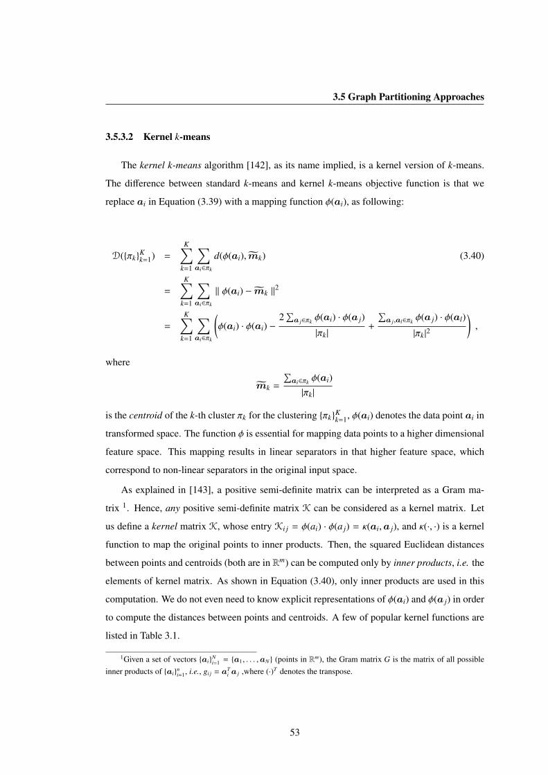
3.5 Graph Partitioning Approaches
3.5.3.2 Kernel k-means
The kernel k-means algorithm [142], as its name implied, is a kernel version of k-means.
The difference between standard k-means and kernel k-means objective function is that we
replace ai in Equation (3.39) with a mapping function φ(ai), as following:
D(πkKk=1) =
K∑k=1
∑ai∈πk
d(φ(ai), mk) (3.40)
=
K∑k=1
∑ai∈πk
‖ φ(ai) − mk ‖2
=
K∑k=1
∑ai∈πk
(φ(ai) · φ(ai) −
2∑
a j∈πk φ(ai) · φ(a j)
|πk|+
∑a j,al∈πk φ(a j) · φ(al)
|πk|2
),
where
mk =
∑ai∈πk φ(ai)|πk|
is the centroid of the k-th cluster πk for the clustering πkKk=1, φ(ai) denotes the data point ai in
transformed space. The function φ is essential for mapping data points to a higher dimensional
feature space. This mapping results in linear separators in that higher feature space, which
correspond to non-linear separators in the original input space.
As explained in [143], a positive semi-definite matrix can be interpreted as a Gram ma-
trix 1. Hence, any positive semi-definite matrix K can be considered as a kernel matrix. Let
us define a kernel matrix K, whose entry Ki j = φ(ai) · φ(a j) = κ(ai,a j), and κ(·, ·) is a kernel
function to map the original points to inner products. Then, the squared Euclidean distances
between points and centroids (both are in Rm) can be computed only by inner products, i.e. the
elements of kernel matrix. As shown in Equation (3.40), only inner products are used in this
computation. We do not even need to know explicit representations of φ(ai) and φ(a j) in order
to compute the distances between points and centroids. A few of popular kernel functions are
listed in Table 3.1.
1Given a set of vectors aiNi=1 = a1, . . . ,aN (points in Rm), the Gram matrix G is the matrix of all possible
inner products of aini=1, i.e., gi j = aT
i a j ,where (·)T denotes the transpose.
53

3. GRAPH-BASED IMAGE REPRESENTATION
Table 3.1: Examples of commonly used kernel functions.
Polynomial Kernel κ(ai,a j) = (ai · a j + c)d
Gaussian Kernel κ(ai,a j) = exp(− ‖ ai − a j ‖
2 /2α2)Sigmoid Kernel κ(ai,a j) = tanh
(c(ai · a j) + θ
)
3.5.3.3 Weighted kernel k-means
In the weighted graph, the edge weights play an important role. For that reason, a weighted
version of the kernel k-means is used for graph partitioning in our applications.
The weighted kernel k-means was first introduced in [123], its objective function can be
written as the minimization of:
D(πkKk=1) =
K∑k=1
∑ai∈πk
wi d(φ(ai), mk) =
K∑k=1
∑ai∈πk
wi ‖ φ(ai) − mk ‖2 , (3.41)
where
mk =
∑ai∈πk wiφ(ai)∑
ai∈πk wi= argminz
∑ai∈πk
wi ‖ φ(ai) − z ‖2
represents the “best” cluster representative, and the weights are non-negative (wi > 0). Sim-
ilarly in Equation (3.40), the clusters can be computed by using the entries of kernel matrix
since the term
wi ‖ φ(ai) − mk ‖2 = φ(ai) · φ(ai) −
2∑
a j∈πk w jφ(ai) · φ(a j)∑a j∈πk w j
+
∑a j,al∈πk w jwlφ(a j) · φ(al)
(∑
a j∈πk w j)2
= Kii −2∑
a j∈πk w jKi j∑a j∈πk w j
+
∑a j,al∈πk w jwlK jl
(∑
a j∈πk w j)2 , (3.42)
only requires computing inner products.
The basic graph partitioning procedure by weighted kernel k-means is illustrated in Algo-
rithm 2. If the number of data points is n, the data dimension is m, the total number of iterations
is τ, then the time complexity of the algorithm is O(n2(τ + m)). The complexity can be further
reduced to O(nz · τ), if kernel matrix K is a sparse matrix, with nz as the number of nonzero
entries in the matrix (nz = n2 for a dense kernel matrix).
54

3.5 Graph Partitioning Approaches
Algorithm 2 Graph clustering by weighted kernel k-means
Require: Weighted graph G = (V, E,W), kernel matrix K, fixed clusters number K, optionalinitial clusters π(0)
c kc=1, iteration counter t, optional maximum number of iterations tmax.
Ensure: Output final clusters πkKk=1 .
1: set t ← 0, initialize the K clusters π01, . . . , π
0K if not given.
2: while t < tmax or not converged do3: for each graph node ai ∈ V do4: for every cluster k do5: compute wi d(φ(ai), mk) in Equation (3.42)6: end for7: c∗(ai) = argmink
(wi d(φ(ai)
)8: end for9: Update the clusters as π(t+1)
c = a : c∗(ai) = c .10: set t ← t + 111: end while12: output final clusters π(t)
k Kk=1 .
3.5.3.4 Multilevel weighted kernel k-means algorithm
The multilevel scheme Dhillon et al. developed a general graph clustering algorithm based
on multilevel methods [11]. This algorithm works for a wide class of graph clustering ob-
jectives. It includes three phases: coarsening, based-clustering and refinement. We describe
each of these phases in more detail below. An illustration of this multilevel K-way partitioning
scheme for irregular graphs is shown in Figure 3.11.
Coarsening phase Let us denote the edge weight between vertices x and y by e(x, y), weights
of vertices x and y are w(x) and w(y) respectively. We define the weight of a vertex as its degree
(see Definition 9), in case of Normalized Cuts.
Starting with the initial graph G0 = (V0, E0,W0), the coarsening phase repeatedly trans-
forms the graph into smaller graphs G1,G2, . . . ,Gm such that |V0| > |V1| > . . . > |Vm|. During
coarsening phase, a set of nodes of the graph Gl is combined into a single super vetex in a
coarser graph Gl+1. The super vertex is formed in such a way: Given an unmarked vertex x in
graph Gl = (Vl, El,Wl), we seek to combine the vertex x with another vertex y ∈ Vl that assures
55

3. GRAPH-BASED IMAGE REPRESENTATION
Figure 3.11: An overview of the kernel-based multilevel algorithm for graph clustering proposedby Dhillon et al. [11], here K = 6. A part of this image is excerpted from [12].
the following criterion:
max(e(x, y)w(x)
+e(x, y)w(y)
). (3.43)
The weights of the super vertices of the coarser graph reflect the weights of the vertices of the
finer graph. This procedure is described as in Algorithm 3.
Base clustering phase After the coarsening phase, we get the coarsest graph Gm that contains
much smaller number of vertices than the initial graph G0. We can specify how smaller Gm to be
by using a pre-defined parameter. In the experiments, we keep coarsening the graph as long as
the number of graph nodes is sufficiently larger than max( |V |5K , 20), where K is a fixed number of
desired clusters. Once the coarsening phase is finished, we can apply different graph clustering
objectives (see Section 3.5.2.4) on the coarsest graph until K clusters are obtained. We call this
phase as “base clustering”. In the present work, we use the NCuts objective function, as defined
in Equation (3.34). This initial clustering is efficient in terms of speed, since the coarsest graph
Gm is significantly smaller that the input graph G0.
Refinement phase In the final refining phase, given a graph Gl, we build the finer graph Gl−1
(Gl−1 is the same graph used in level l − 1 in the coarsening phase). An initial clustering for
the graph Gl−1 is defined in the following way: If a super vertex is in the cluster k in Gl, then
56

3.5 Graph Partitioning Approaches
all nodes in Gl−1 that formed this super vertex are in cluster k. At all levels except the coarsest
level of Gm, the initial clustering of the graph is extended from the previous coarser level.
As justified in [141], both a general weighted kernel k-means objective and a weighted
graph partitioning objective can be mathematically expressed as matrix trace maximizations
problem. This equivalence has important significations: we can directly apply the weighted
kernel k-means algorithm, as described in Algorithm 2, to optimize the graph partitioning ob-
jectives such as Ratio cut, Normalized cut and ratio association etc, and vice versa. Hence,
after the initialization step, we run the weighted kernel k-means algorithm recursively to refine
the clustering from the coarsest graph Gm to the original graph G0. The algorithm can converge
very quickly at each level, due to good initial clustering.
Algorithm 3 Graph clustering in coarsening phaseRequire: Initial graph G0 = (V0, E0,W0).Ensure: Output a series of smaller graphs G1,G2, . . . ,Gm on coarse level l = 1, 2, . . . ,m.
1: set t ← 0, ∀x ∈ V0, unmark(x).2: while l < m do3: for current level l with its corresponding graph Gl = (Vl, El,Wl) do4: unmark(x), x ∈ Vl
5: repeat6: for each unmarked x ∈ Vl do7: if @y ∈ Vl that is unmarked then8: mark(x)9: else
10: find y that satisfies the Equation (3.43)11: super vertex z← merge x and y12: w(z) = w(x) + w(y)13: end if14: end for15: until marked(x) is true, ∀x ∈ Vl
16: end for17: end while
57

3. GRAPH-BASED IMAGE REPRESENTATION
3.5.3.5 Kernel k-means in applications
In real life data set, the structures are often hard to be separated in linear space. Kernel
k-means (KKM) has been suitable to identify clusters that are non-linearly separable in input
space. For instance, Dhillon et al. [123] applied KKM to diametrical clustering of gene expres-
sion and handwriting recognition, and achieved good results. One of disadvantages for KKM
is that the number of cluster centres need to be predefined.
3.6 Illustrations of Graph Partitioning
In this Section, several examples are enumerated on the graph partitioning results obtained
by using the aforementioned three different partitioning methods. The images are selected
from six categories: “accordion” (Figure 3.12 and Figure 3.18), “faces” (Figure 3.13 and Fig-
ure 3.19), “pagoda” (Figure 3.14 and Figure 3.20), “trilobite” (Figure 3.14 and Figure 3.20),
“cellphone” (Figure 3.16 and Figure 3.22), and “motorbikes” (Figure 3.17 and Figure 3.23) in
Caltech-101 dataset [144]. Here we only list five examples per category. More details will be
discussed in Section 6.9.1 of the Chapter 6.
Figure 3.12, Figure 3.13, Figure 3.14, Figure 3.15, Figure 3.16 and Figure 3.17 present
images that are divided into 4 subgraphs with three different methods: either Graph Cuts (GC)
or Normalized Cuts (NC) or kernel k-means (KKM). The name of each image is marked on the
left side of the figure.
In like manner, Figure 3.18, Figure 3.19, Figure 3.20, Figure 3.21, Figure 3.22 and Fig-
ure 3.23 illustrate the partitioning results in which each image is composed of 16 irregular
subgraphs. The 1-3 columns in each figure correspond to the partitioning results obtained via
Graph Cuts (GC), Normalized Cut (NC), kernel k-means (KKM) respectively.
Some observations on these (eight) figures: 1) There exist very small subgraphs that contain
only a few of isolated points in partitions, e.g. an isolated green point on image accordion0031
(GC) in the Figure 3.12; two scattered red points in pagoda0035 (GC) and pagoda0047 (GC)
in Figure 3.14; two isolated points in blue and garnet red color respectively in faces0039 (GC)
in Figure 3.19 etc. 2) In case of 4 partitions per image, object of interest can be represented
by only one or two subgraphs. 3) Despite the weights (objective function) defined on the
graph edges are the same, the partitioning results (obtained subgraphs) vary from individual to
individual in the same image.
58

3.6 Illustrations of Graph Partitioning
acco
rdio
n003
1ac
cord
ion0
032
acco
rdio
n004
1ac
cord
ion0
053
acco
rdio
n005
5
Graph Cuts Normalized Cut KKM
Figure 3.12: Examples of graph partitioning in 4 irregular subgraphs on five examples in category“accordion” from Caltech-101 dataset by three methods: Graph Cuts (GC), Normalized Cut (NC),kernel k-means (KKM). This figure is better viewed in color.
59

3. GRAPH-BASED IMAGE REPRESENTATION
face
s003
2f a
ces0
036
f ace
s003
8f a
ces0
039
f ace
s004
9
Graph Cuts Normalized Cut KKM
Figure 3.13: Examples of graph partitioning in 4 irregular subgraphs on five examples in category“faces” from Caltech-101 dataset by three methods: Graph Cuts (GC), Normalized Cut (NC),kernel k-means (KKM). This figure is better viewed in color.
3.7 Conclusions
In this Chapter, we have presented three typical graph partitioning approaches: Graph Cuts,
Normalized Cuts, and kernel based multilevel graph clustering algorithm. These three methods
will be used in our proposed model in the next Chapter 4 and be compared in Chapter 6.
60
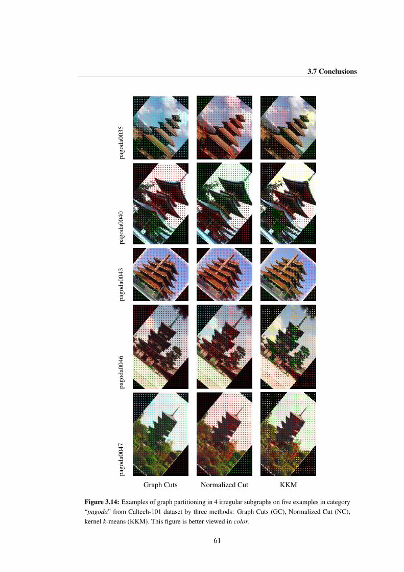
3.7 Conclusions
pago
da00
35pa
goda
0040
pago
da00
43pa
goda
0046
pago
da00
47
Graph Cuts Normalized Cut KKM
Figure 3.14: Examples of graph partitioning in 4 irregular subgraphs on five examples in category“pagoda” from Caltech-101 dataset by three methods: Graph Cuts (GC), Normalized Cut (NC),kernel k-means (KKM). This figure is better viewed in color.
61

3. GRAPH-BASED IMAGE REPRESENTATION
trilo
bite
0037
trilo
bite
0041
trilo
bite
0056
trilo
bite
0064
trilo
bite
0072
Graph Cuts Normalized Cut KKM
Figure 3.15: Examples of graph partitioning in 4 irregular subgraphs on five examples in category“trilobite” from Caltech-101 dataset by three methods: Graph Cuts (GC), Normalized Cut (NC),kernel k-means (KKM). This figure is better viewed in color.
62

3.7 Conclusions
cellp
hone
0032
cellp
hone
0035
cellp
hone
0049
cellp
hone
0051
cellp
hone
0059
Graph Cuts Normalized Cut KKM
Figure 3.16: Examples of graph partitioning in 4 irregular subgraphs on five examples in category“cellphone” from Caltech-101 dataset by three methods: Graph Cuts (GC), Normalized Cut (NC),kernel k-means (KKM). This figure is better viewed in color.
63

3. GRAPH-BASED IMAGE REPRESENTATION
mot
orbi
kes0
042
mot
orbi
kes0
043
mot
orbi
kes0
047
mot
orbi
kes0
055
mot
orbi
k es0
059
Graph Cuts Normalized Cut KKM
Figure 3.17: Examples of graph partitioning in 4 irregular subgraphs on five examples in category“motorbikes” from Caltech-101 dataset by three methods: Graph Cuts (GC), Normalized Cut (NC),kernel k-means (KKM). This figure is better viewed in color.
64

3.7 Conclusions
acco
rdio
n003
1ac
cord
ion0
032
acco
rdio
n004
1ac
cord
ion0
053
acco
rdio
n005
5
Graph Cuts Normalized Cut KKM
Figure 3.18: Examples of graph partitioning in 16 irregular subgraphs on five examples in category“accordion” from Caltech-101 dataset by three methods: Graph Cuts (GC), Normalized Cut (NC),kernel k-means (KKM). This figure is better viewed in color.
65

3. GRAPH-BASED IMAGE REPRESENTATION
face
s003
2fa
ces0
036
face
s003
8f a
ces0
039
f ace
s004
9
Graph Cuts Normalized Cut KKM
Figure 3.19: Examples of graph partitioning in 16 irregular subgraphs on five examples in category“faces” from Caltech-101 dataset by three methods: Graph Cuts (GC), Normalized Cut (NC),kernel k-means (KKM). This figure is better viewed in color.
66

3.7 Conclusions
pago
da00
35pa
goda
0040
pago
da00
43pa
goda
0046
pago
da00
47
Graph Cuts Normalized Cut KKM
Figure 3.20: Examples of graph partitioning in 16 irregular subgraphs on five examples in category“pagoda” from Caltech-101 dataset by three methods: Graph Cuts (GC), Normalized Cut (NC),kernel k-means (KKM). This figure is better viewed in color.
67

3. GRAPH-BASED IMAGE REPRESENTATION
trilo
bite
0037
trilo
bite
0041
trilo
bite
0056
trilo
bite
0064
trilo
bite
0072
Graph Cuts Normalized Cut KKM
Figure 3.21: Examples of graph partitioning in 16 irregular subgraphs on five examples in category“trilobite” from Caltech-101 dataset by three methods: Graph Cuts (GC), Normalized Cut (NC),kernel k-means (KKM). This figure is better viewed in color.
68

3.7 Conclusions
cellp
hone
0032
cellp
hone
0035
cellp
hone
0049
cellp
hone
0051
cellp
hone
0059
Graph Cuts Normalized Cut KKM
Figure 3.22: Examples of graph partitioning in 16 irregular subgraphs on five examples in category“cellphone” from Caltech-101 dataset by three methods: Graph Cuts (GC), Normalized Cut (NC),kernel k-means (KKM). This figure is better viewed in color.
69

3. GRAPH-BASED IMAGE REPRESENTATION
mot
orbi
kes0
042
mot
orbi
kes0
043
mot
orbi
k es0
047
mot
orbi
kes0
055
mot
orbi
k es0
059
Graph Cuts Normalized Cut KKM
Figure 3.23: Examples of graph partitioning in 16 irregular subgraphs on five examples in category“motorbikes” from Caltech-101 dataset by three methods: Graph Cuts (GC), Normalized Cut (NC),kernel k-means (KKM). This figure is better viewed in color.
70

Chapter 4
Bag-of-Bags of Words Model
In this chapter, we introduce the proposed ‘Bag-of-Bags of Words’ model. We aim to model
an image by graphs. An image is first represented as an undirected weighted graph. This initial
image graph is partitioned into a fixed number of subgraphs that describe similar components
in the image. Each subgraph is further described by bag-of-words features. Finally, a novel
graph-based image representation model derives from those subgraphs descriptors.
4.1 Overview of the Bag-of-Bags of Words Model
Before introducing our model formally, here we explain its general principle and construc-
tion. Bag-of-Bags of Words for a given image, is a set of Bag-of-Words (BoWs). Each of
BoWs is computed on vertices of image subgraph obtained by irregular partition of image
graph. Next, the rationale for our “Bag-of-Bags” is in the correlation with two notable con-
cepts: 1) Bag of Features (BoF) [31], i.e., the unordered set of local descriptors extracted from
an image. These local features are extracted from either fixed grid points or detected points of
interest in the image. 2) “Bag-of-Words” (BoW) model, as proposed by Sivic et al. [16] and
Csurka et al. [80]. Indeed, our description is a set of unordered features (BoF), each feature
being a BoW built upon an image subgraph.
We will now describe a methodology for the construction of BBoW model. Then in Sec-
tion 4.1.4, we will formalize the model more thoroughly. In Section 4.3, we present our contri-
bution regarding the use of our BBoW model for image retrieval.
The BBoW model of an image is built as follows: 1) Select a reduced number of pixels V;
2) Build an initial image graph G; 3) Partition the graph G into K subgraphs; 4) Compute a
71

4. BAG-OF-BAGS OF WORDS MODEL
signature for each subgraph.
The signature of a subgraph is a histogram of codeword occurrences, obtained by assigning
the feature vector of each graph node in this subgraph to the closest visual word in the code-
book. Hence, an image composed of K subgraphs is characterized by a set of K histograms. An
overview of the proposed framework is shown in Figure 4.1. In the following, we will detail
how to construct the BBoW model step by step.
Figure 4.1: The diagram of construction of Bag-of-Bags of Words model.
4.1.1 Feature Extraction
Firstly, given an input image I j, we extract local image features from image patch. Different
types of popular descriptors such as SIFT [2] or SURF [35] etc., can be used to describe local
features as vectors from the patches. The local features are extracted from either prominent
keypoints or dense sampling points on regular grid.
In case of prominent keypoints approach, any interest points detection algorithms can be
used to extract keypoints. In the present work, we use SURF [35] as image descriptors to
extract feature points under the mask of the image for the interest object. In order to avoid
these points are too close to each other in positions, we filter those points by keeping only the
most prominent keypoint over any 10-pixels diametrical region. The obtained filtered keypoints
P = p1, ..., pn are selected as vertices of the initial image graph.
72

4.1 Overview of the Bag-of-Bags of Words Model
In case of dense sampling strategy, the image features are computed using only the SIFT [2]
feature vectors of all dense sampling points. We use an overlap between patches of 50% to
reach a compromise between repeatability of interest points and reasonable size of features. Its
corresponding pipeline is illustrated in Figure 4.2.
Figure 4.2: The dense points sampling approach in BBoW model.
4.1.2 Graph Construction
Secondly, we build an undirected weighted graph G j = (V j, E j,W j) on the image I j. We
call it the initial image graph.
As defined in Section 3.3.1 and Section 4.1.1, the graph nodes are positioned on either
filtered prominent keypoints or on the dense sampling points at a regular grid. Once these graph
nodes are localized, we head to generate edges and define the corresponding weights of these
edges. The graph edges represent relationship between graph nodes. They are generated by
linking these vertices in specified neighbourhood system (see Figure 3.3), as we have discussed
in Section 3.3.2. In such a way, one connected image graph is generated for each image.
The edge weight reflects the similarity between the two nodes of that edge. Such a similarity
measurement depends on a specified objective function. Let us denote by W, a symmetric
matrix of edge weights between all nodes. Then the edge weights are represented by non-zero
entries of this affinity matrix W, see Equation (3.1).
73

4. BAG-OF-BAGS OF WORDS MODEL
4.1.3 Irregular Subgraphs
Thirdly, the initial image graph is separated into a fixed number of K partitions (sub-
graphs) [12] via graph partitioning.
Case study: prominent keypoints approach in BBoW model Let us denote G = (V, E)
a graph generated by the Delaunay triangulation. The vertices set V contains all the feature
points, i.e. V = P. The edges set E contains all unordered pairs of points p, q that are
neighbours in the Delaunay graph. We want to separate graph G into K smaller graphs via
Graph Cuts. This can be formulated as a labeling problem: given a points set P in image I j,
and a label set L = l1, . . . , lK, for each p ∈ P, we are looking for its label l(p) = lp ∈ L.
In order to be consistent with the image content, we construct a set of sub-graphs g j,1, · · · , g j,K,
according to the following requirements: each sub-graph, 1) should be as compact as possible;
2) should have, as much as possible, a uniform color. To solve this labeling problem, we
minimize the energy function defined in Equation (3.11) of Chapter 3, via α-expansion [8]
algorithm in Graph Cuts. An illustration will be given in Section 6.4 of the Chapter 6.
Case study: dense sampling approach in BBoW model Since prominent keypoints ap-
proach in BBoW model does not exhibit promising result, we hence go for dense sampling
approach in the following discussion. An example of irregular subgraphs obtained by dense
sampling approach in BBoW model, is illustrated in Figure 4.3.
As discussed in Section 3.4, we assess three standard approaches for irregular graph parti-
tions in the BBoW model. These methods are: Graph Cuts, Normalized Cuts and kernel-based
multilevel weighted graph cuts. Here we stress that the idea of applying graph partitioning
methods to image graph is not novel, e.g., [124, 145, 146]. Our contribution lies in rigorously
demonstrating that irregular (sub)graph-based representation is well-suited to pre-clustering
interest points accounting for color and texture similarity, and that this representation extends
BoWs model with spatial layouts, combines the advantages of SPM as well.
4.1.4 Bag-of-Bags of Words Description
Fourthly, we compute image signatures by designing a measure for describing these sub-
graphs. As in the standard BoW approach, we first build a codebook from all image features
in a training image dataset. The codebook is computed by using k-means clustering method
74

4.2 (Dis-)Similarity Measurement between Histograms
Figure 4.3: The obtained irregular subgraphs via graph partitioning.
over these features vectors, therefore, it is independent from any partitioning scheme. The
codewords C then correspond to the centres of the learned clusters. A bag of visual word
representation, i.e. a histogram of word frequencies, is then assigned to each subgraph.
Let us denote by H j,k a signature of the subgraph g j,k (k = 1, . . . ,K) in image I j. H j,k
is a Bag-of-Words histogram, obtained by assigning the SIFT (or SURF) features within the
subgraph g j,k to the nearest codeword (hard assignment), as in the standard BoW approach.
Hence, the BBoW representation of image I j for this partitioning is a histogram vector H j =
H j,1, . . . ,H j,K of length K, normalized by the number of nodes in the initial image graph G j.
With such a normalization, the larger subgraphs are privileged. We call H j the “Bag-of-Bags
of Words” (BBoW) description. See Figure 4.4.
4.2 (Dis-)Similarity Measurement between Histograms
A histogram is a collection of bins that count a frequency distribution of data. This im-
portant statistical characteristic is useful to represent the distribution of pixel intensity, color
and texture of images. The histogram representation has several advantages. It is easy to com-
pute, intuitive and invariant to translation and rotation about view plane etc. When images
are characterized by histograms, comparing images is equivalent to computing the distances or
(dis-)similarities between their model histograms.
75
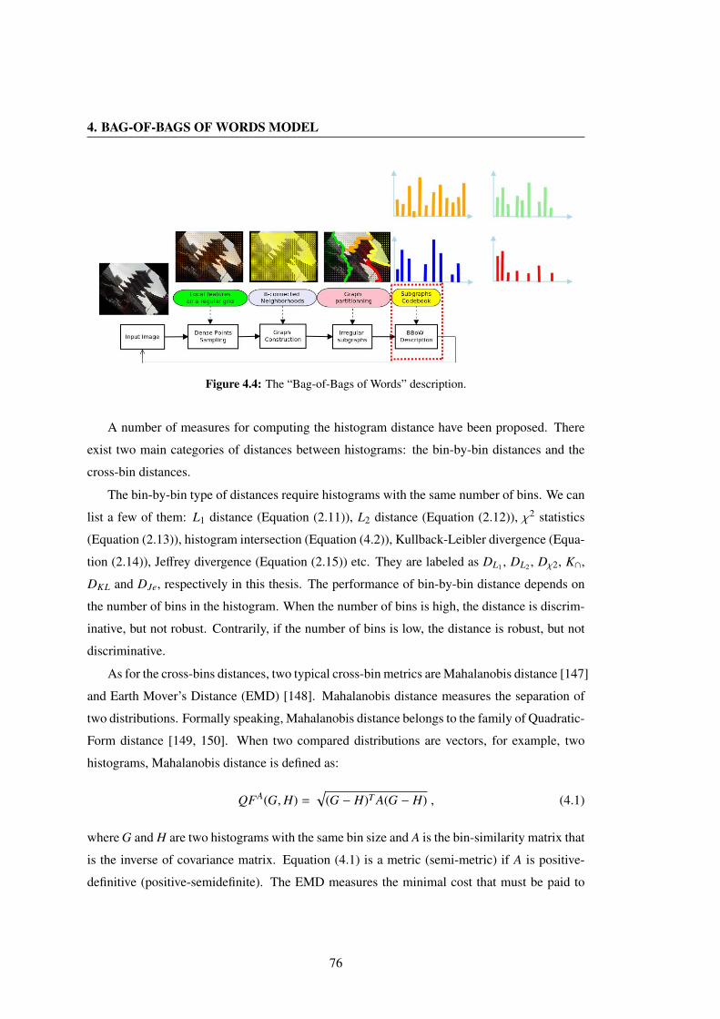
4. BAG-OF-BAGS OF WORDS MODEL
Figure 4.4: The “Bag-of-Bags of Words” description.
A number of measures for computing the histogram distance have been proposed. There
exist two main categories of distances between histograms: the bin-by-bin distances and the
cross-bin distances.
The bin-by-bin type of distances require histograms with the same number of bins. We can
list a few of them: L1 distance (Equation (2.11)), L2 distance (Equation (2.12)), χ2 statistics
(Equation (2.13)), histogram intersection (Equation (4.2)), Kullback-Leibler divergence (Equa-
tion (2.14)), Jeffrey divergence (Equation (2.15)) etc. They are labeled as DL1 , DL2 , Dχ2, K∩,
DKL and DJe, respectively in this thesis. The performance of bin-by-bin distance depends on
the number of bins in the histogram. When the number of bins is high, the distance is discrim-
inative, but not robust. Contrarily, if the number of bins is low, the distance is robust, but not
discriminative.
As for the cross-bins distances, two typical cross-bin metrics are Mahalanobis distance [147]
and Earth Mover’s Distance (EMD) [148]. Mahalanobis distance measures the separation of
two distributions. Formally speaking, Mahalanobis distance belongs to the family of Quadratic-
Form distance [149, 150]. When two compared distributions are vectors, for example, two
histograms, Mahalanobis distance is defined as:
QFA(G,H) =√
(G − H)T A(G − H) , (4.1)
where G and H are two histograms with the same bin size and A is the bin-similarity matrix that
is the inverse of covariance matrix. Equation (4.1) is a metric (semi-metric) if A is positive-
definitive (positive-semidefinite). The EMD measures the minimal cost that must be paid to
76
4.3 BBoW on Single Level for Image Retrieval
transform one distribution into the other. This distance can operate on variable-length repre-
sentations of the distribution. It is widely used in content-based image retrieval to compute
distances between the color histograms of two images [151].
For couples of the aforementioned distances, they have been formulated in Section 2.1.7
of the Chapter 2. In the following, we will give emphasis to an important similarity measure -
histogram intersection, which is adopted in the present work.
Histogram intersection: Let us denote by G = g1, . . . , gB and H = h1, . . . , hB, are two
normalized histograms with B bins. Particularly, these two histograms are normalized to one,
i.e.B∑
b=1
gb =
B∑b=1
hb = 1. Histogram intersection (HI) is defined as:
K∩(G,H) =
B∑b=1
min(gb, hb) . (4.2)
Histogram intersection was first introduced by Swain et al. [44] as a technique of comparing
image and model histograms for color indexing. It is a useful similarity measure for images and
is even proved to be an effective kernel for machine learning [152]. The similarity measures in
the BBoW model are based on histogram intersection.
There is an alternative way to compute HI:
K∩(G,H) =12
B∑b=1
(gb + hb − |gb − hb|) , (4.3)
which improves computation efficiency, e.g. programming for a GPU, since we do not need
to explicitly compare the values of each bin. We verify the equivalence of Equation (4.2) and
Equation (4.3) in the Appendix D.
4.3 BBoW on Single Level for Image Retrieval
We now review how to apply the bag-of-bags of words model for image retrieval on a single
level of a partition.
In the framework of content-based image retrieval (CBIR), the most common method for
comparing two images is using either a similarity metric or an image distance measure. Both
of them can be in various dimensions. And they can consider the similarity of color, texture,
shape etc. or in a combination of them in images. The distance measure is negatively correlated
77
4. BAG-OF-BAGS OF WORDS MODEL
with the corresponding similarity metric. That is to say, the more two images are similar, the
lower the distance value will be. For example, the distance is zero if two images are exactly
matched, i.e., they are identical.
In the BBoW model, after image graph partitioning, each image contains a fixed number
of K subgraphs. The image is thus represented by K BoVW histograms (subgraph signatures).
Using histograms to describe subgraphs, a comparison between two images Ii and I j becomes
equivalent to similarity search when comparing histogram signatures of their subgraphs. We
have adopted two strategies to define the similarity between images. We will explain the two
strategies in the following Section.
4.3.1 Co-occurrence Criteria
The first strategy to compare the two sets of subgraphs from two images consists in using
co-occurrence criteria such as those defined in [111].
We adopt the idea of RootSIFT [33] by first L1 normalizing the histograms and then
computing the histogram intersection of them. Since any image Ii is represented by a set
of histograms of its subgraphs Hi = Hi,1, · · · ,Hi,K; a (dis)similarity measure between two
(sub)graphs can be easily computed as we just need to compare their histogram signatures.
In such a way, we relate the similarity between two images with the similarity between BoW
histograms of the subgraphs in two images.
We have experimented different strategies to combine the K × K distances between a pair
of query image Ii, and database image I j from their corresponding histogram sets Hi and H j:
minimum, resp. sum of min, resp. mean, resp. median, resp. sum, resp. maximum, etc. of all
distances.
To compare two images Ii and I j that are composed of K subgraphs for each, we define a
series of similarity measures. We detail them as follows:
S min(Ii, I j) = mink=1,...,K
mink′=1,...,K
B∑b=1
min(Hi,k(b),H j,k′(b)) , (4.4)
S sum-of-mins(Ii, I j) =
K∑k=1
mink′=1,...,K
B∑b=1
min(Hi,k(b),H j,k′(b)) , (4.5)
S sum-of-means(Ii, I j) =
K∑k=1
meank′=1,...,K
B∑b=1
min(Hi,k(b),H j,k′(b)) , (4.6)
78

4.3 BBoW on Single Level for Image Retrieval
S sum-of-medians(Ii, I j) =
K∑k=1
mediank′=1,...,K
B∑b=1
min(Hi,k(b),H j,k′(b)) , (4.7)
S sum(Ii, I j) =
K∑k=1
K∑k′=1
B∑b=1
min(Hi,k(b),H j,k′(b)) , (4.8)
S sum-of-maxima(Ii, I j) =
K∑k=1
maxk′=1,...,K
B∑b=1
min(Hi,k(b),H j,k′(b)) . (4.9)
Our experiments have shown a better behaviour with Equation (4.4). We will discuss the
experimental results later in Section 6.4 of Chapter 6. This promising results based on Equa-
tion (4.4) promoted our second strategy in the Section 4.3.2.
In summary, image comparison via the co-occurrence criteria can be described in Algo-
rithm 4.
Algorithm 4 Image comparison via the co-occurrence criteria
Require: Given Image Ii with its K subgraphs gi,kKk=1 and I j with its K subgraphs g j,k′
Kk′=1
Ensure: Return a similarity score between image Ii and I j
1: for each subgraph gi,k in image Ii do2: compute the BoVW histogram hi,k of the corresponding subgraph3: end for4: for each subgraph g j,k′ in image I j do5: compute the BoVW histogram h j,k′ of the corresponding subgraph6: end for7: Similarity(Ii, I j) = S (∗)(Ii, I j), where (∗) is one of the co-occurrence criteria defined in
Section 4.3.1.
4.3.2 Weighted Bipartite Graph Matching
As discuss in previous Section, we compare images through comparing histogram signa-
tures of their subgraphs. Indeed, the subgraph attributed to label k can be at any position in
the image, see Figure 4.5. The spatial arrangement is lost if an image in a database undergoes
rotation, for instance. Hence, in order to overcome this issue, we cannot match histograms of
the subgraphs directly after the graph partitioning steps in BBoW model. We therefore need to
find optimal subgraphs matching between pairs of images so as to reorganize the histograms in
the BBoW description.
79
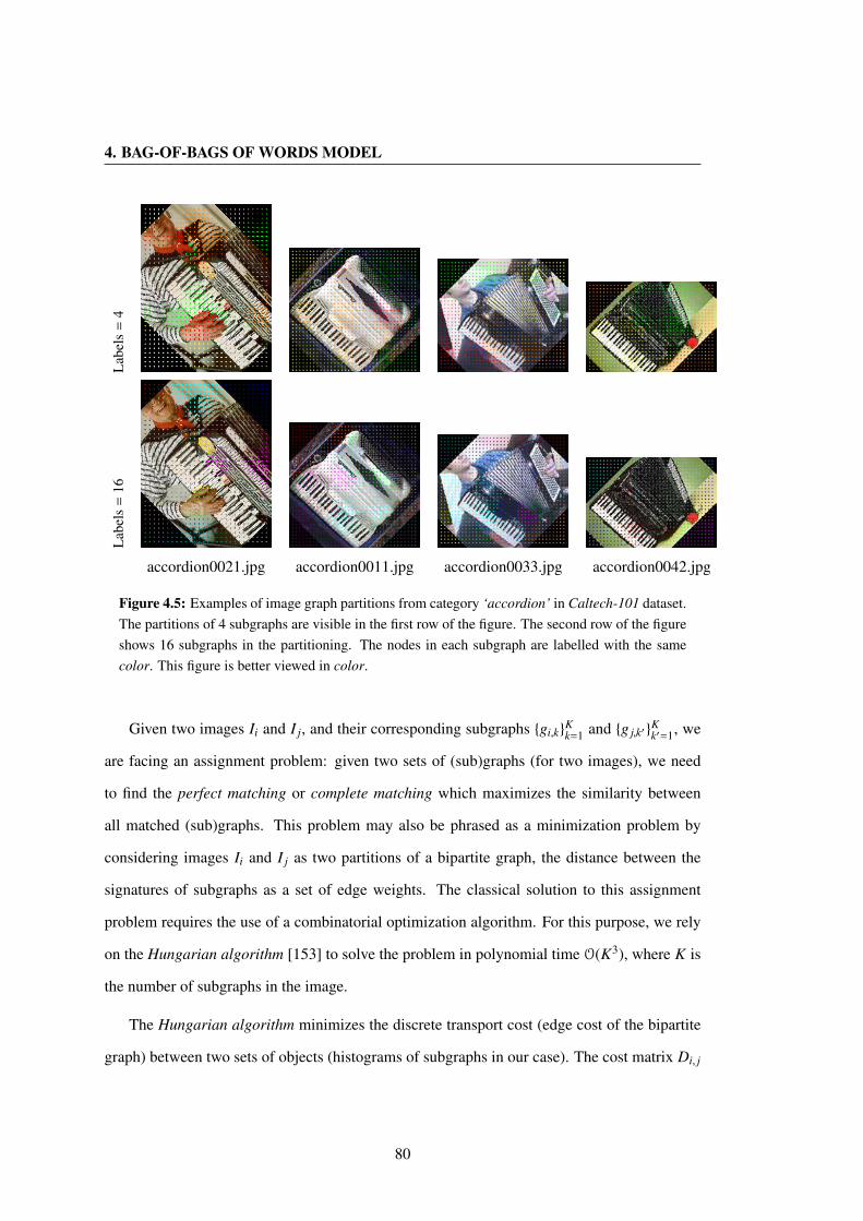
4. BAG-OF-BAGS OF WORDS MODEL
Lab
els
=4
Lab
els
=16
accordion0021.jpg accordion0011.jpg accordion0033.jpg accordion0042.jpg
Figure 4.5: Examples of image graph partitions from category ‘accordion’ in Caltech-101 dataset.The partitions of 4 subgraphs are visible in the first row of the figure. The second row of the figureshows 16 subgraphs in the partitioning. The nodes in each subgraph are labelled with the samecolor. This figure is better viewed in color.
Given two images Ii and I j, and their corresponding subgraphs gi,kKk=1 and g j,k′
Kk′=1, we
are facing an assignment problem: given two sets of (sub)graphs (for two images), we need
to find the perfect matching or complete matching which maximizes the similarity between
all matched (sub)graphs. This problem may also be phrased as a minimization problem by
considering images Ii and I j as two partitions of a bipartite graph, the distance between the
signatures of subgraphs as a set of edge weights. The classical solution to this assignment
problem requires the use of a combinatorial optimization algorithm. For this purpose, we rely
on the Hungarian algorithm [153] to solve the problem in polynomial time O(K3), where K is
the number of subgraphs in the image.
The Hungarian algorithm minimizes the discrete transport cost (edge cost of the bipartite
graph) between two sets of objects (histograms of subgraphs in our case). The cost matrix Di, j
80
4.3 BBoW on Single Level for Image Retrieval
between the pair of images Ii and I j reads:
Di, j =
d11
i, j . . . d1Kri, j
...
dKr1i, j . . . dKrKr
i, j
, (4.10)
where
dk,li, j =
B∑b=1
|Hi,k(b) − H j,l(b)|
is the L1 distance between Hi,k and H j,l, which corresponds to the use of histogram intersection.
The proof can be found in the Claim B of the Appendix D.
Figure 4.6 shows a toy example illustrating the subgraph matching process. Given two im-
age Ii and I j and their BBoW description Hi = Hi,a,Hi,b,Hi,c,Hi,d, H j = H j,1,H j,2,H j,3,H j,4,
the histogram distance of any pair of subgraphs between two images are computed. An exam-
ple of these distance values are shown as entries of a matrix in Figure 4.7. In this example,
the histogram distance between the subgraph gi,a of image Ii and the subgraph g j,1 of image
I j is 11. The Hungarian algorithm finds the minimum cost assignment for the cost matrix.
The subgraph gi,a in image Ii is optimal matched with the subgraph g j,1 in image I j, since the
transport cost (11) is the minimum value (underlined in red color) among these values of the
first row.
For computational efficiency, this matching step can be pre-computed once and stored.
A distance table and a label table can be constructed optionally, which records the distance
between all subgraphs being compared, and their corresponding labels. The distance values
are the entries in the aforementioned cost matrix Di, j. With this distance table, the procedure
of bipartite graph matching can be simplified to search in the look up tables. The storage
space being taken by the lookup tables is offset by the saved time, especially as the size of the
subgraphs increases.
After the processing step via the Hungarian algorithm, each label k of subgraph gi,k in im-
age Ii is associated to one label k′ = fi(k) of subgraph g j,k′ in image I j. We thus reorganize the
labels between the two sets of histograms Hi,kk=1, ..., K and H j,k′k′=1, ..., K in BBoW. There-
fore, the pairs of histograms to compare are identified. We call this step bipartite subgraphs
matching.
81

4. BAG-OF-BAGS OF WORDS MODEL
Figure 4.6: Find optimal subgraph matchingvia Hungarian algorithm.
Figure 4.7: An optimal assignmentfor a given cost matrix.
Finally, the similarity score of two images Ii and I j can be expressed by histogram inter-
section kernel, formally introduced in Equation (4.2):
K∩(Hi,k,H j,k
)=
B∑b=1
min(Hi,k(b),H j,k(b)
). (4.11)
Here k corresponds the k-th subgraph, B is the number of bins.
Essentially, for the first strategy of using co-occurrence criteria, e.g. Equation (4.4) etc., it
can be seen as the application of the Histogram Intersection kernel [44, 152] (Equation (4.11))
directly to the histograms of any orderless subgraphs between two compared images.
To sum up, the second strategy can be interpreted in Algorithm 5.
4.4 Summary of the BBoW model for CBIR
Figure 4.8 demonstrates the procedure of image comparison in Bag-of-Bags of Words
model from an image database. Note that both Algorithm 4 and Algorithm 5 require com-
puting the bag-of-visual-words histogram for each subgraph.
Figure 4.8: The process of CBIR from database in BBoW model.
82

4.5 Discussion and Conclusion
Algorithm 5 Image comparison via Hungarian algorithm to reorganize histograms
Require: Given Image Ii with its K subgraphs gi,kKk=1 and I j with its K subgraphs g j,k
Kk=1
Ensure: Return a similarity score between image Ii and I j
1: for each subgraph gi,k in image Ii do2: compute the BoVW histogram hi,k of the corresponding subgraph3: end for4: for each subgraph g j,k in image I j do5: compute the BoVW histogram h j,k of the corresponding subgraph6: end for7: Build Di, j in Equation (4.10)8: Run the Hungarian algorithm to reorganize histograms of subgraphs i.e., each label k of
subgraph gi,k in image Ii is associated to one label k′ = fi(k) of subgraph g j,k′ in image I j
9: Set Hi ← Hi,kk=1,...,K
10: Set H j ← Hi,k′k′=1,...,K
11: Similarity(Ii, I j) = K∩(Hi,H j)
4.5 Discussion and Conclusion
In the present Chapter, we have presented a novel model for image representation. The pro-
posed BBoW model with the aid of graphs, extends the classical bag-of-words (BoW ) model,
by embedding color homogeneity and limited spatial information through irregular partitions
of an image. The model well addresses fundamental limitations of the classical Bag-of-Words
model [16] and the regular structure of spatial pyramid representation [4]. We have also pro-
posed to embed spatial layout into our BBoW representation by bipartite subgraphs matching
via Hungarian algorithm. To the best of our knowledge, we are the first to apply Hungarian
algorithm to subgraphs matching on the task of spatial layout analysis in image representation.
We have observed that the generated subgraphs are often too small after graph partitioning
process. In such cases, subgraphs contain only a few of nodes. This makes the BBoW descrip-
tion less representative. In order to be more effective, we may consider removing these small
or inconsistent subgraphs. However, this technique will produce another problem: how to deal
with a set of histograms of different size in the final BBoW description. Again, if we choose a
different number of resolutions for different type of images, it also involves the same problem:
compare set of histograms of different size.
In the next Chapter, we propose to extend our model to multiple levels inspired by previous
83

4. BAG-OF-BAGS OF WORDS MODEL
works, such as Montanvert et al. [154].
84

Chapter 5
Irregular Pyramid Matching
In Chapter 4, we have introduced the proposed bag-of-bags of words (BBoW) model. The
BBoW model, is an approach based on irregular partitions over the image. An image is first
represented as a connected graph of local features on a regular grid of pixels. Next, irregular
partitions (subgraphs) of the image are further built by using graph partitioning methods. Each
subgraph in the partition is then represented by its own signature. The BBoW model with
the aid of graphs, extends the classical bag-of-words (BoW) model in image space instead
of feature space, by embedding color homogeneity and limited spatial information through
irregular partitions of an image. In this chapter, we extend this proposed model to pyramid
levels, leading to an approach that we call irregular pyramid matching.
5.1 BBoW on Pyramid Level
In this Section, we first introduce the graph partitioning scheme on multi-levels in the bag-
of-bags of words model. Then we describe the procedure of irregular pyramid matching.
5.1.1 Graph Partitioning Scheme
As in Spatial Pyramid Matching [4], we aim to build a pyramid of partitions at several
“resolutions” (r = 0 . . .R). At resolution r of image partitions, the image graph G j is split into
a set of Kr = 22r subgraphs grj,1, . . . , gr
j,K. We name it pyramidal image graph partitioning
scheme. An example is shown in Figure 5.1, where the initial image graph is divided into a
fixed number of subgraphs at different resolutions.
85

5. IRREGULAR PYRAMID MATCHING
Figure 5.1: A schematic illustration of the BBoW representation at each level of the pyramid. Atlevel 0, the decomposition has a single graph, and the representation is equivalent to the classicalBoW. At level 1, the image is subdivided into four subgraphs, leading to four features histograms,and so on. Each subgraph is represented by its own color in this figure. This figure is better viewedin color.
5.1.2 Irregular Pyramid Matching
In Section 4.1.4, the BBoW description is based on a fixed number of partitions at a single
level on the whole image. After the pyramidal image graph partitioning step, BoW histograms
are computed within each subgraph, then the histograms from all subgraphs are concatenated
together to generate the final representation of the image. Such an extension of BBoW model
to pyramid gives rise to a method we name irregular pyramid matching (IPM). In case where
only the level l = 0 is used to compute image signature, BBoW reduces to BoW representation.
5.2 BBoW on Pyramid Levels for Image Retrieval
After generating visual signature of the image on pyramid levels in BBoW model, we need
to define the corresponding similarity measures to compare images.
86

5.2 BBoW on Pyramid Levels for Image Retrieval
5.2.1 Similarity Measure
Once bipartite subgraphs matching is fulfilled, we can directly apply the level weighted
intersection as described in [4] to compare images:
κ(Ii, I j) = I(HR
i,k,HRj,k′
)+
R−1∑r=0
12R−r
(Ir − Ir+1)
=12R I
(H0
i,1,H0j,1)
+
R∑r=1
12R−r+1 I
(Hr
i,k,Hrj,k′
), (5.1)
where
I(Hr
i,k,Hrj,k′
)=
B∑b=1
min(Hr
i,k(b),Hrj,k′(b)
)is the histogram intersection function in [152], B is the bag of words codebook size, which is
related to the L1 norm [44]. k and k′ here are the indices of the corresponding subgraphs being
matched after rearrangement of histograms via Hungarian algorithm. The weight 12R−r allows
for penalizing low resolutions of a partition, reflecting the fact that higher levels localize the
features inside smaller graphs more precisely. Hence, in our approach, we propose to apply
directly the level weighted intersection to irregular partitions obtained by graph cuts methods,
following the idea of SPM [4].
5.2.2 Global Algorithm for Image Retrieval with BBoW model
After discussion, we summarize the global algorithm in BBoW model for its application
for image retrieval.
1. Local features extraction at interest point locations, or nodes in a dense grid.
(a) Prominent keypoints
(b) Dense points sampling
2. Codebook generation (dictionary is level independent, built off line).
3. Graph Construction (define graph nodes, weighted edges) for each image.
4. Partition the initial image graph into a fixed number of irregular subgraphs on multiple
resolution for each image.
5. Build BoW histograms of the subgraphs.
6. Compare images based on specific similarities measure.
87

5. IRREGULAR PYRAMID MATCHING
5.3 Discussion and Conclusion
In this Chapter, we have embedded our BBoW model into a pyramid approach. Hence, the
final signature of the image has been built as a concatenation of BoW histograms from each
level of the pyramid, where each BoW histogram is normalized by the number of nodes in the
initial image graph. With such a normalization, the larger subgraphs are privileged. We call it
Bag-of-Bags of Words (BBoW) description in pyramid. With such descriptors, we match graph
pyramid level by level. Hence, we always match the partitions of the same granularity. The
number of pyramid level is chosen to be the same in the database. Therefore, we do not have
any problem in matching images with different number of subgraph histograms.
Note that the Spatial Pyramid Matching [4] scheme partitions an image recursively into a
coarse-to-fine (sub)regions, i.e., their partitions are nested, as introduced in Section 2.3.2.1 of
Chapter 2. In contrast, our partitions are independent at each level in the BBoW model, see
Figure 5.2. Moreover, we keep the same resolution of images during partitioning. That means
we do not use a Gaussian pyramid [155–157] as main concept of pyramid does. The main
reason that we have adopted this strategy is attributed to avoid obtaining isolated (too small)
subgraphs, leading to the BBoW description less representative.
In the next Chapter, we will evaluate our model in different respects, especially, its appli-
cation for image retrieval.
88

5.3 Discussion and Conclusion
Figure 5.2: The comparison of partitioning scheme between SPM and BBoW. At the left side ofthe figure shows the partitioning scheme of Spatial Pyramid Matching (SPM). At the right side ofthe figure illustrates the partitioning scheme of the BBoW. Contrary to SPM with nested regularpartitions, our partitions are irregular and independent at each level. We keep the same resolutionof the image across multilevel. This figure is better viewed in color.
89

5. IRREGULAR PYRAMID MATCHING
90

Chapter 6
Results and Discussion
In this chapter, we present an evaluation of different aspects of our model with respect to
graph partitioning and the application to image retrieval, i.e., to retrieve all images that are
similar to a given image from a database.
First of all, we introduce three datasets and their experimental settings for dictionary com-
putation, image queries will be explained. Next, we introduce metrics for evaluation of image
retrieval efficiency with our BBoW model. Then some experiments are reported on the compar-
ison of similarity metrics used in image matching. For selected graph-cut algorithms, we will
report on optimal parameters selection for graph construction. Our irregular partition model
will then be compared to the famous SPM approach which deploys regular embedding of quan-
tized features and we will discuss the perspectives of the proposed model at the end.
6.1 Image Datasets
In this Section, we present the datasets used for this work. The proposed Bag-of-Bags
of Words model was evaluated on three benchmarks: SIVAL 1 dataset [10], Caltech-101 2
dataset [144] and the People Playing Musical Instrument (PPMI) 3 dataset [158, 159].
The SIVAL (Spatially Independent, Variable Area, and Lighting) benchmark contains 1500
images among 25 different categories, 60 images per category. Each image is 1024 pixels in
width and 768 pixels in height, has a total of 1024 × 768 = 786, 432 pixels. Each category
consists of images of single objects photographed against highly diverse backgrounds. The
1http://www.cs.wustl.edu/∼sg/multi-inst-data/2http://www.vision.caltech.edu/Image Datasets/Caltech101/Caltech101.html3http://ai.stanford.edu/∼bangpeng/ppmi.html
91

6. RESULTS AND DISCUSSION
objects may occur anywhere spatially in the image and also may be photographed at a wide-
angle or close up. This benchmark emphasizes the task of localized Content-Based Image
Retrieval [160], where the user is only interested in a portion of the image (object), and the rest
of the image (background) is irrelevant. Therefore, it allows to clearly identify the content of
images for which the method has good performance, and for which it does not. An excerpt of
SIVAL dataset is presented in Figure 6.1.
Figure 6.1: Example images from the SIVAL database.
The Caltech-101 dataset includes 101 distinct objects categories with high intra-class ap-
pearance and shape variability, plus a background class for a total of 102 categories. The
number of images in each category varies from 31 to 800. The whole database contains 9,144
images overall. The average size of the images is around 300 × 300 pixels. This dataset is one
of the most diverse and thoroughly studied databases for object recognition. A wide range of
studies have chosen this popular database for experimental validation. Therefore, this bench-
mark acts as a common standard for comparison of different state-of-the-art algorithms without
bias due to different datasets. An excerpt of Caltech-101 dataset is presented in Figure 6.2.
The PPMI dataset contains images of humans interacting with twelve different musical in-
struments. They are: bassoon, cello, clarinet, erhu, flute, French horn, guitar, harp, recorder,
saxophone, trumpet, and violin. For each instrument, it contains images of people either play-
ing (PPMI+) or just holding (PPMI-) the instrument. The PPMI dataset emphasizes on under-
standing subtle interactions between humans and objects. The twelve binary classes (PPMI+
images) are used in our experiments. PPMI+ is composed of twelve categories. Each category
contains 200 images, i.e. for a total of 12 × 200 = 2400 images. All images in PPMI+ are
92

6.2 Experimental Settings
Figure 6.2: A snapshot of images from Caltech-101.
normalized, in resolution of 258 × 258 pixels. A snapshot of the PPMI+ dataset is shown in
Figure 6.3.
Figure 6.3: A snapshot of images from PPMI+ of the PPMI dataset that contains a person playingthe instrument.
6.2 Experimental Settings
We now detail experimental settings defined on these three datasets respectively.
All the experiments are performed on a computer with Intel i7 CPU, 2.8GHz processor, 8
GB RAM, Linux Ubuntu 12.04.3 LTS as operating system.
Many kinds of image features may be used in the BBoW model. However, since our objec-
tive is to test the BBoW model and to study the influence of the stability of image partitions on
image retrieval rather than to evaluate features, we decide to choose popular yet not sophisti-
93

6. RESULTS AND DISCUSSION
cated local image descriptors. In the current implementation, we use SIFT [2] and SURF [35],
which have been proven to be robust end effective [37]. Furthermore, for each database, we
have experimentally selected an appropriate dictionary size (visual words obtained via hard
assignment) and use it in all experiments. Note that we do not report on this selection, as it is
already a well-studied problem [85–88]. A better setting could be used for performance tuning
as in [161].
6.2.1 Experimental Settings on SIVAL
In the context of Graph Cuts, the motivation of running experiments on SIVAL is threefold.
Firstly, we need to verify if an image graph composed of prominent keypoints is representative
enough to describe an object in an image, compared with the bag-of-words model. Secondly,
we aim to check if interest points can be well clustered based on their color similarity. Thirdly,
we hope to examine the influence of different parameters on graph partitions. In practice, we
use a library 1 from Boykov and Kolmogorov [8, 9, 126] as the implementation of α-expansion
for Graph Cuts.
For each category, we use 30 images for training, the rest 30 images for image retrieval.
We use an extended 128 dimension version of SURF-128 feature descriptor, as described in
Bay et al. [35]. The sums of dx and |dx| are computed separately for dy < 0 and dy ≥ 0.
Similarly, the sums of dy and |dy| are split up according to the sign of dx, thereby doubling
the number of features. We randomly sample SURF vectors from training images and learn a
quantization codebook using k-means with 500 and 1000 clusters respectively. More precisely,
the codebook is first computed using k-means clustering method over all SURF descriptors of
the filtered keypoints from the masked images 2 in a learning database. The codewordsC then
correspond to the centres of the learned clusters.
In order to compare prominent keypoints approach in BBoW model with the traditional
bag-of-words (BoW) model, we computed BoW histograms on exactly the same feature points
set to build the initial image graphs. A bag-of-visual-words representation, i.e., a histogram of
word frequencies, is thus assigned to each subgraph obtained by graph partitioning via Graph
Cuts.
1http://vision.csd.uwo.ca/code/2The image mask falls on the object of interest in the image.
94

6.3 Evaluation Metrics
6.2.2 Experimental Settings on Caltech-101
In Caltech-101 database, we randomly sample 30 images per category for training and up
to 50 images per category for testing. We could use SURF [35], as the settings in SIVAL. But
we finally adopt SIFT features [2] instead, in order to follow the approach in SPM [4]. To
be more precise, we use the dense sampling grid points from the whole image to build initial
connected graphs. The local SIFT features [2] are then extracted from these grid points based
on 8-pixels spacing and 16-pixels patch size. A dictionary of size 400 is learnt over 30 sample
images per class using k-means. The query images are chosen from the rest of the dataset for
retrieval evaluation. For all experiments in Caltech-101 dataset, we use the same codebook
built as above.
Performance is measured by calculating the mean Average Precision (mAP) for all queries,
as described in TREC-style evaluation1. In addition, the mean of Standard deviation (Std) of
Average Precisions (APs) for category-based queries is given.
6.2.3 Experimental Settings on PPMI
For each class, 100 normalized PPMI+ images are randomly selected for training and the
remaining 100 images are considered to be the testing set. We fix the dictionary size as 1024.
As Caltech-101, we use the dense SIFT as image features for BBoW descriptions.
6.3 Evaluation Metrics
Performance Evaluation (PE) is of crucial importance in producing robust techniques. To
assess the performance of our model for image retrieval, we use classical evaluation metrics
for information retrieval. We also introduce a new metric that is specifically designed for
evaluating the stability of partitions and subgraphs matching, with the aim of evaluating three
different methods in the BBoW model for graph partitioning. These metrics are introduced as
follows.
6.3.1 Performance Measures for Image Retrieval
Evaluation of retrieval performance is a crucial problem in Content-based image retrieval
(CBIR). Since CBIR and information retrieval (IR) have close relationship, many standard IR
1http://trec.nist.gov/
95

6. RESULTS AND DISCUSSION
evaluation protocols are used directly in CBIR.
We review some basic notions for an IR system. The query can be considered as a bi-
nary decision problem. The decision can be represented in a structure known as a confusion
matrix or contingency table. The confusion matrix has four categories: true positives (TP),
false positives (FP), true negatives (TN), false negatives (FN). A confusion matrix is shown in
Table 6.1.
Table 6.1: The basic notions for information retrieval systems.
Relevant Not relevantRetrieved true positives (TP) false positives (FP)
Not retrieved false negative (FN) true negatives (TN)
In the context of evaluation of unranked retrieval sets, the two most frequent measures for
IR effectiveness are precision and recall. Precision and recall are single-value metrics based
on the whole list of documents returned by an IR system. They are defined for the case where
an IR system returns a set of documents for a given query.
Precision (P) is the fraction of retrieved documents that are relevant, defined in Equa-
tion (6.1). Recall (R) is the fraction of relevant documents that are retrieved, as in Equa-
tion (6.2).
Precision =# (relevant items retrieved)
# (retrieved items)= P (relevant | retrieved) . (6.1)
Recall =# (relevant items retrieved)
# (relevant items)= P (retrieved | relevant) . (6.2)
Mathematically, it is possible to interpret precision and recall not as ratios (fractions), but
as probabilities: precision is the probability that a (randomly selected) retrieved document is
relevant; recall is the probability that a (randomly selected) relevant document is retrieved in a
search.
Given the confusion matrix defined in Table 6.1, we are able to rewrite the precision and
recall metrics as:
Precision =T P
T P + FP, (6.3)
Recall =T P
T P + FN, (6.4)
in Equation 6.3 and 6.4 respectively.
96
6.3 Evaluation Metrics
Average precision The Average Precision (AP) is the average of the precision value obtained
for the set of top k documents existing after each relevant document is retrieved, and this value
is then averaged over information needs.
AP =
∑ki=1
(Precision(i) × rel(i)
)# (relevant items)
(6.5)
where rel(k) is an indicator function equalling to one if the item at rank k is a relevant document,
zero otherwise. Precision(k) means the precision at cut-off k in the item list.
Mean average precision The mean Average Precision (mAP) for a set of queries is the mean
of the average precision scores for each query. It is defined as:
mAP =
∑Qq=1 AP
(q)
Q(6.6)
where Q is the number of queries.
To assess the stability of the proposed BBoW model, given particular similarity metrics
used in image matching, we also compute the standard deviation (std) of APs in image retrieval.
6.3.2 Partition Precision (PP)
In order to qualify the performance of our approach, we introduce a new measure. We call
it Partition Precision (PP) at n first retrieved images. For a particular query image I j, we denote
Nrel as the number of relevant images rel for this query. The set of ranked retrieved images is
denoted by η, η(d) is the retrieved image at rank d. I j is excluded from η. η(d) ∈ rel if I j and
η(d) are from the same category. We say that g j,k and gη(d),k′ are matched, if they are bipartite
matching subgraphs after rearrangement of histograms via Hungarian algorithm; moreover
they fall into same region types (background, object, etc.) of the image I j and η(d) respectively.
In general, only “object” and “heterogeneous background” are considered. The criterion of
heterogeneous background is defined case by case, since in many cases, the background is
cluttered in the target image being compared. It is hard to tell if subgraph g j,k in image I j is
matched exactly with subgraph gη(d),k′ in image Iη(d). For example, 1) If g j,k falls into one part of
the object, subgraph gη(d),k′ almost covers all the object, these two subgraphs are considered as
‘matched’. 2) If a generated subgraph is not stable (it either stretches across object/background
or contains isolated points), this subgraph will not match any subgraph of the other image.
97
6. RESULTS AND DISCUSSION
We define a η × K matrix M, its entry is:
Md,k =
1 if η(d) ∈ rel and g j,k, gη(d),k′ match,0 otherwise
(6.7)
to describe the stability of partitioning G j into ΓKj = Γk
jk=1,...,K = g j,1, · · · , g j,K, i.e. K-way
partitioning.
The Partition Precision (PP) at n = |η| is thus given by a vector of length K:
Precision(Γkj)k=1,...,K =
1|η|
∑d=1...|η|
Md,k (6.8)
where Md,k is an element of matrix M.
The partition precision of intra-class (see Table 6.18 and Table 6.19) is defined as:
P(Γkj)k=1,...,K =
1|Nrel|
∑d=1...|Ω|
Md,k (6.9)
where Md,k is an element of matrix M.
In essence, Precision(Γkj)k=1,...,K = [1, . . . , 1︸ ︷︷ ︸
K
] if all n images are relevant, and all the
corresponding subgraphs are matched across image category that I j belongs in. Each vector
element (corresponding to each subgraph g j,k) of this measure lies in the range of 0 to 1.
6.4 Comparison of Co-occurrence Measures for Image Matchingin the BBoW Model
In this section we present the results of experiments we conducted on the SIVAL dataset
with the approach of sparse sampling via keypoints detection. The whole experiment was per-
formed with the approach of Delaunay triangulation of graph nodes. The Graph Cuts algorithm
was therefore used for graph partitioning, as explained in Section 3.3 of Chapter 3 (Graph Con-
struction) for specific definition of our energy potentials on Delaunay triangulated graph.
A (dis)similarity measure between two (sub)graphs can be easily computed as we just need
to compare two histograms. We here adopt the idea of RootSIFT [33] by first L1 normalizing
the histograms and then compute the histogram intersection (HI) of them. Nevertheless, we
still need to compute the similarity between two images, knowing that they both contain K
subgraphs, i.e. K histograms for K subgraphs.
We have experimented different strategies to combine the K × K distances between a pair
of query image Ii and database image I j from their corresponding histogram sets Hi and H j:
98

6.4 Comparison of Co-occurrence Measures for Image Matching in the BBoW Model
maximum, resp. minimum, resp. mean, resp. median, resp. sum, etc. of all distances in
operation, as explained in Section 4.3.1 of Chapter 4.
As shown in Figure 6.4, the similarity measure in Equation (4.4) corresponds to the best
discriminative distance measure between two images. We recall this measure:
d(Ii, I j) = 1 −
minu=1, ..., K
minv=1, ..., K
( B∑b=1
min(Hi,u(b),H j,v(b)
) ). (6.10)
A complete comparison of different measures including that of classical Bag-of-Words model
can be found in more detail in Table A.1, Figure A.1 and Figure A.2 of the Appendix A respec-
tively.
Figure 6.4: Comparison of a series of image similarity measures.
Performance of image retrieval is measured by calculating precision, recall, and the mAP
over each category, since that mixing of all categories has no sense for disparity of the object
appearance across categories.
For three categories : “stripednotebook”, “goldmedal”, “woodrollingpin” among 25 cate-
gories, the proposed BBoVW method performs better than BoVW. Two examples are presented
in Figure 6.5, demonstrating the results for a “good” category and a “bad” category. In Fig-
ure 6.5 (c) and Figure 6.5 (d), the four subgraphs are generated via Graph Cuts. They are
displayed in red, green, yellow, and orange colors respectively. The mean improvement of
mAP on these three relevant categories is of 8%. As for “bad” categories, the discrepancy of
99

6. RESULTS AND DISCUSSION
results is too high to make a meaningful statistics. The complete results for all 25 categories of
SIVAL dataset are presented in Figure A.3 of the Appendix A.
(a) (b)
(c) (d)
Figure 6.5: Comparision between BoW and BBoW on SIVAL benchmark. (a) The precision-recall curve for a “good” category : “stripednotebook”. (b) The precision-recall curve for a “bad”category : “banana”. (c) Graph descriptors from “stripednotebook”. (d) Graph descriptors from“banana”.
The results via Graph Cuts hold the clue to the causes of the unfavourable result. As can be
observed in Figure 6.6, the number of graph nodes in each label set is unbalanced; the points
in the same label are not clustered into one image region; there exist isolated points that are far
from their corresponding similar component; one subgraph (these points with the same label)
can cross object and background.
The experiments demonstrate that the approach of using prominent keypoints as graph
nodes is sensitive to the stability of feature points. However, this stability is not ensured since
interest points often appear on the border between object and background or the regions of high
contrast. Moreover, the distance factor in energy term, i.e. fd(p, q) in Equation (3.15), does not
100

6.4 Comparison of Co-occurrence Measures for Image Matching in the BBoW Model
(a) (b) (c)
(d) (e) (f)
Figure 6.6: Two examples of graph partioning via Graph Cuts. The first row shows result of image‘AjaxOrange079.jpg’, the second row is result of image ‘AjaxOrange049.jpg’. Both of imagesare from category “AjaxOrange” in SIVAL dataset. (a)(d) Seeds. (b)(e) Initial image graph withchosen seeds. (c)(f) Labeling result.
give any improvement, in most cases, is even worse.
Based on the above reasons, we drop the prominent keypoints approach, adopt dense sam-
pling pixels as graph nodes for further experiments. Furthermore, the SIVAL database is limited
in complexity of scenes; it is not sufficiently large and thus is not used widely as a common
benchmark. Hence in the follow-up of this Chapter, we will present results on Caltech-101 and
PPMI databases.
101

6. RESULTS AND DISCUSSION
6.5 Parameters Evaluation
In this Section, we study the impact of the different parameters in the BBoW model on
image retrieval performance.
6.5.1 Patch Size and Contribution of Color Term
We start by testing the parameters’ influence of our method for image retrieval. Two pa-
rameters have been evaluated: the patch size n defined in section 3.3.3.1 and the parameter λ
from the edges weight (in Equation (3.4)). For efficiency, the experiments were conducted on
a subset of Caltech-101 database that contains 4 images per category, for a total of 404 images.
The parameter α is set to one in Equation (E.1). Here we present the results for Graph Cuts
and Normalized Cuts methods.
The performance is evaluated by mean Average Precision (mAP) values, and is shown in
tables 6.2 and 6.3.
Table 6.2: Influence of parameter λ (Equation (3.4)) on image retrieval. For each value, the meanaverage precision is given. For this experiment, the patch size is set to n = 5.
Mean Average Precision for the IMPK approach with 3 levelsλ = 0 5 20 100
NC 0.386079 0.389737 0.386185 0.380554
GC 0.373073 0.382115 0.377872 0.375660
Table 6.3: Influence of parameter n (section 3.3.3.1) on image retrieval. For each value, the meanaverage precision is given. For this experiment, λ = 5.
Mean Average Precision for the IMPK approach with 3 levelsn = 3 5 7 9
NC 0.380546 0.388987 0.389456 0.388229
GC 0.379723 0.382115 0.377215 0.375741
These results highlight that these parameters do not have much influence on the quality of
results using either Graph Cuts (GC) or Normalized Cuts (NC). For the following experiments,
we therefore decided to use n = 5 and λ = 5.
102

6.6 Influence of Neighbourhood Systems
6.5.2 Influence of Texture Term
In order to improve the stability of the graph partitions, we try incorporating texture features
wTpq into graph weights wpq, by assigning α , 1 in Equation (E.1). For this purpose, we con-
ducted an experiment in a reduced dataset of Caltech-101, including 201 images for query, 403
images for retrieval. By setting α = 0, 0.5, 0.6, 0.7, 0.8, 0.9, 1, respectively in Equation (E.1),
we are able to investigate the evolution of retrieval performance as less texture features were
jointly embedded into graph weights with local color in BBoW model.
As explained in Table 6.4, the best performance in retrieval reaches as α = 0.8 in Equa-
tion (E.1). However, the best mAP value just gives slightly improvement from considering
only color features in edges weights. Furthermore, take a close examination of the partitioned
image (sub)graphs, for example, a case study in Figure 6.7, the obtained subgraphs are more
reasonable in separating image regions.
Indeed, the performance of image retrieval in mAP demonstrates that the use of comple-
mentary texture features in DCT domain generally did not improve the retrieval accuracy in
our experiments. We can explain this by the different nature of these features and insufficiency
of a direct application of them in a joint probability manner in the graph-cut objective function.
Table 6.4: Evaluation of embedding joint color-texture energy in graph weights for image retrieval.Graph weights account for more color features as value of parameter α in Equation (E.1) increases.The mAPs are given for each single level and pyramid. The patch size is set to n = 5. λ = 5. Thesize of visual codebook is 400. By contrast, the mAP for SPM is 0.409.
α = 0 (only texture) α = 0.5 α = 0.6 α = 1 (only color)
Level Singlelevel
Pyramid Singlelevel
Pyramid Singlelevel
Pyramid Singlelevel
Pyramid
L=0 0.3779 0.3779 0.3779 0.3779
L=1 0.3739 0.3761 0.3603 0.3761 0.3636 0.3778 0.3731 0.3800L=2 0.3731 0.3787 0.3820 0.3826 0.3744 0.3831 0.3837 0.3857
6.6 Influence of Neighbourhood Systems
We studied the influence of different neighbourhood systems on the graph partitions.
As can be seen in Figure 6.8, the first row shows graph partitions on a synthetic image,
the second row displays the partitioning results on nature image “accordion0001.jpg” from
103

6. RESULTS AND DISCUSSION
α = 0.7 α = 0.8 α = 0.9 α = 1 (only color)
Level Singlelevel
Pyramid Singlelevel
Pyramid Singlelevel
Pyramid Singlelevel
Pyramid
L=0 0.3779 0.3779 0.3779 0.3779
L=1 0.3666 0.3791 0.3630 0.3738 0.3622 0.3725 0.3731 0.3800L=2 0.3775 0.3838 0.3804 0.3860 0.3831 0.3843 0.3837 0.3857
Lab
els
=4
Lab
els
=16
α = 0 α = 0.5 α = 0.8 α = 1
Figure 6.7: An example of image graph partitions on the image minaret0032.jpg from Caltech-101dataset, when joint color-texture is embedded in edge weights. The 1th - 4th columns correspond tograph partitions by setting α = 0, 0.5, 0.8, 1 in Equation (E.1) severally. The first row of this figureshows the results of partitions at resolution r = 1, where each image is composed of 4 subgraphs.The second row corresponds to 16 partitions at resolution r = 2, i.e. 16 subgraphs per image. Thisfigure is better viewed in color.
Caltech-101 dataset. We can observe that labels propagate in more reasonable ways along
edges or around the border of areas of contrast under 4-connected neighbourhood system.
We have testified that such favourable behaviours happen only when texture factor is con-
sidered in Equation (E.1), i.e. α , 0. The neighbourhood system has no obvious effect on
graph partitions if only color factor is embedded in edge weights.
104

6.7 Influence of Distance Metric for Histogram Comparison
Input image 4-neighbourhood 8-neighbourhood
Synt
hetic
imag
e
α = 0.5 α = 0.5
Rea
lim
age
α = 0 α = 0
Figure 6.8: Example of graph partitions of two images as texture factor is considered in edgeweights under different neighbourhood systems. This figure is better viewed in color.
6.7 Influence of Distance Metric for Histogram Comparison
In this Section, we study the influence of distance metrics on BBoW model. As shown
in Table 6.5, applying L1 distance achieves in overall better performance than L2 distance.
Furthermore, the former can be beneficial to computational complexity than the latter. We
therefore decide to use L1 metric for the following experiments. Out of consistence, we adopt
L1 distance in Hungarian algorithm as well, as mentioned in Section 4.3.2 of Chapter 4.
Table 6.5: The influence of distance metrics to compute a cost matrix for graph matching viaHungarian algorithm. Note that the partitions are obtained by KKM. The experiments were run inPPMI dataset, and its settings have been described in Section 6.2.3.
KKM (L1 metric) KKM (L2 metric)Level Single level Pyramid Single level Pyramid
L=1 0.1126 ±0.0185 0.1134 ±0.0193 0.1146 ±0.0202 0.1146 ±0.0204
L=2 0.1117 ±0.0178 0.1122 ±0.0185 0.1140 ±0.0198 0.1140 ±0.0200
105
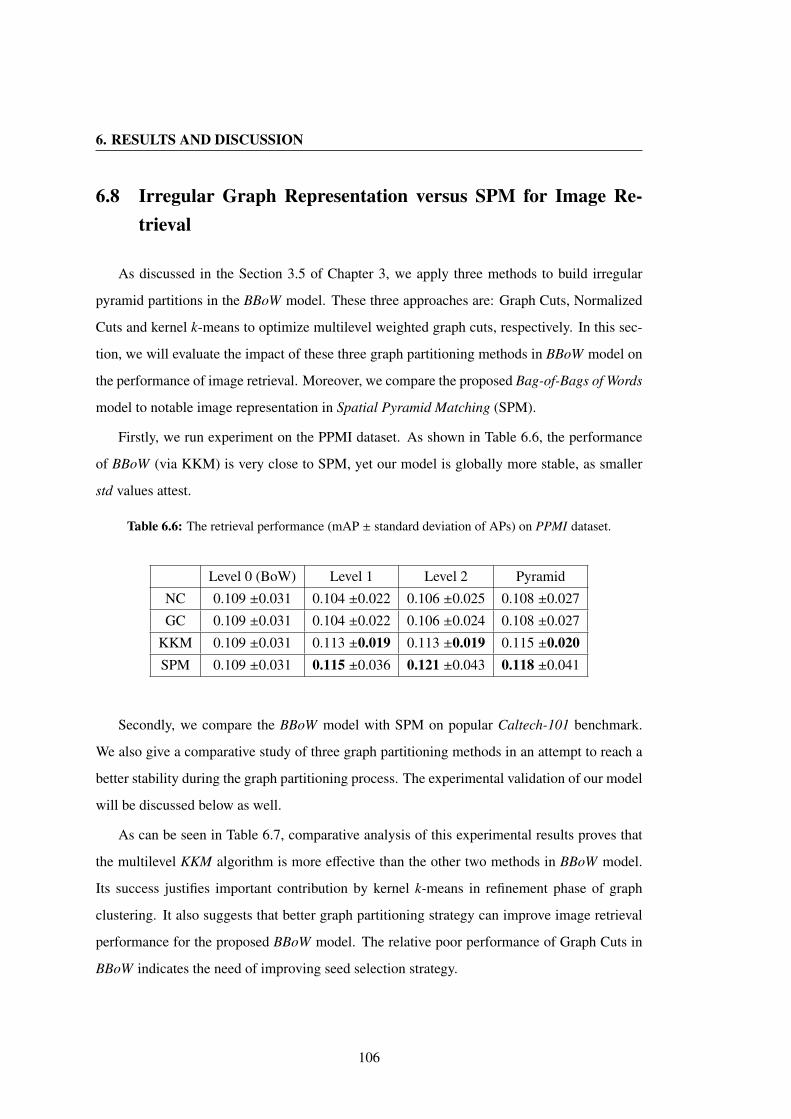
6. RESULTS AND DISCUSSION
6.8 Irregular Graph Representation versus SPM for Image Re-trieval
As discussed in the Section 3.5 of Chapter 3, we apply three methods to build irregular
pyramid partitions in the BBoW model. These three approaches are: Graph Cuts, Normalized
Cuts and kernel k-means to optimize multilevel weighted graph cuts, respectively. In this sec-
tion, we will evaluate the impact of these three graph partitioning methods in BBoW model on
the performance of image retrieval. Moreover, we compare the proposed Bag-of-Bags of Words
model to notable image representation in Spatial Pyramid Matching (SPM).
Firstly, we run experiment on the PPMI dataset. As shown in Table 6.6, the performance
of BBoW (via KKM) is very close to SPM, yet our model is globally more stable, as smaller
std values attest.
Table 6.6: The retrieval performance (mAP ± standard deviation of APs) on PPMI dataset.
Level 0 (BoW) Level 1 Level 2 Pyramid
NC 0.109 ±0.031 0.104 ±0.022 0.106 ±0.025 0.108 ±0.027
GC 0.109 ±0.031 0.104 ±0.022 0.106 ±0.024 0.108 ±0.027
KKM 0.109 ±0.031 0.113 ±0.019 0.113 ±0.019 0.115 ±0.020SPM 0.109 ±0.031 0.115 ±0.036 0.121 ±0.043 0.118 ±0.041
Secondly, we compare the BBoW model with SPM on popular Caltech-101 benchmark.
We also give a comparative study of three graph partitioning methods in an attempt to reach a
better stability during the graph partitioning process. The experimental validation of our model
will be discussed below as well.
As can be seen in Table 6.7, comparative analysis of this experimental results proves that
the multilevel KKM algorithm is more effective than the other two methods in BBoW model.
Its success justifies important contribution by kernel k-means in refinement phase of graph
clustering. It also suggests that better graph partitioning strategy can improve image retrieval
performance for the proposed BBoW model. The relative poor performance of Graph Cuts in
BBoW indicates the need of improving seed selection strategy.
106
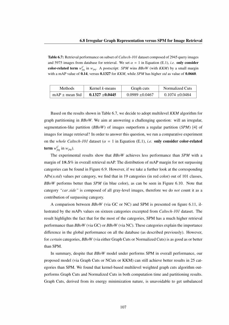
6.8 Irregular Graph Representation versus SPM for Image Retrieval
Table 6.7: Retrieval performance on subset of Caltech-101 dataset composed of 2945 query imagesand 5975 images from database for retrieval. We set α = 1 in Equation (E.1), i.e. only considercolor-related term wC
pq in wpq. A postscript: SPM wins BBoW (with KKM) by a small marginwith a mAP value of 0.14, versus 0.1327 for KKM, while SPM has higher std as value of 0.0660.
Methods Kernel k-means Graph cuts Normalized Cuts
mAP ± mean Std 0.1327 ±0.0445 0.0989 ±0.0467 0.1074 ±0.0484
Based on the results shown in Table 6.7, we decide to adopt multilevel KKM algorithm for
graph partitioning in BBoW. We aim at answering a challenging question: will an irregular,
segmentation-like partition (BBoW) of images outperform a regular partition (SPM) [4] of
images for image retrieval? In order to answer this question, we run a comparative experiment
on the whole Caltech-101 dataset (α = 1 in Equation (E.1), i.e. only consider color-related
term wCpq in wpq).
The experimental results show that BBoW achieves less performance than SPM with a
margin of 18.5% in overall retrieval mAP. The distribution of mAP margin for not surpassing
categories can be found in Figure 6.9. However, if we take a further look at the corresponding
APs(±std) values per category, we find that in 19 categories (in red color) out of 101 classes,
BBoW performs better than SPM (in blue color), as can be seen in Figure 6.10. Note that
category “car side” is composed of all gray-level images, therefore we do not count it as a
contribution of surpassing category.
A comparison between BBoW (via GC or NC) and SPM is presented on figure 6.11, il-
lustrated by the mAPs values on sixteen categories excerpted from Caltech-101 dataset. The
result highlights the fact that for the most of the categories, SPM has a much higher retrieval
performance than BBoW (via GC) or BBoW (via NC). These categories explain the importance
difference in the global performance on all the database (as described previously). However,
for certain categories, BBoW (via either Graph Cuts or Normalized Cuts) is as good as or better
than SPM.
In summary, despite that BBoW model under performs SPM in overall performance, our
proposed model (via Graph Cuts or NCuts or KKM) can still achieve better results in 25 cat-
egories than SPM. We found that kernel-based multilevel weighted graph cuts algorithm out-
performs Graph Cuts and Normalized Cuts in both computation time and partitioning results.
Graph Cuts, derived from its energy minimization nature, is unavoidable to get unbalanced
107

6. RESULTS AND DISCUSSION
Figure 6.9: The margin of mean Average Precision (mAP) for not surpassing categories in Caltech-101 dataset. The margin =
mAP(S PM)−mAP(KKM)mAP(KKM) %.
Figure 6.10: Mean Average Precision for surpassing categories in Caltech-101 dataset.
108
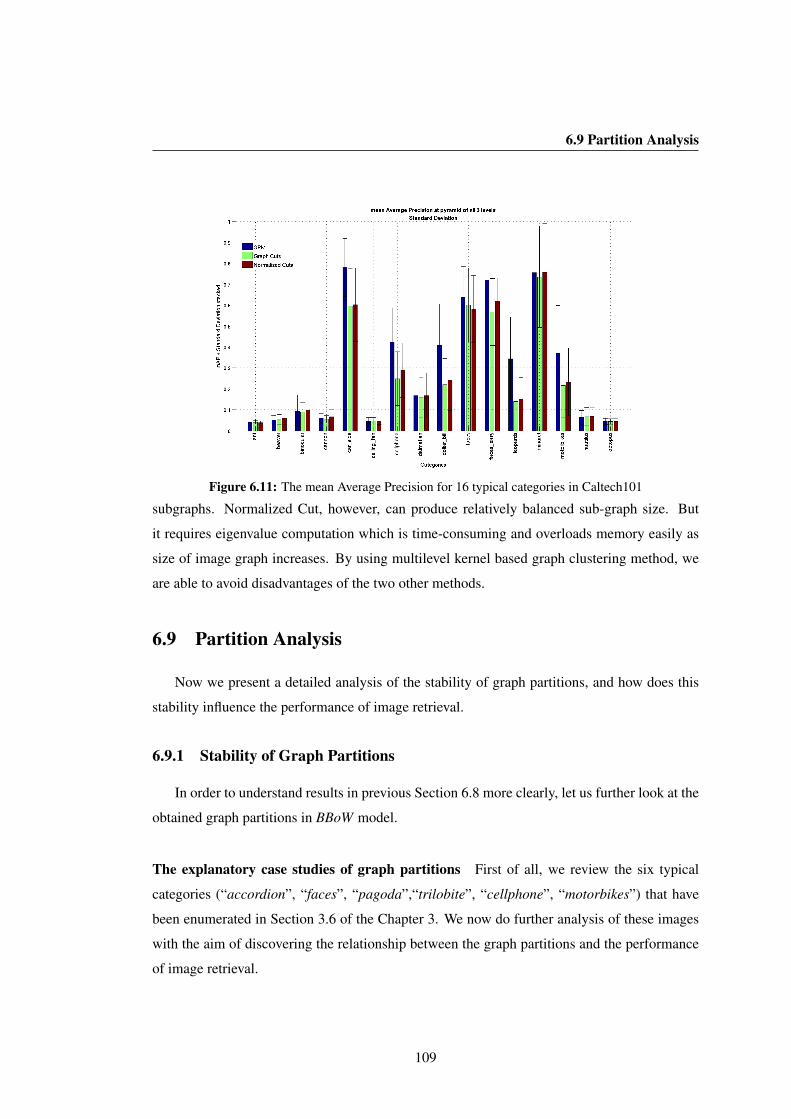
6.9 Partition Analysis
Figure 6.11: The mean Average Precision for 16 typical categories in Caltech101
subgraphs. Normalized Cut, however, can produce relatively balanced sub-graph size. But
it requires eigenvalue computation which is time-consuming and overloads memory easily as
size of image graph increases. By using multilevel kernel based graph clustering method, we
are able to avoid disadvantages of the two other methods.
6.9 Partition Analysis
Now we present a detailed analysis of the stability of graph partitions, and how does this
stability influence the performance of image retrieval.
6.9.1 Stability of Graph Partitions
In order to understand results in previous Section 6.8 more clearly, let us further look at the
obtained graph partitions in BBoW model.
The explanatory case studies of graph partitions First of all, we review the six typical
categories (“accordion”, “faces”, “pagoda”,“trilobite”, “cellphone”, “motorbikes”) that have
been enumerated in Section 3.6 of the Chapter 3. We now do further analysis of these images
with the aim of discovering the relationship between the graph partitions and the performance
of image retrieval.
109

6. RESULTS AND DISCUSSION
Taking each image as a query, retrieval performance was evaluated in mAP on subset of
Caltech-101 dataset composed of 5975 images from database for retrieval. The patch size is
set to n = 5. λ = 5. We here only give a concise evaluation on the case of 4 partitions. The
corresponding mAPs are listed in Table 6.8 resp. Figure 3.12, Table 6.9 resp. Figure 3.13,
Table 6.10 resp. Figure 3.14, Table 6.11 resp. Figure 3.15, Table 6.12 resp. Figure 3.16,
Table 6.13 resp. Figure 3.17 1.
It is shown that our BBoW model clearly outperforms SPM for all examples of images listed
in Figure 3.12, Figure 3.13, Figure 3.14 and Figure 3.15, from four different categories: “ac-
cordion”, “faces”, “pagoda”,“trilobite”. Particularly for the “faces” category, BBoW via KKM
gives the best results. As can be seen on the third column of Figure 3.13, our method is able to
represent the “faces” with only one or two subgraphs. The other subgraphs in the background
are also stable in the sense that almost the same subgraphs can be found in each high-ranking
retrieved image within “faces” category. More details can be referred to the Table B.4 resp.
Figure B.1, Table B.5 resp. Figure B.2, Table B.6 resp. Figure B.3, Table B.7 resp. Figure B.4,
Table B.8 resp. Figure B.5 in Appendix B. The same case holds in category “trilobite”, where
BBoW via Normalized Cut surpasses SPM. The second column of Figure 3.15 presents the
partitioning results on five images from the “trilobite” category. Once again, it can be observed
that the partitions are stable.
Figure 3.16 and Figure 3.17 on the other hand represents two categories (“cellphone” and
“motorbikes”) for which our method fails. The partitions obtained almost do not exhibit any
consistency across the images from the same category. The resulting histograms are therefore
each time very different. Obviously, we cannot expect any good retrieval.
The statistical analysis of subgraphs In order to give a deeper understanding on why our
method suits for certain categories and not for the others, let us go through again the other three
case studies: a “good” category (“minaret”), and two “bad” ones (“cellphone”, “dollar bill”).
Figure 6.12 presents the partitioning results at level 1, i.e. 4 subgraphs. The first row
of the Figure 6.12 illustrates good queries from “minaret” class in which BBoW outperforms
SPM. Once again, our method is able to represent the “minaret” (object) with only one or two
subgraph(s). The other subgraphs in the background are also stable.
1The file extension of each image is omitted in these Tables and Figures. The highest value of mAPs is shownin bold for each query image.
110

6.9 Partition Analysis
Table 6.8: The comparison of mAPs for BBoW (via GC) vs BBoW (via NCuts) vs BBoW (viaKKM) vs SPM on 4 partitions of five examples of images from category “accordion”. See Fig-ure 3.12.
Image GC NCuts KKM SPM
accordion0031 0.3439 0.6328 0.5835 0.0718
accordion0032 0.6238 0.6047 0.5994 0.3693
accordion0041 0.7535 0.6080 0.6401 0.4414
accordion0053 0.4886 0.6382 0.5673 0.2957
accordion0055 0.7175 0.6119 0.6211 0.1909
Table 6.9: The comparison of mAPs for BBoW (via GC) vs BBoW (via NCuts) vs BBoW (viaKKM) vs SPM on 4 partitions of five examples of images from category “faces”. See Figure 3.13.
Image GC NCuts KKM SPM
faces0032 0.6979 0.6729 0.9086 0.5949
faces0036 0.6431 0.5716 0.9146 0.5139
faces0038 0.6240 0.4250 0.9314 0.4991
faces0039 0.5938 0.6098 0.9042 0.6094
faces0049 0.5453 0.4881 0.9091 0.5404
Table 6.10: The comparison of mAPs for BBoW (via GC) vs BBoW (via NCuts) vs BBoW (viaKKM) vs SPM on 4 partitions of five examples of images from category “pagoda”. See Figure 3.14.
Image GC NCuts KKM SPM
pagoda0035 0.2647 0.3246 0.6960 0.5297
pagoda0040 0.5955 0.5449 0.6894 0.6722
pagoda0043 0.8271 0.3784 0.7534 0.6794
pagoda0046 0.4102 0.5622 0.7596 0.7169
pagoda0047 0.6674 0.4556 0.7185 0.5542
The second row of the Figure 6.12 shows four bad queries from cellphone and dollar bill
categories in which SPM achieves better performance than our method. We have the same
111

6. RESULTS AND DISCUSSION
Table 6.11: The comparison of mAPs for BBoW (via GC) vs BBoW (via NCuts) vs BBoW (viaKKM) vs SPM on 4 partitions of five examples of images from category “trilobite”. See Fig-ure 3.15.
Image GC NCuts KKM SPM
trilobite0037 0.5975 0.7040 0.6342 0.4386
trilobite0041 0.3561 0.6575 0.6612 0.5174
trilobite0056 0.6229 0.8055 0.6550 0.5787
trilobite0064 0.3551 0.6805 0.6645 0.5087
trilobite0072 0.6823 0.8540 0.6186 0.2240
Table 6.12: The comparison of mAPs for BBoW (via GC) vs BBoW (via NCuts) vs BBoW (viaKKM) vs SPM on 4 partitions of five examples of images from category “cellphone”. See Fig-ure 3.16.
Image GC NCuts KKM SPM
cellphone0032 0.2372 0.2439 0.1448 0.3429cellphone0035 0.1742 0.0567 0.1018 0.3215cellphone0049 0.1153 0.1832 0.1197 0.3117cellphone0051 0.2644 0.5100 0.3845 0.7288cellphone0059 0.2768 0.3254 0.2098 0.3637
Table 6.13: The comparison of mAPs for BBoW (via GC) vs BBoW (via NCuts) vs BBoW (viaKKM) vs SPM on 4 partitions of five examples of images from category “motorbikes”. See Fig-ure 3.17.
Image GC NCuts KKM SPM
motorbikes0042 0.3622 0.2407 0.2347 0.4885motorbikes0043 0.4249 0.2950 0.2308 0.5262motorbikes0047 0.3024 0.2630 0.1998 0.5967motorbikes0055 0.3668 0.2704 0.1691 0.4293motorbikes0059 0.3943 0.1734 0.3839 0.5856
112
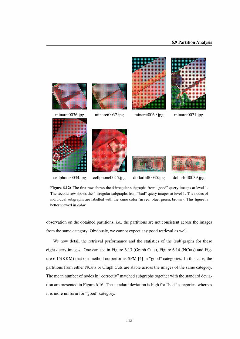
6.9 Partition Analysis
minaret0036.jpg minaret0037.jpg minaret0069.jpg minaret0071.jpg
cellphone0034.jpg cellphone0045.jpg dollarbill0035.jpg dollarbill0039.jpg
Figure 6.12: The first row shows the 4 irregular subgraphs from “good” query images at level 1.The second row shows the 4 irregular subgraphs from “bad” query images at level 1. The nodes ofindividual subgraphs are labelled with the same color (in red, blue, green, brown). This figure isbetter viewed in color.
observation on the obtained partitions, i.e., the partitions are not consistent across the images
from the same category. Obviously, we cannot expect any good retrieval as well.
We now detail the retrieval performance and the statistics of the (sub)graphs for these
eight query images. One can see in Figure 6.13 (Graph Cuts), Figure 6.14 (NCuts) and Fig-
ure 6.15(KKM) that our method outperforms SPM [4] in “good” categories. In this case, the
partitions from either NCuts or Graph Cuts are stable across the images of the same category.
The mean number of nodes in “correctly” matched subgraphs together with the standard devia-
tion are presented in Figure 6.16. The standard deviation is high for “bad” categories, whereas
it is more uniform for “good” category.
113

6. RESULTS AND DISCUSSION
Figure 6.13: A case study of BBoW (via Normalized Cuts). The precision of 8 typical queryimages: 1st-4th query images are from a “good” category - minaret, 5th-8th query images arefrom “bad” categories: cellphone and dollar bill.
6.9.2 Quality of Subgraphs Matching
To access subgraphs matching, we use the partition precision introduced in Section 6.3.2.
The partition precision (PP) of 4 subgraphs for 8 typical queries (|η| = 30) are shown in ta-
ble 6.14 and table 6.15. We find that in “good” categories, the Precision(Γkj) for each subgraph
g j,k is close to 1, signifies that the subgraphs are matched correctly more often. That illustrates
the discriminative power of graph descriptors among inter-class. While P(Γkj)k=1,...,4 are high,
it means the image graph partitions tend to be more stable. In “bad” categories, this happens
less often.
In the context of intra-category, the Partition Precision (PP) for query image I j is thus
given by a row vector of length K:
P(g j,k)k=1, ..., K =1|Nrel|
∑d=1...|Nrel |
Md,k (6.11)
where Md,k is an element of matrix M. The above vector thus characterizes the goodness of
match of each subgraph in a query image to the subgraphs of images of the same category in
114

6.9 Partition Analysis
Figure 6.14: A case study of BBoW (via Graph Cuts). The precision of 8 typical query images:1st-4th query images are from a “good” category - minaret, 5th-8th query images are from “bad”categories: cellphone and dollar bill.
Table 6.14: The PP Precision(Γkj)k=1,2,3,4 = P(g j,k)k=1,2,3,4 of corresponding subgraphs for 4
typical “good” queries. Method: BBoW via Normalized Cut.
Query image I j g j,1 g j,2 g j,3 g j,4
minaret0036 0.933 0.867 0.833 0.867minaret0037 1.0 0.9 0.833 0.933minaret0069 1.0 0.967 0.9 1.0minaret0071 0.967 0.9 0.833 0.8
the database Ω. Table 6.18 and 6.19 show figures for the partition precision of 4 typical queries
of a “good” category and of two “bad” categories. The corresponding number of nodes for each
subgraph, as illustrated in Figure 6.16, is also listed in Table 6.16 and Table 6.17 respectively
in detail. Note that in Table 6.17, the standard deviation on a number of nodes is generally
larger than that one in Table 6.16.
In Table 6.18, one can see that in the “good” categories, the worst matching percentage
(the numbers in bold) is better than that in “bad” queries. Hence, this correlates with better
115

6. RESULTS AND DISCUSSION
Figure 6.15: A case study of BBoW (via Kernel k-means). The precision of 8 typical queryimages: 1st-4th query images are from a “good” category - minaret, 5th-8th query images arefrom “bad” categories: cellphone and dollar bill.
Table 6.15: The PP Precision(Γkj)k=1,2,3,4 = P(g j,k)k=1,2,3,4 of corresponding subgraphs for 4
typical “bad” queries. Method: BBoW via Normalized Cut.
Query image I j g j,1 g j,2 g j,3 g j,4
cellphone0034 0.433 0.467 0.3 0.433cellphone0045 0.3 0.3 0.267 0.267dollar bill0035 0.133 0.2 0.167 0.133dollar bill0039 0.133 0.233 0.133 0.2
stability of nodes’ numbers, as in Figure 6.16, where the number of nodes within the matched
subgraphs is quite imbalance in the “bad” categories.
116

6.9 Partition Analysis
Figure 6.16: The mean and standard deviation of nodes’ numbers of corresponding subgraphsfor intra-category, for 8 typical queries in Caltech-101 dataset - at single level 1, i.e. 4 subgraphs.
Table 6.16: The mean of node numbers and its standard deviation for corresponding matchedsubgraphs of intra-category minaret, for 4 typical good queries in Caltech-101 dataset, at singlelevel 1, i.e. 4 subgraphs. Method: BBoW via Normalized Cut.
I j Precision g j,1 g j,2 g j,3 g j,4
minaret0036 0.7864 433 ±180 99 ±38 145 ±88 228 ±148minaret0037 0.8694 307 ±185 105 ±70 168 ±116 326 ±207minaret0069 0.8699 419 ±196 123 ±73 123 ±79 243 ±147minaret0071 0.9252 228 ±153 113 ±58 202 ±157 365 ±217
Table 6.17: The mean of node numbers and its standard deviation for corresponding matchedsubgraphs of intra-category cellphone and dollar bill, for 4 typical bad queries in Caltech-101dataset, at single level 1, i.e. 4 subgraphs. Method: BBoW via Normalized Cut.
I j Precision g j,1 g j,2 g j,3 g j,4
cellphone0034 0.4412 703 ±239 82 ±73 157 ±147 43 ±43cellphone0045 0.4576 703 ±233 96 ±97 80 ±97 104 ±111dollar bill0035 0.1263 164 ±111 72 ±83 34 ±50 355 ±132dollar bill0039 0.1540 374 ±111 123 ±94 74 ±78 53 ±63
117

6. RESULTS AND DISCUSSION
Table 6.18: The P(g j,k)k=1,...,4 of corresponding subgraphs for 4 typical “good” queries. Method:BBoW via Normalized Cut.
Query image I j g j,1 g j,2 g j,3 g j,4
minaret0036 0.773 0.746 0.626 0.6minaret0037 0.786 0.72 0.626 0.6minaret0069 0.773 0.44 0.6 0.613minaret0071 0.8 0.506 0.6 0.413
Table 6.19: The P(g j,k)k=1,...,4 of corresponding subgraphs for 4 typical “bad” queries. Method:BBoW via Normalized Cut.
Query image I j g j,1 g j,2 g j,3 g j,4
cellphone0034 0.724 0.638 0.569 0.241cellphone0045 0.724 0.362 0.569 0.552dollar bill0035 0.431 0.686 0.392 0.176dollar bill0039 0.275 0.824 0.06 0.418
6.10 Conclusion
In this Chapter, we provided our experimental results on three image benchmarks, to val-
idate the proposed BBoW model. We also compared BBoW with a notable approach spatial
pyramid matching. As compared with Spatial Pyramid Matching (SPM), the BBoW model
overcomes the practical limitations of assuming similar parts of scenes very often appear in
similar regular grid cells. Particularly, we emphasize that the partitions in BBoW are not nested
across multiple levels.
We also gave an analysis of the images sampled from four “good” categories and two
“bad” categories in Caltech-101 dataset, as case studies to reveal the relationship between the
stability of graph partitions and the performance of image retrieval. We have found: despite
that the BBoW model does not perform as good as SPM overall, the strength of our method
is promising for image retrieval when the partitions are stable across an image category, e.g.
“accordion”, “faces”, “pagoda”, “trilobite” categories in Caltech-101 dataset, see Section 6.9.1
and Appendix B for reference. The experiments demonstrate that our proposed method is
globally more stable and performs better than SPM in 19 objects categories.
118
Chapter 7
Conclusion and Perspectives
In this chapter, we will summarize the contributions made in the present work and then
enumerate possible directions for the future research.
7.1 Summary of the Work in this Dissertation
In this thesis, we have proposed a novel model as a way of graph-based image represen-
tation, namely Bag-of-Bags of Words (BBoW), to incorporate both the appearance and spatial
information under its description. Basically, BBoW is a bag of signatures, each of which is
built on a subgraph in image. The construction of BBoW model is composed of four steps:
1) Local features extraction; 2) Image graph construction; 3) Irregular subgraphs generation;
and 4) BBoW description. The BBoW description is a combination of a bag of signatures. Each
signature is built on a subgraph in the image.
In the process of graph construction, we mainly adopted two approaches: 1) prominent
keypoints; 2) dense sampling for graph nodes selection. We have also designed several ob-
jective functions to define the weights of edges in the image graph. These objective functions
are related to either color information or texture features of graph nodes, and they may com-
bine both of them as well, i.e. like joint color-texture descriptors. Furthermore, we formulated
different types of edge-weight terms, then analysed their influences on the stability of image
graph partitioning in the following step.
We then evaluated three graph partitioning methods: Graph Cuts, Normalized Cuts and
kernel k-means to optimize multilevel weighted graph cuts (KKM), for irregular image partition
in the third step. A criterion for measuring the stability of subgraphs has been defined. It has
119

7. CONCLUSION AND PERSPECTIVES
been shown that KKM approach achieved better result than the other two partitioning methods.
This finding suggests that better graph partitioning strategy can improve the performance for
the BBoW model.
In BBoW model, each subgraph is described by a bag-of-visual-words histogram as its
signature. An image is thus represented by concatenating those signatures together with level
weighted normalizations. For matching BBoWs, a crucial technique, called bipartite subgraphs
matching was used. With this technique, the BBoW achieves spatial invariance in image repre-
sentation.
In contrast to the state-of-the-art technique such as Fisher vector image representation [20,
21, 99] and spatially local coding [102] etc. that compete with SPM to give extensions of bag-
of-words image representations to encode spatial layout, our model takes into account spatial
constraints in the image space instead of feature space. Our approach incorporates color and
limited spatial information into image representation for image retrieval.
Finally, we validated the BBoW model for a given task of image retrieval in three datasets
(SIVAL, PPMI, Caltech-101) with a total of 13, 044 images. The obtained results are encour-
aging, especially when the obtained partitions are stable across the images from the same cat-
egory. The experiments on one of the most well-known benchmark Caltech-101 demonstrate
that applying kernel k-means to graph clustering process produces better image retrieval re-
sults, as compared with other graph partitioning methods such as Graph Cuts and Normalized
Cuts for BBoW model. Moreover, this proposed method achieves comparable results and out-
performs SPM in 19 object categories on the whole Caltech-101 dataset.
To formally evaluate the performance of the model, we have introduced a new vector fea-
tures: partition precision. It characterizes the quality of matching of each subgraph in the
image graph. Scalar metrics could be induced from partition precision, but require a thorough
study of their properties. We formalized the model, proposed the methodological chain for its
construction in images, developed a comparison methodology for matching images by BBoW
in a CBIR framework.
We have further extended the model to its pyramidal extension, where a non-nested multi-
levels scheme of image partitions was proposed. The irregular partitions at each level are
independent of those at other level(s). An image represented by a pyramid of fixed number
of partitions is described by a bottom-up reordered collection of BBoW for all levels. The
matching of these descriptions has been called irregular pyramid matching (IPM).
120

7.2 Future Work
7.2 Future Work
As future work, we consider defining an information fusion scheme based on the “verti-
cal” property across multiple resolutions of image graph partitions, and applying a multi-class
classifier to the proposed BBoW model for image classification. Adding more discriminative
texture features in BBoW, in addition to studying effective ways to embed texture information
is another interesting direction. A comparison to state-of-the-art algorithms like deep learn-
ing [162, 163] would obviously be important to carry on in the future.
In summary, we plan to improve and extend our BBoW model mainly in the following four
directions:
7.2.1 Objective Functions in Edges Weights
As discussed in Section 6.9 of Chapter 6, the stability of graph partitions is nevertheless
not always ensured with the predefined functions for edge weights. To improve this stability,
we plan to use other objective functions for edge weights in graph partitioning methods. We
also aim to test other discriminative texture features, such as Local binary patterns (LBP) [48]
and Multi-factal spectrum (MFS) [164, 165], then study different ways to combine color and
texture features in edge weights.
7.2.2 Improving Segmentation Methods
The BBoW model can potentially adopt any automatic image segmentation methods com-
bined with the bag-of-words model. With such extensions, many interesting options remain to
be explored.
For example, in the context of Graph Cuts, we can adaptively change the regularization
parameter λ, as justified in Candemir et al. [166]: using adaptive regularization parameters
for the different parts of the image improves the segmentation result than using a single reg-
ularization parameter. The proposed method adjusts the effect of the regularization parameter
using the probabilities of pixels being part of the boundary. Intuitively, it can produce better
segmentation results than the original graph cut approach for the best λ.
7.2.3 Fusion across Graph Partitions
Agarwal et al. [19] proposed a multilevel local coding method called “hyperfeatures”,
which are ”features of (local sets of) features (from lower level)”. This approach is based
121

7. CONCLUSION AND PERSPECTIVES
on local histogram model encoding co-occurrence statistics within each local neighbourhood
at multilevel. The level 0 (base level) contains bag of features (BoF) histograms, i.e. global
histograms over quantized image descriptors. The higher level consists of local histograms
generated by repeatedly aggregating local BoF histograms from previous lower level features.
The codebook of hyperfeatures is learned from all features at the corresponding level during
training.
In contrast, current implementation of BBoW model does not feed lower level features
into the computational process of higher levels. At each resolution of the image partitions,
subgraphs are built independently on single level basis. The BoW approach is next applied to
individual resulting subgraphs independently as well. That is to say, the signatures (histograms)
of (sub)graphs are independent of the resolutions of image partitions. Moreover, the codebook
in BBoW is independent from any partitioning scheme. Inspired by “hyperfeatures”, we may
as well build our “hyperfeatures” in BBoW by the fusion of features across graph partitions.
7.2.4 Applications of the BBoW Model
From a more fundamental point of view, there are some other aspects of the proposed
model that we are interested in tackling in the future. First of all, we are interested to see
how robust our model is against noisy data. Secondly, we intend to further develop statistical
analysis of subgraphs in order to interpret these graph descriptors (subgraphs) and to study
further their stability with respect to graph partitioning. Thirdly, many distance metrics and
similarity functions can be applied to define similarity measures for comparing the images.
From an applicative point of view, we aim to validate the generality of this model on wide
range of data sets for tasks of object image classification and scene classification. Another
applicative foreseen work is to apply BBoW to images with large resolutions, as the graph
descriptors can be more representative in terms of larger image space.
122

Appendix A
Experimental Results in SIVAL
Bag-of-Bags of Visual Word (BBoVW) versus Bag-of-Visual Words (BoVW) in SIVAL dataset
In this Appendix, we enumerate experimental results in SIVAL dataset. In Figure A.1,
BoVW and BBoW are compared. Figure A.2 demonstrates the impact of different co-occurrence
criteria (see Section 4.3.1) on the performance of image retrieval. More details can also be re-
ferred in Table A.1. An the end of the appendix, we list the category-based Precision-Recall
curve for 25 categories in SIVAL dataset.
123

A. EXPERIMENTAL RESULTS IN SIVAL
Figure A.1: The overall Precision-Recall curve for a comparison between BBoVW and BoVWin SIVAL dataset [10]. BBoVW: Bag-of-Bags of Visual Word. BoVW: Bag-of-Visual Words.Each image is composed of 4 subgraphs in BBoW. The dictionary of size 1000, as described inSection 6.2.1 of the Chapter 6, is learnt over 30 sample images per class using k-means. The queryimages are chosen from the rest of the SIVAL dataset for retrieval. In this figure, the red curvecorresponds to application of co-occurrence measure defined in Equation (4.4) for image matchingin the BBoW Model. The blue/red curve correspond to BoVW with/without points filtration.
124
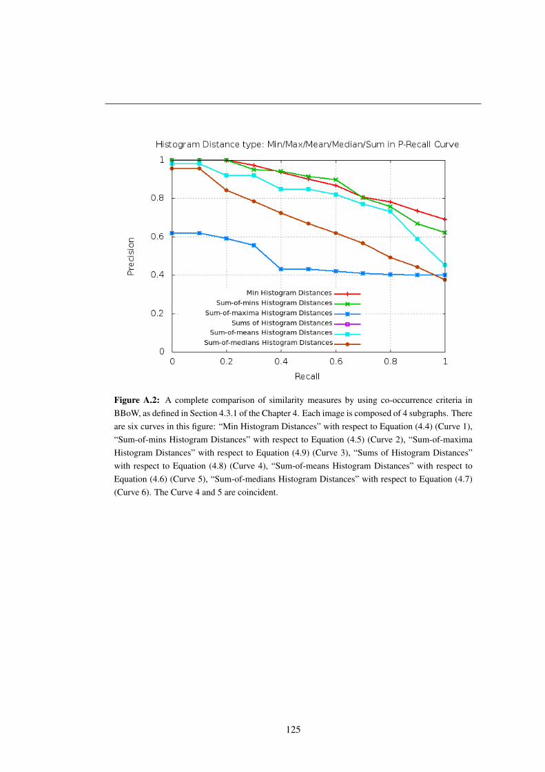
Figure A.2: A complete comparison of similarity measures by using co-occurrence criteria inBBoW, as defined in Section 4.3.1 of the Chapter 4. Each image is composed of 4 subgraphs. Thereare six curves in this figure: “Min Histogram Distances” with respect to Equation (4.4) (Curve 1),“Sum-of-mins Histogram Distances” with respect to Equation (4.5) (Curve 2), “Sum-of-maximaHistogram Distances” with respect to Equation (4.9) (Curve 3), “Sums of Histogram Distances”with respect to Equation (4.8) (Curve 4), “Sum-of-means Histogram Distances” with respect toEquation (4.6) (Curve 5), “Sum-of-medians Histogram Distances” with respect to Equation (4.7)(Curve 6). The Curve 4 and 5 are coincident.
125

A. EXPERIMENTAL RESULTS IN SIVAL
Table A.1: The precision-recall values of experimental results, as complementary informationof Figure A.2. The experiments were run in SIVAL dataset with the aim of comparing a seriesof similarity measures (co-occurrence criteria) versus the classical bag-of-words model for imageretrieval. The fist column lists recall values ranging from 0 to 1.0 of 11 intervals. The 2nd-8thcolumns correspond to the precision values for seven different measures. They are (1) Bag-of-Words (BoW), without filtering points in graph nodes selection; (2) BoW, select graph nodes bypoints filtration; (3) Bag-of-Bag-of-Visual-Words (BBoVW), using Equation (4.4); (4) BBoVW,using Equation (4.5); (5) BBoVW, using Equation (4.6) or its equivalent by using Equation (4.8);(6) BBoVW, using Equation (4.7); (7) BBoVW, using Equation (4.9) respectively.
Recall BoW(withpointsfiltra-tion)
BoW(sanspointsfiltra-tion)
BBoVW(min)
BBoVW(sum-of-
min)
BBoVW(mean)(sum)
BBoVW(median)
BBoVW(max)
0 0.6077 1.0000 1.0000 1.0000 0.9794 0.9571 0.6180
0.1 0.6077 1.0000 1.0000 1.0000 0.9794 0.9571 0.6180
0.2 0.5854 0.9722 1.0000 1.0000 0.9198 0.8430 0.5914
0.3 0.5699 0.9356 0.9722 0.9500 0.9198 0.7832 0.5545
0.4 0.5699 0.9007 0.9356 0.9426 0.8489 0.7246 0.4319
0.5 0.5625 0.8667 0.9007 0.9136 0.8489 0.6687 0.4299
0.6 0.5393 0.8077 0.8667 0.8966 0.8217 0.6201 0.4193
0.7 0.5289 0.7815 0.8077 0.8039 0.7695 0.5659 0.4079
0.8 0.5039 0.7345 0.7815 0.7562 0.7330 0.4910 0.4026
0.9 0.4606 0.6910 0.7345 0.6690 0.5875 0.4421 0.4008
1.0 0.4441 0.6270 0.6910 0.6203 0.4543 0.3765 0.4008
126

(1) “ajaxorange” (2) “apple” (3) “banana”
(4) “bluescrunge” (5) “candlewithholder” (6) “cardboardbox”
(7) “checkeredscarf” (8) “cokecan” (9) “dataminingbook”
(10) “dirtyrunningshoe” (11) “dirtyworkgloves” (12) “fabricsoftenerbox”
(13) “feltflowerrug” (14) “glazedwoodpot” (15) “goldmedal”Figure is continued on next page
127

A. EXPERIMENTAL RESULTS IN SIVAL
(16) “greenteabox” (17) “juliespot” (18) “largespoon”
(19) “rapbook” (20) “smileyfacedoll” (21) “spritecan”
(22) “stripednotebook” (23) “translucentbowl” (24) “wd40can”
(25) “woodrollingpin”
Figure A.3: The category-based Precision-Recall curve for 25 categories in SIVAL dataset.
128

Appendix B
Experimental Results in Caltech-101
Irregular partition versus regular partition (4 partitions) in Caltech-101 dataset
In this Appendix, we enumerate experimental results in Caltech-101 dataset [144]. Firstly,
we provide a thorough comparison between BBoW via KKM and SPM at single level 1, i.e.,
4 partitions per image. The category-based average precisions (APs) and their corresponding
standard deviation (Std) are given in Table B.1. Secondly, we list global retrieval performance
of BBoW via KKM (see Table B.2), BBoW via Graph Cuts, BBoW via Normalized Cut, vs
SPM (see Table B.3) in Caltech-101 dataset. Thirdly, we give a case study in “faces” category,
on five image samples: face0032.jpg, face0036.jpg, face0038.jpg, face0039.jpg, face0049.jpg.
The retrieval result of these images can be referred in Table B.8, Table B.8, Table B.8, Table B.8
and Table B.8. The twenty high-ranking retrieved images are shown in Figure B.1, Figure B.2,
Figure B.3, Figure B.4 and Figure B.5 respectively. The Figure B.6 at the end of the Appendix
demonstrates the distribution of average precision values of image retrieval from 20 surpassing
classes on the whole Caltech-101 dataset, which corresponds to the comparison between SPM
and BBoW (via KKM) in Figure 6.10 of Chapter 6.
129
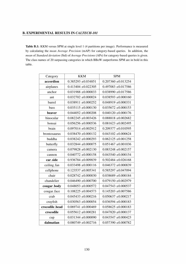
B. EXPERIMENTAL RESULTS IN CALTECH-101
Table B.1: KKM versus SPM at single level 1 (4 partitions per image). Performance is measuredby calculating the mean Average Precision (mAP) for category-based queries. In addition, themean of Standard deviation (Std) of Average Precisions (APs) for category-based queries is given.The class names of 20 surpassing categories in which BBoW outperforms SPM are in bold in thistable.
Category KKM SPM
accordion 0.385293 ±0.034851 0.207360 ±0.013254
airplanes 0.413404 ±0.022305 0.497083 ±0.017586
anchor 0.031988 ±0.000033 0.038990 ±0.017586
ant 0.032702 ±0.000024 0.038593 ±0.000160
barrel 0.038911 ±0.000252 0.048919 ±0.000331
bass 0.035115 ±0.000130 0.035672 ±0.000153
beaver 0.044052 ±0.000208 0.040120 ±0.000176
binocular 0.082245 ±0.003426 0.088818 ±0.002682
bonsai 0.056256 ±0.000536 0.081623 ±0.002495
brain 0.097014 ±0.002912 0.209377 ±0.010595
brontosaurus 0.038470 ±0.000132 0.043102 ±0.000624
buddha 0.038242 ±0.000293 0.062125 ±0.001258
butterfly 0.032844 ±0.000075 0.051467 ±0.001036
camera 0.079828 ±0.002130 0.083248 ±0.002157
cannon 0.040772 ±0.000158 0.043540 ±0.000154
car side 0.936784 ±0.009839 0.502484 ±0.026168
ceiling fan 0.033498 ±0.000116 0.046372 ±0.000839
cellphone 0.123537 ±0.005341 0.585297 ±0.047094
chair 0.028742 ±0.000030 0.038689 ±0.000184
chandelier 0.046490 ±0.000700 0.079150 ±0.002979
cougar body 0.048053 ±0.000572 0.047543 ±0.000537
cougar face 0.108225 ±0.004573 0.145203 ±0.007586
crab 0.045433 ±0.000216 0.050637 ±0.000217
crayfish 0.030563 ±0.000054 0.036594 ±0.000183
crocodile head 0.069741 ±0.000469 0.058625 ±0.000183
crocodile 0.055612 ±0.000281 0.047820 ±0.000137
cup 0.031344 ±0.000090 0.043547 ±0.000423
dalmatian 0.080749 ±0.002716 0.057390 ±0.000782
130
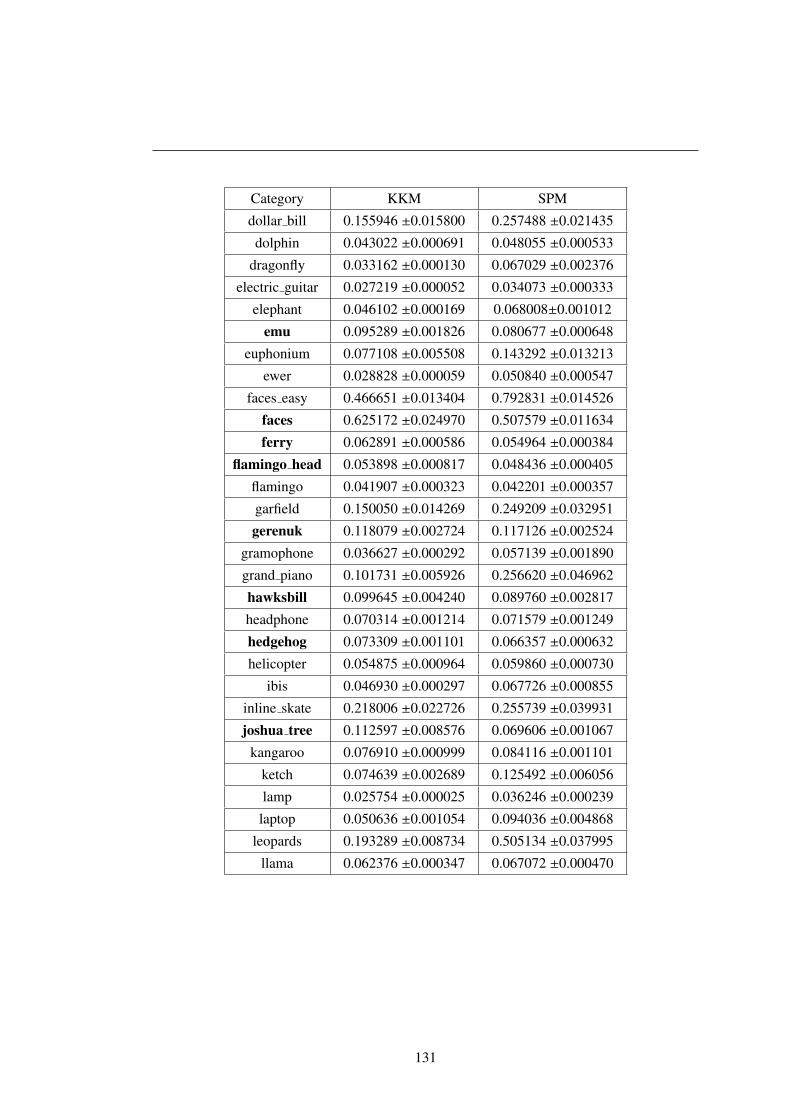
Category KKM SPM
dollar bill 0.155946 ±0.015800 0.257488 ±0.021435
dolphin 0.043022 ±0.000691 0.048055 ±0.000533
dragonfly 0.033162 ±0.000130 0.067029 ±0.002376
electric guitar 0.027219 ±0.000052 0.034073 ±0.000333
elephant 0.046102 ±0.000169 0.068008±0.001012
emu 0.095289 ±0.001826 0.080677 ±0.000648
euphonium 0.077108 ±0.005508 0.143292 ±0.013213
ewer 0.028828 ±0.000059 0.050840 ±0.000547
faces easy 0.466651 ±0.013404 0.792831 ±0.014526
faces 0.625172 ±0.024970 0.507579 ±0.011634
ferry 0.062891 ±0.000586 0.054964 ±0.000384
flamingo head 0.053898 ±0.000817 0.048436 ±0.000405
flamingo 0.041907 ±0.000323 0.042201 ±0.000357
garfield 0.150050 ±0.014269 0.249209 ±0.032951
gerenuk 0.118079 ±0.002724 0.117126 ±0.002524
gramophone 0.036627 ±0.000292 0.057139 ±0.001890
grand piano 0.101731 ±0.005926 0.256620 ±0.046962
hawksbill 0.099645 ±0.004240 0.089760 ±0.002817
headphone 0.070314 ±0.001214 0.071579 ±0.001249
hedgehog 0.073309 ±0.001101 0.066357 ±0.000632
helicopter 0.054875 ±0.000964 0.059860 ±0.000730
ibis 0.046930 ±0.000297 0.067726 ±0.000855
inline skate 0.218006 ±0.022726 0.255739 ±0.039931
joshua tree 0.112597 ±0.008576 0.069606 ±0.001067
kangaroo 0.076910 ±0.000999 0.084116 ±0.001101
ketch 0.074639 ±0.002689 0.125492 ±0.006056
lamp 0.025754 ±0.000025 0.036246 ±0.000239
laptop 0.050636 ±0.001054 0.094036 ±0.004868
leopards 0.193289 ±0.008734 0.505134 ±0.037995
llama 0.062376 ±0.000347 0.067072 ±0.000470
131

B. EXPERIMENTAL RESULTS IN CALTECH-101
Category KKM SPM
lobster 0.038376 ±0.000053 0.046944 ±0.000315
lotus 0.057295 ±0.001080 0.084398 ±0.003726
mandolin 0.034653 ±0.000181 0.051805 ±0.001065
mayfly 0.038675 ±0.000191 0.033540 ±0.000060
menorah 0.042762 ±0.000631 0.111245 ±0.011053
metronome 0.146016 ±0.017831 0.248172 ±0.035696
minaret 0.563488 ±0.065599 0.761386 ±0.036978
motorbikes 0.346897 ±0.029450 0.484363 ±0.024733
nautilus 0.044776 ±0.000464 0.058587 ±0.000915
octopus 0.061111 ±0.002890 0.065611 ±0.002946
okapi 0.067656 ±0.000787 0.072923 ±0.000662
pagoda 0.513619 ±0.036199 0.425830 ±0.041670
panda 0.053463 ±0.000800 0.090087 ±0.004122
pigeon 0.039460 ±0.000170 0.073331 ±0.004327
pizza 0.060974 ±0.000669 0.119683 ±0.003788
platypus 0.049821 ±0.000454 0.058274 ±0.001475
pyramid 0.037786 ±0.000275 0.047032 ±0.000553
revolver 0.041841 ±0.000527 0.139438 ±0.014844
rhino 0.053988 ±0.000427 0.070488 ±0.000643
rooster 0.038159 ±0.000067 0.070629 ±0.002187
saxophone 0.051035 ±0.000975 0.056405 ±0.002127
schooner 0.051375 ±0.000954 0.108890 ±0.004279
scissors 0.067095 ±0.001286 0.072949 ±0.002014
scorpion 0.048849 ±0.000461 0.054160 ±0.000542
sea horse 0.052618 ±0.000627 0.045046 ±0.000303
snoopy 0.105323 ±0.003779 0.153791 ±0.007804
soccer ball 0.066348 ±0.001613 0.167095 ±0.014295
stapler 0.071884 ±0.002658 0.176760 ±0.017047
starfish 0.057088 ±0.000645 0.078110 ±0.001997
stegosaurus 0.049275 ±0.000891 0.059037 ±0.001392
stop sign 0.094728 ±0.007429 0.181281 ±0.028480
strawberry 0.054906 ±0.000795 0.075049 ±0.002515
sunflower 0.057008 ±0.000710 0.118955 ±0.007903
132
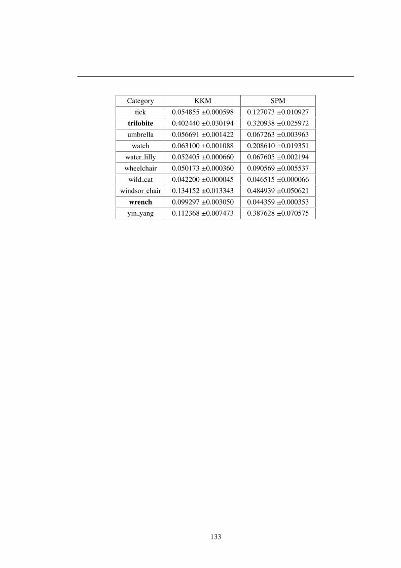
Category KKM SPM
tick 0.054855 ±0.000598 0.127073 ±0.010927
trilobite 0.402440 ±0.030194 0.320938 ±0.025972
umbrella 0.056691 ±0.001422 0.067263 ±0.003963
watch 0.063100 ±0.001088 0.208610 ±0.019351
water lilly 0.052405 ±0.000660 0.067605 ±0.002194
wheelchair 0.050173 ±0.000360 0.090569 ±0.005537
wild cat 0.042200 ±0.000045 0.046515 ±0.000066
windsor chair 0.134152 ±0.013343 0.484939 ±0.050621
wrench 0.099297 ±0.003050 0.044359 ±0.000353
yin yang 0.112368 ±0.007473 0.387628 ±0.070575
133

B. EXPERIMENTAL RESULTS IN CALTECH-101
Table B.2: Evaluation of BBoW via KKM in Caltech-101 dataset. Retrieval performance wasevaluated in mean Average Precision (mAP) on subset of Caltech-101 dataset composed of 2945query images and 5975 images from database for retrieval. The size of codebook is 400.
BBoW via KKMLevel Single-level Pyramid
0 (BoW) 0.1177
1 (4 subgraphs) 0.1327 0.1468
2 (16 subgraphs) 0.1346 0.1487
Table B.3: Evaluation of BBoW (via GC) vs BBoW (via NCuts) vs SPM in Caltech-101 dataset.Retrieval performance was evaluated in mean Average Precision (mAP) on subset of Caltech-101dataset composed of 2945 query images and 5975 images from database for retrieval. The size ofcodebook is 400. The highest results for each kind of level are shown in bold.
Level GC NCuts SPM
0 (BoW) 0.1177 0.1177 0.1177
1 (4 subgraphs) 0.0988 0.1074 0.14402 (16 subgraphs) 0.1138 0.1252 0.1623
Pyramid (3 levels) 0.1220 0.1290 0.1571
134

Table B.4: Retrieval result of image faces0032. There are 5975 images from a subset of Caltech-101 dataset for retrieval. Each image is partitioned into 4 subgraphs. The file extension of eachimage is omitted. The size of codebook is 400.
Query Image: faces0032Rank Retrieved Image Similarity Score
0 faces0032 1.000000
1 faces0036 0.433973
2 faces0041 0.417084
3 faces0030 0.416204
4 faces0019 0.414498
5 faces0049 0.411848
6 faces0037 0.410790
7 faces0031 0.408819
8 faces0024 0.406523
9 faces0052 0.406178
10 faces0039 0.405109
11 faces0022 0.403870
12 faces easy0032 0.402360
13 faces0028 0.401460
14 faces0056 0.401203
15 faces0025 0.397665
16 faces0007 0.393696
17 faces0077 0.391315
18 faces0013 0.391071
19 faces0068 0.390517
20 faces0034 0.389672
135

B. EXPERIMENTAL RESULTS IN CALTECH-101
Table B.5: Retrieval result of image faces0036. There are 5975 images from a subset of Caltech-101 dataset for retrieval. Each image is partitioned into 4 subgraphs. The file extension of eachimage is omitted. The size of codebook is 400.
Query Image: faces0036Rank Retrieved Image Similarity Score
0 faces0036 1.000000
1 faces0028 0.452821
2 faces0037 0.451399
3 faces0019 0.439082
4 faces0030 0.436981
5 faces0024 0.435277
6 faces0032 0.433973
7 faces0039 0.433855
8 faces0035 0.427126
9 faces0041 0.424875
10 faces easy0027 0.415037
11 faces easy0036 0.414607
12 faces0013 0.413940
13 faces0060 0.413052
14 faces0001 0.411890
15 faces0052 0.411418
16 faces0025 0.410744
17 faces0007 0.406628
18 faces0005 0.405569
19 faces0049 0.404169
20 faces0038 0.403834
136

Table B.6: Retrieval result of image faces0038. There are 5975 images from a subset of Caltech-101 dataset for retrieval. Each image is partitioned into 4 subgraphs. The file extension of eachimage is omitted. The size of codebook is 400.
Query Image: faces0038Rank Retrieved Image Similarity Score
0 faces0038 1.000000
1 faces easy0038 0.431964
2 faces0024 0.409894
3 faces easy0039 0.409855
4 faces0001 0.408111
5 faces0035 0.406003
6 faces0036 0.403834
7 faces0072 0.399052
8 faces0037 0.398655
9 faces0028 0.397389
10 faces0060 0.397364
11 faces0019 0.393373
12 faces0058 0.392206
13 faces0041 0.391568
14 faces0031 0.387039
15 faces0076 0.384997
16 faces0039 0.384812
17 faces0073 0.383936
18 faces0023 0.382831
19 faces0029 0.382656
20 faces0069 0.380980
137

B. EXPERIMENTAL RESULTS IN CALTECH-101
Table B.7: Retrieval result of image faces0039. There are 5975 images from a subset of Caltech-101 dataset for retrieval. Each image is partitioned into 4 subgraphs. The file extension of eachimage is omitted. The size of codebook is 400.
Query Image: faces0039Rank Retrieved Image Similarity Score
0 faces0039 1.000000
1 faces easy0039 0.492047
2 faces0037 0.453770
3 faces0036 0.433855
4 faces0024 0.431958
5 faces0031 0.420975
6 faces0041 0.418923
7 faces0025 0.418823
8 faces0035 0.415585
9 faces0001 0.409270
10 faces0030 0.406591
11 faces0032 0.405109
12 faces0052 0.402744
13 faces0028 0.402086
14 faces0022 0.402020
15 faces0044 0.396445
16 faces0040 0.394949
17 faces0012 0.394629
18 faces0019 0.393024
19 faces0006 0.390893
20 faces0013 0.389758
138

Table B.8: Retrieval result of image faces0049. There are 5975 images from a subset of Caltech-101 dataset for retrieval. Each image is partitioned into 4 subgraphs. The file extension of eachimage is omitted. The size of codebook is 400.
Query Image: faces0049Rank Retrieved Image Similarity Score
0 faces0049 1.000000
1 faces easy0049 0.491986
2 faces0052 0.485214
3 faces0037 0.464228
4 faces0068 0.447968
5 faces0058 0.441230
6 faces0024 0.438325
7 faces0048 0.437363
8 faces0019 0.436970
9 faces0006 0.436073
10 faces0034 0.432234
11 faces0030 0.423637
12 faces0031 0.420341
13 faces0005 0.416484
14 faces0080 0.415709
15 faces0032 0.411848
16 faces0059 0.411334
17 faces0012 0.408574
18 faces0007 0.408158
19 faces0044 0.406146
20 faces0013 0.405245
139
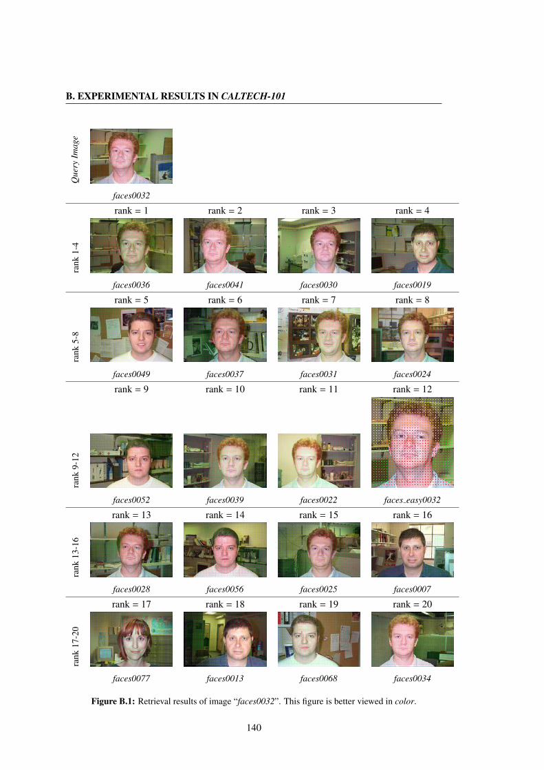
B. EXPERIMENTAL RESULTS IN CALTECH-101
Que
ryIm
age
faces0032
rank = 1 rank = 2 rank = 3 rank = 4
rank
1-4
faces0036 faces0041 faces0030 faces0019
rank = 5 rank = 6 rank = 7 rank = 8
rank
5-8
faces0049 faces0037 faces0031 faces0024
rank = 9 rank = 10 rank = 11 rank = 12
rank
9-12
faces0052 faces0039 faces0022 faces easy0032
rank = 13 rank = 14 rank = 15 rank = 16
rank
13-1
6
faces0028 faces0056 faces0025 faces0007
rank = 17 rank = 18 rank = 19 rank = 20
rank
17-2
0
faces0077 faces0013 faces0068 faces0034
Figure B.1: Retrieval results of image “faces0032”. This figure is better viewed in color.
140

Que
ryIm
age
faces0036
rank = 1 rank = 2 rank = 3 rank = 4
rank
1-4
faces0028 faces0037 faces0019 faces0030
rank = 5 rank = 6 rank = 7 rank = 8
rank
5-8
faces0024 faces0032 faces0039 faces0035
rank = 9 rank = 10 rank = 11 rank = 12
rank
9-12
faces0041 faces easy0027 faces easy0036 faces0013
rank = 13 rank = 14 rank = 15 rank = 16
rank
13-1
6
faces0060 faces0001 faces0052 faces0025
rank = 17 rank = 18 rank = 19 rank = 20
rank
17-2
0
faces0007 faces0005 faces0049 faces0038
Figure B.2: Retrieval results of image “faces0036”. This figure is better viewed in color.
141

B. EXPERIMENTAL RESULTS IN CALTECH-101
Que
ryIm
age
faces0038
rank = 1 rank = 2 rank = 3 rank = 4
rank
1-4
faces easy0038 faces0024 faces easy0039 faces0001
rank = 5 rank = 6 rank = 7 rank = 8
rank
5-8
faces0035 faces0036 faces0072 faces0037
rank = 9 rank = 10 rank = 11 rank = 12
rank
9-12
faces0028 faces0060 faces0019 faces0058
rank = 13 rank = 14 rank = 15 rank = 16
rank
13-1
6
faces0041 faces0031 faces0076 faces0039
rank = 17 rank = 18 rank = 19 rank = 20
rank
17-2
0
faces0073 faces0023 faces0029 faces0069
Figure B.3: Retrieval results of image “faces0038”. This figure is better viewed in color.
142

Que
ryIm
age
faces0039
rank = 1 rank = 2 rank = 3 rank = 4
rank
1-4
faces easy0039 faces0037 faces0036 faces0024
rank = 5 rank = 6 rank = 7 rank = 8
rank
5-8
faces0031 faces0041 faces0025 faces0035
rank = 9 rank = 10 rank = 11 rank = 12
rank
9-12
faces0001 faces0030 faces0032 faces0052
rank = 13 rank = 14 rank = 15 rank = 16
rank
13-1
6
faces0028 faces0022 faces0044 faces0040
rank = 17 rank = 18 rank = 19 rank = 20
rank
17-2
0
faces0012 faces0019 faces0006 faces0013
Figure B.4: Retrieval results of image “faces0039”. This figure is better viewed in color.
143

B. EXPERIMENTAL RESULTS IN CALTECH-101
Que
ryIm
age
faces0049
rank = 1 rank = 2 rank = 3 rank = 4
rank
1-4
faces easy0049 faces0052 faces0037 faces0068
rank = 5 rank = 6 rank = 7 rank = 8
rank
5-8
faces0058 faces0024 faces0048 faces0019
rank = 9 rank = 10 rank = 11 rank = 12
rank
9-12
faces0006 faces0034 faces0030 faces0031
rank = 13 rank = 14 rank = 15 rank = 16
rank
13-1
6
faces0005 faces0080 faces0032 faces0059
rank = 17 rank = 18 rank = 19 rank = 20
rank
17-2
0
faces0012 faces0007 faces0044 faces0013
Figure B.5: Retrieval results of image “faces0049”. This figure is better viewed in color.
144

(1) “accordion” (2) “beaver” (3) “car side”
(4) “cougar body” (5) “crocodile head” (6) “crocodile”
(7) “dalmatian” (8) “emu” (9) “faces”
(10) “ferry” (11) “flamingo head” (12) “gerenuk”Figure is continued on next page
145

B. EXPERIMENTAL RESULTS IN CALTECH-101
(13) “hawksbill” (14) “hedgehog” (15) “joshua tree”
(16) “mayfly” (17) “pagoda” (18) “sea horse”
(19) “trilobite” (20) “wrench”
Figure B.6: The distribution of average precision values for query images in 19 surpassing classes+ a category “car side” that only contains grayscale images, on the whole Caltech-101 dataset. Thecomparison is evaluated between SPM and BBoW (KKM) at level 1. Each image is partitioned into4 subgraphs.
146

Appendix C
Experimental Results in PPMI
BBoVW versus SPM in 12 binary category of PPMI
In PPMI dataset [158, 159], we have used two different distance metrics: L1 distance or L2
distance, as the measure to compute the cost matrix value (see Equation (4.10)) for (sub)graphs
matching via Hungarian algorithm.
In this Appendix, we are interested in the influence of these two metrics on image retrieval
in BBoW model. We also present the performance of SPM [4] as a side-by-side comparison.
The impact of L1 and L2 metrics on performance of image retrieval is investigated in Table C.1
and Table C.2.
147

C. EXPERIMENTAL RESULTS IN PPMI
Table C.1: The retrieval performance (mAP) on PPMI dataset, using L1 distance as cost matrixvalue for graph matching via Hungarian algorithm.
Category BBoWSingle Level
1
BBoWSingle Level
2
BBoWPyramidLevel 1
BBoWPyramidLevel 2
SPMPyramidLevel 2
bassoon 0.111035 0.113260 0.109303 0.110617 0.135067cello 0.119489 0.112404 0.115846 0.115524 0.126036
clarinet 0.116817 0.110903 0.117761 0.116395 0.114140
erhu 0.106178 0.102879 0.107562 0.106756 0.129702flute 0.107483 0.106279 0.109405 0.109117 0.110948
frenchhorn 0.106507 0.113634 0.107040 0.108762 0.129498guitar 0.132001 0.123785 0.139362 0.136860 0.143438harp 0.116316 0.121244 0.125459 0.125616 0.161372
recorder 0.124170 0.114372 0.126650 0.125308 0.116781
saxophone 0.103004 0.109306 0.099857 0.101788 0.108571
trumpet 0.114199 0.112452 0.114173 0.114380 0.109890
violin 0.104072 0.110334 0.102756 0.104535 0.105030
148

Table C.2: The retrieval performance (mAP) on PPMI dataset, using L2 distance as cost matrixvalue for graph matching Hungarian algorithm.
Category BBoWSingle Level
1
BBoWSingle Level
2
BBoWPyramidLevel 1
BBoWPyramidLevel 2
SPMPyramidLevel 2
bassoon 0.110804 0.111185 0.109103 0.110027 0.135067cello 0.119039 0.111707 0.115819 0.115575 0.126036
clarinet 0.114322 0.109811 0.116659 0.115271 0.114140
erhu 0.105380 0.102210 0.107372 0.106662 0.129702flute 0.107309 0.106516 0.109183 0.108834 0.110948
frenchhorn 0.106298 0.111488 0.107063 0.108518 0.129498guitar 0.128309 0.121247 0.137139 0.134486 0.143438harp 0.115931 0.122908 0.125046 0.125451 0.161372
recorder 0.121758 0.113676 0.125542 0.124338 0.116781
saxophone 0.102728 0.108641 0.099691 0.101784 0.108571
trumpet 0.111228 0.111266 0.112511 0.113247 0.109890
violin 0.103785 0.109715 0.102760 0.104304 0.105030
149

C. EXPERIMENTAL RESULTS IN PPMI
150

Appendix D
Proofs
Claim A:
Given two L1 normalized histograms G = g1, . . . , gB and H = h1, . . . , hB with B bins,
i.e.B∑
b=1
gb = 1,B∑
b=1
hb = 1 and ∀b ∈ [1, B], gb ≥ 0, hb ≥ 0, we have:
Histogram intersection Equation (4.2) in Chapter 4
K∩(G,H) =
B∑b=1
min(gb, hb) ,
is the equivalent of the Equation (4.3) in Chapter 4
K∩(G,H) =12
B∑b=1
(gb + hb − |gb − hb|) .
Proof :
Case 1: if gb ≥ hb, b ∈ [1, B], then
12
(gb + hb − |gb − hb|) =12
(gb + hb − gb + hb)
=12
(2hb)
= hb
= min (gb, hb) .
151

D. PROOFS
Case 2: if gb < hb, b ∈ [1, B], then
12
(gb + hb − |gb − hb|) =12
(gb + hb − hb + gb)
=12
(2gb)
= gb
= min (gb, hb) .
and the claim is proven.
Claim B:
Histogram Intersection is equivalent to the use of the sum of absolute differences or city-
block metric, i.e. L1 distance.
Proof :
Given two L1 normalized histograms G = g1, . . . , gB and H = h1, . . . , hB with B bins,
i.e.B∑
b=1
gb = 1,B∑
b=1
hb = 1 and ∀b ∈ [1, B], gb ≥ 0, hb ≥ 0, as proven in Claim A, the histogram
intersection between G and H:
K∩(G,H) =
B∑b=1
min(gb, hb)
=12
B∑b=1
(gb + hb − |gb − hb|) .
Hence, we have:
K∩(G,H) =12
B∑b=1
gb +
B∑b=1
hb −
B∑b=1
| gb − hb |
=
12
1 + 1 −B∑
b=1
| gb − hb |
= 1 −
12
B∑b=1
| gb − hb |
= 1 −12
DL1 (G,H) .
and the claim is proven.
152

Appendix E
Statistical Test
E.1 Paired samples t-interval
We trust that the samples we take are random. Instead of taking independent samples, we
choose pair of samples, and we try to make the pair of samples as homogeneous as possible.
In ideal case, test on samples themselves.
E.2 Matched Paired t-test
We have two observations on each query image. So here we have dependant samples, and
methods based on independent samples would not be appropriate here. We are going to use the
paired difference procedure to analyse this data. To do so we first take the differences within
each pair. We would end up with these nd differences, where nd is the number of query image
from the same category, for example, ‘faces’ class in Caltech-101. Then, these nd differences
represent as single sample so that we can use one sample t-test to analyse these differences.
We denote xd as the mean of the differences for sample, µd as the mean of the differences
for population, the standard deviation of those differences of the samples is S d; the standard
deviation of those differences for population is σd; degree of freedom d f = nd − 1. We denote
the Confidence Interval as CI.
Let us examine these differences (either in box plot or in histogram) to make sure they are
nearly normal distribution.
We compute the mean of the differences between our observed sample from two methods
(KKM vs SPM). We want to know if there is a significant difference between two methods on
153

E. STATISTICAL TEST
those query images.
We investigate that by carrying out a one sample t-test, and we also construct a confidence
interval at confidence coefficient 95%.
E.2.1 Data preparation
Conditions to satisfy:
1. Pair data assumption: The sample data being tested by two methods SPM and BBoW
are not independent. So we can not use two-sample t-test because they fail to sample
independence conditions. We have a good reason to pair the data, as each pair of average
precision values are related to the same query image. Hence, the data are paired by
subject.
2. Random conditions: The subject (images) were not chosen randomly (i.e. images from
intra-class), so we will have to assume these results are representative.
3. Nearly normal: The distribution (see histogram/box plots) of differences is uni-model
and symmetric.
E.3 Matched Paired t-test and interval
Question: What is the magnitude of the difference for image from ‘faces’ category in
performance of image retrieval between SPM and BBoW (via KKM) individuals?
Step 1: Hypothesis
H0: BBoW (KKM) does not improve the performance of image retrieval µd = 0
H1 BBoW (KKM) does improve the performance of image retrieval µd > 0 (right tailed
t-test)
Step 2: Compute test statistic
S d =
√√∑xd
2 −(∑
xd)2
nd
nd − 1
=
√∑xd
2 − nd(xd)2
nd − 1. (E.1)
154
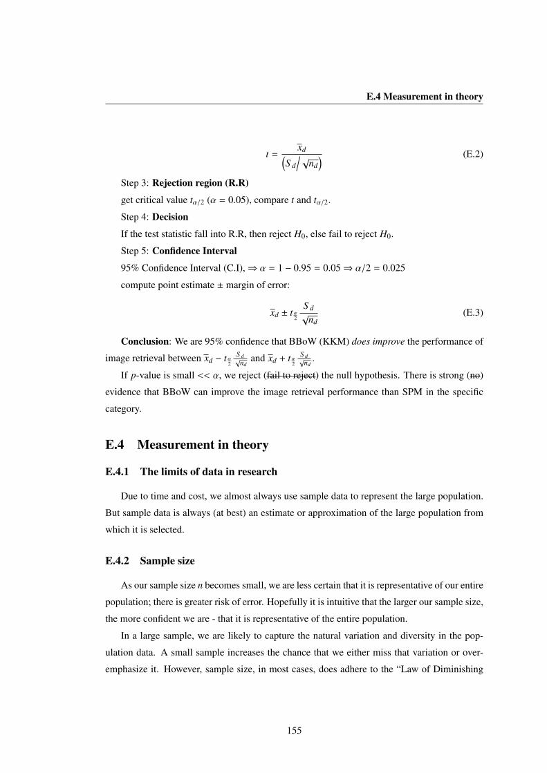
E.4 Measurement in theory
t =xd(
S d/√
nd) (E.2)
Step 3: Rejection region (R.R)
get critical value tα/2 (α = 0.05), compare t and tα/2.
Step 4: Decision
If the test statistic fall into R.R, then reject H0, else fail to reject H0.
Step 5: Confidence Interval
95% Confidence Interval (C.I),⇒ α = 1 − 0.95 = 0.05⇒ α/2 = 0.025
compute point estimate ± margin of error:
xd ± t α2
S d√
nd(E.3)
Conclusion: We are 95% confidence that BBoW (KKM) does improve the performance of
image retrieval between xd − t α2
S d√nd
and xd + t α2
S d√nd
.
If p-value is small << α, we reject (fail to reject) the null hypothesis. There is strong (no)
evidence that BBoW can improve the image retrieval performance than SPM in the specific
category.
E.4 Measurement in theory
E.4.1 The limits of data in research
Due to time and cost, we almost always use sample data to represent the large population.
But sample data is always (at best) an estimate or approximation of the large population from
which it is selected.
E.4.2 Sample size
As our sample size n becomes small, we are less certain that it is representative of our entire
population; there is greater risk of error. Hopefully it is intuitive that the larger our sample size,
the more confident we are - that it is representative of the entire population.
In a large sample, we are likely to capture the natural variation and diversity in the pop-
ulation data. A small sample increases the chance that we either miss that variation or over-
emphasize it. However, sample size, in most cases, does adhere to the “Law of Diminishing
155
E. STATISTICAL TEST
Returns”. There is a point when increasing the sample size offers no more statistical benefits,
which is good because it makes research more “doable”.
E.4.3 Data preparation
Is My Data Normal? Why? Many statistical techniques assume the data fits a normal distri-
bution. How could we tell if the data fits this shape: The normal standard curve. Does our data
have “goodness of fit” relative to the normal distribution? Tools to visualize data:
1. Histograms: the frequency of values over certain intervals is called “bins”; bar width.
Histogram can be misleading. The look of a histogram is largely dependent on the “bins”
size; the space between the tick marks.
2. Box Plots (Box and Whisker Plots) : Box plots display variation in samples of a statisti-
cal population without making any assumptions of the underlying statistical distribution:
box plots are non-parametric. The spacings between the different parts of the box indi-
cate the degree of dispersion (spread) and skewness in the data, and show outliers.
3. Stem and Leaf Plots
4. P-P Plots
5. Q-Q Plots
Degrees of freedom Degrees of freedom is one of the most difficult things to explain in
statistics. My explanation: Degrees of freedom is an adjustment to the sample size (n − 1) or
in other areas of state (n − 2) or more. It is linked to the idea that we are estimating something
about a larger population; often a population with variance/standard deviation is unknown.
Since we do not know the population variance and standard deviation, we have to use our
sample variance and standard deviation. So the degrees of freedom is a way of adjusting that
estimations. What it does, in practice, is that it gives a slightly larger margin of error or “wiggle
room” in our estimates. Other than that, just roll with it; it is a statistical adjustment.
156

E.4 Measurement in theory
E.4.4 The t distribution
When our sample size is n 6 30 and/or we do not know the variance/standard deviation of
the population, we use the t-distribution instead of the z-distribution (standard normal distribu-
tion).
The t-distribution allows us to use small samples; n 6 30. But to do so we sacrifice some
certainty in our calculations; margin-of-error trade-off. It is dynamic, it takes sample size into
account using n − 1 degree of freedom; there is a different t-distribution for any given sample
size. The bell curve shape is down (“squished”) in the middle and “fatter” on the end (tails);
squishier and fatter the sample size.
However, as n > 30 and definitely by n > 100, the t-distribution and standard normal z-
distribution become indistinguishable. They converge. i.e., when the sample size goes above
30, the t distribution and z distribution converges. Hence, t-distribution is more useful as sample
size is below 30.
Conditions for using t-test
1. The population standard deviation is unknown
2. The sample size is less than 30
Sample size does not matter for t-Test. If the sample is less than 30, we should always
do t-test and not Z-Scores. However the reverse is not true. You can still do t-Test even if
the sample size is greater than 30. Main reason to do t-tests are when you do not know the
population statistics like mean, standard deviation (SD) and they have to be estimated form the
sample. Whereas in z-Scores, you need to know the population mean and SD.
E.4.5 p-value method
Traditional methods use something called critical values, z score, p-value method does not
use them at all.
E.4.5.1 Basic of Hypothesis Testing
Null Hypothesis H0:
157
E. STATISTICAL TEST
P = #
µ = #
σ = #
Alter. Hypothesis H1:
P < #
µ > #
σ , #
left-tailed: H1 :<
right-tailed: H1 :>
two-tailed: H1 ,>
The p-value is a measure of the strength of the evidence against the null hypothesis. The
p-value is the probability of getting the observed value of the test statistic, or a value with even
greater evidence against H0, if the null hypothesis is actually true. The smaller the p-value, the
greater the evidence against the null hypothesis.
E.4.5.2 Level of significance
Conventionally, α = 0.01, α = 0.05, α = 0.10.
1. If we have a given significance level α, then reject H0 if p-value 6 α (cut-off for signifi-
cance).
2. If we do not have a given significance level, then it is not as cut-and-dried. Check the
distribution of p-value if H0 is true.
E.4.5.3 A very rough guideline
1. p-value < 0.01, very strong evidence against H0.
2. 0.01 < p-value < 0.05, strong evidence against H0.
3. 0.05 < p-value < 0.10, some weak evidence against H0.
4. p-value > 0.10, little or no evidence against H0.
158

E.4 Measurement in theory
E.4.5.4 Summary
1. If the P-value is low, the null must go (reject H0).
2. If the P-value is high, the null must fly (fail to reject H0, keep H0).
159

E. STATISTICAL TEST
160

References
[1] Otavio Augusto Bizetto Penatti, Eduardo Valle, and Ricardo da Silva Torres. Comparativestudy of global color and texture descriptors for web image retrieval. Journal of VisualCommunication and Image Representation, 23(2):359–380, 2012. iii, 7
[2] David G. Lowe. Distinctive image features from scale-invariant keypoints. In In InternationalJournal of Computer Vision, pages 91–110, 2004. iii, 6, 8, 19, 20, 31, 72, 73, 94, 95
[3] Ritendra Datta, Dhiraj Joshi, Jia Li, and James Ze Wang. Image retrieval: Ideas, influences,and trends of the new age. ACM Computing Surveys, 40(2), April 2008. iii, 1, 17, 18
[4] Svetlana Lazebnik, Cordelia Schmid, and Jean Ponce. Beyond bags of features: Spatial pyra-mid matching for recognizing natural scene categories. In Computer Vision and PatternRecognition, 2006 IEEE Computer Society Conference on, 2, pages 2169–2178, 2006. iv, 2,3, 22, 32, 83, 85, 87, 88, 95, 107, 113, 147
[5] Jianbo Shi and Jitendra Malik. Normalized Cuts and image segmentation. IEEE Transactionson Pattern Analysis and Machine Intelligence, 22(8):888–905, 2000. iv, 23, 34, 47, 48, 49, 51
[6] Greg Mori, Xiaofeng Ren, Alexei A. Efros, and Jitendra Malik. Recovering human body con-figurations: combining segmentation and recognition. In IEEE Computer Society Conferenceon Computer Vision and Pattern Recognition, 2, pages 326–333, 2004. iv, 23
[7] Svebor Karaman. Indexation de la video portee : application a l`etude epidemiologique desmaladies liees a l`age. PhD thesis, Universite Bordeaux 1, 2011. iv, 27, 28
[8] Yuri Boykov and Vladimir Kolmogorov. An experimental comparison of min-Cut/max-Flowalgorithms for energy minimization in vision. IEEE Transactions on Pattern Analysis andMachine Intelligence, 26(9):1124–1137, 2004. v, 39, 40, 42, 47, 74, 94
[9] Yuri Boykov, Olga Veksler, and Ramin Zabih. Fast approximate energy minimization viaGraph Cuts. IEEE Transactions on Pattern Analysis and Machine Intelligence, 23(11):1222–1239, 2001. v, 39, 42, 43, 47, 94
[10] Rouhollah Rahmani, Sally A. Goldman, Hui Zhang, John Krettek, and Jason E. Fritts. Lo-calized content based image retrieval. In Multimedia Information Retrieval, pages 227–236.ACM, 2005. v, ix, 46, 91, 124
161

REFERENCES
[11] Inderjit S. Dhillon, Yuqiang Guan, and Brian Kulis. A fast kernel-based multilevel algorithmfor graph clustering. In International Conference on Knowledge Discovery and Data Mining,pages 629–634. ACM, 2005. v, 55, 56
[12] George Karypis and Vipin Kumar. Multilevel k-way partitioning scheme for irregular graphs.Journal of Parallel and Distributed Computing, 48(1):96129, 1998. v, 56, 74
[13] Bastian Leibe, Ales Leonardis, and Bernt Schiele. Combined object categorization and seg-mentation with an implicit shape model. In In ECCV workshop on statistical learning incomputer vision, 2004. xviii, 2, 24
[14] Arnold W. M. Smeulders, Marcel Worring, Simone Santini, Amarnath Gupta, and Ramesh
Jain. Content-based image retrieval at the end of the early years. IEEE Transactions onPattern Analysis and Machine Intelligence, 22(12):1349–1380, 2000. 1, 17
[15] Ritendra Datta, Jia Li, and James Ze Wang. Content-based image retrieval: approaches andtrends of the new age. In Multimedia Information Retrieval, pages 253–262, 2005. 1, 17
[16] J. Sivic and A. Zisserman. Video Google: a text retrieval approach to object matching invideos. In International Conference on Computer Vision, 2, pages 1470–1477, October 2003. 1,19, 71, 83
[17] Xiaofeng Ren and Jitendra Malik. Learning a classification model for segmentation. InInternational Conference on Computer Vision, 1, pages 10–17, 2003. 1, 23, 51
[18] Stan Birchfield and Sriram Rangarajan. Spatiograms versus Histograms for region-basedtracking. In IEEE Computer Society Conference on Computer Vision and Pattern Recognition,pages 1158–1163, 2005. 2, 24
[19] Ankur Agarwal and Bill Triggs. Hyperfeatures - Multilevel local coding for visual recogni-tion. In European Conference on Computer Vision, pages 30–43, 2006. 2, 121
[20] Josip Krapac, Jakob J. Verbeek, and Frederic Jurie. Modeling spatial layout with fisher vectorsfor image categorization. In International Conference on Computer Vision, pages 1487–1494,2011. 2, 25, 120
[21] Jorge Sanchez, Florent Perronnin, and Teofilo Emıdio de Campos. Modeling the spatial layoutof images beyond spatial pyramids. Pattern Recognition Letters, 33(16):2216–2223, 2012. 2,25, 120
[22] O. Duchenne, A. Joulin, and J. Ponce. A graph-matching kernel for object categorization. InInternational Conference on Computer Vision, pages 1792–1799, 2011. 2, 27
[23] Jaume Gibert, Ernest Valveny, and Horst Bunke. Graph embedding in vector spaces by nodeattribute statistics. Pattern Recognition, 45(9):3072–3083, 2012. 2
162

REFERENCES
[24] Horst Bunke and Kaspar Riesen. Towards the unification of structural and statistical patternrecognition. Pattern Recognition Letters, 33(7):811–825, 2012. 2, 27
[25] Ricardo da Silva Torres and Alexandre X. Falcao. Content-Based Image Retrieval: Theoryand Applications. Revista de Informatica Teorica e Aplicada, 13(2):161–185, 2006. 6, 17
[26] Krystian Mikolajczyk and Cordelia Schmid. Scale & affine invariant interest point detectors.International Journal of Computer Vision, 60(1):63–86, 2004. 7
[27] Djemel Ziou and Salvatore Tabbone. Edge detection techniques - An overview. InternationalJournal of Pattern Recognition and Image Analysis, 8:537–559, 1998. 7
[28] Chris Harris and Mike Stephens. A combined corner and edge detector. In Alvey VisionConference, pages 1–6, 1988. 7, 24
[29] Tony Lindeberg. Feature detection with automatic scale selection. International Journal ofComputer Vision, 30(2):79–116, 1998. 7
[30] Krystian Mikolajczyk, Tinne Tuytelaars, Cordelia Schmid, Andrew Zisserman, Jiri Matas,Frederik Schaffalitzky, Timor Kadir, and Luc J. Van Gool. A comparison of affine regiondetectors. International Journal of Computer Vision, 65(1-2):43–72, 2005. 7
[31] David G. Lowe. Object recognition from local scale-invariant features. In International Con-ference on Computer Vision, pages 1150–1157, 1999. 8, 20, 71
[32] Yan Ke and Rahul Sukthankar. PCA-SIFT: A more distinctive representation for local imagedescriptors. In IEEE Computer Society Conference on Computer Vision and Pattern Recogni-tion, pages 506–513, 2004. 9
[33] R. Arandjelovic and A. Zisserman. Three things everyone should know to improve objectretrieval. In IEEE Conference on Computer Vision and Pattern Recognition, 2012. 9, 78, 98
[34] John M. Winn, Antonio Criminisi, and Thomas P. Minka. Object categorization by learneduniversal visual dictionary. In International Conference on Computer Vision, pages 1800–1807, 2005. 9
[35] Herbert Bay, Tinne Tuytelaars, and Luc J. Van Gool. SURF: Speeded Up Robust Features.In European Conference on Computer Vision, pages 404–417, 2006. 9, 20, 27, 31, 72, 94, 95
[36] Tinne Tuytelaars. Dense interest points. In IEEE Computer Society Conference on ComputerVision and Pattern Recognition, pages 2281–2288, 2010. 10, 31
[37] Jian Wu, Zhiming Cui, Victor S. Sheng, Pengpeng Zhao, Dongliang Su, and Shengrong Gong.A comparative study of SIFT and its variants. Measurement Science Review, 13(3):122–131,2013. 10, 94
163
REFERENCES
[38] Charles T. Zahn and Ralph Z. Roskies. Fourier descriptors for plane closed curves. IEEETransactions on Computers, 21(3):269–281, March 1972. 10
[39] Farzin Mokhtarian and Riku Suomela. Robust image corner detection through curvaturescale space. IEEE Transactions on Pattern Analysis and Machine Intelligence, 20(12):1376–1381, 1998. 10
[40] A. Khotanzad and Y. H. Hong. Invariant image recognition by Zernike moments. IEEETransactions on Pattern Analysis and Machine Intelligence, 12(5):489–497, May 1990. 10
[41] Julien Ricard, David Coeurjolly, and Atilla Baskurt. Generalizations of angular radial trans-form for 2D and 3D shape retrieval. Pattern Recognition Letters, 26(14):2174–2186, 2005. 10
[42] A. Amanatiadis, V.G. Kaburlasos, A. Gasteratos, and S.E. Papadakis. Evaluation of shapedescriptors for shape-based image retrieval. Image Processing, IET, 5(5):493–499, August2011. 10
[43] Dean S. Messing, Peter van Beek, and James H. Errico. The MPEG-7 colour structure de-scriptor: image description using colour and local spatial information. In InternationalConference on Image Processing, 1, pages 670–673, 2001. 11
[44] Michael J. Swain and Dana H. Ballard. Color indexing. International Journal of ComputerVision, 7(1):11–32, 1991. 11, 77, 82, 87
[45] Markus A. Stricker and Markus Orengo. Similarity of color images. In Storage and Retrievalfor Image and Video Databases (SPIE), pages 381–392, 1995. 11, 25
[46] Greg Pass, Ramin Zabih, and Justin Miller. Comparing images using color coherence vectors.In ACM International Conference on Multimedia, pages 65–73, 1996. 12
[47] Jing Huang, Ravi Kumar, Mandar Mitra, Wei-Jing Zhu, and Ramin Zabih. Image indexingusing color correlograms. In IEEE Computer Society Conference on Computer Vision andPattern Recognition, pages 762–768, 1997. 12
[48] Timo Ojala, Matti Pietikainen, and Topi Maenpaa. Multiresolution gray-scale and rotationinvariant texture classification with local binary patterns. IEEE Transactions on PatternAnalysis and Machine Intelligence, 24(7):971–987, 2002. 13, 121
[49] Robert M. Haralick, K. Sam Shanmugam, and Its’hak Dinstein. Textural features for imageclassification. IEEE Transactions on Systems, Man, and Cybernetics, 3(6):610–621, 1973. 13,15, 25
[50] Julian Besag. Spatial interaction and the statistical analysis of lattice systems. Journal of theRoyal Statistical Society. Series B, 36(2):192–236, 1974. 13, 38
164

REFERENCES
[51] Stuart Geman and Donald Geman. Stochastic relaxation, gibbs distributions, and theBayesian restoration of images. IEEE Transactions on Pattern Analysis and Machine Intel-ligence, 6:721–741, 1984. 13, 38
[52] Jianchang Mao and Anil K. Jain. Texture classification and segmentation using multiresolu-tion simultaneous autoregressive models. Pattern Recognition, 25(2):173–188, 1992. 13
[53] R. Sriram, Joseph M. Francos, and William A. Pearlman. Texture coding using a wold de-composition model. IEEE Transactions on Image Processing, pages 1382–1386, 1996. 13
[54] S.J.Park, D.K.Park, and C. S. Won. Core experiments on MPEG-7 edge histogram descrip-tor. In MPEG document, M5984, Geneva, May 2000. 13
[55] Dong Kwon Park, Yoon Seok Jeon, and Chee Sun Won. Efficient use of local edge histogramdescriptor. In Proceedings of the ACM Multimedia Workshops, pages 51–54. ACM Press, 2000.13
[56] John R. Smith and Shih-Fu Chang. Transform features for texture classification and discrim-ination in large image databases. In International Conference on Image Processing, pages407–411. IEEE, 1994. 13
[57] Gert Van de Wouwer, Paul Scheunders, and Dirk Van Dyck. Statistical texture characteri-zation from discrete wavelet representations. IEEE Transactions on Image Processing, pages592–598, 1999. 13
[58] Changren Zhu and Runsheng Wang. Local multiple patterns based multiresolution gray-scaleand rotation invariant texture classification. Information Sciences, 187:93–108, 2012. 14
[59] Andre Ricardo Backes, Dalcimar Casanova, and Odemir Martinez Bruno. Texture analysisand classification: A complex network-based approach. Information Sciences, 219:168–180,2013. 14
[60] Matti Pietikainen, Abdenour Hadid, Guoying Zhao, and Timo Ahonen. Computer vision usinglocal binary patterns. Springer, 2011. 14
[61] Hee-Jung Bae and Sung-Hwan Jung. Image retrieval using texture based on DCT. In Inter-national Conference on Information, Communications and Signal Processing, pages 1065–1068,Sepember 1997. 15
[62] Isaac Ng, Tele Tan, and Josef Kittler. On local linear transform and Gabor filter represen-tation of texture. In IAPR International Conference on Pattern Recognition, Image, Speech andSignal Analysis, pages 627–631, August 1992. 15
[63] Aude Oliva and Antonio Torralba. Modeling the shape of the scene: A holistic representationof the spatial envelope. International Journal of Computer Vision, 42(3):145–175, 2001. 15, 16
165
REFERENCES
[64] Aude Oliva. Gist of the scene. In Neurobiology of Attention, page 251256, 2005. 15
[65] Aude Oliva and Antonio Torralba. Building the gist of a scene: the role of global imagefeatures in recognition. In Progress in Brain Research, page 2336, 2006. 16
[66] Antonio Torralba and Aude Oliva. Depth estimation from image structure. IEEE Transac-tions on Pattern Analysis and Machine Intelligence, 24(9):1226–1238, 2002. 16
[67] James Hays and Alexei A. Efros. Scene completion using millions of photographs. ACMTransactions on Graphics, 26(3):4, 2007. 16
[68] Antonio Torralba, Kevin P. Murphy, William T. Freeman, and Mark A. Rubin. Context-basedvision system for place and object recognition. In International Conference on ComputerVision, pages 273–280, 2003. 16
[69] Antonio Torralba. Contextual priming for object detection. International Journal of Com-puter Vision, 53(2):169–191, 2003.
[70] Antonio Torralba, Robert Fergus, and William T. Freeman. 80 million tiny images: A largedata set for nonparametric object and scene recognition. IEEE Transactions on Pattern Anal-ysis and Machine Intelligence, 30(11):1958–1970, 2008. 16
[71] Matthijs Douze, Herve Jegou, Harsimrat Sandhawalia, Laurent Amsaleg, and Cordelia
Schmid. Evaluation of GIST descriptors for web-scale image search. In ACM InternationalConference on Image and Video Retrieval, 2009. 16
[72] A. Bhattacharyya. On a measure of divergence between two statistical populations definedby their probability distributions. Bulletin of the Calcutta Mathematical Society, 35:99109,1943. 17
[73] Frank J. Aherne, Neil A. Thacker, and Peter I Rockett. The Bhattacharyya metric as anabsolute similarity measure for frequency coded data. Kybernetika, 34(4):363368, 1998. 17
[74] Amarnath Gupta and Ramesh Jain. Visual information retrieval. Communications of the ACM,40(5):70–79, 1997. 17
[75] Alberto Del Bimbo. Visual information retrieval. Morgan Kaufmann Publishers, San Francisco,CA, USA, 1999. 34
[76] Abby Goodrum. Image information retrieval: An overview of current research. InformingScience, 3:2000, 2000. 17
[77] F.Idris and S.Panchanathan. Review of image and video indexing techniques. Journal of VisualCommunication and Image Representation, 8(2):146166, 1997. 18
[78] Vittorio Ferrari, Frederic Jurie, and Cordelia Schmid. From images to shape models forobject detection. International Journal of Computer Vision, 87(3):284–303, 2010. 18
166

REFERENCES
[79] Diane Larlus, Jakob J. Verbeek, and Frederic Jurie. Category level object segmentation bycombining Bag-of-Words models with Dirichlet processes and random fields. InternationalJournal of Computer Vision, 88(2):238–253, 2010. 18
[80] Gabriella Csurka, Christopher R. Dance, Lixin Fan, Jutta Willamowski, and Cedric Bray. Vi-sual categorization with bags of keypoints. In In Workshop on Statistical Learning in ComputerVision, ECCV, pages 1–22, 2004. 19, 21, 71
[81] B. Julesz. Textons, the elements of texture perception, and their interactions. Nature,290(5802):9197, March 1981. 19
[82] Thomas K. Leung and Jitendra Malik. Representing and recognizing the visual appear-ance of materials using three-dimensional textons. International Journal of Computer Vision,43(1):29–44, 2001. 19
[83] Gerard Salton and Michael J. McGill. Introduction to modern information retrieval. McGraw-Hill computer science series. McGraw-Hill, 1983. 19
[84] J. B. MacQueen. Some methods for classification and analysis of multiVariate observations.In Proceedings of 5-th Berkeley Symposium on Mathematical Statistics and Probability, 1, pages281–297. Berkeley, University of California Press, 1967. 20, 52
[85] Jan van Gemert, Cor J. Veenman, Arnold W. M. Smeulders, and Jan-Mark Geusebroek. Visualword ambiguity. IEEE Transactions on Pattern Analysis and Machine Intelligence, 32(7):1271–1283, 2010. 20, 94
[86] Piotr Koniusz and Krystian Mikolajczyk. Soft assignment of visual words as linear coor-dinate coding and optimisation of its reconstruction error. In International Conference onImage Processing, pages 2413–2416, 2011.
[87] Vinay Garg, Sreekanth Vempati, and C.V. Jawahar. Bag of visual words: A soft clusteringbased exposition. In National Conference on Computer Vision, Pattern Recognition, ImageProcessing and Graphics, pages 37–40, December 2011.
[88] Yubin Kuang, Kalle Åstrom, Lars Kopp, Magnus Oskarsson, and Martin Byrod. Optimizingvisual vocabularies using soft assignment entropies. In Asian Conference on Computer Vision,pages 255–268, 2010. 20, 94
[89] Alex Levinshtein, Adrian Stere, Kiriakos N. Kutulakos, David J. Fleet, Sven J. Dickinson, and
Kaleem Siddiqi. TurboPixels: Fast superpixels using geometric flows. IEEE Transactions onPattern Analysis and Machine Intelligence, 31(12):2290–2297, 2009. 23
[90] R. Achanta, A. Shaji, K. Smith, A. Lucchi, P. Fua, and S. Susstrunk. SLIC superpixels com-pared to state-of-the-art superpixel methods. IEEE Transactions on Pattern Analysis andMachine Intelligence, 34(11):2274–2282, November 2012. 23
167

REFERENCES
[91] Michael Van den Bergh, Xavier Boix, Gemma Roig, Benjamin de Capitani, and Luc J. Van Gool.SEEDS: Superpixels extracted via energy-driven sampling. In European Conference on Com-puter Vision, pages 13–26, 2012. 23
[92] Alexander Schick, Mika Fischer, and Rainer Stiefelhagen. Measuring and evaluating thecompactness of superpixels. In International Conference on Pattern Recognition, pages 930–934, 2012. 23
[93] Ciaran O Conaire, Noel E. O’Connor, and Alan F. Smeaton. An improved spatiogram similar-ity measure for robust object localisation. In International Conference on Acoustics, Speech,and Signal Processing, pages 1069–1072, 2007. 24
[94] Dorin Comaniciu, Visvanathan Ramesh, and Peter Meer. Real-time tracking of non-rigidobjects using Mean Shift. In IEEE Computer Society Conference on Computer Vision andPattern Recognition, 2000. 24
[95] Rahat Khan, Cecile Barat, Damien Muselet, and Christophe Ducottet. Spatial orientations ofvisual word pairs to improve Bag-of-Visual-Words model. In British Machine Vision Confer-ence, pages 1–11, 2012. 25
[96] Florent Perronnin and Christopher R. Dance. Fisher kernels on visual vocabularies for im-age categorization. In IEEE Computer Society Conference on Computer Vision and PatternRecognition, 2007. 25
[97] Florent Perronnin, Jorge Sanchez, and Thomas Mensink. Improving the fisher kernel forlarge-scale image classification. In European Conference on Computer Vision, pages 143–156,2010.
[98] Florent Perronnin, Yan Liu, Jorge Sanchez, and Herve Poirier. Large-scale image retrievalwith compressed Fisher vectors. In IEEE Computer Society Conference on Computer Visionand Pattern Recognition, pages 3384–3391, 2010.
[99] K. Simonyan, O. Parkhi, A. Vedaldi, and A. Zisserman. Fisher vector faces in the wild. InBritish Machine Vision Conference, 2013. 25, 120
[100] Jianchao Yang, Kai Yu, Yihong Gong, and T. Huang. Linear spatial pyramid matching usingsparse coding for image classification. In IEEE Computer Society Conference on ComputerVision and Pattern Recognition, pages 1794–1801, June 2009. 25
[101] Jinjun Wang, Jianchao Yang, Kai Yu, Fengjun Lv, Thomas S. Huang, and Yihong Gong. Locality-constrained linear coding for image classification. In IEEE Computer Society Conference onComputer Vision and Pattern Recognition, pages 3360–3367, 2010. 25
[102] Sancho McCann and David G. Lowe. Spatially local coding for object recognition. In AsianConference on Computer Vision, pages 204–217, 2012. 25, 120
168
REFERENCES
[103] Wei Huang, Yan Gao, and Kap Luk Chan. A review of region-based image retrieval. Journalof Signal Processing Systems, 59(2):143161, 2010. 25
[104] Narendra Ahuja and Sinisa Todorovic. From region based image representation to objectdiscovery and recognition. In Structural, Syntactic, and Statistical Pattern Recognition, JointIAPR International Workshop, 6218 of Lecture Notes in Computer Science, pages 1–19. Springer,2010. 25
[105] Feng Jing, Mingjing Li, HongJiang Zhang, and Bo Zhang. An effective region-based imageretrieval framework. In ACM International Conference on Multimedia, pages 456–465, 2002.26
[106] Feng Jing, Mingjing Li, Lei Zhang, HongJiang Zhang, and Bo Zhang. Learning in region-basedimage retrieval. In ACM International Conference on Image and Video Retrieval, pages 206–215, 2003.
[107] Feng Jing, Mingjing Li, HongJiang Zhang, and Bo Zhang. An efficient and effective region-based image retrieval framework. IEEE Transactions on Image Processing, 13(5):699–709,2004. 26
[108] Jean-Francois Omhover and Marcin Detyniecki. STRICT: An image retrieval platform forqueries based on regional content. In ACM International Conference on Image and VideoRetrieval, pages 473–482, 2004. 26
[109] Jean-Francois Omhover and Marcin Detyniecki. Fast gradual matching measure for imageretrieval based on visual similarity and spatial relations. International Journal of IntelligentSystems, 21(7):711–723, 2006. 26
[110] Philippe Henri Gosselin, Matthieu Cord, and Sylvie Philipp-Foliguet. Kernels on bags of fuzzyregions for fast object retrieval. In ICIP, pages 177–180, 2007. 26
[111] Remi Vieux, Jenny Benois-Pineau, and Jean-Philippe Domenger. Content based image retrievalusing Bag-Of-Regions. In International Conference on Advances in Multimedia Modeling,pages 507–517, 2012. 26, 78
[112] Justine Lebrun, Sylvie Philipp-Foliguet, and Philippe Henri Gosselin. Image retrieval withgraph kernel on regions. In International Conference on Pattern Recognition, pages 1–4, 2008.27
[113] Justine Lebrun, Philippe Henri Gosselin, and Sylvie Philipp-Foliguet. Inexact graph match-ing based on kernels for object retrieval in image databases. Image and Vision Computing,29(11):716–729, 2011. 27
[114] Hichem Sahbi, Jean-Yves Audibert, Jaonary Rabarisoa, and Renaud Keriven. Object recogni-tion and retrieval by context dependent similarity kernels. In CBMI, pages 216–223, 2008.27
169

REFERENCES
[115] Edwin R. Hancock, Andrea Torsello, Francisco Escolano, and Luc Brun. Special issue ongraph-based representations in computer vision. Computer Vision and Image Understanding,115(7):903–904, 2011. 29
[116] Jonathan Richard Shewchuk. Triangle: Engineering a 2D quality mesh generator and de-launay triangulator. In Workshop on Applied Computational Geometry, pages 203–222, 1996.33
[117] Y. Boykov, O. Veksler, and R. Zabih. Markov random fields with efficient approximations.In Computer Vision and Pattern Recognition, 1998. Proceedings. 1998 IEEE Computer SocietyConference on, pages 648–655, June 1998. 34
[118] Charless Fowlkes, Serge Belongie, Fan R. K. Chung, and Jitendra Malik. Spectral groupingusing the nystrom method. IEEE Transactions on Pattern Analysis and Machine Intelligence,26(2):214–225, 2004. 51
[119] Inderjit S. Dhillon, Yuqiang Guan, and Brian Kulis. Weighted graph cuts without eigenvec-tors a multilevel approach. IEEE Transactions on Pattern Analysis and Machine Intelligence,29(11):1944–1957, November 2007. 34, 51, 52
[120] Shengjiu Wang. A robust CBIR approach using local color histograms. Technical report,University of Alberta, 2001. 34
[121] Pratheep Anantharatnasamy, Kaavya Sriskandaraja, Vahissan Nandakumar, and Sampath Dee-galla. Fusion of colour, shape and texture features for content based image retrieval. InInternational Conference on Computer Science Education, pages 422–427, April 2013. 34
[122] Carsten Rother, Vladimir Kolmogorov, and Andrew Blake. GrabCut - Interactive fore-ground extraction using iterated Graph Cuts. ACM Transactions on Graphics (SIGGRAPH),August 2004. 35, 47
[123] Inderjit S. Dhillon, Yuqiang Guan, and Brian Kulis. Kernel k-means: spectral clusteringand Normalized Cuts. In Proceedings of the Tenth ACM SIGKDD International Conference onKnowledge Discovery and Data Mining, pages 551–556, 2004. 37, 50, 51, 54, 58
[124] Pedro F. Felzenszwalb and Daniel P. Huttenlocher. Efficient graph-based image segmenta-tion. International Journal of Computer Vision, 59(2):167–181, 2004. 38, 74
[125] Yuri Boykov and Marie-Pierre Jolly. Interactive graph cuts for optimal boundary & regionsegmentation of objects in N-D images. In International Conference on Computer Vision, pages105–112, 2001. 39, 47
[126] Vladimir Kolmogorov and Ramin Zabih. What energy functions can be minimized via graphcuts. IEEE Transactions on Pattern Analysis and Machine Intelligence, 26:65–81, 2004. 39, 94
170
REFERENCES
[127] L. R. Ford and D. R. Fulkerson. Maximal flow through a network. Canadian Journal ofMathematics, 8:399404, 1956. 39
[128] L. R. Ford Jr. and D. R. Fulkerson. Flows in networks. Princeton University Press, 1962. 40
[129] Zhenyu Wu and Richard M. Leahy. An optimal graph theoretic approach to data clustering:Theory and its application to image segmentation. IEEE Transactions on Pattern Analysis andMachine Intelligence, 15(11):1101–1113, 1993. 47
[130] Nikos Komodakis and Georgios Tziritas. Approximate labeling via Graph Cuts basedon linear programming. IEEE Transactions on Pattern Analysis and Machine Intelligence,29(8):1436–1453, 2007. 47
[131] Andrew Delong, Anton Osokin, Hossam N. Isack, and Yuri Boykov. Fast approximate energyminimization with label costs. International Journal of Computer Vision, 96(1):1–27, 2012. 47
[132] Dong Yan and Ma Yongzhuang. Image restoration using Graph Cuts with adaptive smooth-ing. In International Conference on Information Acquisition, pages 152–156, July 2007. 47
[133] Tommy W. H. Tang and Albert C. S. Chung. Non-rigid image registration using Graph-cuts.In International Conference on Medical Image Computing and Computer-Assisted Intervention,pages 916–924, 2007. 47
[134] Ronald W. K. So, Tommy W. H. Tang, and Albert C. S. Chung. Non-rigid image registrationof brain magnetic resonance images using graph-cuts. Pattern Recognition, 44(10-11):2450–2467, 2011. 47
[135] Nicolas Papadakis and Aurelie Bugeau. Tracking with occlusions via Graph Cuts. IEEETransactions on Pattern Analysis and Machine Intelligence, 33(1):144–157, 2011. 47
[136] Gene H. Golub and Charles F. Van Loan. Matrix computations. Johns Hopkins Press, 2ndedition, 1989. 49
[137] Alex Pothen, Horst D. Simon, and Kan-Pu Liou. Partitioning sparse matrices with eigenvec-tors of graphs. SIAM Journal on Matrix Analysis and Applications, 11(3):430–452, May 1990.49
[138] B. W. Kernighan and S. Lin. An efficient heuristic procedure for partitioning graphs. TheBell system technical journal, 49(1):291–307, 1970. 51
[139] Pak K. Chan, Martine D. F. Schlag, and Jason Y. Zien. Spectral k-way ratio-cut partition-ing and clustering. IEEE Transactions on Computer-Aided Design of Integrated Circuits andSystems, 13(9):1088–1096, 1994. 51, 52
[140] Stella X.Yu and Jianbo Shi. Multiclass spectral clustering. In International Conference onComputer Vision, 1, pages 313–319, 2003. 51
171

REFERENCES
[141] Inderjit Dhillon, Yuqiang Guan, and Brian Kulis. A unified view of kernel k-means, spectralclustering and graph partitioning. Technical Report TR-04-25, University of Texas Dept. ofComputer Science, 2005. 52, 57
[142] Bernhard Scholkopf, Alex J. Smola, and Klaus-Robert Muller. Nonlinear component anal-ysis as a kernel eigenvalue problem. Neural Computation, 10(5):1299–1319, 1998. 53
[143] Nello Cristianini and John Shawe-Taylor. An introduction to support Vector Machines: andother kernel-based learning methods. Cambridge University Press, 2000. 53
[144] Fei-Fei Li, Robert Fergus, and Pietro Perona. Learning generative visual models from fewtraining examples: An incremental Bayesian approach tested on 101 object categories.Computer Vision and Image Understanding, 106(1):59–70, 2007. 58, 91, 129
[145] Leo Grady and Eric L. Schwartz. Isoperimetric graph partitioning for image segmentation.IEEE Trans. Pattern Anal. Mach. Intell., 28(3):469–475, 2006. 74
[146] David Tolliver and Gary L. Miller. Graph partitioning by spectral rounding: Applicationsin image segmentation and clustering. In IEEE Computer Society Conference on ComputerVision and Pattern Recognition, pages 1053–1060, 2006. 74
[147] G.J. McLachlan. Mahalanobis distance. Resonance, 4(6):2026, 1999. 76
[148] Yossi Rubner, Carlo Tomasi, and Leonidas J. Guibas. A metric for distributions with applica-tions to image databases. In International Conference on Computer Vision, pages 59–66, 1998.76
[149] James L. Hafner, Harpreet S. Sawhney, William Equitz, Myron Flickner, and Wayne Niblack.Efficient Color Histogram Indexing for Quadratic Form Distance Functions. IEEE Transac-tions on Pattern Analysis and Machine Intelligence, 17(7):729–736, 1995. 76
[150] Ofir Pele and Michael Werman. The Quadratic-Chi histogram distance family. In EuropeanConference on Computer Vision, pages 749–762, 2010. 76
[151] Yossi Rubner, Carlo Tomasi, and Leonidas J. Guibas. The Earth Mover’s distance as a metricfor image retrieval. International Journal of Computer Vision, 40(2):99–121, 2000. 77
[152] Fan-Di Jou, Kuo-Chin Fan, and Yang-Lang Chang. Efficient matching of large-size histograms.Pattern Recognition Letters, 25(3):277–286, February 2004. 77, 82, 87
[153] Harold W. Kuhn. The Hungarian method for the assignment problem. Naval ResearchLogistics Quarterly, 2:83–97, March 1955. 80
[154] Annick Montanvert, P. Meer, and A Rosenfield. Hierarchical image analysis using irregulartessellations. IEEE Transactions on Pattern Analysis and Machine Intelligence, 13(4):307–316,April 1991. 84
172
REFERENCES
[155] Peter J. Burt. Fast filter transform for image processing. Computer Graphics and ImageProcessing, 16(1):2051, 1981. 88
[156] Peter J. Burt. Fast algorithms for estimating local image properties. Computer Vision,Graphics, and Image Processing, 21(3):368382, 1983.
[157] Peter J. Burt and Edward H. Adelson. The laplacian pyramid as a compact image code.IEEE Transactions on Communications, 31(4):532–540, 1983. 88
[158] Bangpeng Yao and Li Fei-Fei. People Playing Musical Instrument (PPMI) dataset. Available athttp://ai.stanford.edu/˜bangpeng/ppmi.html. 91, 147
[159] Bangpeng Yao and Li Fei-Fei. Grouplet: A structured image representation for recognizinghuman and object interactions. In IEEE Computer Society Conference on Computer Visionand Pattern Recognition, June 2010. 91, 147
[160] Rouhollah Rahmani, Sally A. Goldman, Hui Zhang, Sharath R. Cholleti, and Jason E. Fritts.Localized content-based image retrieval. IEEE Transactions on Pattern Analysis and MachineIntelligence, 30(11):1902–1912, 2008. 92
[161] Ken Chatfield, Victor Lempitsky, Andrea Vedaldi, and Andrew Zisserman. The devil is inthe details: an evaluation of recent feature encoding methods. In British Machine VisionConference, pages 1–12, 2011. 94
[162] Alex Krizhevsky, Ilya Sutskever, and Geoffrey E. Hinton. ImageNet classification with deepconvolutional neural networks. In Advances in Neural Information Processing Systems 25,pages 1106–1114, 2012. 121
[163] Philippe Henri Gosselin and David Picard. Machine learning and content-based multimediaretrieval. In 21st European Symposium on Artificial Neural Networks, April 2013. 121
[164] Yong Xu, Si-Bin Huang, Hui Ji, and Cornelia Fermuller. Scale-space texture description onSIFT-like textons. Computer Vision and Image Understanding, 116(9):999–1013, 2012. 121
[165] Yuhui Quan, Yong Xu, and Yuping Sun. A distinct and compact texture descriptor. Imageand Vision Computing, 32(4):250–259, 2014. 121
[166] Sema Candemir and Yusuf Sinan Akgul. Adaptive regularization parameter for Graph Cutsegmentation. In International Conference on Image Analysis and Recognition, pages 117–126,2010. 121
173

Activities
Publications
The following publications were made as results of this present thesis work that
was carried out in LaBRI, University of Bordeaux, France:
• Yi Ren, Jenny Benois-Pineau and Aurelie Bugeau. A Comparative Study
of Irregular Pyramid Matching in Bag-of-Bags of Words Model for Image
Retrieval, in International Conference on Image and Signal Processing, June
2014. Springer, Lecture Notes in Computer Science (LNCS) 8509 Proceed-
ings, 8509, pages 539 - 548. (Oral presentation, selected as one of best pa-
pers. The extended paper is selected to submit to the journal “Signal, Image
and Video Processing” on Advances in Low-Level Image representations for
processing and analysis.)
• Yi Ren, Aurelie Bugeau and Jenny Benois-Pineau. Bag-of-Bags of Words -
Irregular Graph Pyramids vs Spatial Pyramid Matching for Image Retrieval,
in 4th International Conference on Image Processing Theory, Tools and Ap-
plications, Oct 2014. (Oral presentation, the best paper award.)
Research report - Extractions from HAL
• Yi Ren, Aurelie Bugeau and Jenny Benois-Pineau. Bag-of-Bags of Words
: Irregular graph pyramids vs spatial pyramid matching for image retrieval,
2014.
• Yi Ren, Aurelie Bugeau and Jenny Benois-Pineau. Bag-of-Bags of Words
model over irregular graph partitions for image retrieval, 2013
• Yi Ren, Aurelie Bugeau, Jenny Benois-Pineau. Visual object retrieval by
graph features,2013
Talk
• October 31, 2013 Topic: Image Retrieval with non-regular pyramid parti-
tioning via Graph-Cuts. Seminaire des Doctorants (Semi-Doc).
• January 10, 2014 Topic: Bag-of-bags of words model - BBoW on irregular
partitions via graph cuts for image retrieval. Meeting of AIV (Analyse et
Indexation Video) Working Group with professor Vincent Oria.
• April 1, 2014 Topic: Bag-of-Bags of Words: Irregular graph pyramids vs
spatial pyramid matching for image retrieval. Ecole Jeunes Chercheurs en
Informatique Mathematique 2014.
• July 2, 2014 Topic: Bag-of-Bags of Words: A Comparative Study of Irregu-
lar Pyramid Matching in Bag-of-Bags of Words Model for Image Retrieval.
Oral presentation@ICISP Conference
• October 14, 2014 Topic: Bag-of-Bags of Words - Irregular Graph Pyramids
vs Spatial Pyramid Matching for Image Retrieval. Oral presentation@4th In-
ternational Conference on Image Processing Theory, Tools and Applications
Poster
The poster of PhD thesis

Declaration
I herewith declare that I have produced this thesis without the prohibited assistance
of third parties and without making use of aids other than those specified; notions
taken over directly or indirectly from other sources have been identified as such.
The thesis work was conducted from 2011/10/01 to 2014/09/30 under the supervi-
sion of Professor Jenny Benois-Pineau and Associate Professor Aurelie Bugeau at
Laboratory LaBRI, University of Bordeaux, France.
Yi REN


