
Scientific Journal of October 6 University
ISSN (Print): 2314-8640
ISSN (Electronic): 2356-8119
Published by October 6 University © All Rights Reserved
Available online at: http:// sjou.journals.ekb.eg
Original Article
Citation: Tarek et al., (2017). Improvement of Productivity Using Tromp Curve
Measurement for Cement Separator Processing Technology. Sci.J. of Oct. 6 Univ. 3(2), 35- 44.
Copyright: © 2017 Tarek et al., This is an open-access article distributed under
the terms of the Creative Commons Attribution License, which permits
unrestricted use, distribution, and reproduction in any medium, provided the
original author and source are credited.
*Corresponding Author Address: T. k. Belhaj: Mechanical Engineering Department, Faculty of Engineering Shoubra, Benha University;
Improvement of Productivity Using Tromp Curve Measurement for Cement Separator
Processing Technology
*T. k. Belhaj, M. G. Higazy, A. M. Gaafer and B. A. K. ELMogy
Mechanical Engineering Department, Faculty of Engineering Shoubra, Benha University;
Received: 10-04-2016 Revised: 18-04-2016 / Accepted: 20-6-2016
Abstract
This paper is carried out to examine the potential to improve productivity by optimizing the grinding circuit (e.g. separator
performance), measuring cement fineness by different fineness indicating parameters, to obtain the separator efficiency under different
separator speeds This will allow to determine the effect of adjusting parameters on the specific surface area and particle size
distribution of the final product and This is used to determine the effect of adjusting parameters on the specific surface area and
particle size distribution of the final product using Markov chain model. The evaluation of the separator performance test shows that
separator efficiency is good, bypass is low and sharpness of separation is sufficient.
Keywords: Tromp Curve, Cement Separator, Portland, Improvement of Productivity
1. Introduction
In general grinding process is ideal when the particle
feed is charged from grinding mill with minimum time
required to obtain its finest shape. Therefore the
required force for grinding would be applied only for
oversize particles. This is attempt will reduce all the
feed to finished but will results in highly costly process.
To carry out the above process from grinding circuit,
sizing device such as an air separator is used and the
oversize constitutes the circulating load to the mill. A
Simplified Schematic of a Dry Cement Manufacturing
Process is shown in Fig. 1 . Thus, a particle with certain
maximum size are stopped from leaving the mill, and
those below the desired size are not recirculated once
again through the grinding circuit.
The separation process itself has an important effect on
grinding performance in the mill, and thus it is
important to determine the characteristic performance of
the process. The appropriate operative process is mainly
affected by:
1-The separator operating parameters and technical
specification e.g. number and position of spin rotor
blades, distributor plate speed, , wear on fan and spin
blades, air in-leaks… etc.
2-The condition of separator feed, e.g. particle size
distribution, feed rate, density, moisture content etc.
3-Feed air condition to the separator, e.g. temperature,
density, viscosity, moisture content… etc.
Fig. (1): A Simplified Schematic of a Dry Cement
Manufacturing Process.[2]
2. Field Experiments
The separator material streams were sampled for three
different separator speeds: nominal, increased, and
decreased, at a constant air flow rate. To characterize
the separator performance at the given separator rotor
speeds, the three separator material streams (feed,
rejects, and fines) had to be sampled and analyzed. The
material sampling locations, where at 0, 1, 2, and 3
which correspond to the fresh feed (0), separator feed
(1), rejects flow (2), and final product (3). [Cement
engineering book]
Tarek et al., (2017). Sci.J. of Oct. 6 Univ. 3(2), 35- 44.
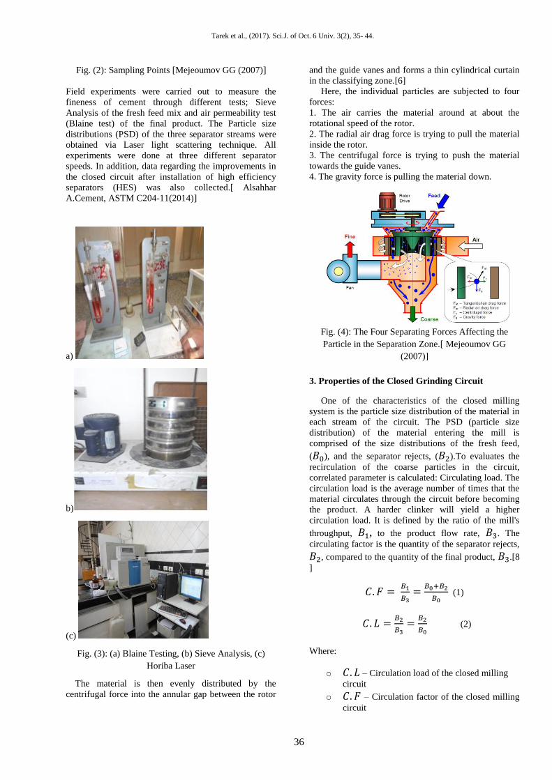
Fig. (2): Sampling Points [Mejeoumov GG (2007)]
Field experiments were carried out to measure the
fineness of cement through different tests; Sieve
Analysis of the fresh feed mix and air permeability test
(Blaine test) of the final product. The Particle size
distributions (PSD) of the three separator streams were
obtained via Laser light scattering technique. All
experiments were done at three different separator
speeds. In addition, data regarding the improvements in
the closed circuit after installation of high efficiency
separators (HES) was also collected.[ Alsahhar
A.Cement, ASTM C204-11(2014)]
a)
b)
(c)
Fig. (3): (a) Blaine Testing, (b) Sieve Analysis, (c)
Horiba Laser
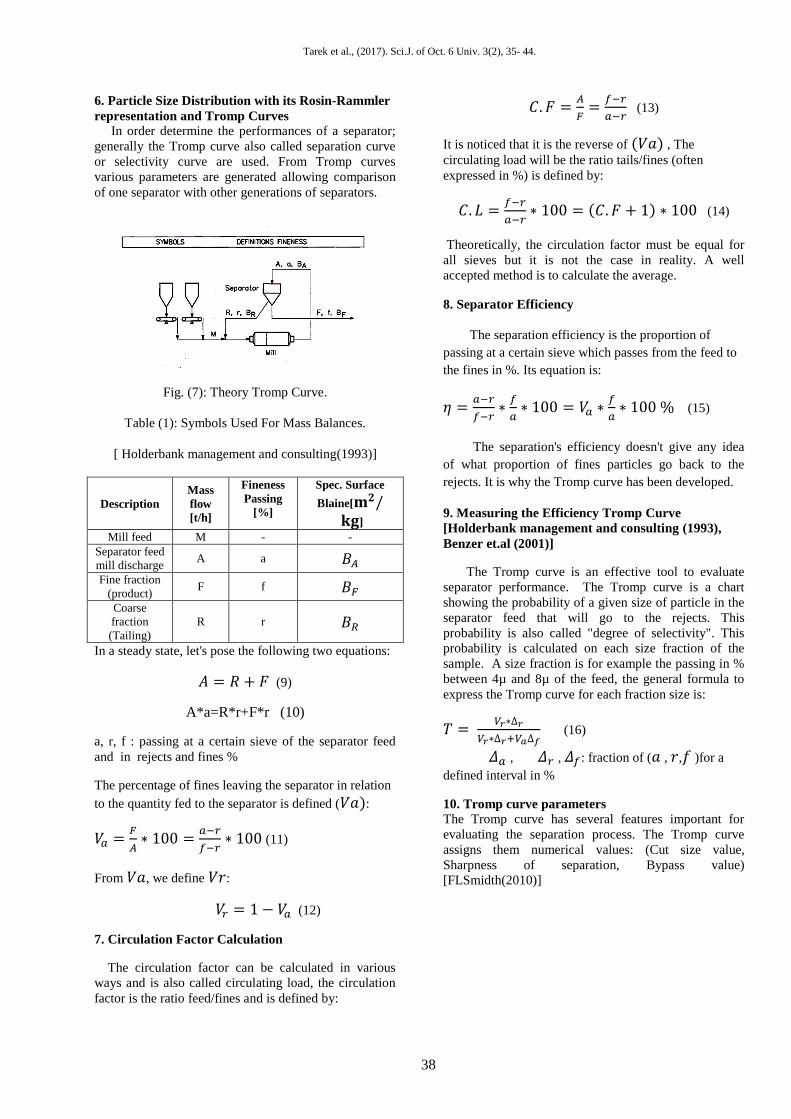
The material is then evenly distributed by the
centrifugal force into the annular gap between the rotor
and the guide vanes and forms a thin cylindrical curtain
in the classifying zone.[6]
Here, the individual particles are subjected to four
forces:
1. The air carries the material around at about the
rotational speed of the rotor.
2. The radial air drag force is trying to pull the material
inside the rotor.
3. The centrifugal force is trying to push the material
towards the guide vanes.
4. The gravity force is pulling the material down.
Fig. (4): The Four Separating Forces Affecting the
Particle in the Separation Zone.[ Mejeoumov GG
(2007)]
3. Properties of the Closed Grinding Circuit
One of the characteristics of the closed milling
system is the particle size distribution of the material in
each stream of the circuit. The PSD (particle size
distribution) of the material entering the mill is
comprised of the size distributions of the fresh feed,
(𝐵0), and the separator rejects, (𝐵2).To evaluates the
recirculation of the coarse particles in the circuit,
correlated parameter is calculated: Circulating load. The
circulation load is the average number of times that the
material circulates through the circuit before becoming
the product. A harder clinker will yield a higher
circulation load. It is defined by the ratio of the mill's
throughput, 𝐵1, to the product flow rate, 𝐵3. The
circulating factor is the quantity of the separator rejects,
𝐵2, compared to the quantity of the final product, 𝐵3.[8
]
𝐶. 𝐹 = 𝐵1
𝐵3=
𝐵0+𝐵2
𝐵0 (1)
𝐶. 𝐿 =𝐵2
𝐵3=
𝐵2
𝐵0 (2)
Where:
o 𝐶. 𝐿 – Circulation load of the closed milling
circuit
o 𝐶. 𝐹 – Circulation factor of the closed milling
circuit
36

Tarek et al., (2017). Sci.J. of Oct. 6 Univ. 3(2), 35- 44.
It also should be noted that the circulation load can
be calculated for each individual fraction determined by
the laser particle size analyzer using separator material
PSD data, expressed in the form of the individual
retained functions, 𝑓(𝑥).
𝐶. 𝐿𝑖 =𝐵1
𝐵3=
𝑓3𝑖−𝑓2𝑖
𝑓1𝑖−𝑓2𝑖 (3)
𝐶. 𝐿𝑖– Circulation load of the 𝑖-𝑡ℎ fraction.
4. Measuring of the Efficiency of Separation
The three material streams surrounding the separator
are:
1. Feed 2. Reject 3. Fine material [7]
Fig. (5): Material Streams Surrounding the Separator. [ Cement and Mining Processing (CMP)AG;2010]
The classifier splits up the feed material into two
separate streams: rejects and fines. All three material
streams are characterized by their individual mass flow
rate, B, and particle size distribution, 𝑓(𝑥). the typical
PSD data describing the three material streams
surrounding the HES are shown in Fig. (6).
(a)
(b)
Fig. (6): PSD of the Material Streams Surrounding
Separator (a – Cumulative Passing PSD; b – Individual
Retained PSD).[9,8]
In order to evaluate efficiency of the separation
process, the Tromp curve of the separator is calculated
and widely used throughout the cement industry. The
Tromp curve shows percent of the material in each
individual size fraction that is recovered into the coarse
stream. The opposite of the Tromp curve is the grade
efficiency curve (GEC), which defines percent of the
material in each fraction recovered into the fine stream.
[Mizonov et.al (1997), Bhattyet.al (2004)]
5. The Tromp Curve [Bhattyet.al (2004)]
The Tromp curve can be derived from the basic
principle of mass balance: The amount of material
supplied to the separator is equal to the amount of
material leaving it. In a steady-state operation, the mass
flow of the fresh feed is equal to the sum of mass flows
of fine and coarse streams.
𝐵1 = 𝐵2 + 𝐵3 (4)
Where:
𝐵1 , 𝐵2 , 𝐵3 Mass flow of the feed and coarse and fine
streams, mass per time unit.
𝐵1 . 𝑓1𝑖 = 𝐵2 . 𝑓2𝑖 + 𝐵3 . 𝑓3𝑖 (5)
Where:
𝑓1𝑖, 𝑓2𝑖 , 𝑓3𝑖 : Portion of the material in the i-th fraction
of the feed and coarse and fine streams.
The Tromp value for the 𝒊 − 𝒕𝒉 fraction is defined
by the probability of the feed particles to occur in the
coarse stream and equals the ratio of the coarse fraction
mass to the feed fraction mass.
𝑇𝑟𝑜𝑚𝑝𝑖 =𝐵2 .𝑓2𝑖
𝐵1 .𝑓1𝑖 (6)
Tromp curve is defined as:
𝑇𝑟𝑜𝑚𝑝 𝐶𝑢𝑟𝑣𝑒 =𝑓2𝑖
𝑓1𝑖 .
𝑓1𝑖−𝑓3𝑖
𝑓2𝑖−𝑓3𝑖 (7)
Grade Efficiency Curve is then defined by:
𝐺𝐸𝐶 =𝑓3𝑖
𝑓1𝑖 .
𝑓1𝑖−𝑓2𝑖
𝑓3𝑖−𝑓2𝑖 (8)
37
Tarek et al., (2017). Sci.J. of Oct. 6 Univ. 3(2), 35- 44.
6. Particle Size Distribution with its Rosin-Rammler
representation and Tromp Curves
In order determine the performances of a separator;
generally the Tromp curve also called separation curve
or selectivity curve are used. From Tromp curves
various parameters are generated allowing comparison
of one separator with other generations of separators.
Fig. (7): Theory Tromp Curve.
Table (1): Symbols Used For Mass Balances.
[ Holderbank management and consulting(1993)]
Description
Mass
flow
[t/h]
Fineness
Passing
[%]
Spec. Surface
Blaine[𝐦𝟐/ 𝐤𝐠]
Mill feed M - -
Separator feed
mill discharge A a 𝐵𝐴
Fine fraction
(product) F f 𝐵𝐹
Coarse
fraction
(Tailing)
R r 𝐵𝑅
In a steady state, let's pose the following two equations:
𝐴 = 𝑅 + 𝐹 (9)
A*a=R*r+F*r (10)
a, r, f : passing at a certain sieve of the separator feed
and in rejects and fines %
The percentage of fines leaving the separator in relation
to the quantity fed to the separator is defined (𝑉𝑎):
𝑉𝑎 =𝐹
𝐴∗ 100 =
𝑎−𝑟
𝑓−𝑟∗ 100 (11)
From 𝑉𝑎, we define 𝑉𝑟:
𝑉𝑟 = 1 − 𝑉𝑎 (12)
7. Circulation Factor Calculation
The circulation factor can be calculated in various
ways and is also called circulating load, the circulation
factor is the ratio feed/fines and is defined by:
𝐶. 𝐹 =𝐴
𝐹=
𝑓−𝑟
𝑎−𝑟 (13)
It is noticed that it is the reverse of (𝑉𝑎) , The
circulating load will be the ratio tails/fines (often
expressed in %) is defined by:
𝐶. 𝐿 =𝑓−𝑟
𝑎−𝑟∗ 100 = (𝐶. 𝐹 + 1) ∗ 100 (14)
Theoretically, the circulation factor must be equal for
all sieves but it is not the case in reality. A well
accepted method is to calculate the average.
8. Separator Efficiency
The separation efficiency is the proportion of
passing at a certain sieve which passes from the feed to
the fines in %. Its equation is:
𝜂 =𝑎−𝑟
𝑓−𝑟∗
𝑓
𝑎∗ 100 = 𝑉𝑎 ∗
𝑓
𝑎∗ 100 % (15)
The separation's efficiency doesn't give any idea
of what proportion of fines particles go back to the
rejects. It is why the Tromp curve has been developed.
9. Measuring the Efficiency Tromp Curve
[Holderbank management and consulting (1993), Benzer et.al (2001)]
The Tromp curve is an effective tool to evaluate
separator performance. The Tromp curve is a chart
showing the probability of a given size of particle in the
separator feed that will go to the rejects. This
probability is also called "degree of selectivity". This
probability is calculated on each size fraction of the
sample. A size fraction is for example the passing in %
between 4µ and 8µ of the feed, the general formula to
express the Tromp curve for each fraction size is:
𝑇 = 𝑉𝑟∗∆𝑟
𝑉𝑟∗∆𝑟+𝑉𝑎∆𝑓 (16)
𝛥𝑎 , 𝛥𝑟 , 𝛥𝑓: fraction of (𝑎 ,
𝑟,𝑓
)for a
defined interval in %
10. Tromp curve parameters
The Tromp curve has several features important for
evaluating the separation process. The Tromp curve
assigns them numerical values: (Cut size value,
Sharpness of separation, Bypass value)
[FLSmidth(2010)]
38

Tarek et al., (2017). Sci.J. of Oct. 6 Univ. 3(2), 35- 44.
Fig. 9: Tromp Curve Parameters [Benzer et.al (2001)]
Fig. 10: Cut Size [Benzer et.al (2001)]
1- The cut size d50 corresponds to 50% of the
feed passing to the coarse stream as see in Fig.
(10). It is therefore that size which has equal
probability of passing to either coarse or fine
streams.
2- sharpness of separation
The sharpness of separation of is defined as
follows:
𝑆ℎ =𝑑75
𝑑25 (17)
Where:𝑑25 And 𝑑75 – Particle sizes with Tromp
values of 25% and 75%. (An ideal separator has a 𝑆ℎ
of 1). [14] (Fig. 11)
Fig. 11: The Sharpness of Separation
Fig. 12: The bypass value
3- By –pass
The bypass value defines the portion of the material that
bypasses the classifying action. It is the part of the feed
that reports to the coarse stream independently of its
particle size due to agglomeration of the fine particles.
Therefore, it is immediately returned to the finish mill
with the rejected material. [Holderbank management
and consulting (1993), Benzer et.al (2001]
D limit (Limit dimension):
On the left of this point, the curve rises again. It means
that there is no more selective separation below D limit.
The high-raised "tail" to the left of the minimum of the
Tromp curve shown in (Fig. 13) is another consequence
of agglomeration of the fine particles and called the
"fish-hook" effect .Due to the frictional nature of
grinding in the second compartment of the mill, the
electrostatic charges are imposed upon the particles
leaving the mill. The smaller (lighter) particles are more
susceptible to the electrostatic forces and tend to coat
larger particles and/or stick together, forming
agglomerates.
11. Imperfection Factor [Bhattyet.al (2004)]
The imperfection factor gives an excellent idea of the
separator behavior. It is also good to compare between
separators. It is given by the following formula:
𝐼 =𝑑75−𝑑25
2∗𝑑50 (18)
Where: 𝒅𝟕𝟓, 𝒅𝟓𝟎 is and 𝒅𝟐𝟓 are the dimensions in
µm at 75%, 50% and 25% in the y-axis of the curve. It
should be as small as possible. Usual Fig.s and grades:
I < 0,2
Excellent separator
0,2 < I < 0,3
Good separator
0,3 < I < 0,4
Normal separator
0,4 < I < 0,6
Poor separator
0,6 < I < 0,7
Bad separator
I > 0,7
Execrable separator
The agglomerates are treated by the separator as
particles of larger size and have a higher probability of
passing into the coarse stream. Grinding aids help to
reduce agglomeration by relieving some of the
electrostatic charges imposed upon the particles and
thus improve recovery of the fine particles into the
product stream. The efficiency of the classification
process can be assessed by comparing the real life
39

Tarek et al., (2017). Sci.J. of Oct. 6 Univ. 3(2), 35- 44.
separator (Fig.13) to that of an ideal one. The ideal
separator would have a Tromp curve completely vertical
at the cut size, i.e., characterized by the sharpness of
separation 𝑆ℎ = 1 and, bypass=0.
(a) (b)
Fig. 13: (a) Tromp Curve of the High Efficiency
Separator , (b) Efficiency of the Separator Using Ideal
Tromp Curve.
All particles larger than the cut size would be sent to
rejects (Tromp = 100%), whereas all particles smaller
than the cut size would be recovered into the final
product (Tromp = 0%) – See Fig. (14) the ratio of the
areas under the Tromp curves of the real and ideal
separators defines the separation efficiency.
The cut size is commonly defined as the particle size at
which there is equal probability of the feed passing to
either the coarse or fine streams. The ideal cut size is
between 25 and 30 microns. The sharpness of cut is
measured by the ratio of (𝑑75/𝑑25). The nearer the
ratio is to 1.0, the sharper the separation.
An additional but less important feature is the ‘fish
hook effect’ commonly seen in classification curves. It
is associated with the finer particles and shows the
degree of return of fine particles to the coarse stream.
The following factors may cause this effect:
Larger particles are coated with finer
particles.
Incomplete feed dispersion.
Fines are entrained in the rejects.
Aggregations of fine particles that pass into
the coarse stream.
It needs to be remembered that the Tromp curve is an
indication of how the separator is working and not an
indication of the entire mill system
12. Tromp Curve Reduced
On the left of the D limit, the finest particles are
following the flow and are split between the rejects and
the fines in a total incertitude. There is no more
separation in this zone. In order to remove the effect of
that zone, the Tromp curve is reduced by the following
equation Fig. (15)
𝑇𝑟 =𝑇−𝐵𝑝
1−𝐵𝑝 (19)
𝑇𝑟 = Tromp reduced, 𝐵𝑝 = By-pass [8]
Fig. (15): Tromp Curve Reduced
13. The Markov chain theory was introduced to
describe the processes of grinding, classification, and
particle transport in a closed finish mill circuit. It was
utilized to allow calculation of all parameters of
continuous grinding process in a mill.
Using the identified Markov chain model, the ideal
grade efficiency curve was simulated and analyzed.
Simulation showed that PSD followed the shape of ideal
separation, the specific surface area increased and the
calculated 45-μm sieve passing value was 100%
indicating that all the final product was finer than the
cut size.
14. Results and Discussion
Table (2): Comparison of the (Production Rate, Energy
Consumption and Blaine Value) Before and After
Installation of a High Efficiency Separator
Cement
Mill System
Production
rate
[𝒕𝒐𝒏 / 𝒉]
Energy
consumption
[𝒌. 𝑾. 𝒉 / 𝒕𝒐𝒏]
Blaine
value
[𝒎𝟐 / 𝒌𝒈]
Ball Mill
Open Circuit 90- 100 60 310-320
Closed
Circuit
With(high
Efficiency
Separator)
110-130 42-48 350-380
40

Tarek et al., (2017). Sci.J. of Oct. 6 Univ. 3(2), 35- 44.
The results of the field experiments showed that all the
fineness indicating and Tromp curve parameters were
consistent with the testing conditions , also the separator
showed normal separation at all speeds. The data
collected showed that installation of high efficiency
separators improved the production rate and quality and
decreased the energy consumption. Results of the field
experiment were then utilized to identify the model's
parameters.
Table (3): Lab Blaine Results at different Separator
Speeds
Separator speed Lab Blaine [𝒎𝟐/𝒌𝒈]
High speed 396
Normal speed 381
Low speed 359
Results of the lab Blaine surface values showed the
highest values for the high separator speed and the
lowest values for the low separator speed. This was
consistent with the testing conditions. The high
separator speed rejects coarser particles producing a
finer product. The finer the product the higher the
surface area values (high Blaine results).
15. Efficiency of Separation: (A sampling campaign
gives the following results)
Size Efficiency % Tromp %
1 74.7 23.38
2 75.08 24.99
4 74.43 22.73
8 79.22 13.37
16 81.05 9.45
24 83.55 13.14
32 75.67 35.08
45 68.46 63.83
64 57.7 84.71
90 52.63 95.29
120 50.73 98.52
150 49.63 100
175 49.3 100
200 49.07 100
Fig. 16: Particle Size Distribution.
Fig. 17 : Efficiency of Separation
Fig. 18: Tromp Curve
Separator evaluation
Cut size (𝑑50%) 33.5µm this is a good estimation.
D limit: 12µm this is a rough estimation.
By-pass: 9 % this is a rough estimation
0
20
40
60
80
100
0 50 100 150 200 250
size
Efficiency %
Efficiency %
42
41
Tarek et al., (2017). Sci.J. of Oct. 6 Univ. 3(2), 35- 44.
Imperfection :With the formula: 𝐼 =𝑑75 %−𝑑25%
2∗𝑑50% 𝐼 =
47.1−24.3
2∗33.5 = 0.34
Sharpness factor (𝑺𝒉) = 𝑑75/𝑑25=47.1/24.3= 1.93
The sharpness of separation was the highest at the
normal separator speed (𝑆ℎ= 1.93), the higher
sharpness of separation value corresponds to a
narrower size range of particles. However, all
speeds showed sharpness ranging between (1.82-
1.93) which was close to the expected 2.0.
This separator has a Normal imperfection
indicating a normal separator behavior, the D limit
and the By-pass are satisfactory.
Although all separator speeds showed normal
behavior, but the bypass values were good (less
than 10%) at all separator speeds.
Table (4) :Tromp Curve Results
Tromp
curve
parameters
C.L
[%] 𝒅𝟐𝟓
[μm]
𝒅𝟓𝟎
[μm]
𝒅𝟕𝟓
[μm]
Sh
I
By
Pass
[%]
D
Limit
[μm]
High
separator
speed
74 24.5 33.4 46.6 1.90 0.33 5.8 12
Normal separator
speed
103 24.3 33.5 47.1 1.93 0.34 9.5 12
Low separator
speed
86 28.0 36.3 51.1 1.82 0.32 7.2 12
The separator behavior didn't change with the change
of the speed, in the low separator speed, Imperfection
(I)=0.32,for the normal speed (I)=0.34 and for the
high speed (I)=0.33. All separator speeds showed
Normal Separation.
The lower separator rotor speed rejects less coarse
particles; it yields a lower fineness of the final
product. On the other hand, higher separator rotor
speed rejects more course particles and leads to a
higher fineness of the final product, and that was
consistent with the results where the curve of the high
speed was shifted to the left towards the smaller
particle size and (lower𝑥50 ). Although the range
between different sizes was narrow but still, the
variable separator speed test revealed a definite
relationship between the separator rotor speed and the
fineness characteristics of the final product.
The smaller the cut size value, the finer the final
product, and that was consistent with the results
where:
- The high-speed separator showed the smallest cut size
value 𝑥50 =33.4𝜇𝑚 , while the normal speed
𝑥50 =33.5𝜇𝑚 and the low speed 𝑥50 =36.3𝜇𝑚 .
Although all separator speeds showed normal
behavior, but the bypass values were good (less than
10%) at all separator speeds.
16. Numerical Simulation and Analysis [12]
The Markov chain model was constructed and the
analysis of the finish mill grinding circuit was
performed using the MATLAB software.
17. Model Identification
For identification of the parameters of the Markov
chain model. The data obtained from the nominal
regime "Normal Speed – Normal Air" observed during
the experiment was used.The input variables of the
model were:
• 𝑄1(x), 𝑄2(x), 𝑄3(x), and 𝑄0(x)– Particle size
distributions in the cumulative percent passing form
describing the separator streams and fresh feed mixture
,( 𝐵0 ) Rate of the fresh feed to the entire circuit.[12]
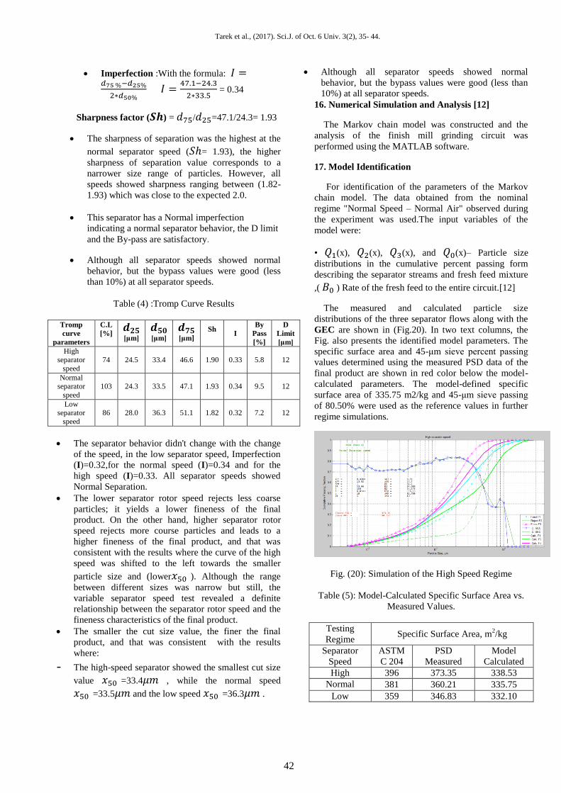
The measured and calculated particle size
distributions of the three separator flows along with the
GEC are shown in (Fig.20). In two text columns, the
Fig. also presents the identified model parameters. The
specific surface area and 45-μm sieve percent passing
values determined using the measured PSD data of the
final product are shown in red color below the model-
calculated parameters. The model-defined specific
surface area of 335.75 m2/kg and 45-μm sieve passing
of 80.50% were used as the reference values in further
regime simulations.
Fig. (20): Simulation of the High Speed Regime
Table (5): Model-Calculated Specific Surface Area vs.
Measured Values.
Testing
Regime Specific Surface Area, m
2/kg
Separator
Speed
ASTM
C 204
PSD
Measured
Model
Calculated
High 396 373.35 338.53
Normal 381 360.21 335.75
Low 359 346.83 332.10
42
Tarek et al., (2017). Sci.J. of Oct. 6 Univ. 3(2), 35- 44.
The performance characteristics of cement depend
not only on the specific surface area of the material, but
also on the proportion of the fine and coarse particles,
i.e., the shape of the PSD of cement. Therefore, the
model calculated and compared the shape of the PSD of
the fines at all the tested regimes: high, normal, and low
separator speeds as shown in (Fig. 20).
The model calculated PSD curves at the three tested
speeds showed a narrow range. The model calculated
PSD of the high speed was shifted to the left toward the
smaller particle sizes
18. Ideal Grade Efficiency Curve
The most desired property of any separator is to
have an efficiency of 100%. This means all particles
smaller than the cut size of the separator become final
product (none of the coarse particles become the final
product) and all particles larger than the cut size become
rejects (none of the fine particles escapes to the rejects
stream). The grade efficiency curve values of the ideal
separator are equal to 1 for all fractions less than 𝑥50
and 0 for fractions larger than 𝑥50.
The ideal grade efficiency curve can be simulated
using the Markov chain model. The particle size
distributions for the Normal Speed operating regime
would look like the following if the separator was ideal,
almost the entire PSD of the final product, 𝑄3(𝑥),
would lie below the cut size of the separator, 𝑥50 = 33.5
μm, whereas the PSD of the rejected material, 𝑄2(𝑥),
would be situated above the cut size. Since all the
particles of the final product would be finer than 33.5
μm, the 45-μm sieve passing value would be 100% and
the specific surface area of the product would increase
from 335.75 m2/kg of the real classification conditions
to 400.06 m2/kg of the ideal ones. (Fig.21)
Fig. (21): Simulation of the Ideal Classification.
The increase of the product's fineness level was
anticipated due to the following characteristic features
of the ideal GEC (or ideal Tromp curve): (Zero By
pass, Lack of the "fish-hook" effect, Unit sharpness of
separation)
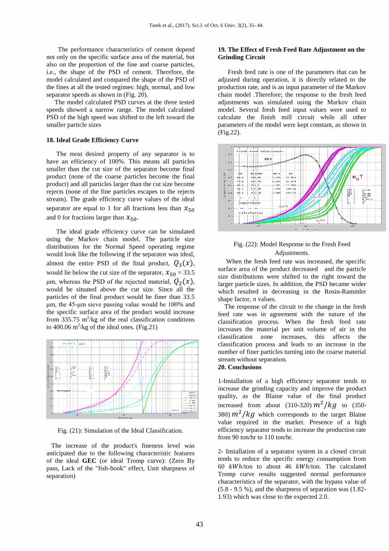
19. The Effect of Fresh Feed Rate Adjustment on the
Grinding Circuit
Fresh feed rate is one of the parameters that can be
adjusted during operation, it is directly related to the
production rate, and is an input parameter of the Markov
chain model .Therefore; the response to the fresh feed
adjustments was simulated using the Markov chain
model. Several fresh feed input values were used to
calculate the finish mill circuit while all other
parameters of the model were kept constant, as shown in
(Fig.22).
Fig. (22): Model Response to the Fresh Feed
Adjustments.
When the fresh feed rate was increased, the specific
surface area of the product decreased and the particle
size distributions were shifted to the right toward the
larger particle sizes. In addition, the PSD became wider
which resulted in decreasing in the Rosin-Rammler
shape factor, n values.
The response of the circuit to the change in the fresh
feed rate was in agreement with the nature of the
classification process. When the fresh feed rate
increases the material per unit volume of air in the
classification zone increases, this affects the
classification process and leads to an increase in the
number of finer particles turning into the coarse material
stream without separation.
20. Conclusions
1-Installation of a high efficiency separator tends to
increase the grinding capacity and improve the product
quality, as the Blaine value of the final product
increased from about (310-320) 𝑚2/𝑘𝑔 to (350-
380) 𝑚2/𝑘𝑔 which corresponds to the target Blaine
value required in the market. Presence of a high
efficiency separator tends to increase the production rate
from 90 ton/hr to 110 ton/hr.
2- Installation of a separator system in a closed circuit
tends to reduce the specific energy consumption from
60 𝑘𝑊ℎ/ton to about 46 𝑘𝑊ℎ/ton. The calculated
Tromp curve results suggested normal performance
characteristics of the separator, with the bypass value of
(5.8 - 9.5 %), and the sharpness of separation was (1.82-
1.93) which was close to the expected 2.0.
43

Tarek et al., (2017). Sci.J. of Oct. 6 Univ. 3(2), 35- 44.
3- Cement quality parameters affecting its performance
as a construction material were identified through the
Markov chain model; such as the specific surface area,
the percent passing through 45-μm sieve, and the
particle size distribution shape. The developed Markov
chain model simulated and analyzed the ideal grade
efficiency curve and the response to the changes in the
fresh feed rate. The effect on the specific surface area
and PSD shape of the final product was consistent with
the physical nature of the classification process.
References
1. Alsahhar A.Cement Tests. Material
labs[Internet].
2. ASTM (2014) C204-11.Standard test methods
for fineness of hydraulic cement by Air –
permeability Apparatus. [Internet]. West
Conshohocken PA: Serdar Aldanmazlar; Jan
24.
3. Benzer H, Ergun L, Lynch A , Oner M, Gunlu
A, Celik I (2001). Modeling cement grinding
circuits. Minerals Engineering; 14: 1469-1482.
4. Bhatty J, Miller F, Kosmatka S (2004).
Innovations in portland cement manufacturing,
CD-ROM: SP400, Portland Cement
Association, Skokie, IL,.
5. Cement and Mining Processing AG. CEMAG
High Efficiency Cross Flow-classifier
(2010).[Brochure].Germany: Cement and
Mining Processing (CMP)AG;
6. FLSmidth (2010). FLSmidth ball mill for
cement grinding.[Brochure].Denmark:
FLSmidth A/S;.
7. Holderbank management and consulting
.Cement engineering book-separators[Internet]
2000. available from:
8. Holderbank management and consulting.
Cement seminar process technology (
Operation of separators)
(1993).[Brochure].Switzerland: Holderbank .
9. Kawatra SK. (2006). Advances in
comminution.: Colorado. Society for Mining,
Metallurgy, and Exploration;2006.
10. Kohlhaas B.(1983) Cement Engineers'
Handbook, 4th
ed. Otto Labahn,
11. Mejeoumov GG (2007). Improved Cement
Quality and Grinding Efficiency by Means of
Closed Mill Circuit Modeling.Ph.D. Thesis.
Civil Engineering Department, Texas A&M
University.
12. Mizonov V, Berthiaux H, Zhukov V, Bernotat
S. Application of multidimensional Markov
chains to model kinetics of grinding with
internal classification. Int J Miner
Process 2004; 74S: S307-S315
13. Mizonov V, Zhukov V, Bernotat S. Simulation
of grinding: new approaches. Ivanovo State
Power Engineering University Press, Ivanovo,
Russia1997
14. T. k. Belhaj; Prof. Dr. M. G. Higazy; Ass. Prof.
A. M. Gaafer; and Dr. B. A. K. ELmogy
"Productivity Improvement for Cement
Industries",Ph.D. Thesis, Faculty of
Engineering,Shoubra,Mechanical Engnieering
Department, Benha University,2016.


