
Implementation of Active Noise Cancellation
in a Duct
by
Simranjit Sidhu
A Thesis Submitted In Partial Fulfillment of the
Requirements for the Degree of
Bachelor of Applied Science
in the
School of Engineering Science
Simranjit Sidhu 2013
SIMON FRASER UNIVERSITY
Fall 2013

ii

iii
Partial Copyright Licence

iv
Abstract
An Active Noise Cancellation (ANC) system is implemented in real time using both feed
forward LFXLMS (Leaky filtered-X least-mean-square) and feedback LFXLMS
approaches for adaptive filtering. ANC algorithms are implemented on a ADAU1446
evaluation board and tested in terms of sound cancellation in a duct. The hardware and
software interfaces required for the system are explained in detail. A Test bed is
developed to measure the performance of sound cancellation. Results are analysed in
detail and recommendations are made for future research work to improve the
performance of the system and to realize noise cancellation in 3D space.
Keywords: Active Noise Cancellation (ANC); ANC in a duct; feed forward FXLMS; feedback FXLMS; ADAU1446 DSP chip;

v
Dedication
This report is dedicated to my friends, family and mentor for all their support.

vi
Acknowledgements
I would like to thank my mentor, Dr. Ivan V. Bajić, for providing me this great opportunity,
guidance and feedback on regular basis during the project. I would also like to thank
Ms. Hanieh Khalilian, who is pursuing her Ph.D. at SFU, for sharing her knowledge on
adaptive filter theory. Last but not least, I would like to thank Mr. Eric Bujold, Senior
Principal Engineer at Broadcom Canada Ltd, for his advice on selection of real time
audio processing chip.

vii
Table of Contents
Approval ........................................................................... Error! Bookmark not defined. Partial Copyright Licence ............................................................................................... iii Abstract .......................................................................................................................... iv Dedication ....................................................................................................................... v Acknowledgements ........................................................................................................ vi Table of Contents .......................................................................................................... vii List of Tables .................................................................................................................. ix List of Figures.................................................................................................................. x List of Acronyms ............................................................................................................ xii Executive Summary ...................................................................................................... xiii
1. Introduction .......................................................................................................... 1
2. Background .......................................................................................................... 2 2.1. Adaptive Filters ....................................................................................................... 2
2.1.1. FIR Filter ..................................................................................................... 3 2.1.2. Adaptive Algorithms .................................................................................... 4
LMS Algorithm ............................................................................................ 5 How to choose the step size for basic LMS? ......................................... 6 Practical implementation considerations ................................................ 7
Leaky LMS Algorithm .................................................................................. 7 Practical implementation considerations ................................................ 8
Filtered-X LMS Algorithm ............................................................................ 8 How to choose the step size for FXLMS? .............................................. 9
2.2. Active Noise Cancellation Using the FXLMS Algorithm ........................................ 10 2.2.1. Feed forward topology for ANC ................................................................. 10 2.2.2. Feedback topology for ANC ...................................................................... 13 2.2.3. Simplifying feed forward and feedback ANC implementation .................... 14
3. Hardware Setup .................................................................................................. 15 3.1. DSP Processor (ADAU1446) ................................................................................ 15
3.1.1. Numeric format of the ADAU1446 DSP chip ............................................. 16 3.2. Audio Signal Chain ............................................................................................... 16
3.2.1. Front end of the audio signal chain ........................................................... 16 Microphone ............................................................................................... 16 Pre-amplifier ............................................................................................. 18 Preamp and microphone interface calculations ......................................... 19 Preamp and ADC interface calculations .................................................... 20
3.2.2. Back end of the audio signal chain ............................................................ 21 Power Amplifier ......................................................................................... 21 Speakers .................................................................................................. 21 Power amplifier and DAC interface ........................................................... 22 Power amplifier and speaker interface ...................................................... 22
3.3. Hardware pin connections for boards ................................................................... 22
viii
4. Software setup .................................................................................................... 24 4.1. Secondary path estimation ................................................................................... 24 4.2. Leaky FXLMS Adaptive Filter ............................................................................... 28
5. Test Bed .............................................................................................................. 30
6. Procedure for testing ......................................................................................... 32 6.1. Initial test setup procedure.................................................................................... 32 6.2. Testing ANC algorithms ........................................................................................ 34
7. Results and Discussion ..................................................................................... 37 7.1. Result of ANC by feed forward LFXLMS ............................................................... 37 7.2. Results of ANC by feedback LFXLMS .................................................................. 43
8. Conclusions ........................................................................................................ 50
9. Future Improvements ......................................................................................... 51
References ................................................................................................................... 54
Appendices .................................................................................................................. 56 Appendix A. Perl programs .................................................................................... 57 Appendix B. MATLAB programs ............................................................................ 58 Appendix C. Using the Eval-ADAU144xEBZ with SigmaStudio ............................. 62 Appendix D. FFmpeg for audio file conversion ...................................................... 69

ix
List of Tables
Table 1. ADAU1446 specifications (Analog Devices, 2013) ....................................... 15
Table 2. ADMP504 specifications (Analog Devices, 2013)......................................... 18
Table 3. SSM2167 specifications (Analog Devices, 2013) ......................................... 18
Table 4. Power amplifier specifications (Texas Instuments, 2012) ............................. 21
Table 5. Speaker specifications (Visaton, 2013) ........................................................ 22
Table 6. Sound suppression (in dB) at various frequencies using feed forward LFXLMS algorithm ....................................................................................... 41
Table 7. Sound suppression (in dB) at various frequencies using feedback LFXLMS algorithm ....................................................................................... 47

x
List of Figures
Figure 1. Physical idea of ANC (Wikibooks, 2012) ........................................................ 2
Figure 2. Block diagram of an adaptive filter. ................................................................ 3
Figure 3. Time-varying FIR filter (adapted from Kuo and Lee, 2001). ............................ 4
Figure 4. Block diagram of ANC using FXLMS algorithm (adapted from Kuo and Morgan, 1999) ............................................................................................... 9
Figure 5. Feed forward leaky FXLMS topology for ANC .............................................. 11
Figure 6. Feedback-neutralisation feed forward leaky FXLMS topology for ANC ........ 12
Figure 7. Feedback leaky FXLMS topology for ANC ................................................... 13
Figure 8. Audio Signal Chain (Lewis J. , Common Inter IC digital interface for audio data transfer) ...................................................................................... 16
Figure 9. Hardware pin connections ............................................................................ 23
Figure 10. Estimation of secondary path transfer function ............................................. 25
Figure 11. Group delay of the secondary path transfer function at the sampling rate of 24kHz. .............................................................................................. 27
Figure 12. Magnitude and phase plot of secondary path transfer function at the sampling rate of 24kHz. ............................................................................... 28
Figure 13. Wood-frame ANC test bed ........................................................................... 30
Figure 14. Inside view of the wooden duct. ................................................................... 31
Figure 15. Basic sine wave capture test. 500Hz sine wave is generated on the ADAU1446 board at the sampling rate of 24000Hz. The same wave is captured by a laptop microphone input at the sampling rate of 44100Hz. ..................................................................................................... 34
Figure 16. ANC result for demoFeedforwardLeakyFxLMS107taps.dspproj, with sine wave noise of 500Hz generated from board at sampling frequency = 24 kHz. ..................................................................................... 36
Figure 17. Comparison of power spectra with and without ANC at 800Hz..................... 38
Figure 18. Comparison of power spectra with and without ANC at 800Hz. The graph is magnified around 800Hz. ............................................................... 38
Figure 19. Comparison of power spectra with and without ANC at 7000Hz ................... 39

xi
Figure 20. Comparison of power spectra with and without ANC at 7000Hz. The graph is magnified around 7000Hz. ............................................................. 39
Figure 21. Comparison of power spectra with and without ANC at 3000Hz ................... 40
Figure 22. Comparison of power spectra with and without ANC at 3000Hz. The graph is magnified around 3000Hz. ............................................................. 40
Figure 23. Noise reduction vs. frequency for ANC using feed forward adaptive filter. Red line shows the overall trend of noise reduction. ........................... 42
Figure 24. Compare white noise power spectrum with ANC and without ANC for feed forward adaptive filter. .......................................................................... 43
Figure 25. Comparison of power spectra with and without ANC at 300Hz. .................... 44
Figure 26. Comparison of power spectra with and without ANC at 300Hz. The graph is magnified around 300Hz. ............................................................... 44
Figure 27. Comparison of power spectra with and without ANC at 500Hz..................... 45
Figure 28. Comparison of power spectra with and without ANC at 500Hz. The graph is magnified around 500Hz. ............................................................... 45
Figure 29. Comparison of power spectra with and without ANC at 5000Hz. .................. 46
Figure 30. Comparison of power spectra with and without ANC at 5000Hz. The graph is magnified around 5000Hz. ............................................................. 46
Figure 31. Plot noise reduction verses frequency for feedback adaptive filter. Red line shows the overall trend of noise reduction. .................................... 48
Figure 32. Comparison of white noise power spectra with and without ANC using feedback adaptive filter. ............................................................................... 49
Figure 33. Fully digital audio signal chain (Lewis J. , Common Inter IC digital interface for audio data transfer) .................................................................. 52
Figure 34. Feed forward adaptive filter approach with no error microphone .................. 53

xii
List of Acronyms
ANC Active Noise Cancellation
DSP Digital Signal Processing
ECM Electret Condenser Microphone
FFT Fast Fourier Transform
FIR Finite Impulse Response filter
FXLMS Filtered-X Least Mean Square
LFXLMS Leaky Filtered-X Least Mean Square
LMS Least Mean Square
MEMS Micro-Electro-Mechanical System
MMACs Million Multiply Accumulate Cycles per second
NLMS Normalised Least Mean Square
SPL Sound Pressure Level
xiii
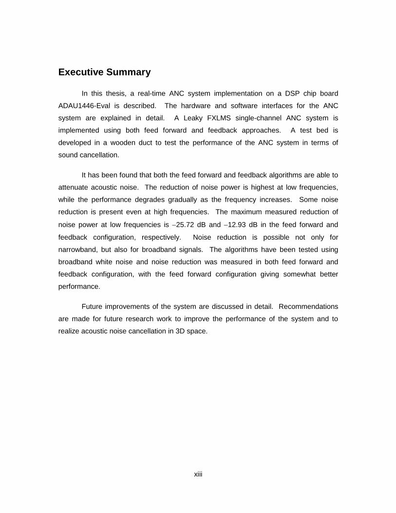
Executive Summary
In this thesis, a real-time ANC system implementation on a DSP chip board
ADAU1446-Eval is described. The hardware and software interfaces for the ANC
system are explained in detail. A Leaky FXLMS single-channel ANC system is
implemented using both feed forward and feedback approaches. A test bed is
developed in a wooden duct to test the performance of the ANC system in terms of
sound cancellation.
It has been found that both the feed forward and feedback algorithms are able to
attenuate acoustic noise. The reduction of noise power is highest at low frequencies,
while the performance degrades gradually as the frequency increases. Some noise
reduction is present even at high frequencies. The maximum measured reduction of
noise power at low frequencies is 25.72 dB and 12.93 dB in the feed forward and
feedback configuration, respectively. Noise reduction is possible not only for
narrowband, but also for broadband signals. The algorithms have been tested using
broadband white noise and noise reduction was measured in both feed forward and
feedback configuration, with the feed forward configuration giving somewhat better
performance.
Future improvements of the system are discussed in detail. Recommendations
are made for future research work to improve the performance of the system and to
realize acoustic noise cancellation in 3D space.

1
1. Introduction
Acoustic noise problems are ever increasing. Passive noise control and active
noise cancellation (ANC) are the two main techniques to reduce noise. Passive noise
control is the traditional approach, relying on noise-absorbing materials like foam sheets,
noise-absorbing tiles, insulation sheets, etc., to prevent the noise from entering the area
of interest. Passive noise control is very effective in suppressing high-frequency noise,
but it becomes cumbersome, costly and inefficient at low frequencies. On the other
hand, ANC is thought to be effective for reducing low-frequency noise.
Although the concept of ANC has been around for more than seventy five years
(Lueg, 1936), ANC is still an active and important research topic because of its wide
range of applications, some of which include:
Reducing noise from motors, heavy machinery and engines, etc.
Providing quiet environment in automobile and aeroplane cabins, etc.
High-end headphone systems.
Reducing mechanical wear out and fuel consumption through vibration control.
Reducing background noise in communication systems e.g., radio communication systems used by helicopter/aircraft pilots, teleconference systems.
Quieting of submarines to reduce their possibility of detection by sonar.
This thesis first briefly describes some background theory of ANC and then
elaborates on a practical implementation of ANC for sound control in a duct.

2
2. Background
Active Noise Cancellation (ANC) is a technique to reduce the unwanted acoustic
noise by generating anti-noise sound through a noise-cancelling speaker. Anti-noise is a
sound wave with the same amplitude, but with inverted phase compared to the original
noise. The unwanted noise and anti-noise superimpose acoustically, resulting in
cancellation. The physical idea of ANC is shown in Figure 1 below.
+ =
Noise
Anti Noise
Residual Noise
Figure 1. Physical idea of ANC (Wikibooks, 2012)
The practical implementation of ANC is realized using adaptive filters. In next section,
the basic theory of adaptive filters and various algorithms used for their implementation
is discussed.
2.1. Adaptive Filters
Adaptive filters self-adjust their transfer function according to the adaptive
algorithm driven by the error signal. An Adaptive filter consists of two parts, a FIR (Finite
Impulse Response) filter and an adaptive algorithm that will constantly update the

3
coefficients of the FIR filter. The block diagram of an adaptive filter is shown in Figure 2
below.
Noise Signal
Adaptive algorithm
Digital FIR Filter
Anti Noise Signal
+ =
x(n)
y(n)
e(n)
d(n)
- y(n)
Signal Inverter
- y(n)
Reference Mic
Error MicNoise Cancelling Speaker
Residual Noise
Figure 2. Block diagram of an adaptive filter.
In this figure, 𝑛 is the time index, 𝑑(𝑛) is the (un)desired noise signal to be canceled at
the summing junction, 𝑥(𝑛) is the reference noise signal captured at the reference
microphone, 𝑦(𝑛) is the output of the FIR filter, and 𝑒(𝑛) is the error signal captured at
the error microphone:
𝑒(𝑛) = 𝑑(𝑛) − 𝑦(𝑛). (1)
The adaptive algorithm will change the transfer function of the filter by updating the
coefficients of the FIR filter in a way that the error signal 𝑒(𝑛) is minimised on each
iteration.
2.1.1. FIR Filter
The FIR filter is usually realized as a tapped-delay line. The input signal is
delayed by as many time units as there are filter coefficients. The delayed signal path is

4
"tapped" and the delayed signal samples are multiplied by FIR filter coefficients and
summed up at the output.
The structure of an 𝐿-tap time-varying FIR filter is shown in Figure 3 below.
Figure 3. Time-varying FIR filter (adapted from Kuo and Lee, 2001).
In this figure, 𝑤0(𝑛), 𝑤1(𝑛), … , 𝑤𝐿−1(𝑛) are the 𝐿 FIR filter coefficients. The time index 𝑛
indicates that the filter coefficients change with time. The sequence of delayed input
samples is represented as 𝑥(𝑛), 𝑥(𝑛 − 1), … , 𝑥(𝑛 − 𝐿 + 1). The output 𝑦(𝑛) is given by
𝑦(𝑛) = ∑ 𝑤𝑚(𝑛)𝑥(𝑛 − 𝑚)
𝐿−1
𝑚=0
. (2)
The input samples and FIR coefficients can be written as a vector, 𝐱(𝑛) = [𝑥(𝑛), 𝑥(𝑛 −
1), … , 𝑥(𝑛 − 𝐿 + 1)]𝑇 and 𝐰(𝑛) = [𝑤0(𝑛), 𝑤1(𝑛), … , 𝑤𝐿−1(𝑛)]𝑇 respectively, then equation
(2) can be represented in a more compact matrix-vector notation as
𝑦(𝑛) = 𝐰(𝑛)𝑇𝐱(𝑛). (3)
2.1.2. Adaptive Algorithms
The adaptive algorithm updates the filter coefficients on each iteration, so that
the filter output 𝑦(𝑛) gets closer to the (un)desired noise signal 𝑑(𝑛). In other words, the

5
error 𝑒(𝑛) is reduced on each iteration. One of the very basic adaptive algorithms is
least mean squares (LMS) algorithm.
LMS Algorithm
The Least Mean Squares (LMS) algorithm is a type of adaptive algorithm whose
goal is to find filter coefficients such that the mean square value of the error signal is
minimised. The LMS algorithm is based on the steepest descendent method from
numerical optimisation (Boyd and Vandenberghe, 2004) where the cost function is the
squared error signal 𝐽(𝑛) = 𝑒2(𝑛).
Following (Mathews and Douglas, 2003), the update equation for the FIR filter
coefficients will now be derived. First, note that the squared error 𝑒2(𝑛) is a function of
the filter coefficient vector 𝐰(𝑛) = [𝑤0(𝑛), 𝑤1(𝑛), … , 𝑤𝐿−1(𝑛)]𝑇 so it can be imagined as a
surface in an 𝐿-dimensional space whose coordinates correspond to the filter
coefficients. The gradient vector of this squared error surface is given by
∇𝐽(𝑛) = ∇𝑒2(𝑛) =𝜕𝑒2(𝑛)
𝜕𝐰(𝑛)= 2𝑒(𝑛)
𝜕𝑒(𝑛)
𝜕𝐰(𝑛)
= 2𝑒(𝑛) ∙ [𝜕𝑒(𝑛)
𝜕𝑤0(𝑛),
𝜕𝑒(𝑛)
𝜕𝑤1(𝑛), … ,
𝜕𝑒(𝑛)
𝜕𝑤𝐿−1(𝑛)]
𝑇
. (4)
The equation (5) is formed by using the fact that 𝑒(𝑛) = 𝑑(𝑛) − 𝑦(𝑛) = 𝑑(𝑛) − 𝐰(𝑛)𝑇𝐱(𝑛)
in the error gradient equation (4) above.
∇𝑒2(𝑛) = 2𝑒(𝑛)𝜕𝑒(𝑛)
𝜕𝐰(𝑛)= 2𝑒(𝑛)
𝜕
𝜕𝐰(𝑛)𝑑(𝑛) − 𝐰(𝑛)𝑇𝐱(𝑛) = −2𝑒(𝑛)𝐱(𝑛), (5)
where the final equality follows from the fact that the (un)desired noise signal 𝑑(𝑛) is not
a function of the filter coefficient vector 𝐰(𝑛), so 𝜕𝑑(𝑛)
𝜕𝐰(𝑛)= 𝟎.

6
The direction of the steepest descent of the squared error surface is given by the
negative gradient, that is, −∇𝑒2(𝑛) = 2𝑒(𝑛)𝐱(𝑛). Hence, in order to reduce the squared
error, the filter coefficient vector is updated as follows
𝐰(𝑛 + 1) = 𝐰(𝑛) + 𝜇𝑒(𝑛)𝐱(𝑛), (6)
where the factor 2 from the expression for the gradient has been bundled into the
coefficient 𝜇, known as the step size, which specifies how far in the direction of the
steepest descent has the coefficient vector moved.
It should be noted that due to the random nature of the input signals 𝑥(𝑛) and
𝑑(𝑛), the signals 𝑦(𝑛) and 𝑒(𝑛) in Figure 2 are also random. In this framework, the LMS
algorithm tries to update the filter coefficients in order to minimise the expected squared
error at the next time point 𝐸𝑒2(𝑛 + 1), and the expectation operator 𝐸∙ needs to be
applied throughout the above derivation. For simplicity, however, the derivation was
based on a simple one-sample estimate of the expected squared error at time 𝑛 + 1 as
the measured squared error at the current time 𝑛, that is, 𝐸𝑒2(𝑛 + 1) = 𝑒2(𝑛).
How to choose the step size for basic LMS?
The block diagram of the adaptive filter in Figure 2 shows that there is a
feedback loop from the error signal back to the adaptive algorithm block. The amount of
feedback depends upon the value of the step size 𝜇. The question is what range of
values for 𝜇 will ensure the convergence of the algorithm. It is shown in (Haykin, 2002)
and (Mathews and Douglas, 2003) that the appropriate range of values for 𝜇 is
0 < 𝜇 <2
𝐿𝜎𝑥2, (7)
where 𝐿 is the number of filter coefficients and 𝜎𝑥2 is the variance of the input signal 𝑥(𝑛),
sometimes also referred to as the signal energy or the signal power.
7
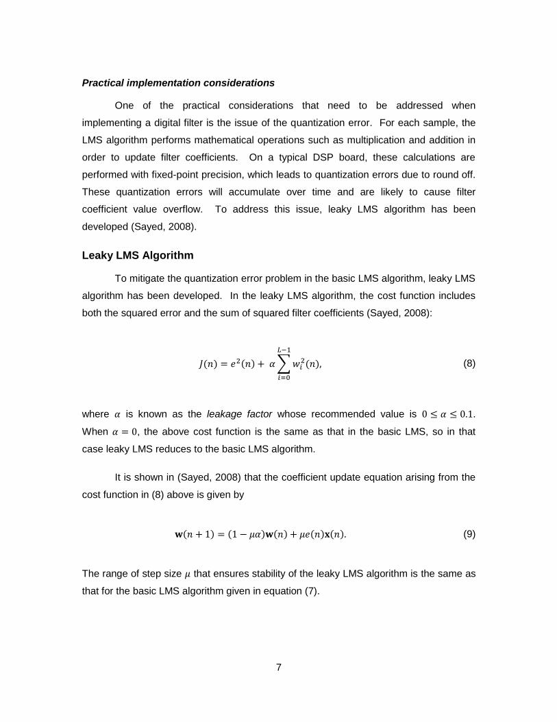
Practical implementation considerations
One of the practical considerations that need to be addressed when
implementing a digital filter is the issue of the quantization error. For each sample, the
LMS algorithm performs mathematical operations such as multiplication and addition in
order to update filter coefficients. On a typical DSP board, these calculations are
performed with fixed-point precision, which leads to quantization errors due to round off.
These quantization errors will accumulate over time and are likely to cause filter
coefficient value overflow. To address this issue, leaky LMS algorithm has been
developed (Sayed, 2008).
Leaky LMS Algorithm
To mitigate the quantization error problem in the basic LMS algorithm, leaky LMS
algorithm has been developed. In the leaky LMS algorithm, the cost function includes
both the squared error and the sum of squared filter coefficients (Sayed, 2008):
𝐽(𝑛) = 𝑒2(𝑛) + 𝛼 ∑ 𝑤𝑖2(𝑛)
𝐿−1
𝑖=0
, (8)
where 𝛼 is known as the leakage factor whose recommended value is 0 ≤ 𝛼 ≤ 0.1.
When 𝛼 = 0, the above cost function is the same as that in the basic LMS, so in that
case leaky LMS reduces to the basic LMS algorithm.
It is shown in (Sayed, 2008) that the coefficient update equation arising from the
cost function in (8) above is given by
𝐰(𝑛 + 1) = (1 − 𝜇𝛼)𝐰(𝑛) + 𝜇𝑒(𝑛)𝐱(𝑛). (9)
The range of step size 𝜇 that ensures stability of the leaky LMS algorithm is the same as
that for the basic LMS algorithm given in equation (7).

8
Practical implementation considerations
When either basic LMS or leaky LMS is used for ANC, the output of the filter,
𝑦(𝑛), is not applied directly to the summing junction, as shown in Figure 2. Rather, 𝑦(𝑛)
travels through the secondary path, which consists of a Digital-to-Analog Converter
(DAC), power amplifier, noise cancelling speaker, and the acoustic path from the noise
cancelling speaker to the summing junction, before reaching the summing junction. It is
obvious that the elements of the secondary path will introduce phase shift and other
distortions to 𝑦(𝑛), and the noise cancelling signal at the summing junction will be
different from the analog version of 𝑦(𝑛). For this reason, in order to accomplish
cancellation, it is important that that adaptive algorithm account for the secondary path
transfer function, as discussed next.
Filtered-X LMS Algorithm
The Filtered-X LMS (FXLMS) algorithm accounts for the effect of the secondary
path transfer function on the ANC system. The corresponding block diagram is shown in
Figure 4 below. In this diagram, various transfer functions are expressed in terms of the
𝑧-transform (Oppenheim and Willsky, 1996) of their impulse response. In this diagram,
the secondary path transfer function is represented as 𝑆(𝑧). There are two ways to
compensate for the effect of 𝑆(𝑧) in the ANC system.
The first solution is to apply the inverse filter 1/𝑆(𝑧) to the output of the adaptive
filter, shown as 𝑊(𝑧) in the diagram. This inverse filter will remove the effect of the
secondary path 𝑆(𝑧), since their combined transfer function is 𝑆(𝑧) ∙ 1 𝑆(𝑧)⁄ = 1.
However, this approach has a few drawbacks. First, it may happen that the inverse of
𝑆(𝑧) does not exist. Second, the inverse filter of an FIR filter, even if it exists, involves
inverse of a matrix which is more complex and would require a higher computational
cost (Kuo and Morgan, 1999).
The second solution, shown in Figure 4, is to place a filter identical to 𝑆(𝑧) in the
path of the reference noise signal 𝑥(𝑛) to the LMS weight update block. This way, the
signal entering the LMS block, denoted 𝑥′(𝑛), differs from the reference noise signal
𝑥(𝑛) in the same way that the signal entering the summing junction, denoted 𝑦′(𝑛)
differs from the output 𝑦(𝑛) of the adaptive filter. This will compensate the effect of

9
secondary path. The corresponding algorithm is known as Filtered-X LMS (FXLMS)
algorithm (Kuo and Morgan, 1999). If leaky LMS is employed in the LMS block instead
of the basic LMS, the resulting algorithm is known as the leaky Filtered-X LMS (leaky
FXLMS) algorithm.
Note that in Figure 4, 𝑃(𝑧) is the transfer function which models the acoustic path
from the reference microphone to the summing junction. If the reference noise signal
𝑥(𝑛) is provided as an input to the digital filter with transfer function 𝑃(𝑧), the output of
this filter will be the (un)desired noise signal 𝑑(𝑛) to be cancelled at summing junction.
Also note that the transfer function inserted into the reference signal path is (𝑧), the
estimate of 𝑆(𝑧), rather than 𝑆(𝑧) itself. This is because in practice the secondary path
transfer function is rarely known exactly, and needs to be estimated or measured
instead. In our test bed, 𝑆(𝑧) is measured offline, as explained in Section 4.1.
P(z)
S^(z)
W(z)
LMS
S(z)
x(n)
x’(n)
+
-y(n) y’(n)
d(n) e(n)
Figure 4. Block diagram of ANC using FXLMS algorithm (adapted from Kuo and Morgan, 1999)
How to choose the step size for FXLMS?
The weight update for FXLMS is the same as that for the basic LMS, given by
equation (6), with 𝐱(𝑛) replaced by 𝐱′(𝑛). Similarly, the weight update for leaky FXLMS
is the same as that for leaky LMS, given by equation (9), with 𝐱(𝑛) replaced by 𝐱′(𝑛).
However, the appropriate range of step size values is somewhat different compared to
LMS, and is given by

10
0 < 𝜇 <2
(𝐿 + ∆)𝜎𝑥2, (10)
where ∆ is the number of samples corresponding to the overall delay in the secondary
path (Kuo and Morgan, 1999). Since ∆ is a positive number, the upper bound on the
step size in (leaky) FXLMS is lower compared to the (leaky) LMS, hence the
convergence may be slower.
2.2. Active Noise Cancellation Using the FXLMS Algorithm
There are two implementation topologies for ANC using the FXLMS algorithm,
feed forward and feedback, both of which will be discussed next.
2.2.1. Feed forward topology for ANC
There are two feed forward structures that can be used for ANC using the
FXLMS algorithm. The first one is shown in Figure 5 below, and is essentially the same
as that shown in Figure 4. The reference noise signal 𝑥(𝑛) is measured by the
reference microphone, while the error signal 𝑒(𝑛) is measured by the error microphone.
In order to achieve subtraction at the summing junction, the output of the adaptive filter
𝑦(𝑛) has to be inverted to −𝑦(𝑛) before feeding it to the noise-cancelling speaker.

11
W(z)Weights of FIR
filter
Leaky LMSS^(z)
Estimation of secondary path
Noise Source
Reference Mic Error MicNoise Cancelling
Speaker
e(n)
x'(n)
x(n)
y(n)
FXLMS Adaptive Algorithm
Adaptive Filter
Signal Inverter
- y(n)
Figure 5. Feed forward leaky FXLMS topology for ANC
The above structure performs well if the reference microphone measures only
the reference noise signal 𝑥(𝑛). However, depending on the practical setup, the
reference microphone may also pick up a part of the signal from the noise cancelling
speaker, thereby creating another feedback loop in the system. The structure in Figure
5 can be modified as shown in Figure 6 to account for this feedback. The resulting
algorithm is known as feedback-neutralisation feed forward ANC approach.

12
W(z)Weights of FIR
filter
Leaky LMSS^(z)
Estimation of secondary path
Noise Source
Reference Mic Error MicNoise Cancelling
Speaker
e(n)
x'(n)
x(n)
y(n)
FXLMS Adaptive Algorithm
Adaptive Filter
Signal Inverter
- y(n)F(z)
+-
Figure 6. Feedback-neutralisation feed forward leaky FXLMS topology for ANC
In Figure 6, a new transfer function 𝐹(𝑧) is introduced between the noise-
cancelling signal −𝑦(𝑛) and the reference signal path. The transfer function 𝐹(𝑧) is
meant to approximate the effect of the acoustic feedback path between the noise-
cancelling speaker and the reference microphone. If 𝐹(𝑧) approximates this acoustic
path well, then subtracting the output of the 𝐹(𝑧) block from the reference microphone
signal will cancel the effect of the noise-cancelling sound picked up by the reference
microphone, thus leaving the reference noise signal 𝑥(𝑛) at the input to the adaptive
filter. Similarly to the secondary path transfer function 𝑆(𝑧), the acoustic feedback path
transfer function 𝐹(𝑧) is measured offline, as described in Section 4.1.
13
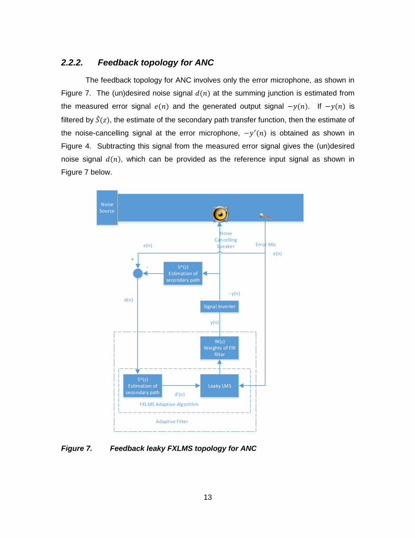
2.2.2. Feedback topology for ANC
The feedback topology for ANC involves only the error microphone, as shown in
Figure 7. The (un)desired noise signal 𝑑(𝑛) at the summing junction is estimated from
the measured error signal 𝑒(𝑛) and the generated output signal −𝑦(𝑛). If −𝑦(𝑛) is
filtered by (𝑧), the estimate of the secondary path transfer function, then the estimate of
the noise-cancelling signal at the error microphone, −𝑦′(𝑛) is obtained as shown in
Figure 4. Subtracting this signal from the measured error signal gives the (un)desired
noise signal 𝑑(𝑛), which can be provided as the reference input signal as shown in
Figure 7 below.
W(z)Weights of FIR
filter
Leaky LMSS^(z)
Estimation of secondary path
Noise Source
Error Mic
Noise Cancelling Speaker
e(n)
d'(n)
d(n)
y(n)
FXLMS Adaptive Algorithm
Adaptive Filter
S^(z)Estimation of
secondary path
e(n)
+
-
Signal Inverter
- y(n)
Figure 7. Feedback leaky FXLMS topology for ANC

14
2.2.3. Simplifying feed forward and feedback ANC implementation
The feed forward and feedback ANC based on leaky FXLMS can be simplified by
recognizing that the signal inverter is not needed if a simple modification is made to the
coefficient update equation. Note that the output of the adaptive filter will be −𝑦(𝑛),
without the inverter, if the reference noise signal is inverted from 𝑥(𝑛) to −𝑥(𝑛). This
inversion does not have to be done explicitly in the reference signal path. Instead, it can
be achieved in the coefficient update equation, by changing 𝐱(𝑛) to −𝐱(𝑛). This
modifies the leaky FXLMS coefficient update from equation (9) to the following:
𝐰(𝑛 + 1) = (1 − 𝜇𝛼)𝐰(𝑛) − 𝜇𝑒(𝑛)𝐱(𝑛). (11)
The ANC test bed described in the remainder of this thesis uses equation (11) for
adaptive filter coefficient update.
15
3. Hardware Setup
3.1. DSP Processor (ADAU1446)
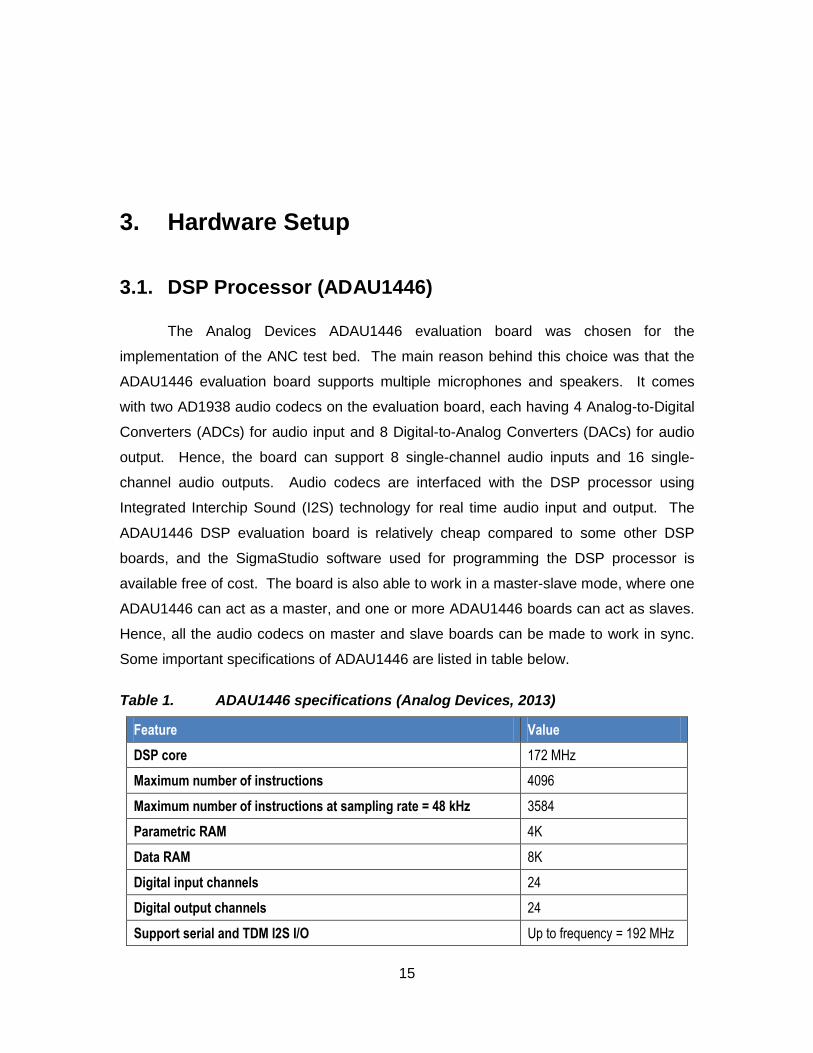
The Analog Devices ADAU1446 evaluation board was chosen for the
implementation of the ANC test bed. The main reason behind this choice was that the
ADAU1446 evaluation board supports multiple microphones and speakers. It comes
with two AD1938 audio codecs on the evaluation board, each having 4 Analog-to-Digital
Converters (ADCs) for audio input and 8 Digital-to-Analog Converters (DACs) for audio
output. Hence, the board can support 8 single-channel audio inputs and 16 single-
channel audio outputs. Audio codecs are interfaced with the DSP processor using
Integrated Interchip Sound (I2S) technology for real time audio input and output. The
ADAU1446 DSP evaluation board is relatively cheap compared to some other DSP
boards, and the SigmaStudio software used for programming the DSP processor is
available free of cost. The board is also able to work in a master-slave mode, where one
ADAU1446 can act as a master, and one or more ADAU1446 boards can act as slaves.
Hence, all the audio codecs on master and slave boards can be made to work in sync.
Some important specifications of ADAU1446 are listed in table below.
Table 1. ADAU1446 specifications (Analog Devices, 2013)
Feature Value
DSP core 172 MHz
Maximum number of instructions 4096
Maximum number of instructions at sampling rate = 48 kHz 3584
Parametric RAM 4K
Data RAM 8K
Digital input channels 24
Digital output channels 24
Support serial and TDM I2S I/O Up to frequency = 192 MHz

16
3.1.1. Numeric format of the ADAU1446 DSP chip
The ADAU1446 board uses fixed-point representation. According to (Analog
Devices wiki, 2013), the input to the DSP core on the ADAU1446 board is represented
with 24 bits. Inside the core, four additional bits are used, making the total number of
bits used for numeric representation equal to 28. Of these, 5 bits are used for the
integral part, and 23 bits are used for the fractional part, which is known as 5.23 format.
3.2. Audio Signal Chain
The audio signal chain is illustrated in Figure 8 below. The front end includes the
microphone, the preamp and the ADC, while the back end consists of the DAC, the
speaker amplifier (also known as power amplifier), and the speaker. The DSP chip is at
the center of the chain. The ADC, DSP chip, and DAC are already included on the
ADAU1446 board, while the remaining components need to be added separately and
interfaced to the board. Details are discussed next.
Figure 8. Audio Signal Chain (adapted from (Lewis, Common Inter IC digital interface for audio data transfer))
3.2.1. Front end of the audio signal chain
Microphone
Various types of microphones are available on the market. Some of the
important microphone characteristics for our ANC application are:
Low noise
Low power
ADAU 1446-Eval

17
Ability to form a microphone array
Easy access to the microphone datasheet and specifications
Easy interface with the ADAU1446 evaluation board
According to jeradL1, MEMS microphones have the following advantages over electret
microphones (ECM)
MEMS microphones have much better signal to noise ratio (SNR) than ECM
microphones for equivalent package size or volume. The ADMP504 MEMS
microphone has a 65 dB SNR in a 2.5 x 3.35 x 0.88 mm package (7.4 mm3),
while an ECM with similar performance may have a diameter of 9 mm and a 4
mm height, for a 254 mm3 volume.
MEMS microphones are less impacted by temperature changes as compared to
ECM microphones. The sensitivity of an ECM may drift as much as +/4 dB over
its operating temperature range, while a MEMS microphone's sensitivity may only
drift by 0.5 dB over the same range.
MEMS microphones are less sensitive to mechanical vibrations than ECM
microphone. It is because MEMS microphone's diaphragm is very light in weight
as compared to ECMs.
MEMS microphones of the same type can be easily arranged into microphone
array because of their identical frequency response. On the other hand, ECM
microphones of same type may have different frequency response, this
difference is more prominent at high and low frequencies.
MEMS microphones require less power as compared to ECMs
Based on our requirements for ANC and the various advantages provided by MEMS
microphones over electret microphones, the ultra-low noise ADMP504 MEMS
microphone was chosen for the test bed. Important specifications of the ADMP504
1 Analog Devices discussion board. http://ez.analog.com/message/42028

18
microphone are summarised in Table 2 below. Also note that the frequency response
range of ADMP504 microphone is approximately equal to the human hearing range
(20Hz – 20 kHz).
Table 2. ADMP504 specifications (Analog Devices, 2013)
Feature Value
Response Omnidirectional
SNR 65 dBA
Low current consumption <180 µA
Frequency response range 100 Hz to 20 kHz
Sensitivity 38 dBV
Pre-amplifier
The analog signal from the microphone is weak and cannot be directly fed to the
ADC. A Preamplifier is used to amplify the microphone signal. Choosing a correct
preamp for interfacing the microphone to the ADC converter requires knowledge of the
microphone, the ADC and preamp specifications. The SSM2167 preamp from analog
devices was selected. It is low noise voltage controlled amplifier (VCA). The amount of
amplification applied to the input signal depends upon the setting of the compression
ratio (which can be varied from 1:1 to 10:1) on the board. The chip also has a protection
mechanism so that signals above a certain threshold are limited (not amplified), which
prevents overloading the ADC. Moreover, for signals below a certain level the preamp
acts as a downward expander (noise gate) by attenuating background noise or hum in
the input signal. All these characteristics result in optimized signal levels prior to
digitization by ADC, and eliminates the need for additional gain or attenuation stage in
the system. (Analog Devices, 2013)
Table 3. SSM2167 specifications (Analog Devices, 2013)
Feature Value
Input voltage range 600 mV rms
Output voltage range 700 mV rms
VCA fixed gain 18 dB
VCA dynamic gain range 40 dB

19
Compression ratio minimum 1:1
Compression ratio maximum 10:1
Noise Gate settings 40 dBV, 48 dBV, 54 dBV, 55 dBV
Some calculations are presented in the next section to ensure that there is no
clipping of the analog signal in the front end of the audio signal chain. These
calculations will also give better understanding of the process of interfacing the
microphone, the preamp and the ADC in ANC hardware design.
Preamp and microphone interface calculations
One of the important characteristic of microphones is their sensitivity, which is
the magnitude of the analog electrical output signal for 1 kHz sine wave at the input
sound pressure of 1 Pascal2 (Lewis J. , Understanding Microphone Sensitivity, 2012).
Sensitivity is usually given in dBV3 units on the microphone datasheet. For example,
sensitivity of the ADMP504 microphone is 38 dBV. This means that if a 1 kHz sine
wave at 1 Pascal is given as an input sound signal to the ADMP504 microphone, the
output electrical signal will be 38 dBV.
The interface between the microphone and the preamp should avoid signal
clipping and overloading, i.e. the magnitude of the maximum output voltage of the
microphone should be less than the maximum input voltage of the preamp. Before
doing the interface calculations, it is worth mentioning that the maximum input voltage on
the preamp datasheets is in volts on a linear scale, while the maximum output voltage of
the microphone is provided usually in dBV on a logarithmic scale. The conversion of
dBV to the linear scale is shown next and it is used to determine the output of the
microphone in volts on the linear scale.
The relationship between the sensitivity in dBV units and the sensitivity in mV
units is shown in equation (12) below.
2 Pascal is a unit of pressure measurement. 1 Pascal = 94 dB sound pressure level. 3 dBV is voltage relative to 1 volt on logarithmic scale.

20
Sensitivity (dBV) = 20 log10 (SensitivitymV/Pa
OutputAREF
), (12)
where OutputAREF
is 1000 mV/Pa. Equation (12) can be rearranged in order to calculate
microphone sensitivity in mV on a linear scale as shown below.
SensitivitymV/Pa = (10−3820 ) ∙ 1000 = 12.5 mV at 94 dB SPL, (13)
where SPL stands for Sound Pressure Level.
As discussed above, the maximum output voltage signal on the linear scale from
the microphone is required in order to ensure no clipping of the input signal. This will
happen when the input sound signal is at maximum SPL handled by the microphone.
According to ADMP504 microphone specifications, the maximum SPL is 120 dB, which
is 26 dB above 94 dB (1 Pascal) SPL. This information can be used to calculate
microphone’s maximum output voltage signal at 120 dB as shown below
Maximum output voltage signal = (102620) ∙ 12.5 mV = 0.25 V. (14)
Hence, 0.25 V is the maximum input voltage for SSM2167 preamp. It is well below the
maximum input voltage for SSM2167, which is 0.60 V.
It is important to note that SSM2167 preamp by default is set up for an electret
microphone because it provides bias to an electret microphone by using a biasing
register of 2.2 kΩ. In order to use a MEMS microphone with SSM2167, this biasing
register should be de-soldered from the SSM2167 preamp board.
Preamp and ADC interface calculations
The microphone signal is very weak and should be amplified by a preamp before
feeding to ADC. The gain of the preamp should be set in such a way that the amplified
signal is never above the maximum input voltage of ADC.

21
The SSM2167 preamps have an elegant design. The input signals to SSM2167
preamp above a particular threshold level are not amplified. This feature allows the
preamp to limit the maximum output voltage signal (Analog Devices, 2013). From the
SSM2167 datasheet specifications, maximum output voltage is 0.70 V. This voltage is
within ADC full scale input voltage of 2 V and will not overload ADC.
3.2.2. Back end of the audio signal chain
The back end of the audio signal chain consists of the DAC, power amplifier and
speaker. This interface is simple compared to the front end. The reason is that the
power amplifier and speaker manufactures use the same language. Power amplifiers
are rated in output power (in Watts) for a given load (in Ohms), while speakers are rated
in impedance (in Ohms) with maximum power handling capacity (in Watts).
Power Amplifier
A pre-assembled and pre-tested power amplifier board (including power supply)
was selected for the test bed. The board uses Texas Instruments TPA3110 Class-D
stereo Audio Amplifier. According to the TPA3110 datasheet, the power efficiency is
close to 80% for 5 Watts of power output. Moreover, it dissipates less heat and no heat
sink is required. Some of the specifications are listed in Table 4 below.
Table 4. Power amplifier specifications (Texas Instuments, 2012)
Feature Value
Output power 5 W 2 @ 8 Ω
Frequency response 20 Hz to 20 kHz (+/ 3 dB)
Speakers
The speakers are made by Visaton. They are small in size and have
omnidirectional sound directivity pattern. These speakers can easily be arranged in a
speaker array because of their small size (diameter = 5 cm). The main specifications for
Visaton FRS 5-8 are listed in Table 5 below. Also note that the frequency response
range of Visaton FRS 5-8 speaker is approximately equal to the human hearing range
(20Hz – 20 kHz).
22
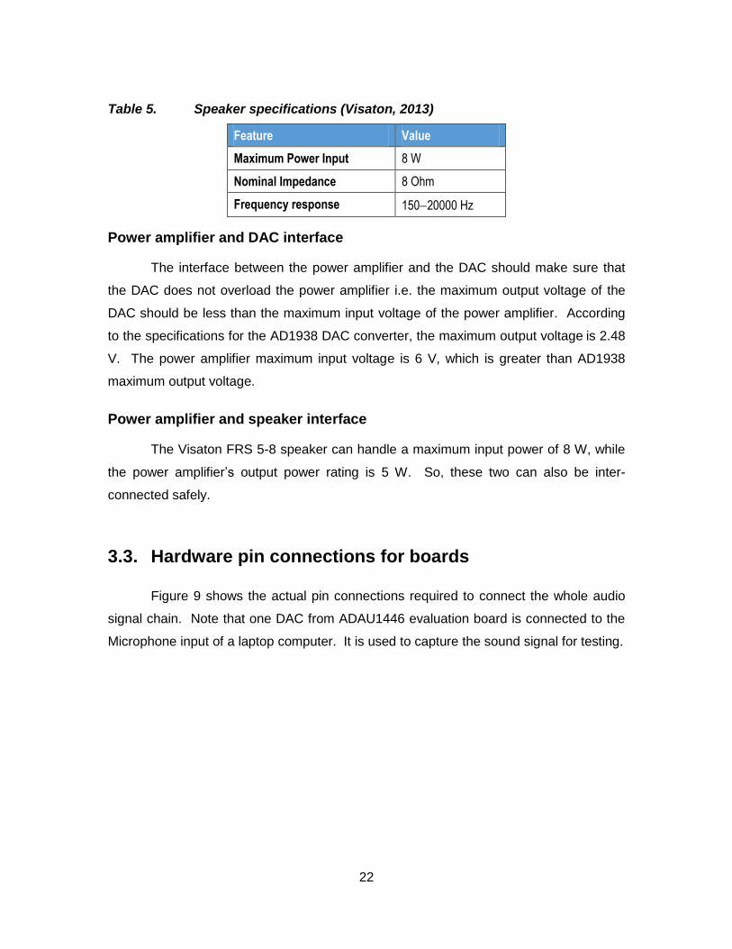
Table 5. Speaker specifications (Visaton, 2013)
Feature Value
Maximum Power Input 8 W
Nominal Impedance 8 Ohm
Frequency response 15020000 Hz
Power amplifier and DAC interface
The interface between the power amplifier and the DAC should make sure that
the DAC does not overload the power amplifier i.e. the maximum output voltage of the
DAC should be less than the maximum input voltage of the power amplifier. According
to the specifications for the AD1938 DAC converter, the maximum output voltage is 2.48
V. The power amplifier maximum input voltage is 6 V, which is greater than AD1938
maximum output voltage.
Power amplifier and speaker interface
The Visaton FRS 5-8 speaker can handle a maximum input power of 8 W, while
the power amplifier’s output power rating is 5 W. So, these two can also be inter-
connected safely.
3.3. Hardware pin connections for boards
Figure 9 shows the actual pin connections required to connect the whole audio
signal chain. Note that one DAC from ADAU1446 evaluation board is connected to the
Microphone input of a laptop computer. It is used to capture the sound signal for testing.

23
DSP BoardADAU 1446 Eval
PreampSSM2167 Eval
Power AmplifierTPA3110 class D
AVDD
AVDD
GND
+3V
GND
GND
+3V
JP2
JP1
IN1
GNDCh1
Ch2GND
Out 0
Out 1
Out1+
Out1-
Out2+
Out2-
+
+
-
-
Microphone signal
Laptop
Out 3
Mic In
J18
USB
USBi(I2C)
Noise Generator speaker
Noise cancelling speaker
Microphone
Figure 9. Hardware pin connections
24
4. Software setup
The ADAU1446 DSP chip is programmed using SigmaStudio 3.8 software. The
programming in SigmaStudio software is easy because of the graphical user interface
provided for generating a program. The library in the SigmaStudio software contains a
number of audio processing blocks, such as delay, filtering, mixing, and so on. These
blocks can be wired together to produce a schematic of the overall audio processing
system. The schematic file can be compiled and loaded on to the ADAU1446 DSP
board (Analog Devices, n.d.).
Appendix C describes all the PC settings required for running the SigmaStudio
software. The appendix also contains a basic tutorial on programming in SigmaStudio.
It is recommended to download this tutorial to make sure all the settings are correct.
Before explaining the implementation of Leaky FXLMS ANC algorithms, it is
important to explain the logic behind secondary path estimation.
4.1. Secondary path estimation
In practice, the secondary path transfer function is rarely known exactly, and
needs to be estimated or measured instead. The estimation of the secondary path
transfer function is done by measuring it offline using white noise. The block diagram for
secondary path estimation using Leaky LMS adaptive algorithm is shown in Figure 10.

25
White Noise Generator
W(z)
Leaky LMS
DAC
Power Amplifier
Acoustic Path
Pre amplifier
ADC
+
-x(n) y(n)
DSP board
e(n)
Figure 10. Estimation of secondary path transfer function
In Figure 10, the adaptive filter tries to estimate the combined transfer function of the
DAC, power amplifier, speaker, acoustic path, microphone, preamplifier and ADC. The
estimated transfer function of this adaptive filter is 𝑊(𝑧) and it is shown as (𝑧) in Figure
4.
secondaryPathEstimation.dspproj is a SigmaStudio program developed for
estimating the secondary path using 119-tap adaptive filter. It is important to choose the
value of the step size 𝜇 such that equation (7) is satisfied. In order to calculate the upper
bound on the step size from equation (7), the number of adaptive filter coefficients (𝐿)
and the power of the white noise signal (𝜎𝑥2) is required.
The number of adaptive filter coefficients (𝐿) is the number of taps in the adaptive
filter. It can be easily found from the secondaryPathEstimation.dspproj file by counting
the number of delay elements. In our case, the number of adaptive filter coefficients (𝐿)
is 119.
26
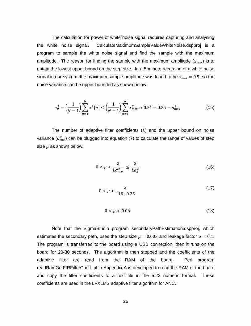
The calculation for power of white noise signal requires capturing and analysing
the white noise signal. CalculateMaximumSampleValueWhiteNoise.dspproj is a
program to sample the white noise signal and find the sample with the maximum
amplitude. The reason for finding the sample with the maximum amplitude (𝑥max) is to
obtain the lowest upper bound on the step size. In a 5-minute recording of a white noise
signal in our system, the maximum sample amplitude was found to be 𝑥max = 0.5, so the
noise variance can be upper-bounded as shown below.
𝜎𝑥2 = (
1
𝑁 − 1) ∑ 𝑥2[𝑛]
𝑁
𝑛=1
≤ (1
𝑁 − 1) ∑ 𝑥max
2
𝑁
𝑛=1
≈ 0.52 = 0.25 = 𝜎max2 (15)
The number of adaptive filter coefficients (𝐿) and the upper bound on noise
variance (𝜎max2 ) can be plugged into equation (7) to calculate the range of values of step
size 𝜇 as shown below.
0 < 𝜇 <2
𝐿𝜎max2
≤ 2
𝐿𝜎𝑥2 (16)
0 < 𝜇 <2
119 ∙ 0.25
(17)
0 < 𝜇 < 0.06 (18)
Note that the SigmaStudio program secondaryPathEstimation.dspproj, which
estimates the secondary path, uses the step size 𝜇 = 0.005 and leakage factor 𝛼 = 0.1.
The program is transferred to the board using a USB connection, then it runs on the
board for 20-30 seconds. The algorithm is then stopped and the coefficients of the
adaptive filter are read from the RAM of the board. Perl program
readRamGetFIRFilterCoeff .pl in Appendix A is developed to read the RAM of the board
and copy the filter coefficients to a text file in the 5.23 numeric format. These
coefficients are used in the LFXLMS adaptive filter algorithm for ANC.
27
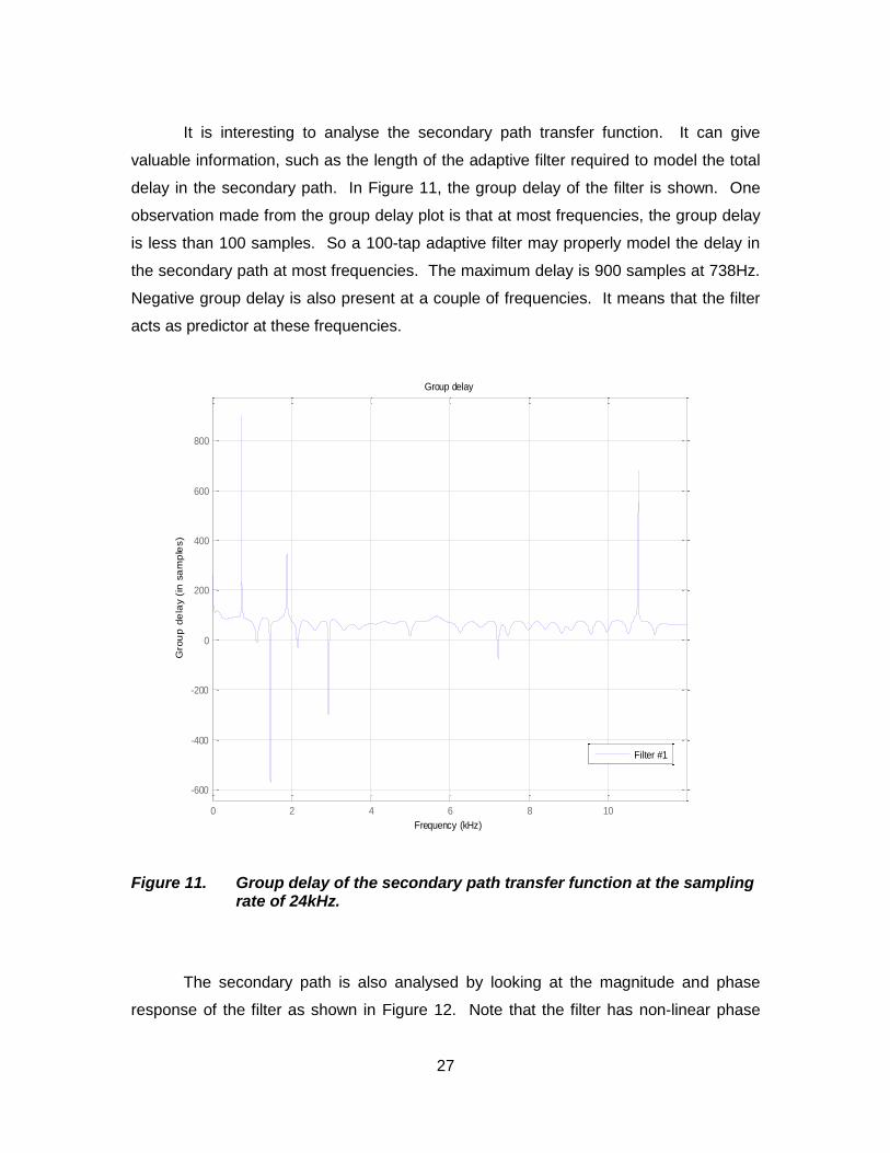
It is interesting to analyse the secondary path transfer function. It can give
valuable information, such as the length of the adaptive filter required to model the total
delay in the secondary path. In Figure 11, the group delay of the filter is shown. One
observation made from the group delay plot is that at most frequencies, the group delay
is less than 100 samples. So a 100-tap adaptive filter may properly model the delay in
the secondary path at most frequencies. The maximum delay is 900 samples at 738Hz.
Negative group delay is also present at a couple of frequencies. It means that the filter
acts as predictor at these frequencies.
Figure 11. Group delay of the secondary path transfer function at the sampling rate of 24kHz.
The secondary path is also analysed by looking at the magnitude and phase
response of the filter as shown in Figure 12. Note that the filter has non-linear phase
0 2 4 6 8 10
-600
-400
-200
0
200
400
600
800
Frequency (kHz)
Gro
up
de
lay (
in s
am
ple
s)
Group delay
Filter #1

28
response and acts approximately as a band-pass filter for frequencies around 300Hz.
Outside of the main lobe around 300Hz, the signal is attenuated by at least 7 dB.
Figure 12. Magnitude and phase plot of secondary path transfer function at the sampling rate of 24kHz.
4.2. Leaky FXLMS Adaptive Filter
LFXLMS adaptive filter is implemented in both feed forward and feedback
configuration on the ADAU1446 evaluation board. All the programming for ADAU1446 is
done using SigmaStudio software. The adaptive filter is designed using simple delay,
multiplication, addition, subtraction and feedback blocks. The available FIR filter block in
SigmaStudio is used to implement the secondary path adjustment using the coefficients
calculated as described in Section 4.1.
0 2 4 6 8 10
-50
-45
-40
-35
-30
-25
-20
-15
-10
-5
0
Frequency (kHz)
Mag
nitud
e (
dB
)
Magnitude Response (dB) and Phase Response
-214.5728
-193.9888
-173.4048
-152.8208
-132.2368
-111.6528
-91.0688
-70.4848
-49.9008
-29.3168
-8.7328
Pha
se
(ra
dia
ns)
Filter #1: Magnitude
Filter #1: Phase

29
The file demoFeedforwardLeakyFxLMS107taps.dspproj implements a feed
forward ANC configuration, while demoFeedbackLeakyFxLMS104taps.dspproj
implements a feedback ANC configuration. These files can be found in the
SigmastudioPrograms folder on the submitted CD. The software implementations are
based on the material provided in Section 2.

30
5. Test Bed
The test bed is set up to measure the performance of ANC in feed forward and
feedback configurations using the ADAU1446 DSP board. The test bed isolates the
ANC system from the outside sound interference. Also, it helps in fixing the position of
the noise speaker, error cancelling speaker and error microphone. Hence, it provides
standardised and repeatable test results.
The test bed was built within a wooden duct made from the regular plywood. The
duct has a square cross section with approximate dimension of 9 cm. The length of the
duct is 4 feet (= 121.9 cm). Vinyl wallpaper is pasted on the inside of the wooden duct,
so as to reduce reverberations produced by the rough surface of the wood. The actual
shape is shown in the figures below. Note that the physical location of speakers and
microphones does not matter as long as secondary path is measured accurately.
Figure 13. Wood-frame ANC test bed
Noise Canceling Speaker

31
Figure 14. Inside view of the wooden duct.
Noise Canceling Speaker
Error Mic
Reference Mic
Noise Source

32
6. Procedure for testing
The testing procedure is divided in two sections. The First section is the initial
test setup procedure, which will help in explaining the initial set up of the board and
making sure that everything is working as expected. It will also help the reader
understand how to use a laptop computer to capture the sound signal from the
ADAU1446 evaluation board. The second section is the actual testing of different ANC
algorithms.
6.1. Initial test setup procedure
1) Do not power on the ADAU1446 evaluation board and make sure that all the pin
connections are set to default as explained in Appendix C.
2) Do not power on SSM2167 and make sure that it has the default setting for noise
gate at 40dB and compression ratio at 1:1.
3) Make all the hardware connections as shown in Figure 9. Power on the
ADAU1446 evaluation board and power amplifier. Connect the USBi cable from
the ADAU1446 evaluation board to the laptop. Set up the USB connection as
shown in Appendix C.
4) Download a sine wave basic test (basicSineToneTest.dspproj4) to the ADAU1446
evaluation board and make sure that the sine wave is heard at the noise
generating speaker connected to the output number 0 on the board. Inside the
program, change output number to 1 and make sure the sine wave is audible at
4 This is SigmaStudio software program in SigmastudioPrograms folder on the submitted CD.

33
the error cancelling speaker. If everything works, then reset the board by
pressing the reset button.
5) Change the basicSineToneTest.dspproj program and redirect the output of the
sine wave to output number 3. Connect jack J5 from the board to the laptop
microphone input using a 3.5 audio jack cable. Start basicSineToneTest.dspproj
program on the board by using the 'download' button in the SigmaStudio
software. On the laptop, start the sound recorder application. Click on 'start
recording' and after a few seconds click on 'stop recording.' Save this file on the
laptop as sineTone500Hz.wma. Note that Windows sound recorder will always
save the file in the WMA file format.
6) Convert sineTone.wma to sineTone.wav format, so that it can be plotted in
MATLAB. To accomplish the conversion, one can use the ffmpeg utility. To set
up ffmpeg on the laptop, follow the instructions in Appendix D.
7) To plot the WAV file in time domain, frequency domain, as well as its power
spectrum, use readAndDisplayWavFile.m MATLAB program. See Appendix B
for details.
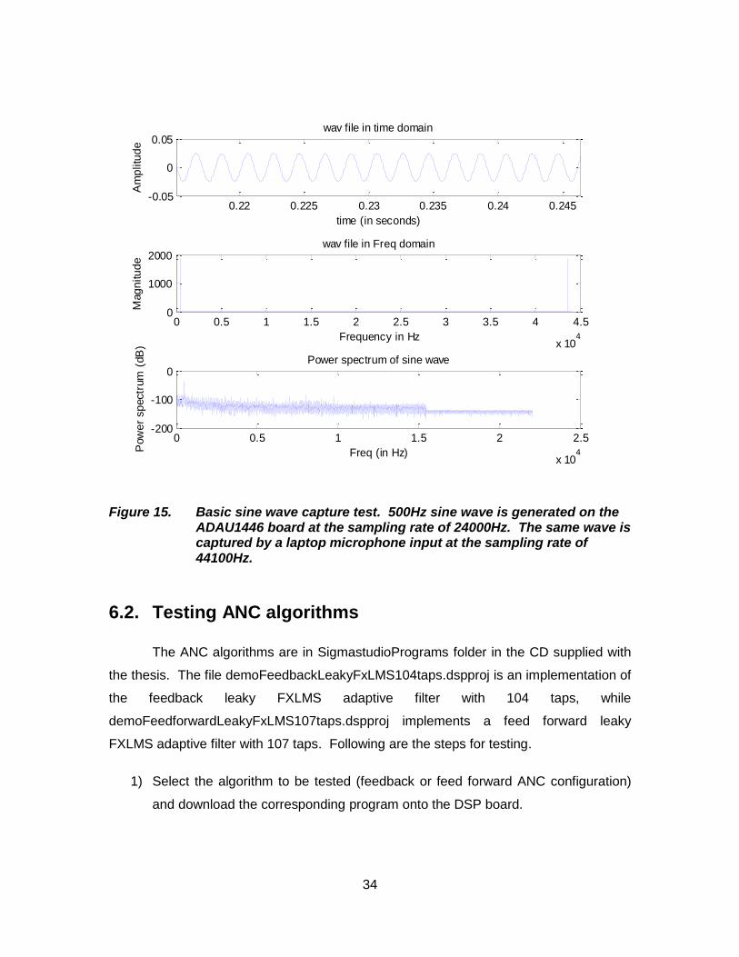
In the MATLAB plot, make sure the sine wave is not clipped. If it is clipped, decrease
the amplitude of the sine wave using volume control in basicSineToneTest.dspproj. The
preamp gain of the laptop used in the experiments was calculated as 12dB, so the
volume control in basicSineToneTest.dspproj was set at 12dB or less. For a 500Hz
sine wave from the board, the MATLAB plot is shown in the Figure 15 below. Note that
the frequency of the sine wave is easily seen from the frequency plot. The spikes are at
500Hz and 44100500 = 43600Hz in the frequency domain, where 44100Hz = 44.1kHz
is the sampling frequency. Also, the largest spike in the power spectrum is at 500Hz.
To see the WAV file captured in our tests and the corresponding MATLAB figures,
please see the resultBasicSineToneTest folder in the submitted CD.
34
Figure 15. Basic sine wave capture test. 500Hz sine wave is generated on the ADAU1446 board at the sampling rate of 24000Hz. The same wave is captured by a laptop microphone input at the sampling rate of 44100Hz.
6.2. Testing ANC algorithms
The ANC algorithms are in SigmastudioPrograms folder in the CD supplied with
the thesis. The file demoFeedbackLeakyFxLMS104taps.dspproj is an implementation of
the feedback leaky FXLMS adaptive filter with 104 taps, while
demoFeedforwardLeakyFxLMS107taps.dspproj implements a feed forward leaky
FXLMS adaptive filter with 107 taps. Following are the steps for testing.
1) Select the algorithm to be tested (feedback or feed forward ANC configuration)
and download the corresponding program onto the DSP board.
0.22 0.225 0.23 0.235 0.24 0.245-0.05
0
0.05wav file in time domain
Am
plitu
de
time (in seconds)
0 0.5 1 1.5 2 2.5 3 3.5 4 4.5
x 104
0
1000
2000wav file in Freq domain
Frequency in Hz
Mag
nitu
de
0 0.5 1 1.5 2 2.5
x 104
-200
-100
0Power spectrum of sine wave
Pow
er
sp
ectr
um
(dB
)
Freq (in Hz)

35
2) Make sure all the steps in Section 6.1 are completed and the output number 3
from the DSP board is connected to the laptop via the 3.5 audio jack cable.
3) Both ANC programs (feed forward and feedback) have a switch that can turn the
adaptive algorithm ON and OFF. Make sure the switch is at the OFF position.
4) On the laptop, open the sound recorder application and start recording. This will
start capturing the signal at output number 3 of the board, which is the error
signal. Since the adaptive algorithm is turned OFF, the error signal will be a pure
sine wave. After a few seconds, stop the recording and save the file as
<InputSignalFreq>.wav. Now, turn on the adaptive algorithm by moving the
software switch to the ON position. Again, start recording the signal from the
output number 3 of the board. After a few seconds stop the recording. Save this
recorded file as <InputSignalFreq>_ANC.wav.
5) Use ffmpeg to convert the recorded files from WMA format to WAV format. Note
that ffmpeg instructions are provided in Appendix D.
6) Plot the power spectrum of both signals in the WAV files using
comparePSDAudioWav.m MATLAB program in Appendix B.
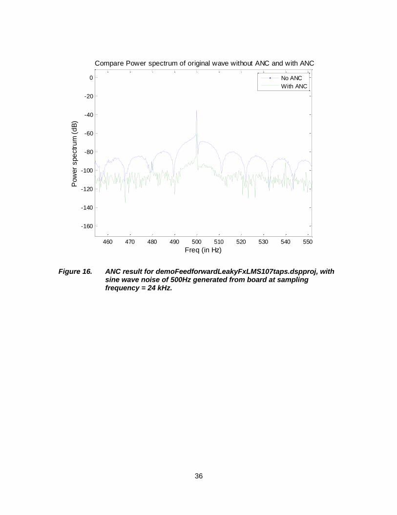
7) Analyse the power plot. If the ANC algorithm was successful in cancelling the
noise, then the power spectrum curve of the signal with ANC will be below the
corresponding curve of the signal without ANC, as shown in Figure 16 below.
36
Figure 16. ANC result for demoFeedforwardLeakyFxLMS107taps.dspproj, with sine wave noise of 500Hz generated from board at sampling frequency = 24 kHz.
460 470 480 490 500 510 520 530 540 550
-160
-140
-120
-100
-80
-60
-40
-20
0
Freq (in Hz)
Pow
er
spe
ctr
um
(d
B)
Compare Power spectrum of original wave without ANC and with ANC
No ANC
With ANC

37
7. Results and Discussion
The ANC performance using feed forward LFXLMS and feedback LFXLMS was
examined across a range of frequencies. The results of feed forward LFXLMS are
discussed in Section 7.1, while those of feedback LFXLMS are discussed in Section 7.2.
Note that 24 kHz is the sampling rate of the ADAU1446 board and should not be
confused with 44.1 kHz, which is the sampling rate of the sound recorder on the laptop.
7.1. Result of ANC by feed forward LFXLMS
Sound cancellation performance is examined at different frequencies from 150Hz
to 8000Hz. This range is chosen because human ear is most sensitive to frequencies
from 1000Hz - 5000Hz (Gelfand, 1990). Also the upper bound of frequency range
8000Hz is less than the maximum frequency measured (i.e. 12000Hz) by the ADAU1446
board with sampling rate of 24000 Hz. Some of the comparisons of the power spectra
with and without ANC are shown in Figure 17 to Figure 22 below. The complete
comparison results for all the frequencies are in the resultMatlabPlot folder in the
supplied CD.

38
Figure 17. Comparison of power spectra with and without ANC at 800Hz
Figure 18. Comparison of power spectra with and without ANC at 800Hz. The graph is magnified around 800Hz.
0 0.5 1 1.5 2 2.5
x 104
-200
-180
-160
-140
-120
-100
-80
-60
-40
-20
Freq (in Hz)
Pow
er
spe
ctr
um
(d
B)
Compare Power spectrum of original wave without ANC and with ANC
No ANC
With ANC
650 700 750 800 850 900 950
-160
-140
-120
-100
-80
-60
-40
-20
0
Freq (in Hz)
Pow
er
spe
ctr
um
(d
B)
Compare Power spectrum of original wave without ANC and with ANC
No ANC
With ANC

39
Figure 19. Comparison of power spectra with and without ANC at 7000Hz
Figure 20. Comparison of power spectra with and without ANC at 7000Hz. The graph is magnified around 7000Hz.
0 0.5 1 1.5 2 2.5
x 104
-200
-180
-160
-140
-120
-100
-80
-60
-40
-20
Freq (in Hz)
Pow
er
spe
ctr
um
(d
B)
Compare Power spectrum of original wave without ANC and with ANC
No ANC
With ANC
6960 6970 6980 6990 7000 7010 7020 7030 7040 7050
-160
-140
-120
-100
-80
-60
-40
-20
0
Freq (in Hz)
Pow
er
spe
ctr
um
(d
B)
Compare Power spectrum of original wave without ANC and with ANC
No ANC
With ANC

40
Figure 21. Comparison of power spectra with and without ANC at 3000Hz
Figure 22. Comparison of power spectra with and without ANC at 3000Hz. The graph is magnified around 3000Hz.
0 0.5 1 1.5 2 2.5
x 104
-180
-160
-140
-120
-100
-80
-60
-40
-20
Freq (in Hz)
Pow
er
spe
ctr
um
(d
B)
Compare Power spectrum of original wave without ANC and with ANC
No ANC
With ANC
2980 2985 2990 2995 3000 3005 3010 3015 3020-140
-120
-100
-80
-60
-40
-20
0
Freq (in Hz)
Pow
er
spe
ctr
um
(d
B)
Compare Power spectrum of original wave without ANC and with ANC
No ANC
With ANC
41
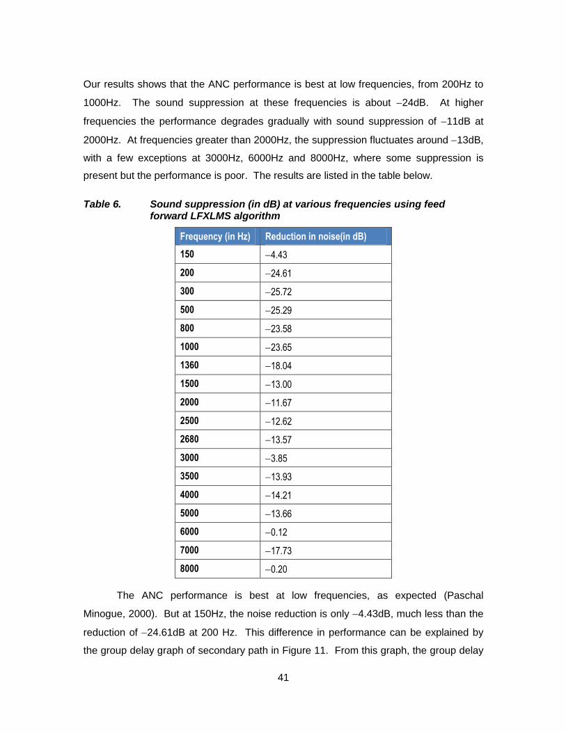
Our results shows that the ANC performance is best at low frequencies, from 200Hz to
1000Hz. The sound suppression at these frequencies is about 24dB. At higher
frequencies the performance degrades gradually with sound suppression of 11dB at
2000Hz. At frequencies greater than 2000Hz, the suppression fluctuates around 13dB,
with a few exceptions at 3000Hz, 6000Hz and 8000Hz, where some suppression is
present but the performance is poor. The results are listed in the table below.
Table 6. Sound suppression (in dB) at various frequencies using feed forward LFXLMS algorithm
Frequency (in Hz) Reduction in noise(in dB)
150 4.43
200 24.61
300 25.72
500 25.29
800 23.58
1000 23.65
1360 18.04
1500 13.00
2000 11.67
2500 12.62
2680 13.57
3000 3.85
3500 13.93
4000 14.21
5000 13.66
6000 0.12
7000 17.73
8000 0.20
The ANC performance is best at low frequencies, as expected (Paschal
Minogue, 2000). But at 150Hz, the noise reduction is only 4.43dB, much less than the
reduction of 24.61dB at 200 Hz. This difference in performance can be explained by
the group delay graph of secondary path in Figure 11. From this graph, the group delay

42
is very large at frequencies below 200 Hz, so a larger number of taps is required in the
adaptive filter to model the delay in the secondary path. The group delay at 150 Hz is
approximately 130 samples. The adaptive filter in the current implementation has only
107 taps, which could be the reason for the poor performance at 150 Hz.
The performance at 3000 Hz, 6000 Hz and 8000 Hz is also poor compared to
other high frequencies. The group delay at these frequencies is approximately 80, 70
and 45, respectively. Since these group delays are less than the number of taps of the
adaptive filter (107), the group delay does not explain the poor performance of the
system at these frequencies. A more likely explanation for the poor performance is that
the estimation of the secondary path transfer function at these frequencies is less
accurate. This estimation can be made better by increasing the size of adaptive filter
and the time interval used for secondary path estimation.
The noise reduction (in dB) vs. frequency of the noise signal (in Hz) from Table 6
is shown as blue circles in Figure 23 below. The red line joining the blue dots shows the
overall trend of noise reduction.
Figure 23. Noise reduction vs. frequency for ANC using feed forward adaptive filter. Red line shows the overall trend of noise reduction.
0 1000 2000 3000 4000 5000 6000 7000 8000-30
-25
-20
-15
-10
-5
0
Freq(in Hz)
Noi
se R
edu
ctio
n(in
dB
)

43
The feed forward adaptive algorithm is also tested on a broadband signal (white
noise). The plot of power spectra shows that the noise power spectrum without ANC
(blue line) is above the noise power spectrum with ANC (green line). Although the
reduction is in the range 5-10 dB, the graph indicates that suppression is possible even
for broadband signals.
Figure 24. Compare white noise power spectrum with ANC and without ANC for feed forward adaptive filter.
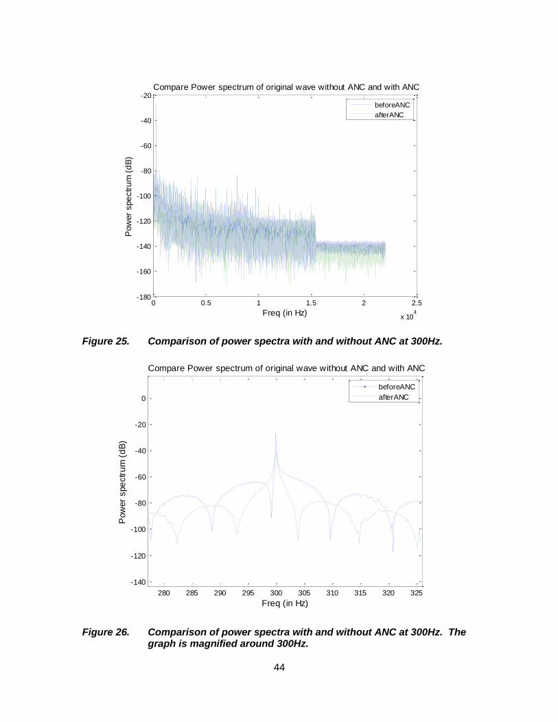
7.2. Results of ANC by feedback LFXLMS
As in the feed forward case, the performance of the feedback ANC system is
measured across a range of frequencies from 150Hz to 8000Hz. All the results are
provided in the resultMatlabPlot folder in supplied CD. Some representative plots of the
power spectra are shown in Figure 25 to Figure 30 below. The Magnified results near
the operating frequency are also provided for clearer comparison.
0 0.5 1 1.5 2 2.5
x 104
-180
-160
-140
-120
-100
-80
-60
-40
Freq (in Hz)
Pow
er
spe
ctr
um
(d
B)
Compare Power spectrum of original wave without ANC and with ANC
No ANC
With ANC
44
Figure 25. Comparison of power spectra with and without ANC at 300Hz.
Figure 26. Comparison of power spectra with and without ANC at 300Hz. The graph is magnified around 300Hz.
0 0.5 1 1.5 2 2.5
x 104
-180
-160
-140
-120
-100
-80
-60
-40
-20
Freq (in Hz)
Pow
er
spe
ctr
um
(d
B)
Compare Power spectrum of original wave without ANC and with ANC
beforeANC
afterANC
280 285 290 295 300 305 310 315 320 325
-140
-120
-100
-80
-60
-40
-20
0
Freq (in Hz)
Pow
er
spe
ctr
um
(d
B)
Compare Power spectrum of original wave without ANC and with ANC
beforeANC
afterANC

45
Figure 27. Comparison of power spectra with and without ANC at 500Hz
Figure 28. Comparison of power spectra with and without ANC at 500Hz. The graph is magnified around 500Hz.
0 0.5 1 1.5 2 2.5
x 104
-200
-180
-160
-140
-120
-100
-80
-60
-40
-20
Freq (in Hz)
Pow
er
spe
ctr
um
(d
B)
Compare Power spectrum of original wave without ANC and with ANC
beforeANC
afterANC
475 480 485 490 495 500 505 510 515 520
-140
-120
-100
-80
-60
-40
-20
0
20
Freq (in Hz)
Pow
er
spe
ctr
um
(d
B)
Compare Power spectrum of original wave without ANC and with ANC
beforeANC
afterANC

46
Figure 29. Comparison of power spectra with and without ANC at 5000Hz.
Figure 30. Comparison of power spectra with and without ANC at 5000Hz. The graph is magnified around 5000Hz.
0 0.5 1 1.5 2 2.5
x 104
-180
-160
-140
-120
-100
-80
-60
-40
-20
Freq (in Hz)
Pow
er
spe
ctr
um
(d
B)
Compare Power spectrum of original wave without ANC and with ANC
beforeANC
afterANC
4975 4980 4985 4990 4995 5000 5005 5010 5015 5020-140
-120
-100
-80
-60
-40
-20
0
Freq (in Hz)
Pow
er
spe
ctr
um
(d
B)
Compare Power spectrum of original wave without ANC and with ANC
beforeANC
afterANC
47
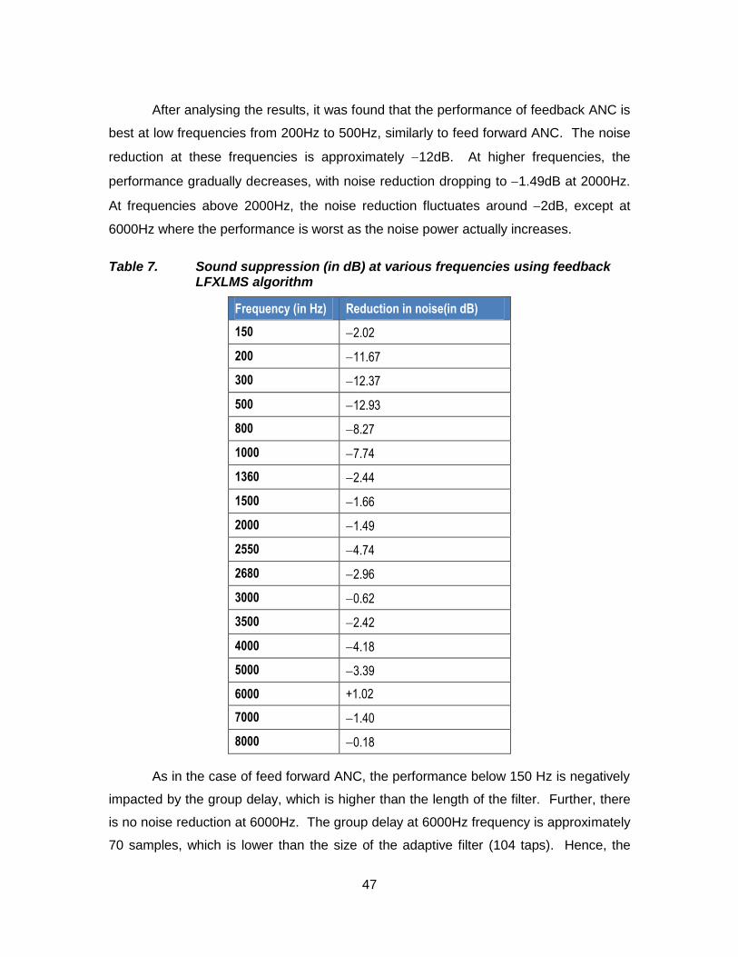
After analysing the results, it was found that the performance of feedback ANC is
best at low frequencies from 200Hz to 500Hz, similarly to feed forward ANC. The noise
reduction at these frequencies is approximately 12dB. At higher frequencies, the
performance gradually decreases, with noise reduction dropping to 1.49dB at 2000Hz.
At frequencies above 2000Hz, the noise reduction fluctuates around 2dB, except at
6000Hz where the performance is worst as the noise power actually increases.
Table 7. Sound suppression (in dB) at various frequencies using feedback LFXLMS algorithm
Frequency (in Hz) Reduction in noise(in dB)
150 2.02
200 11.67
300 12.37
500 12.93
800 8.27
1000 7.74
1360 2.44
1500 1.66
2000 1.49
2550 4.74
2680 2.96
3000 0.62
3500 2.42
4000 4.18
5000 3.39
6000 +1.02
7000 1.40
8000 0.18
As in the case of feed forward ANC, the performance below 150 Hz is negatively
impacted by the group delay, which is higher than the length of the filter. Further, there
is no noise reduction at 6000Hz. The group delay at 6000Hz frequency is approximately
70 samples, which is lower than the size of the adaptive filter (104 taps). Hence, the

48
group delay does not explain the poor performance of system at this frequency. The
suspected reason for such performance is the inaccuracy of the estimate of the
secondary path transfer function at high frequencies. This estimate can possibly be
improved by increasing the size of the adaptive filter employed in secondary path
estimation.
The noise reduction (in dB) vs. frequency of the noise signal (in Hz) from Table 7
is shown as blue circles in Figure 31 below. The red line joining the blue dots shows the
overall trend of noise reduction.
Figure 31. Plot noise reduction verses frequency for feedback adaptive filter. Red line shows the overall trend of noise reduction.
The feedback algorithm is also tested in the context of broadband noise cancellation
using white noise. As shown in Figure 32 below, the feedback configuration is also able
to cancel noise, although by lower amount than the feed forward configuration.
0 1000 2000 3000 4000 5000 6000 7000 8000-14
-12
-10
-8
-6
-4
-2
0
2
Freq(in Hz)
Nois
e R
ed
uctio
n(i
n d
B)

49
Figure 32. Comparison of white noise power spectra with and without ANC using feedback adaptive filter.
By comparing the performance of feed forward LFXLMS and feedback LFXLMS
algorithm, it is clear that the performance of feed forward LFXLMS is better than that of
the feedback LFXLMS, even though both the algorithms employ adaptive filters of
approximately the same size. This is due to the fact that in the current implementation,
fewer estimates are used in the feed forward configuration compared to the feedback
configuration. For example, the exact noise signal is provided as reference noise signal
to the feed forward LFXLMS algorithm internally from the board, whereas in the
feedback LFXLMS algorithm, the reference noise signal is estimated from the error
signal and the output of the adaptive filter. One way to improve the performance of the
feedback algorithm is by increasing the estimation accuracy of the reference noise
signal. This accuracy can be improved by increasing the size of the adaptive filter used
to estimate secondary path.
0 1000 2000 3000 4000 5000 6000
-130
-120
-110
-100
-90
-80
-70
-60
-50
Freq (in Hz)
Pow
er
spe
ctr
um
(d
B)
Compare Power spectrum of original wave without ANC and with ANC
No ANC
With ANC

50
8. Conclusions
In this thesis, an ANC test bed was developed around the ADAU1446-Eval audio
processing board. Single-channel ANC system was implemented using two different
adaptive filter approaches - feed forward LFXLMS and feedback LFXLMS. Both ANC
systems were able to successfully cancel narrowband and broadband noise, especially
at low frequencies. The feed forward system was found to be better than the feedback
system in cancelling the unwanted signal, because fewer estimates were involved.

51
9. Future Improvements
i. The adaptive filter design may be improved by changing the LMS adaptive
algorithm to NLMS (Normalised LMS) adaptive algorithm in the ANC system
(Alok Pandey, 2012). In the NLMS adaptive filter, step size is independent of
signal power. The step size will depend upon the number of taps of the adaptive
filter (𝐿) and the number of samples corresponding to the overall delay in the
secondary path (∆). The step size can easily be found from equation (19) below.
This will make the design of ANC system independent of the power of the input
signal.
0 < 𝜇 <2
(𝐿 + ∆) (19)
ii. A reduction in complexity may be achieved by implementing the adaptive filter
algorithm in the frequency domain instead of time domain. One of the effective
frequency-domain algorithms is Fast LMS. It is based on block processing using
FFT (Fast Fourier Transform), and requires less computation. Hence, adaptive
filters of large size can be realized. According to (National Instruments, 2009), if
both the filter length and the block size are 𝑁, the standard LMS algorithm
requires 𝑁(2𝑁 + 1) multiplications, whereas the fast block LMS algorithm
requires only 10𝑁log2𝑁 + 26𝑁 multiplications. For example, with 𝑁 = 1024, the
fast block LMS algorithm requires 16 times fewer multiplications than the
standard LMS algorithm.
iii. The DSP processor ADAU1446 does not support FFT operations, so to
implement Fast LMS, a new DSP processor with high clock speed and high
number of MMACs (Million Multiply Accumulate Cycles per second) is required.
High clock speed will insure more instruction per second at a given sampling

52
rate. The performance of filtering and FFT depends upon the number of MMACs
in the system. In order to realize noise cancellation in 3D space, DSP chip
should also have synchronous multiple audio input and output interfaces (i.e. I2S
interfaces). If the DSP chip supports master-slave mode, then all these chips
can be cascaded to increase the ability of the system to cancel noise in large
volumes.
iv. The ANC design can be improved if enabling and disabling down sampling and
up sampling on the DSP chip can be achieved in software. It will make the
design of the adaptive filter more flexible. For example, if the DSP core is
running at 172 MHz clock, then 48 kHz sampling rate will only give 3583
instructions per second. On the other hand, consider the situation in which the
maximum noise frequency to be cancelled is 4 kHz, then the required minimum
sampling rate of the DSP board is 8 kHz. This will increase the required number
of instructions per second to 3583 ∙ 6 = 21,498.
v. The ANC system in all the implementations above uses traditional audio signal
chain as shown in Figure 8. For future development, it is worth considering a
fully digital audio signal chain as shown in Figure 33 below.
DSP Board
Microphone Power Amplifier Speaker
Digital Signals
1010101 10101011010101
Figure 33. Fully digital audio signal chain (adapted from (Lewis J. , Common Inter IC digital interface for audio data transfer))
Digital audio signal chain implementation is cheaper, as it require less hardware;
for example, no preamp is required. Since the signal chain is digital, the
secondary path can be measured more accurately with an adaptive filter of
smaller size, which might improve the performance of the ANC system.
vi. Implementation of feed forward adaptive filter approach with reference
microphone and no error microphone. This approach will be similar to the

53
feedback configuration, except that the error signal will be estimated from the
reference noise signal. This algorithm will require offline modelling of the
acoustic path 𝐸(𝑧) from the reference microphone to the error microphone.
Once this transfer function is known, error signal can be calculated as shown in
Figure 34 below.
W(z)Weights of FIR
filter
Leaky LMSS^(z)
Estimation of secondary path
Reference Mic
Noise Cancelling Speaker
x'(n)
x(n)
- y(n)
LFXLMS Adaptive Algorithm
Adaptive Filter
E(z), Estimation of acoustic path from
reference mic to summing junction
e(n)
+
+
Noise Source
Noise Signal
=
d(n)
- y(n)
+Residual Noise
Figure 34. Feed forward adaptive filter approach with no error microphone

54
References
Alok Pandey, L. M. (2012). Comparative Study of LMS and NLMS Algorithms in Adaptive Equalizer. International Journal of Engineering Research and Applications (IJERA).
Analog Devices. (2013). ADAU1446 datasheet. Retrieved 08 22, 2013, from http://www.analog.com/en/audiovideo-products/audio-signal-processors/adau1446/products/product.html
Analog Devices. (2013). Datasheet of ADMP504. Retrieved from http://www.analog.com/en/audiovideo-products/mems-microphones/admp504/products/product.html
Analog Devices. (2013). Datasheet SSM2167. Retrieved 08 23, 2013, from http://www.analog.com/en/audiovideo-products/audio-signal-processors/ssm2167/products/product.html
Analog Devices. (n.d.). Sigma studio software. Retrieved from http://www.analog.com/en/content/cu_over_sigmastudio_graphical_dev_tool_overview/fca.html
Analog devices wiki. (2013, 08 01). Retrieved 08 22, 2013, from http://wiki.analog.com/resources/tools-software/sigmastudio/usingsigmastudio/numericformats
Gelfand, S. A. (1990). Hearing: An introduction to psychological and physiological acoustics. New York and Basel: Marcel Dekker, Inc.
Haykin, S. (2002). Adaptive Filter Theory. Prentice Hall.
Lewis, J. (2012). Understanding Microphone Sensitivity. Retrieved 08 23, 2013, from http://www.analog.com/library/analogdialogue/archives/46-05/understanding_microphone_sensitivity.html
Lewis, J. (n.d.). Common Inter IC digital interface for audio data transfer. Technical Article, Analog devices.
National Instruments. (2009). LMS algorithms. Retrieved from http://zone.ni.com/reference/en-XX/help/372357A-01/lvaftconcepts/aft_lms_algorithms/

55
Paschal Minogue, N. R. (2000). Adaptively Cancelling Server Fan Noise: Principles and Experiments with a Short Duct and the AD73522 dspConverter. Analog Dialogue 34-2 (2000).
Sayed, A. H. (2008). Adaptive filters. John Wiley & Sons. Retrieved 08 21, 2013, from http://zone.ni.com/reference/en-XX/help/372357A-01/lvaftconcepts/aft_lms_algorithms/
Sen M Kuo, B. H. (2001). Real time digital signal processing. John wiley and son ltd.
Sen M. Kuo, D. R. (1999). Active Noise Control: A Tutorial Review. Proceedings Of The IEEE.
Texas Instuments. (2012, July). 15-W FILTER-FREE STEREO CLASS-D AUDIO POWER AMPLIFIER With SPEAKERGUARD . Retrieved from TI: http://www.ti.com/lit/ds/slos528d/slos528d.pdf
V. John Mathews, S. C. (2003). Adaptive Filters.
Visaton. (2013, Jul). FRS 5 - 8 Ohm. Retrieved from Visaton: http://www.visaton.com/en/chassis_zubehoer/breitband/frs5_8.html
Wikibooks. (2012). Engineering Acoustics/Sound Absorbing Structures and Materials. Retrieved from Wikibooks: http://en.wikibooks.org/wiki/Engineering_Acoustics/Sound_Absorbing_Structures_and_Materials

56
Appendices

57
Appendix A. Perl programs
readRamGetFIRFilterCoeff .pl
Perl program (readRamGetFIRFilterCoeff .pl) to read ram file of ADAU1446 evaluation board and copy coefficients of FIR filter to text file in 5.23 format. This text file will be used by Leaky FXLMS adaptive algorithm. Cygwin command to run this program is ‘perl readRamGetFIRFilterCoeff .pl’
#### Written by S Sidhu, SFU###############
use strict;
use warnings;
my $InFileName = 'ram.txt';
my $OutFileName = 'FirFiltCoeffAtSamplingRate24k.txt';
open(my $InFD, '<', $InFileName)
or die "ERROR: Could not open file '$InFileName' $!";
my @InLines;
while (<$InFD>)
$_ =~ s/^\s+|\s+$//g;
push(@InLines, $_);
my @OutLines;
for (my $ii = 0; $ii <= $#InLines; $ii++)
if($InLines[$ii] =~ m/ReadBackAlgSigma/)
if($InLines[$ii+4] eq "Data 5.32:") #add more checks
print "match found at ii+5 = $ii+5\n";
push(@OutLines, $InLines[$ii+5]);
else
die "ERROR: match not found at ii+5 = $ii+5\n";
open(my $OutFD, '>', $OutFileName)
or die "ERROR: Could not open file '$OutFileName' $!";
for (my $ii = 0; $ii <= $#OutLines; $ii++)
print $OutFD "$OutLines[$ii]\n";
close $InFD;
close $OutFD;

58
Appendix B. MATLAB programs
readAndDisplayWavFile.m
MATLAB program (readAndDisplayWavFile.m) to read WAV file and plot it in time domain, frequency domain and power spectrum.
%#### written by S Sidhu, SFU#########
inputfile = 'sineTone500Hz.wav';
%read wav file to array
[wave,fs]=wavread(inputfile);
%plot in time domain
t=0:1/fs:(length(wave)-1)/fs;
figure('name', inputfile);
subplot(3,1,1); plot(t,wave);
title('wav file in time domain');
ylabel('Amplitude');
xlabel('time (in seconds)');
%plot in freq domain
n=length(wave)-1;
f=0:fs/n:fs;
wavefft=abs(fft(wave));
subplot(3,1,2); plot(f,wavefft);
title('wav file in Freq domain');
xlabel('Frequency in Hz');
ylabel('Magnitude');
%plot power
[P,F] = periodogram(wave,[],length(wave),fs,'power');
subplot(3,1,3); plot(F,10*log10(P));
title('Power spectrum of sine wave');
ylabel('Power spectrum (dB)');
xlabel('Freq (in Hz)');

59
readFIRCoeffAnalyseFilterResponse.m
This program will read the coefficients of secondary path filter from text file. It will open the frequency analysis tool in MATLAB. This tool can be used to analyse the magnitude response, frequency response and group delay of filter.
%##### written by S Sidhu, SFU##########
%read FIR coeff from file
close all;
clear all;
clc;
fid = fopen('FirFiltCoeffAtSamplingRate24k.txt', 'r');
Num = textscan(fid,'%f64','delimiter','\n');
tmpB = cell2mat(Num);
B = tmpB';
% display coeff in matlab consol
disp(B);
%open fvtool, default is grpdelay
hFVT = fvtool(B,1,'Analysis','grpdelay');
set(hFVT,'Fs',44100);
legend(hFVT);
fclose(fid);
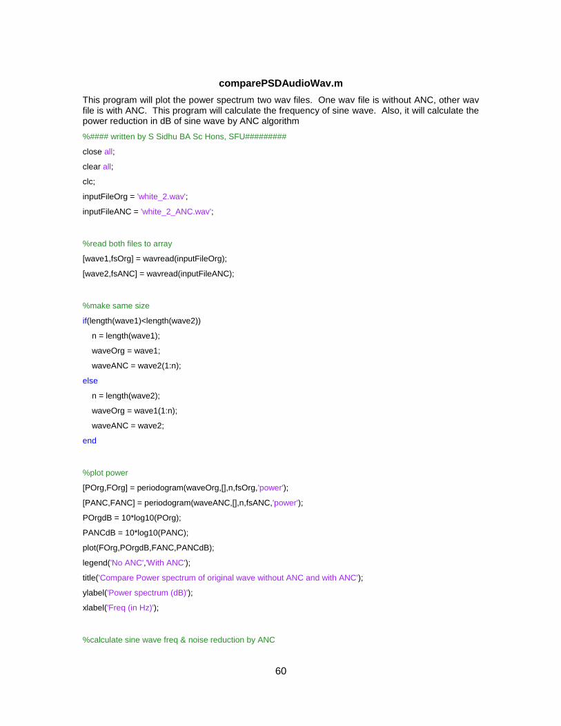
60
comparePSDAudioWav.m
This program will plot the power spectrum two wav files. One wav file is without ANC, other wav file is with ANC. This program will calculate the frequency of sine wave. Also, it will calculate the power reduction in dB of sine wave by ANC algorithm
%#### written by S Sidhu BA Sc Hons, SFU#########
close all;
clear all;
clc;
inputFileOrg = 'white_2.wav';
inputFileANC = 'white_2_ANC.wav';
%read both files to array
[wave1,fsOrg] = wavread(inputFileOrg);
[wave2,fsANC] = wavread(inputFileANC);
%make same size
if(length(wave1)<length(wave2))
n = length(wave1);
waveOrg = wave1;
waveANC = wave2(1:n);
else
n = length(wave2);
waveOrg = wave1(1:n);
waveANC = wave2;
end
%plot power
[POrg,FOrg] = periodogram(waveOrg,[],n,fsOrg,'power');
[PANC,FANC] = periodogram(waveANC,[],n,fsANC,'power');
POrgdB = 10*log10(POrg);
PANCdB = 10*log10(PANC);
plot(FOrg,POrgdB,FANC,PANCdB);
legend('No ANC','With ANC');
title('Compare Power spectrum of original wave without ANC and with ANC');
ylabel('Power spectrum (dB)');
xlabel('Freq (in Hz)');
%calculate sine wave freq & noise reduction by ANC
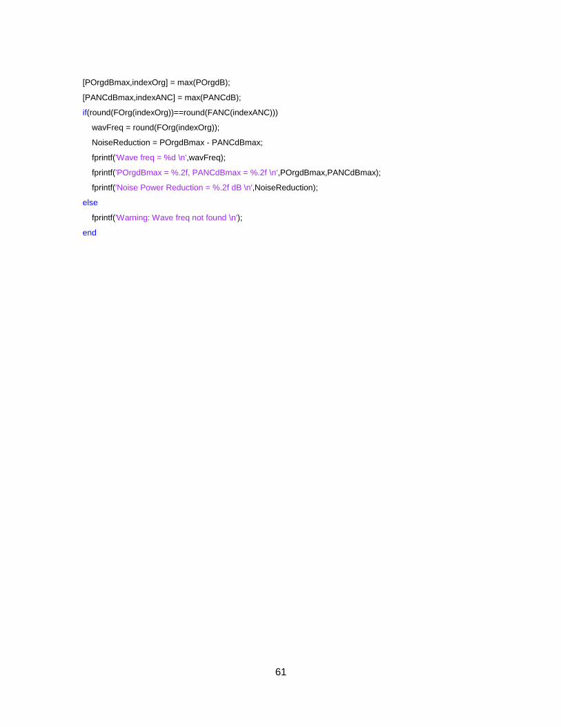
61
[POrgdBmax,indexOrg] = max(POrgdB);
[PANCdBmax,indexANC] = max(PANCdB);
if(round(FOrg(indexOrg))==round(FANC(indexANC)))
wavFreq = round(FOrg(indexOrg));
NoiseReduction = POrgdBmax - PANCdBmax;
fprintf('Wave freq = %d \n',wavFreq);
fprintf('POrgdBmax = %.2f, PANCdBmax = %.2f \n',POrgdBmax,PANCdBmax);
fprintf('Noise Power Reduction = %.2f dB \n',NoiseReduction);
else
fprintf('Warning: Wave freq not found \n');
end

62
Appendix C.
Using the Eval-ADAU144xEBZ with SigmaStudio5
SigmaStudio SOFTWARE INSTALLATION
SigmaStudio™ must be installed to use the EVAL-ADAU144xEBZ. To install the Sigma Studio software, obtain the password from the QuickStart™ Guide and follow these steps:
1. If Microsoft® .NET Framework Version 2.0 is not already installed on the PC, install it by downloading the redistri-butable package from the Microsoft website.
2. Download the SigmaStudio software from http://www.analog.com/sigmastudiodownload
3. Open the .zip file and extract the files to your PC.
4. Install SigmaStudio by double-clicking setup.exe and following the prompts. A computer restart is not required.
INSTALLING THE DRIVERS
After SigmaStudio is installed, follow these steps to install the drivers:
1. Plug the USBi into the USB port of the PC using the included mini USB cable.
2. If this is the first time the USBi has been connected to the PC, the Windows Found New Hardware notification should appear in the taskbar.
Windows Found New Hardware Notification
3. When the Found New Hardware Wizard opens, click Install from a list or specific location (Advanced).
4. Click Next.
5 This section is extracted from ADAU1446-evaluation board guide

63
Windows Found New Hardware Wizard
5. Click Search for the best driver in these locations and select Include this location in the search.
6. Click Browse and select the USB drivers subfolder, located in the SigmaStudio install directory.
7. Click Next.
Windows Found New Hardware Wizard Search and Install Options
8. When the warning about Windows logo testing appears, click Continue Anyway. Next, Windows proceeds with the installation of the drivers, as shown in Figure
Windows Logo Test Warning

64
Windows Installation of the USBi Drivers
9. When the installation of the drivers is complete, the window shown in Figure appears. Click Finish.
Driver Installation Complete
A notification of successful installation should appear in the taskbar, as shown
Successful Driver Installation Notification
CONNECTING THE EVALUATION BOARD
1. Plug the included dc power supply into the J24 power jack on the board.
2. Connect the USBi 10-pin communication cable to the J18 communications port on the evaluation board.
ADDING THE EVAL-ADAU144xEBZ TO A SigmaStudio PROJECT
To use the EVAL-ADAU144xEBZ with SigmaStudio, follow these steps:
1. Start the SigmaStudio software.
2. Begin a new project by opening the File menu and selecting New Project. (The keyboard shortcut for this operation is Ctrl + N.)
3. The default view in SigmaStudio is the Hardware Configuration tab.

65
On the left side of the screen is the Tree Toolbox tab.
Within the Tree Toolbox there is a subsection called Communication Channels. From the list of Communi-cation Channels, click and hold USBi dragging it to the right into the empty white project space.
Adding the USBi Communication Channel to the Evaluation Board for the ADAU144x
Adding a USBi to the Project
If SigmaStudio cannot detect the USBi on the USB port of the computer, the background of the USB label turns red, as shown in Figure below. This happens if the USBi is not connected or when the drivers are not installed correctly.
EVAL-ADAU144xEBZ Not Detected by SigmaStudio
If SigmaStudio detects the USBi on the USB port, the back-ground of the USB label changes to orange, as shown in Figure below
USBi Detected by SigmaStudio
ADDING AN ADAU144x IC
To communicate with the targeted ADAU144x IC on the evaluation board, add ADAU144x to the processor list in SigmaStudio.

66
Adding an ADAU144x IC
To use the USBi to communicate with the target ADAU144x IC, click the top blue pin of the USB and drag a wire to the green pin of the ADAU144x IC 1, as shown in Figure below. The I2C Address 0x70 is assigned automatically.
Connecting the EVAL-ADAU144xEBZ to an ADAU144x IC
ADDING A SELF-BOOT EEPROM
To evaluate the EVAL-ADAU144xEBZ self-boot functionality, an E2Prom IC must be added to the project. This corresponds to the EEPROM U2 device on the evaluation board.
10. Click and drag an E2Prom IC into the project space.
11. Drag a wire from the second blue pin on the USBi to the green pin on the E2Prom IC, as shown in Figure
Adding an E2Prom IC
When the second pin on the USBi communication channel is connected to the EEPROM, I2C Address 0xA0 is assigned automatically.
Connecting the EVAL-ADAU144xEBZ to the E2Prom IC
An E2Prom IC does not have to be added unless the self-boot functionality of the board is required.
PROGRAMMING THE SIGNAL FLOW
To program the signal processing flow, use the Schematic tab, located at the top of the window as shown in Figure. Click the Schematic tab.
Schematic Tab
The left side of the schematic box shows the Tree ToolBox. It contains a list of all signal processing algorithms for use in the ADAU144x, as shown in Figure below

67
Tree ToolBox
12. Open the Sources. Open oscillatory sources. Pick and drag sine wave to the schematic.
13. Open the IO. Drag output to the schematic.
14. Open Volume control. Click on the single/multiple control. Open no slew tab and drag single volume control to the schematic.
Attach all the tree components in step 12 to 14. The final schematic will be same as shown in figure below.
Basic sine wave test using sigma studio
15. Connect a pair of headphones or powered speakers to the audio output jack, J4.

68
16. Click the Link Compile Download button to download the program to the ADAU144x IC.
Link Compile Download
17. You should be hearing sine wave in the device attached to jack 4.
Default Switch and Jumper Setting Descriptions
The default setup represents the state of the board when it leaves the factory. With this configuration, the analog audio is routed from the input connectors to the codecs, in and out of the DSP, back through the codecs, and to the output connectors. Descriptions with direction references are based on the orientation of the board shown in ADAU1446-Eval board manual.
Default Switch and Jumper Setting Descriptions (Analog Devices, 2013)

69
Appendix D. FFmpeg for audio file conversion
FFmpeg is used to convert audio and video streams from one format to other. To set up ffmpeg on windows laptop the detailed instructions are at http://www.wikihow.com/Install-FFmpeg-on-Windows.
Cygwin command for converting wma file to wav file is
ffmpeg.exe -i <inputFileName.wma> -ac <numberOfChannels> <outputFileName.wav>
e.g.
ffmpeg.exe -i 2000Hz.wma -ac 1 2000Hz.wav


