
• Low Pass Filter
• High Pass Filter
• Band pass Filter
• Blurring
• Sharpening
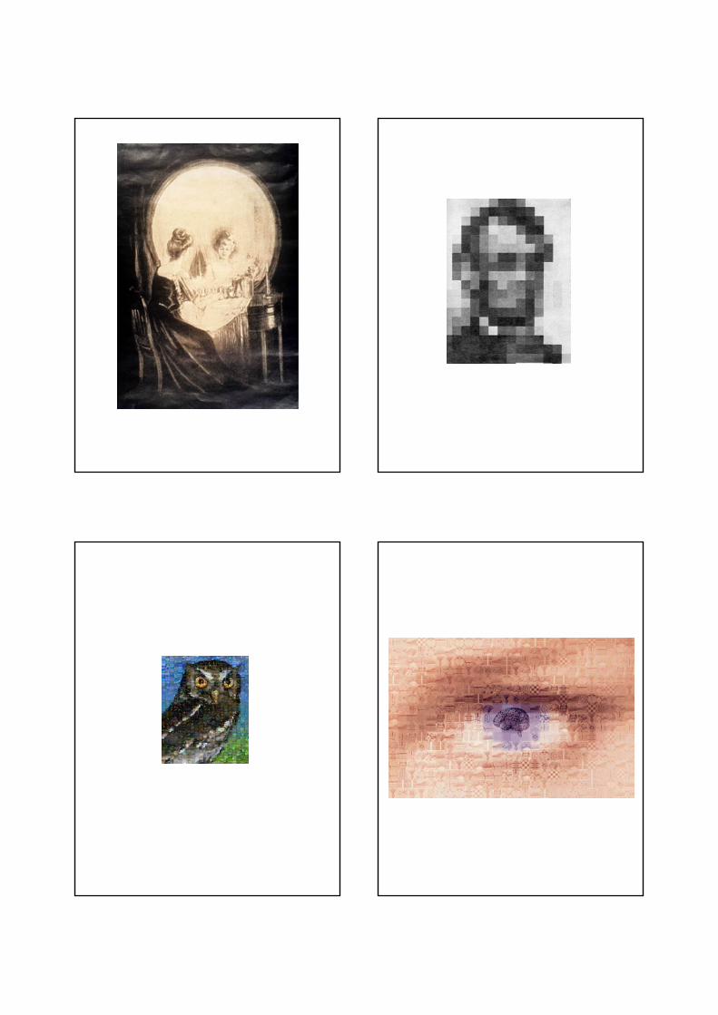
Image Processing
Image Operations in the Frequency Domain
Frequency Bands
Percentage of image power enclosed in circles(small to large) :
90, 95, 98, 99, 99.5, 99.9
Image Fourier Spectrum
Blurring - Ideal Low pass Filter
90% 95%
98% 99%
99.5% 99.9%
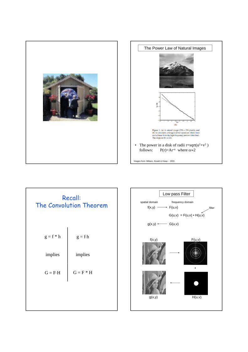
The Power Law of Natural Images
• The power in a disk of radii r=sqrt(u2+v2 ) follows: P(r)=Ar-α where α≈2
Images from: Millane, Alzaidi & Hsiao - 2003
Recall:The Convolution Theorem
g = f * h g = f⋅h
implies implies
G = F⋅H G = F * H
Low pass Filter
f(x,y) F(u,v)
g(x,y) G(u,v)
G(u,v) = F(u,v) • H(u,v)
spatial domain frequency domain
filter
•
f(x,y) F(u,v)
H(u,v)g(x,y)
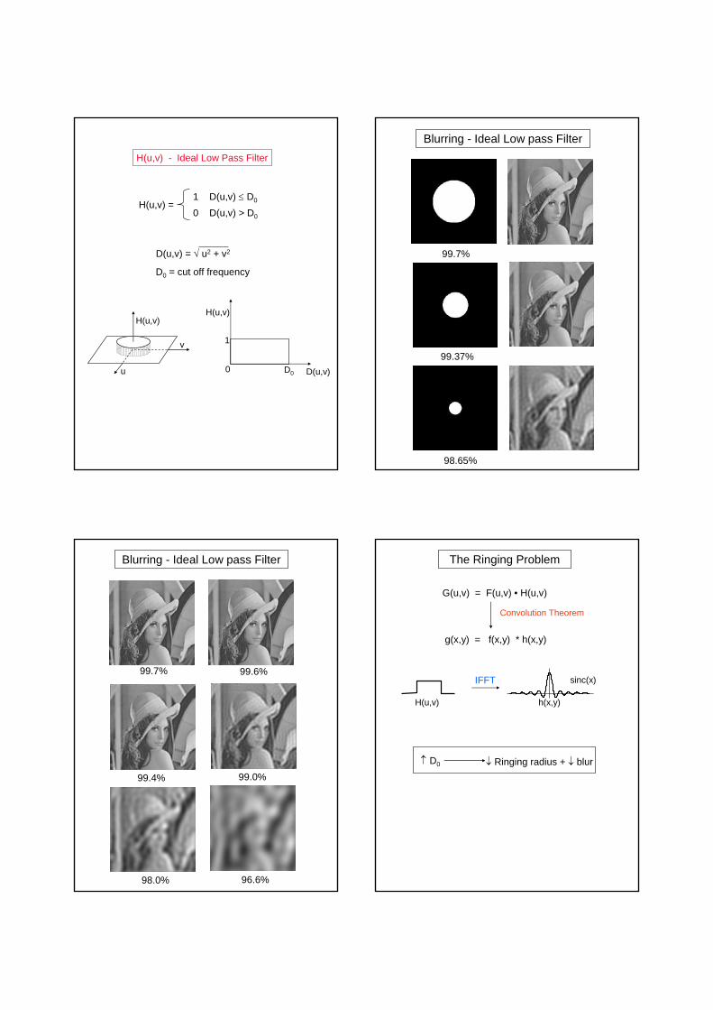
H(u,v) - Ideal Low Pass Filter
u
v
H(u,v)
0 D0
1
D(u,v)
H(u,v)
H(u,v) = 1 D(u,v) ≤ D0
0 D(u,v) > D0
D(u,v) = √ u2 + v2
D0 = cut off frequency
Blurring - Ideal Low pass Filter
98.65%
99.37%
99.7%
98.0%
99.4%
99.7%
Blurring - Ideal Low pass Filter
99.0%
96.6%
99.6%
The Ringing Problem
G(u,v) = F(u,v) • H(u,v)
g(x,y) = f(x,y) * h(x,y)
Convolution Theorem
sinc(x)
h(x,y)H(u,v)
↑ D0 ↓ Ringing radius + ↓ blur
IFFT

The Ringing Problem
0 50 100 150 200 2500
50
100
150
200
250
Freq. domain
Spatial domain
H(u,v) - Gaussian Filter
D(u,v)0 D0
1
H(u,v)
uv
H(u,v)
D(u,v) = √ u2 + v2
H(u,v) = e-D2(u,v)/(2D20)
Softer Blurring + no Ringing
e/1
Blurring - Gaussain Lowpass Filter
96.44%
98.74%
99.11%
The Gaussian Lowpass Filter
Freq. domain
Spatial domain
0 50 100 150 200 250 3000
50
100
150
200
250
300

Blurring in the Spatial Domain:
Averaging = convolution with 1 11 1
= point multiplication of the transform with sinc:
0 50 1000
0.05
0.1
0.15
-50 0 500
0.2
0.4
0.6
0.8
1
Gaussian Averaging = convolution with 1 2 12 4 21 2 1
= point multiplication of the transform with a gaussian.
Image Domain Frequency Domain
Image Sharpening - High Pass Filter
H(u,v) - Ideal Filter
H(u,v) = 0 D(u,v) ≤ D0
1 D(u,v) > D0
D(u,v) = √ u2 + v2
D0 = cut off frequency
0 D0
1
D(u,v)
H(u,v)
u
v
H(u,v)
H(u,v)
D(u,v)0 D0
1
D(u,v) = √ u2 + v2
High Pass Gaussian Filter
u
v
H(u,v)
H(u,v) = 1 - e-D2(u,v)/(2D20)
e/11−
High Pass Filtering
Original High Pass Filtered

High Frequency Emphasis
Original High Pass Filtered
+
=
High Frequency Emphasis
Emphasize High Frequency.Maintain Low frequencies and Mean.
(Typically K0 =1)
H'(u,v) = K0 + H(u,v)
0 D0
1
D(u,v)
H'(u,v)
High Frequency Emphasis - Example
Original High Frequency Emphasis
Original High Frequency Emphasis
High Pass Filtering - Examples
Original High pass Emphasis
High Frequency Emphasis +
Histogram Equalization

Band Pass Filtering
H(u,v) = 1 D0- ≤ D(u,v) ≤ D0 +0 D(u,v) > D0 +
D(u,v) = √ u2 + v2
D0 = cut off frequency
u
v
H(u,v)
0
1D(u,v)
H(u,v)
D0- w2
D0+w2
D0
0 D(u,v) ≤ D0 -w2
w2
w2
w2
w = band width
H(u,v) = 1 D1(u,v) ≤ D0 or D2(u,v) ≤ D0
0 otherwise
D1(u,v) = √ (u-u0)2 + (v-v0)2
D0 = local frequency radius
Local Frequency Filtering
u
v
H(u,v)
0 D0
1
D(u,v)
H(u,v)
-u0,-v0 u0,v0
D2(u,v) = √ (u+u0)2 + (v+v0)2
u0,v0 = local frequency coordinates
H(u,v) = 0 D1(u,v) ≤ D0 or D2(u,v) ≤ D0
1 otherwise
D1(u,v) = √ (u-u0)2 + (v-v0)2
D0 = local frequency radius
Band Rejection Filtering
0 D0
1
D(u,v)
H(u,v)
-u0,-v0 u0,v0
D2(u,v) = √ (u+u0)2 + (v+v0)2
u0,v0 = local frequency coordinates
u
v
H(u,v)
+
+ =
=
Additive Noise Filtering
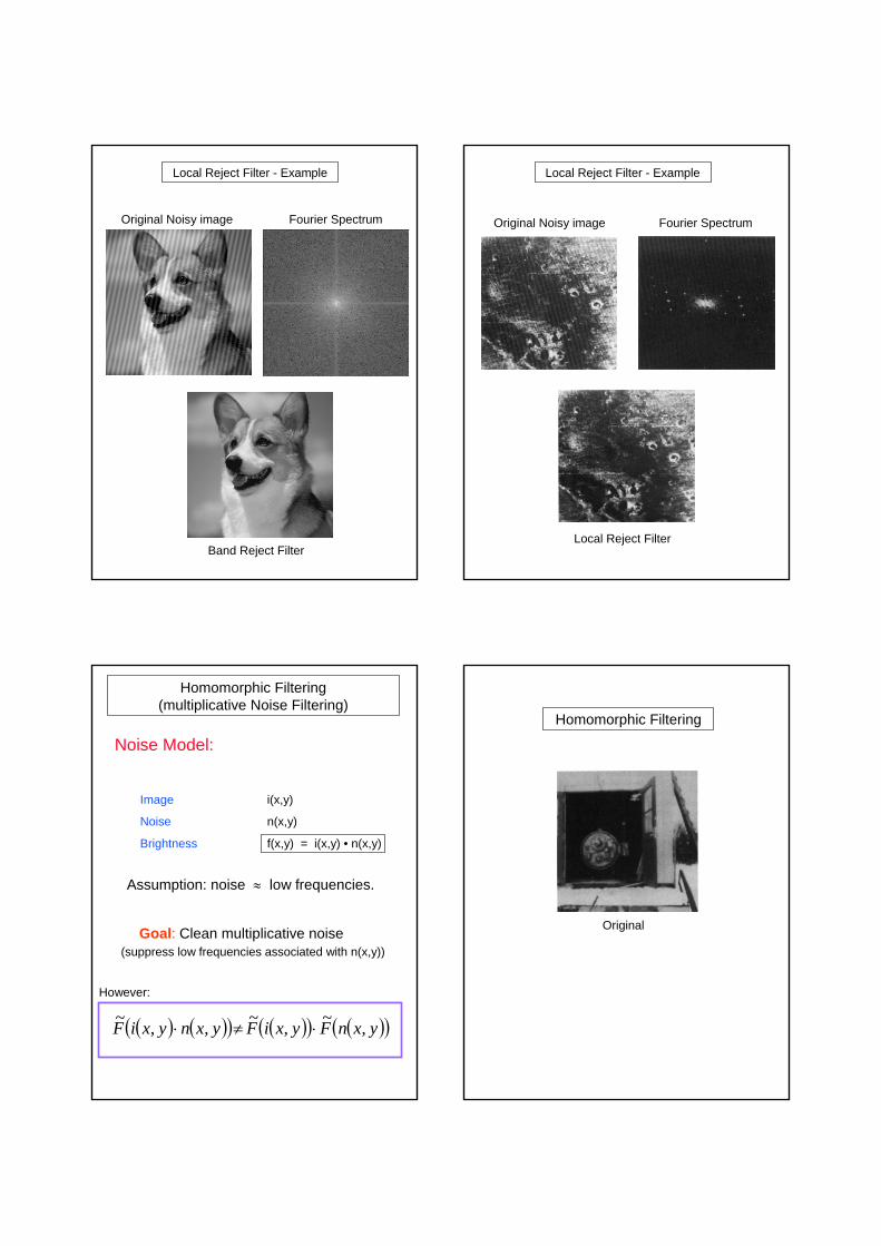
Local Reject Filter - Example
Original Noisy image Fourier Spectrum
Band Reject Filter
Local Reject Filter - Example
Original Noisy image Fourier Spectrum
Local Reject Filter
Homomorphic Filtering (multiplicative Noise Filtering)
Noise Model:
Image
Noise
Brightness
i(x,y)
n(x,y)
f(x,y) = i(x,y) • n(x,y)
Assumption: noise ≈ low frequencies.
(suppress low frequencies associated with n(x,y))Goal: Clean multiplicative noise
( ) ( )( ) ( )( ) ( )( )yxnFyxiFyxnyxiF ,~,~,,~ ⋅≠⋅
However:
Homomorphic Filtering
Original

Surface Reflectance i(x,y)
Illumination n(x,y)
Homomorphic Filtering - Example
Reflectance Model:
Brightness f(x,y) = i(x,y) • n(x,y)
Assumptions:
Illumination changes "slowly" across sceneIllumination ≈ low frequencies.
Surface reflections change "sharply" across scenereflectance ≈ high frequencies.
Illumination Reflectance Brightness
Goal: Determine i(x,y)
Perform:
z(x,y) = log(f(x,y))
I(u,v) + N(u,v)
Apply low attenuating filter H(u,v)
S(u,v) = H(u,v)•Z(u,v)-1
i'(x,y) + n'(x,y)
g(x,y) = exp(s(x,y))
Homomorphic Filtering:
log FFT-1FFT H(u,v) expimage image
log(i(x,y) • n(x,y)) = log(i(x,y)) + log(n(x,y))
=
Z(u,v) =
H(u,v)•I(u,v) + H(u,v)•N(u,v)=
s(x,y) =
exp(i'(x,y)) • exp(n'(x,y))=
Homomorphic Filtering
Original Filtered
Homomorphic Filtering
Original Histogram Equalized
Filtered

Homomorphic Filtering
Original Filtered
Computer Tomographyusing FFT
CT Scanners• In 1901 W.C. Roentgen won the Nobel
Prize (1st in physics) for his discovery of X-rays.
Wilhelm Conrad Röntgen
CT Scanners• In 1979 G. Hounsfield & A. Cormack,
won the Nobel Prize for developing the computer tomography.
• The invention revolutionized medical imaging.
1st prototype of CT scanner
Allan M. Cormack
Godfrey N. Hounsfield
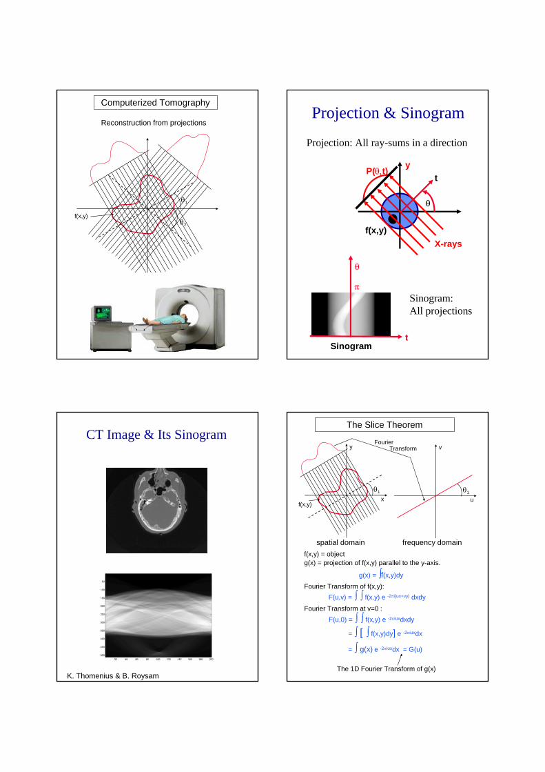
Computerized Tomography
Reconstruction from projections
f(x,y)
θ1
θ2
Projection & Sinogram
Sinogramt
θ
Sinogram: All projections
P(θ,t)
f(x,y)
t
θ
y
x
X-rays
Projection: All ray-sums in a direction
π
CT Image & Its Sinogram
K. Thomenius & B. Roysam
The Slice Theorem
f(x,y)
θ1
x
y
θ1
u
v
spatial domain frequency domainf(x,y) = objectg(x) = projection of f(x,y) parallel to the y-axis.
g(x) = ∫f(x,y)dy
F(u,v) = ∫ ∫ f(x,y) e -2πi(ux+vy) dxdyFourier Transform of f(x,y):
Fourier Transform at v=0 :F(u,0) = ∫ ∫ f(x,y) e -2πiuxdxdy
= ∫ [ ∫ f(x,y)dy] e -2πiuxdx
= ∫ g(x) e -2πiuxdx = G(u)
The 1D Fourier Transform of g(x)
Fourier Transform
u
vF(u,v)
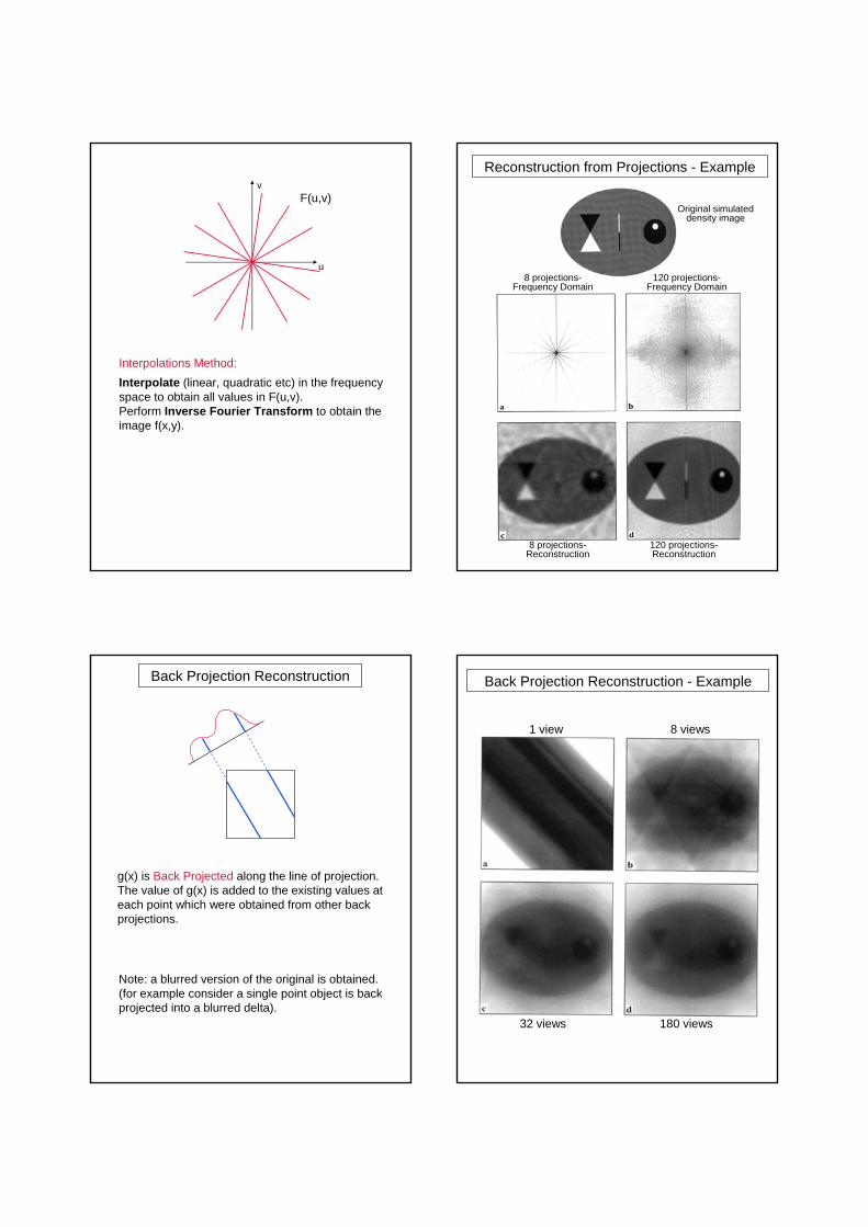
Interpolations Method:Interpolate (linear, quadratic etc) in the frequency space to obtain all values in F(u,v).Perform Inverse Fourier Transform to obtain the image f(x,y).
Reconstruction from Projections - Example
Original simulated density image
8 projections-Frequency Domain
120 projections-Frequency Domain
8 projections-Reconstruction
120 projections-Reconstruction
Back Projection Reconstruction
g(x) is Back Projected along the line of projection.The value of g(x) is added to the existing values ateach point which were obtained from other back projections.
Note: a blurred version of the original is obtained.(for example consider a single point object is backprojected into a blurred delta).
Back Projection Reconstruction - Example
1 view 8 views
32 views 180 views

Filtered Back Projection - Example
1 view 2 views 4 views
8 view 16 views 32 views
180 views
FrequencySpatial
Filter
THE END


