
Louisiana State University Louisiana State University
LSU Digital Commons LSU Digital Commons
LSU Doctoral Dissertations Graduate School
5-28-2020
Identification of Top-down, Bottom-up, and Cement-Treated Identification of Top-down, Bottom-up, and Cement-Treated
Reflective Cracks Using Convolutional Neural Network and Reflective Cracks Using Convolutional Neural Network and
Artificial Neural Network Artificial Neural Network
Nirmal Dhakal
Follow this and additional works at: https://digitalcommons.lsu.edu/gradschool_dissertations
Part of the Civil Engineering Commons
Recommended Citation Recommended Citation Dhakal, Nirmal, "Identification of Top-down, Bottom-up, and Cement-Treated Reflective Cracks Using Convolutional Neural Network and Artificial Neural Network" (2020). LSU Doctoral Dissertations. 5270. https://digitalcommons.lsu.edu/gradschool_dissertations/5270
This Dissertation is brought to you for free and open access by the Graduate School at LSU Digital Commons. It has been accepted for inclusion in LSU Doctoral Dissertations by an authorized graduate school editor of LSU Digital Commons. For more information, please [email protected].

IDENTIFICATION OF TOP-DOWN, BOTTOM-UP, AND
CEMENT-TREATED REFLECTIVE CRACKS USING
CONVOLUTIONAL NEURAL NETWORK AND
ARTIFICIAL NEURAL NETWORK
A Dissertation
Submitted to the Graduate Faculty of the
Louisiana State University and
Agricultural and Mechanical College
in partial fulfillment of the
requirements for the degree of
Doctor of Philosophy
in
The Department of Civil and Environmental Engineering
by
Nirmal Dhakal
M.S.C.E, Louisiana State University, Baton Rouge, U.S., 2016
August 2020

ii
ACKNOWLEDGMENTS
I would like to express my deepest gratitude to my advisor Dr. Mostafa Elseifi for his guidance,
patience, and support throughout the course of my Ph.D. program. His endless support, constant
encouragement, along with academic wisdom counsel motivated me to work hard in the novel and
advanced area of pavement engineering. In addition, I wish to thank Dr. Chester Wilmot and Dr.
Shengli Chen for being on my advisory committee who have taken time and effort to review this
dissertation and for their cooperation, advice and continuous support. I would also like to thank
dean representative Dr. Husam Sadek for his kind support.
I would like to express my appreciation to Louisiana Department of Transportation and
Development and Louisiana Transportation and Research Center for providing me opportunity to
work on this project and helping me in numerous occasions. I am thankful to my fellow research
group members at LSU, Zia UA. Zihan, Mohammad Z. Bashar, and Momen Mousa for their time
and support for the completion of the project. I am also thankful to all the faculty and staff of
Louisiana State University Department of Civil and Environmental Engineering who have been a
part of my research and education over the past two and half years.
I am especially grateful to Dr. Jagannath Upadhyay who supported and guided me as an
elder brother. I would also like to thank Suvash, Sandeep, and Abi for their love and care. I wish
my thanks to all my relatives and friends who have helped me directly and indirectly during my
Ph.D. journey.
I am always indebted to my mother Man Kumari Dhakal and father Padma Raj Dhakal,
and my sisters Darshana and Srijana for their unconditional love and endless support throughout
my life. I would never have made it through without you.

iii
TABLE OF CONTENTS
ACKNOWLEDGMENTS .............................................................................................................. ii
LIST OF TABLES .......................................................................................................................... v
LIST OF FIGURES ....................................................................................................................... vi
ABSTRACT .................................................................................................................................... x
INTRODUCTION ................................................................................................... 1
Background ...................................................................................................................1 Problem Statement ........................................................................................................3
Research Objectives ......................................................................................................3 Research Approach .......................................................................................................4 Research Plan ................................................................................................................5 Scope of Study ............................................................................................................11
LITERATURE REVIEW ...................................................................................... 12 Top-down Cracking in Flexible Pavements ................................................................12
Louisiana Pavement Management System .................................................................15 Image Based Crack Identification Method .................................................................16
Latest Advancements in Image-Based Crack Detection Techniques .........................19 Artificial Neural Network ...........................................................................................24
Finite Element Analysis ..............................................................................................29 Shrinkage in Cement Treated Base .............................................................................49 Summary of Literature Review ...................................................................................52
METHODOLOGY ................................................................................................ 54 CNN and ANN Crack Classification Model ...............................................................54
Finite Element Modeling ............................................................................................72
DEVELOPMENT AND VALIDATION OF CNN AND ANN MODELS .......... 85
CNN Network Performance ........................................................................................85 ANN Training and Performance .................................................................................89
Forward Calculations ..................................................................................................91
FINITE ELEMENT RESULTS ............................................................................. 93 Effect of Tangential Stresses on Tensile Strain ..........................................................93 Critical Locations of Crack Initiation .........................................................................95 Shrinkage Effect on Tensile Stress .............................................................................96
Parametric Studies ......................................................................................................98
ANN BASED WINDOWS APPLICATION....................................................... 102 Step 1: Open Image ...................................................................................................103
Step 2: Image Processing ..........................................................................................104 Step 3: Enter Inputs for ANN Classification ............................................................105 Step 4: Results...........................................................................................................105

iv
Case Study ................................................................................................................106
CONCLUSIONS AND RECOMMENDATIONS .............................................. 120 CNN and ANN Models .............................................................................................120
Finite Element Modelling .........................................................................................121 Recommendations .....................................................................................................123
APPENDIX. CNN CODE FOR IMAGE CLASSIFICATION .................................................. 125
REFERENCES ........................................................................................................................... 127
VITA ........................................................................................................................................... 134

v
LIST OF TABLES
1. Image Data Collection for Each Crack Type ........................................................................... 55
2. Pavement Sections Selected in the Analysis ............................................................................. 56
3. Summary of Coring................................................................................................................... 59
4. Pavement Sections with Bottom-up Cracking .......................................................................... 61
5. Pavement Sections with Cement Treated Reflective Cracking ................................................ 62
6. Detailed Specifications of CNN Model ................................................................................... 69
7. Layer Thickness for Flexible Pavements .................................................................................. 73
8. Tire Dimensions and Maximum Stresses at Different Tire Ribs. ............................................. 77
9. Input Parameters for ALF Test Section Obtained from Model Validation .............................. 82
10. Forward Calculation Results .................................................................................................. 91
11. Description of the Evaluated Mixes ........................................................................................ 99

vi
LIST OF FIGURES
1. Methodology of the Research Approach for Phase 1 ................................................................. 6
2. Pavement Designs for the FE Analysis ..................................................................................... 11
3. (a) Longitudinal Crack in Wheel Path, (b) Field Core .............................................................. 13
4. Primary (Direction 1) and Secondary (Direction 2) Directions for Data Collection ................ 15
5. LADOTD Intranet ..................................................................................................................... 16
6. (a) Convolutional Operator, (b) Max Pooling Operator ........................................................... 20
7. Architecture of Proposed DCNN .............................................................................................. 21
8. CNN Architecture ..................................................................................................................... 22
9. (a) Edge Detection Based Crack Recognition Model, (b) CNN Model Structure for Crack
Detection ..................................................................................................................... 23
10. Illustration of a CNN’s Overall Architecture.......................................................................... 24
11. Example of Feed-Forward Neural Network Structures .......................................................... 26
12. Backpropagation Algorithm.................................................................................................... 27
13. Transfer Functions, (a) Logsig, (b) Tansig, (c) Hardlim ........................................................ 28
14. Traffic loading for 2-D Plane-Strain Models .......................................................................... 35
15. Traffic Loading for Axisymmetric Approach ......................................................................... 36
16. Traffic Loading in 3-D Models ............................................................................................... 37
17. Assumed Loading Cycle ......................................................................................................... 38
18. The 3-D FE Model; (a) Perpetual Pavement Structure and (b) Cross Section ....................... 40
19. (a) Schematic Showing the Meshed Region, (b) Details in Vicinity of Crack ....................... 42
20. System Developed for Two-Step Approach to Finite Element Modeling of Crack Pavement
..................................................................................................................................... 46
21. Contact Stress Distribution due to Tire Loading .................................................................... 47
22. Distribution of Transverse Shear Stress .................................................................................. 48
23. Distribution of Longitudinal Shear Stress............................................................................... 48

vii
24. Drying Shrinkage for Cement Treated Base Mixtures ........................................................... 50
25. Shrinkage Strains for Crushed Stone and Conventional Limestone Mixtures ....................... 50
26. Comparison of Shrinkage Stress and Tensile Strength of Different Mixes ............................ 51
27. Indirect Tensile Strength with (a) 28-day Curing, (b) 56- day Curing, (c) 95% Compaction,
and (d) 100% Compaction .......................................................................................... 52
28. Illustration of Pavement Section Selection for Top-Down Cracking, (a) iVision Platform for
Data Collection, (b) Pavement Image with Top-Down Cracking ............................... 56
29. Acquisition of Field Cores, (a) Marking Core Extraction Location, (b) Coring the Marked
Location, (c) Careful Extraction of Core, (d) Extracted Pavement Core .................... 58
30. Cores Showing Longitudinal Top-down Cracks for Control Sections (a) 829-26, (b) 857-63
..................................................................................................................................... 59
31. Drilled Hole and Fragmented Core ......................................................................................... 60
32. Pavement Section Selection for Bottom-up Cracking ............................................................ 61
33. Pavement Section Selection for Cement Treated Reflective Cracking .................................. 62
34. Illustration of Processed Input Images for (a) Top-down Cracking, (b) Bottom-up Cracking,
and (c) CT Reflective Cracking .................................................................................. 63
35. Intensity Normalization .......................................................................................................... 67
36. CNN’s Overall Architecture ................................................................................................... 68
37. Confusion Matrix for Pattern Recognition ANN .................................................................... 71
38. Inputs for ANN Model ........................................................................................................... 72
39. ANN-based Pattern Recognition Model Structure ................................................................ 72
40. General Layout of FE Model .................................................................................................. 73
41. General Mesh of the FE Model ............................................................................................... 74
42. Pavement Load Contact Area and Boundary Conditions ....................................................... 75
43. (a) Tire Footprint of Dual Tire Assembly; (b) Modeled Contact Area for Dual-Tire Assembly
..................................................................................................................................... 76
44. Amplitudes on Contact Area ................................................................................................... 77
45. Shrinkage Strain at CTB with Time........................................................................................ 78

viii
46. The Louisiana Accelerated Loading Facility .......................................................................... 80
47. Pavement Design and Instrumentation Plan in Experiment III .............................................. 81
48. Measured Longitudinal Strain at the Bottom of Surface Layer after 25,060 Passes .............. 82
49. Measured Vertical Stress at the Bottom of Surface Layer after 47,505 Passes ...................... 83
50. Measured and Calculated Longitudinal Strains at the Bottom of AC Layer .......................... 84
51. Measured and Calculated Vertical Stress at the Bottom of AC Layer ................................... 84
52. Confusion Matrices for Raw Pavement Images for (a) Testing, (b) Validation for CNN
Model .......................................................................................................................... 86
53. Confusion Matrices for 2D Images for (a) Testing, (b) Validation for CNN Model............. 87
54. Confusion Matrices for 2D and 3D Images for (a) Testing, (b) Validation for CNN Model 88
55. Confusion Matrices for the Pattern Recognition System for Training, Validation, and Testing
for ANN Model ........................................................................................................... 90
56. ANN Model Performance ...................................................................................................... 91
57. Tensile Strains at Pavement Surface and Bottom of AC Layer due to Vertical and Tangential
Stresses ........................................................................................................................ 94
58. Tensile Strain Distribution at (a) Asphalt Surface, (b) Bottom of AC Layer .................. Error!
Bookmark not defined.
59. Tensile Stresses due to Shrinkage ........................................................................................... 97
60. Effect of Asphalt Concrete Layer Thickness on Tensile Strain .............................................. 98
61. Effect of Surface Mix Type on Tensile Strains at Pavement Surfaces ................................... 99
62. Tensile Stress at Cement Treated Base Layer due to Shrinkage for Different Test Specimens
................................................................................................................................... 101
63. ANN Interface for Crack Classification ............................................................................... 102
64. CNN and ANN Application for Crack Classification ........................................................... 103
65. First Step to Browse and Open Pavement Image.................................................................. 103
66. Image Processing Procedure (a) Loading Image, (b) Processed Image ................................ 104
67. Illustration of Crack Classification using ANN Interface ..................................................... 105

ix
68. CNN Classification Results for Section 015-31 ................................................................... 107
69. CNN and ANN Classification Results for Section 014-06 ................................................... 108
70. CNN and ANN Classification Results for Section 027-04 ................................................... 109
71. CNN and ANN Classification Results for Section 058-02 ................................................... 110
72. CNN and ANN Classification Results for Section 262-03 ................................................... 110
73. CNN and ANN Classification Results for Section 266-01 ................................................... 111
74. CNN and ANN Classification Results for Section 829-26 ................................................... 112
75. CNN and ANN Classification Results for Section 857-63 ................................................... 113
76. CNN and ANN Classification Results for Section 011-04 ................................................... 114
77. CNN and ANN Classification Results for Section 003-10 ................................................... 115
78. CNN and ANN Classification Results for Section 015-05 ................................................... 116
79. CNN and ANN Classification Results for Section 010-06 ................................................... 117
80. CNN and ANN Classification Results for Section 424-08 ................................................... 118
81. CNN and ANN Classification Results for Section 426-01 ................................................... 119

x
ABSTRACT
The objective of this study was to formulate a Convolutional Neural Networks (CNN) model and
to develop a decision-making tool using Artificial Neural Networks (ANN) to identify top-down,
bottom-up, and cement treated (CT) reflective cracking in in-service flexible pavements. The
CNN’s architecture consisted of five convolutional layers with three max-pooling layers and three
fully connected layers. Input variables for the ANN model were pavement age, asphalt concrete
(AC) thickness, annual average daily traffic (AADT), type of base, crack orientation, and crack
location. The ANN network architecture consisted of an input layer of six neurons, a hidden layer
of ten neurons, and a target layer of three neurons. The developed CNN model was found to
achieve an accuracy of 93.8% and 91.0% in the testing and validation phases, respectively. The
ANN based decision-making tool achieved an overall accuracy of 92% indicating its effectiveness
in crack identification and classification.
In the second phase of the study, the flexible pavement responses under a dual tire assembly
were analyzed to identify the critical stress mechanisms for bottom-up and top-down cracking.
Higher tensile strains were observed to occur underneath the tire ribs than away from them
supporting the argument that both surface initiated and bottom-up fatigue cracking develop in or
near the wheel paths. The incorporation of surface transverse tangential stresses increased the
surface tensile strains near the tire ribs by approximately 68%, 63%, and 53% respectively for low,
medium, and high volume flexible pavements indicating an increased potential for the initiation
and development of top-down cracking when tangential stresses are considered. In contrast, this
effect was observed to be minimal for the tensile strains at the bottom of the asphalt layer, which
are the main pavement responses used in the prediction of fatigue cracking.

xi
Shrinkage cracking in cement treated base (CTB) was also modeled in finite element using
displacement boundary conditions. The tensile stresses due to shrinkage strains in the cement
treated base were observed to be comparable to the tensile strength of CTB at 7 days and higher at
56 days indicating the potential development of shrinkage cracks.

1
INTRODUCTION
Background
Pavement distress detection and quantification is an essential step in managing road networks
and planning for effective rehabilitation and maintenance strategies. The accurate and up-to-
date assessment of pavement conditions is necessary to predict future deterioration rates and
plan for effective preventive maintenance and rehabilitation strategies. State Departments of
Transportation (DOTs) in the United States are routinely using pavement condition evaluation
as an integral part of Pavement Management System (PMS) to provide detailed information of
pavement serviceability. Computer vision and machine learning techniques are successfully
implemented on devices such as Roadware’s Automatic Road Analyzer (ARAN) system, and
Road Measurement Data Acquisition System (ROMDAS) to automate the road survey. In
Louisiana, the pavement network is surveyed biennially using the ARAN system to collect
pavement surface conditions. The ARAN vehicle is equipped with lasers, cameras, sensors,
and computers to collect high definition digital images of pavement right of way, and pavement
surfaces identifying major pavement distresses such as rutting, cracking, faulting, and
macrotexture for both the primary and secondary travel directions (Khattak et al. 2008).
Until recently, pavement cracking was assumed to initiate at the bottom of the AC layer
and propagate upwards to the surface, i.e., bottom-up crack. The loss in structural support due
to excessive loading conditions, inadequate design and construction, and pavement distresses
such as stripping are the major causes of bottom-up cracking. In the past two decades, the
opposite mode of crack initiation and propagation (top-down) gained significant attention
amongst researchers and pavement practitioners. The literature suggests that longitudinal top-
down cracks usually appear in the wheel paths due to high surface horizontal tensile stresses
due to tire loads while other forms of longitudinal cracks are usually bottom-up. Until now,
the field characterization of these cracks have not been well established as compared to fatigue
2
cracking, which initiates at the bottom of the AC layer. The accurate and up-to-date detection
and characterization of pavement cracks would help highway agencies and state DOTs to set
up a more accurate schedule and budget for repair of these cracks.
The recent advancements in image acquisition and processing and machine learning
techniques have proven image-based technology as a promising tool to assess flexible
pavements in terms of surface cracking. Recently, Convolutional Neural Network (CNN)
models have been efficiently implemented in pavement crack classification with minimal
image processing. CNN is a type of Artificial Neural Network (ANN), which uses images as
inputs to extract the target features as outputs for classification (Tong et al. 2017). The
architecture of CNN is typically structured with convolutional, pooling, and fully connected
layers that can analyze the shape change complexity of the pavement cracks (Tong et al. 2017
and Li et al. 2018).
In this study, a novel method of automatic pavement crack identification was developed
based on the application of CNN. Furthermore, a decision-making tool was developed using
ANN as a secondary screening tool and to cross-validate the image-based classification results
obtained from the CNN model.
The second phase of study assessed the crack controlling mechanisms for top-down,
bottom-up, and cement treated reflective cracks. Specifically, top-down cracking (TDC) has
been a topic of frequent and continuing discussion among pavement researchers in the past two
decades and there is no specific distinction in occurrence of top-down cracking in terms of
climatic zones, pavement thicknesses, location in pavement surface, and modes and orientation.
In addition, the specific causes of top-down cracking are still debated. Finite element models
were constructed to incorporate the vertical as well as surface tangential loading to identify the
specific causes and locations for top-down and bottom-up cracking. Furthermore, the

3
shrinkage strains in cement treated base were modeled to assess the cause for cement treated
reflective cracking.
Problem Statement
The timely identification and characterization of pavement distresses such as cracking, rutting,
and raveling helps highway agencies and DOTs to plan for effective road preventive and
maintenance alternatives and to ensure pavement serviceability and quality. The traditional
manual way of acquiring accurate and up-to-date information of pavement distresses is labor
intensive, time consuming, and unsafe. Yet, the advancement in image acquisition and storage
techniques such as high resolution cameras, aerial photo cameras, and laser imaging
technologies have made it safer and easier to capture and collect real time pavement images
for distress identification and analysis, especially for state DOTs. In recent years, researchers
have successfully analyzed these high quality pavement images to detect and gather significant
amount of features related to pavement distresses such as surface cracking.
Pavement cracks can be differentiated as top-down or bottom-up based on the initiation
and propagation phases of these cracks. The treatment and repair of these distresses is entirely
different. None of the previous studies were able to differentiate between top-down and
bottom-up cracking without destructive tool such as coring. It would be beneficial for state
agencies to differentiate between these cracks based on non-destructive approaches such as
machine learning and computer vision.
Research Objectives
The research objective was twofold. First, the study developed a tool to identify and classify
top-down, bottom-up, and cement-treated reflective cracking in in-service flexible pavements
without core extraction or other destructive tool. To achieve this objective, an image-based
CNN model was developed that analyze pavement surface images. Furthermore, a one-step

4
decision-making tool was developed using ANN to cross validate the crack classification
obtained from the imaged-based CNN. Second, finite element models were developed to
identify the causes and critical locations of each crack types. This was achieved using a
commercial FE software ABAQUS. To achieve the objectives of this study, the following
questions were answered.
What are the benefits of crack distress identification and classification?
What are the causes of top-down, bottom-up, and cement treated reflective cracking in
flexible pavements?
How do three different types of crack differ in terms of initiation, growth, and
orientation?
What are the implications of machine learning and computer vision in pavement
applications?
How do the neural network models differentiate between the crack types?
Research Approach
To achieve the objectives of this study, the proposed research activities were divided into two
phases. A comprehensive literature review was conducted as Task 1 to complete the tasks of
each phases. Task 1 is described under the heading ‘Research Plan’.
Phase 1.
Task 2: Selection of pavement types containing different crack types for analysis.
Task 3: Develop CNN model for crack classification using pre-processed images.
Task 4: Develop a decision-making ANN model as a secondary screening tool for
developed CNN.

5
Phase 2:
Task 5: Develop finite element models simulating the pavement loading to identify
the causes and critical locations of different crack types.
Task 6: Analysis of FE modeling results.
Research Plan
Task 1: Literature Review
A comprehensive literature review was conducted to review following topics:
Top-down cracking in flexible pavements,
Louisiana pavement management system,
Image-based crack identification methods,
Latest advancements in image-based crack detection techniques,
Artificial neural network,
Finite element modeling of pavement structure, and
Finite element analysis of top-down, bottom-up, and cement treated reflective
cracking.
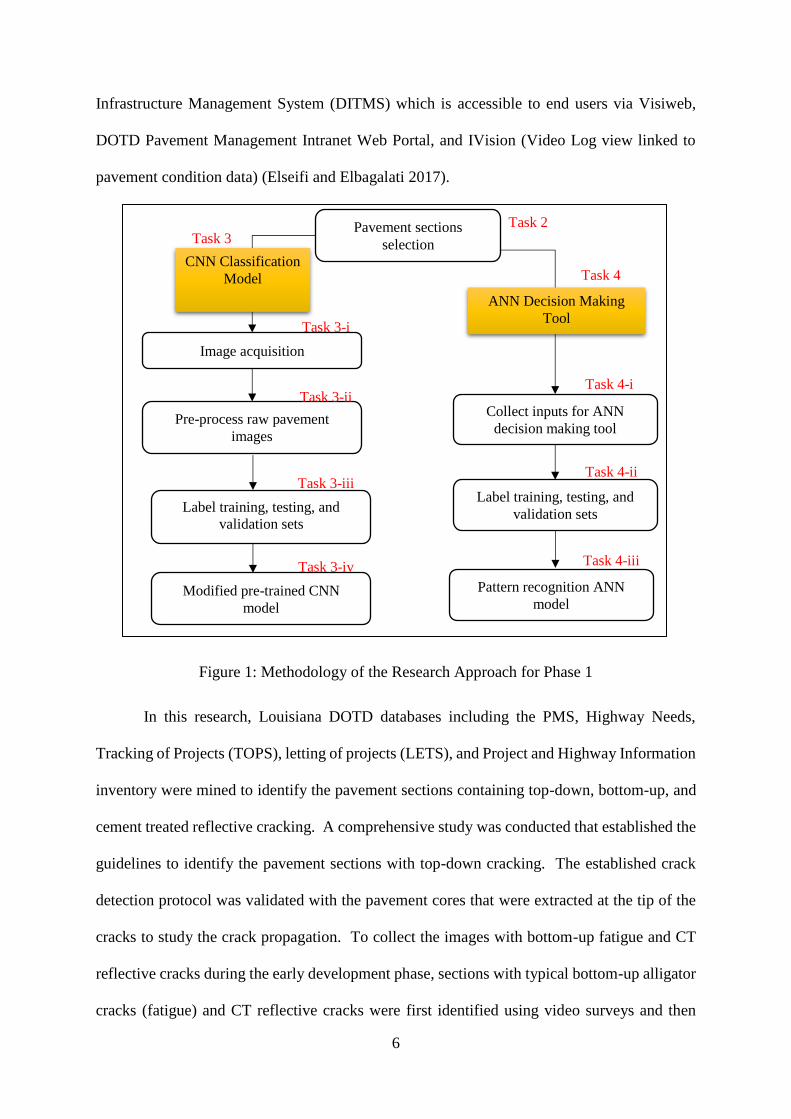
Phase 1 - The research approach adopted in Phase 1 is illustrated in Figure 1.
Phase 1 - Task 2: Pavement Sections Selection
The pavement network in Louisiana is surveyed every two years using the Automatic Road
Analyzer (ARAN®) system that provides a continuous assessment of the road network. The
road survey vehicle is equipped with lasers, cameras, sensors, and computers to collect high
definition digital images of pavement right of way, and pavement surfaces indicating the major
pavement distresses such as rutting, cracking, faulting, IRI, and macrotexture for both primary
and secondary travel directions (Khattak et al. 2008). The collected data is stored using a
Structure Query Language (SQL) enterprise database used by Deighton Transportation
6
Infrastructure Management System (DITMS) which is accessible to end users via Visiweb,
DOTD Pavement Management Intranet Web Portal, and IVision (Video Log view linked to
pavement condition data) (Elseifi and Elbagalati 2017).
Figure 1: Methodology of the Research Approach for Phase 1
In this research, Louisiana DOTD databases including the PMS, Highway Needs,
Tracking of Projects (TOPS), letting of projects (LETS), and Project and Highway Information
inventory were mined to identify the pavement sections containing top-down, bottom-up, and
cement treated reflective cracking. A comprehensive study was conducted that established the
guidelines to identify the pavement sections with top-down cracking. The established crack
detection protocol was validated with the pavement cores that were extracted at the tip of the
cracks to study the crack propagation. To collect the images with bottom-up fatigue and CT
reflective cracks during the early development phase, sections with typical bottom-up alligator
cracks (fatigue) and CT reflective cracks were first identified using video surveys and then
Image acquisition
Label training, testing, and
validation sets
Collect inputs for ANN
decision making tool Pre-process raw pavement
images
Label training, testing, and
validation sets
Pattern recognition ANN
model Modified pre-trained CNN
model
CNN Classification
Model
ANN Decision Making
Tool
Pavement sections
selection
Task 2 Task 3
Task 4
Task 3-i
Task 3-ii
Task 3-iii
Task 3-iv
Task 4-i
Task 4-ii
Task 4-iii

7
projected back to previous year’s survey. The ARAN vehicle that used to collect 2D pavement
images began to collect 3D pavement images starting from the year 2017. For top-down and
CT cracking images, the pavement sections were selected to include 2D pavement images with
cracks that initiated on or before 2016 and 3D pavement images with cracks that initiated in
the year 2017. However, as the images with bottom-up cracking requires projection to previous
year’s survey, the selected pavement sections consisted of 2D images only.
Phase 1 - Task 3: Development of Convolutional Neural Network Classification Model
A convolutional neural network (CNN) model was developed using deep learning method. The
model was built by modifying a pre-trained CNN model known as AlexNet which is widely
recognized for image classification. AlexNet which was developed and trained on a massive
database containing millions of images was used as feature generation for pavement images.
The modified CNN model was developed to classify both 2D and 3D images. The development
of CNN model consisted of four major tasks as described hereunder.
Task 3-i. Image Acquisition
The images for analysis of the pavement cracks were extracted from the Louisiana PMS
inventory. As previously noted, the road network in Louisiana is surveyed every two years
using the ARAN system, which acquires continuous high definition digital images of the
pavement surface. The images are stored in 8-bit color graphics, which provides 256 distinct
levels of gray in which the pixel with a value of 0 is completely black and a pixel with value
of 255 is completely white. The 8-bit gray scale image is easy to manipulate and enhance the
speed of image processing tools. The acquired images consisted of 2D and 3D images for top-
down and cement-treated cracks. However, only 2D images were collected for bottom-up
cracks due to the unavailability of 3D pavement images.
Task 3-ii. Pre-process raw pavement images

8
The pavement images collected by the ARAN system consists of random backgrounds
including pavement surface texture, poor background illumination, roughness, patches, spots,
stains, raveling, and road markings. This task involved the application of different
enhancement and mathematical operations on the image in order to enhance the visibility of
particular features such as pavement cracks. As 2D and 3D pavement images differ in terms
of image resolution, pavement noise, and background illumination, appropriate filtering and
image processing techniques were selected for pavement noise reduction and crack
enhancement for each types of images.
Task 3-iii. Label training, testing, and validation sets
The data set consisting of about 200 2D pavement images of size about 2500 x 4000, and about
150 3D images of size approximately 1000 x 1600 were collected from the LaDOTD PMS
database. These images were pre-processed using an automated preprocessing tool as
mentioned in Task 3-ii. The image data were randomly divided into 60%, 15%, and 25% for
training, testing, and validation respectively.
Task 3-iv. Modify pre-trained AlexNet model
The labeled pavement images were used as training, testing, and validation sets in a modified
pre-trained CNN. Typical CNN models consist of convolutional layers, max pooling layers,
and fully connected layers. The modified network consisted of 5 convolutional layers with 3
max-pooling layers and 3 fully connected layers. The CNN architecture also included other
operations namely rectified linear units (ReLU), local response normalization (LRN), and
dropout where ReLU was used as activation function after each convolution layers and first
two fully connected layers, LRN was used before first two pooling layers, and dropout was
used after first two fully connected layers. The softmax layer consisting of three units for
classification of input data was located at the end of the CNN structure. The overall
architecture included 25 layers with 24 connections. The objective function was optimized
9
using stochastic gradient descent (SGD) algorithm which updates the network parameter after
each input during the training process.
Phase 1 - Task 4: Development of Artificial Neural Network Model
Artificial Neural Network (ANN) was utilized to develop a decision-making tool to serve as a
secondary screening tool. The developed ANN model was used to cross-validate the image-
based classification results obtained from the CNN model. This task consisted of three sub-
tasks as described below.
Task 4-i. Collect Inputs for ANN Decision Making Tool
The inputs related to pavement conditions and crack properties were collected to develop the
ANN-based pattern recognition system. The simplest set of inputs corresponding to the images
were selected and fed to the input layer; these set of inputs does not require any optimization
analysis to be conducted. The input set consisted of six different variables including pavement
age, base type, AADT, AC thickness, orientation of cracks, and location of cracks, which are
readily available from the LaDOTD PMS. Each input was divided into different classes and
assigned a numerical value.
Task 4-ii. Label training, testing, and validation sets
The input data collected from Louisiana PMS and corresponding to 150 pavement images was
used in the ANN model. The data was divided into 70% for training, 15% for validation, and
15% for testing. The testing and validation prediction accuracies were presented in terms of
confusion matrices that present the actual and predicted classes in terms of number and
percentage.
Task 4-iii. Pattern recognition ANN model
A multilayered feed forward ANN was used to develop ANN-based pattern recognition system
using a hard-lim transfer function that presents the output as ‘0’ or ‘1’. A scaled conjugate
gradient back-propagation algorithm (trainscg) was used for the network optimization. A

10
commercial software package MATLAB 2019a was used to process all the data and to develop
the decision making ANN tool. The six inputs for the model were incorporated into the ANN
with six neurons in the input layer and the corresponding prediction classes were incorporated
into the ANN with three neurons in the target layer. The correlations between the inputs and
targets were established with a hidden layer consisting of ten neurons that was connected to
each neuron in input and target layers. An iterative process was used to identify the number of
neurons in the hidden layer such that least number of hidden neurons are selected without
affecting the network performance.
Phase 2 - Task 5: Develop and Validate Finite Element Models
Three dimensional finite element (FE) models were constructed to study the stress distribution
at various depths of pavement due to vehicular loading. The three dimensional approach can
accurately model the pavement structure and loading pattern. The commercial software
ABAQUS was used to simulate a dual-tire assembly loading. The quasi viscoelastic nonlinear
analysis was performed to study the time-dependent responses of the pavement structure to
vehicle loading. Rectangular contact areas were defined in order to accurately simulate the
exact geometry of the loading area and tire movement over the pavement surface. The
symmetrical models were constructed as a combination of pavement layers and surrounding
ground. The AC layer behavior was simulated using a viscoelastic constitutive model while
the base and subbase layers were simulated using elastic constitutive models. The FE model
were validated using the field data before obtaining the outputs.
Phase 2 - Task 6: Analysis of Results
The developed models were used to identify the critical locations of crack initiation for each
crack types. Tensile strain distribution at surface and bottom of AC layer was computed to
identify critical locations and specific cause of pavement cracking. Three flexible pavements
were simulated to study the effect of pavement layer thicknesses on stress distribution, see

11
Figure 2. The effect of shrinkage strains on potential crack development was studied by
simulating displacements corresponding to the strains at different time period.
Figure 2: Pavement Designs for the FE Analysis
Scope of Study
The primary objective of the study was to identify and classify top-down, bottom-up, and
cement treated (CT) reflective cracking in in-service flexible pavements without the need for
core extraction or other destructive tools. To achieve this objective, an image-based CNN
model was developed that analyze pavement surface images. Furthermore, a one-step decision-
making tool was developed using ANN to cross-validate the crack classification obtained from
the imaged-based CNN model.
The study also identified the specific causes and locations of top-down, bottom-up, and
cement treated reflective cracks through developed finite element models. The developed
models were validated using field data and incorporated vertical as well as surface tangential
loading for accurate assessment of the crack controlling mechanisms. Furthermore, shrinkage
in cement treated base with time was simulated to obtain the tensile stresses at CTB and at the
bottom of the asphalt layer.
12
LITERATURE REVIEW
This chapter provides a comprehensive literature review of image based convolutional neural
network classification of pavement images and pattern based artificial neural network
classification methods. The chapter also provides overview of previous studies conducted to
characterize the top-down cracking in flexible pavements. A comprehensive literature review
on finite element methods to model pavement structure and apply tire loading on pavement
surface is also performed. Finally, the chapter outlines the shortcomings in the review of
previous studies.
Top-down Cracking in Flexible Pavements
In the past, pavement cracking was assumed to initiate at the bottom of the AC layer and
propagate upwards to the surface, i.e., bottom-up crack. Yet, the opposite mode of crack
initiation and propagation gained a significant attention amongst researchers and pavement
practitioners in the past two decades. Literature suggest that the longitudinal top-down cracks
usually appear at wheel paths due to high surface horizontal tensile stresses due to tire loads
while other forms of longitudinal cracks are usually bottom-up. Figure 3 presents pavement
surface and a core with top-down cracking in a flexible pavement.
Three main stages of crack propagation have been described by Svasidisant et al.
(2002). The single short longitudinal cracks appear just outside the wheel path in the pavement
surface in the first stage. In the second stage, sister cracks develop parallel to and within 0.3
to 1.0 meters from the original cracks and the short longitudinal cracks in the pavement surface
grow longer. Over time, the cracking reaches a third stage where the parallel longitudinal
cracks get connected via short transverse cracks (Svasidisant et al. 2002).
Myers et al. also reported the surface cracks to initiate just outside the wheel path and
the cracks propagate to depths ranging from just under top surface to the full depth of asphalt

13
concrete layer. The authors considered a wide range of AC thicknesses in their study which
ranged from 50 to 200 mm (2 to 8 inches). The time frame for the initiation of the surface
cracking was reported to be five to ten years following construction. These cracks were
observed to appear as longitudinal with widths of about 3 to 4 mm (0.12 to 0.16 inches) which
decreased as the crack penetrated the AC layer. The total crack depths were noted to range
from about 25 mm (1 inch) form pavement surface to the entire depth of the AC layer (Myers
et al. 1998).
(a) (b)
Figure 3: (a) Longitudinal Crack in Wheel Path, (b) Field Core
Stuart et al. reported the transverse bottom-up cracking to start in the wheel path area
on their study on bottom-up fatigue cracking (Stuart et al. 2001). The location of these cracking
were noted to be the outer edges of the wheel paths where the pavement surface has a high
curvature. The authors also assessed the effect of temperature on cracking; the fatigue cracks
were smaller at 28°C than at 19 and 10°C. This indicates that crack initiation and propagation
varies with the pavement temperature.
The time period for the appearance of surface cracking has been reported to be very
versatile ranging from one year to ten years from the construction. Svasidisant et al. (2002)

14
observed that the surface cracking penetrated through the entire depth of asphalt layers in a 15
year old pavement consisting of a rubblized base. However, the surface cracks propagated
through the full depth of surface layers but only about 50% and 20% respectively through the
intermediate and base layers in the 9 to 10 years old pavements with the similar base structure
(Svasidisant et al. 2002).
A study for the Washington State Department of Transportation discovered that thick
asphalt concrete was also susceptible to top-down cracking (Uhlmeyer et al. 2000). The
authors concluded that top-down cracking would randomly stretch, especially for asphalt layers
with thicknesses surpassing 160 to 180 mm. The observed performance years before the TDC
occurred varies from 1 to 5 years (Japan), 3 to 5 years (France), 5 to 10 years (Florida) and up
to 10 years for the UK. Uhlmeyer et al. noted that top-down cracking occurred typically 3 to
8 years following construction of pavement sections that satisfy structural requirements and
were designed for acceptable equivalent single-axle loads.
In the past 25 years, there has been an alarming increase of pavement distress related
to top-down cracking in the longitudinal wheel path of asphalt pavements. Currently, TDC is
a major asphalt pavement distress in Florida, Washington, Colorado, Louisiana, Michigan, and
other states, as well as in many countries abroad. It has been a topic of frequent and continuing
discussion between researchers worldwide, mostly focused on the roles of binder aging,
segregation, thermal gradient within the surface asphalt layer in creating this distress. The
cracking distress is further accelerated because of wheel loads and contact stresses. TDC
identification in the field and consideration in pavement design methods are problematic
compared to fatigue cracking that is assumed to initiate from the bottom of pavement system.
Maintenance and rehabilitation programming for pavement asset management at the network-
level can benefit tremendously if TDC evaluation is feasible as a part of network-level
condition surveys.

15
Louisiana Pavement Management System
In Louisiana, the pavement network is surveyed every two years to collect the pavement surface
conditions. A special vehicle called Automatic Road Analyzer (ARAN) is equipped with
computers, lasers, cameras, and sensors to capture and store high definition digital images of
pavement right of way, and pavement surfaces indicating the major pavement distresses such
as rutting, cracking, faulting, IRI, and macrotexture for both primary and secondary travel
directions. The control sections are divided into log miles in order to provide a reference
location system to the distress data for all pavements. The control section log mile (CSLM)
defines a route by the type of pavement, average annual daily traffic (AADT), lane width,
number of lanes, shoulder type, shoulder width, and surface material. The distress data are
collected and reported for every 1/10th of a mile (Khattak et al. 2008). The cracks are identified
by category of the distress, categorized in terms of severity as low, medium, and high and
labelled with green, yellow, and red colors respectively (LADOTD Pavement Management
System Guide 2006). A specific rule is followed during the collection of right-of-way and
pavement images where the primary direction or direction 1 indicates South to North and West
to East and the secondary direction or direction 2 indicates North to South and Ease to West
(see Figure 4).
Figure 4: Primary (Direction 1) and Secondary (Direction 2) Directions for Data Collection
(Louisiana PMS Guide, 2006)

16
A Structure Query Language (SQL) enterprise database used by Deighton
Transportation Infrastructure Management System (DITMS) is used to store data which is
available to end users via Visiweb, and IVision (Video Log view linked to pavement condition
data), and DOTD Pavement Management Intranet Web Portal (Elseifi and Elbagalati 2017).
The web application with GIS interface known as ‘intranet version of LADOTD’s PMS’ as
shown in Figure 5 which allows end users to access the required data collected form the survey.
Figure 5: LADOTD Intranet
Image Based Crack Identification Method
The early efforts in developing crack extraction algorithms were focused in statistical intensity
thresholding approaches. Till date, this technique has been used by many researchers due to

17
its simplicity and efficacy. Maser in 1987 proposed a threshold-based segmentation for image
analysis by enhancing the image using histogram equalization (Maser 1987). Li et al.
employed a combination of image histogram and projection histogram to separate the non-
distress objects such as road markings, oils, and tire marks from major distresses on flexible
pavements (Li et al. 1991). Koutsopoulos and Downey observed the regression-based
histogram method to provide best results compared to other three intensity thresholding
methods which included Otsu’s method (Otsu 1979), relaxation method, and Kittler’s method
(Kittler and Illingworth 1986). The authors developed image enhancement, segmentation, and
distress classification algorithms to address different distress types in flexible pavements. A
different approach was suggested for image binarization which assigned a value of 0 to 3 to
each pixel based on its probability of belonging to the object (Koutsopoulos and Downey
1993).
Georgopoulos et al. developed an algorithm and used a software ‘APDIS’ to
automatically identify the type, extent, and severity of pavement crackings (Georgopoulos et
al. 1995). Xu and Huang developed an algorithm based on ‘grid cell’ analysis, which divides
the pavement into small cells and a cell is classified as a crack or non-crack based on the
statistical characteristics (Xu and Huang 2003). Wu et al. developed a crack recognition and
segmentation algorithm namely MorphLink-C; the algorithm mainly consisted of two
processes; (a) using morphological dilation transform to group crack fragments and (b) using
thinning transform to connect the fragments (Wu et al. 2014).
Wavelet transforms, edge detection, and texture analysis are three other widely used
techniques in pavement crack detection (Zou et al. 2012). Zhou et al. used wavelet transform
to separate road distresses into high-amplitude wavelet coefficients and pavement noise to low-
amplitude wavelet coefficients before applying statistical functions to detect and segment
cracks (Zhou et al. 2006). Ying and salari proposed a beamlet transform based technique in

18
order to extract linear features such as cracks in pavement after application of an image
enhancement algorithm (Ying and salari 2009). A method based on 2D wavelet continuous
wavelet transform was applied to detect pavement cracks by Subirats et al. (Subirats et al.
2006). A multiscale complex coefficient maps were created before the application of an
algorithm to search wavelet coefficient maximal values and their propagation through the
scales for crack detection. The wavelet transform techniques however has limitation in
detecting high curvature or low continuity cracks (Zou et al. 2012).
In edge detection techniques, algorithms are applied to search and detect edges (defined
as sharp intensity transitions) without any inputs or human interference. Abdel-Qader et al.
used bidimensional empirical mode decomposition (BEMD) smoothing method to remove
noise and applied sobel edge detection technique to detect cracks (Abdel-Qader et al. 2003).
The sobel edge detection technique was observed to produce better results for images with less
irregularities and noise (Ayenu-Prah and Attoh-Okine 2008). Maode et al. employed
morphological operation tools to detect, extract and fill the crack edges. The procedure
consisted of the application of morphological gradient operator with morphological closing
operator after the use of median filter to smooth and enhance pavement image (Maode et al.
2007). The texture analysis techniques employs crack extraction algorithms to separate cracks
from highly textured pavements.
Song et al. presented an algorithm based on Wigner distribution to segment cracks from
complex textured background. This model was adjudged highly effective and better than
Fourier based crack detector in terms of locality and discriminatory power (Song et al. 1995).
In a study by Hu and Zhao a gray-scale and rotation invariant operator called as local binary
pattern (LBP) was used for texture classification and crack detection (Hu and Zhao 2010).
Despite certain improvements in various image processing techniques, researchers still
encounter various challenges in image processing due to texture inhomogeneity of pavement

19
aggregates, random non-crack background noises, spots and stains, oils, road markings and so
forth. These challenges demand further advancement in image preprocessing and thresholding
techniques to precisely assess flexible pavement conditions.
Latest Advancements in Image-Based Crack Detection Techniques
In recent years, there has been a significant improvement in crack recognition, classification,
and characterization approaches that use computer vision techniques. These techniques are
considered as promising approaches to assess the pavement conditions in terms of cracking by
analyzing the pavement images. Koch et al. in their review stated the increasing use of high
level computer vision techniques such as neural models and support vector machines (SVM)
with image processing in segmentation, classification, and feature extraction of pavement
cracks (Koch et al. 2015). Moussa and Hussain used SVM to classify the cracks as transvers,
longitudinal, block, and alligator cracking after the images were segmented using graph cut
segmentation procedure (Moussa and Hussain 2011). Nguyen et al. combined Conditional
Texture Anisotropy (CTA) method of crack segmentation with multi-layer perceptron neural
network and classified the detected defect as cracks, joint, and bridged (Nguyen et al. 2009).
Mokhtari et al. compared four computer-vision based crack detection systems namely
artificial neural network (ANN), k-nearest neighbor, decision tress, and adaptive neuro-fuzzy
inference system (ANFIS). ANN and ANFIS methods were observed to be more accurate in
terms of performance prediction, computation time, and stability of the results and classifiers’
performance (Mokhtari et al. 2016).
The Deep Learning (DL) based computer vision approaches have gained a significant
attention amongst pavement researchers over the past few years, particularly for distress
classification. The four main DL architectures include Restricted Boltzman Machines (RBMs),
Deep Belief Networks (DBNs), Autoencoder (AE), and Deep Convolutional Neural Networks

20
(DCCNs or Deep ConvNets) (Gopalakrishnan et al. 2017). The DCCNs are typically
composed of convolutional, pooling and fully connected layers; a filter bank which is a set of
weights connects units in the feature maps of convolutional layers to local patches in the feature
maps of the input data, the pooling layer units receives the maximum of a local patch of units
in one feature map and also reduces the resolution of feature maps to select the spatial
invariance, and the fully connected layers are like traditional multi-layer perceptron in which
all units in the feature maps are concatenated together into a form of a vector (Li et al. 2018).
Figure 6 illustrates the feature map generation with the convolutional operator (Hoang et al.
2018). The convolutional layer consists of convolution filters and generates same number of
feature maps as that of filters. The pooling layers however contains a stationary filter such that
the convolution areas do not overlap. The pooling layer reduces the image size to improve
computational efficiency and avoid data overfitting. An illustration of pooling operation is
presented in Figure 6 (Hoang et al. 2018).
(a) (b)
Figure 6: (a) Convolutional Operator, (b) Max Pooling Operator (Hoang et al. 2018)
Zhang et al. developed an automatic crack detection DCNN based on the manually
annotated image patches as inputs (Zhang et al. 2016). The dataset consisted of 500 pavement
images of size 3264*2448 collected using a smart phone. The collected pavement images were
sampled to generate one million three-channel (RGB) 99*99 pixel image patches; 640,000
samples were used for training, 160,000 samples were used for validation, and 200,000 samples
were used for training. The developed solution classified the crack and non-crack pixels

21
referred to as positive and negative patches respectively based on a ConvNet trained in square
image patches. The training process was amplified using the rectified linear units (ReLU)
activation function. Figure 7 illustrates the architecture of proposed DCNN (Zhang et al. 2016).
Figure 7: Architecture of Proposed DCNN (Zhang et al. 2016)
Elisenbach et al. developed a convolutional neural network for road crack detection and
named it as RCD net which used same four-block ConvNet at developed by Zhang et al.
(Eisenbach et al. 2017). German Asphalt Pavement Distress (GAPs) dataset was introduced as
an attempt to create a standard benchmarking pavement distress dataset for DL applications
(Gopalakrishnan 2018). A DL approach ASINVOS which consisted of eight convolutional
layers, three max-pooling layers, and three fully-connected layers was implemented to study
the regularization effects on the generalization ability of DCNN; the proposed approach was
observed to outperform the traditional distress detection approaches with higher generalization
ability (Eisenbach et al. 2017). Maeda et al. used object detection CNN for automatic road
distress detection. The images for the proposed approach were acquired using a smartphone
installed in a moving vehicle. The authors also developed a mobile application that captures
600*600 pixels road images by a smartphone mounted on a car (Maeda et al. 2018).
Fan et al. proposed an automated crack detection procedure based on structural
prediction using CNN. The CNN modeled as a multi-label classification problem consisted of

22
four convolutional layers, two max-pooling layers, and there fully-connected layers. The
overall pavement condition was presented by probability map obtained by summing the center
patch structure predictions of the trained CNN applied on all pixels. The proposed method was
observed to be superior compared with other existing methods of crack detection (Fan et al.
2018). The CNN used by the authors is illustrated in Figure 8. The convolutional layers were
with kernel of 3 x 3, stride 1 and zero padding and max pooling was performed with a stride 2
over a 2 x 2 window.
Figure 8: CNN Architecture (Fan et al. 2018)
Wang and Hu employed principal component analysis (PCA) and CNN to classify
pavement cracks as transverse, longitudinal, and alligator by first detecting cracks by
segmenting image into grids after applying PCA to analyze the skeleton of crack (Wang and
Hu 2017). The authors used two different scales of grid (32*32, 64*64) for image
segmentation. The CNN architecture consisted of two convolutional layers, two max-pooling
layers, and one fully-connected layer. The proposed approach was observed to achieve higher
classification accuracy; 97.2%, 97.6%, and 90.1% respectively for longitudinal, transverse, and
alligator cracks.
Hoang et al. performed a study to compare pavement cracking detection using edge
detection technique and convolutional neural network (CNN). The edge detection technique

23
employs the Canny and Sobel algorithms for image processing and are dependent upon the
selection of proper threshold parameters for better accuracy. The models were trained and
validated with 400 images of crack and non-crack labels. Figure 9 presents the edge detection
based crack recognition model and CNN model structure which was trained using the
MATLAB image processing toolbox. The convolutional operations were employed with the
30 number of filters (K). The size of first, second, third, and four convolutional layers were 12
x 12, 8 x 8, 5 x 5, and 3 x 3 respectively while the size was 6 x 6, 4 x 4, 4 x 4, and 3 x 3 for
four pooling layers. The accuracy of CNN, Sobel algorithm, and Canny algorithm were
observed to be 92.08%, 79.99%, and 76.69% respectively (Hoang et al. 2018).
(a)
(b)
Figure 9: (a) Edge Detection Based Crack Recognition Model, (b) CNN Model Structure for
Crack Detection (Hoang et al. 2018)
The testing and validation accuracy of DCCNs is usually dependent upon the training
image dataset. Researchers have suggested in using at least 10,000 images in each class for

24
higher classification accuracy using DL based classification (Liene 2016). In some domains
where acquisition of large dataset is difficult, the use of ‘off-the-shelf’ DCNN features of well-
established DCNN such as AlexNet, resnet, VGG-16, and GoogLeNet have proven to be the
useful tool in classification; these networks are pre-trained using large-scale annotated natural
image datasets. This approach also called as transfer learning enables the learning ability of
pre-trained models trained on large data to deploy on a new domain consisting of a smaller
number of dataset (Gopalakrishnan et al. 2017). Li and Zhao successfully implemented
AlexNet to detect pavement cracks; the authors modified the pre-trained AlexNet with five
convolutional layers, three max-pooling layers and three fully connected layers. The dropout
and local response normalization were implemented, where normalization followed by first
two pooling layers, and dropout was located after first two fully connected layers (Li and Zhao
2019). Figure 10 presents the CNNs overall architecture.
conv# = Convolution; pool# = Pooling; fc# = Full Connection; k# = Kernel of each Operation
Figure 10: Illustration of a CNN’s Overall Architecture (Li and Zhao 2017)
Artificial Neural Network
Artificial Neutral Networks (ANNs) are parallel computing schemes that functions similar to
the mechanism of the human biological nature of neurons and can model complex problems.
ANNs are widely recognized as effective computational modelling tools to solve engineering

25
problems because of the unique features such as non-linearity, noise tolerance in the input data,
adaptability with complicated data patterns, and data generalization capability. These
properties of ANN allows complex data fitting and facilitates the model implementation to
unlearned data (Elseifi and Elbagalati 2017). The generic, accurate, and complex mathematical
models with high capability to simulate numerical model components are developed of solve
complex engineering problems (Karlaftis and Vlahogianni 2011). The learning ability of
genetic flexible training algorithm in ANN allows it to make decisions based on given inputs
(Kim et al. 2014). The ANN provide robust models can be continuously updated with new
data and are more accurate with large database (Plati et al. 2015).
2.5.1. Feed Forward ANN
A feed forward ANN is most frequently used ANN structure for classification problems and
regression analysis. It consists of (a) an input layer ‘i’ that is typically used to train the model
with multiple independent variables, (b) one or more hidden or processing layers ‘j’ that adjust
and update the weights to process the data, and (c) a target layer ‘k’ (Kim et al. 2014). The
processing units called ‘neurons’ are assigned a ‘bias’ and are connected to each other with
each connection assigned a ‘weight’. An example of ANN is presented in Figure 11 (Elseifi
and Elbagalati 2017).

26
Figure 11: Example of Feed-Forward Neural Network Structures (Elseifi and Elbagalati
2017)
2.5.2. Back Propagation Algorithm
A most common algorithm for error optimization in the learning and training phases of ANN
is called back-propagation which calculates the weights and biases to match the desired output
(Elseifi and Elbagalati 2017). Figure 12 illustrates the concept of backpropagation algorithm.
Equation 1 presents the objective function which calculates the error from the network output.
The target of the ANN is to minimize this objective function as in a regular optimization
problem.
E = 1
2 (t − y)2 =
1
2[t − f(w, b, x)]2 (1)
where,
E= error function;
y = network output;
t = target value;
w= weights;
b= biases; and
x= independent variables:

27
Figure 12: Backpropagation Algorithm (Elseifi and Elbagalati 2017)
2.5.3. ANN Transfer Functions
The output of the network training is provided by different activation functions which are
assigned to the weighted input of the neuron. The transfer functions or the activation functions
are the differentiable non-linear functions which allows the neural network to acquire non-
linearity. The logistic sigmoidal function (logsig), tan sigmoidal function (tansig), and
‘hardlim’ are three major transfer functions used in the ANN as shown in Figure 13. The logsig
transfer function produces the output between ‘0’ and ‘+1’, tansig produces the output between
‘-1’ and ‘+1’. The hardlim is the most commonly used activation function and produces the
output between ‘0’ and ‘+1’ which allows the ANN to perform the classification (Elseifi and
Elbagalati 2017).

28
(a) (b)
(c)
Figure 13: Transfer Functions, (a) Logsig, (b) Tansig, (c) Hardlim (Elseifi and Elbagalati
2017)
2.5.4. ANN Forward Calculations
The ANN network can be used as a forward calculation tool once the desired accuracies are
achieved during training, testing, and validation phases. The network assigns proper weights
and biases to the connections and neurons which can be used to perform forward calculation
on new data set. Leverington (2012) presented the general equation of a backpropagation
algorithm. This equation is based on ANN with one output variable, one hidden layer variable,
and a tan-sigmoid transfer function (see Equation 2).
y = (bK + ∑ tansig(bj+ ∑ aiWij)ni1
nj
1 Wjk) (2)
0
0.1
0.2
0.3
0.4
0.5
0.6
0.7
0.8
0.9
1L
ogsi
g(x
)
-1.5
-1
-0.5
0
0.5
1
1.5
tansi
g(x
)
-1
0
1
har
dli
m(x
)

29
where,
k= the model output at layer k;
nj = number of neurons in the hidden layer;
ni = number of neurons in the input layer; and
ai = the input variables
The input vector is multiplied by the weight matrix (Wij) and hidden bias vector (bj) is
added which computes the inputs to the hidden layer (j) at the first step. Then, the outputs of
the hidden layer (j) are calculated by using the activation function which is then multiplied by
the weight vector (Wjk) and added with bias value (bk) to calculate the output vector
(Leverington 2012).
Finite Element Analysis
The oldest method to simulate flexible pavement response to vehicular loading was developed
by Boussinesq in 1885 (Boussinesq 1885), which provided a closed form solution to calculate
stresses, strains, and deflections for a homogeneous, isotropic, linear elastic semi-infinite space
under a point load. Since then, various layered theories and computer programs have been
developed to calculate pavement responses to loading for single and multi-layered systems.
Some effective software programs to solve a layered system problem include VESYS (1977-
1988), ILLI-PAVE (1980), ELSYM5 (1985), KENLAYER (1993), CIRCLY4 (1994), BISAR
(1973-1998), and VEROAD (1993-1999). However, these software are incapable to predict
the actual pavement responses as various factors such as the frequency, contact conditions, and
speed of the loading, the environmental conditions, boundary conditions, material properties,
and interaction between the layers are usually neglected.
The Finite Element (FE) technique can effectively simulate almost all pavement
controlling parameters such as dynamic loading, material properties, viscoelastic and non-

30
linear elastic behavior, joints in the concrete pavements, interaction between the layers,
damping, infinite and stiff foundations, quasi-static analysis, and many more. The use of FE
technique to simulate flexible pavement dates back to 1993 when Zaghloul and White
effectively investigated the effect of load speed and AC properties in rut depth (Zaghloul and
White 1993). The following year, Uddin et al. investigated the effect of discontinuities on
pavement responses using FE techniques (Uddin et al. 1994). In 1999, Shoukry et al. used a
3D FE model to back-calculate the layer moduli of flexible pavements and observed that the
solution of pavement response problem using FE technique does not require the assumptions
made in layered elastic theories (Shoukry et al. 1999).
The level of accuracy of pavement responses in 3D FE models depends on different
factors, including the degree of refinement of the mesh (element dimensions), the order of the
elements (higher order elements usually improve the accuracy), location of the evaluation
(results are more accurate at the Gauss points), appropriate selection of the boundary conditions
and the load discretization process. The present study used a commercial software ABAQUS
CAE, which is an interactive environment used to create finite element models, assign loading
and boundary conditions, submit and monitor ABAQUS jobs, and evaluate results. The
ABAQUS model contains different kinds of objects namely, parts, materials and sections,
assembly, sets and surfaces, steps, loads, boundary conditions, and fields, interaction and their
properties, and meshes.
2.6.1. Finite Element Methods and ABAQUS
The ABAQUS finite element system includes (Simulia, D., ABAQUS theory manual, 2011):
ABAQUS/Standard, a general-purpose finite element program;
ABAQUS/Explicit, an explicit dynamics finite element program;

31
ABAQUS/CAE, an interactive environment used to create finite element models,
submit ABAQUS analyses, monitor and diagnose jobs, and evaluate results; and
ABAQUS/Viewer, a subset of ABAQUS/CAE that contains only the post processing
capabilities of the Visualization module.
The commercial software ABAQUS CAE was used for FE modeling for this project.
ABAQUS/CAE is a complete ABAQUS environment that provides a simple, consistent
interface for creating, submitting, monitoring, and evaluating results from ABAQUS/Standard
and ABAQUS/Explicit simulations (ABAQUS 6.13 2013). The various modules of
ABAQUS/CAE include;
Part, to create individual parts by sketching or importing the geometry,
Property, to create sections and material definitions and assign them to regions of parts,
Assembly, to create and assemble part instances,
Step, to create and define the analysis steps and associated output requests,
Interaction, to specify the interactions between the regions,
Load, to specify loads, boundary conditions and fields,
Mesh, to create and finish element mesh,
Optimization, to create and configure an optimization task,
Job, to submit a job for analysis and monitor the progress,
Visualization, to view analysis results and selected model data, and
Sketch, to create two-dimensional sketches.
Analysis Step and Interaction
The term step in ABAQUS refers to the specific procedure to analyze a job; it provides a
convenient way to capture changes in the loading and boundary conditions of the model,
changes the ways of interaction between the parts, and allows to change the analysis procedure,

32
data output, and various controls (ABAQUS 2013). The two types of steps in ABAQUS
includes the initial step and analyses; the initial step allows to define the boundary conditions,
predefined fields, and interactions that are applicable at the very beginning of the analyses, and
the analyses step allows to perform the required type of analysis.
The interaction module allows to define and manage mechanical and thermal
interactions between the parts or between a parts of a model and surrounding. This module
can be used to define various objects such as contact interactions, elastic foundations, cavity
radiation, pressure penetration, acoustic impedance, inertia, springs and dashpots, and others.
A surface-to-surface contact interaction was used in the developed model for the project. This
interaction defines the contact between two deformable surfaces or between the deformable or
rigid surface. The elastic foundation type of interaction was used for the subgrade surface; this
allows to model the stiffness effects of a distributed support on a surface without actually
modeling the surface (ABAQUS 2013).
2.6.1.2 Load and Boundary Conditions
The load module allows to define and manage loads, boundary conditions, predefined fields
and load cases. Different load types namely, concentrated force, moment, general and shear
surface traction, general shell edge load, inertia relief, and current density can be defined on
the analysis step/s. The amplitude toolset in load module can be used to specify complicated
time or frequency dependencies that can be applied to prescribed conditions (ABAQUS 2013).
The various boundary conditions include, (1) symmetry/antisymmetric/encastre, (2)
displacement/rotation, (3) velocity/angular velocity, (4) acceleration/rotational acceleration,
(5) eulerain mesh motion, and (6) magnetic vector potential. The displacement/rotation
boundary condition which constrain the movement of the selected degrees of freedom to zero
was used as the boundary condition for the present study.

33
2.6.1.3 Elements
The element library of ABAQUS provides a complete geometric modeling capability and
includes continuum elements, infinite elements, membrane and truss elements, beam elements,
shell elements, connector elements (springs and dashpots), special-purpose elements, and
contact elements (ABAQUS 2011). The continuum and spring elements which are used in the
FE model are discussed hereunder.
2.6.1.4 Continuum Elements
The continuum elements are the standard volume elements of ABAQUS and can be composed
of a single homogeneous material or, in ABAQUS/Standard, can include several layers of
different materials to analyze composite solids (ABAQUS 2013). The continuum elements,
particularly quadrilaterals and hexahedra are more accurate if not distorted while triangular and
tetrahedral elements are less sensitive to distortion. These elements are mainly used for linear
analysis and complex nonlinear analysis involving contact, plasticity, and large deformations.
The continuum elements can be of (1) first order (linear) or second order (quadratic)
interpolation elements in one, two, or three dimensions, (2) full or reduced integration; the
reduced integration reduces running time, especially in three dimensions. C3D8R continuum
elements which are 8 node reduced integration linear brick elements with hourglass control
were assigned to the mesh of the developed FE model; the hourglass control prevents the
elements from excessive distortion.
2.6.1.5 Spring Elements
The major attributes of spring elements in ABAQUS are:
can couple a force with a relative displacement,
can couple a moment with a relative rotation in ABAQUS/Standard,
can be linear or nonlinear,

34
can be dependent on temperature and field variable, and
can be used to assign a structural damping factor to form the imaginary part of spring
stiffness.
Three types of spring elements namely SPRING1, SPRING2, and SPRINGA are available in
ABAQUS; SPRING1 can be used to connect nodes and ground acting in fixed direction,
SPRING2 can be used to connect a node with another acting in fixed direction, and SPRINGA
elements can be used to connect two nodes with its line of action being the line joining the two
nodes, so that the line of action can rotate in large-displacement analysis.
2.6.2. Finite Element Approaches in Pavement Analysis
Multi-layered pavement structures can be analyzed using three different kinds of FE
approaches; plain strain, axisymmetric, and three-dimensional.
2.6.2.1 Plane-Strain Approach
The plane-strain approach (2-D) approach cannot accurately simulate the actual traffic
loadings, as line load is used to represent the loading, see Figure 14. However, this approach
is widely used as it requires relatively little computational time and memory (Lytton et al.,
1993). The third dimension of the pavement structure is assumed to have a constant curvature
with respect to the axial direction of the model and has no effect on pavement responses to
traffic loading (Cho et al. 1996).

35
P p
Figure 14: Traffic loading for 2-D Plane-Strain Models (Cho et al. 1996)
2.6.2.2 Axisymmetric Approach
The axisymmetric approach assumes constant properties of the pavement structure on
horizontal planes and considers that the 3D structure is mathematically reduced to a 2D
structure (Cho et al. 1996, Elseifi 2003). This approach uses a cylindrical coordinate system
to solve a 3D problem with a 2D formulation. The limitation of this approach is that the
problems due to dual tire configuration could not be studied as the load can only be modeled
as a single circular load. In addition, the shoulder conditions and discontinuities in the
pavement cannot be modeled using the axisymmetric approach as presented in Figure 15 (Cho
et al, 1996).

36
Figure 15: Traffic Loading for Axisymmetric Approach (Cho et al. 1996)
2.6.2.3 Three-Dimensional Approach
The three dimensional approach can accurately model the pavement structure and loading
pattern. The shoulder conditions, discontinuities in the pavement, boundary conditions and the
foundation can be accurately input in the 3-D approach using special elements such as spring
or pressure elements (Cho et al. 1996). The limitations of this approach is the requirement of
longer computational time and memory, and data preparation for the complex pavement
structure. The level of accuracy of pavement responses in 3D FE models depends on different
factors, such as degree of refinement of the mesh (element dimensions), the order of the
elements (higher order elements usually improve the accuracy), location of the evaluation
(results are more accurate at the Gauss points), appropriate selection of the boundary conditions
and the load discretization process. The three dimensional approach is illustrated in Figure 16.

37
Figure 16: Traffic Loading in 3-D Models (Cho et al. 1996)
2.6.3. Finite Element Modeling of Pavement Structure using ABAQUS
Zaghloul and White performed a dynamic analysis of a flexible pavement by incorporating the
factors neglected by elastic layer analysis such as moving loads, system damping, and
viscoelastic and plastic material behaviors into a three dimensional FE model constructed using
ABAQUS (Zaghloul and White 1993). The FE model was meshed finely in the region of load
path (mesh with 4.44-in. spacing was used in X direction) while relatively coarse mesh (mesh
with 22.2-in. spacing was used in X and Y directions) was generated away from it. The
boundary conditions representing the vertical friction and lateral passive pressure were applied
at the pavement edge parallel to the traffic direction (Y-axis). The length of the sections in the
direction parallel to X-axis was selected to be 600 in. to reduce any edge effect error during the
analysis. The asphalt layer was modeled as viscoelastic material, Drucker-Prager model was
used for the granular materials which assumes the materials to behave as elastic materials for
low stress level and the Cam-Clay model which uses a strain rate decomposition was used for
clays. As presented in Figure 17, a combination of a central rectangle with semicircles at the
ends were assumed to calculate the contact area length. The length of the time from T0 to T1,

38
T1 to T2, and T2 to T3 is based on the vehicle speed and length of contact area. The model
verification indicated a no difference between the predicted and measured deflection with a 99
percent confidence level implying the applicability of the model to accurately predict the
dynamic pavement responses.
Figure 17: Assumed Loading Cycle (Zaghloul and White 1993)
Al-Qadi et al. performed an implicit dynamic analysis on a finite element model
constructed using ABAQUS to predict pavement responses at various pavement depths under
moving loads on three full-depth pavement designs (AC 152 mm, 254 mm, and 420 mm) using
two different tire configurations (dual-tire assembly and wide-base 455 tires) (Al-Qadi et al.
2008). The finite element model that incorporated the measured tire-pavement contact stresses,
continuous moving loading, and AC viscoelastic characteristics was validated using peak strain
and strain time histories under moving tire loading measured on field. The horizontal element
dimensions along the vehicle loading area was defined as per the tire rib and groove geometries
while the element thicknesses were defined based on the previous studies. The AC-subgrade
interaction was defined using Coulomb friction model. For the finite elements, eight node
linear elements with reduced integration (C3D8R) were used, while infinite elements

39
(CIN3D8) were used at model boundaries to reduce large number of far-field elements and
create silent boundary for the analysis; the infinite boundaries were defined using a sensitivity
analysis. The moving dynamic load was achieved by the continuous changing of the loading
amplitude within the tire-pavement contact area. The maximum damping ratio of 5% was
defined for the subgrade as the subgrade was considered as the elastic material. The model
was used for further analysis after successful validation with field measurements.
Hadi and Bodhinayake used ABAQUS/STANDARD to analyze the effect of static and
cyclic loading on displacement measurements of linear and non-linear material properties of
pavement layers (Hadi and Bodhinayake 2003). The pavement layer considered in the analysis
consisted of a 45mm thick asphalt layer and a 55 mm thick surfacing course atop 85mm thick
granular base. The subbase consisted of 230mm thick granular layer, a 175mm thick soil
(calcareous clay sand), and a 370 mm thick clayey sand. The pavement section was subjected
to a cyclic loading of 80 kN applied by a dual tire assembly that simulated the loading pattern
of ALF machine. The load cycle was moved at an interval of 5s to simulate the vehicle speed
of 20 km/h. The orthogonal displacements to the plane of symmetry between two wheels
(plane ADHE) and to the vertical plane passing through midway of one wheel (plane ABFE)
were prevented, and the vertical displacements of the nodes at the bottom plane of the model
(plane ABCD) were prevented using the boundary conditions. Quadratic brick elements with
reduced integration (C3D27R) were used to yield the accurate results. The deflections at the
top of the subgrade were observed to be higher under cyclic loading applied to non-linear
materials compared to that of the static loading together with either linear or non-linear
pavement materials. The authors observed a good match between field and predicted
measurements for the pavement section with non-linear materials subjected to a cyclic loading.
Wang and Al-Qadi developed a three dimensional finite element model to study the
combined effect of moving wheel load and 3D contact stresses at various load levels (35, 44,

40
and 53 kN) on flexible pavement responses (Wang and Al-Qadi 2009). A dual-tire assembly
was simulated to conduct a dynamic implicit analysis on a flexible pavement with 254 mm AC
atop 305 mm lime-modified subgrade. The tire movement was achieved by gradually shifting
the loading imprint over the loading area until a single tire pass was completed. The dynamic
transient analysis allowed the modeling of complex material properties such as linear or
nonlinear viscoelasticity of AC and nonlinear elasticity of base. For the finite elements, eight
node linear elements with reduced integration (C3D8R) were used, while infinite elements
(CIN3D8) were used at model boundaries to reduce large number of far-field elements and
create silent boundary for the analysis; the infinite boundaries were defined using a sensitivity
analysis. The AC layers were characterized using indirect tensile creep compliance test results;
the calculated bulk and shear moduli were fitted into the prony series as a generalized Maxwell
solid model. Figure 18 presents the pavement structure and cross-section of the developed 3D
model.
Figure 18: The 3-D FE Model; (a) Perpetual Pavement Structure and (b) Cross Section
(Wang and Al-Qadi 2009)

41
2.6.4. Mechanistic Analysis of Pavement Cracks
Akbulut and Aslantas developed two dimensional finite element models to study the stress
distribution on flexible pavements and examine the effects of horizontal and vertical pressure
(Akbulut and Aslantas 2004). The FE model simulated a dual tire (80 kN load on each tire) on
a pavement modeled as semi-infinite linear elastic system consisting of wearing course, base
course, granular sub-base layer, and sub-grade layer. The authors discovered that the general
assumption of occurrence of maximum horizontal tensile stress at the bottom of bond layer and
maximum horizontal compressive stress at the surface of the pavement is somehow different
in case of dual tire loading. The horizontal stress was observed to be significantly higher
compared to the wheel path which was assumed to be the reason for the crack propagation in
the layers. This stress was observed to be higher with the increase in the elastic modulus of
the wearing course. The vertical compressive stress was observed to be higher in wearing and
base courses.
Dave et al. performed finite element modeling of cracking using ABAQUS to study the
crack initiation and propagation in asphalt overlays due to thermal and mechanical loadings
(Dave et al. 2007). The tire loading was either applied independently or in combination with
thermal loading directly over or adjacent to the PCC joint/underlying crack which creates the
critical loading for crack initiation and propagation. The user-subroutine (UEL) was developed
to implement the bilinear cohesive zone fracture constitutive and viscoelastic models. The
cohesive zone model was developed using the cohesive zone elements that allow for nucleation
and propagation of cracks (see Figure 19). The asphalt layers were modeled as linear,
viscoelastic elements while the underlying PCC and subgrade were modeled as linear elastic
materials. Figure 19 presents the schematic of pavement and crack modeled using FEM. The
crack propagation and material softening were observed to extend from the bottom of the
binder course to the surface course due to the combination of cold temperatures and a single

42
application of a fully loaded standard tractor trailer. The authors also studied the effect of
interlayers on crack mitigation by developing hypothetical sections with a highly modified
sand-asphalt interlayer. The interlayer was observed to sustain the applied thermos-mechanical
loading thus mitigating the crack propagation in asphalt layers.
(a) (b)
Figure 19: (a) Schematic Showing the Meshed Region, (b) Details in Vicinity of Crack (Dave
et al. 2007)
Al-Qadi et al. studied the effect of steel reinforcing nettings to mitigate reflective
cracking using a three-dimensional finite element model (Al-Qadi et al. 2003). FE analysis
results were used to predict the overlay service life against reflective cracking with and without
the steel reinforcement. AC overlay applied to the cracked AC, base, and subbase with varying
properties such as thickness, modulus of elasticity were simulated in the developed 3D models.
The near field regions of the models were meshed with 8-node, linear brick elements (C3D8R)
while infinite elements (CIN3D8) were used to represent the far field regions. Steel
reinforcement geometry along with the openings were simulated as a non-homogeneous layer
using beam elements (B31 and B32). The movement of the tires was simulated using a quasi-
static approach by gradually shifting the loading area along the predefined mesh. The

43
maximum shear strain in the vicinity of crack tip was used to determine the number of cycles
to crack initiation; the reinforced overlays were observed to sustain the large number of loading
cycles as indicated by the results.
Ameri et al. used 3D finite element analysis to simulate and investigate the
deformations of transverse top-down crack in an asphalt pavement (Ameri et al. 2011). The
pavement layers were modeled as isotropic, homogenous, and linearly elastic material. The
four wheel model of the vehicle with vehicle weight of 40 tons was applied on the pavement
surface with different longitudinal and transverse distances from the crack plane. The model
was meshed with solid brick elements on all layers which were fully bonded with adjacent
layers. The Mode I (KI), Mode II (KII), and Mode III (KIII) stress intensity factors and the T-
stress which are the functions of wheel loads and the vehicle distance from the crack plane (L,
D) were obtained using the contour-integral based method in ABAQUS; these parameters were
obtained in terms of normalized distances L/I and D/d and were observed to be significant in
crack deformation under traffic loading. The results indicated the stress intensity factors and
states of crack deformation to be strongly affected by the distances L and D. Also, authors
concluded that Mode II stress intensity factor can be significant in crack deformation which
was found otherwise in past studies.
Birgisson et al. presented the application of displacement discontinuity (DD) boundary
element method (BEM) to study the crack initiation and propagation mechanisms and complex
viscoelastic behavior of asphalt material (Birgisson et al. 2002). The authors also compared
the DD BEM method with finite element method in terms of crack simulation and accuracy of
the results. The crack in DD method is simulated by a series of DD elements connected in
series where a special crack-tip element is defined at both ends of the line to capture the
singularity characteristics of the crack-tip. Compared to FEM which requires remeshing the
whole mesh to address the crack growth, the crack growth in DD BEM can be simulated by

44
adding more constant DD elements with the incremental crack length. The DD method
considers cracks as boundaries and therefore significantly reduces the number of equations in
solving the problems. However, FEM is better in solving the plasticity problems as the
formulation of these problems is complex in BEM. The authors recommended the use of
hybrid codes where problems in plasticity can be solved by FEM and problems related to cracks
can be solved using DD BEM.
De Freitas et al. studied the effect of construction quality, temperature, and rutting on
initiation of top-down cracking (TDC) using laboratory testing and finite element method (De
Freitas et al. 2005). The laboratory tests concluded air voids, segregation, and binder content
to be major factors in TDC initiation for different test temperatures. The finite element model
simulated a wheel-tracking device with a pressure of 627 kPa in eight time steps of 0.01455 s
to study the correlation between rutting and top-down cracking in flexible pavements. The slab
thickness in the wheel path was reduced by 5mm to model the rutted surface. The model
constructed using twenty-node solid brick elements and rigid supports was meshed differently
for rutted and non-rutted surfaces. Burger’s model was used to define the viscoelastic
characteristics of asphalt concrete and a constant stress cutoff smeared model was used to
describe the cracking behavior. The authors discovered that the critical combination of shear
and normal stresses causes the initiation of TDC. The normal stresses were observed to be
similar at all temperatures while shear stresses at vicinity of load were observed to exceed
normal stresses at 50°C. The viscoelastic behavior of asphalt concrete and pavement rutting
was observed to significantly contribute in the initiation of TDC even at low temperature.
Kim et al. performed a finite element viscoelastic analysis of flexible pavements to
identify critical tensile strains, their time dependent responses and effects on top-down cracking
(Kim et al. 2009). The Prony series was used to derive the inputs required to characterize
asphalt concrete as the viscoelastic material; the relaxation modulus determined as the

45
reference temperature was shifted back to the intermediate temperature of 10°C and used as
the modulus of the asphalt layer. The base and subgrade layers were modeled as linear elastic
material. A single uniform circular haversine stress with 0.1 s loading duration and a 0.9 s
unloading duration was applied to identify the time-dependent responses. The top-down
cracking performance was analyzed with the energy ratio (ER) model identified by Rouque et
al. in 2004 (Rouque et al. 2004); the pavement with higher ER provides better resistance to
top-down cracking and the strain at top of asphalt surface is inversely related to ER. The results
of the FEM were compared with the top-down cracking model validated with field
performance. The plot indicated the tensile strain at surface to be the primary factor affecting
the top-down cracking performance. The authors observed the tensile strain at the surface to
be higher than at the bottom of the asphalt layer when the base modulus was lower and/or the
asphalt thickness was smaller which can be attributed as the causes for top-down cracking.
Myers et al. developed an analysis approach combining finite element modeling and
fracture mechanics to study the surface cracking mechanisms and pavement responses in the
vicinity of cracks and throughout the depth of asphalt layer (Myers et al. 2001). The pavement
structure consisting of asphalt, base, and subgrade layers was modeled as a first step to predict
the pavement responses along the bottom of asphalt layer (see Figure 20). The asphalt layer
with relatively fine mesh was developed as the second step to accurately predict the stress
responses at the vicinity of crack (see Figure 20). The predicted responses from the pavement
model were applied along the bottom of the asphalt layers as the support. The stress intensity
factors and fracture energy was estimated to determine the failure mechanism and the pavement
response was evaluated throughout the layer depth. The high tensile strain due to vehicular
loading was observed to be the major factor to effect top down failure mechanism; the tension
failure mechanism was observed to be independent of crack length or pavement structural
characteristics. The load magnitude and position were observed to be key factors to contribute

46
to the tension failure mechanism; as the load wander was varied from the crack tip, a critical
condition was achieved that increased the tension in asphalt surface increasing the crack
propagation.
Figure 20: System Developed for Two-Step Approach to Finite Element Modeling of Crack
Pavement (Myers et al. 2001)
2.6.5. Surface Tangential Shear Stresses
The conventional approach of pavement responses calculation due to tire loading is based on
the incorporation of only the vertical stresses in the finite element models. The vertical stress
distribution are easier to measure compared to the transverse and longitudinal contact pressure
due to which most of the analytical studies only use vertical contact pressure distribution to
compute pavement responses (Yoo et al. 2006). Studies have reported that tangential stresses
due to tire loading significantly affect the pavement responses at layer interfaces eve at fully
bonded conditions (Al-Qadi et al. 2005, Romanoschi and Metcalf 2001). The tangential shear
stresses can be categorized into two components as transverse component and longitudinal
component. The transverse shear stresses are developed when the friction restricts the inward

47
movement of the tire tread (Tielking and Roberts 1987). Figure 21 presents the contact stress
distribution due to tire loading (Al-Qadi et al. 2006; Yoo and Al-Qadi 2007).
Figure 21: Contact Stress Distribution due to Tire Loading (Al-Qadi et al. 2006; Yoo and Al-
Qadi 2007)
Al-Qadi et al. has reported the longitudinal stress to be about 10 to 15% and transverse
stress to be about 30 to 52% of the compressive vertical stresses (Al-Qadi et al. 2004). Figure
22 and Figure 23 present the normalized distributions of transverse and longitudinal shear
stresses for a dual-tire assembly (Al-Qadi et al. 2004, Al-Qadi and Yoo 2007). Figures indicate
that the transverse stress is higher than the longitudinal stress and is asymmetric about the rib
center. The magnitude of transverse stresses are lower at the outer ribs (ribs 1 and 5) and higher
at the inner rib (rib 3). The direction of longitudinal shear stress vary at entrance and exit part
of the tire imprint as shown in Figure 23.

48
Figure 22: Distribution of Transverse Shear Stress (Al-Qadi et al. 2004; Al-Qadi and Yoo
2007)
Figure 23: Distribution of Longitudinal Shear Stress (Al-Qadi et al. 2004; Al-Qadi and Yoo
2007)
Al-Qadi and Yoo studied the effect of compressive vertical and shear tangential stresses
at various depths of pavement layers for dual and wide-base tire assemblies. An implicit
dynamic analysis was conducted by incorporating all the stresses due to tire loading to estimate
the flexible pavement responses. The authors concluded that surface tangential stresses

49
increase the transverse and longitudinal strains at the pavement surface and shear strains near
the AC surface which could increase the potential for top-down cracking, primary rutting, and
fatigue damage of AC (Al-Qadi and Yoo 2007).
Shrinkage in Cement Treated Base
The shrinkage due to hydration of cement (also known as autogenous shrinkage), shrinkage
due to chemical reactions of cement compositions with carbondioxide (also known as
carbonation shrinkage), and shrinkage due to drying of hardened concrete (also known as
drying shrinkage) are typical categories of shrinkage in cement-treated base (CTB) materials
(Gribniak et al. 2008). The diffusion of water from CTB material into the surrounding
environment cause volumetric change in the base layer resulting in the development of tensile
stresses. When these tensile stresses exceeds the tensile strength of material, shrinkage cracks
starts to appear which later propagate to the asphalt surface as cement treated reflective
cracking.
Cho et al. conducted laboratory experiments to develop a base material to reduce
shrinkage in CTB. The base material was mixed with varying percentage of shrinkage reducing
agent and expansive additives at 5% and 7% cement content. Figure 24 presents the shrinkage
strain for normal CTB and CTB materials mixed with additives and shrinkage reducing agents.
The authors concluded the mix with 7% cement, 25% fly ash and 10% expansive additives as
the best alternative mix in terms of compression strength, cost of materials, and the dry
shrinkage (Cho et al. 2006).

50
Figure 24: Drying Shrinkage for Cement Treated Base Mixtures (Cho et al. 2006)
Lim et al. conducted ring test to measure shrinkage cracking potentials of different CTB
comprising of crushed stone and crushed limestone. The specimens were dried at temperature
of 77°F, and 40% relative humidity and exposed to drying for about 3 hours prior to the fir
measurement. Figure 25 presents the shrinkage strains at the surface of specimen and steel
ring where RA-5 represents the crushed concrete mixture and Cl-5 represents the conventional
limestone mixture (Lim et al. 2003).
Figure 25: Shrinkage Strains for Crushed Stone and Conventional Limestone Mixtures (Lim
et al. 2003)

51
The shrinkage stress and tensile strength comparison of CTB mixes is presented in
Figure 26. The strength of CL-5 mix specimen exceeded the shrinkage stress while the
shrinkage stress of RA-5 specimen exceeded the tensile strength of the material after 10 days
of mixing.
Figure 26: Comparison of Shrinkage Stress and Tensile Strength of Different Mixes (Lim et
al. 2003)
Mohammad et al. evaluated the performance of in-place mixed cement-treated soil with
10% cement, plant-mixed cement treated soil with 10% cement, plant-mixed cement treated
soil with 4% cement, and plant-mixed cement treated soil with 4% cement and fiber
reinforcement. The indirect tensile strength (ITS) at 28 and 56 days of curing and at 95 and
100% compaction is presented in Figure 27. The ITS was observed to increase with (i) the
addition of fiber into the mixture, (ii) increase in compaction effort, and (iii) increase in curing
period (Mohammad et al. 2000).
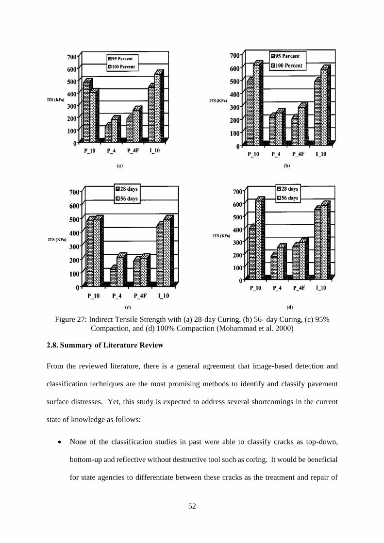
52
Figure 27: Indirect Tensile Strength with (a) 28-day Curing, (b) 56- day Curing, (c) 95%
Compaction, and (d) 100% Compaction (Mohammad et al. 2000)
Summary of Literature Review
From the reviewed literature, there is a general agreement that image-based detection and
classification techniques are the most promising methods to identify and classify pavement
surface distresses. Yet, this study is expected to address several shortcomings in the current
state of knowledge as follows:
None of the classification studies in past were able to classify cracks as top-down,
bottom-up and reflective without destructive tool such as coring. It would be beneficial
for state agencies to differentiate between these cracks as the treatment and repair of

53
these distresses is noticeably different. Therefore, the present study developed a novel
approach to differentiate between crack types based on the surface characteristics of
these cracks and pavement information.
Most of the previous studies have used complex image segmentation techniques in
crack identification and classification. These approaches of crack identification have
not been automated due to various complexities involved in pavement images such as
texture variability, poor background illumination and variations in roughness, intensity,
spots, stains, and road markings. Therefore, the present study developed a simple
automated approach for crack classification using simplified image processing
techniques.
None of the previous studies developed a deep learning model to classify the pavement
cracks into three classes as top-down, bottom-up, and CT reflective cracks. Hence, this
study developed a CNN model to classify the cracks into three classes.
None of the previous studies developed a tool that can be routinely used by PMS
engineers to classify the pavement surface cracks into top-down, bottom-up, and CT
reflective cracks. Therefore, this study developed a tool that can be used by
practitioners without advanced knowledge of machine-learning methods.
Most of the studies have used only the vertical contact pressures to calculate the
pavement responses. This study has incorporated both the vertical and tangential
contact pressures to calculate strain distribution at pavement layer interfaces.

54
METHODOLOGY
To achieve the objectives of the study, the research tasks were conducted into two phases. A
comprehensive literature review was conducted prior to undertaking the tasks in both phases
in order to gain more insights into the subject. The pertinent literature on top-down cracking,
Louisiana PMS, image-based crack identification methods, latest advancements in image-
based crack detection techniques, artificial neural network, finite element modeling of
pavement structure, and finite element analysis of top-down, bottom-up, and cement treated
reflective cracking were reviewed. In the first phase of study, CNN and ANN models were
developed for identification and image classification of cracks in flexible pavements. In the
second phase, finite element models were developed to simulate the loading conditions in the
field and to identify the stress mechanisms responsible for fatigue cracking, top-down cracking,
and cement treated reflective cracking in flexible pavements.
CNN and ANN Crack Classification Model
In-service flexible pavement sections were selected for analysis based on the parameters
identified for these sites. Images were acquired for in-service pavement sections exhibiting
top-down, bottom-up, and CT reflective cracking. These images were further processed to
include in the training, testing, and validation sets for the developed crack classification CNN
models. At once, design input variables namely pavement age, AC thickness, annual average
daily traffic (AADT), type of base, crack orientation, and crack location, were also collected
to use in the training, testing, and validation sets of the ANN-based decision making model.
The overall procedure is explained in details in the following sections.
3.1.1. PMS Data Collection
The images for analysis of the pavement cracks were obtained from the Louisiana Department
of Transportation and Development (LaDOTD) PMS inventory. The pavement network in

55
Louisiana is surveyed every two years using the ARAN system, which acquires continuous
high definition digital images of the pavement surface. The images for top-down cracking
were collected from PMS inventory based on the field verification of these cracks with coring.
The sections with potential top-down cracks were first identified based on the characteristics
of these cracks as suggested in the literature before cores were extracted for verification. To
collect the images with bottom-up fatigue and CT reflective cracks during the early
development phase, sections with typical bottom-up alligator cracks (fatigue) and CT reflective
cracks at specific locations were first identified using video surveys and were then projected
back to previous year’s survey for the same locations. Table 1 presents the total number of
cracking images collected for each cracking pattern.
Table 1: Image Data Collection for Each Crack Type
Crack Type Number of Control Sections Number of Images
Top-down cracking 9 162
Bottom-up cracking 10 66
CT reflective cracking 9 122
3.1.1.1 Pavement Sections Selection for Top-Down Cracking
The pavement sections with longitudinal cracks in the wheel path were selected as shown in
Figure 28. The design of the pavement and the time of rehabilitation/construction were the
main factors in selection of the pavement sections. Table 2 presents the pavement sections
used in the analysis.

56
Table 2: Pavement Sections Selected in the Analysis
Control
Section District Parish
Construction
Date Route
057-03 3 1 4/24/2015 LA 13
058-02 62 52 12/6/2012 LA 41
262-03 62 32 12/17/2013 LA 16
266-01 61 3 4/26/2013 LA 22
829-26 2 29 7/12/2013 LA 3235
857-63 3 57 5/28/2013 LA 82
015-05 58 30 10/15/2012 US 165
019-05 61 63 3/20/2012 US 61
030-04 62 59 11/1/2012 LA 21
(a)
Figure 28: Illustration of Pavement Section Selection for Top-Down Cracking, (a) iVision
Platform for Data Collection, (b) Pavement Image with Top-Down Cracking
(Fig. cont’d.)

57
(b)
3.1.1.2 Field Validation of the Sections for Top-Down Cracking
To validate the selected sections, field cores were extracted along the wheel path of the
pavement. The coordinates of the coring locations were extracted from the project maps in
PMS such that these locations correspond to the pavement images locations obtained from
PMS for image analysis. Figure 29 presents the acquisition process of field cores. The cores
were extracted at the tip of longitudinal crack in the wheel path to verify the top-down
orientation of the cracks.

58
(a) (b)
(c) (d)
Figure 29: Acquisition of Field Cores, (a) Marking Core Extraction Location, (b) Coring the
Marked Location, (c) Careful Extraction of Core, (d) Extracted Pavement Core
Field cores with longitudinal top-down cracking for two pavement sections are
presented in Figure 30. It is evident from the field cores that the crack started at the top of the
AC layer. Table 3 summarizes the cores obtained from the six pavement sections. Based on
field cores observation, the cracks were observed to extend up to a depth of 25 to 100 mm from
the pavement surface. The top-down propagation of the cracks was also confirmed in the field

59
with the drilled hole as some of the cores were fragmented during coring. Figure 31 presents
an illustration of the fragmented cores and the corresponding drilled hole.
(a) (b)
Figure 30: Cores Showing Longitudinal Top-down Cracks for Control Sections (a) 829-26,
(b) 857-63
Table 3: Summary of Coring
Control
Section/Route
AC Thickness
(mm)
Crack Depth
(mm)
Crack Width
(mm)
Vertical
Orientation
057-03 / LA 13 317.5 50 3 Top-down
058-02 / LA 41 203.2 25 3 Top-down
262-03 / LA 16 215.9 65 6 Top-down
266-01 / LA 22 355.6 50 4 Top-down
829-26 / LA 3235 203.2 95 3 Top-down
857-63 / LA 82 203.2 45 4 Top-down
Crack end
Crack end

60
Figure 31: Drilled Hole and Fragmented Core
3.1.1.3 Pavement Sections Selection for Bottom-up and Cement Treated Reflective Cracking
The sections selected for bottom-up and cement treated reflective cracking are presented in
Table 4 and Table 5, respectively. Figure 32 and Figure 33 present the procedure for the
selection of bottom-up and cement treated reflective cracking images from PMS. As shown in
Figure 32 and Figure 33, pavement sections with typical bottom-up and cement treated
reflective cracking were identified for year 2016. The locations of the cracks on these sections
were then projected back to previous years’ surveys until the crack initiation phase was
reached. The digital images for the year when crack initiated at the pavement surface were
then used to develop the models.
Crack end

61
Table 4: Pavement Sections with Bottom-up Cracking
Control
Section District Parish
Construction
Date Route
852-12 62 52 10/18/2001 LA 0434
034-03 8 43 10/28/2003 LA 0006
193-06 7 10 8/8/2007 LA 0014
262-02 62 32 N/A LA 0016
273-03 62 32 8/2/1996 LA 0064
391-02 3 28 12/20/1996 LA 0098
053-01 8 40 7/11/1996 LA 0001
414-02 61 24 7/19/1991 LA 0030
828-03 3 28 7/19/1995 LA 723
034-04 8 35 7/17/2003 LA 0006
Figure 32: Pavement Section Selection for Bottom-up Cracking

62
Table 5: Pavement Sections with Cement Treated Reflective Cracking
Control
Section District Parish
Construction
Date Route
014-06 8 40 5/8/2008 US 0165
015-02 8 40 6/4/2001 US 0165
048-01 4 9 8/25/2000 US 0079
054-05 7 27 7/18/2000 LA 0026
012-12 3 49 2/21/2013 US 0190
019-05 61 63 9/2/2003 US 0061
027-04 4 60 1/25/2006 US 0079
260-01 61 3 2001 LA 0042
273-03 62 32 1999 LA 0064
Figure 33: Pavement Section Selection for Cement Treated Reflective Cracking

63
3.1.2. Image Pre-Processing
The objective of this task was to process the pavement images obtained from the LaDOTD
PMS to enhance the cracks from the background and noise and use them in the training, testing,
and validation data sets in CNN. The image pre-processing technique involved five major
steps namely image acquisition, median filtering, morphological erosion, contrast
enhancement, and background subtraction as illustrated in Figure 34. The detailed description
of the image acquisition and processing techniques is presented in the following sections.
(a)
(b)
Figure 34: Illustration of Processed Input Images for (a) Top-down Cracking, (b) Bottom-up
Cracking, and (c) CT Reflective Cracking
(fig. cont’d.)
Original Image Median Filter Morphological
Erosion
Contrast
Enhancement Background
Subtraction

64
(c)
3.1.2.1. Image Acquisition
The objective of this step was to extract the pavement images from the LaDOTD PMS for the
sections presented in Table 4 and Table 5 and at the locations for which the cracks were
identified and were back-projected to the initiation phase.
3.1.2.2. Noise Reduction and Crack Enhancement
This step involves the visibility enhancement of particular features in the pavement images
with the application of specific enhancement and mathematical operations for 2D images. The
image pre-processing using different enhancement techniques intensifies cracks from random
backgrounds that include pavement surface texture, roughness, patches, spots, stains, raveling,
and road markings. The selection of appropriate filters is an important step in image pre-
processing in order to remove excessive noise while preserving the edges of the objects of
interest.
3.1.2.2.1. Crack Enhancement for 2D Images
The pavement noise reduction was achieved using a space-domain image filtering technique
known as a Median Filter (MF). This nonlinear filtering technique has been widely used in
pavement images as it has the advantage of removing background noise with low level of
blurring compared to mean filtering and Gaussian filter. The results of an application of 3x3

65
MF are presented in Figure 34. The image pixels of the original pavement images were
replaced with the median of its neighboring pixels while preserving the crack edges.
A morphological image processing technique known as gray scale erosion was applied for
further noise reduction and crack enhancement. The erosion of image I and the structuring
element S is defined as follows (Jahanshaho et al. 2009):
𝐼 ɵ 𝑆 = min [𝐼(𝑥 + 𝑥′, 𝑦 + 𝑦′) − 𝑆(𝑥′, 𝑦′) ∣ (𝑥′, 𝑦′) ∊ 𝐷𝑠 (3)
where,
Ds = the binary matrix;
S = the domain of structuring element, which defines which neighboring pixels are included in
the minimum function; and
I(x, y) is assumed to be +∞ for (x, y).
The best possible contrast distribution of pixel values was achieved using local contrast
enhancement. The image was then subjected to background subtraction, which removes gels
and shadows from the smooth continuous background. Figure 34 illustrates the overall noise
removal and image enhancement techniques employed for image data preparation of each crack
type.
3.1.2.2.2 Crack Enhancement for 2D and 3D Images
A CNN based crack classification tool was developed for a combination of both 2D and 3D
images. The similar approach for median filtering, morphological erosion, and contrast
enhancement as described in the previous section was applied for the combination of 2D and
3D images. However, before the application of aforementioned operations, the images were
first subjected to intensity normalization, which removes the non-uniform background in the

66
pavement images. The pixel intensity in a pavement image can be represented by the following
equation (Ying and Salari 2009):
𝑆(𝑝) = 𝑆𝑏(𝑝) + 𝑆(𝑝) + 𝑆𝑛(𝑝) (4)
Where, p is a pixel in a pavement image, Sb(p) is the intensity of the pixel, and , Sb(p), Sc(p),
and Sn(p) represent the background illumination signal, crack component signal, and signal due
to noise. The objective of this step is to arbitrarily normalize the background illumination
signal into a constant intensity value. The non-uniform background removal method proposed
by Ying and Salari was implemented with some modifications, which consisted of the
following steps (Ying and Salari 2009):
The image was partitioned into the rectangular windows of size 64*64.
For each window, the mean (Gmean), minimum (Gmin), and the maximum (Gmax) of the
gray level was calculated.
An upper (lu) and lower limit (ll) of gray intensity pixel was defined for each window.
The pixels outside these limits were considered as suspicious points for noise, cracks,
and other variations. A limiting factor of 50% was chosen for our images. The limiting
range was calculated using following equation.
𝑙𝑢 = 𝐺𝑚𝑒𝑎𝑛 + (𝐺𝑚𝑎𝑥 − 𝐺𝑚𝑒𝑎𝑛) ∗ 50% (5)
𝑙𝑙 = 𝐺𝑚𝑒𝑎𝑛 − (𝐺𝑚𝑎𝑥 − 𝐺𝑚𝑒𝑎𝑛) ∗ 50% (6)
An updated mean value (G’(mean)) was calculated for each window which represents
the mean for each window without considering the noise and crack pixels.
The background of each window was normalized by multiplying every point window
with a amplitude correction factor f which was calculated as, f = S/G’(mean), where S
is the target background value or the mean value of the original image.

67
The application of intensity normalization is illustrated in Figure 35.
Figure 35: Intensity Normalization
3.1.3. CNN Model
In this study, an image-based crack classification model was developed using deep learning
method through transfer learning and domain adaptation approach. The procedure involved
the use of the pre-trained CNN model known as AlexNet (Krizhevsky et al. 2012), which was
developed and trained based on a massive database containing millions of images as a feature
generator for pavement images. The pre-trained classifier was trained with labelled pavement
images to predict the pavement crack types (i.e., top-down, bottom-up, or cement treated
reflective cracking). The pavement cracks can be classified accordingly using a sliding
window and a CNN classifier that is generated through the training process (Li et al. 2019).
The developed model automatically generates the crack feature sets based on the input images
to classify the cracks into three categories.
Original Image Intensity
Normalization

68
3.1.3.1 AlexNet Architecture
The present study built a CNN model by modifying the AlexNet, which is a widely recognized
pre-trained CNN model for image classification. The architecture of the modified CNN
network is illustrated in Table 6 and Figure 36.
conv# = convolution, pool# = pooling, fc# = full connection
Figure 36: CNN’s Overall Architecture (Li et al. 2019)
The input sets consisted of 166, 66, and 122 pavement images with top-down, bottom-
up, and cement treated cracks, respectively. The patch size was set to 227 x 227 to save
computing time before feeding the CNNs with the training images. The first and second
convolution layers convolved the image matrix into 11 x 11 and 5 x 5 pixel sizes, respectively,
to obtain a better noise suspension while other convolution layers were equipped with kernel
of 3 x 3 and a stride of 1. The max pooling was performed in a filter size of 3 x 3 with a stride
of 2.
pool1 pool2
conv1 conv2 conv3 conv4 conv5 pool3
fc2
fc3 softmax
fc1

69
Table 6: Detailed Specifications of CNN Model
Layer Filter size Stride Padding Activations
conv1 11*11 [4 4] [0 0 0 0] 55*55*96
pool1 3*3 [2 2] [0 0 0 0] 27*27*96
conv2 5*5 [1 1] [2 2 2 2] 27*27*256
pool2 3*3 [2 2] [0 0 0 0] 13*13*256
conv3 3*3 [1 1] [1 1 1 1] 13*13*384
conv4 3*3 [1 1] [1 1 1 1] 13*13*384
conv5 3*3 [1 1] [1 1 1 1] 13*13*256
pool3 3*3 [2 2] [0 0 0 0] 6*6*256
fc1 - - - 1*1*4096
fc2 - - - 1*1*4096
fc3 - - - 1*1*1000
Softmax - - - 1*1*1000
Typical CNN models consist of convolutional layers, max pooling layers, and fully
connected layers. The modified network had 5 convolutional layers with 3 max-pooling layers
and 3 fully connected layers as shown in Figure 36. Table 6 presents the detailed specifications
of the different layers of the CNN model. The CNN architecture also included other operations
namely rectified linear units (ReLU), local response normalization (LRN), and dropout. The
ReLU is used as activation function after each convolution layer and the first two fully
connected layers; LRN is used before the first two pooling layers, and the dropout is used after
first two fully-connected layers. The softmax layer, consisting of three units for classification
of input data, was located at the end of the CNN’s structure. The overall architecture consisted
of 25 layers with 24 connections.
The objective function was optimized using stochastic gradient descent (SGD)
algorithm with momentum and ‘on-line’ or incremental training characteristic, which updates
the network parameter after each input during the training process. Through an iterative
procedure, SGD minimizes the loss function E(i) = D(D(i), F(W, Z(i))) which measures the

70
deviation of the true output ‘D’ for input ‘Z’ from output generated form CNN function F(W,
Z) (Li et al. 2018). The SGD was used with the initial learning rate of 0.01 and the momentum,
weight decay, and dropout rate were set to 0.9, 0.0001, and 0.5, respectively. The classifiers
were trained for 8 epochs with a batch size of 25.
3.1.4. ANN Decision-Making Tool
3.1.4.1. Pattern Recognition System
A decision-making tool was developed using ANN to serve as a secondary screening tool and
to cross-validate the image-based classification results obtained from the CNN model. The
tool used input variables related to pavement conditions and crack properties and was
developed using ANN-based pattern recognition system. This was achieved by using a
multilayered feed forward ANN with a hard-lim transfer function that presents the output as
‘0’ or ‘1’. A scaled conjugate gradient back-propagation algorithm (trainscg) was used for the
network optimization. The confusion matrices having two dimensions, one with the actual
class of the input and other with the predicted class, were used to express the accuracy of the
system. Figure 37 presents a basic confusion matrix with patterns P1, P2, and Pn. The Nij
represents the number of samples actually belonging to class Pi but classified by the ANN as
class Pj (Deng et al. 2016). The tool can be used separately or in conjunction with the CNN
model to cross-validate the predicted crack type obtained from the image-based CNN model.

71
Predicted
P1 … Pj … Pn
Act
ual
P1 N11 N1j N1n
⁞
Pi
⁞
Ni1
⁞
… Nij …
⁞
Nin
Pn Nn1 Nnj Nnn
Figure 37: Confusion Matrix for Pattern Recognition ANN (Deng et al. 2016)
3.1.4.2 Network Inputs and ANN Structure
The input layer was fed with simplest set of inputs corresponding to the images and that
required no optimization analysis to be conducted. The input set consisted of six different
variables including pavement age, base type, AADT, AC thickness, orientation of cracks, and
location of cracks, which are readily available from the LaDOTD PMS. Each input was divided
into different classes and was assigned a numerical value. Figure 38 presents the classification
and numerical values assigned to each input; the numbers in front of each class represent the
assigned numerical value. Figure 39 presents the ANN structure. As shown in Figure 38, six
ANN consisted of six neurons in the input layer to incorporate six different inputs and the target
layer comprised of three neurons to incorporate the corresponding prediction classes. The
adequate correlations between the inputs and targets were established with a hidden layer
consisting of ten neurons by connecting to each neuron in the input and target layers. An
iterative process was used to select the number of neurons in the hidden layer such that the
least number of hidden neurons are selected without affecting the network performance.

72
Figure 38: Inputs for ANN Model
Figure 39: ANN-based Pattern Recognition Model Structure
Finite Element Modeling
3.2.1. Model Formulation
The commercial software ABAQUS CAE 6.13 was used for FE modeling of flexible
pavements. Figure 40 presents the general layout of the developed FE models. The three
dimensional symmetrical models have been constructed as a combination of pavement layers
and surrounding ground. Three models were constructed to simulate low volume, medium
volume, and high volume traffic for flexible pavements. The thickness of wearing course,
binder course, base layer, and sub-base course used in the flexible pavements simulation is
Inputs
Pavement Age (years)
1. 0-5
2. 6-12
3. 13+
AC Thickness
(in.)
1. 0-5
2. 5.5-13
3. 13.5+
Base Type
1. Cement Treated
2. Untreated
3. PCC
AADT
1. 0-5000
2. 5001-10000
3. 10001+
Crack Orientation
1. Longitudinal
2. Transverse
3. Longitudinal and Transverse
Crack Location
1. Wheel Path (if
Longitudinal)
2. Outside Wheel Path (if Longitudinal
3. If orientation is transverse or
longitudinal and transverse

73
presented in Table 7. The dimensions of the developed models (i.e. 1304mm x 1900mm) were
selected such that any edge-effect errors would be minimized and elements’ sizes are retained
within the acceptable limits.
Table 7: Layer Thickness for Flexible Pavements
Traffic
Asphaltic concrete (mm)
Sub-base Course (mm) Wearing course Binder course Base course
Low 38 50.8 NA 216
Medium 50.8 101.6 NA 216
High 50.8 101.6 152.4 216
Figure 40: General Layout of FE Model
3.2.2. Step and Increment
Two analysis steps namely static and visco were defined to generate two stages in the
simulation for flexible pavement analysis. The static step allows the vertical pressure to act
upon the starting zone and avoid the influence of oscillation and energy waves. Then, a visco

74
step is constructed to perform a quasi-static nonlinear analysis. The increment divides the total
time period of the visco step based on the vehicle speed and can be defined based on fixed time
incrementation or calculated by ABAQUS automatically. The incrementation of the visco step
was fixed with the maximum number of increments set at 100.
3.2.3. Finite Element Mesh
A relatively fine mesh was generated around the load to give an optimal accuracy to the model.
The C3D8R elements, which are 8-node linear brick elements with reduced integration (1
integration point) were used to improve the rate of convergence and to reduce calculation time
and the thickness of the elements were varied, depending on the layers. The integration point
of these elements are located in the middle of the element, requiring small elements to capture
a stress concentration at the boundary of the structure. These elements use linear interpolation
in each direction and are often called as linear elements or first-order elements. Figure 41
presents the general mesh of the FE model.
Figure 41: General Mesh of the FE Model
Pavement
Layers
Symmetric
Area
Surrounding
Ground
Loading Area

75
All layers were partitioned with the same shape to avoid any contact interaction
complexity between the consecutive layers. The total number of elements varied with the
different pavement types in the analysis. The structure was meshed with lager element size on
the surrounding and smaller elements near the tire pavement contact zone to obtain accurate
solution and to reduce calculation time. The completed job did not include any warning or
error indicating that the solution was sufficiently accurate.
3.2.4. Load and Boundary Conditions
A dual tire assembly was considered to simulate the vehicular loading. In contrast to the
layered theory, which assumes a circular area of load application, the developed FE model
incorporated the exact geometry of the loading area and the appropriate pressure conditions on
each tire tread. The loading modeled as a set of time interval vertical pressures and the
boundary conditions are presented in Figure 42. The model boundary in X and Y coordinates
was restrained to displacement and rotation in all directions; which signifies that all degrees of
freedom at the boundary nodes are equal to zero. The rigid boundary condition reflects the
energy waves completely.
Figure 42: Pavement Load Contact Area and Boundary Conditions
Contact
Area
Boundary
Conditions

76
The dimensions and shape of the tire assembly are presented in Figure 43. The
dimensions and shapes of dual tire was obtained from the manufacture after one of the tire
pressures was tested at the Virginia Smart Road at a nominal pressure of 720 kPa (Al-Qadi et
al. 2005). Rectangular contact areas were defined to accurately simulate the tire movement
over the pavement surface. The actual contact area assumes a rectangular shape with a constant
ratio between the width and length (Huang 1993).
(a)
(b)
Figure 43: (a) Tire Footprint of Dual Tire Assembly; (b) Modeled Contact Area for Dual-Tire
Assembly (Al-Qadi et al. 2005)
The movement of the tire was simulated by assuming the quasi static approach, where
the loading area and amplitude are gradually shifted over the fine mesh of the loading track.
The movement of the tire over the entire length of model was achieved by 21 increments of the
532 kPa
766 kPa867 kPa
766 kPa
532 kPa
36mm
34mm 34mm 34mm
36mm

77
load, with the load moved a 40-mm distance in each increment. Table 8 presents the stresses
and tire dimensions at the nominal tire inflation pressure of 720 kPa. As shown in Table 8, the
transverse shear stresses at the tire ribs are high by as much as 52% while the longitudinal shear
stresses are less than 10% of the vertical stresses.
Table 8: Tire Dimensions and Maximum Stresses at Different Tire Ribs.
R1 G1 R2 G2 R3 G3 R4 G4 R5
Length (mm) 160 - 200 - 200 - 200 - 160
Width (mm) 36 10 34 10 34 10 34 10 36
Vertical Shear Stress (kPa) 532 - 766 - 867 - 766 - 532
Transverse Shear Stress (kPa) 277 - 207 - 182 - 184 - 277
Longitudinal Shear Stress (kPa) 46 - 60 - 70 - 57 - 42
*R: Tire rib, G*: Tire groove between two ribs
The subgrade’s stiffness effects and support to the pavement structure was simulated by using
elastic element foundations, which act as springs to the grounds. The modulus of the subgrade
reaction was assumed to be 175 N/cm3, which corresponds to a medium stiffness of the
subgrade. Full bonding interaction with small sliding was assigned between the pavement
layers with node to surface discretization. The typical amplitude-time curve used for the
movement of the load is presented in Figure 44.
Amplitude 1 Amplitude 2
Ts
Figure 44: Amplitudes on Contact Area
Am
pli
tude
Time
Te

78
The duration of Amplitude is Te – Ts, where Ts and Te represent the starting and
overlapping time for the amplitude. This duration of amplitude varies with the vehicular speed.
For example, for a vehicle speed of 9 mph (4000 mm/s), with the load moving 40 mm in each
increment, the time used by the tire passing the elements is 0.01 seconds.
3.2.4.1 Shrinkage Modelling
The shrinkage in cement treated base (CTB) was modeled using displacement boundary
conditions. The shrinkage strains in CTB with time was obtained from the literature and is
shown in Figure 45 (Cho et al. 2006). Figure 45 illustrates the shrinkage in CTB with time.
These strains at each time period were converted to corresponding displacement and were used
as a displacement boundary condition at each step of the analysis. These displacements were
applied on the Y-axis of the CTB layer while restraining other directions from movement.
Figure 45: Shrinkage Strain at CTB with Time (Cho et al. 2006)
-450
-400
-350
-300
-250
-200
-150
-100
-50
0
0 5 10 15 20 25 30 35 40 45 50
Shri
nkag
e (m
icro
stra
in)
Time (days)
Shrinkage at CTB

79
3.2.4.2 Material Characterization
Viscoelastic constitutive model was used to simulate the behavior of the AC layers and elastic
constitutive model was used to simulate the granular and subgrade layers. The elastic
properties of the granular materials and the subgrade were derived from the results of the model
validation where the measured and calculated stress and strains at the bottom of the AC layer
were compared. The viscoelastic properties of the AC layer were obtained from the results of
laboratory testing in the extracted cores (Elseifi et al. 2012).
Characterization of the viscoelastic properties of AC surface mixes was performed
using the Asphalt Mixture Performance Tester (AMPT) in accordance to AASHTO TP-79.
The dynamic modulus testing was conducted at five temperatures (-10, 5, 25, and 37.8, and
54°C) and six frequencies (0.1, 0.5, 1, 5, 10, and 25 Hz). The dynamic modulus data from the
test were shifted to a reference temperature of 25°C using a sigmoidal function in order to
construct a master curve. The isotropic linear viscoelastic behavior of AC was described using
a generalized Maxwell model, which consists of a spring and n Maxwell elements connected
in parallel (Al- Qadi et al. 2008):
G (t) = G0 + ∑ gi(1 − e−t
τi⁄ )N
i=1 (7)
where,
G (t) = shear relaxation modulus at time t;
gi = material constants; and
i = retardation times.
To fit the Maxwell equation to the sigmoidal model, a built-in module in the FE commercial
software ABAQUS was used. A nonlinear least squares curve fitting process was used to fit
the variations of the normalized shear modulus with time. The viscoelastic properties of the
AC layer were defined at 25°C after an accurate fit was obtained using 11 to 13 Prony series.

80
3.2.5. Model Validation
The results from the FE model were compared with actual stress and strain measurements at
the Louisiana Accelerated Loading Facility (ALF). This was an essential step in the analysis
such that the various parameters in the FE model can be calibrated, so as to arrive to the best
simulating assumptions to represent the field conditions. Although the analytical solution
allows better variation of the parameters, the effectiveness of various aspects of the finite
element approach such as boundary conditions, interaction properties, and mesh can only be
truly validated by comparing with field measurements. Based on the available laboratory
results and modeling limitations, the developed FE models were validated with some
approximations to approach field pavement conditions.
3.2.5.1 Accelerated Loading Facility
The Louisiana Accelerated Loading Facility (ALF) is a comprehensive loading facility with a
moving load assembly that can simulate the effect of traffic loading on pavement by applying
a controlled repetitive load (King and Abadie 1999). Figure 46 presents the ALF at Louisiana
(Wu et al. 2012).
Figure 46: The Louisiana Accelerated Loading Facility (Wu et al. 2012)

81
The constant truck wheel load is applied by a loading wheel that travels at a speed of
about 4.5 m/s (10 mph) to a loading length of 26 m with approximately 10 m of constant
velocity loading of the wheel. The ALF facility can apply approximately 380 load cycles per
hour and the loads can be varied from dead weight of 43.4kN (9750 pounds) to 94.5kN (21,250
pounds) by adding static load plates.
3.2.5.2 Test Section
This research project utilized the results of Experiment III, which was designed and constructed
to evaluate the performance of Reclaimed Asphalt Pavement (RAP) used as an aggregate
interlayer between the cement-treated base and asphalt concrete layers (Mohammad et al.,
2008). The test lane, 66 m x 4 m, consisted of a RAP interlayer used in base layer on top of a
254 mm (10 in.) cement stabilized subgrade layer. The pavement design and instrument plan
for the test lane is presented in Figure 47. The strain gauge and pressure cells were embedded
to the pavement during construction. The load was applied using a dual tire configuration at a
pressure of 0.7 MPa (105 psi) and at a constant speed of 4.5 m/s. Table 9 presents the input
parameters for ALF test section.
Plan View Section View Legend
Figure 47: Pavement Design and Instrumentation Plan in Experiment III (Elseifi 2009)
88.9 mm AC
88.9 mm RAP
254 mm Soil Cement (5%
Cement)
Subgrade Pressure Cell - Rt
Subgrade Pressure Cell - Lt
Sub-base Strain Gage - Rt
Sub-base Strain Gage - Lt
Base Pressure Cell - Rt
Base Strain Gage - Rt
Base Strain Gage - Lt
381 mm 381 mm
381 mm
190
mm
190
mm

82
Table 9: Input Parameters for ALF Test Section Obtained from Model Validation
Pavement Layer Elastic Modulus (MPa) Poisson's ratio
AC 8000 0.3
RAP Interlayer 2000 0.3
Base (Soil-Cement) 3300 0.35
3.2.5.3 Testing Procedure and Instrument Response
The test lanes were loaded continuously at a pressure of 0.7 MPa with a dual 11R22.5 radial
ply truck tire moving at a constant speed of 4.5 m/s. Nearly 2.3 x 10⁶ Single Axle Loads
(ESALs) were applied over the loading process of two years and eight months. To minimize
the environmental effects and seasonal variation between the test lanes, the loading was applied
alternatively between the test lanes in 25,000 pass increments. Figure 48 presents a typical
strain signals measured at the bottom of surface layer (88.9 mm) after 25,060 passes; the
response was compressive at the beginning, then tension, and compressive again. The strain
measurements were observed to be consistent until approximately 350,000 passes. Figure 49
presents the stress response at a depth of 88.9 mm (3.5 in.); the compressive stress was mostly
measured in the vertical direction.
Figure 48: Measured Longitudinal Strain at the Bottom of Surface Layer after 25,060 Passes
(Elseifi 2009)
-30.00
-20.00
-10.00
0.00
10.00
20.00
30.00
40.00
0.00 0.50 1.00 1.50 2.00 2.50 3.00
S
t
r
a
i
n
Time, sec

83
Figure 49: Measured Vertical Stress at the Bottom of Surface Layer after 47,505 Passes
(Elseifi 2009)
3.2.5.4 Calculated and Measured Responses
The FE model was validated using the stress and strain results at bottom of the AC layer. The
stress and strain results at lower repetition of load were used to validate the model. Figure 50
and Figure 51 illustrate the comparison of calculated and measured stress and strain responses
due to a dual tire assembly moving at a speed of 4.5 m/s (10mph). As shown in the figure, a
good agreement was observed between the results of the FE model and the responses of the
strain gauge and pressure cell. Similar to the measured response, the strain from the FE model
was observed to be compressive at the beginning, then tension and compressive again, and the
stress was compressive in the vertical direction. The root mean square error (RMSE) was
computed to be 2.97% and 3.86% between the measured and calculated stress and strains,
respectively. Based on these findings, it may be concluded that the developed FE model is
capable of predicting pavement responses to vehicular loading.
-5.00
0.00
5.00
10.00
15.00
20.00
25.00
30.00
35.00
40.00
0.00 2.00 4.00 6.00 8.00 10.00 12.00 14.00
S
t
r
e
s
s
Time, sec

84
Figure 50: Measured and Calculated Longitudinal Strains at the Bottom of AC Layer
Figure 51: Measured and Calculated Vertical Stress at the Bottom of AC Layer
-10
-5
0
5
10
15
20
25
30
35
40
0.01 0.06 0.11 0.16 0.21 0.26 0.31 0.36 0.41 0.46 0.51
Mic
rost
rain
Time (Sec)
Measured Calculated
-0.05
0
0.05
0.1
0.15
0.2
0.25
0.3
0.35
0 0.1 0.2 0.3 0.4 0.5 0.6
Str
ess
(MP
a)
Time
Measured Calculated

85
DEVELOPMENT AND VALIDATION OF CNN AND ANN
MODELS
This chapter provides the results of a CNN image classification tool that utilize digital
pavement images to classify pavement cracking. This chapter also provides the results of ANN
decision making tool that may assist the users to cross validate the CNN based classification.
CNN Network Performance
The data processing, CNN training, testing, and validation were performed in MATLAB 2019a
platform in a computer with Intel Core i5-4590S microprocessor and 8GB of RAM. A data set
consisting of 200 2D pavement images of size about 2500 x 4000 and 150 3D images of size
approximately 1030 x 1610 were collected from the LaDOTD PMS database. These images
were pre-processed using an automated preprocessing tool consisting of the aforementioned
image processing steps. The data were then divided into 60% for training, 15% for testing, and
25% for validation. The accuracy of the model was expressed in form of confusion matrices,
which present the actual and predicted crack types in terms of number and percentage.
The developed CNN model was trained, tested, and validated for two data sets: a data
set consisting of 2D images only and a data set consisting of both 2D and 3D images. Figure
52 presents the accuracy of CNN model for the raw pavement images. As shown in Figure 52,
the model achieved an accuracy of 61.7% and 73.4% on testing and validation phases,
respectively. The models accuracy for raw images is due to different factors such as pavement
noise, background illumination, pavement marking, spots and stains including cracking pattern.
The pavement images in two data sets were then processed with different image processing
techniques. For the data set consisting of 2D images only, the developed network achieved an
overall accuracy of 88.9% and 86.7% in the testing and validation phases, respectively. Figure
53 presents the confusion matrices for testing and validation. Similarly, for the data set
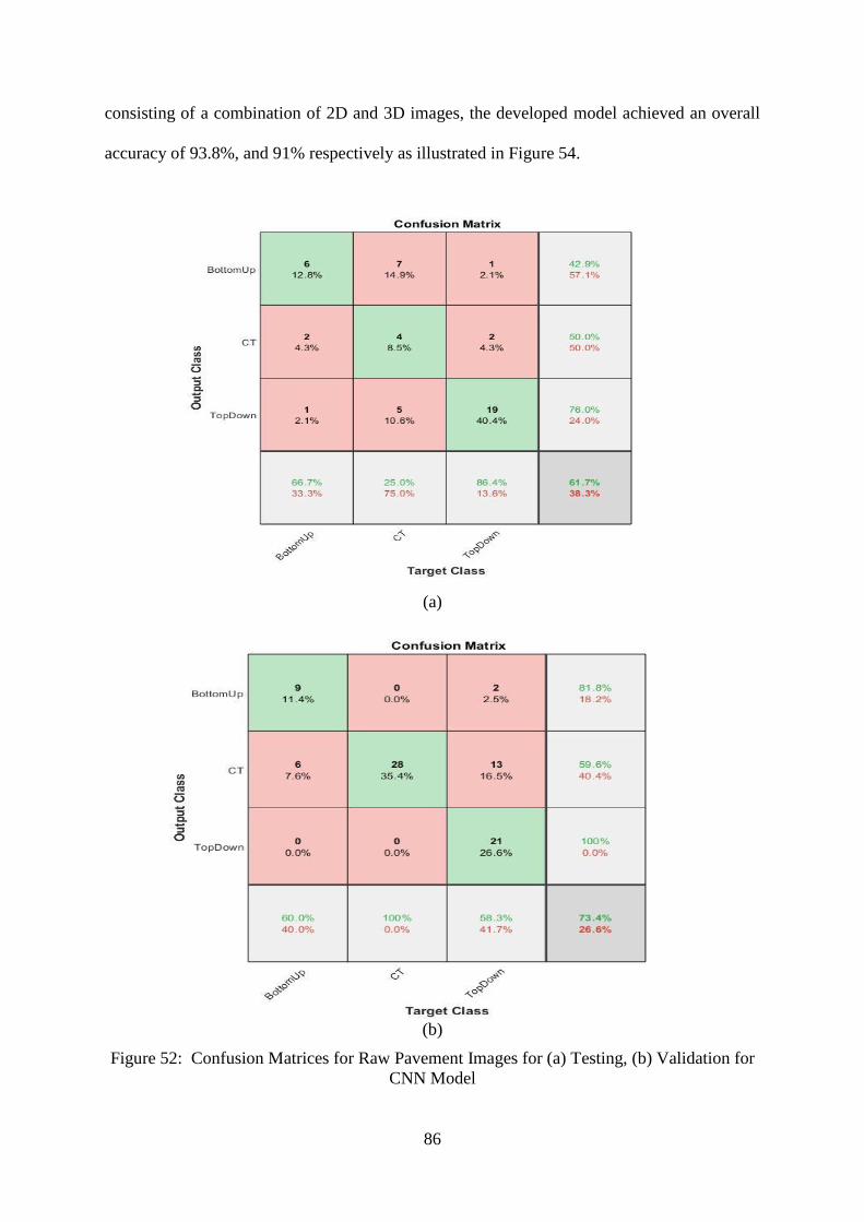
86
consisting of a combination of 2D and 3D images, the developed model achieved an overall
accuracy of 93.8%, and 91% respectively as illustrated in Figure 54.
(a)
(b)
Figure 52: Confusion Matrices for Raw Pavement Images for (a) Testing, (b) Validation for
CNN Model

87
(a)
(b)
Figure 53: Confusion Matrices for 2D Images for (a) Testing, (b) Validation for CNN Model

88
(a)
(b)
Figure 54: Confusion Matrices for 2D and 3D Images for (a) Testing, (b) Validation for
CNN Model

89
The dropout layers after the first two fully connected layers reduced the data overfitting
by preventing complex co-adaptations during network training. The dropout layer randomly
ignores some hidden and visible neurons during training and prevents the co-dependency
amongst the neurons. However, the dropout layer requires additional computational expense
for model training. In order to enhance the convergence and calculation speed, ReLU layers
were connected to the convolutional and fully connected layers. The ReLU layers implements
the activation function and determines the output of the neural network. The output of ReLU
layers was generalized using the LRN which implements the lateral inhibition in order to
reduce the capacity of a neuron that impedes the activity of its neighbors.
ANN Training and Performance
A computational tool available in MATLAB 2019a was used to process all the data and to
develop the decision-making ANN tool. The input data corresponding to 150 pavement images
used in the ANN model were collected from the Louisiana PMS. The data were then divided
into 70%, 15%, and 15% for training, validation, and testing respectively. Data overfitting was
avoided by halting the training process when the validation set error stopped decreasing. The
testing data was used to provide independent measure of the network performance as it had no
effect on the training. As shown in the figure, the ANN tool achieved an accuracy of 91.3%
in the testing and validation sets. Figure 55 presents the confusion matrices for training,
validation, testing, and overall step for pattern recognition system. The confusion matrices
showed an overall prediction accuracy of 92% indicating the effectiveness of the ANN model
to predict crack types in the evaluation process.
The generalization ability of the overall network was enhanced and overfitting was
avoided by halting the training as there was no observed decrease in the validation set error as
shown in Figure 56. The matrices present Nij with corresponding percentage, precision of every

90
decision, and overall accuracy as discussed in Chapter 3. The testing data set was used to
provide an independent measure of the network performance. The network training time was
found to be 4.2 seconds.
Where, 1 = bottom up cracking, 2 = cement treated reflective cracking, and 3 = top down cracking
Figure 55: Confusion Matrices for the Pattern Recognition System for Training, Validation,
and Testing for ANN Model

91
Figure 56: ANN Model Performance
Forward Calculations
The trained and validated CNN and ANN models were used to perform forward calculations
and to predict the crack type with an independent set of images and variables. The CNN and
ANN models can be saved as a MATLAB file once the desired accuracy is achieved in training
and validation phases, which later can be used to perform forward calculations for crack
classification. The data set consisting of 12 images with top-down cracking, 11 images with
bottom-up cracking, and 8 images with cement treated reflective cracking and their respective
pavement and crack characteristics was collected to assess the accuracy of the developed
models. Table 10 presents the results of the forward calculations.
Table 10: Forward Calculation Results
Crack Type
Number
of Test
Images
Correctly
Predicted
by CNN
Correctly
Predicted by
ANN
Correctly Predicted by
both CNN and ANN
Top-down 12 11 (91.7%) 12 (100%) 11 (91.7%)
Bottom-up 11 10 (90.1%) 10 (90.1%) 10 (90.1%)
CT reflective 8 7 (87.5%) 7 (100%) 7 (87.5%)
Total 32 28 (87.5%) 29 (90.6 %) 28 (87.5%)

92
As shown in Table 10, both CNN and ANN models achieved a satisfactory accuracy in
crack classification. The CNN and ANN models in MATLAB were subsequently incorporated
into a user-friendly computer program, which can be used by PMS engineers without advanced
knowledge of machine-learning techniques. Based on the results of forward calculations, the
following observations are made.
The CNN model accurately predicts the crack types for all images with distinct cracks.
However, for the images with poor background illumination, excessive shadows, spots
and stains, and containing blurry cracks, the crack classification should be validated
with the predicted crack type from the ANN-based model.
The prediction accuracy of top-down cracks for both models was higher compared to
bottom-up and CT reflective cracks; this can be attributed mainly to three distinct
characteristics of top-down cracks (crack orientation, crack location, and pavement
age). Compared to the ANN model, the CNN model more accurately predicted the
crack types for pavements that developed top-down cracks at later stages in their service
life.
The bottom-up cracking usually appear in the surface during the later stages of
pavement service life. However, for the pavements with relatively small AC thickness
and high traffic volume, the bottom-up cracks were observed to resemble top-down
cracking. In this case, the models’ accuracy was slightly inferior to other cases.
The CT reflective cracks usually initiate as transverse and longitudinal cracks in the
pavement with cement treated base and can appear during early or later stages of
pavement service life. The CT cracks that appeared only as longitudinal crack in the
wheel path were mistakenly classified as top-down or bottom-up cracking by the CNN
model. Therefore, the crack classification should be cross-checked with the predicted
crack type from the ANN-based model.

93
FINITE ELEMENT RESULTS
The finite element models were developed as a part of the study to identify the specific stresses
and locations of fatigue and cement treated reflective cracking in flexible pavements. To
identify the specific stresses responsible for cracking, the effect of (i) vertical stress and (ii)
vertical stress with tangential stresses on the tensile strains at the surface and bottom of the AC
layer were studied for pavement structures suitable for low, medium, and high traffic volumes.
To identify the critical locations of the cracks, the strains were obtained at different locations
in the pavement layers including underneath the tires and away from them. The stresses
associated with shrinkage in the cement-treated layer were investigated as the major cause of
cement-treated reflective cracking in semi-rigid pavements.
Effect of Tangential Stresses on Tensile Strain
The transverse and longitudinal shear stresses were incorporated into the finite element models
to study the effect of tangential stresses in the tensile strains at the pavement surface and at the
bottom of the AC layer. Pavement responses at various depths due to vertical tire loading were
first computed and were compared with the response due to combined vertical and tangential
loadings. Figure 57 presents the comparative analysis of the effect of tangential stresses on
the tensile strains at the surface and at the bottom of AC layer. As shown in the figure,
transverse stress due to tire loading significantly affected the tensile strains at the tire-pavement
contact surfaces. The tensile strains at the pavement surface were observed to increase by
approximately 68%, 63%, and 53% respectively for low, medium, and high volume flexible
pavements indicating an increased potential for the initiation and development of top-down
cracking when tangential stresses are considered in the analysis. The literature suggests that
this effect could be more pronounced with the increase in temperature. The incorporation of
transverse stress at pavement surface marginally increased the tensile strains at bottom of the

94
AC layer by approximately 7%, 6%, and 3% respectively for low, medium, and high volume
flexible pavements.
The longitudinal shear stress on the other hand was observed to have minimal effect on
the tensile strain at the pavement surface; this effect was also negligible at the bottom of AC
layer. The tensile strains at pavement surface were observed to increase by less than 5% for
all pavements with the incorporation of the longitudinal shear stresses. The combined effect
of transverse and longitudinal stresses on tensile strains at bottom of asphalt layer was observed
to be minimal suggesting that the surface shear stresses have lower impact on bottom-up fatigue
crack initiation. Results also indicated that flexible pavements used for low traffic volume had
a higher probability of developing fatigue cracking as they exhibited higher tensile strains.
Figure 57: Tensile Strains at Pavement Surface and Bottom of AC Layer due to Vertical and
Tangential Stresses
Low
Volume
Medium
Volume
High
Volume
Low
Volume
Medium
Volume
High
Volume
Surface Bottom of HMA
With Vertical Stress 152.07 132.11 131.18 343.35 255.94 217.20
With Transverse Stress 255.03 215.98 201.13 366.51 270.38 223.99
With Longitudinal Stress 266.118 224.286 207.314 367.42 270.92 224.31
0.00
50.00
100.00
150.00
200.00
250.00
300.00
350.00
400.00
Ten
sile
Str
ain (
μ)
With Vertical Stress With Transverse Stress With Longitudinal Stress

95
Critical Locations of Crack Initiation
The horizontal strain distributions at the pavement surface and at bottom of the AC layer due
to vertical and tangential stresses are presented in Figure 58. The tensile strains were obtained
at mid-point of the dual tire assembly, center of each tires, edges of the tires, and at distance of
125 mm and 250 mm away from the tires. As shown in the figure, the highest tensile strain
occurred underneath the center of each tire, which is reasoned to be the cause of the appearance
of fatigue cracking in the wheel path.
(a)
Figure 58: Tensile Strain Distribution at (a) Asphalt Surface, (b) Bottom of AC Layer
(fig. cont’d.)
-50
0
50
100
150
200
250
300
-600 -400 -200 0 200 400 600
Ten
sile
Str
ain (
μ)
Distance from Tire Center (mm)
Low volume (with tangential stress) Medium volume (with tangential stress)
High volume (with tangential stress) Low volume (without tangential stress)
Medium volume (without tangential stress) High volume (without tangential stress)

96
(b)
Shrinkage Effect on Tensile Stress
The drying shrinkage of cement treated base is the major factor that causes shrinkage cracking
in cement treated base. The cracks initiate when the tensile stresses due to shrinkage exceed
the tensile strength of the paving material. Figure 59 presents the tensile stresses at the cement
treated base for laboratory measured shrinkage strains presented in Figure 45 (Cho et al. 2006).
The indirect tensile strength (ITS) of cement treated base vary with the cement content,
aggregate percentage in the mix, and degree of compaction (Xuan et al. 2012). Studies have
reported that the ITS of CTB to be around 0.27 MPa at 7 days of curing and 0.62 MPa at 56
days of curing (Xuan et al. 2012, Mohammad et al. 2000). As shown in Figure 59, the tensile
stresses due to shrinkage at CTB is approximately similar to the tensile strength of the material
at 7 days. It can be inferred from the chart that the tensile stress at CTB will be higher than
0
50
100
150
200
250
300
350
400
-600 -400 -200 0 200 400 600
Ten
sile
Str
ain (
μ)
Distance from Tire Center (mm)
Low volume (with tangential stress) Medium volume (with tangential stress)
High volume (with tangential stress) Low volume (without tangential stress)
Medium volume (without tangential stress) High volume (without tangential stress)

97
tensile strength of material at 56 days indicating the shrinkage cracks to initiate within few
weeks after construction.
The tensile strength of asphalt concrete is dependent upon various parameters including
binder type and content, aggregate type, air void content, and aging. The indirect tensile
strength (ITS) of AC may vary from 0.62 Mpa to 1.4 MPa as reported by different studies (Kim
et al. 2012, Preciado et al. 2017, Taherkhani and Arshadi, 2019, Xiao 2009). Based on the
literature, a typical value of 1.03 MPa was adopted for this study. As shown in Figure 59, the
induced tensile stresses at bottom of asphalt layer due to shrinkage in CTB are comparable with
the tensile strength of AC. These stresses increase as the cracks become wider causing the
cracks to reflect in AC layer and appear as cement treated reflective cracking in pavement
surface.
Figure 59: Tensile Stresses due to Shrinkage
-1.2
-1
-0.8
-0.6
-0.4
-0.2
0
0 10 20 30 40 50 60
Ten
sile
Str
ess
(MP
a)
Time (Days)
Tensile stress (Asphalt bottom) Tenisle stress (At CTB)
Tensile strength at 7 days Tensile strength at 56 days
Tensile strength of AC

98
Parametric Studies
5.4.1. Effect of AC Layer Thickness on Tensile Strain
The effect of AC layer thicknesses on the tensile strains at the pavement surface and at the
bottom of the AC layer was studied for the medium traffic volume pavement design. The effect
of tangential shear stresses were also studied for four different thicknesses (1.5 in., 3.5 in., 5.5
in., and 8 in.) of AC layer for a pavement structure typically used for medium volume traffic.
The tensile strain at the pavement surface was observed to decrease with the increase in AC
layer thickness. In addition, the average increase in tensile strain at the pavement surface with
the incorporation of tangential stresses was approximately 60% for all pavements. In contrast,
the tensile strain at the bottom of AC layer increased by approximately 9% for pavement with
38mm (1.5 in.) AC layer with the incorporation of tangential loading while the increase was
only 1.5% for pavement with 203.2mm (8 in.) thick AC. The results of parametric study for
the AC layer thickness are presented in Figure 60.
Figure 60: Effect of Asphalt Concrete Layer Thickness on Tensile Strain
1.5 in. 3.5 in. 5.5 in. 8 in. 1.5 in. 3.5 in. 5.5 in. 8 in.
Surface Bottom of HMA
Without Tangential Stress 191.96 162.81 132.11 94.18 533.39 348.54 255.94 197.103
With Tangential Stress 308.48 258.65 215.98 156.37 581.00 372.87 270.38 200.495
0
100
200
300
400
500
600
700
Ten
sile
Str
ain (
μ)
Asphalt Concrete Thickness

99
5.4.2. Effect of Surface Mix Type on Tensile Strain
The maximum tensile strains at the surface and at the bottom of the AC layer was computed
for five different surface mixes to study the effect of the stiffness of the asphalt layer on the
cracking potential of flexible pavements. Table 11 presents the description of the surface mix
types used in the analysis. The tangential shear stresses were considered while computing the
maximum horizontal tensile strains. Figure 61 presents the results of the parametric study.
Table 11: Description of the Evaluated Mixes (Elseifi et al. 2012)
Mixture Abbreviation Description
64CO Conventional AC mixture with PG 64-22
70CO Conventional AC mixture with Styrene-Butadiene Styrene
Polymer-Modified PG 70-22
76CO Conventional AC mixture with Styrene-Butadiene Styrene
Polymer-Modified PG 76-22
76RAP15 AC mixture with Styrene-Butadiene Styrene Polymer
Modified PG 76-22 and 15% RAP
64RAP40 AC mixture with PG 64-22 AC containing 40% RAP and
engineering additives
Figure 61: Effect of Surface Mix Type on Tensile Strains at Pavement Surfaces
0
50
100
150
200
250
300
350
64RAP40 76RAP15 76CO 64CO 70CO
Ten
sile
Str
ain (
μ)
Surface Mixes
Bottom of HMA Surface
100
As shown in Figure 61, the horizontal tensile strains were lower for mixes with
reclaimed asphalt pavement (RAP) compared to the conventional mixes. The increased
stiffness of the RAP mixes offered more resistance to the vertical and tangential loading at the
pavement surface, thus reducing top-down cracking potential. However, one should
acknowledge that the presented analysis did not consider the strain and deformation tolerances
of the mixes, which would be lower for asphalt mixes with RAP materials than for asphalt
mixes with virgin materials.
5.4.3. Effect of Fly Ash and Admixtures on Tensile Stress Distribution
Cho et al. (2006) studied the effect of fly ash and varying percentage of expansive additives
and shrinkage reducing agent on shrinkage of the test specimen and observed that the shrinkage
reduced by as much as 48% at 48 days when 25% fly ash was added to the mix. The addition
of fly ash with shrinkage reducing agents reduced the shrinkage by only 25% to 40%. The
results of the experiments were previously presented in Figure 24. A parametric study was
conducted to observe the effect of drying shrinkage due to the addition of fly ash and fly ash
with admixtures and shrinkage reducing agents on the tensile stresses in the CTB (see Figure
62).
The addition of fly ash reduced the tensile stresses in the cement treated base by 49%
at 46 days indicating a significant reduction in the cracking potential of the CTB even at later
days after construction. Cho et al. (2006) identified the mixture with 25% fly ash and 10%
expansive additives as the best alternative mix in terms of compression strength, drying
shrinkage, and cost of the materials. However, the mix with 25% fly ash and 10% expansive
additives developed shrinkage stress higher than tensile strength of CTB thus reducing the
potential of cement treated reflective cracking.

101
Figure 62: Tensile Stress at Cement Treated Base Layer due to Shrinkage for Different Test
Specimens
-1.2
-1
-0.8
-0.6
-0.4
-0.2
0
0 10 20 30 40 50 60T
ensi
le S
tres
s (M
Pa)
Time (Days)
Tensile strenght at 7 daysTensile strenght at 56 daysNormal CTB25% fly ash25% fly ash+5% shrinkage reducing+5% expansive additives25% fly ash+10% shrinkage reducing25% fly ash+10% expansive additives

102
ANN BASED WINDOWS APPLICATION
A windows-based application was developed for the ANN model by generating a standalone
application from MATLAB 2019a, which allows the end users to use the application without
the need for MATLAB in their computer. The MATLAB Compiler generates an installation
file, which incorporates both the standalone application and all the required dependencies. The
end users can access the application after installing the installer generated by the compiler.
Figure 63 presents the interface to classify the pavement cracks using the ANN model. The
results of ANN classification will be displayed in the table with assigned class and net error
with a description in yellow colored boxes. The steps for ANN classification are discussed in
the following sections.
Figure 63: ANN Interface for Crack Classification
An application that presents both CNN and ANN results was also created by adding a
section with CNN results as presented in Figure 64. The CNN classification algorithm is
incorporated along with the image processing algorithm in the ‘Open Image’ push button such
that the application process the image and presents the result of CNN classification for the
given image at once. However, this application will require the user to install a licensed version
of MATLAB on their computer. The application was built using MATLAB App Designer.

103
Figure 64: CNN and ANN Application for Crack Classification
The ANN based widows application classifies the pavement cracks as top-down,
bottom-up and cement treated reflective cracks in four major steps as described below.
Step 1: Open Image
The ‘Open Image’ push button allows the user to browse and open the digital pavement image
on their computer for image processing (see Figure 65).
Figure 65: First Step to Browse and Open Pavement Image

104
Step 2: Image Processing
Once the user opens the digital image, the MATLAB based app processes the raw pavement
image such that the orientation and location of cracks can be identified and used as input for
the ANN model. The image processing algorithms including intensity normalization, median
filtering, morphological erosion, and contrast enhancement are incorporated to the ‘Open
Image’ push button directly. So, once the user opens the image using the push button, the
MATLAB application automatically processes the image. Figure 66 illustrates the image
processing procedure in the application.
(a)
(b)
Figure 66: Image Processing Procedure (a) Loading Image, (b) Processed Image

105
Step 3: Enter Inputs for ANN Classification
The application requires the users to collect the pavement image with crack and six different
inputs for the selected pavement section including pavement age, AC thickness, base type,
AADT, crack orientation, and crack location as discussed in Chapter 4. Numeric edit field
components have been created for pavement age, AC thickness, and AADT which allows users
to enter the respective values. The user will input the base type, crack orientation, and crack
location using the drop down menu. The base type drop down menu allows user to select
between cement treated base, untreated base, and PCC. The crack orientation allows user to
selected between longitudinal, transverse, and both longitudinal and transverse. The crack
location drop down menu allows the user to select wheel path or outside wheel path for
longitudinal crack and any location for transverse or transverse and longitudinal crack.
Step 4: Results
The ANN classification code is incorporated to the ‘Result’ push button in the interface. The
corresponding class of the given pavement crack can be obtained with one click of the ‘Result’
button. An example of crack classification is presented in Figure 67.
Figure 67: Illustration of Crack Classification using ANN Interface

106
The result of classification is displayed in terms of number as ‘1’, ‘2’, or ‘3’ where 1
indicates bottom up, 2 indicates cement treated reflective, and 3 indicates top down cracking.
The net error is also displayed along with the assigned class, which indicates the chance that
crack with given properties belong to other classes than classified.
Case Study
As described in Chapter 5, forward calculation was performed to assess the crack classification
accuracy of CNN and ANN models. The results of forward calculation were presented in Table
9. This section will provide a description of the 14 pavement sections that were selected for
forward calculation along with the use of the computer application (CNN and ANN) for crack
type prediction.
6.5.1. Section 015-31
The pavement section is located on Quachita Parish (Parish 37) of Monroe district (District
05). The section had a length of 7.96 miles. An asphalt concrete overlay was applied for a sub
section, which began at log mile of 0 and ended at log mile of 5.13. The final inspection date
of the project was 6/20/2001. The section carries an ADT of 8,500. The section developed a
typical bottom-up crack at year 2016 and the cracks initiated as connected longitudinal and
transverse cracks at the year 2012. The pavement thickness and base type are not available for
this pavement section. The result of the CNN classification is presented in Figure 68. As
shown in the figure, CNN classified the pavement cracking as bottom-up cracking.
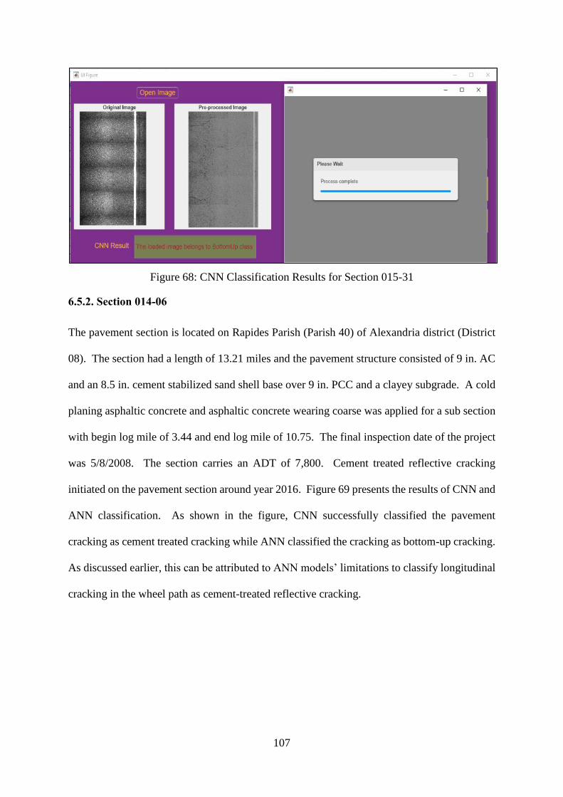
107
Figure 68: CNN Classification Results for Section 015-31
6.5.2. Section 014-06
The pavement section is located on Rapides Parish (Parish 40) of Alexandria district (District
08). The section had a length of 13.21 miles and the pavement structure consisted of 9 in. AC
and an 8.5 in. cement stabilized sand shell base over 9 in. PCC and a clayey subgrade. A cold
planing asphaltic concrete and asphaltic concrete wearing coarse was applied for a sub section
with begin log mile of 3.44 and end log mile of 10.75. The final inspection date of the project
was 5/8/2008. The section carries an ADT of 7,800. Cement treated reflective cracking
initiated on the pavement section around year 2016. Figure 69 presents the results of CNN and
ANN classification. As shown in the figure, CNN successfully classified the pavement
cracking as cement treated cracking while ANN classified the cracking as bottom-up cracking.
As discussed earlier, this can be attributed to ANN models’ limitations to classify longitudinal
cracking in the wheel path as cement-treated reflective cracking.

108
Figure 69: CNN and ANN Classification Results for Section 014-06
6.5.3. Section 027-04
The pavement section is located on Webster parish (Parish 60) of Bossier City district (District
04). The section had a length of 8.19 miles and the pavement structure consisted of 7.25 in.
AC and a 4.5 in. cement stabilized sand shell base over a stone subbase and clay subgrade. An
asphaltic concrete pavement resurfacing was applied for a sub section with begin log mile of
2.37 and end log mile of 8.18. The final inspection date of the project was 5/17/2006. The
section carries an ADT of 11,800. The section developed typical cement-treated reflective
cracks at year 2016 and the cracks initiated as transverse cracks at the year 2012. Figure 70
presents the results of CNN and ANN classification. As shown in the figure, both CNN and
ANN successfully classified surface cracking as cement-treated reflective cracking.
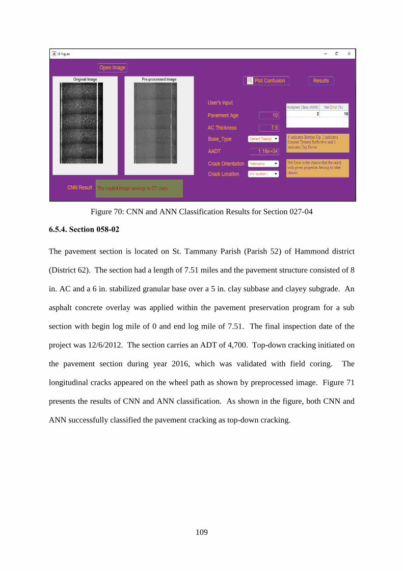
109
Figure 70: CNN and ANN Classification Results for Section 027-04
6.5.4. Section 058-02
The pavement section is located on St. Tammany Parish (Parish 52) of Hammond district
(District 62). The section had a length of 7.51 miles and the pavement structure consisted of 8
in. AC and a 6 in. stabilized granular base over a 5 in. clay subbase and clayey subgrade. An
asphalt concrete overlay was applied within the pavement preservation program for a sub
section with begin log mile of 0 and end log mile of 7.51. The final inspection date of the
project was 12/6/2012. The section carries an ADT of 4,700. Top-down cracking initiated on
the pavement section during year 2016, which was validated with field coring. The
longitudinal cracks appeared on the wheel path as shown by preprocessed image. Figure 71
presents the results of CNN and ANN classification. As shown in the figure, both CNN and
ANN successfully classified the pavement cracking as top-down cracking.

110
Figure 71: CNN and ANN Classification Results for Section 058-02
6.5.5. Section 262-03
The pavement section is located on Livingston Parish (Parish 32) of Hammond district (District
62). The section had a length of 6.41 miles and the pavement structure consisted of 8.5 in. AC
and a 5.5 in. base over a clay subgrade. A cold planing, patching, and asphalt concrete overlay
treatment was applied for a sub section with begin log mile of 0 and end log mile of 6.41. The
final inspection date of the project was 12/17/2013. The section carries an ADT of 15,000.
Top-down cracking initiated on the pavement section during year 2016, which was validated
with field coring. Figure 72 presents the results of CNN and ANN classification.
Figure 72: CNN and ANN Classification Results for Section 262-03

111
The longitudinal cracks appeared on the wheel path as shown in the processed image.
As shown in the figure, both CNN and ANN successfully classified the pavement cracking as
top-down cracking.
6.5.6. Section 266-01
The pavement section is located on Ascension Parish (Parish 03) of Baton Rouge district
(District 61). The section had a length of 9.75 miles and the pavement structure consisted of
14 in. AC and over a clay subgrade. A patch and overlay treatment was applied for a sub
section with begin log mile of 0 and end log mile of 4.44. The final inspection date of the
project was 4/26/2013. The section carries an ADT of 5,600. Top-down cracking initiated on
the pavement section during year 2015, which was validated with field coring. The
longitudinal cracks appeared on the wheel path as shown in the processed image. Figure 73
presents the results of CNN and ANN classification. As shown in the figure, both CNN and
ANN successfully classified the pavement cracking as top-down cracking.
Figure 73: CNN and ANN Classification Results for Section 266-01

112
6.5.7. Section 829-26
The pavement section is located on Lafourche Parish (Parish 29) of Bridge City district
(District 02). The section had a length of 16.07 miles and the pavement structure consisted of
9 in. AC and 12 in. granular base over a 14 in. sand subbase and sand subgrade. A cold planing
and overlay of the existing asphaltic concrete was applied for a sub section with begin log mile
of 11.78 and end log mile of 16.07. The final inspection date of the project was 7/12/2013.
The section carries an ADT of 13,500. Top-down cracking initiated on the pavement section
during year 2015, which was validated with field coring. The longitudinal cracks appeared on
the wheel path as shown in the processed image. Figure 74 presents the results of CNN and
ANN classification. As shown in the figure, both CNN and ANN successfully classified the
pavement cracking as top-down cracking.
Figure 74: CNN and ANN Classification Results for Section 829-26
6.5.8. Section 857-63
The pavement section is located on Vermilion Parish (Parish 57) of Lafayette district (District
03). The section had a length of 10.79 miles and the pavement structure consisted of 3.5 in.
AC and 9.5 in. cement stabilized sand clay gravel base over a clay subgrade. A base
stabilization and asphalt overlay was applied for a sub section with begin log mile of 0.65 and
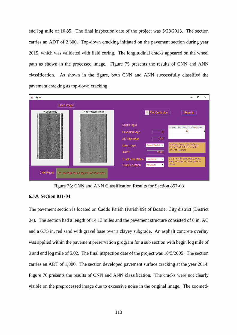
113
end log mile of 10.85. The final inspection date of the project was 5/28/2013. The section
carries an ADT of 2,300. Top-down cracking initiated on the pavement section during year
2015, which was validated with field coring. The longitudinal cracks appeared on the wheel
path as shown in the processed image. Figure 75 presents the results of CNN and ANN
classification. As shown in the figure, both CNN and ANN successfully classified the
pavement cracking as top-down cracking.
Figure 75: CNN and ANN Classification Results for Section 857-63
6.5.9. Section 011-04
The pavement section is located on Caddo Parish (Parish 09) of Bossier City district (District
04). The section had a length of 14.13 miles and the pavement structure consisted of 8 in. AC
and a 6.75 in. red sand with gravel base over a clayey subgrade. An asphalt concrete overlay
was applied within the pavement preservation program for a sub section with begin log mile of
0 and end log mile of 5.02. The final inspection date of the project was 10/5/2005. The section
carries an ADT of 1,000. The section developed pavement surface cracking at the year 2014.
Figure 76 presents the results of CNN and ANN classification. The cracks were not clearly
visible on the preprocessed image due to excessive noise in the original image. The zoomed-

114
in preprocessed picture showed longitudinal cracks on the wheel path. As shown in the figure,
both CNN and ANN classified the pavement cracking as bottom-up cracking.
Figure 76: CNN and ANN Classification Results for Section 011-04
6.5.10. Section 003-10
The pavement section is located on Acadia parish (Parish 01) of Lafayette district (District 03).
The section had a length of 11.367 miles and the pavement structure consisted of 6 in. AC and
a 7.5 in. Portland Cement Concrete (PCC) base over a clay subgrade. An asphaltic concrete
overlay was applied for a sub section with begin log mile of 6.28 and end log mile of 11.377.
The final inspection date of the project was 8/13/2012. The section carries an ADT of 6,700.
The section developed pavement surface cracks at year 2016. Figure 77 presents the results of
CNN and ANN classification. As shown in the figure, both CNN and ANN classified surface
cracking as cement-treated reflective cracking.

115
Figure 77: CNN and ANN Classification Results for Section 003-10
6.5.11. Section 015-05
The pavement section is located on La Salle Parish (Parish 30) of Chase district (District 58).
The section had a length of 13.420 miles and the pavement structure consisted of 9 in. AC and
7 in. RAP/grave mixture base over a sand subgrade. A cold planing and overlay of the existing
asphaltic concrete was applied for a sub section with begin log mile of 3.726 and end log mile
of 9.711. The final inspection date of the project was 10/15/2012. The section carries an ADT
of 6,300. Pavement surface cracking initiated on the pavement section during year 2016. The
longitudinal cracks appeared on the wheel path as shown in the processed image. Figure 78
presents the results of CNN and ANN classification. As shown in the figure, both CNN and
ANN classified the pavement cracking as top-down cracking.

116
Figure 78: CNN and ANN Classification Results for Section 015-05
6.5.12. Section 010-06
The pavement section is located on Bossier parish (Parish 08) of Bossier City district (District
04). The section had a length of 15.221 miles and the pavement structure consisted of 3.5 in.
AC and 8.75 in. PCC base over a sand subgrade. A milling and overlay was applied for a sub
section with begin log mile of 8.106 and end log mile of 13.148. The final inspection date of
the project was 5/1/2013. The section carries an ADT of 16,800. Pavement surface cracking
initiated on the pavement section during year 2016. The longitudinal cracks appeared on the
wheel path as shown in the processed image. The section also developed transverse cracking
during the year 2016. Figure 79 presents the results of CNN and ANN classification. As shown
in the figure, CNN and ANN classified the pavement cracking as top-down cracking and
cement-treated reflective cracking.

117
Figure 79: CNN and ANN Classification Results for Section 010-06
6.5.13. Section 424-08
The pavement section is located on Lafourche parish (Parish 29) of Bridge City district (District
02). The section had a length of 15.252 miles and the pavement structure consisted of 10 in.
AC and a 7.5 in. cement stabilized sand shell base over a clay subgrade. An asphaltic concrete
overlay was applied for a sub section with begin log mile of 0 and end log mile of 7. The final
inspection date of the project was 3/19/2014. The section carries an ADT of 21,500. The
section developed pavement surface cracks at year 2018. Figure 80 presents the results of CNN

118
and ANN classification. As shown in the figure, both CNN and ANN classified surface
cracking as cement-treated reflective cracking.
Figure 80: CNN and ANN Classification Results for Section 424-08
6.5.14. Section 426-01
The pavement section is located on Ascension parish (Parish 03) of Baton Rouge district
(District 61). The section had a length of 4.483 miles and the pavement structure consisted of
11 in. AC and a 8 in. cement stabilized sand shell base over a sand subgrade. A cold planing
and asphaltic concrete overlay was applied for a sub section with begin log mile of 0 and end
log mile of 2.78. The final inspection date of the project was 12/4/2013. The section carries
an ADT of 16,200. The section developed pavement surface cracks at year 2017. Figure 81
presents the results of CNN and ANN classification. As shown in the figure, CNN and ANN
classified surface cracking as cement-treated reflective cracking.

119
Figure 81: CNN and ANN Classification Results for Section 426-01

120
CONCLUSIONS AND RECOMMENDATIONS
The objective of this dissertation was twofold, which was achieved in two phases. In the first
phase, this study developed the CNN tool to classify pavement cracking as top-down, bottom-
up, and cement treated reflective cracking from digital pavement image and ANN tool as
decision making tool to validate the classification of CNN tool. In the second phase, finite
element models were constructed to identify the specific cause and locations of these cracks.
Based on the results of the study, the following are concluded:
CNN and ANN Models
The primary objective of the study was to identify and classify top-down, bottom-up, and
cement treated reflective cracking in in-service flexible pavements without core extraction or
other destructive tools. To achieve this objective, an image-based CNN model was developed
that analyze the characteristics of pavement surface images. Furthermore, a one-step decision-
making tool was developed using ANN to cross validate the crack classification obtained from
the imaged-based CNN. To achieve this objective, 350 pavement images were pre-processed
and were used as inputs for training, testing, and validation of the CNN model.
The input database for the CNN model contained both high quality pavement images
with distinct cracks and images with high complexity such as cracks on shadowed surface,
highly textured pavement surface, blurry cracks, and surfaces with poor background
illumination and high intensity variation. For unprocessed pavement images, the model
achieved an accuracy of 61.7% and 73.4% on testing and validation phases, respectively. The
lower accuracy can be attributed to the presence of excessive pavement noise, non-uniform
background illumination, pavement marking, spots and stains including cracking pattern. For
the data set consisting of 2D images only, the developed network achieved an overall accuracy
of 88.9% and 86.7% in the testing and validation phases, respectively. The overall accuracy

121
for 2D and 3D images was 93.8% and 91% in the testing and validation phases, respectively.
An ANN-based pattern recognition system was trained and validated based on pavement age,
AC thickness, AADT, base type, crack orientation, and crack location to further validate the
image-based classification. The developed model showed an acceptable decision prediction
accuracy of 92%. Based on the overall accuracy, the approach of using pre-trained
convolutional neural network model was observed to be successful for automated pavement
crack classification.
Finite Element Modelling
Flexible pavement responses under a dual tire assembly and due to shrinkage in cement-treated
layers was studied to identify the critical stress mechanisms for fatigue cracking, top-down
cracking, and cement-treated reflective cracking. Three dimensional (3D) finite element
models (FE) were developed to simulate typical pavement structures used for low, medium,
and high traffic volumes. The loading pattern for dual-tire configurations was simulated in the
developed 3D FE models to calculate the tensile strains at various locations on the pavement.
Furthermore, shrinkage cracking in cement treated base (CTB) was modeled in finite element
using displacement boundary conditions. Based on the results of the FE analysis, the following
conclusions may be drawn:
Higher tensile strains were observed to occur underneath the tire ribs than away from
them supporting the field observations that both surface initiated and bottom-up fatigue
cracking develop in or near the wheel paths.
The incorporation of surface transverse tangential stresses increased the surface tensile
strains near the tire ribs by approximately 68%, 63%, and 53% respectively for
pavements used for low, medium, and high traffic volumes indicating an increased
potential for the initiation and development of top-down cracking.

122
The effect of surface tangential stresses was observed to be minimal for tensile strains
at bottom of the AC layer. The tensile strains only increased by 7%, 6%, and 3% for
pavements used for low, medium, and high volumes.
The longitudinal tangential stresses were observed to have negligible effect on the
tensile strains both at the top and bottom of the AC layer. The increase in tensile strains
at the pavement surface and at the bottom of the AC layer was less than 5% and less
than 1%, respectively, for all types of flexible pavements.
Results also indicated that thin pavements used for low traffic volume had a higher
probability of developing bottom-up fatigue cracking.
The tensile strain at the pavement surface was observed to decrease with the increase
in AC layer thickness. In addition, the increase in tensile strain at the pavement surface
with the incorporation of tangential stresses was approximately 60% for all pavements.
The tensile strain at bottom of AC layer increased by approximately 9% for pavement
with 38.1mm (1.5 in.) AC layer with the incorporation of tangential loading while the
increase was only 1.5% for pavement with 203.2mm (8 in.) thick AC.
The increased stiffness of the AC surface mixes offer more resistance to the vertical
and tangential loading at the pavement surface, thus reducing top-down cracking
potential.
The tensile stresses due to shrinkage strains in cement treated base were observed to be
higher than the tensile strength of the material at 56 days indicating the potential
development of shrinkage cracks within few weeks after construction. These cracks
propagate through the AC layer over time and appear as cement treated reflective cracks
at the surface.

123
The addition of fly ash reduced the tensile stresses in cement treated base by
approximately 49% at 46 days resulting in a significant reduction in the cracking
potential of the CTB after construction.
Recommendations
The present study developed an image-based CNN model to classify pavement cracks as top-
down, bottom-up, and cement-treated reflective cracking. While this study is the attempt to
classify pavement cracks with respect to their initiation and propagation, the results of this
study indicate the need for further improvements with more data set and use of much advanced
computer programming. The major limitations and recommendations of the study are listed
hereunder:
The training, testing, and validation data set for the developed CNN model consisted of
pavement images with known crack types. Further testing on the accuracy of the
developed model is recommended by using pavement images with different crack types
and core extraction.
The pavement network in Louisiana is surveyed every two years. However, due to the
inconsistencies in the pavement images before and after the year 2012, only the images
after 2012 were used. This limited the number of images for each crack type in the
developed model. Further improvement of the model is recommended as more data
become available.
The automated image processing step involved crack enhancement by using few
mathematical operations. It is recommended to expand the developed methodology in
order to increase crack classification accuracy in flexible pavements. This can be
achieved by using advanced image processing techniques or a deep learning CNN that
can automatically perform crack segmentation.

124
Overall, the developed novel methodology is a promising approach to assist DOTs in crack
classification of top-down, bottom-up, and cement treated reflective cracks, based on the
surface characteristics of these cracks and pavement attributes.

125
APPENDIX. CNN CODE FOR IMAGE CLASSIFICATION
outputFolder = fullfile('CNN Inputs');
rootFolder = fullfile(outputFolder,'Cracks');
categories = {'BottomUp', 'CT', 'TopDown'};
imds = imageDatastore(fullfile(rootFolder,categories),'LabelSource','Foldernames');
tbl = countEachLabel(imds);
minSetCount = min(tbl{:,2});
imds = splitEachLabel(imds, 0.9, 'randomize');
countEachLabel(imds);
BottomUp = find(imds.Labels == 'BottomUp',1);
CT = find(imds.Labels == 'CT',1);
TopDown = find(imds.Labels == 'TopDown',1);
net = alexnet ();
rng('default');
net.Layers(1);
net.Layers(end);
numel(net.Layers(end).ClassNames);
[trainingSet, testSet, validationSet] = splitEachLabel(imds, 0.6, 0.15, 'randomize');
imageSize = net.Layers(1).InputSize;
augmentedTrainingSet =
augmentedImageDatastore(imageSize,trainingSet,'ColorPreprocessing','gray2rgb');
augmentedTestSet =
augmentedImageDatastore(imageSize,testSet,'ColorPreprocessing','gray2rgb');
augmentedValidationSet =
augmentedImageDatastore(imageSize,validationSet,'ColorPreprocessing','gray2rgb');
w1 = net.Layers(2).Weights;
w1 = mat2gray(w1);
featurelayer = 'drop7';
trainingFeatures = activations(net, augmentedTrainingSet, featurelayer,'MiniBatchSize',
32,'OutputAs', 'columns');
miniBatchSize = 25;
options = trainingOptions('sgdm', ...
'LearnRateSchedule','piecewise',...
'LearnRateDropFactor',0.5, ...
'LearnRateDropPeriod',5, ...
'MaxEpochs',8, ...
'MiniBatchSize',25, ...
'Plots','training-progress',...
'Shuffle','once');
numClasses = 3;

126
layersTransfer = net.Layers(1:end-3);
layers = [
layersTransfer
fullyConnectedLayer(numClasses,'WeightLearnRateFactor',20,'BiasLearnRateFactor',20)
softmaxLayer
classificationLayer];
trainedNet = trainNetwork(augmentedTrainingSet,layers,options);
trainingLabels = trainingSet.Labels;
classifier = fitcecoc(trainingFeatures, trainingLabels, 'Learner', 'Linear', 'Coding',
'onevsall','observationsIn','columns');
testFeatures = activations(trainedNet,augmentedTestSet, featurelayer,'MiniBatchSize',
32,'OutputAs', 'columns');
validationFeatures = activations(trainedNet,augmentedValidationSet,
featurelayer,'MiniBatchSize', 32,'OutputAs', 'columns');
predictLabels = predict(classifier,testFeatures,'ObservationsIn','columns');
predictLabelss = predict(classifier,validationFeatures,'ObservationsIn','columns');
testLables = testSet.Labels;
validationLables = validationSet.Labels;
confMat = confusionmat(testLables, predictLabels);
confMatt = confusionmat(validationLables, predictLabelss);
confMat = bsxfun(@rdivide, confMat, sum(confMat,2));
confMatt = bsxfun(@rdivide, confMatt, sum(confMatt,2));
mean(diag(confMat));
mean(diag(confMatt));
newImage = imread(fullfile('*.tif'));
ds = augmentedImageDatastore(imageSize,newImage,'ColorPreprocessing','gray2rgb');
imageFeatures = activations(trainedNet, ds, featurelayer, 'MiniBatchSize', 32,'OutputAs',
'columns');
label = predict(classifier,imageFeatures, 'ObservationsIn','columns');
sprintf('The loaded image belongs to %s class', label)
plotconfusion(testLables, predictLabels)
plotconfusion(validationLables, predictLabelss)

127
REFERENCES
Abdel-Qader, I., Abudayyeh, O., and Kelly, M. E. Analysis of edge-detection techniques for
crack identification in bridges. Journal of Computing in Civil Engineering, 17(4), 255-
263, 2003.
Akbulut, H., and Aslantas, K. Finite element analysis of stress distribution on bituminous
pavement and failure mechanism. Materials & design, 26(4), 383-387, 2005.
Al-Qadi, I. L., Elseifi, M., & Leonard, D. Development of an overlay design model for
reflective cracking with and without steel reinforcing nettings. Asphalt Paving
Technology, 72, 388-423, 2003.
Al-Qadi, I. L., Loulizi, A., Elseifi, M., and Lahouar, S. The Virginia Smart Road: The impact
of pavement instrumentation on understanding pavement performance. Journal of the
Association of Asphalt Paving Technologists, 73(3), 427-465, 2004.
Al-Qadi, I. L., Elseifi, M. A., and Yoo, P. J. Characterization of pavement damage due to
different tire configurations. Journal of the Association of Asphalt Paving Technologists,
74, 921-962, 2005.
Al-Qadi, I. L., Elseifi, M. A., Yoo, P. J., and Janajreh, L. Mechanistic quantification of
pavement damage due to dual and wide-base tires. Tire Sciences and Technology, 33(4),
pp. 210-226, 2005.
Al-Qadi, I. L., and Yoo, P. J. Effect of surface tangential contact stresses on flexible
pavement response. Journal of the Association of Asphalt Paving Technologists, 76(8),
663-692, 2007.
Al-Qadi, I., Wang, H., Yoo, P. and Dessouky, S. Dynamic analysis and in situ validation of
perpetual pavement response to vehicular loading. Transportation Research Record:
Journal of the Transportation Research Board, (2087), pp.29-39, 2008.
Ameri, M., Mansourian, A., Khavas, M. H., Aliha, M. R. M., and Ayatollahi, M. R. Cracked
asphalt pavement under traffic loading–A 3D finite element analysis. Engineering
Fracture Mechanics, 78(8), 1817-1826, 2011.
Ayenu-Prah, A., and Attoh-Okine, N. Evaluating pavement cracks with bidimensional
empirical mode decomposition. EURASIP Journal on Advances in Signal Processing,
2008(1), 861701, 2008.
Birgisson, B., Sangpetngam, B., and Roque, R. Predicting viscoelastic response and crack
growth in asphalt mixtures with the boundary element method. Transportation Research
Record, 1789(1), 129-135, 2002.
Cho, Y. H., Lee, K. W., and Ryu, S. W. Development of cement-treated base material for
reducing shrinkage cracks. Transportation research record, 1952(1), 134-143, 2006.
Cho, Y. H., McCullough, B., and Weissmann, J. Considerations on finite-element method
application in pavement structural analysis. Transportation Research Record: Journal of
the Transportation Research Board, Vol. 1539, pp. 96-101, 1996.

128
Dave, E. V., Song, S. H., Buttlar, W. G., and Paulino, G. H. Reflective and thermal cracking
modeling of asphalt concrete overlays. Advanced Testing and Characterization of
Bituminous Materials, 2, 1241-1252, 2007.
De Freitas, E. F., Pereira, P., Picado–Santos, L., and Papagiannakis, A. T. Effect of
construction quality, temperature, and rutting on initiation of top-down cracking.
Transportation research record, 1929(1), 174-182, 2005.
Deng, X., Q. Liu, Y. Deng, and Mahadevan, S. An improved method to construct basic
probability assignment based on the confusion matrix for classification problem.
Information Sciences, Vol. 340-341,pp. 250–261, 2016.
Eisenbach, M., Stricker, R., Seichter, D., Amende, K., Debes, K., Sesselmann, M., and Gross,
H. M. How to get pavement distress detection ready for deep learning? A systematic
approach. In 2017 international joint conference on neural networks (IJCNN) (pp. 2039-
2047). IEEE, 2017.
Elseifi, M. Performance quantification of interlayer systems in flexible pavements using
finite element analysis, instrument response, and non destructive testing (Doctoral
dissertation, Virginia Tech), 2003.
Elseifi, M. Analysis of seasonal strain measurements in asphalt materials under accelerated
pavement testing and comparing field performance and laboratory measured binder
tension properties. Report No. FHWA/LA. 09/444, Louisiana Transportation Research
Center, 2009.
Elseifi, M. A., and Elbagalati, O. Assessment of continuous deflection measurement devices
in Louisiana-rolling wheel deflectometer. Final report 581 (No. FHWA/LA. 17/581).
Louisiana Transportation Research Center, 2017.
Elseifi, M. A., Mohammad, L. N., Ying, H., and Cooper III, S. Modeling and evaluation of
the cracking resistance of asphalt mixtures using the semi-circular bending test at
intermediate temperatures. Road Materials and Pavement Design, 13(sup1), pp. 124-139,
2012.
Elseifi, M. A., and Zihan, Z. U. Assessment of the traffic speed deflectometer in Louisiana
for pavement structural evaluation (No. FHWA/LA. 18/590). Louisiana Transportation
Research Center, 2018.
Fan, Z., Wu, Y., Lu, J., and Li, W. Automatic pavement crack detection based on structured
prediction with the convolutional neural network. arXiv preprint arXiv:1802.02208, 2018.
Georgopoulos, A., Loizos, A., and Flouda, A. Digital image processing as a tool for
pavement distress evaluation. ISPRS Journal of Photogrammetry and Remote Sensing,
50(1), pp. 23-33, 1995.
Gopalakrishnan, K. Deep Learning in data-driven pavement image analysis and automated
distress detection: A review. Data 3, no. 3: 28, 2018.
Gopalakrishnan, K., Khaitan, S. K., Choudhary, A., and Agrawal, A. Deep convolutional
neural networks with transfer learning for computer vision-based data-driven pavement
distress detection. Construction and Building Materials, 157, 322-330, 2017.

129
Gribniak, V., Kaklauskas, G., and Bacinskas, D. Shrinkage in reinforced concrete structures:
a computational aspect. Journal of civil engineering and management, 14(1), 49-60, 2008.
Hadi, M. N. and Bodhinayake, B. C. Non-linear finite element analysis of flexible pavements.
Advances in Engineering Software, 34(11-12), pp.657-662, 2003.
Nhat-Duc, H., Nguyen, Q. L., and Tran, V. D. Automatic recognition of asphalt pavement
cracks using metaheuristic optimized edge detection algorithms and convolution neural
network. Automation in Construction, 94, 203-213, 2018.
Hu, Y., and Zhao, C. X. A novel LBP based methods for pavement crack detection. Journal
of pattern Recognition research, 5(1), 140-147, 2010.
Huang, Y. H. Pavement analysis and design. 1st ed., Prentice Hall, NJ, 1993.
Jahanshahi, M. R., Kelly, J. S., Masri, S. F., and Sukhatme, G. S. A survey and evaluation of
promising approaches for automatic image-based defect detection of bridge structures.
Structure and Infrastructure Engineering, 5(6), 455-486, 2009.
Karlaftis, M., and Vlahogianni, E. Statistical methods versus neural networks in
transportation research: Differences, Similarities and Some Insights. Transportation
Research Part C: Emerging Technologies, Vol. 19, No. 3, pp. 387–399, 2011.
Khattak, M. J., Baladi, G. Y., Zhang, Z., and Ismail, S. A review of the pavement
management system of the state of Louisiana-phase. Transportation Research Record:
Journal of the Transportation Research Board, pp. 18-27, 2008.
Kim, J., Roque, R., and Byron, T. Viscoelastic analysis of flexible pavements and its effects
on top-down cracking. Journal of Materials in Civil Engineering, 21(7), 324-332, 2009.
Kim, M., Burton, Y. M., Prozzi, J. A., and Murphy, M. Maintenance and rehabilitation
project selection using artificial neural networks. Transportation Research Board 93rd
Annual Meeting, No. 14-3620, 2014.
Kim, M., Mohammad, L. N., and Elseifi, M. A. Characterization of fracture properties of
asphalt mixtures as measured by semicircular bend test and indirect tension test.
Transportation research record, 2296(1), 115-124, 2012.
King, W. M., and Abadie. C. Comparative performance of conventional and rubberized hot
mix under accelerated loading – construction report. FHWA/LA-99/331, Louisiana
Transportation Research Center, Louisiana Department of Transportation, Baton Rouge,
LA, 1999.
Kittler, J., and Illingworth, J. Minimum error thresholding. Pattern recognition, 19(1), 41-47,
1986.
Koch, C., Georgieva, K., Kasireddy, V., Akinci, B., and Fieguth, P. A review on computer
vision based defect detection and condition assessment of concrete and asphalt civil
infrastructure. Advanced Engineering Informatics, 29(2), 196-210, 2015.
Koutsopoulos, H. N., and Downey, A. B. Primitive-based classification of pavement cracking
images. Journal of Transportation Engineering, 119, no. 3, pp. 402-418, 1993.

130
Krizhevsky, A., Sutskever, I., and Hinton, G. E. Imagenet classification with deep
convolutional neural networks. In Advances in neural information processing systems,
pp. 1097-1105, 2012.
“LADOTD Pavement Management System Guide” 2006.
Leverington, D. (2012). A basic introduction to feedforward backpropagation neural
networks. Neural Network Basics.
Li, B., Wang, K. C., Zhang, A., Yang, E., and Wang, G. Automatic classification of
pavement crack using deep convolutional neural network. International Journal of
Pavement Engineering, 1-7, 2018.
Li, L., Chan, P., Rao, A., and Lytton, R. L. Flexible pavement distress evaluation using image
analysis. In Applications of Advanced Technologies in Transportation Engineering,
ASCE, pp. 473-477, 1991.
Li, S., and Zhao, X. Image-based concrete crack detection using convolutional neural
network and exhaustive search technique. Advances in Civil Engineering, 2019.
Lim, S., Kestner, D., Zollinger, D. G., and Fowler, D. W. Characterization of crushed
concrete materials for paving and non-paving applications. Research Report 4954-1,
2003.
Lytton, R. L., Uzan, J., Fernando, E. G., Roque, R., Hiltunen, D., and Stoffels, S. M.
Development and validation of performance prediction models and specifications for
asphalt binders and paving mixes. Washington, DC: Strategic Highway Research
Program, Vol. 357, 1993.
Maeda, H., Sekimoto, Y., Seto, T., Kashiyama, T., and Omata, H. Road damage detection
using deep neural networks with images captured through a smartphone. arXiv preprint
arXiv:1801.09454, 2018.
Maode, Y., Shaobo, B., Kun, X., and Yuyao, H. Pavement crack detection and analysis for
high-grade highway. In 2007 8th International Conference on Electronic Measurement
and Instruments (pp. 4-548). IEEE, 2007.
Maser, K. R. Computational techniques for automating visual inspection. Massachusetts
Institute of Technology, Report, Cambridge, MA, 1987.
Mohammad, L. N., Raghavandra, A., and Huang, B. Laboratory performance evaluation of
cement-stabilized soil base mixtures. Transportation research record, 1721(1), 19-28,
2000.
Mohammad, L. N., Masood Rasoulian, P. E., Bill King, P. E., Martinez, M., and Qi, Y.
Evaluation of stone/RAP interlayers under accelerated loading. Report No. FHWA
LA.06/409, Louisiana Transportation Research Center, 2008.
Mokhtari, S., Wu, L., and Yun, H. B. Comparison of supervised classification techniques for
vision-based pavement crack detection. Transportation Research Record, 2595(1), 119-
127, 2016.

131
Moussa, G., and Hussain, K. A new technique for automatic detection and parameters
estimation of pavement crack. In 4th International Multi-Conference on Engineering
Technology Innovation, IMETI, 2011.
Myers, L. A., Roque, R., and Ruth, B. E. Mechanisms of surface-initiated longitudinal wheel
path cracks in high-type bituminous pavements. Journal of the Association of Asphalt
Paving Technologists, 67, 1998.
Nguyen, T. S., Avila, M., and Begot, S. Automatic detection and classification of defect on
road pavement using anisotropy measure. In 2009 17th European Signal Processing
Conference (pp. 617-621). IEEE, 2009.
Otsu, N. A threshold selection method from gray-level histograms. IEEE transactions on
systems, man, and cybernetics, 9(1), 62-66, 1979.
Plati, C., Georgiou, P. and Papavasiliou, V. Simulating pavement structural condition using
artificial neural networks. Structure and Infrastructure Engineering, pp. 1–10, 2015.
Preciado, J., Arguelles, G. M., Dugarte, M., Bonicelli, A., Cantero, J., Vega, D., and Barros,
Y. Improving mechanical properties of hot mix asphalt using fibres and polymers in
developing countries. In IOP Conference Series: Materials Science and Engineering (Vol.
245, No. 2, p. 022013). IOP Publishing, 2017.
Romanoschi, S. A., and Metcalf, J. B. Characterization of asphalt concrete layer interfaces.
Transportation Research Record, 1778(1), 132-139, 2001.
Roque, R., Birgisson, B., Drakos, C., and Dietrich, B. Development and field evaluation of
energy-based criteria for top-down cracking performance of hot mix asphalt (with
discussion). Journal of the Association of Asphalt Paving Technologists, 73, 2004.
Simulia, D. ABAQUS 6.11 Theory Manual. Providence, RI, USA: DS SIMULIA Corp,
2011.
Simulia, D. S. ABAQUS 6.13 User’s Manual. Dassault Systems, Providence, RI, 2013.
Some, L. Automatic image-based road crack detection methods. 2016.
Song, K. Y., Petrou, M., and Kittler, J. Texture crack detection. Machine Vision and
Applications, 8(1), 63-75, 1995.
Stuart, K., Mogawer, W., Romero, P. Validation of the superpave asphalt binder fatigue
cracking parameter using an accelerated loading facility. Publication No. FHWA- RD-01-
093. Turner Fairbank Highway Research Centre, McLean, VA, 2001.
Subirats, P., Dumoulin, J., Legeay, V., and Barba, D. Automation of pavement surface crack
detection using the continuous wavelet transform. In 2006 International Conference on
Image Processing (pp. 3037-3040). IEEE, 2006.
Svasdisant, T., Schorch, M., and Baladi, G. Y. Mechanistic analysis of top-down cracks in
asphalt pavements. Paper presented in Transportation Research Board Annual Meeting,
January 13-17, 2002.

132
Taherkhani, H., and Arshadi, M. R. Investigating the mechanical properties of asphalt
concrete containing waste polyethylene terephthalate. Road Materials and Pavement
Design, 20(2), 381-398, 2019.
Tielking, J. T., and Roberts, F. L. Tire contact pressure and its effect on pavement strain.
Journal of Transportation Engineering, 113(1), 56-71, 1987.
Tong, Z., Gao, J., and Zhang, H. Recognition, location, measurement, and 3D reconstruction
of concealed cracks using convolutional neural networks. Construction and Building
Materials, 146, 775-787, 2017.
Uhlmeyer, J. S., Willoughby, K., Pierce, L. M., and Mahoney, J. P. Top-down cracking in
Washington state asphalt concrete wearing courses. Transportation research record,
1730(1), 110-116, 2000.
Wang, H. and Al-Qadi, I. Combined effect of moving wheel loading and three-dimensional
contact stresses on perpetual pavement responses. Transportation Research Record:
Journal of the Transportation Research Board, (2095), pp.53-61, 2009.
Wang, X., and Hu, Z. Grid-based pavement crack analysis using deep learning. In 2017 4th
International Conference on Transportation Information and Safety (ICTIS), pp. 917-924.
IEEE, 2017.
Wu, L., Mokhtari, S., Nazef, A., Nam, B., and Yun, H.B. Improvement of crack-detection
accuracy using a novel crack defragmentation technique in image-based road assessment.
Journal of Computing in Civil Engineering, 30(1), 04014118, 2014.
Wu, Z., Zhang, Z., and King Jr, W. M. Accelerated loading evaluation of stabilized BCS
layers in pavement performance. Report No. FHWA/LA. 08/474, 2012.
Xiao, Y. Evaluation of engineering properties of hot mix asphalt concrete for the
mechanistic-empirical pavement design. 2009.
Xu, B., Huang, Y. R. Development of an automatic pavement surface distress inspection
system. Report No. FHWA/TX-05/7-4975-1, 2003.
Ying, L., and Salari, E. Beamlet transform based technique for pavement image processing
and classification. In Electro/Information Technology, 2009. eit'09. IEEE International
Conference on, pp. 141-145, IEEE, 2009.
Yoo, P. J., Al-Qadi, I. L., Elseifi, M. A., and Janajreh, I. Flexible pavement responses to
different loading amplitudes considering layer interface condition and lateral shear forces.
The International Journal of Pavement Engineering, 7(1), 73-86, 2006.
Zaghloul, S. M. and White, T. Use of a three-dimensional, dynamic finite element program
for analysis of flexible pavement. Transportation research record, (1388), 1993.
Zhang, L., Yang, F., Zhang, Y. D., and Zhu, Y. J. Road crack detection using deep
convolutional neural network. In 2016 IEEE international conference on image
processing (ICIP) (pp. 3708-3712). IEEE, 2016.

133
Zhou, J., Huang, P. S., and Chiang, F. P. Wavelet-based pavement distress detection and
evaluation. Optical Engineering, 45(2), 027007, 2006.
Zou, Q., Cao, Y., Li, Q., Mao, Q., and Wang, S. CrackTree: Automatic crack detection from
pavement images. Pattern Recognition Letters, 33(3), 227-238, 2012

134
VITA
Nirmal Dhakal was born in April 1988, in Lekhnath-09, Kaski, Nepal. He began his studies
from Global Collegiate Higher Secondary School, Pokhara, and later completed his high school
from SOS Hermann Gmeiner School, Gandaki. He completed his undergraduate study from
Institute of Engineering, Pulchowk Campus, obtaining his Bachelor degree in Civil
Engineering in December 2011. He received his Master’s degree in Civil Engineering from
Louisiana State University in August 2016. He was admitted to the graduate school of
Louisiana State University for the Ph.D. program in January 2018, where he worked as a
research assistant under Dr. Mostafa Elseifi and completed his research successfully in March
2020. He is expected to receive Doctor of Philosophy degree in Civil Engineering in summer
of 2020.


