Hydrologic and Paleohydrologic Assessment of the 1993 Floods on the Verde River,
Central Arizona
by
P. Kyle House, Philip A. Pearthree, and Jonathan E. Fuller'
Arizona Geological Survey Open-File Report 95-20
December 1995
Arizona Geological Survey 416 W. Congress, Suite #100, Tucson, Arizona 85701
JE Fuller/Hydrology and Geomorphology, Inc.
Contribution #46 from the Arizona Laboratory for Paleohydrological and Hydroclimatological Analysis (ALPHA)
Researchfunded by the Salt River Project, the Hydrological Sciences Program o/the National Science Foundation, and the Arizona Geological Survey
This report is preliminary and has not been edited or reviewed for conformity with Arizona Geological Survey standards


Abstract
The Verde River experienced very large floods in January and February of 1993 during a major episode of flooding that affected most of the large drainages in Arizona. The January flood peak discharge on the lower Verde River (4,100 m3
S-l) was the largest of the gage record, and the February flood peak (3,650 m3
S-l) was the second largest. These large, very recent floods provide an exceptional opportunity to investigate the genesis oflarge floods on the Verde River, to compare the sizes of the 1993 floods with other large historical and prehistoric floods, and to evaluate the fidelity with which slackwater deposits and other paleostage indicators reflect the peak water surface.
The complex flood hydrology of the Verde River is illustrated by the floods of 1993. The 1993 floods were generated by a series of global- and regional-scale climatic events. Warm sea-surface temperatures associated with El Nmo-Southern Oscillation conditions developed during the winter of 1993. The Pacific storm track split; the southern branch combined with the subtropical jet stream to direct numerous wet storms into Arizona, which led to saturation of drainage basins throughout the region. The large floods on the Verde River were further enhanced by snowmelt induced by rainfall as relatively warm storms passed through after cold storms. The geometry of the elongate Verde basin is also an important factor affecting the genesis oflarge floods. The upper 5,500 km2 of the Verde basin above the Paulden gage contributed minimal flow to the January and February peaks on the lower Verde River because the flood peaks from the upper basin lagged far behind the peaks in the central and lower basin. The central Verde basin above the Camp Verde gage (about 6,500 km2
) was responsible for only about one-third of the January peak on the lower Verde River. There was a tremendous increase in the flood peak between Camp Verde and Tangle Creek (about 2,000 km2 increase in drainage area). In the February flood, more than 95 percent of the flood peak discharge recorded at Tangle Creek originated above the Camp Verde gage. Other historical floods of the Verde River had hydrologic characteristics between the extremes of the 1993 floods.
We evaluated the uncertainties associated with the use of various types of peak water surface indicators in hydraulic modeling and flow reconstruction using 1993 flood deposits. We surveyed channel geometry and various high-water indicators along a 500-m-Iong reach of the lower Verde River near Red Creek that had previously been studied in the 1980s. Tops of typical slackwater sedimentary deposits in this relatively steep-sided reach are 1 to 2 m below the peak water surface as indicated by floated debris, resulting in a ~30 percent underestimation of the peak discharge. In a more cursory evaluation of another reach downstream where the confining topography is quite gentle, we found that tops of slackwater deposits are about 30 cm below the peak water surface, resulting in a 5 to 10 percent underestimation of the peak discharge.
Paleoflood estimates for the 1993 flood peak discharge and older floods can be reconciled with the gage record. Our best estimate for the peak 1993 discharge at Red Creek (3,450 m3
S-l) is substantially less than that obtained at the Tangle Creek gage about 10 km downstream (4,100 m3
S-l). This discrepancy likely is real, and not caused by modeling uncertainty. The January peak increased tremendously between Camp Verde and Tangle Creek, whereas the February peak increased very little. The rates of increase downstream were such that the February peak was probably the largest discharge at Red Creek. Previous paleoflood estimates for other large historical floods are quite consistent with each other and with the gage record after they have been adjusted upward based on the relationships obtained for the 1993 floods. Based on flood deposit stratigraphy, we propose that the flood of 1891 was slightly larger than the largest 1993 flood at Red Creek. We also found evidence for two substantially larger floods that probably occurred at least 1,000 years ago. The largest ofthese may have had a peak discharge of 5,000 to 5,500 m3
S-l at Red Creek. Incorporating these data into the MAX program of Stedinger and others (1986), we estimate a Q 1 00 of 4,020 m3
S-l and a Q500 of 5,350 m3 S-l. These are reasonably consistent with previous estimates, but are
far less than probable maximum flood estimates for the Verde River.

Introduction
The Verde River experienced very large floods in January and February of 1993. These floods were
part of a major episode of flooding during the winter of 1993 that affected most of the large drainages in
Arizona. The January flood peak discharge on the lower Verde River was the largest since 1891, and the
February flood peak was the second largest. Many gaged sites on the middle and upper Verde River and its
tributaries measured record peak discharges as well (see figure 1 and table 1 for summary). Based on
previous paleohydrological analyses conducted on the lower Verde River, the 1993 floods were comparable
to the magnitudes of the largest historical floods, but were smaller than the largest floods ofthe past 1,000
years (Ely and Baker, 1985, O'Connor and others, 1986).
The 1993 floods serve as useful analogs to large paleofloods because of their interesting hydrological
characteristics and the abundant geomorphic evidence left in their wake. Previous paleoflood studies
conducted in Arizona, including the lower Verde River, primarily used flood slackwater deposits (SWD) as
evidence of the peak water surface. These features are known to provide only a minimum estimate of the
water surface, and the amount that they fall short of the peak stage and the resultant underestimation of
discharge are not well known. Examination of abundant, clear evidence of the maximum 1993 flood stage
at two sites on the river enabled us to develop a relation between the heights of SWD and definitive peak
stage indicators (flotsam) and thus augment the paleoflood record. Post-flood field investigations and
examination of hydrological data also revealed some important characteristics of the flood hydrology of the
Verde River basin that are useful in interpreting the paleoflood record.
Two paleoflood studies were conducted on the lower Verde River prior to the 1993 floods. Ely and
Baker (1985) studied a reach approximately 6 km upstream of the gage near Tangle Creek (TC), which
will be referred to as the "Ely-Baker reach" (figure 2). They estimated peak discharge estimates for two
recent floods that were comparable to estimates from the gage, implying that their modeling was good.
They also reported an estimate of the discharge of the 1891 flood (the historical peak of record) and
described a substantially larger flood that occurred approximately 1,000 years BP O'Connor et al (1986)
studied a site above the mouth of Red Creek approximately 6 km upstream of the Ely-Baker reach (figure
2). This site will be hereafter referred to as the "Red Creek reach". The goal of their study was to check for
consistency between the paleoflood records at each site. They concluded that the record from the Red Creek
site was incomplete and the discharge estimates from correlative deposits were significantly lower than at
the Ely reach.
In this report we summarize the results of a post-flood investigation of the 1993 floods on the Verde
River. We occupied and restudied sites of the two previous paleohydrological investigations. Our principal
2

Verde River sub-basin boundary
Tributary basin boundary
• Gaging station
l-r'======~r----r-' 1 Paulden 1
Oak Creek
~i ~
00.. 0.5_._
a
FEB
~~ 05_1 1 1 a
o I ,ala • -.'
, IClarkdalel'
~
00. 0.5 I 1---1 a
o I -ee, ., ... '
JO.5_._ a
0_,
JAN FEB ---.-~-"~--
r VERDE RIVER ~
00.5
BASIN a
o J -- •• ' JAN FEB
Dry Beaver Creek
~
~o. 0.5 -1-1-1 1--1 a
o 10 ....... ~ ....
~
00. 0.5
a
o
0-'& 0.5
a
o
-
I LWet Beaver Creek J
1 l JAN FEB
.[""'.'.~ JAN FEB
o I =~ ahA
JAN FEB
o I .... JAN FEB
Figure 1. Map of the Verde River basin above Tangle Creek gage. Unit hydrographs for January and February, 1993, show the relative sizes of the various flood peaks at each gage site. Shading indicates the drainage area accounted for by gages on the tributaries of the Verde River.

Site January 8, 1993 Qpk
Verde nr Paulden 257
Verde nr Clarkdale 745
Oak Creek 524
Dry Beaver Creek 329
Wet Beaver Creek 453
West Clear Creek 702
Verde blw Camp Verde 2478
East Verde River 569
Wet Bottom Creek 209
Verde blw Tangle Ck 4106
Table 1. Summary of the magnitude and timing of peak discharges of 1993 floods at gaging stations in the Verde River basin.

Subbasin boundary gage below Camp Verde + altitude 876 m
gage below Tangle Creek altitude 618 m ---
112° 34°-L
10 miles
10 kilometers
A. Red Creek study reach
B. Ely-Baker study reach
Figure 2. Detailed map of the lower Verde River basin. Paleoflood study sites are identified.
111°15' + 35° 3~'
AREA SHOWN AT LEFT a

objectives were to: (1) estimate the peak 1993 flood magnitude at each site through analysis of gaged data
and by fitting the results of hydraulic modeling to diagnostic peak stage indicators; (2) quantify the relation
between discharge estimates from different indicators of flood stage, in particular SWD and flotsam; (3)
revise previously reported paleoflood discharge estimates from each site in light of the results of (2); (4)
attempt to reconcile or explain discrepancies among discharge estimates reported from the two paleoflood
study sites and the gages; and (5) re-evaluate long-term flood magnitude-frequency relationships through
flood frequency analysis of the composite data set of the revised paleoflood discharge estimates and the
historical and systematic flood data.
Hydroclimatology of the 1993 Arizona Floods
The 1993 winter flooding in Arizona was the greatest and most widespread occurrence of regional
flooding in the state since at least 1891 (House and Hirschboeck, 1995). Record precipitation totals
resulting from an anomalously high frequency of frontal storm passages caused extreme flooding on the
Verde River and throughout much of Arizona in January and February 1993. The fronts were steered over
the state by an exceptionally active storm track that was located unusually far south. Frontal precipitation
was frequent and heavy over much of the state; precipitation in the mountainous terrain of central Arizona
where much of the Verde River drainage basin is located was particularly heavy.
The flooding ultimately resulted from a series of global- and regional-scale climatic events and
hydrologic conditions that transpired prior to and during the January/February flooding episode (ef House
and Hirschboeck, 1995, for detailed discussion). A key component of the flooding episode was an
unusually strong large-scale atmospheric circulation anomaly that developed over the eastern Pacific Ocean
and persisted throughout the winter of 1992/93. EI Nifio-Southern Oscillation (ENSO) conditions
developed during December 1992 and lasted through February 1993. As a consequence, above-normal sea
surface temperatures (SSTs) expanded eastward in the tropical and subtropical Pacific Ocean, and the
winter of 1992/93 marked one of the longest periods of continuous warm SSTs on record for the tropical
Pacific. The atmospheric circulation accompanying this SST anomaly was an enhanced subtropical
jetstream that conveyed warm, moisture-laden air from the tropical Pacific to the southwestern United
States. Also, an anomalous high pressure area developed in the Gulf of Alaska in December and persisted
through the winter. This high pressure system displaced one branch of the Pacific storm track far to the
north and another branch to the south, where it combined with the enhanced subtropical jetstream. This
split-flow configuration led to above-normal cyclonic storm activity moving into the southwestern United
States.
3
Interaction between the subtropical and extratropical flow configurations resulted in a long succession
of alternating cold and warm storms passing over the southwest United States from early December 1992
through February, 1993. This ultimately led to nearly complete saturation of drainage basins throughout
the region. Precipitation from storms in January and February therefore immediately generated surface
runoff. Furthermore, the alternating passage of cold and warm storms led to a sequence of events whereby
snow accumulation and subsequent snowmelt, enhanced by rain falling on the snow, greatly augmented the
amount of runoff. This combination of phenomena led to the extreme flooding on the Verde River and on
rivers and streams throughout much of Arizona during January and February, 1993.
Characteristics of the Verde River Basin
The Verde River basin includes slightly more than 14,000 km2 of central Arizona. Four continuous
recording gages are located along the river and on six of its tributaries (figure 1). The uppermost gage on
the Verde is near Paulden, AZ. Its contributing drainage area is 5,568 km2, which is about 40% of the total
basin area. Despite its large size, this portion of the basin contributes little to no runoff to the peak
discharges of large floods recorded at the gages downstream. Flood peaks recorded at Paulden almost
always follow those at the next gage downstream by several hours. This lag is probably due to the
elongated shape of the upper basin, circuitous drainage routes, and minor storage effects of a small lake
just upstream of the gage (Chin and others, 1991). Downstream, the next gage is near Clarkdale, Arizona.
Its contributing drainage area is 8,148 km2, accounting for about 60% of the total basin area but only 30%
of effective flood peak-producing area (i.e. the area below the gage at Paulden). The next gage downstream
of Clarkdale is near Camp Verde, Arizona. Its contributing drainage area is 12,028 km2, which is 85 % of
total basin area and 75% of the flood-peak producing area. Between Clarkdale and Camp Verde, four
relatively large, gaged tributaries enter the Verde River: Oak Creek (920 km2), Dry Beaver Creek (368
km2), Wet Beaver Creek (288 km2), and West Clear Creek (624 km2) (see figure 1). They account for
about 55% ofthe drainage area between the Clarkdale and Camp Verde gages. The lowermost gage on the
unregulated portion of the Verde River basin is located below Tangle Creek. It records runofffrom a total
of 14,227 km2, including an additional 2,200 km2 below the CV gage. Only two tributaries in this portion
of the basin are gaged: the East Verde River (857 km2) and Wet Bottom Creek (94 km2) (figure 2).
Hydrology of the 1993 floods in the Verde River Basin
The timing of peak discharges at the gages in the Verde River basin during the winter of 1993 reflects
the role of different portions of the basin in contributing to the peak runoff (figure 1 and table 1). Many
gaged floods on the Verde River have exhibited very consistent flood-peak travel times between the various
gages. For example, Aldridge and Hales (1985) concluded that the travel time of floods between the Camp
4

Verde (CV) and Tangle Creek (TC) gages is typically 6 hours based on characteristics of several recorded
flood events. The flood of February 20, 1993, provides an excellent measure of travel time of a large peak
discharge between these sites. Gage data indicates that almost all of the runoff (> 95 %) in this event
originated upstream of Cv. The flood peak took almost exactly 5 hours to travel between the gages.
Combining this with the 6 hour figure previously cited, we will assume that 5.5 hours is a reasonable
average measure.
In the January 8 flood, the peak discharge at TC occurred 4.5 hours before the peak discharge at CV,
indicating that much of the January 8 flood peak at TC was derived from the lower Verde basin. The peak
discharge of 4106 m3 S-1 (145,000 cfs) at TC was recorded at 8:30 AM on January 8 (see table 1); the
discharge recorded at CV 5.5 hours prior to this was approximately 1416 m3 S-1 (50,000 cfs). Thus the
portion of the basin between the gages contributed an immense quantity of runoff to the peak
(approximately 2690 m3 S-1 [95,000 cfs], or 66% of the peak), which progressively increased as the flood
wave traveled through the lower basin.
The unusual timing of the early January peaks recorded at CV and TC arose from a chance
combination of hydrologic events in the middle basin (i.e. the area between Paulden and Camp Verde) and
lower basin (i.e. the area below Camp Verde). Hydrographs from gaged tributaries show that two distinct
pulses of peak runoff characterized the early January event (figure 3). The second peak is greater than the
first peak in both the middle and lower portions of the basin, but their relative difference is greater in the
lower basin than in the middle basin. From this relation we conclude that the exceptionally large peak
recorded at TC resulted from the coincidental, nearly optimal combination of the first peak from the middle
basin with the second peak from the lower basin. The subsequent peak at CV of 2475 m3 S-1 (87,500 cfs) at
1: 00 PM, January 8 contributed to the sustained high flow recorded at TC for most of the day. This
situation illustrates the possibility that considerably different flood magnitudes may arise given slight
variations in the timing of runoff initiation in different portions of the basin. This fact has important
implications for the flood hydrology of the Verde River basin.
Independent Constraints on Peak Discharge at the Red Creek Site
Our primary post-flood study was carried out in a reach of the Verde River immediately above the
mouth of Red Creek between CV and TC (figure 2). There is uncertainty about which flood had the largest
peak in this reach because ofthe very different hydrological characteristics of the two large 1993 floods on
the lower Verde River. The following discussion outlines reasoning that we used to constrain the peak
discharges of the January and February floods through the Red Creek reach and thereby determine which of
the two was most likely to have been the larger at the site. Our analysis relied on data from the gaging
5

";' I/) .., E or EJ C'II .c CJ ,!!! "C
E G) -I/) c 'iii :!E
4,500 1,200
4,000 -, , . Mainstem gages:
, Tangle Creek _ .... - .. , -- 1,000 3,500 --
Camp Verde -I
Tributary Gages: :::!,
3,000 C"
Oak Creek 800 c -East Verde ---- AI
-< 2,500 Q.
- - 600 iii' n
2,000 --:::r AI ...
(Q
1,500 -~CD
400 3 ... 1,000 --
III .!.
-- 200
- 0 L L -..j L -;.J L CXI L L CXI CXI CXI L <0 <0 <0 <0 <0 -"""
L '- L ,
L L L ,
L , I
Dl Dl Dl Dl Dl Dl Dl Dl '- '- '- '- ~ Dl Dl Dl Dl Dl Dl Dl Dl Dl Dl
::l ::l ::l ::l ::l ::l ::l ::l ::l ::l ::l ::l ::l ::l ::l ::l ::l ::l Dl 0 -/>. CXI -""" ..... I\l 0 -/>. CXI ..... ..... I\l 0 -/>. CXI -""" -""" I\l ::l
a a a N m 0 a a a I\l m 0 a a a I\l m !=? !=? 0 0 0 0 a a 0 0 0 a a a a a
0 0 0 0 0 0 0 0
0 0 0 0 0 0 0
Figure 3. Hydrographs for the January flood from the Oak Creek and East Verde River tributary gages and the Camp Verde and Tangle Creek mainstem gages.

stations, and an independent peak discharge estimate from the Ely-Baker paleoflood study reach between
Red Creek and TC.
The Early January Flood The early January peak increased by approximately 2,690 m3 S-1 (95,000
cfs) between CVand TC, indicating that tributary inflow in the intervening drainage area was very large.
Only two additional, gaged measures ot'the inflow are available. The East Verde River (drainage area of
857 km2; see table 2 for summary of subbasin drainage areas and discharges), the largest tributary between
the gages, recorded a peak of 570 m3 S-1 (20,100 cfs) between 7 and 8 AM. Wet Bottom Creek (drainage
area 94 km2) recorded a record peak of 209 m3
S-1 (7,380 cfs) at 7 AM. The peak of 4,106 m3 S-1 at the TC
gage was recorded at 8:30 AM, and the peaks on the two gaged tributaries were nearly synchronous with
the passage of the peak down the mainstem. It is likely that most ungaged tributaries in the lower basin
followed a similar trend and can easily account for the additional 1,910 m3 S-1 (67,520 cfs). Principal
sources of the inflow from this area include Fossil, Hardscrabble, Houston, Red, Tangle, and Sycamore
creeks (figure 2). We know from post-flood field observations that Red, Tangle, and Sycamore creeks all
experienced large floods in 1993 and we believe it is reasonable that, like Wet Bottom Creek, the largest
flows occurred in early January and had timing consistent with the mainstem peak.
We use measures of unit runoff (i.e. discharge + area) in combination with gage data to establish
constraints on the peak discharge through the Red Creek reach (Re). We observed that Horse Creek basin,
a small drainage (32 km2) just upstream from the TC gage, was severely backflooded due to the influence
of a bedrock constriction on the Verde and contributed little to no runoff to the peak. Thus, its drainage
area is not included in calculating unit discharges for relevant subbasins. The absolute range of the early
January peak through the Red Creek reach is 1,416 m3 S-1 to 4,106 m3
S-1 (50,000 to 145,000 cfs) based on
the likely genesis of the largest peaks between CV and TC (figure 4). CV ultimately recorded a peak of
2,478 m3 S-1 (87,500 cfs) at 1 PM that afternoon, however, which places a higher minimum constraint on
the peak discharge through the RC. Better upper and lower bounds can be established using the peak
discharges from Wet Bottom Creek (WEe) and the TC gage. A maximum of 3,900 m3 S-1 (137,620 cfs)
results from the difference between the WBC peak and the TC peak. This is an absolute maximum,
however, because it assumes no input from Red, Tangle, and Sycamore creeks. A more realistic maximum
constraint of 3,440 m3 S-1 (121,500 cfs) results from the difference between the TC peak and the unit
discharge ofthe area between CV and TC (2,200 km2) applied to the area between TC and RC. We
consider this a maximum because it assumes a relatively low value of unit runoff for this size drainage
area. In contrast, if the considerably higher unit discharge from WBC is applied to the smaller area between
6
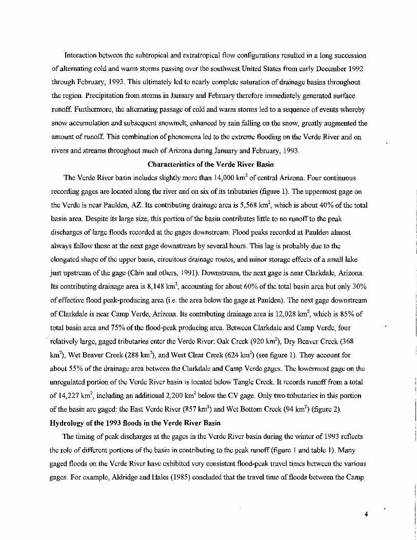
Contributing Discharge Unit
Site Name Discharge Area (km2
) ( m3/s) ( m3/s/km 2
)
Gages Verde River near Camp Verde (CV) 12,028 1,416 0.12
Verde River below Tangle Creek (TC) 14,227 4,106 0.29
East Verde River 857 569 0.66
Wet Bottom Creek 94 209 2.22
Paleoflood Red Creek (RC) 13,683
Reaches - -Ely-Baker (EB) 13,932 3,682 0.26
Miscellaneous Red Creek 128
Sites - -Horse Creek 32 - -
Sub-Basins CV-TC 2,167 2,690 1.24
TC-EB 264 425 1.61
Table 2. Contributing areas, peak discharges, and unit discharges for the January flood at various sites in the lower Verde River basin.

1 2 4106 4106
4,000 -- ------------------- ------- -------- --------------------------- ____ B__ 4,000
"'C c:: o o Q) tJ)
3 3440
4
1'47' 3130
5
13313
3130
7
6 f70 1
3653 3450
3370 3282
03 3,000---- ------------- __ B _____________________ B __ B_________ - ----- - - ----- _________ B__ ______________ BB _____ _ ------- 3,000 c:L 2975
~ Q)
1i> E o .c ::::J o c:: Q)
e> 2,000 CO
.c:: o tJ)
o
1,000
1416
2478
1) Peak discharge estimates for the early January 8 flood peak at Camp Verde (CV) and Tangle Creek (TC) gages.
2) Peak discharge estimates for January 8 at CV (1 PM) and TC (8:30 AM) .
3) Maximum: TC peak minus unit discharge from the area between CV and TC applied to the area between TC and Red Creek (RC);
Minimum: TC peak minus unit discharge of Wet Bottom Creek (WBC) applied to all of the drainage area between TC and RC.
4) Max: Estimated peak discharge at the Ely-Baker (EB) site minus WBC peak;
Min: Estimated peak discharge at EB site minus unit discharge ofWBC applied to the rest of the drainage area between EB and RC sites.
5) Max: Estimated peak discharge at EB site minus WBC peak minus unit discharge of lower Verde basin applied to the rest of the drainage area between EB and RC sites;
Min: Estimated peak discharge at EB minus WBC peak minus WBC unit discharge applied to the rest of the drainage area between EB and RC sites.
6) Peak discharges reported for the February 20 flood at CV and TC.
7) Step-backwater modeling of the highest flotsam, varying Manning's n from 0.04 to 0.035; "X" marks the preferred discharge estimate using n = 0.0375.
Figure 4. Constraints on the peak 1993 discharge at the Red Creek study reach.


TC and RC, then a likely minimum discharge estimate of 2,975 m3 S·l (105,000 cfs) results. Thus, using
only the gage data, the estimated range for the January discharge through RC is 2,975 to 3,440 m3 S·l.
We obtained an independent estimate from the Ely-Baker reach that can be used to further constrain the
discharge at the Red Creek site. At this site we estimated the 1993 flood peak discharge as 3680 m3 S·l
(130,000 cfs) by reoccupying a cross section (section 9) and comparing the elevation of flotsam to stage
discharge relations reported in Ely (1985) and Ely and Baker (1985). In their study they reported an
estimate for the 1980 flood discharge that was consistent with the gage estimate (i.e. within 1 %), thus we
assume that our estimate for the 1993 peak from this reach is reasonably good. Since the Ely-Baker site is
located below the mouth of Wet Bottom Creek the difference between their peak discharges, 3,475 m3 S·l
(122,620 cfs), is a reasonable maximum bounding value. Again, we claim that this is a maximum because
it assumes no input from Red Creek which also enters the river between the study sites. A minimum of
3,130 m3 S·l (110,540 cfs) results from the difference between the Ely-Baker estimate and the unit
discharge ofWBC applied to the area between the Ely-Baker and Red Creek sites (249 km2). This range
can be narrowed further by limiting the application of unit discharges to only the Red Creek basin (128
km2). An upper limit of3,313 m3
S·l (117,000 cfs) results from applying the unit discharge of the area
between CV and TC; and a lower limit results from applying the Wet Bottom Creek unit discharge. We
conclude that the peak discharge of the January flood through the Red Creek reach was probably between
3,130 and 3,313 m3 S·l.
The Late February Flood. In the late February flood, peak discharge on the Verde River increased
from 3,370 m3 S·l at CV to only 3,653 m3
S·l at TC, so approximately 95% of the peak originated upstream
of the CV gage. This indicates that the February peak through the Red Creek reach has a lower limit (3,370
m3 S·l) greater than the upper limit of the likely range of the January peak discharge (3,313 m3
S·l) (figure
4). Thus, we conclude that the February flood was probably the larger peak through the Red Creek reach.
The tremendous increase in the discharge of the early January flood in the lower basin was such that the
peak discharge was less than the February peak through a significant length of the river between CV and
TC, but was 565 m3 S·l (20,000 cfs) larger by the time it reached TC. The Red Creek reach is probably just
upstream of the cross-over point where the two peaks were the same. Because both Red and Wet Bottom
creeks enter the Verde between the Red Creek and Ely-Baker reaches, the January flood was probably
larger than the February flood in the latter reach.
In our field investigations we did not note any conclusive evidence for the passage of two floods
through the Red Creek reach, suggesting that evidence from the first flood was obscured by the second,
7

slightly larger flood. Evidence oftwo floods at the Ely-Baker reach is subtle because the peak stage of the
January flood was probably less than 30 cm higher than the February flood. This small difference should
have resulted in the flotsam from the February flood being deposited on the surface of January flood
sediment. We observed this relationship in the field, but at that time we interpreted it to be the result of
deposition during recession ofthe January peak.
Paleoflood Methodology
Paleoflood hydrology generally refers to the study of floods that occurred in the absence of
instrumental observation or historical documentation (Baker, 1987, 1989). However, the term is also
appropriate for the application of the same methodological procedures to studies of modem or historical
floods (e.g. House and Pearthree, in press). A primary value of paleoflood studies is the extension of flood
records by hundreds to thousands of years. Documentation of the actual occurrences of extreme floods over
this time frame has important applications to studies of climatic variability (Ely and others, 1993), long
term flood magnitude-frequency characteristics (O'Connor and others, 1994), and potential bounds on
flood peak magnitudes (Enzel and others, 1993).
In our study, we used the slackwater deposit-paleostage indicator (SWD-PSI) method of paleoflood
reconstruction because it has proven to produce the most accurate estimates of paleoflood magnitudes
(Baker, 1989). The SWD-PSI method estimates peak discharge through comparison of relict high-water
indicators (SWD and PSI) to water-surface profiles generated from a step-backwater model such as HEC-2
(Hydrologic Engineering Center, 1985). The method is best suited for bedrock canyons or otherwise stable
channels which are conducive to long-term preservation of flood evidence that retains a direct relation to
the pre-flood and post-flood channel geometry (Baker and Kochel, 1988). Also, stable channels are
generally more realistically characterized in hydraulic modeling. In a typical SWD-PSI study a range of
discharges is reported from a visual assessment of the best overall agreement between the model-predicted
profile and the relict high-water indicators (O'Connor and Webb, 1988).
Slackwater deposits (SWD) are sedimentary flood deposits usually consisting of silt, sand, and
occasionally gravel that accumulate in areas of reduced flow velocity during floods (Kochel and Baker,
1988). SWD provide minimum estimates ofthe associated peak flood-stage because they are deposited at
some depth below the peak water surface. Paleostage indicators (PSI) include a variety of non-sedimentary
types of flood evidence, including: flotsam, scars on vegetation, erosion marks on canyon walls, flood
related vegetation distributions, and evidence for non-inundation. The relation between the elevation of a
PSI and the associated peak flood-stage is variable and depends on the nature ofthe indicator. For example,
highest flotsam commonly corresponds closely to peak stage, but flood scars on vegetation and/or canyon
8
walls, and massive piles offlood debris vary in their relation to peak stage. More detailed explanations of
the SWD-PSI method can be found in: Baker (1987); Kochel (1988); Kochel and Baker (1988); O'Connor
and Webb (1988); and Baker (1989).
The SWD-PSI method is similar to other indirect methods of estimating peak discharges of recent
floods (e.g. Benson and Dalrymple 1967; Dalrymple and Benson, 1967). An important difference, however,
is the use of step-backwater modeling instead of the slope-area method, which is commonly used in indirect
estimates of recent large floods at ungaged sites and extension of rating-curves at gaged sites. The different
choice of models reflects uncertainties inherent in the paleoflood evidence. Slope-area modeling requires a
water-surface profile specified by high-water marks (e.g. flotsam), channel geometry, and energy-loss
coefficients to calculate the discharge. In contrast, the step-backwater method treats discharge as a known
value and uses it in conjunction with channel geometry and energy-loss coefficients to calculate the water
surface profile. This method is a logical choice for paleoflood studies where the true water-surface profile
is often not precisely known from the basis of the relict stage indicators, but the channel geometry is
reasonably well-constrained. In our re-study of the Verde River, even though definitive peak stage
indicators were present, we used step-backwater modeling to facilitate comparison with previous studies
and evaluate uncertainties in paleoflood reconstructions in general.
Limiting assumptions of the SWD-PSI method are associated with the flow model and its application in
the context of paleoflood hydrology. Principal assumptions include: (1) flow is steady, gradually varied,
and one dimensional; (2) channel cross-section boundaries are stable; (3) energy slope is uniform between
cross-sections; (4) cross-section characteristics and the estimated energy loss coefficients are representative
of those affected by the flood(s) in question; (5) PSI approximate the stage of the flood(s) in question
slackwater deposits represent a minimum peak flood-stage, but other types of paleostage indicators may
represent the peak water surface (flotsam), or provide a maximum bound on the peak stage (e.g. some flood
scars, or evidence of non-inundation); and (6) either a negligible amount of scour or deposition has
occurred in the channel during and since the flood peak, or any that occurred can be accounted for in some
way (modified from O'Connor and Webb, 1988; Hoggan, 1989; and Baker, 1989). These assumptions
apply to most types of indirect discharge estimation, but their relative importance increases with the
amount of time between the occurrence of the flood(s) and the reconstruction attempts. Focusing modeling
efforts in stable channels helps to minimize the violation of some of the assumptions and the effects of time
variant changes in channel geometry.
9

Field Investigations
In our study following the 1993 floods, we resurveyed a 500-m-Iong stretch ofthe Verde River that
constitutes the lower third of the Red Creek reach studied previously by O'Connor and others (1986). Our
field investigation was performed in June, 1993, approximately 4 months after the flooding. The study
reach is in a relatively wide canyon with steep to nearly vertical walls. Bedrock protrudes from the bed at
several places along the canyon bottom, elsewhere, the bottom is composed of a pool and riffle sequence
with an average slope of about 1 percent. Much of the canyon bottom area above the perennial low flow
channel consists of a nearly flat boulder and cobble bar. The alluvial cover throughout the reach is
probably thin; however, depth to bedrock was not determined quantitatively.
Our study reach consists of nine cross sections within a 500-m-Iong stretch of the canyon with an
average width of 110m. A topographic survey was performed with a total station survey instrument and
several hundred points were collected to define the canyon topography and precise locations of
approximately 50 different stage indicators. Deposits from the 1993 floods were easily identified by the
lack of seasonal vegetation rooted in the sediment, unconformable relations to vegetation rooted in lower
SWD, and an overall fresh appearance. SWD from 1993 overlay the all of the SWD described by
O'Connor et al (1986), but were inset into and about 1.5 m below the top of the highest SWD that were
identified during this survey of the reach. We observed that canyon expansion areas have the most
extensive SWD; however, the sites with the thickest and highest deposits are small, protected alcoves along
the margins of the flood flow
Types of High-water Marks Used in This Study
In the interest of developing a data set relating to most paleoflood studies we surveyed three types of
flood stage indicators: flotsam, uppermost "edges" of slackwater deposits (ESWD), and the relatively flat
"tops" of massive slackwater deposits (TSWD) (see figure 5, for example).
Flotsam includes any type of obviously floated delicate, organic material. In quiet-water areas along
the margins of flow, flotsam deposits usually consisted of delicate organic material like small twigs and
mats of leaves. At the very edge of inundation, flotsam was commonly deposited in fairly narrow,
curvilinear arrangements conforming to the contours of the local topography. The 1993 flotsam along the
perimeter of the reach was abundant, readily identifiable, and the highest points that we surveyed clearly
represented the limit of inundation at that point. Delicate flotsam lines are the best indicators of the peak
water surface, but their long-term preservation potential is poor.
We define the edge of a slackwater deposit (ESWD) as the uppermost elevation of the thin tapering
"landward" edge of the deposit. During our survey, ESWD were often observed as thin drapes offresh
10

Discharge Range from rating curve
(n: 0.04-0.036)
3843-4211
3441-3782
3240-3564
2916-3222
2787-3085
2500-2777
2433-2700
Adjusted range
4996-5474a
4473-4917a
3240-3564b
3791-4188a
3240-3564c
3240-3564a
3163-3510a
Elevation (m)
984.74
984.32
984.10
983.74
983.59
983.20
983.14
a. 30% correction applied
?
EXPLANATION Unit 1: -1000 BP
Unit 2: >1000 BP
Unit 3: 1891?
Unit 4: >1000 BP
Unit 5: 1993
:'~\4III--- 93 Flotsam
--- Edge 93 SWD
bottom of trench ? ?
b. no correction applied--diagnostic indicator c. 16% correction applied for equivalence with flotsam estimate
Figure 5, Stratigraphic section and peak discharge estimates using a rating curve developed for section 7 of the Red Creek study reach. Discharge estimates in the left column are obtained directly from stage of the deposit and the associated discharge, Adjusted discharge estimates account for the underestimation of peak stage associated with slackwater deposits in this reach. No correction is applied to the 1993 flotsam-based discharge estimate.


sediment over hillslope colluvium or bedrock on the canyon margin. ESWD elevations were quite variable
throughout the reach. Some tapered out at delicate flotsam lines, indicating deposition up to the water
surface, but more often they were between the highest flotsam and the tops of the slackwater deposits.
ESWD are important because they represent the highest level of sedimentation associated with a flood.
However, their preservation potential is only poor to moderate because the layer of sediment is typically
quite thin.
The tops of slackwater deposits (TSWD) are the most important and long-lived flood-related
sedimentary features we observed. We define TSWD as the relatively flat surfaces on top of thick
accumulations of slackwater sediment. An important distinction between TSWD and ESWD is the
thickness of the underlying sediment. At each TSWD point it would have been possible to excavate and
examine stratigraphy of the underlying deposit, whereas most of the ESWD points were just thin drapes of
sediment (em to mm). TSWD sites are much more likely to persist over long periods oftime (lOOs to 1000s
of years) than are the more ephemeral flotsam deposits and ESWD, and thus we conclude that they are
representative of most SWD examined in paleoflood studies.
Hydraulic Modeling of the Red Creek Reach
In most paleoflood studies, flow modeling is typically a multi-stepped, trial and error procedure
involving many variations in the initial water surface elevation, discharge, and channel roughness values.
Each of these variables is either unknown or poorly constrained in a typical paleoflood study; however, in
our study the initial condition of the starting water surface elevation was known due to the presence of
many definitive HWMs, and our selection of appropriate n values was controlled by the constraints on the
peak discharge previously described.
We contend that the February flood was most likely the largest to pass through the Red Creek reach
during the winter of 1993, although the January peak was larger downstream at the TC gage; therefore, the
peak discharge was probably between 3,370 m3 S-1 and 3,512 m3
S-I. In modeling the Red Creek reach, we
found that the discharges associated with composite Manning's roughness coefficients (n) of 0.035 and
0.04 are 3,700 m3 S-1 and 3,300 m3
S-1 respectively, which effectively bracket the assumed "actual" peak
discharge. The intermediate n-value of 0.0375 resulted in an estimate of3,450 m3 S-1 (figure 6), so this n
value is probably representative of the reach. The predicted water surface profile agrees well with the
highest flotsam throughout the reach.
We visually fit water-surface profiles to the two other types of high-water indicators of interest in this
study (ESWD and TSWD) in order to evaluate the discharge estimates associated with the highest points in
each category (figure 6). In these modeling runs we altered the treatment of the initial conditions because of
11

~ Q)
986
984
Q) 982 E
§ 980
~ iii 978
ill
ft' • . ... ... ... ..
Distance upstream, meters
• Flotsam
V Edge ofSWD
... Top ofSWD
Figure 6. Example of the use of step-backwater modeling to visually estimate discharges associated with various types of water-surface indicators from the Red Creek reach. Profiles shown correspond to modeling with composite n = 0.0375. Cross section locations are numbered.

.... 'Ill
4000
3500
ME 3000
oj e' ca
13 2500 III
is
2000
1500
-
-
Flotsam n = 25
~
'-~I-j;t:
I I I I
to to "'I' ..., I"- 0 0 ..., 0 0 0
0
ESVVD n = 11
I
I-~ I
IX
I I-
L;
I I I
to to "'I' ..., ,... 0 0 ..., 0 0 0
0
Manning's n
TSVVD n = 19
lir l-
ll< x , I
I I
to to "'I' ..., ,... 0 0 ..., 0 0 0
0
75"10
x= mean 50"10
25%
10"10
Figure 7. Box plot showing the discharge estimates associated. with flotsam, edges of slackwater deposits, and tops ofslackwater deposits. The effect of varying Manning's n values are also illustrated. Percentile boundaries of data sets shown in legend.
Flotsam ESWD TSWD
0.035 0.0375 0.04 0.035 0.0375 0.04 0.035 0.0375 0.04
Mean 3211 3035 2873 2908 2741 2590 2450 2311 2185
Std.Oev. 350 335 322 374 359 343 270 258 245
Max. 3669 3444 3282 3370 3178 3024 3029 2823 2647
Min. 2425 2270 2136 2378 2254 2143 1995 1887 1788
Table 3. Comparison of discharge estimates for various types of stage indicators using a range of Manning's n values.

The relative distribution of the point-rating discharge estimates are generally consistent with the visual
discharge estimates. The highest flotsam corresponds to the highest discharges, TSWD to the lowest
discharges, and ESWD to intermediate values. The variability in the estimates from each type of indicator
reflects uncertainties faced in any attempt to indirectly estimate the peak discharges of large floods because
ofthe complex, multi-dimensional nature of flooding. Flotsam was identified at various levels in the reach,
suggesting that relatively steady conditions may have prevailed at various times during the waning of the
floods and/or the flotsam deposits may have been emplaced randomly as the flood stage decreased.
Variability of the SWD elevations may reflect a similar waning-stage phenomenon, but deposition could
occur simultaneously at different levels in different settings depending on local geometric constraints
(Kochel and Baker, 1988). These factors reinforce the importance offocusing on the trends of the highest
indicators of each category when estimating peak discharges.
The most conservative peak discharge estimates are those associated with the highest elevations from
each indicator category. The following ranges correspond to composite n values of 0.04 and 0.035,
respectively. The range of the maximum flotsam estimate is 3282-3670 m3 S-I; the range of the maximum
ESWD estimate is 3024-3370 m3 S-1; and the maximum TSWD estimate is 2647-3029 m3
S-1. Ifa typical
paleoflood study were conducted at the Red Creek site several decades hence, researchers would likely
establish a peak discharge estimate corresponding to the maximum TSWD estimate obtained in our study.
This would, of course, constitute a minimum estimate. The SWD-based underestimation expressed in this
data set ranges from 22% to as much as 49%, based on comparing the maximum FLT estimate to the
maximum and average TSWD estimates, respectively. The percentage differences between the variety of
indicators is outlined in table 4.
We believe that bracketing the HWMs between successive profiles or simply enveloping the highest
indicators with an individual profile are reasonable techniques for discharge estimation in the context of
paleofloods, historical floods, and recent large floods given the variety of potential uncertainties in each
case. The point rating technique is illustrated here simply as a convenient means of precisely determining
the limits of the bracketing discharges and, in this sense, is superior to specifying a discharge range simply
from the basis of a visual assessment.
Cross-Section Rating Discharge Estimates
The development of a rating curve at an individual cross section following the formulation of a
successful modeling scenario of an entire reach is another method for discharge estimation commonly
employed in paleoflood studies. Rating curves are useful at sites where a stratigraphic exposure of
paleoflood deposits is located. In our study, cross-section 7 contains both the variety of 1993 high-water
13
greater uncertainty in the appropriate starting water-surface elevation. The HEC-2 program has an option
to calculate the initial water-surface elevation using a slope-area calculation. In this procedure, the user
provides an estimated starting elevation, a "known" discharge, and a "known" energy gradient. The
program first calculates a water surface elevation that balances with the "known" parameters through an
iterative procedure. Once the balance is obtained, the computations proceed through the reach. We used the
water surface slope measured from flotsam at the downstream end of the reach to represent the energy
gradient in our attempts to model profiles consistent with the ESWD and TSWD points. In these additional
modeling scenarios, we retained the composite n value range of 0.035-0.04.
Point-Rating Estimates of Discharge
Most previous SWD-PSI paleoflood studies have relied on bracketing SWD and PSI between
successive water-surface profiles to estimate a range of associated peak discharges; thus the basis for the
reported discharge or range of discharges is visual (O'Connor and Webb, 1988). This technique is
generally adequate given the variety of uncertainties in indirect discharge estimation of large flood
discharges; however, it does not necessarily provide detailed information about the actual spread of
discharges associated with individual stage indicators, which is a principal goal of our study. In addressing
this, we adopted a method that assigns specific discharge values to each individual stage indicator in the
reach. This approach, which we have termed the "point-rating" method involves a more rigorous evaluation
of model output and allows for a more precise evaluation of the spread of the associated discharge
estimates, a more direct comparison of estimates from flotsam and slackwater deposits, and a better
evaluation of stage indicators located between cross sections.
Placement of the SWD and PSI along the longitudinal profile of the channel in the correct position for
comparison to the estimated water-surface profiles can be a subjective and potentially arbitrary procedure,
particularly on large streams. In developing the point-ratings we adopted a set of simple, linear equations to
make this and the determination of discharge more accurate and systematic. First, the mid-channel profile
was divided into straight subreaches and the stage indicators within each sub-reach were then projected
along a line perpendicular to the mid channel line. The elevation and distance from the downstream end of
the reach were used to precisely locate each point in its proper position along the profile. A set of simple
linear equations was used to determine the elevation corresponding to each point's longitudinal position on
bracketing water-surface profiles separated by 200 m3 S·l increments, and another linear relation determined
the discharge at the point's vertical position by defining the stage-discharge relation at its longitudinal
position. This method was applied to the results of modeling scenarios using n values of 0.035, 0.0375, and
0.04. The results are summarized in table 3 and figure 7.
12

Peak discharge estimates (m3 S-1)
Point-Rating Analysis Rating Curve
Indicator Type Min Mean Max Max
TSWD 1887 2311 2823 2646 ESWD 2254 2741 3178 2939 FLT 2270 3035 3444 3400
Percentage difference between discharge estimates
(relative to max. flotsam estimate)
FLTandTSWD 82.5 49.0 22.0 28.5 FLTand ESWD 52.8 25.6 8.4 15.7
Table 4. Comparison of the differences between discharge estimates based on SWD and flotsam using the point-rating method and a .ratingcurve for one section.

marks and an exposure of SWD stratigraphy that records at least 4 large floods prior to 1993 (figure 5).
The highest slackwater deposits identified at this site are approximately 1.5 m higher than the highest
deposits identified by O'Connor et al (1986). The capping deposit is probably correlative with the 1000
year BP paleoflood described at the Ely-Baker reach (Ely and Baker, 1985).
The discharges associated with the different types of indicators in section 7 from the 1993 flooding are
as follows, assuming n values of 0.035 and 0.04: flotsam, 3240-3564; ESWD, 2737-3085; and TSWD,
2500-2777. Using the average values from each range, the measures of SWD-based underestimation are
18% (flotsam and ESWD) and 30% (flotsam and TSWD). These results are consistent with the estimates
based on the point-rating of the entire reach. The maximum difference in the peak discharge estimated from
flotsam in the point-rating method and the section rating method is only 3 %. Differences in the maximum
discharge estimates reflect variability inherent to the nature of the data.
Section Rating Estimates from the Ely-Baker Reach
We observed that SWD and flotsam can have considerably less vertical separation in areas where the
confining slope is less steep. At a site in the Ely-Baker reach downstream, we assessed the SWD-based
underestimation in addition to the flotsam-based peak discharge estimate described previously. At this site
there was a relatively small difference between the elevations of the highest flotsam and TSWD (~30 em).
The discharge corresponding to the flotsam was 3680 m3 S-1 (130,000 :fi? S-1), and the discharge
corresponding to the TSWD was 3500 m3 S-1 (123,600 fe S-1). The associated SWD underestimation factor
is thus only about 5%. We hypothesize that the smaller difference in flotsam and TSWD-based discharge
estimates is controlled by the geometry ofthe depositional site, which is a broad embayment at the mouth
of a small tributary. The more gradual slope of this site and the greater width of the river were apparently
conducive to sedimentation up to level very near the peak water surface in the sense that the "top" and
"edge" of the deposit were essentially the same thing. This small difference may explain in part why the
modeling results reported by Ely and Baker (1985) from this reach were consistent with the TC gage
estimates. Their discharge estimate for the 1980 flood was within 1 % of the gage estimate, and their
estimate for the 1951 flood was within 15% of the gage estimate. The 1980 estimate was based on flotsam,
whereas the 1951 estimate was based on SWD.
Evaluation of Results
The whole-reach (point-rating) and single-site rating approaches produced maximum peak discharge
estimates that differ by only 3 %. Estimates of SWD-based underestimation are also similar. Based on the
point-rating data, the underestimation factor ranges from 22-49% (based on difference in maximum and
average values respectively); and using the single-section rating curve the factor was 30%. Given that the
14

highest indicator in a given category would be sought in a paleoflood study at this site, we believe that 30%
is a reasonable, conservative measure. The amount of underestimation is controlled in part by the general
geometry of the depositional environments typical of this reach and probably varies as a function of flood
stage. The 5% underestimation factor from the Ely-Baker reach illustrates the effect of depositional
environment. In general the highest slackwater deposits on the Red Creek reach are in small, protected
alcoves along the channel margins. At these sites, the edges of the depositional areas are confined by steep
canyon walls which apparently constrained the vertical limit of sedimentation to an average depth of about
1 m below the water surface. The site we investigated in the Ely-Baker reach was a gently sloping bench of
sediment in a tributary embayment, and the cross-section was wider than any in the Red Creek reach. Here,
the difference in elevation between SWD and flotsam was only 30 cm.
Discussion - Reconciliation of Discharge Estimates for Verde River Floods
The original study at the Red Creek reach by O'Connor and others (1986) was performed as an
independent test ofthe reproducibility of the results described by Ely and Baker (1985). They concluded
that their results confirmed the flood chronology and relative flood magnitudes reported by Ely and Baker
(1985), but their discharge estimates for assumed correlative flood deposits were considerably lower and
the 1,000 year BP flood deposit was not identified. O'Connor and others (1986) concluded that much of the
discrepancy was from differences in drainage area and the fidelity of the SWD elevations to the peak water
surface at each site. Our restudy of the Red Creek reach confirms the importance of these factors by
documenting the magnitude of their influence on peak discharge estimates. In addition, we found evidence
for what we believe is the 1,000 year BP flood, and we have an alternative interpretation ofthe deposits
likely associated with historical floods that is more consistent with the Ely-Baker reach and the gage. Each
of these factors, SWD-based underestimation, contributing drainage area differences, and new stratigraphic
evidence, is critical in reconciling the differences between the discharge estimates from the two paleoflood
study sites and the TC gage.
SWD-based Underestimation
The effect of SWD-based underestimation is an obvious control on large differences in paleoflood
estimates from disparate sites. This phenomenon is particularly critical in comparisons of SWD-based
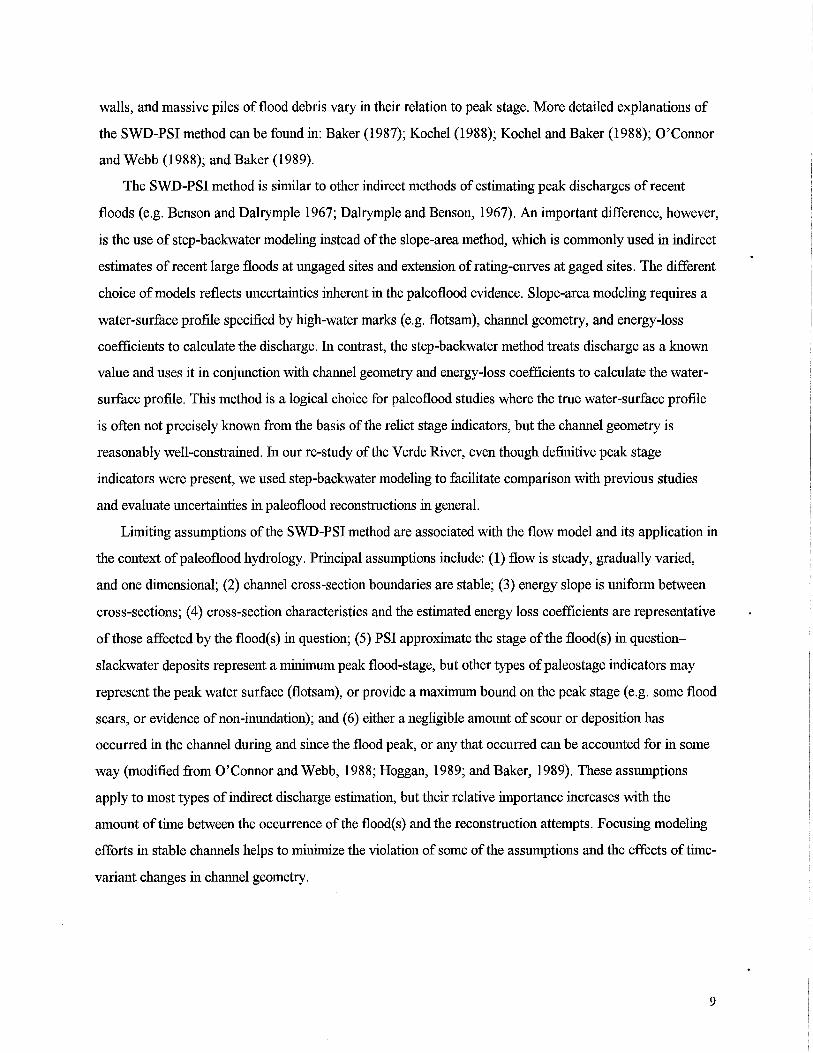
estimates to similar estimates from diverse settings and to gaged estimates. Discharge estimates for flood
peaks in excess of 1,000 m3 S-1 on the Verde River from paleoflood studies and gaging stations are depicted
in figure 8 (see also tables 5 and 6). Estimates from the Red Creek reach and the Ely-Baker reach are
shown as ranges. The lower end of the range corresponds to the maximum reported, SWD-based estimates
for the given flood or series of floods. The upper limit corresponds to that value adjusted by the
15
-"0 C 0 C) CD In ... CD a. ~ CD -CD E C)
:.a :J C) -CD e» C'IJ .c C)
.!!! C ~
C'IJ CD a..
1000 BP
1000 BP
5,000 5,000
4,000 4,000 1
993
1993 993b
938 3,000 3,000
1938 1
1993a 1978b
978b
2,000 2,000 978a 916
1972 1951 970
I 1966
1,000 '---=""---------""'"'------------'~----- '---------~----' 1,000 Red
Creek Ely-Baker
reach Tangle Creek
Camp Verde
12,030 km 2
below E. Verde
13,615 km 2 13,703 km 2 13,952 km2 14,227 km2
Figure 8. Summary diagram of gaged, historical, and paleoflood peak discharge estimates for the lower Verde River. Total drainage area to each site is shown. The gage record is longest for Tangle Creek and its predecessors; the Camp Verde record begins in 1936, and only a few large floods were recorded at the now defunct gage near the E. Verde River confluence. Paleoflood estimates from the Red Creek and Ely-Baker reaches are shown as ranges, with a x marking the preferred estimate. They are based on our 1993 field s tudies and upward adjustment of previous paleoflood discharge estimates from Ely and Baker (1985) and O'Connor et al (1986), based on our recent work.


Comparison of discharges from sites along the lower Verde River: gaging stations
Near Camp Below East Below Verde Verde Tangle Ck.
Year Month Day (09506000) note (09508000) note (09508500)
1995 3 6 2,138 a - 2,543
1995 2 15 2,022 a - 3,059
1993 2 20 3,370 h - 3,512
1993 1 8 2,478 hJ - 4,106
1980 2 20 1,589 b,G - 1,863
1980 2 15 1,753 b,G - 2,685
1978 12 19 2,192 b,G 2,249 9 2,662
1978 3 1 1,552 b,G 1,914 f 2,588
1972 10 20 1,150 b,G - 1,795
1970 9 5-6 1,247 b,b - 1,753
1966 12 7 - - 1,501
1951 12 31 - - 2,311
1941 3 14 850 e 1,408 d 1,240
1938 3 3-4 2,747 e 3,115 d 2,832
1937 2 7 1,181 d,e 1,943 d 1,784
1932 2 9 - - 1,501
1927 2 17 - - 1,982
1920 2 22 - - 2,690
1916 1 20 - - 1,951
1905 11 27 - - 2,719
1891 2 24 - - 4,248
Notes
a. provisional data provided by USGS
b. discharge recorded at gage #09505550, "below Camp Verde", value in table includes peak from
West Clear Creek (station 09505800) for comparison to values from station 09506000
c. Chin, Aldridge, and Longfield, 1991
d. Patterson and Somers, 1966
e. Garrett and Gellenbeck, 1991
f. Aldridge and Eychaner, 1984
g. Aldridge and Hales, 1984 h. USGS, Water Resources Data, Arizona, Water Year 1993
i. only 57% of peak contributed to peak at Tangle Creek gage
note
a
a
h
h
G
e
e
e
e
e
e
d,e
d,e
d,e
d,e
d,e
d,e
e
d,e
d,e
d,e
Table 5. Summary of discharge estimates for large historical floods at gaged sites on the lower Verde River. See Patterson and Somers (1966) for gage histories.


Comparison of discharges from sites along the lower Verde River: paleoflood study sites
Red Creek Reach Ely-Baker Reach
Date Reported Adjusted (30%) Reported Adjusted (5%) min max min max notes min max min max notes
1993 3282 3664 a 3500 3680 e
1980 1800 2000 2340 2600 b 2700 2700 2835 d
1978b 1700 2000 2210 2600 b
1978a 1400 1700 1820 2210 b
1951 1200 1400 1560 1820 b 1950 1950 2048 d
1938 2000 2200 2600 2860 b,c
1920 2000 2200 2600 2860 b,c
1905 2000 2200 2600 2860 b,c
1891 2916 3222 3791 4188 c,f,g 3500 3800 3675 3990 f
1000 BP 3843 4211 4995 5474 c,f,g 5000 5400 5250 5670 f
Notes
a. range from this study associated with highest flotsam and range of Manning's n: 0.035 - 0.04
b. reported ranges based on examination of water-surface profile and SWD comparisons in O'Connor et al. (1986)
c. value corresponds to indentification and/or reinterpretation of SWD stratigraphy from this study
d. reported range corresponds to single value reported in Ely and Baker (1985) and equivalent adjusted values
e. range corresponds to discharge estimate from TSWD and Flotsam
f. range corresponds to TSWD estimate and adjusted equivalent
g. range corresponds to TSWD estimates from rating curve (n: 0.035 - 0.04) and equivalent adjusted values
Table 6. Comparison of paleoflood discharge estimates from the Red Creek and Ely-Baker reaches on the Verde River. Reported values are from the original studies; adjusted values reflect corrections for SWD-based underestimation determined in this study.


underestimation factors derived in our study (table 6). Clearly, accounting for underestimation has a
significant effect on the comparison and reduces the apparent discrepancy considerably.
Contributing Drainage Area
Consideration of the influence of drainage area provides further reinforcement for the consistency of
the record throughout the basin. Peak discharges for virtually every flood in the gage record increase with
increasing drainage area in the lower Verde basin. The only exception is the 1938 flood discharge. The
1993 floods provided very dramatic examples of the variable influence of increasing drainage area on peak
discharges. In the January 1993 flood the discharge nearly tripled between CV and TC, while the February
1993 flood underwent a negligible increase. As shown in figure 8, the January event is the most extreme
example of discharge increasing downstream in the systematic record. Several other floods behaved like the
February 1993 flood, but most floods showed gradual increases in peak discharge with increasing drainage
area. Relatively minor differences in contributing drainage area can have a large effect on peak discharge
estimates from sites that are relatively close together if these sites happen to be along a reach that received
substantial tributary input.
Paleoflood Stratigraphy
Our identification and interpretation of the SWD sequence in section 7 of the Red Creek reach offers a
final element to the reconciliation of the discharge estimates from the various sites. It also extends the
paleoflood record preserved in the Red Creek reach and helps to clarifY uncertainty concerning the 1938
and 1891 floods as interpreted in the previous paleoflood study at the Red Creek site.
The newly discovered stratigraphic exposure at cross section 7 of the Red Creek reach reveals evidence
for at least two paleofloods larger than the 1993 event that are probably 1,000 years old or more (see figure
5). We tentatively correlate the highest deposit with the uppermost deposit of the Ely-Baker reach, whose
age has been constrained to 1,000 years BP by a 14C date ofin situ charcoal and diagnostic Hohokam
artifacts found on the surface of the deposit (Ely and Baker, 1985). The correlation is based on relative
topographic positions of the deposits and the discharge estimates associated with them. We identified
similarly high and probably correlative flood deposits at four other sites in the Red Creek reach. The
discharge at section 7 that corresponds to the highest deposits is 5000-5474 m3 S-I (176,700-193,300 cfs).
The maximum adjusted point-rating estimate from a likely correlative, but slightly higher deposit at another
site in the reach is 5405-6200 m3 S-I (190,875-219,000 cfs). The adjusted estimate from the Ely-Baker
reach is 5940 m3 S-I (210,000 cfs). The underlying flood deposits (units 2 and 4) obviously predate unit 1,
but the lack of any direct numerical control on these units precludes any specific age estimate for the
associated floods.
16

The flood deposit that is inset below these deposits but above the highest 1993 flood deposit (unit 3 in
figure 5) may have been emplaced by the 1891 flood. The peak discharge of this flood above the confluence
of the Verde and Salt rivers was estimated as about 4,200 m3 S-1 (150,000 cfs; Patterson and Somers,
1966). Ely and Baker (1985) identified a likely 1891 SWD in their reach that corresponds to an adjusted
discharge estimate of 4180 m3 S-1 (147,600 cfs). In the Red Creek reach, O'Connor et al (1986) interpreted
a considerably lower SWD as corresponding to the 1891 flood. The adjusted discharge estimate for this
SWD is approximately 3100 m3 S-1 (109,500 cfs). This difference is implies a larger increase between the
Red Creek and Ely-Baker sites than the January 1993 flood. This is possible; but, we think that it is more
likely that this deposit is from the 1938 flood. This event had peak discharges of 3100 m3 S-1 at the gage
below the Verde - East Verde river confluence (figure 2) and 2800 m3 S-1 at a site about 10 km downstream
from the present TC gage. Assuming that these gaged peaks are reasonably accurate, then at the Red Creek
site the peak discharge would have been in the range of the 1891 flood discharge estimated by O'Connor
and others (1986). The 1938 flood deposits were probably buried by the 1993 floods. If this scenario is
correct, then the adjusted discharge estimates for the 1891 flood at the Red Creek and Ely-Baker reaches
are 3790-4200 m3 S-1 (133,900-148,300 cfs) and 4180 m3 s-I(147,600 cfs), respectively.
The scenario outlined above reconciles the gaged, historical, and paleoflood data quite well, but in the
absence of better numerical age constraints on the various flood deposits it remains somewhat speculative.
If the high inset deposit shown in figure 5 is not an 1891 flood deposit, then the 1891 flood at Red Creek
was evidently smaller that the 1993 flood and the associated SWD are buried. In this less likely scenario,
the high inset deposit represents a flood that occurred sometime between 1,000 years BP and 1891, and the
location of the 1938 deposit is unresolved.
Stratigraphic Implications of the Complex Flood Record
The potentially large influence of drainage area on peak discharge in a small portion of the Verde River
basin reveals potential complexities in the hydrology of extreme floods on the Verde River (i.e. those
involving large runoff contributions from much of the basin). The corresponding stratigraphic record of
flooding at disparate sites would reflect this. Our approach to reconciliation was useful in interpreting the
largest floods at each site but it relied heavily on gage data. Detailed correlation of a more complete
paleoflood chronology incorporating higher frequency events from several sites would be a daunting
challenge.
A complicating factor results from the fact that variations in the relative contribution of runoff from the
middle and lower parts of the Verde basin in different floods caused the relative magnitude of some floods
to be inverted between CV and TC and sites between them. In fact, we believe that the cross-over point was
17

between the Red Creek and Ely-Baker reaches in the 1993 floods. The recent flood history ofthe lower
Verde River has two additional examples of this phenomenon occurring in years in which two large flood
peaks occurred (1980, 1993, 1995). As illustrated in figure 8, the relative ranking oflarge gaged floods at
CV, in order of decreasing size, is Feb. 1993, 1938, Jan. 1993, Dec. 1978, Mar. 1995, Feb. 1995, 1980,
and Mar. 1978. At TC the relative ranking is Jan. 1993, Feb. 1993, Feb. 1995, 1938, 1980, Dec. 1978,
Mar 1978, and Mar. 1995. Note that the differences between peak discharges for all of the gaged floods
except the Jan. 1993 and the Feb. 1995 floods decreased substantially between CVand TC, so that many
floods cluster in the 2,500 to 2,800 m3 S-1 (90,000 to 100,000 cfs) range. This implies that attempts to
correlate depositional stratigraphy from floods with peak discharges less than about 2800 m3 S-1 (100,000
cfs) on the lower Verde River would be very complicated.
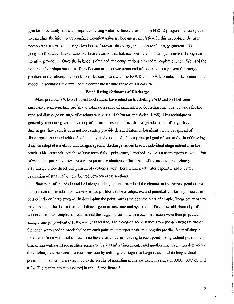
To illustrate this, figure 9 shows two schematic, idealized stratigraphic columns that correspond to the
flood records from CV and TC. This depiction assumes ideal conditions of deposition and preservation and
is purely for illustrative purposes. Nonetheless, it reveals the level of complexity that may be encountered
in attempting to unravel the historical record of flooding on the lower Verde River as recorded in the flood
stratigraphy, particularly for events less than about 2800 m3 S-1. This illustration underscores the potential
difficulties in correlating floods from various, disparate paleoflood sites on a river without the aid of a
reasonably detailed historical record and an adequate understanding of the flood hydrology of the basin.
Flood-Frequency Analysis
We used the results of our assessment of the potential underestimation of peak discharges based on
SWD to conduct a revised flood-frequency analysis of the Verde River. A previous analysis by Stedinger
and others (1986) using the MAX program incorporated paleoflood, historical, and systematic discharge
estimates for the Verde River. The MAX program uses maximum likelihood estimators in the statistical
analysis of both the systematic (gaged) and categorical (paleoflood) data. Categorical data is defined by the
number of occurrences or non-occurrences above specific magnitude thresholds over specified amounts of
time and is compatible with the nature of the paleoflood data. This statistical approach has proven to be
superior in extracting information from compound data sets as compared to the weighted moments
technique recommended by the United States Water Resources Council Bulletin 17b (1982) (Stedinger and
Baker, 1987; Lane, 1987, Condie and Lee, 1982). The statistical details of this approach and its
application to paleoflood data are provided by Stedinger and Cohn (1986), and Stedinger and others
(1986). In their original analysis, the use of paleoflood data produced a somewhat lower 100-year
discharge estimate than the historical and gage data only. In our revised analysis, we updated the
18
4000
A) (amp Verde
1993b
3000 . 1938
~ Q)
S -5 .sa = 19930 -"" c
Q) 0....
2000 - 1978b 1995b
19950
19800
19780 1980b
1970 I
1000 1937 -----j----1 1972
rJ 1951
B) Tangle Creek
4000 1891
19930
--_.? _.--
Pre·1891 1993b
3000
~ 19~00 19950
1938 Q)
S ..c: .!Z! =
1905 1978h 1920
19780 1995b
-"" c Q)
0.... 1951
2000
1916 1927 1972 1980b
1937 1970
1932 1966
1941 1000
Figure 9. Hypothetical flood-deposit stratigraphy from historical floods at sites near the Camp Verde and Tangle Creek gages on the Verde River. These stratigraphic sequences assume that deposits from all floods with peak discharges of greater than 1000 cms are preserved, and deposition occured up to the peak water surface. Deposits from smaller floods are inset into existing deposits, whereas larger floods overtop existing deposits. Discharges are listed in table 5.

systematic record through 1995, adjusted the paleoflood discharges upwards, and shortened the inferred
length ofthe geologic record of flooding.
In a previous paleoflood study on the Verde River, generalizations about the potential longevity of
flood scars and scour marks on canyon walls were used to extend the length of the paleoflood record to
2000 years (Ely and Baker, 1985). The geological arguments for these inferred record length are reasonable
but not very quantitative or well-constrained. In this analysis, we constrain the length of the flood record to
the estimated age of the oldest dated flood deposit on the lower Verde River (1000 BP). Also, because of
the influence of contributing area on the flood magnitudes along the Verde River, we concluded that
paleoflood data from the Red Creek reach cannot be reliably integrated with the gage data from TC.
Furthermore, our observations of the different amount of SWD-based underestimation at each site indicate
that use of a 5% factor in adjusting discharges from the Ely reach is appropriate.
In the flood-frequency analysis, we modeled two scenarios: (1) simply updating the original analysis
from Stedinger and others (1986) through 1995 to reflect the measurement oflarge floods at the gage in
1993 and 1995 (peaks of 4106 and 3058 m3 S-I, respectively), but making no other changes; (2) including
the updated historical record, shortening the total record length to coincide with the oldest dated paleoflood
event (1000 years), adjusting the SWD-based discharge estimates from the Ely reach by 5% and treating
the 1000 BP discharge estimate as a minimum constraint with no upper bound. We prefer scenario 2
because it incorporates more well-constrained paleoflood information and is probably a more realistic
treatment ofthe data.
The predicted 100-year flood from scenario 1 is essentially the same as the value reported by Stedinger
and others (1986) in the original analysis (table 7). This is somewhat surprising considering the addition of
two large floods, one of which (1993) is the flood of record. In scenario 2, the predicted 100-year flood
increased by 28% relative to the scenario 1 prediction .. Clearly, the addition of the two recent peaks
combined with the modifications of the paleoflood data have a significant effect on the results. Our revised
100-year flood estimate is comparable to estimates from various conventional statistical analyses of the
systematic and historical data (table 7); however, no statistical analysis of the historical and systematic
data listed in the table includes the most recent large floods.
Estimates of the magnitude of lower frequency events from our analysis as well as a variety of other
methods listed in table 7 stand in stark contrast to estimates of the probable maximum flood (PMF) on the
Verde River attributed to the U.S. Army Corps of Engineers and the U.S. Bureau of Reclamation (reported
in Ely and others, 1988). There is no geological evidence of such extreme flooding on the Verde River, and
we believe that it is reasonable to conclude that no floods approaching the reported PMF magnitudes have
19

Maximum Discharges
Paleoflood Studies (as reported)
Ely and Baker (1985) 5,400 O'Connor et al. (1986) 2,400 This study 1 5,474
Discharge-Drainage Area Relations
Malvick (1980) 5,950 Enzel et al. (1993) 2 6,500
Probable Maximum Flood
U. S. Army Corps of Engineers 3 18,970 U. S. Bureau of Reclamation 3 21,640
Statistical Analysis
Systematic and historical data 100-yr 500-yr 1000-yr
Anderson and White (1979) 4,500 Roeske (1978) 4,000 6,550 Gaffett and Gellenbeck(1989) 4,640
Geological, historical, and systematic data
Stedinger et a/. original 3,115 4,220 updated (scenario 1, this study) 3,144 4,083 4,475
This study (scenario 2) 4,021 5,350 5,936
notes
1. from section 7 rating curve
2. visual estimate from envelope curve
3. as reported in Ely et al. 1988
Table 7. Comparison of various theoretical and empirical estimates of discharge for the lower Verde River.

occurred on the Verde River during at least the last 10,000 years (i.e. the Holocene). If such extraordinary
floods had occurred in this time we would expect to find at least some compelling geomorphic evidence
attesting to that fact.
Conclusions
Our analysis of the 1993 floods on the Verde River illustrate that important advancements in
understanding the flood hydrology of a given drainage basin can result from integrating paleoflood data
with available gage and historical flood data. Our study also illustrates the potential magnitude of some
important uncertainties faced in most paleoflood reconstruction attempts. We found reasonably consistent
relationships between the elevations of slackwater deposits and ephemeral indicators of the actual peak
flood stage. In steep-walled depositional settings on the Verde River, slackwater deposits were about 1 m
below the peak water surface. Using these elevation differences in step-backwater modeling, we estimate
that discharge estimates based on slackwater deposits are about 30% less than the actual peak discharge. In
settings where confining slopes are more gentle, differences in these discharge estimates are less than 10%.
Using these relationships, we revised upward previously reported paleoflood estimates for the Verde River.
Corrections for discharge underestimation from reliance on SWD, recognition of the potentially great
importance of differences in contributing drainage area, and identification of undocumented SWD
stratigraphy contribute to a consistent relationship between discharges estimated at the two paleoflood
reaches and the upstream and downstream gages. This study conclusively demonstrates the importance of
understanding the flood hydrology of a river basin when interpreting paleoflood evidence in the basin.
Incorporation of our study results into previous paleoflood-based flood frequency analyses result in
higher predicted magnitudes for low-frequency events than previously reported. The new estimate ofthe so
called 100-year flood is comparable to that most recently reported by the USGS (Garrett and Gellenbeck,
1991); however, their analysis does not include the 1993 or 1995 floods. All of the statistical and empirical
predictions of low-frequency flood magnitudes listed in table 7 support the conclusion that assessments of
the PMF for the Verde River Basin is unrealistically large. Our field studies confirm that there is no
evidence of floods having such high magnitudes in the Holocene record of flooding.
Integrating our 1993 and revised paleoflood estimates with t.lJ.e gage data for the Verde River reveals
much about the complexity of flooding on this river system. The two large floods of 1993 behaved quite
differently and thereby increased our ability to understand the genesis oflarge floods on the Verde River.
This information can be related to gaged, historical, and paleoflood records alike. Many large floods of the
gaged record, including the February 1993 flood, emanated almost entirely from the upper Verde basin
above Cv. In the January 1993 flood, more than 65% of the peak discharge came from the lower 25% of
20

the Verde basin. This situation caused a rapid, dramatic increase in the peak discharge downstream of Cv.
As a consequence, sites only a few kilometers distant from one another along the lower Verde had
substantially different peak discharges. Similar but less extreme scenarios are evident in the systematic
record and very likely in the paleoflood record, a point with important implications for differences in
paleoflood stratigraphy at different sites along the river. The combined hydroclimatological and
hydrological characteristics that distinguished the floods of January and February 1993 establish a general
framework that easily substantiates the stratigraphic evidence for the occurrence of floods considerably
larger than the 1993 events.
References
Aldridge, B.N., and Eychaner, J.H., 1984, Floods of October 1977 in southern Arizona and March 1978 in central Arizona: US. Geological Survey Water-Supply Paper 2223, 143 pp.
Aldridge, B.N., and Hales, T.A., 1984, Floods of November 1978 to March 1979 in Arizona and westcentral New Mexico: US. Geological Survey Water-Supply Paper 2241, 149 pp.
Anderson, T.W., and White, N.D., 1979, Statistical summaries of Arizona streamflow data: US. Geological Survey Water-Resources Investigation 79-5,416 pp.
Baker, V.R, 1989, Magnitude and frequency ofpaeleofloods: in Floods: Hydrological, Sedimentological, and Geomorphologicallmplications, edited by K. Beven, and P. Carling, John Wiley, New York, pp. 171-183.
Baker, V.R, 1987, Paleoflood hydrology and extraordinary flood events: Journal of Hydrology, v. 96, p. 79-99.
Baker, V.R, and Kochel, RC., 1988, Flood sedimentation in bedrock fluvial systems: in Baker, V.R, Kochel, R C., and Patton, P. C., Flood Geomorphology: New York, Wiley, pp. 123-13 8.
Benson, M.A., and Dalrymple, T., 1967, General field and office procedures for indirect discharge measurements: USGS Techniques of Water Resource Investigations, Book 3, chapter A-I, 30 pp.
Chin, E.H., Aldridge, B.N., and Longfield, RJ., 1991, Floods of February 1980 in southern California and central Arizona: US. Geological Survey Professional Paper 1494, 126 pp.
Condie, R and Lee, K., 1982, Flood frequency analysis with historic information: Journal of Hydrology, vol. 58, pp. 47-61.
Dalrymple, T., and M.A. Benson, 1967, Measurement of peak discharge by the slope-area method: US. Geol. Surv. Techniques of Water Resource Investigations, Book 3, chapter A-2, 12 pp.
Ely, L.L., 1985, Reconstructing paleoflood hydrology with slackwater deposits: Verde River, Arizona: M.S. Thesis, Univ. Ariz., Dept. of Geosciences, 48 pp.
Ely, L.L., and Baker, V.R, 1985, Reconstructing paleoflood hydrology with slackwater deposits: Verde River, Arizona, Physical Geography, v. 6, pp. 103-126.
Ely, L.L., Y. Enzel, V.R Baker, and D.R Cayan, 1993, A 5000-year record of extreme floods and climate change in the southwestern United States: Science, n. 262, pp. 410-412.
21

Ely, L.L., O'Connor, J.E., and Baker, Y.R, 1988, Paleoflood hydrology of the Salt and Verde rivers, Central Arizona: in US. Committee on Large Dams, 8th Annual Lecture Series, Phoenix, Arizona, pp. 3.1 - 3.35
Enzel, Y, Ely, L.L, House, P.K, Baker, Y.R, and Webb, RH., 1993, Paleoflood evidence for a natural upper bound to flood magnitudes in the Colorado River Basin: Water Resources Research, v. 29, no. 7, pp. 2287-2297.
Garrett, J.M., and D.J. Gellenbeck, 1991, Basin characteristics and streamflow statistics in Arizona as of 1989: US.Geol. Surv Water Resour. Invest., 91-4041, 612 pp.
Hoggan, D.H., 1989, Computer-assisted floodplain hydrology and hydraulics, McGraw-Hill, New York, 518 pp.
House and Pearthree, in press, A geomorphologic and hydrologic evaluation of an extraordinary flood discharge estimate: Bronco Creek, Arizona: Water Resources Research.
House, P.K, and KK Hirschboeck, 1995, Hydroclimatological and paleohydrological context of extreme winter flooding in Arizona, 1993: Arizona Geological Survey Open-File Report 95-12, 44 pp.
Hydrologic Engineering Center, 1985, HEC-2 water surface profiles users manual, US. Army Corps of Eng., Davis, Calif., 37 pp.
Kochel, RC., 1988, Extending stream records with slackwater paleohydrology: examples from west Texas, in Flood Geomorphology, edited by Y.R Baker, R.C. Kochel, and P .C. Patton, John Wiley, New York, pp. 377-392.
Kochel, RC., and Y.R. Baker, 1988, Paleoflood analysis using slackwater deposits, in Flood Geomorphology, edited by Y.R Baker, RC. Kochel, and P.C. Patton" John Wiley, New York, pp. 357-376.
Lane, W.L., 1987, Paleohydrologic data and flood frequency estimation, in Singh, Y.P. ed. Regional Flood Frequency Analysis: D. Reidel Publishers, Boston, pp. 287-298.
Malvick, A.J., 1980, A magnitude-frequency-area relation for floods in Arizona:. A study to advance the methodology of assessing the vulnerability of bridges to floods for the Arizona Department of Transportation: The Engineering Experiment Station, Gen. Rpt. No.2, Univ .. Ariz. Tucson, 185 pp.
O'Connor, J.E., and R H. Webb, 1988, Hydraulic modeling for paleoflood analysis, in Flood Geomorphology, edited by Y.R Baker, RC. Kochel, and P.C. Patton, John Wiley, New York, pp. 393-402.
O'Connor, J.E., Fuller, J.E., and Baker, Y.R, 1986, Late Holocene flooding within the Salt River basin, central Arizona: Unpublished report to the Salt River Project, 84 pp.
O'Connor, J.E., L.L. Ely, E.E. Wohl, L.E. Stevens, T.E. Melis, Y.S. Kale, and Y.R Baker, 1994, A 4500-year record oflarge floods on the Colorado River in the Grand Canyon, Arizona, J Geol., n. 102, pp. 1-9.
Patterson, J.L., and Somers, W.P., 1966, Magnitude and frequency of floods in the United States: Part 9. Colorado River Basin: US. Geological Survey Water-Supply Paper 1683, 476 pp.
Roeske, RH., 1978, Methods for estimating the magnitude and frequency of floods in Arizona: Arizona Dept. of Transportation Research Project HPR -1-15 (121), 82 pp.
Stedinger, J.R and Baker, Y.R, 1987, Surface water hydrology: historical and paleoflood information: Reviews of Geophysics, v. 25, pp. 199-124.
22
Stedinger, J.R, and Cohn, T.A., 1986, Flood frequency analysis with historical and paleoflood infonnation: Water Resources Research, v. 22, pp. 785-793.
Stedinger, J., Therivel, R, Grygier, J., Wu, RS, 1986, Analysis of the frequency of large floods on the Salt and Verde rivers using historical and paleoflood infonnation: Unpublished repOlt to the Salt River Project, Phoenix, Arizona.
United States Water Resources Council, 1982, Guidelines for detennining flood flow frequency, Bulletin 17b of the Hydrology Committee: United States Water Resources Council, Washington, D.C.
23


