Hybrid-Degree Weighted T-splines and Their
Application in Isogeometric Analysis
Lei Liua, Hugo Casquerob, Hector Gomezb, Yongjie Jessica Zhanga,∗
aDepartment of Mechanical Engineering, Carnegie Mellon University, Pittsburgh, PA15213, USA
bDepartamento de Metodos Matematicos, Universidade da Coruna, Campus de ACoruna, 15071, A Coruna, Spain
Abstract
In this paper, we introduce hybrid-degree weighted T-splines by means of lo-
cal p-refinement and apply them to isogeometric analysis. Standard T-splines
enable local h-refinement, however, they do not support local p-refinement.
To increase the flexibility of T-splines so that local p-refinement is also avail-
able, we first define weighted B-spline curves of hybrid degree. Then we
extend the idea to weighted T-spline surfaces of hybrid degree. A transition
region is defined so as to stitch the locally p-refined region with the rest of
the mesh. The transition region has the same basis function degree as the
p-refined region, and the same surface continuity as the rest of the mesh.
Finally, we compare the performance of odd-, even-, and hybrid-degree T-
splines over an L-shaped domain governed by the Laplace equation and create
high-genus surfaces using hybrid-degree weighted T-splines.
Keywords: Arbitrary Degree, Analysis-suitable T-splines, Weighted
T-splines, Hybrid Degree, Local p-refinement, Isogeometric Analysis
∗Corresponding author: Yongjie Jessica Zhang, Tel: (412) 268-5332; Fax: (412) 268-3348; Email: [email protected].
Preprint submitted to Computers & Fluids September 28, 2015

1. Introduction
Isogeometric analysis (IGA) adopts the same basis functions for geomet-
ric modeling and numerical analysis in order to fill the gap between these
two fields [1]. Currently, the two popular basis functions in IGA are non-
uniform rational B-splines (NURBS) [2–4] and T-splines [5–7]. The higher
interelement continuity of these spline spaces leads to significant advantages
in analysis in comparison with C0-continuous Lagrange polynomials used in
the conventional finite element method such as, e.g., enhanced robustness
in structural mechanics [8], improved accuracy per degree-of-freedom in fluid
mechanics [9], among others. Fluid-structure interaction (FSI) methods ben-
efit from the aforementioned advantages and have been an active field in IGA,
both body-fitted methods [10–15] and immersed methods [16–20] have been
investigated. Furthermore, the higher continuity of splines enables to solve
higher-order partial differential equations in primal form [21–27] and to col-
locate partial differential equations in strong form [7, 28–32].
The efficiency of any computational method depends strongly on its local
refinement capabilities. Unfortunately, NURBS only allow global refinement,
which is an important limitation in both design and analysis. T-splines
were presented as a generalization of NURBS that allow local h-refinement
by introducing T-junctions. T-splines were presented in CAD in [5] and
brought to analysis in [6]. An important subset of T-splines was later defined,
the so-called analysis-suitable T-splines (ASTS). ASTS were mathematically
shown to satisfy all the important mathematical properties of NURBS while
maintaining the local h-refinement capability of T-splines. This was first
2

demonstrated for cubic ASTS [33–36] and then for arbitrary degrees [37, 38].
The subset of ASTS is defined based on a simple topological constraint,
namely, T-junction extensions from different parametric directions cannot
meet with each other. T-splines with arbitrary topology can be obtained by
introducing extraordinary nodes. The topological constraints in order to get
cubic ASTS in the presence of extraordinary nodes were explained in [39].
Finally, these topological constraints can be relaxed by the use of weighted
T-splines leading to higher flexibility [40, 41].
Local h-refinement of T-splines was first studied in [42], introducing the
refinement matrix. An optimized T-junction extension algorithm was devel-
oped for local h-refinement of analysis-suitable T-splines [43]. Some adaptive
h-refinement schemes have a linear computational complexity [44, 45], pre-
serving linear independence of the basis functions. Hierarchical T-splines
were proposed in [46], together with its analysis-suitability and refinabil-
ity. Truncated hierarchical basis functions were also used to perform local
h-refinement while ensuring partition of unity and linear independence, such
as truncated hierarchical B-splines (THB) [47] and truncated hierarchical
Catmull-Clark surfaces (THCCs) [48, 49].
As local h-refinement of T-splines was well studied, local p-refinement
of T-splines has not been studied yet. Basis functions with elevated degree
need to be defined over the whole geometry for global p-refinement. Degree
elevation of B-spline curves was first studied in [50], which presents an algo-
rithm to elevate the degree by one. Efficient algorithms were developed to
raise the degree of B-spline curves/surfaces by representing a curve/surface
of degree m with the linear combination of curves/surfaces of degree m + 1
3

[51, 52]. Then a fast algorithm was developed to elevate the degree by arbi-
trary times [53]. A software-engineering approach was presented for degree
elevation of B-spline curves with competitive performance in speed and ac-
curacy [54]. Bezier basis functions were also used for the degree elevation
of B-splines, which first raise the degree of Bezier elements and then remove
unnecessary knots for desired surface continuity [2]. Multi-degree splines
were first introduced comprising segments with different degrees of at most
3 in one spline curve [55], where the basis functions are defined based on
knot intervals like regular B-splines. Then the basis was extended with ar-
bitrary various degrees and improved curve continuity [56]. A de Boor-like
evaluation approach for multi-degree spline curves was then developed which
supports local h-refinement by knot insertion and Bezier representation [57].
However, spline surfaces of multiple degree have not been studied yet.
In this work, we study weighted T-spline basis functions of both odd and
even degree in detail. With a designed T-mesh splitting scheme, hybrid-
degree weighted T-splines are proposed, supporting both local p-refinement
and local h-refinement. The local p-refinement introduces a limited number
of new control points to the T-mesh. Basis functions of different degrees are
defined over the domain. The degree of basis functions of the refined re-
gion and transition region is elevated by one after local p-refinement. An L-
shaped domain is parameterized with odd-, even- and hybrid-degree weighted
T-splines. The Laplace equation is solved over this domain, showing the ad-
vantage of hybrid-degree T-splines. High-genus surfaces with extraordinary
nodes are also parameterized with hybrid-degree weighted T-splines.
The layout of this paper is as follows. T-splines of arbitrary degree are re-
4

viewed in Section 2, together with arbitrary-degree weighted T-splines. How
to generate hybrid-degree weighted T-splines is given in Section 3. Isogeo-
metric analysis is performed over over hybrid-degree weighted T-splines in
Section 4 and various high-genus surfaces are constructed. The conclusions
are given in Section 5 with proposed future work.
2. Arbitrary Degree T-splines
T-splines of arbitrary degree are briefly reviewed here. For further details,
we suggest the readers refer to [5–7, 42]. T-splines discussed here have the
same degree in the two parametric directions. We classify them into even- and
odd-degree T-splines. T-splines with p = 2 and p = 3 are used as examples to
explain the definitions and show the comparison. T-splines of higher degree
can be deduced analogously.
2.1. T-spline Basics
A T-mesh contains all the topological information of a T-spline and is
composed of vertices, edges and faces. Knot intervals are non-negative real
numbers assigned to T-mesh edges. A valid T-mesh configuration requires
that the sum of knot intervals assigned to opposite edges of a face stays the
same. To maintain the open knot vector property, T-meshes have ⌊p/2⌋ rings
of edges with zero-length knot intervals, where the ⌊⋅⌋ represents the integer
part of a real number. For example, Fig. 1(a) shows a T-mesh with one ring
of edges with zero-length knot intervals. The unshaded faces have edges with
zero-length intervals. This T-mesh can be used to define basis functions of
either p = 2 or p = 3.
5

(a) (b) (c) (d) (e)
Figure 1: (a) T-mesh with two selected T-junctions marked with blue squares. The T-
meshes with extensions of these two T-junctions are given in (b) when p = 2 and (c) when
p = 3. The solid red lines represent edge extensions, and the dashed red lines represent
face extensions. (d) and (e) show the elemental T-mesh when p = 2 and p = 3, respectively.
T-junctions are the interior vertices of valance-3 and analogous to hang-
ing nodes in finite element meshes. The blue squares in Fig. 1(a) are two
selected T-junctions. T-junction extension was first discussed in [36], includ-
ing face extension and edge extension. A face extension is a line obtained by
moving from the T-junction along the missing edge direction until ⌊(p+1)/2⌋orthogonal edges are encountered. An edge extension is a line obtained by
moving opposite to the face extension direction until ⌊p/2⌋ orthogonal edges
are encountered. For example in Fig. 1(b, c), the face extensions are marked
with dashed red lines, and edge extensions are marked with solid red lines
when p = 2 and p = 3. For general analysis-suitable T-splines of arbitrary de-
gree, it is required that T-junction extensions cannot meet with each other
from different parametric directions [37]. Edge and face extensions are used
to check if analysis-suitable requirements are satisfied by the T-mesh. By
only drawing all the face extensions and excluding faces with zero-length in-
terval edges in the T-mesh, we obtain the elemental T-meshes as shown in
Fig. 1(d, e).
6
(a) (b)
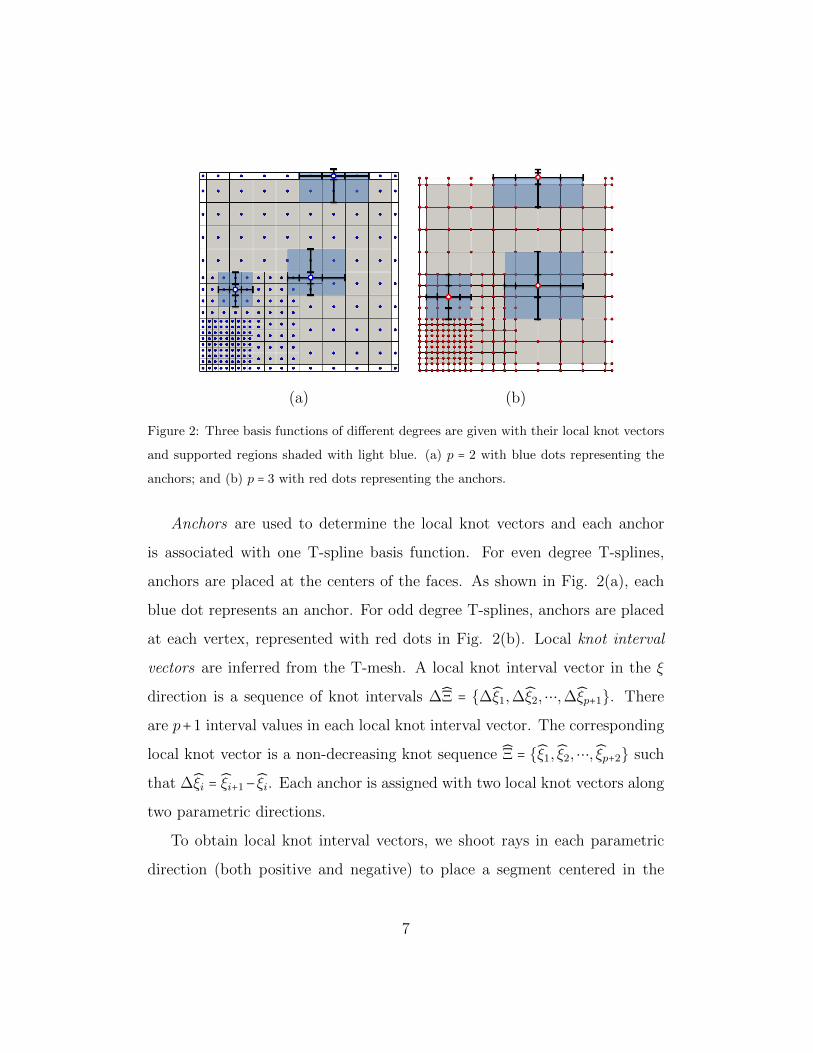
Figure 2: Three basis functions of different degrees are given with their local knot vectors
and supported regions shaded with light blue. (a) p = 2 with blue dots representing the
anchors; and (b) p = 3 with red dots representing the anchors.
Anchors are used to determine the local knot vectors and each anchor
is associated with one T-spline basis function. For even degree T-splines,
anchors are placed at the centers of the faces. As shown in Fig. 2(a), each
blue dot represents an anchor. For odd degree T-splines, anchors are placed
at each vertex, represented with red dots in Fig. 2(b). Local knot interval
vectors are inferred from the T-mesh. A local knot interval vector in the ξ
direction is a sequence of knot intervals ∆Ξ = ∆ξ1,∆ξ2,⋯,∆ξp+1. There
are p+1 interval values in each local knot interval vector. The corresponding
local knot vector is a non-decreasing knot sequence Ξ = ξ1, ξ2,⋯, ξp+2 such
that ∆ξi = ξi+1− ξi. Each anchor is assigned with two local knot vectors along
two parametric directions.
To obtain local knot interval vectors, we shoot rays in each parametric
direction (both positive and negative) to place a segment centered in the
7

anchor crossing exactly p + 2 orthogonal edges. Note that “centered in the
anchor” means that the segment crosses the same number of orthogonal edges
on the left- and right-hand sides of the anchor, and spans a particular set of
p + 1 edges. The knot interval values of the spanned edges are placed into
the local knot interval vector consecutively. Zero-length edges are appended
when a boundary is crossed before enough orthogonal edges are found.
Based on the local knot interval vectors, local knot vectors are obtained
and T-spline basis functions are defined. If a T-spline basis function has non-
zero value over one region covered in the T-mesh, then it has support over
the geometry in the physical domain extracted from that region. The light
blue regions in Fig. 2 show the support of different T-spline basis functions
associated with the selected anchors.
T-splines of arbitrary degree are defined element-wise. For element e
in the elemental T-mesh, suppose Ne = N ei (ξ, η)n
e
i=1 is the vector of T-
spline basis functions having support over e. N ei (ξ, η) is the basis function
mapped to the parent element ◻ = [−1,1]2 with the affine map introduced in
[58]. Then the T-spline geometry is defined by the element geometric map,
xe ∶ ◻→ Ωe, from the parent element domain to the physical domain as
xe =
ne
∑i=1wiPe
iNei (ξ, η)
ne
∑i=1wiN e
i (ξ, η), (1)
where Pei is the corresponding control point of the basis function N e
i (ξ, η),and wei is the corresponding weight. Note that Pe
i , wei are all mapped from
global to local numbering by the IEN array [58] such that Pei = PIEN(i,e) and
wei = wIEN(i,e). The element control points Pe is a matrix of dimension ne×ds,
8

where ds is the spatial dimension. Analysis-suitable T-splines of arbitrary
degree satisfy polynomial partition of unity, which meansne
∑i=1N ei (ξ, η) = 1.
When wei = 1.0 for any Pei , Eqn. (1) is simplified as
xe =ne
∑i=1
PeiN
ei (ξ, η). (2)
In the following, we set the weights of all the control points are 1.0 for the
sake of brevity.
2.2. Bezier Element Extraction
Based on the Bezier extraction algorithm [58, 59], T-spline basis functions
can be represented as linear combinations of Bezier basis functions. Each
element in the elemental T-mesh corresponds to one Bezier element. The eth
Bezier element in the physical domain can be represented as
xe =ne
∑i=1
PeiN
ei (ξ, η) =
ne
∑i=1
Pei
(p+1)2∑j=1
M eijBj(ξ, η), (3)
where Bj(ξ, η) is the jth Bezier basis function defined on the parent element,
and M eij is the Bezier extraction coefficient. By converting Eqn. (3) to matrix
format, we have
xe = (Pe)TNe = (Pe)TMeB, (4)
(a) (b)
Figure 3: Locally h-refined T-splines with Bezier representation. (a) p = 2; and (b) p = 3.
9

where Pe is the matrix of control points, Me is the Bezier extraction matrix,
and B is the vector of Bezier basis functions. Eqn. (4) is the Bezier element
representation of T-splines. Fig. 3 shows a rectangular domain parameterized
with locally h-refined T-splines and Bezier element representations when p = 2
and p = 3.
2.3. Arbitrary-Degree Weighted T-splines
The subset of ASTS is defined based on a simple topological constraint,
namely, horizontal T-junction extensions cannot meet with vertical T-junction
extensions. If the quadtree subdivision algorithm is applied to a T-mesh, the
resulting T-mesh may violate the topological constraint mentioned above and
polynomial partition of unity may not be satisfied. However, polynomial par-
tition of unity can be recovered through the use of weighted T-splines [40].
Weighted T-splines enable to use more simple and localized h-refinement
strategies over the T-mesh such as, e.g., quadtree subdivision. For a T-
spline basis function Nj(ξ, η) with corresponding control point Pj obtained
from the knot insertion algorithm, if partition of unity is satisfied in all
the support of Nj(ξ, η), then the weighted T-spline basis function Nj(ξ, η)equals to Nj(ξ, η) and Pj equals to Pj. Otherwise for Nj(ξ, η), the weighting
coefficients of children basis functions [40] or extracted Bezier basis functions
[41] are modified to obtain Nj(ξ, η). The control points associated with
modified basis functions are computed solving a linear system [40]. The
detailed weighting coefficient modification algorithm is explained as follows.
Given a T-mesh, the weighted T-spline of degree p on the eth Bezier
element is defined as
10
xe =ne
∑j=1
PejN
ej (ξ, η) =
ne
∑j=1
Pej
(p+1)2∑k=1
M ejkBk(ξ, η) = (Pe)TMeB, (5)
where N e(ξ, η) are the weighted T-spline basis functions with support over
this Bezier element, Pej are the corresponding control points. Me is the ma-
trix which transfers weighted T-spline basis functions to Bezier basis func-
tions. Bk(ξ, η) is the Bezier basis function. The IEN array is also used here
to handle the mapping from global to local numbering.
To obtain Me, we first calculate the Bezier transformation matrix Me for
regular T-spline basis functions N ej (ξ, η). Note that with Me, partition of
unity may not be satisfied everywhere. For a Bezier basis function Bk(ξ, η),the summation of calculated weighting coefficients (
ne
∑j=1M e
jk) from N ej (ξ, η)
may not be 1.0. We modify Me to Me such that
M ejk =
M ejk
ne
∑i=1M e
ik
. (6)
Consequently, the regular T-spline basis functions are replaced with weighted
T-spline basis functions and
ne
∑j=1M e
jk = 1, k = 1,2,⋯, (p + 1)2 (7)
is always satisfied. Since Bezier basis functions satisfy partition of unity, we
havene
∑j=1N ej (ξ, η) =
ne
∑j=1
(p+1)2∑k=1
M ejkBk(ξ, η) = 1, (8)
and weighted T-splines always satisfy polynomial partition of unity.
Note that we are normalizing each column of Me to obtain Me according
to Eqn. (6). This modification only involves elementary matrix operation
11

and does not change the rank of the matrix. Since Me is in full-rank, Me is
also in full-rank. So the weighted T-splines of arbitrary degree are linearly
independent [36, 40, 41].
3. Hybrid-Degree Weighted T-splines
In this section, we introduce our algorithm to construct hybrid-degree
weighted T-splines by means of local p-refinement. We first introduce hybrid-
degree B-spline curves, and then generalize the ideas to hybrid-degree weighted
T-spline surfaces.
3.1. Hybrid-Degree B-spline Curves
Generally for B-splines, global degree elevation increases the degree of all
the basis functions. Suppose a cubic B-spline is defined on the open knot vec-
tor U = u0, u0, u0, u0, u1, u2, ..., un, un, un, un. There are n+3 basis functions.
To elevate it to quartic, each unique knot value in U is duplicated once to form
the new open knot vector U = u0, u0, u0, u0, u0, u1, u1, u2, u2, ..., un, un, un, un, un,
based on which 2n + 3 new quartic B-spline basis functions are defined. The
detailed algorithm can be found in [2]. B-spline global degree elevation can
increase the degree of basis functions without modifying the geometry [2].
The disadvantages are that a lot of new control points are calculated and the
interelement continuity is not increased.
To construct hybrid-degree B-spline curves by means of local p-refinement,
we define the spline basis functions on local knot vectors instead of using a
global knot vector, which is analogous to what is done in T-splines. Fig. 4(a)
shows part of a cubic B-spline curve in the index space, where the orange
edge has knot interval value 0 and the black edges have knot interval value 1.
12

(a) (b)
(c) (d)
(e) (f)
Figure 4: Local p-refinement of B-splines of p = 3. (a) The mesh of B-spline in the
index space, where the orange edge has knot interval value 0, and the black edges have
knot interval value 1; (b) the mesh in the parametric space, where the green edge is set
as the hybrid boundary; (c) the red squares represent the anchors to define cubic basis
functions; (d) for the green edge, the corresponding anchors to define supporting cubic
and quartic basis functions of are represented with the crossed-out red squares and blue
circles, respectively; (e) quartic basis functions are defined on the p-refined region; and (f)
the resulting anchors to define cubic and quartic basis functions . Both cubic and quartic
basis functions have support over the magenta transition region.
The B-spline in the parametric space is given in Fig. 4(b) with parametric
values. The red squares in Fig. 4(c) represent the anchors to define cubic
basis functions before p-refinement. To perform local p-refinement, we define
basis functions of degree p + 1 only on the refined region.
Knot Insertion. A Hybrid boundary is the edge where we add knots to
its ends so as to stitch the p-refined region with the rest of the curve. In Fig.
4(b), suppose we want to perform local p-refinement to the region u ≤ 4, then
the edge marked in green is the hybrid boundary.
There are four cubic basis functions (N3i (u),4 ≤ i ≤ 7) that have support
13

over the green edge before p-refinement. They are defined on local knot vec-
tors 0,1,2,3,4, 1,2,3,4,5, 2,3,4,5,6, 3,4,5,6,7, respectively. The
corresponding anchors are represented with crossed-out red squares in Fig.
4(d). To perform local p-refinement, two new knots (3 and 4) are inserted.
There are five quartic basis functions (N4i (u),5 ≤ i ≤ 9) with support over
the green edge (see Fig. 5(b)). They are defined on local knot vectors
0,1,2,3,3,4, 1,2,3,3,4,4, 2,3,3,4,4,5, 3,3,4,4,5,6, 3,4,4,5,6,7,
respectively, and the corresponding anchors are represented with blue circles
in Fig. 4(d). To preserve the open knot vector property, zero knot is also
inserted, shown in Fig. 4(e, f).
Definition of Basis Functions. We disactivate the basis functions of
degree p having support over the p-refined region and activate basis functions
of degree p+1 that have support over this region. In the p-refined region
(u ≤ 4), quartic basis functions are defined. The final anchors to define basis
functions over the whole domain are shown in Fig. 4(f). The defined basis
functions before and after local p-refinement as depicted in Fig. 4 are shown
in Fig. 5(a, b). In Fig. 5(a), the dashed red lines are the removed cubic
basis functions from the p-refined region. The solid blue lines in Fig. 5(b)
show the newly defined quartic basis functions in the p-refined region.
Transition Region. A Transition region connects the refined region
and the unchanged region. Only basis functions of degree p+ 1 have support
over the refined region (0 ≤ u ≤ 4 in Fig. 5(b)). Only basis functions of
degree p have support over the unchanged region (u ≥ 7 in Fig. 5(b)). Basis
functions of both degree p and p + 1 have support over the transition region
(4 ≤ u ≤ 7 in Fig. 5(b)). We use hybrid-degree B-splines to represent the
14
(a) (b)
4 5 4 5 4 5
(c) (d) (e)
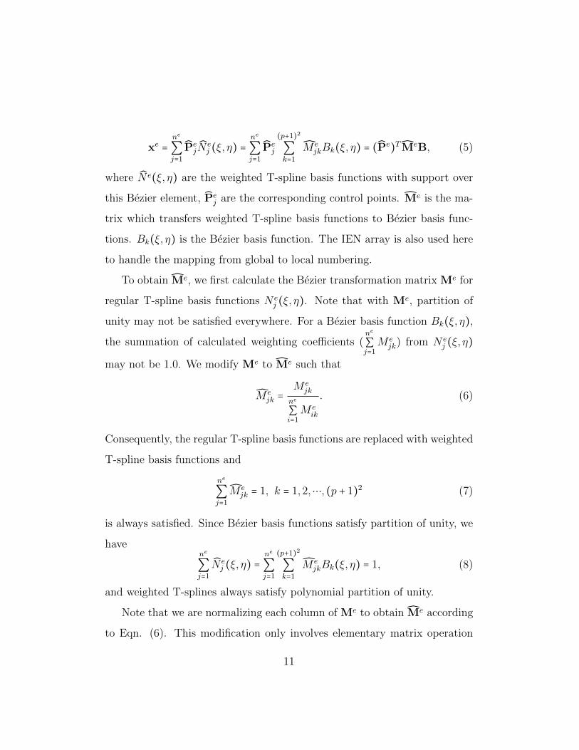
Figure 5: (a) Basis functions of p = 3 (red), where the dashed red basis functions are
removed; (b) basis functions of p = 4 (blue) are defined on the refined region; (c) Bezier
basis functions of p = 4 over region 4 ≤ u ≤ 5; (d) weighted Bezier basis functions obtained
from Eqn. (13); and (e) the difference between (c) and (d).
geometry over this region. Let us take the edge at 4 ≤ u ≤ 5 as an example.
There is one cubic basis function (N38 (u)) and three quartic basis functions
(N4i (u),7 ≤ i ≤ 9) having support over it, shown in Fig. 5(b). To define the
geometry, we have
x = P38N
35 (u) +
9
∑i=7
P4iN
4i (u), (9)
where P38, P4
i are the corresponding control points of the basis functions
N38 (u) and N4
i (u) respectively. P38 is the 8th vertex in the control polygon of
the original cubic B-spline. P4i are the center points of each control polygon
edge, which are obtained by linear interpolation of the two vertices of the
15

polygon edge. By representing the B-spline basis functions with Bezier basis
functions, we have
x = Pe,p8
4
∑j=1M e,p
8j Bpj (u) +
9
∑i=7
Pe,p+1i
5
∑k=1M e,p+1
ik Bp+1k (u)
=4
∑j=1
Qe,pj Bp
j (u) +5
∑k=1
Qe,p+1k Bp+1
k (u),(10)
where p = 3, M e,p8j and M e,p+1
ik are the Bezier extraction coefficients. Qe,pj and
Qe,p+1k are the Bezier control points. Based on the degree elevation algorithm
for Bezier elements [2], we have
Qe,p+1i = (1 − i − 1
p + 1)Qe,p
i + i − 1
p + 1Qe,pi−1, i = 1,2,⋯, p + 2. (11)
When i = 1, i−1p+1 = 0 and when i = p + 2, 1 − i−1
p+1 = 0. The undefined Qe,p0
and Qe,pp+2 do not jeopardize the integrity of Eqn. (11) and we set them as 0.
We move the superscript p of control points and Bezier extraction matrix to
subscript for convenience, and convert Eqn. (10) to matrix format
xe = (Pep)TMe
pBp + (Pe
p+1)TMep+1B
p+1 = (Qep)TBp + (Qe
p+1)TBp+1. (12)
With Eqn. (11), Eqn. (12) is converted to
xe = (Qep)TTp+1
p Bp+1 + (Qep+1)TBp+1 = (Pe
p)TMepT
p+1p Bp+1 + (Pe
p+1)TMep+1B
p+1
= ((Pep)TMe
pTp+1p + (Pe
p+1)TMep+1)Bp+1 = RTM
e
p+1Bp+1,
(13)
where Tp+1p is obtained from Eqn. (11), R are the control points. M
e
p+1 is
the transformation matrix, and Bp+1 represent Bezier basis functions.
Partition of unity is not satisfied here. We recover partition of unity
through the use of weighted T-splines as explained in Section 2.3. Fig. 5(c)
16
shows the five quartic Bezier basis functions. The calculated weights of the
five Bezier basis functions obtained from Me
p+1 are 1.0,1.0,0.95833,0.95833
and 1.0, respectively. The weighted Bezier basis functions are shown in Fig.
5(d). The differences are shown in Fig. 5(e). Finally Eqn. (13) is converted
to
xe = RTMep+1B
p+1, (14)
which is used to define the hybrid-degree weighted B-splines over the transi-
tion region.
Remark 3.1. The hybrid B-spline defined over the transition region
is of degree p + 1, since we performed degree elevation to the Bezier basis
functions of degree p. But the surface continuity is Cp−1, which is the same
as the unchanged region. The reason is that basis functions of degree p have
support over this region.
3.2. Local p-refinement of T-splines
To explain local p-refinement of T-splines, we define the graph connecting
all the faces to introduce new zero-length edges as the hybrid boundary.
There are two types of hybrid boundaries, namely the interior boundary and
the extended boundary. Interior boundaries are the loops within the domain.
Extended boundaries contain faces lying on the boundary of the geometry.
We constrain that the hybrid boundaries cannot be reached by face extension
of any T-junction. In this way, T-junctions do not influence the faces lying
on the hybrid boundaries.
There are mainly three steps to perform local p-refinement. We first
determine the local parametric directions to split the faces on the hybrid
17
boundaries. Then we split the faces along the detected directions to introduce
zero-length interval edges to the T-mesh. After the splitting we define higher
order basis functions over the p-refined region. The last step is to decide the
active original basis functions and calculate the new control points.
Here we take the T-mesh in Fig. 6(a) as an example. Since there is only
one ring of edges with zero-length intervals on the boundary of the T-mesh,
both basis functions of p = 3 and p = 2 can be defined on it. The three steps
are explained mainly based on odd degree T-splines. Even degree T-splines
are used to explain the difference and show the comparison.
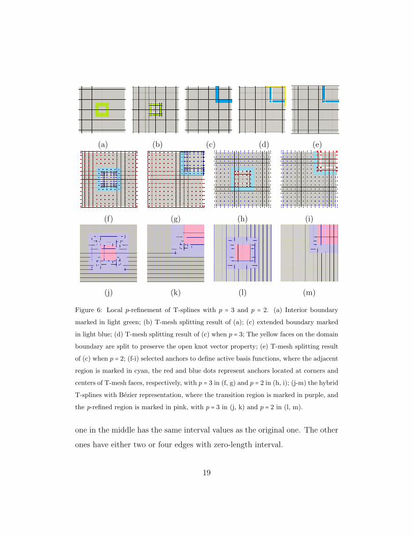
Local Splitting Direction Detection (Step 1). Fig. 6(a) and (c)
show the interior and extended hybrid boundaries of the T-mesh, marked
in light green and light blue, respectively. We split the faces on the hybrid
boundaries to introduce zero-length interval edges across them. For a pair
of neighboring faces sharing an edge on the hybrid boundary, the splitting
direction is perpendicular to that edge. If a face has edges of two differ-
ent directions shared by other faces on the hybrid boundary, it should be
split in both directions. For example the faces on the corners of the hybrid
boundaries in Fig. 6(a) and (c) should be split in both directions.
T-mesh Splitting and Basis Function Definition (Step 2). With
the detected splitting directions, we split the faces on the hybrid boundaries
as shown in Fig. 6(b). If one face should be split in one direction, we split it
into three new faces. The new face in the middle has the same edge interval
values as the original faces, see the light green faces. The other two have
zero-length interval across the splitting direction, see the unshaded faces. If
a face should be split in both directions, nine new faces are generated. The
18
(a) (b) (c) (d) (e)
(f) (g) (h) (i)
(j) (k) (l) (m)
Figure 6: Local p-refinement of T-splines with p = 3 and p = 2. (a) Interior boundary
marked in light green; (b) T-mesh splitting result of (a); (c) extended boundary marked
in light blue; (d) T-mesh splitting result of (c) when p = 3; The yellow faces on the domain
boundary are split to preserve the open knot vector property; (e) T-mesh splitting result
of (c) when p = 2; (f-i) selected anchors to define active basis functions, where the adjacent
region is marked in cyan, the red and blue dots represent anchors located at corners and
centers of T-mesh faces, respectively, with p = 3 in (f, g) and p = 2 in (h, i); (j-m) the hybrid
T-splines with Bezier representation, where the transition region is marked in purple, and
the p-refined region is marked in pink, with p = 3 in (j, k) and p = 2 in (l, m).
one in the middle has the same interval values as the original one. The other
ones have either two or four edges with zero-length interval.
19

In the p-refined region, if there are faces on the boundary of the domain,
then the open knot vector property should be satisfied after T-mesh splitting.
When performing local p-refinement to T-splines of odd degree, one new
boundary layer with zero-length interval edges is introduced. For T-mesh
in Fig. 6(c), if p = 3, there is one layer of faces with zero-length intervals.
After refining it to p = 4, there should be two layers. We equally split the
faces on the geometric boundary to two smaller ones. The splitting follows
the direction of the geometry boundary. If the face is at the corner of the
geometry, it is equally split into four smaller ones. In Fig. 6(d), those faces
marked in yellow are the newly generated faces with zero-length intervals. If p
is even, no boundary face splitting is required to satisfy the open knot vector
property. In Fig. 6(e), faces on the geometric boundary remain unchanged,
except those on the extended hybrid boundary.
After T-mesh splitting, we place anchors on both the corners and the
centers of T-mesh faces. Local knot vectors are inferred for each anchor. For
an anchor at the corner, a T-spline basis function of odd degree is defined.
Whereas for an anchor at the center, a T-spline basis function of even degree
is defined.
We define an adjacent region as the first-ring neighborhood of the hybrid
boundary beyond the p-refined region. In Fig. 6(f - i), the adjacent regions
are marked in cyan. All the basis functions of degree p + 1 in the p-refined
region are set as active. All basis functions of degree p beyond the adjacent
region are also set as active. When p is odd, the basis functions of degree
p + 1 at the face center in the adjacent region are set as active. In Fig. 6(f,
g), the anchors to define active cubic basis functions are represented with
20

red dots. The anchors to define active p-refined quartic basis functions are
represented with blue dots. When p is even, the basis functions of degree
p + 1 at the corners shared by the adjacent region and the hybrid boundary
are set as active. In Fig. 6(h, i), the anchors to define active quadratic basis
functions are represented with blue dots, and the anchors to define active
cubic basis functions are represented with red dots.
Control Point Calculation (Step 3). Local p-refinement may slightly
change the geometry. The refinement algorithms introduced in [2] to calculate
control points cannot be used here because zero-length interval edges are only
introduced along the hybrid boundary. Here we introduce a direct way to
calculate the new control points from the original ones by linear interpolation.
We place five control points on each T-mesh element. Four are at the
corners and the last one is in the center. If p is odd, we use corner points
to interpolate the center control points for the new basis functions of degree
p + 1. For example in Fig. 7(a), a center control point C1 is calculated by
C1 =P1 +P2 +P3 +P4
4, (15)
where P1 ∼ P4 are four control points at the corners. If p is even, we use
center points to perform the interpolation. In Fig. 7(b), a corner control
point P1 is calculated by
P1 =∆ξ2∆η2C1 +∆ξ1∆η2C2 +∆ξ1∆η1C3 +∆ξ2∆η1C4
(∆ξ1 +∆ξ2)(∆η1 +∆η2), (16)
where C1 ∼ C4 are four control points at the centers of the elements which
share P1. After the T-mesh splitting and control point calculation, we can
define the hybrid-degree weighted T-splines.
21

(a) (b)
Figure 7: Interpolation scheme to obtain new control points. (a) Using corner control
points to calculate the center control point; and (b) using center control points to calculate
the corner control point.
3.3. Hybrid-Degree Weighted T-spline Construction
We define the hybrid-degree weighted T-splines with Bezier element rep-
resentation. In the p-refined region, only basis functions of degree p+ 1 have
support over extracted Bezier elements. In the unchanged region, only ba-
sis functions of degree p have support over extracted Bezier elements. Both
basis functions of degree p and p+1 have support over the Bezier elements ex-
tracted from the transition region. There are ⌊(p+1)/2⌋+1 rings of elements
in the transition region (see Fig. 6(j-m)).
Bezier elements in the p-refined or unchanged region are calculated using
Eqn. (4). Over the transition region, the hybrid-degree T-spline for the eth
element is defined as
xe =∑m
PemN
e,pm (ξ, η) +∑
n
CenN
e,p+1n (ξ, η) (17)
22
when p is odd, and
xe =∑m
CemN
e,pm (ξ, η) +∑
n
PenN
e,p+1n (ξ, η) (18)
when p is even. In Eqns. (17)-(18), Pem, Pe
n are the corner control points,
and Cen, Ce
m are the center control points. N e,pm (ξ, η) and N e,p+1
n (ξ, η) are the
active T-spline basis functions defined on the T-mesh after refinement. We
first derive the expression for T-splines of hybrid degrees when p is odd.
With the Bezier extraction algorithm, Eqn. (17) is converted to
xe =∑m
Pem
(p+1)2∑j=1
M e,pmjB
pj (ξ, η) +∑
n
Cen
(p+2)2∑k=1
M e,p+1nk Bp+1
k (ξ, η)
=p+1∑α=1
p+1∑β=1
Qe,pα,βB
pα,β(ξ, η) +
p+2∑α=1
p+2∑β=1
Qe,p+1α,β Bp+1
α,β (ξ, η),(19)
where M e,pmj and M e,p+1
nk are the Bezier extraction coefficients. Bpj (ξ, η) and
Bp+1k (ξ, η) are Bezier basis functions of degree p and p + 1. We have j =
(α − 1) × (p + 1) + β, and k = (α − 1) × (p + 2) + β. Qe,pα,β and Qe,p+1
α,β are the
Bezier control points.
We elevate the Bezier basis functions of degree p to p + 1 by extending
Eqn. (11) to 2D such that
Qe,p+1α,β = (1 − α − 1
p + 1)((1 − β − 1
p + 1)Qe,p
α,β +β − 1
p + 1Qe,pα,β−1)
+ α − 1
p + 1((1 − β − 1
p + 1)Qe,p
α−1,β +β − 1
p + 1Qe,pα−1,β−1),
(20)
where α = 1,2,⋯, p + 2, and β = 1,2,⋯, p + 2. Similarly, the undefined Qe,p0,β,
Qe,pα,0, Q
e,pp+2,β and Qe,p
α,p+2 do not jeopardize the integrity of Eqn. (20) since
they all have 0 coefficients, and they are set as 0. To obtain the matrix
format of Eqn. (19), we move superscript p of Bezier control points and
23

Bezier extraction matrix to subscript for convenience. We have
xe = (Pe)TMepB
p + (Ce)TMep+1B
p+1 = (Qep)TBp + (Qe
p+1)TBp+1. (21)
With Eqn. (20), Eqn. (21) is converted to
xe = (Qep)TTp+1
p Bp+1 + (Qep+1)TBp+1 = (Pe)TMe
pTp+1p Bp+1 + (Ce)TMe
p+1Bp+1
= ((Pe)TMepT
p+1p + (Ce)TMe
p+1)Bp+1 = (Re)TMe
p+1Bp+1,
(22)
where
Re =⎡⎢⎢⎢⎢⎢⎣
Pe
Ce
⎤⎥⎥⎥⎥⎥⎦, Me =
⎡⎢⎢⎢⎢⎢⎣
MepT
p+1p
Mep+1
⎤⎥⎥⎥⎥⎥⎦. (23)
Re are the control points, Me
p+1 is the Bezier extraction matrix, and Tp+1p is
obtained from Eqn. (20). Analogously we can get the same expression for
Eqn. (18) when p is even, except that
Re =⎡⎢⎢⎢⎢⎢⎣
Ce
Pe
⎤⎥⎥⎥⎥⎥⎦. (24)
As in Section 3.1, partition of unity is not satisfied necessarily. We use
weighted T-splines in order to restore partition of unity, namely, Me
p+1 is
changed to Mep+1 by normalizing each column of Me
p+1 with Eqn. (6). Thus
the hybrid-degree weighted T-spline is defined as
xe = (Re)TMep+1B
p+1. (25)
The calculated hybrid T-splines with different hybrid boundaries of p = 3 and
p = 2 are given in Fig. 6(j - m).
With the developed way to introduce zero-interval length edges and define
basis functions of degree p+1, the calculated T-spline surface is Cp-continuous
24

at the p-refined region except the hybrid boundaries. It is Cp−1-continuous
at the unchanged region, the transition region, and the hybrid boundaries.
Remark 3.2. For now, the degree difference of basis functions over the
transition region is one. It is also possible to make the hybrid-degree weighted
T-splines more general by introducing further p-refined basis functions to
support the transition region, such as basis functions of degree p+ 2, or even
higher. For the transition regions, the surface continuity is determined by
the basis function with the lowest degree. The degree of extracted Bezier
element is determined by the basis function with the highest degree.
Handling Extraordinary Nodes. Hybrid-degree weighted T-splines
can also be used to perform local p-refinement to arbitrary topology sur-
faces with extraordinary nodes. Till now, the developed algorithms to deal
with extraordinary nodes always use cubic basis functions [39, 41, 60]. Since
extraordinary nodes influence their two-ring neighborhoods, we can apply in-
terior boundaries to enclose the two-ring neighborhood of each extraordinary
node. Then beyond the hybrid boundaries, we define T-splines of p = 2 or
p = 4. In this way, we can define hybrid T-spline surfaces of odd and even
degrees on arbitrary shape topology. However, directly using even degree
basis functions to deal with extraordinary nodes is still an open problem.
Remark 3.3. The main limitation of hybrid-degree weighted T-splines
is that the geometry may be slightly changed after the local p-refinement.
The reason is that we are defining basis functions of higher degree without
sacrificing the surface continuity, and basis functions of different degree have
support over the transition region. Zero-length interval edges are only intro-
duced to the hybrid boundaries, not to all the faces in the p-refined region.
25
If we introduce the zero-length interval edges to all the p-refined region, the
surface change will only exist in the transition region. However this limi-
tation will not bring trouble to analysis of 2D flat surfaces or 3D solids if
the local p-refinement is performed such that the geometry boundary is not
modified.
4. Results and Discussion
Here we first test hybrid-degree weighted T-splines with a common patch
test of linear elasticity. Then, we use odd-, even- and hybrid-degree weighted
T-splines to solve a classical benchmark problem that can be physically in-
terpreted as a steady heat conduction. Finally, four other hybrid-degree
weighted T-spline surfaces are given.
4.1. Isogeometric Analysis using Hybrid-Degree Weighted T-splines
We perform a patch test on a unit square. The Young’s modulus is E =1.0, and the Poisson’s ratio is ν = 0.3. Regarding the boundary conditions,
the displacement in x direction is set to be 0 and 0.1 on the left and right
boundaries, respectively. The displacement in y direction is set to be 0
on the bottom boundary and homogeneous Neumann boundary conditions
are imposed elsewhere. Hybrid-degree weighted T-splines with interior and
extended hybrid boundaries as shown in Fig. 6(a, c) are tested here. The
results are shown in Fig. 8. We obtain linearly distributed displacement
along x and y directions and uniform stress in x direction. The analysis
results give the exact solution to the problem up to the machine precision.
The second problem solved here is a heat transfer problem defined over
an L-shaped domain governed by the Laplace equation ∆u = 0 with ho-
26

(a) (b) (c)
(d) (e) (f)
Figure 8: Patch test with weighted hybrid-degree T-spline with interior hybrid boundary
(a-c) and extend hybrid boundary (d-f). (a, d) Displacement along x direction; (b, e)
displacement in y direction; and (c, f) stress int x direction.
mogeneous Dirichlet boundary conditions on the re-entrant edges. Proper
Neumann boundary conditions are imposed on the remaining boundaries so
that the exact solution in polar coordinates (r, θ) is
u(r, θ) = r2/3 sin(2θ/3), r > 0 and 0 ≤ θ ≤ 3π/2. (26)
The problem setting is shown in Fig. 9(a). The domain is parameterized
with locally h-refined T-splines of p = 3 and p = 4 first. Then the hybrid-
degree weighted T-splines are obtained by performing local p-refinement to
the T-spline with p = 3 near the re-entrant corner. Fig. 9(b) shows the
refined meshes with hybrid degrees p = 3,4, respectively.
Fig. 9(c) shows the solution over the domain. Fig 9(d) shows the relative
27

(a) (b)
16 3210
−4
10−3
10−2
10−1
sqrt (degrees of freedom)
Rel
ativ
e er
ror
in H
1 sem
inor
m
Cubics p=3, locally refined meshes
Hybrid T−splines, locally refined meshes
Quartics p=4, locally refined meshes
(c) (d)
Figure 9: Isogeometric analysis of the Laplace equation over an L-shaped domain with
re-entrant corner. (a) Geometry and problem settings; (b) Bezier elements with 4 levels of
local h-refinement and local p-refinement with hybrid degrees p = 3,4 near the re-entrant
corner; (c) solution field over the domain; (d) convergence curves of the three meshes.
error of H1 semi-norm with respect to the square root of degrees of freedom.
With local p-refinement, hybrid-degree weighted T-splines perform better
than T-splines of p = 3. Hybrid-degree weighted T-splines generate results
as good as T-splines of p = 4. The reason is that the maximal error happens
28

at the re-entrant corner where the first partial derivatives of the solution
field have a singularity. Therefore, we extract Bezier elements of p = 4 from
hybrid-degree weighted T-splines for the region close to the re-entrant corner
in order to improve the performance. In conclusion, local p-refinement gives
additional flexibility to T-splines in order to enhance its efficiency in analysis.
Remark 4.1. Note that both h- and p-refinement are performed close to
the singularity in the second problem. This is done in order to decrease the
relative error of the H1 seminorm which is concentrated near the singular-
ity. However, in more complex settings, such as compressible gas dynamics,
other hp-refinement strategies are known to perform better [61]. It is quite
widespread to use local h-refinement where the solution is rough and to use
local p-refinement in the rest of the domain where the solution is smooth.
4.2. Open and Closed Hybrid-Degree Weighted T-spline Surfaces
Here we show four hybrid-degree weighted T-spline surfaces, including
two open surfaces as shown in Fig. 10 and two high genus closed T-spline
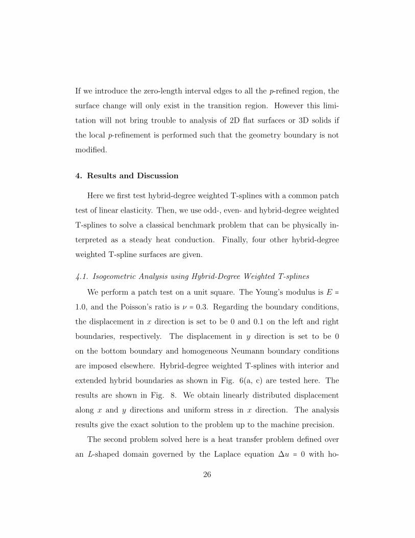
surfaces as shown in Fig. 11.
A square model is shown in Fig. 10(a), with a combination of degrees
2, 3, 4 and 5 basis functions, marked with different colors. Extended hy-
brid boundaries exist in this model. Hybrid-degree weighted T-splines can
combine basis functions of different degrees using different layers of transi-
tion regions. In Fig. 10(b), a circle model is provided with a combination
of degrees 3, 4 and 5 basis functions. Interior hybrid boundaries exist in
this model. There are 4 valance-3 extraordinary nodes. T-splines of p = 3 are
used to handle the extraordinary nodes. After local p-refinement with hybrid-
degree weighted T-splines, the surface is changed along the radial direction
29

(a) (b)
Figure 10: Open surface hybrid-degree weighted T-spline models. (a) A square model with
extended hybrid boundaries and the difference before (white lines) and after refinement
(black lines); and (b) a circle model with interior hybrid boundaries and the difference
before (white lines) and after refinement (black lines).
near the hybrid boundaries. In Fig. 10, the white and black lines show the
difference before and after local p-refinement. For open surface models, with
the scheme to calculate the control points, the local region around the hybrid
boundaries in the interior of the geometry is changed. The boundary of the
geometry remains unchanged after refinement.
Two closed surface models with extraordinary nodes are given in Fig. 11.
The Tetra model in Fig. 11(a) has eight valance-6 extraordinary nodes. The
original T-spline surface is of degree 3. After local p-refinement, the hybrid-
degree weighted T-spline is shown in Fig. 11(b), with the comparison before
and after refinement. Fig. 11(d-f) shows the Genus-three model before and
after local p-refinement. In this model, we set the two-ring neighborhood of
the four valance-8 extraordinary nodes as degree 3. For all the other regions,
the surface is of degree 4. With hybrid-degree weighted T-splines, we can
generate T-spline surfaces with basis functions of different degrees in one
30
(a) (b) (c)
(d) (e) (f)
Figure 11: Tetra model (a-c) and Genus-three model (d-f) of hybrid-degree weighted T-
splines. (a, d) Original model of degree 3; (b, e) local p-refinement results, where the
white and black lines show the difference of Bezier elements before and after refinement;
and (c, f) show the zoom-in of (b, e).
model.
5. Conclusions and Future Work
In conclusion, in this paper we develop a new algorithm to generate
hybrid-degree weighted T-splines which can be used in isogeometric anal-
ysis. Weighted T-splines of arbitrary degree are proposed which satisfy all
the analysis-suitable requirements. Hybrid-degree weighted T-splines are de-
veloped with two types of hybrid boundaries for local p-refinement. Both
odd- and even-degree T-spline basis functions are defined. The p-refined
regions and unchanged regions are connected via transition regions. Both
31
p-refined basis functions and original basis functions have support over the
transition regions, over which the hybrid-degree weighted T-splines are de-
fined. The transition region has basis functions of the same degree as the
p-refined region, and the same surface continuity as the unchanged region.
Bezier elements of different degrees are extracted for isogeometric analysis.
The Laplace equation is solved on an L-shaped domain, which is parameter-
ized with odd-, even-, and hybrid-degree T-splines. Hybrid T-splines provide
better performance after local p-refinement. In the future, we are planning to
develop a better control point calculation algorithm to decrease the surface
change after local p-refinement.
Acknowledgements
Lei Liu and Yongjie Jessica Zhang were supported in part by the PECASE
Award N00014-14-1–0234. Hugo Casquero and Hector Gomez were partially
supported by the European Research Council through the FP7 Ideas Start-
ing Grant (project # 307201). Hector Gomez was also partially supported
by Ministerio de Econoıa y Competitividad (project # DPI2013-44406-R),
confinanced with FEDER funds.
References
[1] T. J. R. Hughes, J. A. Cottrell, Y. Bazilevs, Isogeometric analysis: CAD,
finite elements, NURBS, exact geometry, and mesh refinement, Com-
puter Methods in Applied Mechanics and Engineering 194 (2005) 4135–
4195.
32
[2] L. A. Piegl, W. Tiller, The NURBS Book, 2nd ed., Springer-Verlag, New
York, 1997.
[3] J. A. Cottrell, T. J. R. Hughes, Y. Bazilevs, Isogeometric analysis: to-
ward integration of CAD and FEA, Wiley, 2009.
[4] G. Xu, B. Mourrain, R. Duvigneau, A. Galligo, Analysis-suitable volume
parameterization of multi-block computational domain in isogeometric
applications, Computer-Aided Design 45 (2) (2013) 395–404.
[5] T. W. Sederberg, J. Zheng, A. Bakenov, A. Nasri, T-splines and T-
NURCCs, ACM Transactions on Graphics 22 (3) (2003) 477–484.
[6] Y. Bazilevs, V. M. Calo, J. A. Cottrell, J. A. Evans, T. J. R. Hughes,
S. Lipton, M. A. Scott, T. W. Sederberg, Isogeometric analysis using
T-splines, Computer Methods in Applied Mechanics and Engineering
199 (5-8) (2010) 229–263.
[7] H. Casquero, L. Liu, Y. Zhang, A. Reali, H. Gomez, Isogeometric collo-
cation using analysis-suitable T-splines of arbitrary degree, submitted,
2015.
[8] S. Lipton, J. A. Evans, Y. Bazilevs, T. Elguedj, T. J. R. Hughes, Ro-
bustness of isogeometric structural discretizations under severe mesh
distortion, Computer Methods in Applied Mechanics and Engineering
199 (58) (2010) 357–373.
[9] I. Akkerman, Y. Bazilevs, V. M. Calo, T. J. R. Hughes, S. Hulshoff,
The role of continuity in residual-based variational multiscale modeling
of turbulence, Computational Mechanics 41 (2008) 371–378.
33

[10] Y. Bazilevs, V. M. Calo, T. J. R. Hughes, Y. Zhang, Isogeometric fluid-
structure interaction: theory, algorithms, and computations, Computa-
tional Mechanics 43 (1) (2008) 3–37.
[11] Y. Zhang, Y. Bazilevs, S. Goswami, C. L. Bajaj, T. J. R. Hughes,
Patient-specific vascular NURBS modeling for isogeometric analysis of
blood flow, Computer Methods in Applied Mechanics and Engineering
196 (29-30) (2007) 2943–2959.
[12] Y. Bazilevs, V. M. Calo, Y. Zhang, T. J. R. Hughes, Isogeometric fluid-
structure interaction analysis with applications to arterial blood flow,
Computational Mechanics 38 (4-5) (2006) 310–322.
[13] Y. Bazilevs, M.-C. Hsu, I. Akkerman, S. Wright, K. Takizawa,
B. Henicke, T. Spielman, T. Tezduyar, 3D simulation of wind turbine
rotors at full scale. part I: Geometry modeling and aerodynamics, Inter-
national Journal for Numerical Methods in Fluids 65 (2011) 207–235.
[14] Y. Bazilevs, M.-C. Hsu, J. Kiendl, R. Wuchner, K.-U. Bletzinger, 3D
simulation of wind turbine rotors at full scale. part II: Fluid-structure
interaction modeling with composite blades, International Journal for
Numerical Methods in Fluids 65 (2011) 236–253.
[15] J. Bueno, C. Bona-Casas, Y. Bazilevs, H. Gomez, Interaction of complex
fluids and solids: theory, algorithms and application to phase-change-
driven implosion, Computational Mechanics 55 (6) (2015) 1105–1118.
[16] D. Kamensky, M.-C. Hsu, D. Schillinger, J. A. Evans, A. Aggarwal,
Y. Bazilevs, M. S. Sacks, T. J. R. Hughes, An immersogeometric vari-
34

ational framework for fluid-structure interaction: application to bio-
prosthetic heart valves, Computer Methods in Applied Mechanics and
Engineering 284 (2015) 1005–1053.
[17] M.-C. Hsu, D. Kamensky, Y. Bazilevs, M. S. Sacks, T. J. R. Hughes,
Fluid-structure interaction analysis of bioprosthetic heart valves: signif-
icance of arterial wall deformation, Computational Mechanics 54 (2014)
1055–1071.
[18] M.-C. Hsu, D. Kamensky, F. Xu, J. Kiendl, C. Wang, M. Wu,
J. Mineroff, A. Reali, Y. Bazilevs, M. S. Sacks, Dynamic and fluid-
structure interaction simulations of bioprosthetic heart valves using
parametric design with T-splines and Fung-type material models, Com-
putational Mechanics 55 (2015) 1211–1225.
[19] H. Casquero, C. Bona-Casas, H. Gomez, A NURBS-based immersed
methodology for fluid-structure interaction, Computer Methods in Ap-
plied Mechanics and Engineering 284 (0) (2015) 943–970.
[20] H. Casquero, L. Liu, C. Bona-Casas, Y. Zhang, H. Gomez, A hybrid
variational-collocation immersed method for fluid-structure interaction
using unstructured T-splines, International Journal for Numerical Meth-
ods in Engineering (2015) doi:10.1002/nme.5004.
[21] H. Gomez, V. M. Calo, Y. Bazilevs, T. J. R. Hughes, Isogeometric anal-
ysis of the Cahn-Hilliard phase-field model, Computer Methods in Ap-
plied Mechanics and Engineering 197 (49-50) (2008) 4333–4352.
35

[22] H. Gomez, T. J. R. Hughes, X. Nogueira, V. M. Calo, Isogeometric
analysis of the isothermal Navier-Stokes-Korteweg equations, Computer
Methods in Applied Mechanics and Engineering 199 (2010) 1828–1840.
[23] J. Kiendl, K.-U. Bletzinger, J. Linhard, R. Wuchner, Isogeometric shell
analysis with Kirchhoff-Love elements, Computer Methods in Applied
Mechanics and Engineering 198 (2009) 3902–3914.
[24] J. Kiendl, M.-C. Hsu, M. C. H. Wu, A. Reali, Isogeometric Kirchhoff-
Love shell formulations for general hyperelastic materials, Computer
Methods in Applied Mechanics and Engineering 291 (2015) 280–303.
[25] H. Gomez, X. Nogueira, An unconditionally energy-stable method for
the phase field crystal equation, Computer Methods in Applied Mechan-
ics and Engineering 249 (2012) 52–61.
[26] G. Vilanova, I. Colominas, H. Gomez, Capillary networks in tumor an-
giogenesis: From discrete endothelial cells to phase-field averaged de-
scriptions via isogeometric analysis, International Journal for Numerical
Methods in Biomedical Engineering 29 (2013) 1015–1037.
[27] G. Vilanova, I. Colominas, H. Gomez, Coupling of discrete random walks
and continuous modeling for three-dimensional tumor-induced angiogen-
esis, Computational Mechanics 53 (2013) 449–464.
[28] F. Auricchio, L. B. Da Veiga, T. J. R. Hughes, A. Reali, G. Sanglli,
Isogeometric collocation methods, Mathematical Models and Methods
in Applied Sciences 20 (11) (2010) 2075–2107.
36
[29] D. Schillinger, J. A. Evans, A. Reali, M. A. Scott, T. J. R. Hughes,
Isogeometric collocation: cost comparison with Galerkin methods and
extension to adaptive hierarchical NURBS discretizations, Computer
Methods in Applied Mechanics and Engineering 267 (0) (2013) 170–232.
[30] H. Gomez, A. Reali, G. Sangalli, Accurate, efficient, and
(iso)geometrically flexible collocation methods for phase-field models,
Journal of Computational Physics 262 (2014) 153–171.
[31] A. Reali, H. Gomez, An isogeometric collocation approach for Bernoulli-
Euler beams and Kirchhoff plates, Computer Methods in Applied Me-
chanics and Engineering 284 (2015) 623–636.
[32] C. Anitescu, Y. Jia, Y. Zhang, T. Rabczuk, An isogeometric collocation
method using superconvergent points, Computer Methods in Applied
Mechanics and Engineering 284 (2015) 1073–1097.
[33] X. Li, M. A. Scott, Analysis-suitable T-splines: characterization, re-
fineability, and approximation, Mathematical Models and Methods in
Applied Sciences 24 (06) (2014) 1141–1164.
[34] X. Li, Some properties for analysis-suitable T-splines, Journal of Com-
putational Mathematics 33 (4) (2015) 428–442.
[35] A. Buffa, D. Cho, G. Sangalli, Linear independence of the T-spline
blending functions associated with some particular T-meshes, Com-
puter Methods in Applied Mechanics and Engineering 199 (23-24) (2010)
1437–1445.
37

[36] X. Li, J. Zheng, T. W. Sederberg, T. J. R. Hughes, M. A. Scott, On
linear independence of T-spline blending functions, Computer Aided
Geometric Design 29 (1) (2012) 63–76.
[37] L. Beirao da Veiga, A. Buffa, G. Sangalli, R. Vazquez, Analysis-suitable
T-splines of arbitrary degree: definition, linear independence and ap-
proximation properties, Mathematical Models and Methods in Applied
Sciences 23 (11) (2013) 1979–2003.
[38] A. Bressan, A. Buffa, G. Sangalli, Characterization of analysis-
suitable T-splines, Computer Aided Geometric Design (2015)
doi:10.1016/j.cagd.2015.06.007.
[39] M. A. Scott, R. N. Simpson, J. A. Evans, S. Lipton, S. P. A. Bor-
das, T. J. R. Hughes, T. W. Sederberg, Isogeometric boundary element
analysis using unstructured T-splines, Computer Methods in Applied
Mechanics and Engineering 254 (0) (2013) 197–221.
[40] L. Liu, Y. Zhang, X. Wei, Weighted T-splines with application in repa-
rameterizing trimmed NURBS surfaces, Computer Methods in Applied
Mechanics and Engineering 295 (2015) 108–126.
[41] L. Liu, Y. Zhang, X. Wei, Handling extraordinary nodes with weighted
T-spline basis functions, in: 24th International Meshing Roundtable,
accepted, 2015.
[42] T. W. Sederberg, D. L. Cardon, G. T. Finnigan, N. S. North, J. Zheng,
T. Lyche, T-spline simplification and local refinement, in: ACM SIG-
GRAPH, 2004, pp. 276–283.
38

[43] M. A. Scott, X. Li, T. W. Sederberg, T. J. R. Hughes, Local refinement
of analysis-suitable T-splines, Computer Methods in Applied Mechanics
and Engineering 213-216 (0) (2012) 206–222.
[44] P. Morgenstern, D. Peterseim, Analysis-suitable adaptive T-mesh refine-
ment with linear complexity, Computer Aided Geometric Design 34 (0)
(2015) 50–66.
[45] P. Morgenstern, 3D Analysis-suitable T-splines: definition, lin-
ear independence and m-graded local refinement (2015), ArXiv e-
printsarXiv:1505.05392, 2015.
[46] E. J. Evans, M. A. Scott, X. Li, D. C. Thomas, Hierarchical T-splines:
Analysis-suitability, Bezier extraction, and application as an adaptive
basis for isogeometric analysis, Computer Methods in Applied Mechan-
ics and Engineering 284 (2015) 1–20.
[47] C. Giannelli, B. Juttler, H. Speleers, THB-splines: the truncated basis
for hierarchical splines, Computer Aided Geometric Design 29 (2012)
485–498.
[48] X. Wei, Y. Zhang, T. J. R. Hughes, M. A. Scott, Truncated hierarchi-
cal Catmull-Clark surface with local refinement, Computer Methods in
Applied Mechanics and Engineering 291 (2015) 1–20.
[49] X. Wei, Y. Zhang, T. J. R. Hughes, M. A. Scott, Extended truncated
hierarchical Catmull-Clark subdivision, Computer Methods in Applied
Mechanics and Engineering, accepted, 2015.
39

[50] H. Prautzsch, Degree elevation of B-spline curves, Computer Aided Ge-
ometric Design 1 (2) (1984) 193–198.
[51] E. Cohen, T. Lyche, L. L. Schumaker, Algorithms for degree-raising of
splines, ACM Transactions on Graphics 4 (3) (1985) 171–181.
[52] E. Cohen, T. Lyche, L. L. Schumaker, Degree raising for splines, Journal
of Approximation Theory 46 (2) (1986) 170–181.
[53] H. Prautzsch, B. Piper, A fast algorithm to raise the degree of spline
curves, Computer Aided Geometric Design 8 (4) (1991) 253–265.
[54] L. Piegl, W. Tiller, Software-engineering approach to degree elevation
of B-spline curves, Computer-Aided Design 26 (1) (1994) 17–28.
[55] T. W. Sederberg, J. Zheng, X. Song, Knot intervals and multi-degree
splines, Computer Aided Geometric Design 20 (7) (2003) 455–468.
[56] W. Shen, G. Wang, A basis of multi-degree splines, Computer Aided
Geometric Design 27 (1) (2010) 23–35.
[57] X. Li, Z. Huang, Z. Liu, A geometric approach for multi-degree spline,
Journal of Computer Science and Technology 27 (4) (2012) 841–850.
[58] M. A. Scott, M. J. Borden, C. V. Verhoosel, T. W. Sederberg, T. J. R.
Hughes, Isogeometric finite element data structures based on Bezier ex-
traction of T-splines, International Journal for Numerical Methods in
Engineering 88 (2) (2011) 126–156.
40

[59] R. Goldman, T. Lyche, Knot insertion and deletion algorithms for
B-spline curves and surfaces, Society for Industrial and Applied
Mathematics–Philadelphia, 1993.
[60] W. Wang, Y. Zhang, G. Xu, T. J. R. Hughes, Converting an unstruc-
tured quadrilateral/hexahedral mesh to a rational T-spline, Computa-
tional Mechanics 50 (1) (2012) 65–84.
[61] S. Giani, P. Houston, Anisotropic hp-adaptive discontinuous galerkin
finite element methods for compressible fluid flows, International Journal
of Numerical Analysis and Modeling 9 (4) (2012) 928–949.
41


