
Heritability, OPERA and ICE FALCON: thoughts on causation, and causes of variation
in (some aspect of a) disease
John Hopper
Melbourne School of Population and Global Health
The University of Melbourne

SBS Insight March 2016

Heritability is not the proportion disease due to genes
Many (mis)interpret it this way
Tomlinson et al. A genome-wide association study identifies colorectal cancer susceptibility loci on chromosomes 10p14 and 8q23.3. Nat Genet 2008;40:623-30.
Characteristic of a population in fixed environment
Crude measure of the impact of genes on variation,
not on cause per se
Heritability: what it isn’t
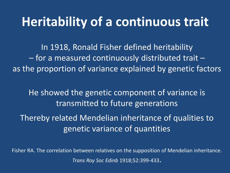
Heritability of a continuous trait
In 1918, Ronald Fisher defined heritability – for a measured continuously distributed trait –
as the proportion of variance explained by genetic factors
He showed the genetic component of variance is transmitted to future generations
Thereby related Mendelian inheritance of qualities to genetic variance of quantities
Fisher RA. The correlation between relatives on the supposition of Mendelian inheritance.
Trans Roy Soc Edinb 1918;52:399-433.

Hotch-potch of a denominator
Fisher showed that it was the absolute genetic variance, not a percentage, that was important
Fisher referred to the total variance as a “hotch-potch of a denominator”
He admonished that:
"loose phrases about the "percentage of causation", which obscure the essential distinction
between the individual and the population, should be carefully avoided"
Fisher RA. Limits to intensive production in animals. Brit Agric Bull 1951;4:217-218.
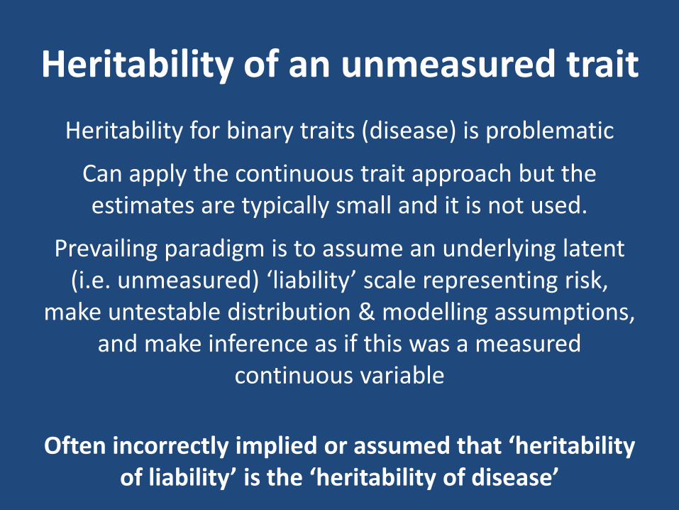
Heritability of an unmeasured trait
Heritability for binary traits (disease) is problematic
Can apply the continuous trait approach but the estimates are typically small and it is not used.
Prevailing paradigm is to assume an underlying latent (i.e. unmeasured) ‘liability’ scale representing risk,
make untestable distribution & modelling assumptions, and make inference as if this was a measured
continuous variable
Often incorrectly implied or assumed that ‘heritability of liability’ is the ‘heritability of disease’

Liability model
• Witte et al?
Witte, Visscher & Wray. The contribution of genetic variants to disease depends on the ruler. Nat Rev Genet. 2014;15:765-76.
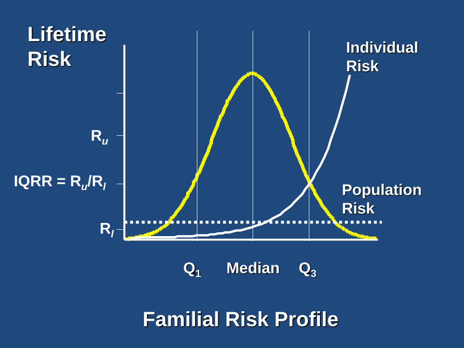
Familial Risk Profile
Q1 Q3
Ru
Rl
Median
Population
Risk
Individual
Risk
Lifetime
Risk
IQRR = Ru/Rl
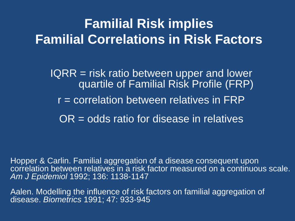
Familial Risk implies
Familial Correlations in Risk Factors
IQRR = risk ratio between upper and lower quartile of Familial Risk Profile (FRP)
r = correlation between relatives in FRP
OR = odds ratio for disease in relatives
Hopper & Carlin. Familial aggregation of a disease consequent upon correlation between relatives in a risk factor measured on a continuous scale. Am J Epidemiol 1992; 136: 1138-1147
Aalen. Modelling the influence of risk factors on familial aggregation of disease. Biometrics 1991; 47: 933-945

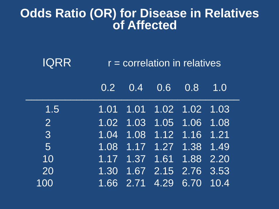
Odds Ratio (OR) for Disease in Relatives of Affected
IQRR r = correlation in relatives
0.2 0.4 0.6 0.8 1.0 ______________________________________
1.5 1.01 1.01 1.02 1.02 1.03
2 1.02 1.03 1.05 1.06 1.08
3 1.04 1.08 1.12 1.16 1.21
5 1.08 1.17 1.27 1.38 1.49
10 1.17 1.37 1.61 1.88 2.20
20 1.30 1.67 2.15 2.76 3.53
100 1.66 2.71 4.29 6.70 10.4
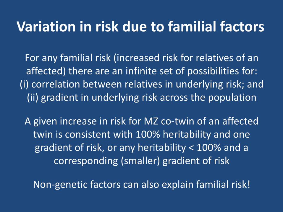
Variation in risk due to familial factors
For any familial risk (increased risk for relatives of an affected) there are an infinite set of possibilities for:
(i) correlation between relatives in underlying risk; and (ii) gradient in underlying risk across the population
A given increase in risk for MZ co-twin of an affected twin is consistent with 100% heritability and one gradient of risk, or any heritability < 100% and a
corresponding (smaller) gradient of risk
Non-genetic factors can also explain familial risk!

… unmeasured non-familial factors?
All depends on the variation in risk explained by non-familial factors, which could vary across populations and time, and be more than just
what is known to date for measured ‘environmental’ factors
Denominator is not so much a “hotch-potch”,
it is simply unknowable!

Why ‘all-or-nothing’ liability assumption?
All-or-nothing assumption of the liability model - risk is 100% for those above a given threshold -
is arbitrary
There are no degrees of freedom to test this assumption!
Hardly a basis for a scientific theory

What if another liability assumption?
Different scenarios give different correlations in liability
e.g. prevalence = 10% and ORMZ = 5
Proportion above threshold at risk Correlation in liability
100% 0.5
50% 0.3
25% 0.1
Heritability estimates depend greatly on the assumed liability model

Conclusion
Estimates of the “heritability of liability” rely on distributional and other untested assumptions
and are not statistically robust
Not a sound scientific construct
Estimates of the “heritability of a disease” are virtually meaningless
It suggests “proportion of disease due to genes”
This not correct, no matter what model is assumed

Comparing risk factors gradients
measured on different scales
using
Odds PER Adjusted
standard deviation
(OPERA)

Inspired by Mammographic Density
• (P)MD is “second to BRCA1/2” … but is it?
• Binary versus continuous
• (P)MD is not the risk factor, it is (P)MD for age and BMI
• OPERA is a unifying concept …
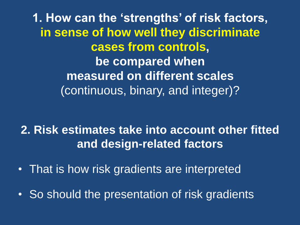
1. How can the ‘strengths’ of risk factors,
in sense of how well they discriminate
cases from controls,
be compared when
measured on different scales
(continuous, binary, and integer)?
2. Risk estimates take into account other fitted
and design-related factors
• That is how risk gradients are interpreted
• So should the presentation of risk gradients

Odds PER Adjusted standard deviation
(OPERA)
• For risk factor X0, derive best fitting relationship between mean of X0 and all other covariates fitted in the model or adjusted for by design
(X1, X2, …, Xn)
OPERA presents risk association for X0
in terms of change in risk per
standard deviation of X0 adjusted for X1, X2, …, Xn,
rather than standard deviation of X0 itself.

Binary Risk Factors
• For binary factor with prevalence p,
s = [p(1-p)]0.5
• A = 1/s is the number of standard deviations between the two outcomes
• Risk increases RR-fold over A standard deviations
OPERA = exp [ln(RR)/A]= RRs

Sex/gender
• Binary (0 = male, 1 = female); p = 0.5
• Assume RR = 100, say
• Standard deviation s = [p(1-p)]0.5 = 0.5 (i.e. A = 2)
• OPERA = exp [ln(100)/2)] = 1000.5 = 10
• Change from 0 to 1 is A = 2 standard deviations
• Odds increase by 100 over two standard deviations
• So increases 10-fold over one standard deviation
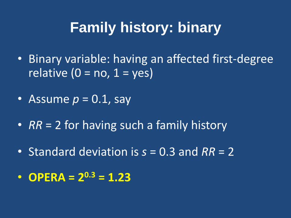
Family history: binary
• Binary variable: having an affected first-degree relative (0 = no, 1 = yes)
• Assume p = 0.1, say
• RR = 2 for having such a family history
• Standard deviation is s = 0.3 and RR = 2
• OPERA = 20.3 = 1.23
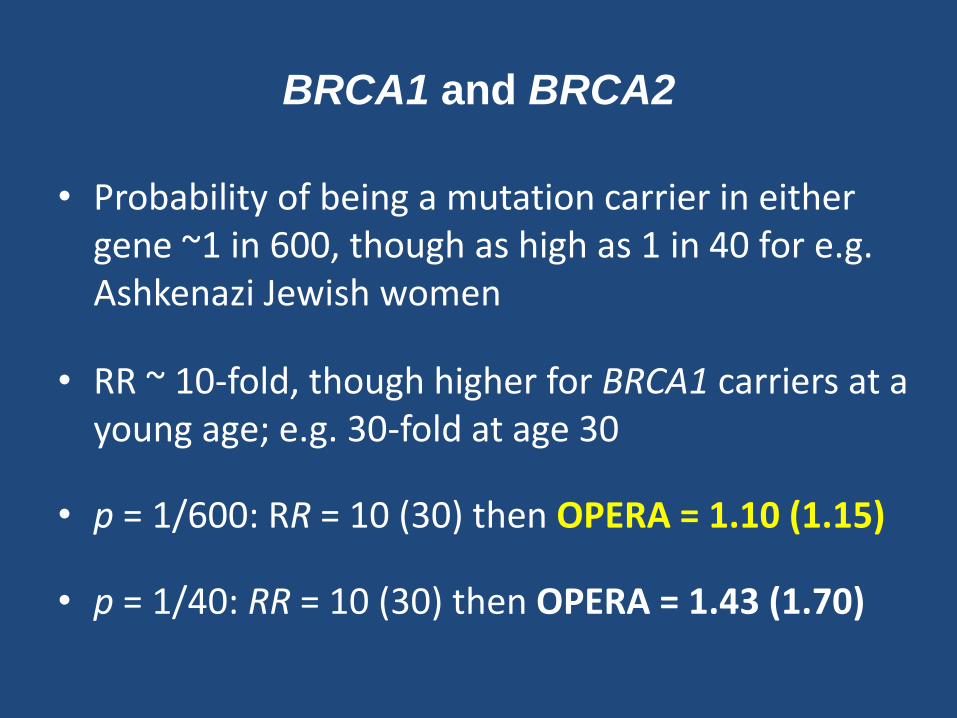
BRCA1 and BRCA2
• Probability of being a mutation carrier in either gene ~1 in 600, though as high as 1 in 40 for e.g. Ashkenazi Jewish women
• RR ~ 10-fold, though higher for BRCA1 carriers at a young age; e.g. 30-fold at age 30
• p = 1/600: RR = 10 (30) then OPERA = 1.10 (1.15)
• p = 1/40: RR = 10 (30) then OPERA = 1.43 (1.70)
Odds Ratio (OR) for Disease in Relatives of Affected
IQRR r = correlation in relatives
0.2 0.4 0.6 0.8 1.0 ______________________________________
1.5 1.01 1.01 1.02 1.02 1.03
2 1.02 1.03 1.05 1.06 1.08
3 1.04 1.08 1.12 1.16 1.21
5 1.08 1.17 1.27 1.38 1.49
10 1.17 1.37 1.61 1.88 2.20
20 1.30 1.67 2.15 2.76 3.53
100 1.66 2.71 4.29 6.70 10.4

All familial factors
• Multitude of familial factors explain 2-fold increased risk for having affected 10 relative
• Under a multiplicative polygenic model, interquartile risk ratio ~20-fold
• Mean upper quartile of normal distribution is 1.27 SD
• 20-fold increased risk across 2.54 standard deviations: IQRR = OPERA2.54
• OPERA = 3.25
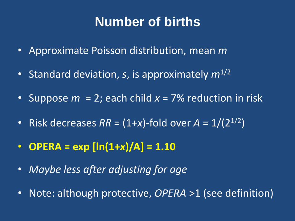
Number of births
• Approximate Poisson distribution, mean m
• Standard deviation, s, is approximately m1/2
• Suppose m = 2; each child x = 7% reduction in risk
• Risk decreases RR = (1+x)-fold over A = 1/(21/2)
• OPERA = exp [ln(1+x)/A] = 1.10
• Maybe less after adjusting for age
• Note: although protective, OPERA >1 (see definition)
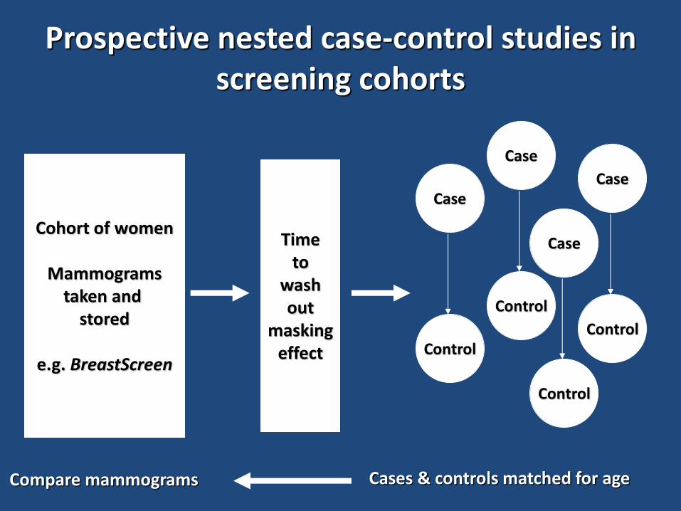
Prospective nested case-control studies in screening cohorts
Cohort of women
Mammograms taken and
stored
e.g. BreastScreen
Case
Control
Case
Control
Case
Control
Time to
wash out
masking effect
Cases & controls matched for age Compare mammograms
Case
Control
perc
en
tage d
ensity
age at mammogram - yrs 40 50 60 70
0
10
20
30
40
50
60
70
80
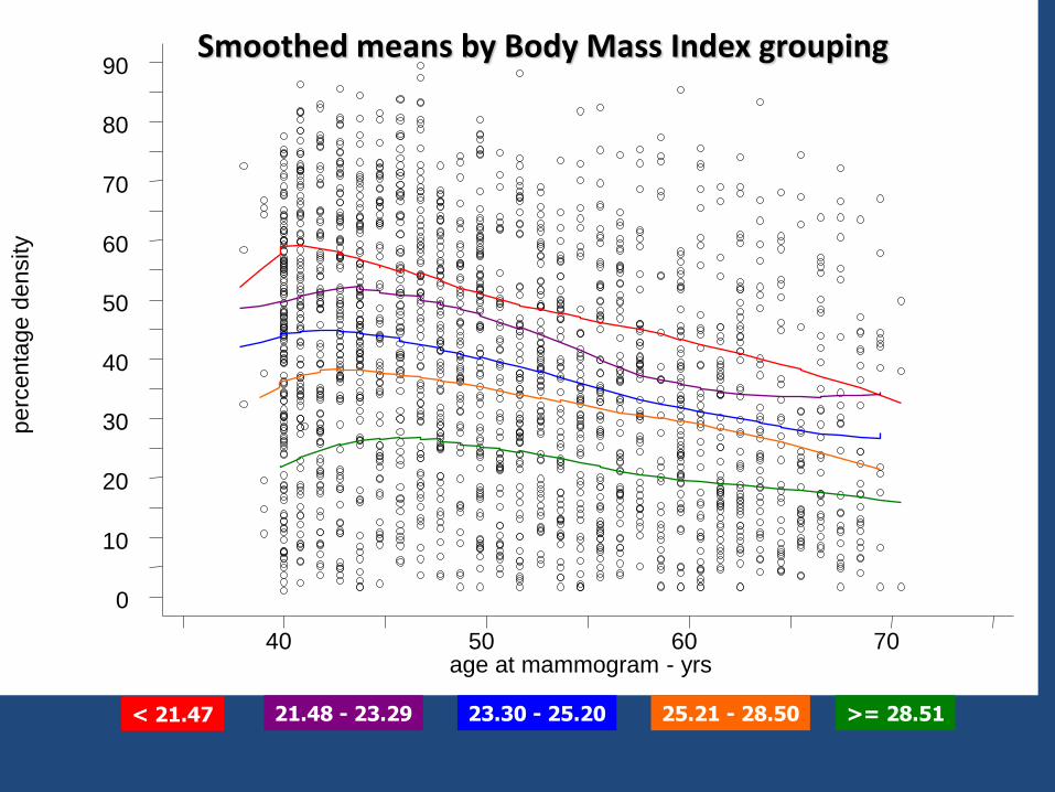
90 Smoothed means by Body Mass Index grouping
< 21.47 21.48 - 23.29 23.30 - 25.20 25.21 - 28.50 >= 28.51
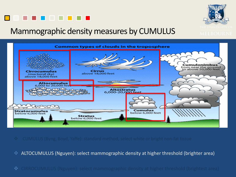
CUMULUS (Byng, Boyd, Yaffe): standard method, select white or bright non-fat tissue
ALTOCUMULUS (Nguyen): select mammographic density at higher threshold (brighter area)
CIRROCUMULUS (Nguyen): select mammographic density at higher threshold (brightest area)
Mammographic density measures by CUMULUS

Mammographic density measures by CUMULUS
Cumulus: Dense Area =331,976 pixels Percent Density =26.77%
Altocumulus: Dense Area =123,041 pixels Percent Density =9.92% Correlation with Cumulus =0.8
Cirrocumulus: Dense Area =12,986 pixels Percent Density = 1.05% Correlation with Cumulus =0.6
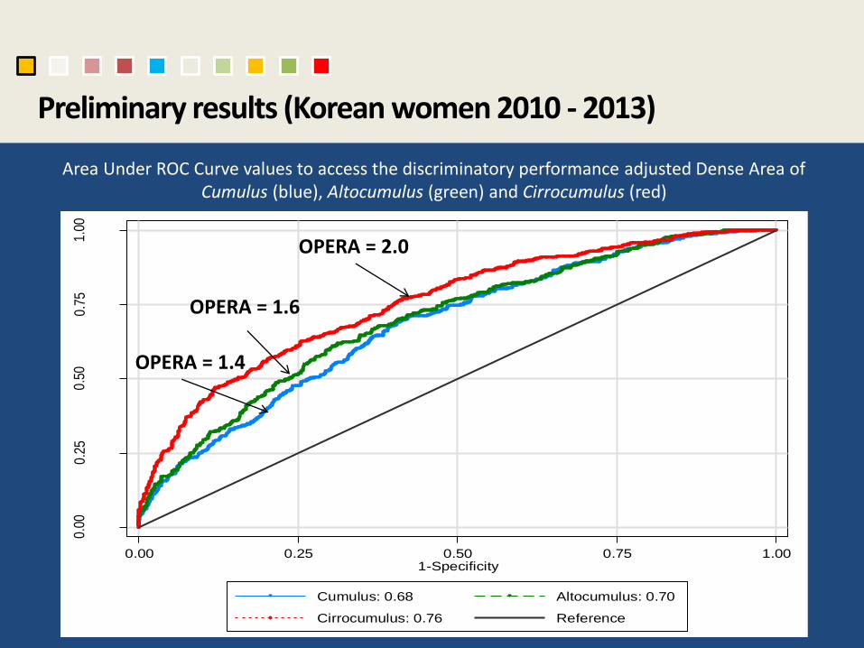
Preliminary results (Korean women 2010 - 2013) 0
.00
0.2
50
.50
0.7
51
.00
Se
nsiti
vity
0.00 0.25 0.50 0.75 1.001-Specificity
Cumulus: 0.68 Altocumulus: 0.70
Cirrocumulus: 0.76 Reference
Area Under ROC Curve values to access the discriminatory performance adjusted Dense Area of Cumulus (blue), Altocumulus (green) and Cirrocumulus (red)
OPERA = 2.0
OPERA = 1.6
OPERA = 1.4
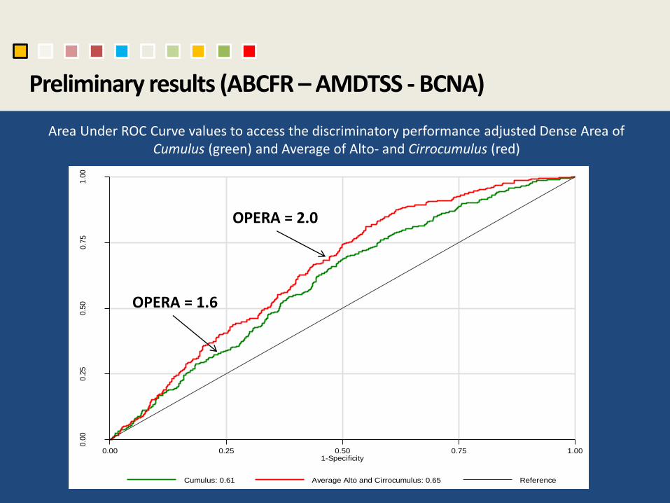
Preliminary results (ABCFR – AMDTSS - BCNA)
Area Under ROC Curve values to access the discriminatory performance adjusted Dense Area of Cumulus (green) and Average of Alto- and Cirrocumulus (red)
0.0
00.2
50.5
00.7
51.0
0
Sensi
tivity
0.00 0.25 0.50 0.75 1.001-Specificity
Cumulus: 0.61 Average Alto and Cirrocumulus: 0.65 Reference
OPERA = 2.0
OPERA = 1.6

Mammographic Density
• Mammographic density - white or bright areas on a mammogram – adjusted for age and BMI
• Observations show that the OPERA ~ 1.40
• Novel approaches to extracting more information on risk from mammograms, are proving to be even better risk predictors
• OPERA as high as 2.0
• These are not as familial (e.g. rMZ = 0.2 cf. 0.6)
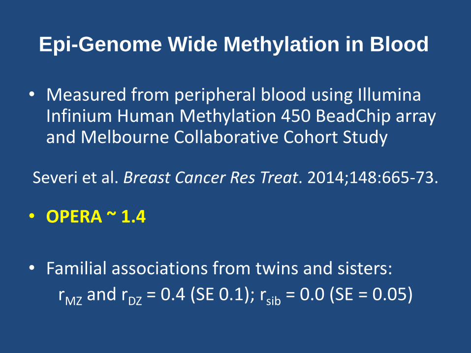
Epi-Genome Wide Methylation in Blood
• Measured from peripheral blood using Illumina Infinium Human Methylation 450 BeadChip array and Melbourne Collaborative Cohort Study
Severi et al. Breast Cancer Res Treat. 2014;148:665-73.
• OPERA ~ 1.4
• Familial associations from twins and sisters:
rMZ and rDZ = 0.4 (SE 0.1); rsib = 0.0 (SE = 0.05)

Single Nucleotide Polymorphisms (SNPs)
• Common genetic markers
• SNPs associated with risk are being found
• Currently 77 independent common genetic markers known to predict breast cancer risk explain ~14% of familial aggregation
• OPERA = 1.56 overall; 1.6 for ER+ve and 1.4 for ER-ve disease, reflecting sampling

0.0
00
.25
0.5
00
.75
1.0
0
Se
nsitiv
ity
0.00 0.25 0.50 0.75 1.00
1-Specificity
BOADICEA and SNP-based
BOADICEA
SNP-based
Reference
BOADICEA and SNP score adjusted for age
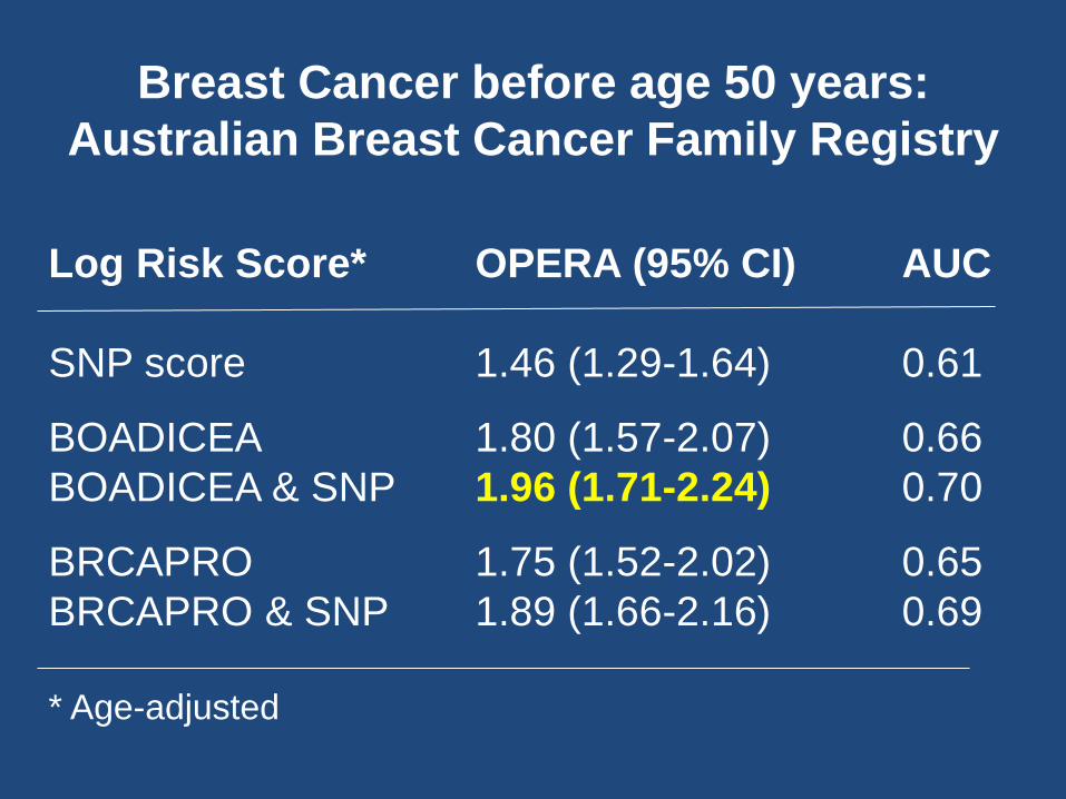
Breast Cancer before age 50 years:
Australian Breast Cancer Family Registry
Log Risk Score* OPERA (95% CI) AUC
SNP score 1.46 (1.29-1.64) 0.61
BOADICEA 1.80 (1.57-2.07) 0.66
BOADICEA & SNP 1.96 (1.71-2.24) 0.70
BRCAPRO 1.75 (1.52-2.02) 0.65
BRCAPRO & SNP 1.89 (1.66-2.16) 0.69
* Age-adjusted

OPERA scores for breast cancer
Risk factor OPERA Comment
Gender 10
Age ? Depends on ages
All familial causes >3 Known and unknown
Mammographic density 1.4-2.0 Likely to increase
Family history models 1.8 Multi-generations
Known polygenic markers 1.6 Likely to increase
Global methylation 1.4 Not highly familial
Known gene mutations 1.2-1.7 Depends on age/ethnicity
Family history 1.2 First-degree only; yes/no
Number of child births 1.1 Depends on family size
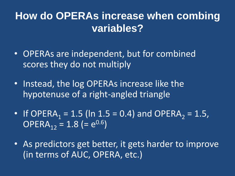
How do OPERAs increase when combing
variables?
• OPERAs are independent, but for combined scores they do not multiply
• Instead, the log OPERAs increase like the hypotenuse of a right-angled triangle
• If OPERA1 = 1.5 (ln 1.5 = 0.4) and OPERA2 = 1.5, OPERA12 = 1.8 (= e0.6)
• As predictors get better, it gets harder to improve (in terms of AUC, OPERA, etc.)

Putting risk gradients into perspective across diseases, populations and settings
• Risk gradients can be compared across – diseases
– sub-sets of a disease (e.g. based on age at onset or sub-type)
– populations and different environmental settings
• For any risk factor, rank the diseases to which it predisposes
• How changes in a risk factor impact on multiple diseases - for which disease(s) an intervention might have most impact
• Take into account benefits per disease (some might be negative) to see the overall impact of the intervention

Summary
• OPERA estimates are independent, by definition
(Of course, depend on sample and population)
• Compare predictive strengths of risk factors across:
–diseases
–populations, etc.
• OPERA principle also applies to hazard ratio (HR) estimates from cohort studies


