International Business & Economics Research Journal – May/June 2014 Volume 13, Number 3
Copyright by author(s); CC-BY 485 The Clute Institute
Hedge Fund Performance Evaluation Using
The Sharpe And Omega Ratios Francois van Dyk, UNISA, South Africa
Gary van Vuuren, North-West University, Potchefstroom Campus, South Africa
André Heymans, North-West University, Potchefstroom Campus, South Africa
ABSTRACT
The Sharpe ratio is widely used as a performance evaluation measure for traditional (i.e., long
only) investment funds as well as less-conventional funds such as hedge funds. Based on mean-
variance theory, the Sharpe ratio only considers the first two moments of return distributions, so
hedge funds – characterised by asymmetric, highly-skewed returns with non-negligible higher
moments – may be misdiagnosed in terms of performance. The Sharpe ratio is also susceptible to
manipulation and estimation error. These drawbacks have demonstrated the need for augmented
measures, or, in some cases, replacement fund performance metrics. Over the period January
2000 to December 2011 the monthly returns of 184 international long/short (equity) hedge funds
with geographical investment mandates spanning North America, Europe, and Asia were
examined. This study compares results obtained using the Sharpe ratio (in which returns are
assumed to be serially uncorrelated) with those obtained using a technique which does account for
serial return correlation. Standard techniques for annualising Sharpe ratios, based on monthly
estimators, do not account for this effect. In addition, this study assesses whether the Omega ratio
supplements the Sharpe Ratio in the evaluation of hedge fund risk and thus in the investment
decision-making process. The Omega and Sharpe ratios were estimated on a rolling basis to
ascertain whether the Omega ratio does indeed provide useful additional information to investors
to that provided by the Sharpe ratio alone.
Keywords: Hedge Funds; Omega Ratio; Sharpe Ratio; Risk Management
1. INTRODUCTION
ven before the advent of the first hedge fund structure by Alfred Winslow Jones in 1949 institutional
investors as well as wealthy individuals have been interested in hedge funds as early as the 1920s when
several private investment vehicles were available to wealthy investors. The public’s interest in these
funds has also increased through some extravagant hedge fund phenomena, such as the collapse of Long Term
Capital Management (LTCM)1 in the late 1990s, Amaranth Advisors
2 in 2006 and the Madoff Ponzi scheme
3 in late
2008. Since the early 1990s, hedge funds have become an increasingly popular asset class as global investment
increased from US$50bn in 1990 to US$2.2tn in early 2007 (Barclayhedge, 2013). Between 2003 and 2007 the
hedge fund industry posted its sturdiest gains, in terms of asset flows and performance whereafter the financial crisis
significantly curtailed growth. Due to substantial investor redemptions and performance-based declines industry
growth reversed, declining to US$1.4tn by April 2009 (Eurekahedge, 2012). Total assets under management (AUM)
1 A large US based hedge fund that nearly caused the collapse of the global financial system in 1998 due to high-risk arbitrage bond trading
strategies. The fund was highly leveraged when Russia defaulted on its debt causing a flight to quality. The fund suffered massive losses, and was
ultimately bailed out with the assistance of the Federal Reserve Bank and a consortium of banks. 2 To date, Amaranth Advisors marked the most significant loss of value for a hedge fund. The hedge fund attracted assets under management of
US$9bn whereafter faulty risk models and non-rebounding gas prices resulted in failure for the funds’ energy trading strategy as it lost US$6bn
on natural gas futures in 2006. Amaranth was also charged with the attempted manipulation of natural gas futures prices. Refer to Till (2007) for further details. 3 Considered the largest financial scandal in modern times with losses estimated at US$85bn, Madoff Securities LLC provided investors with
modest yet steady returns and claimed to be generating these returns by trading in S&P 500 index options employing an index arbitrage strategy. Madoff Securities did, however, commit fraud through a Ponzi scheme structure.
E

International Business & Economics Research Journal – May/June 2014 Volume 13, Number 3
Copyright by author(s); CC-BY 486 The Clute Institute
for the hedge fund industry has risen to only US$1.89tn by the end of June 2013 (Eurekahedge, 2013a) after posting
its first decline (US$2.94bn) of 2013 in June. The industry also suffered US$3.8tn of new outflows during 2012
(Eurekahedge, 2013b). Figure 1 presents the AUM for the hedge fund industry since 1997 until quarter 2 of 2013.
Figure 1: Hedge Funds' Assets under Management (US$tns) Since 1997
Source: Barclayhedge (2013)
The combination of a benevolent interest rate environment4 combined with indifferent regulatory scrutiny
along with a shortage in viable investment alternatives has promoted the growth of the hedge fund industry (Botha,
2007).
On top of their (net) assets size, hedge funds occupy a vital function in the global securities markets while
the hedge fund industry provides value to investors, markets and the broader economy. In terms of performance,
hedge funds deliver, on average, economically and statistically significant abnormal performance on both an equal-
and value-weighted basis and also across strategies, domiciles, size categories, and time-periods (Joenväärä et al.,
2012).5 Although there is evidence that hedge funds are affected by financial market stresses, there is no thorough
academic evidence that indicates that hedge funds cause economic instability. Furthermore, Getmansky et al. (2012)
found that hedge funds have exposure to systemic risk, but not that they contribute to it and that they suffer from,
rather than cause, forced liquidations. It could be argued that due to their essentially counter-cyclical nature hedge
funds in reality reduce instability and lessen systemic risk.
Hedge funds also contribute to the efficient functioning of financial markets as they are important providers
of liquidity in various financial markets while evidence also exists that hedge funds provide liquidity through short
sales. These funds are also responsible for improving price discovery and through both job creation6 and tax
revenues7 contribute to the broader economy. Also hedge funds employ substantial leverage (Malkiel & Saha,
2005), assume risks that other will not, mitigate price downturns and seek out inefficiencies (Botha, 2007). Apart
from the prospect of double- and triple-digit returns, investors are tempted to invest in hedge funds for the
persuasive motive that hedge fund returns seem uncorrelated with market indices; i.e., the broader market. This is
the rationale for the “hedge” in hedge funds: they enjoy relatively low correlations with traditional asset classes
(Fung & Hsieh, 1997) and so offer investors attractive diversification benefits for asset portfolios (Liang, 1999) (see
Figure 2). Survey results from SEI Knowledge Partnership showed that institutional investors are less interested on
4 Many hedge fund strategies rely on borrowed funds to leverage investment positions and so a kind interest rate environment is highly positive
(Botha, 2007). 5 Apart from average performance over a given time period it has recently been shown that hedge fund performance persists at annual horizons, while it was shown prior to only persist over quarterly horizons. 6 AIMA 2010 global survey indicated that world’s hedge fund industry employs an estimated 300,000 people (KPMG, 2012). 7 2009 survey by Open Europe found that the hedge fund and private equity industries contribute €9bn to the European Union in tax revenues. The survey estimated that in the UK alone the industry contributes £3.2bn to tax revenues (KPMG, 2012).
0.0
0.5
1.0
1.5
2.0
2.5
1997 Q1 1999 Q1 2001 Q1 2003 Q1 2005 Q1 2007 Q1 2009 Q1 2011 Q1 2013 Q1
Ass
ets
un
de
r m
anag
em
en
t (U
S$ t
ns)

International Business & Economics Research Journal – May/June 2014 Volume 13, Number 3
Copyright by author(s); CC-BY 487 The Clute Institute
achieving absolute returns than they are on capturing differentiated, non-correlated returns8 (SEI, 2013). These
alternative investments embrace a variety of different strategies, styles, and securities and hence the necessity for
risk management measures and techniques designed specifically for these funds is undeniable. In spite of the
promised diversification benefit on hand, these funds remain highly risky investments as stellar returns cannot be
obtained without significant risks (Botha, 2007).
Figure 2: Correlations between Hedge Funds and Main Asset Classes (Jan 1994 – Dec 2011)
Source: KPMG (2012). Global stocks = MSCI World Total Return Index, Global Bonds = JP Morgan Global Aggregate
Bond Total Return Index, Commodities = S&P GSCI Commodity Total Return Index. Hedge fund performance using HFR equal-weighted index and strategy indices.
While for the most part comparisons of hedge fund returns focus solely on total return values, comparing
funds in this manner that have dissimilar expected returns and risks is meaningless. The arrangement of risk and
return into a risk-adjusted number is one of the primary responsibilities of performance measurement (Lhabitant,
2004). A number of risk-adjusted9 performance measures (of which some are commonly used in traditional funds)
have been adopted by the hedge fund industry, such as the Sharpe and Treynor ratios, Jensen alpha, and
downside (risk) measures in the Sortino ratio, and Value-at-Risk (VaR).
Amongst hedge funds, the Sharpe ratio is the metric of choice and also the most commonly used measure
of risk-adjusted performance (Lhabitant, 2004; Opdyke, 2007; Schmid & Schmidt, 2007). Proposed by Sharpe as the
“reward-to-variability” ratio as a comparison tool for mutual funds (Sharpe, 1966, 1975, 1994) the ratio is
conceptually uncomplicated and also rich in meaning, providing investors with an objective, quantitative measure of
performance. The ratio benefits from widespread use and copious interpretations, but also has its shortcomings.
Being unsuitable for dealing with asymmetric return distributions are, among others a drawback of volatility
measures (Lhabitant, 2004).
The hedge fund universe witnessed an annual return of 8.82% between 1995 and 2003 compared to the
12.38% annual return for the S&P500 (Malkiel & Saha, 2005). More recently, in 2011 the hedge fund industry
reported a 4.6% loss with most losses occurring during the third quarter when global equity markets declines by
approximately 17% (TheCityUK, 2012). In 2012 the industry grew its total assets by US$64.5bn to reach US$1.77tn
while returns were also the lowest for a positive year, 6.12%, compared to the 13.75% return of the MSCI World
Index (Boyd, 2013). In the same year, launch activity slowed while the fund closure rate was the highest since the
financial crisis. Annual hedge fund launch and liquidation numbers from 2000 until Q1 2013 are presented in Figure
3.
8 Around 47% of senior investment professionals at 107 institutions surveyed rated diversification as their primary objective when investing in
hedge funds. 2nd placed objective = absolute returns (20%), 3rd = decreased volatility (13%). 9 Usually performance indicators that combine the returns with the risk of the fund (Botha, 2007).
-1
-0.5
0
0.5
1
All Hedge Funds
Equity Hedge
Emerging Markets
Event Driven
CTA and Macro
Relative Value
Market Neutral
Short Bias
Global Stocks
Global Bonds
Commodities
International Business & Economics Research Journal – May/June 2014 Volume 13, Number 3
Copyright by author(s); CC-BY 488 The Clute Institute
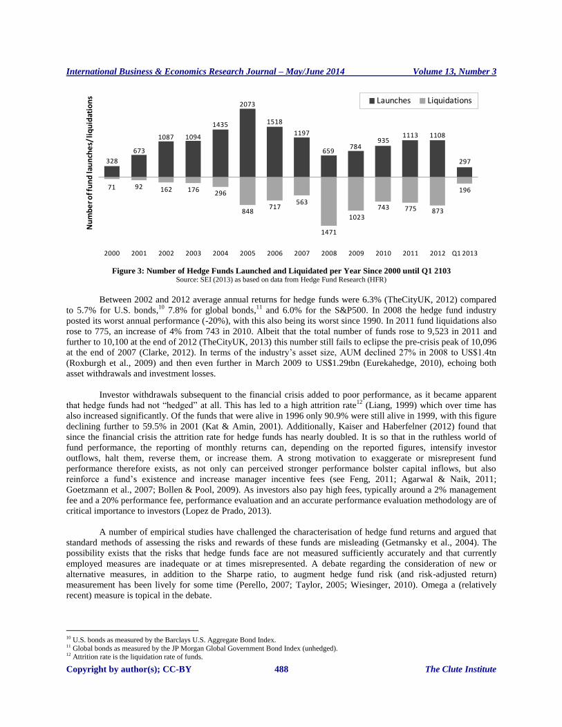
Figure 3: Number of Hedge Funds Launched and Liquidated per Year Since 2000 until Q1 2103
Source: SEI (2013) as based on data from Hedge Fund Research (HFR)
Between 2002 and 2012 average annual returns for hedge funds were 6.3% (TheCityUK, 2012) compared
to 5.7% for U.S. bonds,10
7.8% for global bonds,11
and 6.0% for the S&P500. In 2008 the hedge fund industry
posted its worst annual performance (-20%), with this also being its worst since 1990. In 2011 fund liquidations also
rose to 775, an increase of 4% from 743 in 2010. Albeit that the total number of funds rose to 9,523 in 2011 and
further to 10,100 at the end of 2012 (TheCityUK, 2013) this number still fails to eclipse the pre-crisis peak of 10,096
at the end of 2007 (Clarke, 2012). In terms of the industry’s asset size, AUM declined 27% in 2008 to US$1.4tn
(Roxburgh et al., 2009) and then even further in March 2009 to US$1.29tbn (Eurekahedge, 2010), echoing both
asset withdrawals and investment losses.
Investor withdrawals subsequent to the financial crisis added to poor performance, as it became apparent
that hedge funds had not “hedged” at all. This has led to a high attrition rate12
(Liang, 1999) which over time has
also increased significantly. Of the funds that were alive in 1996 only 90.9% were still alive in 1999, with this figure
declining further to 59.5% in 2001 (Kat & Amin, 2001). Additionally, Kaiser and Haberfelner (2012) found that
since the financial crisis the attrition rate for hedge funds has nearly doubled. It is so that in the ruthless world of
fund performance, the reporting of monthly returns can, depending on the reported figures, intensify investor
outflows, halt them, reverse them, or increase them. A strong motivation to exaggerate or misrepresent fund
performance therefore exists, as not only can perceived stronger performance bolster capital inflows, but also
reinforce a fund’s existence and increase manager incentive fees (see Feng, 2011; Agarwal & Naik, 2011;
Goetzmann et al., 2007; Bollen & Pool, 2009). As investors also pay high fees, typically around a 2% management
fee and a 20% performance fee, performance evaluation and an accurate performance evaluation methodology are of
critical importance to investors (Lopez de Prado, 2013).
A number of empirical studies have challenged the characterisation of hedge fund returns and argued that
standard methods of assessing the risks and rewards of these funds are misleading (Getmansky et al., 2004). The
possibility exists that the risks that hedge funds face are not measured sufficiently accurately and that currently
employed measures are inadequate or at times misrepresented. A debate regarding the consideration of new or
alternative measures, in addition to the Sharpe ratio, to augment hedge fund risk (and risk-adjusted return)
measurement has been lively for some time (Perello, 2007; Taylor, 2005; Wiesinger, 2010). Omega a (relatively
recent) measure is topical in the debate.
10 U.S. bonds as measured by the Barclays U.S. Aggregate Bond Index. 11 Global bonds as measured by the JP Morgan Global Government Bond Index (unhedged). 12 Attrition rate is the liquidation rate of funds.
328
673
1087 1094
1435
2073
1518
1197
659784
9351113 1108
297
71 92 162 176 296
848717
563
1471
1023
743 775 873
196
2000 2001 2002 2003 2004 2005 2006 2007 2008 2009 2010 2011 2012 Q1 2013
Nu
mb
er o
f fu
nd
lau
nch
es/
liq
uid
atio
ns Launches Liquidations
International Business & Economics Research Journal – May/June 2014 Volume 13, Number 3
Copyright by author(s); CC-BY 489 The Clute Institute
This study evaluates whether the Omega measure should augment the use of the Sharpe ratio when
evaluating hedge fund risk and in the investment decision-making process. The Omega measure not only provides
information over and above that given by the Sharpe ratio, but the latter is ill-suited to hedge funds (which exhibit
complex, asymmetric, and highly-skewed return distributions).
The remainder of this paper is structured as follows: Section 2 presents an overview of the existing
literature governing fund performance and the unsuitability of the Sharpe ratio within the hedge fund context. The
section also presents an overview of alternative (risk-adjusted) performance measures and, due to its relevancy,
performance measures based on lower partial moments. Section 3 introduces the Omega measure, some
modifications to the measure as well as the data and methodology employed. Section 4 presents the analysis and
results and Section 5 concludes.
2. LITERATURE STUDY
2.1 Inadequacy of Sharpe Ratio
The Sharpe ratio is one of the most commonly cited statistics in financial analysis and the risk-adjusted
performance metric of choice amongst hedge funds (Koekebakker & Zakamouline, 2008; Lhabitant, 2004; Lo, 2002;
Opdyke, 2007; Schmid & Schmidt, 2007). Known also as the risk-adjusted rate of return (Sharpe, 1966, 1975, 1992,
1994; van Vuuren et al., 2003), it is calculated using:
(1)
where is the cumulative portfolio return measured over months, is the cumulative risk-free rate of return
measured over the same period, and is the portfolio volatility (risk) measured over months using the
conventional standard deviation formula, namely:
(2)
where is the portfolio return, measured at t-intervals over the full period under investigation, T and is the
average portfolio return over the full period. In spite of its widespread use, the Sharpe ratio does, however, have
some failings, especially within the hedge fund context.
Because expected returns and volatilities are non-observable quantities, they must be estimated, so the
Sharpe ratio is frequented by inevitable estimation errors. Little attention has been given to the Sharpe ratio’s
statistical properties given that the accuracy of its estimators rely on the statistical properties of returns, and that
these may be very dissimilar among portfolios, strategies and over time (Lo, 2002). The performance of more
volatile investment strategies is more difficult to determine than that of less volatile strategies (Lo, 2002). Given that
hedge funds are in general more volatile than more traditional investments (Ackermann et al., 1999; Liang 1999),
estimates for the Sharpe ratios of hedge funds are likely to be less accurate. Various statistical tests comparing the
Sharpe ratios between two portfolios have been proposed by Gibbons et al. (1989), Jobson and Korkie (1981), Lo
(2002), and Memmel (2003), yet, the unavailability of multiple Sharpe ratio comparisons has piloted alternative
approaches (see e.g., Ackermann et al., 1999; Maller & Turkington, 2002). A more refined technique for construing
Sharpe ratios is needed and that such a technique should possibly consider information relating to the style of
investment and the market environment in which the returns are generated. It has also been established that the
Sharpe ratio is susceptible to manipulation (e.g., Goetzmann et al., 2002, 2007; Spurgin, 2001).
While the distribution of hedge fund returns and their distinctly non-normal characteristics have been
widely portrayed in the literature (see e.g., Brooks & Kat, 2002; Fung & Hsieh, 2001; Lo, 2001; Malkiel & Saha,
2005), Brooks and Kat (2002) established that hedge fund indices show evidence of low skewness and high kurtosis.
Scott and Horvath (1980) also determined that investors have a preference for high first and third moments (mean
and skewness) and low second and fourth moments (standard deviation and kurtosis). Asymmetric distributions
influence the validity of volatility as a risk measure, which ultimately impacts the accuracy of the Sharpe ratio.

International Business & Economics Research Journal – May/June 2014 Volume 13, Number 3
Copyright by author(s); CC-BY 490 The Clute Institute
Volatility merely measures the dispersion of returns around their historical average and given that positive and
negative deviations (from the average) are penalised in an equal manner in the computation, the concept only bears
weight for symmetrical distributions (Lhabitant, 2004). Most return distributions are neither normal nor
symmetrically distributed in practice, and so even when two investments have an identical mean and volatility, these
investments may exhibit substantially different higher moments. This is mainly the case for strategies that entail
dynamic trading, buying, and selling of options and active leverage management (Lhabitant, 2004): all strategies
used by hedge funds. Such strategies have return distributions that are highly asymmetric and have “fat tails,” which
leads to volatility being a less-meaningful measure of risk. The relevance of the dispersion of returns around an
average has also been queried from an investor’s viewpoint, as most investors perceive risk as a failure to achieve a
specific goal such as a benchmark rate (Lhabitant, 2004; Vanguard, 2012). In such circumstances, risk is solely
considered as the downside of the return distribution and not the upside: the difference is not capture by volatility
(Lhabitant, 2004). Investors are also more adverse to negative deviations than to positive deviations of the same
extent (Lhabitant, 2004).
The Sharpe ratio is founded on the mean-variance framework, which makes use of the Capital Asset
Pricing Model (CAPM) methodology under which the appropriate measure of risk is represented by :
(3)
where and are the portfolio and market returns, respectively and is the portfolio .
Strong assumptions underlie the CAPM and include that (i) returns are normally distributed, and (ii)
investors care only about the mean and variance of returns, so upside and downside risks are viewed with equal
dislike (Leland, 1999). These assumptions rarely hold in practice: even if the underlying assets’ returns are normally
distributed, the returns of portfolios that contain options on these assets, or use dynamic strategies will not be
(Leland, 1999). Dynamic investment strategies are generally employed by hedge funds, which are accompanied by
dynamic risk exposures. For investors who seek to manage the risk/reward trade-offs of their investments, this has
significant implications (Chan et al., 2005). It is for this reason that hedge fund performance is often summarised
with multiple statistics.13
Although is an adequate measure of risk for static investments, there is no single
measure capturing the risks of dynamic investment strategies (Chan et al., 2005). Agarwal and Naik (2004) assert
that linear performance measures often cannot capture the dynamic trading strategies pursued by several hedge
funds. Analysing all hedge funds using a singular performance measurement framework that does not regard the
characteristics of the specific strategies is of limited value. As a manner to capture the differences in management
style, hedge fund style specific performance measurement models or measures are required (Agarwal, & Naik, 2004;
Fung & Hsieh, 2001).
A great number of equity-orientated hedge fund strategies also bear significant (left-tail) risk that is
disregarded by the mean-variance framework14
(Lhabitant, 2004).
2.2 Alternative Risk Performance Measures
The shortcomings of volatility as a measure of risk explain why alternative risk measures have been sought
after (Lhabitant, 2004). An alternative measure of risk replaces the Sharpe ratio’s denominator (volatility) in many
alternative measures. For instance, under the mean-downside deviation framework Sortino and Price (1994) as well
as Ziemba (2005) substitute standard deviation by downside-deviation. Other downside risk measures use
13 e.g., mean, standard deviation, Sharpe ratio, market , Sortino ratio, maximum drawdown, etc. (Chan et al., 2005). 14 These left-tail risks are brought about by hedge fund strategies that exhibit payoffs resembling a short position in a put option on the market index (Lhabitant, 2004).

International Business & Economics Research Journal – May/June 2014 Volume 13, Number 3
Copyright by author(s); CC-BY 491 The Clute Institute
drawdown15
in the denominator to measure risk. For instance, the Calmar ratio (CR) is the quotient of the excess
return over risk-free rate and the maximum loss (i.e., maximum drawdown) incurred in the relevant period (Young,
1991). As a substitute to maximum drawdown, the Sterling ratio employs the average of a number of the smallest
drawdowns, within a certain time period, to measure risk (Lhabitant, 2004). This substitution makes the Sterling
ratio less sensitive to outliers than the Calmar ratio.
The Burke ratio is also less sensitive to outliers than the Calmar ratio, as risk is expressed as the square root
of the sum of the squares of a certain number of the smallest drawdowns (see Burke, 1994). Under the mean-VaR
framework Gregoriou and Gueyie (2003) suggest a modified Sharpe ratio as an alternative measure specifically for
hedge fund returns by using a Modified VaR16
(MVaR) instead of standard deviation as the denominator. Dowd
(2000) substitutes standard deviation by a VaR measure, while conditional VaR17
may also be made use of.
Additionally the Stutzer index has its foundation on the behavioural hypothesis that investors seek to minimise the
probability that the excess returns over a given threshold will be negative (Stutzer, 2000).
The Risk Coverage Ratio (RCR), a measure aimed more at operational and enterprise risk management, is
fundamentally similar to the Sharpe ratio (Kaye, 2005). The numerator of the RCR equals excess return over the
risk-free rate while the denominator is the expected downside result multiplied by the probability of a downside
result. In essence the ratio’s intuitive meaning comes to how many times the risk is “covered” by the expected
return. Thus the RCR’s denominator is the chance of losing multiplied by the expected loss while the Omega ratios’
numerator can be thought of as the chance of winning multiplied by the expected amount in case of the win (Kaye,
2005).
Compatibility of alternative measures with a utility function has also led to well-known Sharpe ratio
generalisations. The generalised Sharpe ratio (GSR) (Hodges, 1998) extends the Sharpe ratio and is equivalent to the
traditional Sharpe ratio for ranking portfolios with normally distributed returns and when the utility function is
exponential, but its range of applicability extends to any type or return distribution. The GSR’s drawbacks are its
restriction to exponential utility functions and that it requires an expected utility maximisation.
Another utility theory compatibility approach, the Adjusted Sharpe ratio (ASR), uses a Taylor series
expansion of an exponential utility function to account for higher moments of the return distribution. ASR explicitly
adjusts for higher (central) moments by incorporating a penalty factor for negative third and fourth moments
(Koekebakker & Zakamouline, 2008).
Some of these alternative performance measures, however, short solid theoretical underpinnings
(considering the Sharpe ratio is based on the expected utility theory) and do not allow accurate ranking of portfolio
performance since ranking based on these measures depends significantly on threshold selection (Koekebakker &
Zakamouline, 2008). Moreover some of these measures only account for downside risk while upside potential is not
considered. Measures based on VaR also have a number of questionable shortcomings (Wiesinger, 2010). For
instance, not only is VaR sensitive to the underlying parameters and the employed methods of calculation but VaR
also relies on risk factors being normally distributed, which in a hedge fund context makes the VaR measure far
from ideal.
2.3 Performance Measures Based on Lower Partial Moments
Computational complexities in determining the efficient portfolios in a return versus semi-variance18
framework and ensuring that the risk metric is based on a solid theoretical foundation19
are discouraging issues for
15 Drawdown is defined as “the decline in net asset value from the highest historical point” (Lhabitant, 2004, p. 55), and thus describes the loss incurred over a certain period of time (Wiesinger, 2010). 16 The standard VaR only considers mean and standard deviation while modified VaR considers both the means and the standard deviation as well
skewness and (excess) kurtosis. 17 Artzner et al. (1997) introduced Conditional VaR (CVaR) to remedy against the shortcoming that VaR does not make a statement about the loss
if VaR is exceeded. 18 Semi-variance is the same notion as “downside deviation” or “downside volatility.” 19 By establishing some compatibility with an acceptable utility function.

International Business & Economics Research Journal – May/June 2014 Volume 13, Number 3
Copyright by author(s); CC-BY 492 The Clute Institute
“downside” risk measures (Markowitz, 1959). Generally, downside risk metrics based on extremes or quantiles are
not compatible with utility theory, while metrics based on lower partial moments (LPM) may be compatible with
some. This section discusses the foremost risk performance measures based on LPM, as not only can the Omega
ratio be classified under this category, but measures based on LPM do not assume normal return distributions
(Shadwick & Keating, 2002). LPM evaluates risk by only considering deviations that fall below an ex-ante defined
threshold.20
From a sample of returns, an LPM of the order can be empirically estimated by employing the
following equation for discrete observations (Kaplan & Knowles, 2004):
(4)
where is the minimum return threshold and is a single realised return. Higher returns are associated with higher
risk (volatility), but the requirement for low volatility21
is less relevant for hedge funds than low downside
volatility22
(Botha, 2007). This has given rise to two kinds of downside volatility measures: the Sortino ratio and
maximum drawdown (MDD) (also see Section 2.2). The Sortino ratio, closely related23
to the Sharpe ratio and first
introduced by Sortino and van der Meer (1991), does not assume risk factors are normally distributed. It is defined
as the quotient of the difference between the average return and a return threshold or minimum acceptable return
(MAR) (often the risk-free rate) and the downside volatility; i.e., returns below the threshold or MAR. The Sortino
ratio ( ) is defined as (Botha, 2007):
(5)
where is the average return, is the chosen return threshold, is the random one-period fund return, is the
cumulative density function for total returns on an investment, and is the sample size, measured in intervals of .
Downside volatility can, however, be interpreted as the square root of the LPM of order 2, which leads to the
following version of the Sortino ratio where LPM is used as a risk measure (Kaplan & Knowles, 2004):
(6)
To uncover a more generalised risk-adjusted performance measure Kaplan and Knowles (2004) fashioned
the Kappa-measure. They showed that both the Omega and the Sortino ratio are merely special cases of Kappa, as
the parameter determines if the Omega, Sortino or a different risk-adjusted measure is produced.24
The lower
partial moment function is defined as (Harlow, 1991):
(7)
and substituting Equation (7) into Equation (5) provides an alternative and wholly equivalent definition of the
Sortino ratio (Equation 6). Kappa, is a generalisation of this quantity (Kaplan & Knowles, 2004), thus:
(8)
20 This defined threshold can either be the distribution mean or a different sort of minimum return, for instance the minimum acceptable return
(MAR). 21 Lower volatility is also much more important for traditional funds. 22 “Downside volatility” is the same as “downside deviation.” It is defined as the volatility of returns below a specific threshold return. Volatility
is given by
, while downside volatility is given by
where is the number of data points, are the
time indexed returns, is the mean return, are the returns for which and is a chosen threshold return (Botha, 2007). 23 It may also regarded as a modification of the Sharpe ratio as it only substitutes the volatility by downside volatility, which only considers the
negative deviations from the minimum acceptable return (threshold). 24 Setting the parameter as yields Omega , while yields the Sortino ratio . Although any number is possible for the pa-
rameter, Kappa 3 appears to be the most frequently used version of the Kappa (Eling & Schumacher, 2006; Kaplan & Knowles, 2004).
International Business & Economics Research Journal – May/June 2014 Volume 13, Number 3
Copyright by author(s); CC-BY 493 The Clute Institute
Additionally, the Gain-Loss ratio (GLR) (Bernardo & Ledoit, 2000)25
and the Upside-Potential ratio (UPR)
(Sortino et al., 1999) are performance measures that consider both LPM and higher partial moments (HPM). The
GLR compares the expected value of positive to negative returns, where positive returns are returns which exceed
the return threshold and negative returns do not. The expected positive returns are considered as the HPM of order 1
while the negative expected returns are measured by LPM. The UPR considers an investor preference of wanting
upside potential accompanied by downside protection, and thus the ratio more strongly weighs downside deviations
from the minimum return threshold. The numerator of the UPR captures the upside potential as measured by
expected positive returns over a minimum threshold while the denominator represents the downside deviation.26
A
more generalised form of the GLR and the UPR is the Farinelli-Tibiletti ratio (FTR) (Farinelli & Tibiletti, 2008)
while the GLR and UPR can be considered special cases of the FTR (Farinelli & Tibiletti, 2008). The FTR can be
explained as the ratio of a HPM of order and a LPM of order , with these parameters being real numbers
specifically selected to represent an investor’s (risk) preferences. In contrast the GLR assumes a risk-neutral investor
and the UPR a risk-averse investor below the threshold and a risk-neutral investor above.
3. METHODOLOGY AND DATA
3.1 The Omega Measure
Frameworks and performance measures that assume return normality are evidently inadequate for hedge
fund analysis as hedge fund return distributions are markedly non-normal. More advanced models that incorporate
skewness and kurtosis fall short in adequately embodying investors’ preferences for all moments of the distribution
when returns depart greatly from normality (Favre-Bulle & Pache, 2003). Hedge fund returns are typically far from
normal and “to properly evaluate the performance of portfolios with a non-normal return distribution, the entire
distribution has to be considered. Ideally, this should be done without having to make any prior assumptions
regarding the type of distribution.” (Amin & Kat, 2001, p. 7). The Omega measure as introduced by Shadwick and
Keating (2002) and Cascon et al. (2003) delivers a framework that fulfils these requirements as the Omega measure
considers the return distribution in its entirety and also requires no parametric assumption of the distribution.27
With
an objective of a “universal” performance measure, the measure is designed to overcome the inadequacies of
performance measures based on the mean-variance framework. Although a recent development, Kazemi et al.
(2003) argue that the measure is not a new concept in finance28
but they agree that it is based on novel
interpretations of existing performance measurement techniques.
The Omega ratio considers returns above and below a given return threshold and determines the
probability-weighted ratio of gains to losses relative to the return threshold. Mathematically this is defined as
(Botha, 2007):
(9)
where is the Omega ratio estimated at a given threshold, , is the random one-period return on either an
investment or funds, and is the cumulative density function (cdf) of an investments’ total returns. Hence at a
given level of the number is the probability-weighted ratio of gains to losses relative to the chosen threshold,
(Cascon et al., 2003), as any investor returns above the loss threshold are considered as gains and returns below as
losses. At any given return threshold, selected by the practitioner, the portfolio with the highest value should always
be preferred. Furthermore, no threshold level is “better” than another as the choice of threshold reflects a particular
risk preference.
The Omega ratio is expressed as a gains to losses ratio which is in contrast to most performance ratios
which take the form of [expected return]/risk. As a direct consequence of its form, the Omega ratio is sensitive to the
25 The original version of the GLR (Bernardo & Ledoit, 2000) does not explicitly define a return threshold (thus . For this original version, Omega does not yield the same results as the GLR although it can be shown that GLR is equal to Omega (see Kazemi et al., 2003). 26 HPM of order 1 can be used to calculate the average positive returns and LPM of order 2 for the downside deviation. 27 The Omega requires no parametric assumption of the distribution as the measure is a function of the return level (Favre-Bulle & Pache, 2003). 28 As it can be described by the ratio of option prices (see Section 3.2).
International Business & Economics Research Journal – May/June 2014 Volume 13, Number 3
Copyright by author(s); CC-BY 494 The Clute Institute
potential of excess returns. Its sensitivity to sample size is also a limitation as at least 40 to 50 observations are
required to obtain results of a stable nature (Botha, 2007; Sharma, 2005). This necessity of a sizeable sample is no
more tedious than numerous other performance measures that have endured despite their dependence on ample data
(Botha, 2007). Additional detail on sample size sensitivity is provided by Favre-Bulle and Pache (2003).
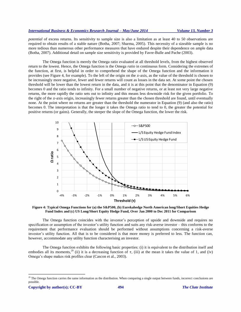
The Omega function is merely the Omega ratio evaluated at all threshold levels, from the highest observed
return to the lowest. Hence, the Omega function is the Omega ratio in continuous form. Considering the extremes of
the function, at first, is helpful in order to comprehend the shape of the Omega function and the information it
provides (see Figure 4, for example). To the left of the origin on the -axis, as the value of the threshold is chosen to
be increasingly more negative, fewer and fewer returns will count as losses in the data set. At some point the chosen
threshold will be lower than the lowest return in the data, and it is at this point that the denominator in Equation (9)
becomes 0 and the ratio tends to infinity. For a small number of negative returns, or at least not very large negative
returns, the more rapidly the ratio sets out to infinity and this means less downside risk for the given portfolio. To
the right of the -axis origin, increasingly fewer returns greater than the chosen threshold are found, until eventually
none. At the point where no returns are greater than the threshold the numerator in Equation (9) (and also the ratio)
becomes 0. The interpretation is that the longer it takes the Omega ratio to tend to 0, the greater the potential for
positive returns (or gains). Generally, the steeper the slope of the Omega function, the lower the risk.
Figure 4: Typical Omega Functions for (a) the S&P500, (b) Eurekahedge North American long/Short Equities Hedge
Fund Index and (c) US Long/Short Equity Hedge Fund, Over Jan 2000 to Dec 2011 for Comparison
The Omega function coincides with the investor’s perception of upside and downside and requires no
specification or assumption of the investor’s utility function and suits any risk-averse investor – this conforms to the
requirement that performance evaluation should be performed without assumptions concerning a risk-averse
investor’s utility function. All that is to be considered is that more money is preferred to less. The function can,
however, accommodate any utility function characterising an investor.
The Omega function exhibits the following basic properties: (i) it is equivalent to the distribution itself and
embodies all its moments,29
(ii) it is a decreasing function of , (iii) at the mean it takes the value of 1, and (iv)
Omega’s shape makes risk profiles clear (Cascon et al., 2003).
29 The Omega function carries the same information as the distribution. When comparing a single output between funds, incorrect conclusions are possible.
0
1
2
3
4
5
6
7
8
9
10
-4% -3% -2% -1% 0% 1% 2% 3% 4% 5% 6%
Ωra
tio
Threshold (τ)
S&P500
L/S Equity Hedge Fund Index
L/S US Equity Hedge Fund

International Business & Economics Research Journal – May/June 2014 Volume 13, Number 3
Copyright by author(s); CC-BY 495 The Clute Institute
The application of Omega as a measure of performance is particularly appropriate for non-normal return
distributions30
(Favre-Bulle & Pache, 2003) while Keating and Shadwick (2002) point out that the Omega may be
functional across a wide range of financial analysis and a range of hedge fund styles or strategies. Furthermore,
unlike the Sharpe and Sortino ratios, the Omega ratio discounts multimodal distributions. Estimation error risk can
also be reduced, as Omega is computed directly from the return distribution and measures the combined impact of
all moments instead of each one individually (Favre-Bulle & Pache, 2003). Favre-Bulle and Pache (2003) also argue
that within portfolio construction, the Omega offers a superior definition of risk and reward and as a consequence
may outperform optimisation performed with less precise measures.
Numerous studies have grouped funds by style and ranked them using different measures, and irrespective
of the measure used the ranking tend to be very similar (e.g., Nguyen-Thi-Thanh, 2010; Laing, 1999). It has been
shown that Omega has a low correlation with the Sharpe ratio and a reasonable assumption is therefore that Omega
rankings are not highly correlated with those of other traditional ratios. This is attributed to the additional higher
moment information that Omega captures and traditional mean-variance analysis does not (MoneyMate, 2009).
However, when returns are normally distributed or when higher moments are insignificant, Omega tends to agree
with traditional measures (Keating & Shadwick, 2002).
Omega based rankings are also always possible, irrespective of the threshold – unlike the Sharpe ratio
where ranking of negative-earning funds is inaccurate (de Wet, 2006). De Wet (2006) found that Omega also tends
to produce different results from other higher-moment measures, accenting that moments of order five and higher
should and do have an impact on performance measurement. It is not possible to determine precisely which
moments have the most influence as Omega measures the total influence of all the moments (Favre-Bulle & Pache,
2003).
Omega Metrics, although not the focus of this study, is another interesting development on the Omega
front. Omega Metrics is a natural generalisation of the Sharpe ratio and rewards a distribution for the size of its
mean and for the degree of concentration around the mean. In contrast to mean-variance measures, Omega Metrics
considers asymmetry and accounts explicitly for fat tails thus making it well-suited to hedge funds. Despite these
advantages, Omega Metrics has not, however, enjoyed substantial acceptance since its development (Shadwick,
2004; Keating, 2004).
3.2 Omega Modifications and Combinations
With growing acceptance of the Omega ratio by both practitioners and academics, modified versions of the
Omega ratio have proliferated.
Kazemi et al. (2003) introduced the Sharpe-Omega: a variation of Omega that maintains all of its desirable
features, provides the same information as Omega and always ranks investments the same as Omega. The
contribution of this measure is that it provides a measure of risk that is more intuitive than Omega and that is also
more similar to the Sharpe ratio. Kazemi et al. (2003) showed that Omega can be written as:
(10)
where is the price of a European call option written on the investment and is essentially the price of a
written European put option.31
The Sharpe-Omega of an investment is given by (Kazemi et al., 2003):
(11)
30 Because the Omega function incorporates all moments of a distribution. However, even for normally distributed returns, Omega provides addi-
tional information as it considers the investor’s preferences (for gains and losses) (Favre-Bulle & Pache, 2003). 31 Kazemi et al. (2003) asserted that the Omega’s numerator represents the “cost” of acquiring the return above a threshold and the denominator the “cost” of protecting a return below the threshold.
International Business & Economics Research Journal – May/June 2014 Volume 13, Number 3
Copyright by author(s); CC-BY 496 The Clute Institute
The Excess Omega Return, developed by Sortino et al. (1997), is the excess return actually earned on a
risk-adjusted basis. It portrays the variation between the Omega return of the investment portfolio and the Omega
return of the style benchmark. The geometric realised return(s), the style beta, the style downside variance and an
indicator of risk-aversion are included in the calculation.
Varadi (2012) proposed G-Omega, a simple Omega modification that attends to three failings of the
Omega, namely: (i) it is skewed by outliers,32
(ii) the sum measurement fails to account for the proper ratio of upside
versus downside return potential in the absence of a difference in frequency between the two, and (iii) it fails to
account for the impact of compounding returns.33
Quintessentially, the G-Omega is solely focused on the
compounding upside versus compounding downside potential, as it uses the geometric average returns above and
below the threshold.
MoneyMate Fund Ratings’ rating methodology combines the Omega ratio with another measure, downside
deviation, to produce innovative risk-adjusted performance fund ratings. Downside deviation is chosen as the
“combination” measure so as to additionally penalise downside risk34
as well as to differentiate among no-gain
funds.35
Downside deviation also aids in offsetting unintuitive results that may come about by Omega being
sensitive to the potential for excess returns. The methodology estimates standard deviation over the preceding 36
months using weekly total returns, whereafter the weekly standard deviation is annualised to correspond to volatility
over a single year (MoneyMate, 2009).
3.3 Data
The 26,496 monthly returns, net of management, and performance fees, from 184 ‘live’ individual36
hedge
funds sourced from a Eurekahedge database data extract between January 2000 and December 2011 were used for
this study. Funds with an incomplete monthly return history for the selected period were disregarded. Seeing that
hedge funds universally report performance figures on a monthly basis and also as it is compatible with investors’
month-end, holding-period return, monthly returns were chosen. Also, the data do not suffer from biases in the form
of survivorship, backfilling, or sampling while selection bias cannot be addressed as this would necessitate access to
returns from hedge funds that decide not to report.
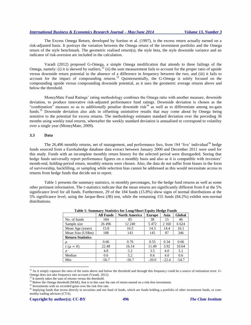
Table 1 presents the summary statistics, in monthly percentages, for the hedge fund returns as well as some
other pertinent information. The -statistics indicate that the mean returns are significantly different from 0 at the 5%
significance level for all funds. Furthermore, 29 of the 184 funds (15.8%) show signs of normal distributions at the
5% significance level, using the Jarque-Bera (JB) test, while the remaining 155 funds (84.2%) exhibit non-normal
distributions.
Table 1: Summary Statistics for Long/Short Equity Hedge Funds
All Funds North America Europe Asia Global
No. of funds 184 85 38 15 46
Sample size 26 496 12 240 5 472 2 160 6 624
Mean Age (years) 15.8 16.5 14.3 14.4 16.1
Mean Size (US$m) 188 143 145 87 346
Return Statistics
0.66 0.76 0.55 0.34 0.66
22.48 16.14 11.49 3.92 10.64
4.8 5.2 3.5 4.0 5.1
Median 0.6 5.2 0.6 4.0 0.6
Min -56.7 -56.7 -20.0 -22.4 -54.7
32 As it simply captures the ratio of the sums above and below the threshold and through this frequency could be a source of estimation error. G-
Omega does not take frequency into account (Varadi, 2012). 33 It merely takes the sum of returns versus the threshold. 34 Below the Omega threshold (MAR), that is in this case the rate of return earned on a risk-free investment. 35 Investments with no recorded gains over the risk-free rate. 36 Implying funds that invest directly in securities and not fund of funds, which are funds holding a portfolio of other investment funds, or com-modity trading advisors (CTA).
International Business & Economics Research Journal – May/June 2014 Volume 13, Number 3
Copyright by author(s); CC-BY 497 The Clute Institute
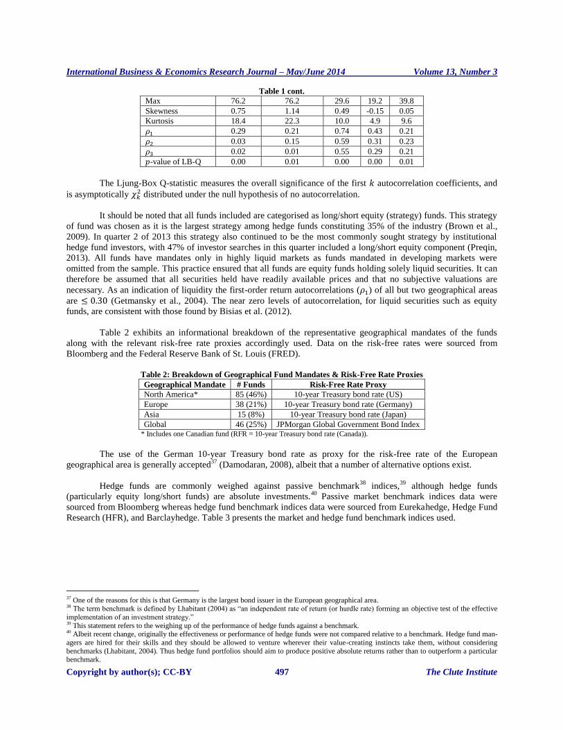
Table 1 cont.
Max 76.2 76.2 29.6 19.2 39.8
Skewness 0.75 1.14 0.49 -0.15 0.05
Kurtosis 18.4 22.3 10.0 4.9 9.6
0.29 0.21 0.74 0.43 0.21
0.03 0.15 0.59 0.31 0.23
0.02 0.01 0.55 0.29 0.21
-value of LB-Q 0.00 0.01 0.00 0.00 0.01
The Ljung-Box Q-statistic measures the overall significance of the first autocorrelation coefficients, and
is asymptotically distributed under the null hypothesis of no autocorrelation.
It should be noted that all funds included are categorised as long/short equity (strategy) funds. This strategy
of fund was chosen as it is the largest strategy among hedge funds constituting 35% of the industry (Brown et al.,
2009). In quarter 2 of 2013 this strategy also continued to be the most commonly sought strategy by institutional
hedge fund investors, with 47% of investor searches in this quarter included a long/short equity component (Preqin,
2013). All funds have mandates only in highly liquid markets as funds mandated in developing markets were
omitted from the sample. This practice ensured that all funds are equity funds holding solely liquid securities. It can
therefore be assumed that all securities held have readily available prices and that no subjective valuations are
necessary. As an indication of liquidity the first-order return autocorrelations ( ) of all but two geographical areas
are (Getmansky et al., 2004). The near zero levels of autocorrelation, for liquid securities such as equity
funds, are consistent with those found by Bisias et al. (2012).
Table 2 exhibits an informational breakdown of the representative geographical mandates of the funds
along with the relevant risk-free rate proxies accordingly used. Data on the risk-free rates were sourced from
Bloomberg and the Federal Reserve Bank of St. Louis (FRED).
Table 2: Breakdown of Geographical Fund Mandates & Risk-Free Rate Proxies
Geographical Mandate # Funds Risk-Free Rate Proxy
North America* 85 (46%) 10-year Treasury bond rate (US)
Europe 38 (21%) 10-year Treasury bond rate (Germany)
Asia 15 (8%) 10-year Treasury bond rate (Japan)
Global 46 (25%) JPMorgan Global Government Bond Index * Includes one Canadian fund (RFR = 10-year Treasury bond rate (Canada)).
The use of the German 10-year Treasury bond rate as proxy for the risk-free rate of the European
geographical area is generally accepted37
(Damodaran, 2008), albeit that a number of alternative options exist.
Hedge funds are commonly weighed against passive benchmark38
indices,39
although hedge funds
(particularly equity long/short funds) are absolute investments.40
Passive market benchmark indices data were
sourced from Bloomberg whereas hedge fund benchmark indices data were sourced from Eurekahedge, Hedge Fund
Research (HFR), and Barclayhedge. Table 3 presents the market and hedge fund benchmark indices used.
37 One of the reasons for this is that Germany is the largest bond issuer in the European geographical area. 38 The term benchmark is defined by Lhabitant (2004) as “an independent rate of return (or hurdle rate) forming an objective test of the effective
implementation of an investment strategy.” 39 This statement refers to the weighing up of the performance of hedge funds against a benchmark. 40 Albeit recent change, originally the effectiveness or performance of hedge funds were not compared relative to a benchmark. Hedge fund man-
agers are hired for their skills and they should be allowed to venture wherever their value-creating instincts take them, without considering
benchmarks (Lhabitant, 2004). Thus hedge fund portfolios should aim to produce positive absolute returns rather than to outperform a particular benchmark.
International Business & Economics Research Journal – May/June 2014 Volume 13, Number 3
Copyright by author(s); CC-BY 498 The Clute Institute
Table 3: Market and Hedge Fund Benchmark Indices
Benchmark Market Indices Region Specific
S&P500, S&P TSX* North America
DAX Europe
Nikkei 225 Asia
MSCI World Index Global
Benchmark Hedge Fund Indices Region Specific Style Specific
Eurekahedge North America Long/short Equities Index North America Long/short Equity
*The S&P TSX was included as one North American fund was a Canadian fund.
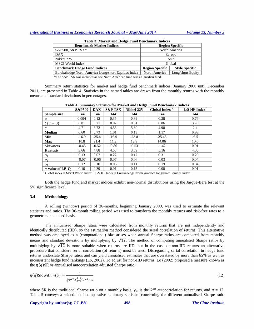
Summary return statistics for market and hedge fund benchmark indices, January 2000 until December
2011, are presented in Table 4. Statistics in the named tables are drawn from the monthly returns with the monthly
means and standard deviations in percentages.
Table 4: Summary Statistics for Market and Hedge Fund Benchmark Indices
S&P500 DAX S&P TSX Nikkei 225 Global Index + L/S HF Index*
Sample size 144 144 144 144 144 144
0.004 0.12 0.35 0.39 0.28 0.76
0.01 0.21 0.92 0.81 0.06 3.78
4.71 6.72 4.55 5.80 4.90 2.4
Median 0.60 0.73 1.01 0.13 1.17 0.99
Min -16.9 -25.4 -16.9 -23.8 -25.48 -6.5
Max 10.8 21.4 11.2 12.9 14.06 10.6
Skewness -0.43 -0.52 -0.86 -0.53 -1.42 0.01
Kurtosis 3.66 4.88 4.58 3.89 5.16 4.86
0.13 0.07 0.22 0.12 0.31 0.20
-0.07 -0.06 0.07 0.06 0.03 0.04
0.12 0.10 0.06 0.11 0.19 0.04
-value of LB-Q 0.10 0.39 0.01 0.15 0.00 0.01 + Global index = MSCI World Index. * L/S HF Index = Eurekahedge North America long/short Equities Index.
Both the hedge fund and market indices exhibit non-normal distributions using the Jarque-Bera test at the
5% significance level.
3.4 Methodology
A rolling (window) period of 36-months, beginning January 2000, was used to estimate the relevant
statistics and ratios. The 36-month rolling period was used to transform the monthly returns and risk-free rates to a
geometric annualised basis.
The annualised Sharpe ratios were calculated from monthly returns that are not independently and
identically distributed (IID), so the estimation method considered the serial correlation of returns. This alternative
method was employed as a (computational) bias arises when annual Sharpe ratios are computed from monthly
means and standard deviations by multiplying by . The method of computing annualised Sharpe ratios by
multiplying by is more suitable when returns are IID, but in the case of non-IID returns an alternative
procedure that considers serial correlation (of returns) must be used. Disregarding serial correlation in hedge fund
returns understate Sharpe ratios and can yield annualised estimates that are overstated by more than 65% as well as
inconsistent hedge fund rankings (Lo, 2002). To adjust for non-IID returns, Lo (2002) proposed a measure known as
the or annualised autocorrelation adjusted Sharpe ratio:
(12)
where SR is the traditional Sharpe ratio on a monthly basis, is the autocorrelation for returns, and = 12.
Table 5 conveys a selection of comparative summary statistics concerning the different annualised Sharpe ratio
International Business & Economics Research Journal – May/June 2014 Volume 13, Number 3
Copyright by author(s); CC-BY 499 The Clute Institute
computation methods based on the 184 long/short equity hedge funds. The summary statistics in Table 5 are based
on annualised geometric returns over a 36-month rolling period to facilitate presenting a statistical comparison
between the Sharpe ratio computation methods.
Table 5: Comparative Sharpe Ratio Summary Statistics (Annualised Figures)
Sharpe Ratio SC-adjusted Sharpe Ratio
Sample size 20 056* 20 056
0.38 0.41
0.85 0.95
Median 0.26 0.25
Min -2.1 -3.8
Max 3.5 5.1
Skewness 0.49 0.73
Kurtosis 2.86 3.92
*184 funds 109 (144-35) monthly returns.
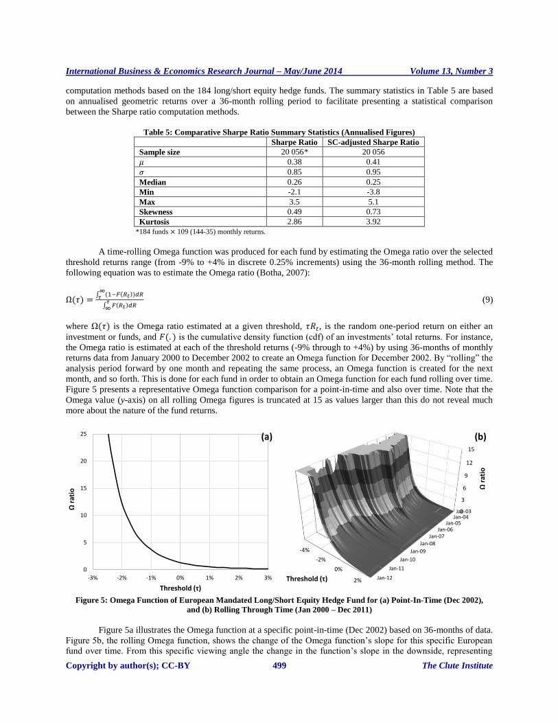
A time-rolling Omega function was produced for each fund by estimating the Omega ratio over the selected
threshold returns range (from -9% to +4% in discrete 0.25% increments) using the 36-month rolling method. The
following equation was to estimate the Omega ratio (Botha, 2007):
(9)
where is the Omega ratio estimated at a given threshold, , is the random one-period return on either an
investment or funds, and is the cumulative density function (cdf) of an investments’ total returns. For instance,
the Omega ratio is estimated at each of the threshold returns (-9% through to +4%) by using 36-months of monthly
returns data from January 2000 to December 2002 to create an Omega function for December 2002. By “rolling” the
analysis period forward by one month and repeating the same process, an Omega function is created for the next
month, and so forth. This is done for each fund in order to obtain an Omega function for each fund rolling over time.
Figure 5 presents a representative Omega function comparison for a point-in-time and also over time. Note that the
Omega value (y-axis) on all rolling Omega figures is truncated at 15 as values larger than this do not reveal much
more about the nature of the fund returns.
Figure 5: Omega Function of European Mandated Long/Short Equity Hedge Fund for (a) Point-In-Time (Dec 2002),
and (b) Rolling Through Time (Jan 2000 – Dec 2011)
Figure 5a illustrates the Omega function at a specific point-in-time (Dec 2002) based on 36-months of data.
Figure 5b, the rolling Omega function, shows the change of the Omega function’s slope for this specific European
fund over time. From this specific viewing angle the change in the function’s slope in the downside, representing
0
5
10
15
20
25
-3% -2% -1% 0% 1% 2% 3%
Ωra
tio
Threshold (τ)
(a)
-4%
-2%
0%
2%
0
3
6
9
12
15
Jan-03Jan-04
Jan-05Jan-06
Jan-07
Jan-08
Jan-09
Jan-10
Jan-11
Jan-12Threshold (τ)
Ωra
tio
(b)

International Business & Economics Research Journal – May/June 2014 Volume 13, Number 3
Copyright by author(s); CC-BY 500 The Clute Institute
risk, can be clearly seen as time passes. Figure 5b thus conveys additional information and perspective to an investor
compared to Figure 5a.
The subsequent section presents analysis and results by discussing how the rolling Omega function adds a
supplementary perspective for investors compared to the point-in-time Omega function. The section will also delve
into comparative fund rankings between the Sharpe and Omega ratios over time.
4. ANALYSIS AND RESULTS
4.1 The Visual Value of a Rolling Omega Function
The rolling Omega function has the added advantage of providing a supplementary perspective compared
to the point-in-time Omega function. This is so as a hedge fund investor can visually see and compare the
characteristics of a given fund with another fund or benchmark. Generally investors will use the relevant information
to construct a fund’s Sharpe and Omega ratios, which when graphed looks similar to Figure 6. Figure 6 presents the
rolling Sharpe and point-in-time Omega function’s of a randomly selected US long/short equity hedge fund (fund
#167) as well as an appropriate benchmark for this specific fund, the S&P500.
Figure 6: (a) Rolling Sharpe Ratio for a US Long/Short Equity Hedge Fund along with that of the S&P500 for Dec 2002
until Dec 2011, and (b) Point-In-Time (Dec 2002 and Dec 2011) Omega Functions for US Long/Short
Equity Hedge Fund and S&P500.
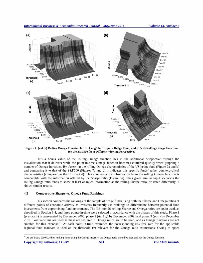
Figure 7 shows the rolling Omega function again for the same randomly selected US long/short equity
hedge fund (fund #167) as well as that of the S&P500 from two viewing perspectives. Figure 7 presents these rolling
Omega functions from two viewing angles to draw attention to the fact that the viewing perspective can be
customised to highlight specific characteristics.
-2
-1
0
1
2
3
4
Jan-02 Jan-04 Jan-06 Jan-08 Jan-10 Jan-12
Shar
pe
rati
o
S&P500
US L/S Equity Hedge Fund(a)
0
3
6
9
12
15
-6% -5% -4% -3% -2% -1% 0% 1% 2% 3%
Ωra
tio
Threshold (τ)
US Hedge Fund Dec '02
US Hedge Fund Dec '11
S&P500 Dec '02
S&P500 Dec '11
(b)
International Business & Economics Research Journal – May/June 2014 Volume 13, Number 3
Copyright by author(s); CC-BY 501 The Clute Institute
Figure 7: (a & b) Rolling Omega Function for US Long/Short Equity Hedge Fund, and (c & d) Rolling Omega Function
for the S&P500 from Different Viewing Perspectives
Thus a bonus value of the rolling Omega function lies in the additional perspective through the
visualisation that it delivers while the point-in-time Omega function becomes cluttered quickly when graphing a
number of Omega functions. By observing the rolling Omega characteristics of the US hedge fund (Figure 7a and b)
and comparing it to that of the S&P500 (Figures 7c and d) it indicates this specific funds’ rather countercyclical
characteristics (compared to the US market). This countercyclical observation from the rolling Omega function is
comparable with the information offered by the Sharpe ratio (Figure 6a). Thus given similar input scenarios the
rolling Omega ratio tends to show at least as much information as the rolling Sharpe ratio, or stated differently, it
shows similar results.
4.2 Comparative Sharpe vs. Omega Fund Rankings
This section compares the rankings of the sample of hedge funds using both the Sharpe and Omega ratios at
different points of economic activity as investors frequently use rankings to differentiate between potential fund
investments from unpromising fund investments. The (36-month) rolling Sharpe and Omega ratios are again used, as
described in Section 3.4, and three points-in-time were selected in accordance with the phases of this study. Phase 1
(pre-crisis) is represented by December 2006, phase 2 (during) by December 2009, and phase 3 (post) by December
2011. Points-in-time are used as these are required if Omega ratios are to be used, and as Omega functions are not
suitable for this exercise.41
At each point-in-time examined the corresponding risk-free rate for the applicable
regional fund mandate is used as the threshold ( ) relevant for the Omega ratio estimations. Owing to space
41 As per Botha (2007), when ranking funds using the Omega measure, the Omega ratio should be used and not the Omega function.
-9.00%-7.00%
-5.00%-3.00%
-1.00%1.00%
3.00%
Dec-02Dec-04
Dec-06Dec-08
Dec-10
Threshold (τ)
Ωra
tio
(a)
-9.00%-7.00%
-5.00%-3.00%
-1.00%1.00%
3.00%
Dec-02
Dec-03
Dec-04
Dec-05
Dec-06
Dec-07
Dec-08
Dec-09
Dec-10
Dec-11Threshold (τ)
Ωra
tio
(b)
-9.00%-7.00%
-5.00%-3.00%
-1.00%1.00%
3.00%
Dec-02Dec-04
Dec-06Dec-08
Dec-10
Threshold (τ)
Ωra
tio
(c)
-9.00%
-7.00%
-5.00%
-3.00%
-1.00%
1.00%
3.00%
Dec-02
Dec-04
Dec-06
Dec-08
Dec-10
Threshold (τ)
Ωra
tio
(d)

International Business & Economics Research Journal – May/June 2014 Volume 13, Number 3
Copyright by author(s); CC-BY 502 The Clute Institute
constraints the top and bottom 20 funds in the sample are identified at December 2009 according to the Sharpe ratio,
and then ranked backwards and forwards in time within the full fund data sample of 184 funds. Hereafter the Omega
ratios are calculated at the relevant points-in-time, the funds ranked and then the fund rankings of the Sharpe and
Omega compared.
Figure 8: Sharpe Ratio vs. Omega Ratio Values for the Top and Bottom 20 Funds in the Sample for (a) Phase 1, (b) Phase
2, and (c) Phase 3. Sharpe Ratio vs. Omega Ratio Rank for the Top and Bottom 20 funds in the Sample for
(d) Phase 1, (e) Phase 2, and (f) Phase 3
Figure 8 presents comparative Sharpe and Omega values as well as rankings for the top and bottom 20
funds for the three economic phases. Figure 8 clearly indicates the noticeable shift in fund performance during the
crisis as opposed to prior, as a visible distinction is evident between strong and weak performing funds. Also evident
from Figure 8b (representing the phase during the crisis) is that a large contingent of the top performing funds
cluster around a Sharpe ratio equal to 1 - just rewarding investors with a parallel amount of return for the amount of
risk taken on-board. Thus even the top performing funds did not deliver exceptional performance compared to
performance expectations during normal economic conditions. However, during this particular period this level of
performance would be classified as exceptional – and thus why these funds are the top funds during phase 2.
0
2
4
6
8
10
-1 0 1 2 3 4
Ωra
tio
Sharpe ratio
PHASE 1 Best performing (2009) Worst performing (2009)
(a)0
1
2
3
4
5
6
7
-2 -1 0 1 2 3
Ωra
tio
Sharpe ratio
PHASE 2 Best performing (2009) Worst performing (2009)
(b)
0
2
4
6
8
-2 -1 0 1 2 3
Ωra
tio
Sharpe ratio
PHASE 3 Best performing (2009) Worst performing (2009)
(c)
162, 155
167, 111101, 125
5, 99
3, 32
74, 37
65, 118
0
40
80
120
160
200
0 20 40 60 80 100 120 140 160 180 200
Om
ega
ran
k
Sharpe rank
PHASE 1 Best performing (2009) Worst performing (2009)
(d)
10
14, 58
20, 7
165, 50
172, 108
0
40
80
120
160
200
0 20 40 60 80 100 120 140 160 180 200
Om
ega
ran
k
Sharpe rank
PHASE 2 Best performing (2009) Worst performing (2009)
(e)
116, 69
37, 35
107, 170
52, 76
0
40
80
120
160
200
0 20 40 60 80 100 120 140 160 180 200
Om
ega
ran
k
Sharpe rank
PHASE 3 Best performing (2009) Worst performing (2009)
(f)

International Business & Economics Research Journal – May/June 2014 Volume 13, Number 3
Copyright by author(s); CC-BY 503 The Clute Institute
During the crisis period (Figure 8b and 8e) both good and bad performing funds were clearly identified and
valued accordingly by both the Sharpe and Omega ratios. The visual results from Figure 8 is also similar to those
found by Botha (2007) in that for low Sharpe and Omega ratios the ranking of the funds is alike. However, for
higher Sharpe ratios the ranking accuracy deteriorates to a degree – this is, however, interestingly less the case
during phase 2 which represents the period during the crisis.
It is moreover apparent that some of the top funds during the crisis performed badly prior to the crisis. This
suggests that investors would possibly not have selected these funds prior to the crisis due to mediocre or weak risk-
adjusted performance, and yet these funds performed the best during the crisis. As an example of this, see and
compare the positioning of the indicated fund (Fund #167 as the larger datum point) in Figures 8a, 8b, and 8c.
The comparative fund rankings based on the Sharpe and Omega ratios for phases 1 to 3 are presented in
Figures 8d, 8e, and 8f respectively. The numbers next to the filled points are the (Sharpe ratio, Omega ratio) rank
coordinates.
In the period prior to the financial crisis a wider discrepancy between the Sharpe and Omega ratio rankings
existed than compared to the period during the crisis, (this phenomenon is to some extent reinitiated in the post-
crisis phase). It is once again visibly clear, although now according to fund rankings, that there was a clear
distinction between the best and worst performing funds during the financial crisis period (Phase 2). During the
crisis period the Sharpe and Omega ratios also generally ranked the funds similarly, although there were a small
number of exceptions (see funds in southeast region of Figure 8e). The comparative rankings reiterates the point
made earlier that selecting a highly ranked fund prior to the crisis resulted in a weak rank for the same fund during
the crisis period – as some of the worst ranked funds during the crisis are ranked rather highly in the period prior to
the crisis. As an example of this phenomenon see and compare the ranking position of the indicated fund (fund #167
indicated by larger datum) in Figures 8d, 8e, and 8f.
Both Sharpe ratio and Omega ratio rankings agree well for lower rankings, although there is less agreement
between the rankings based on these measures for higher ranked funds – these higher ranked will be more closely
scrutinised by investors as they will generate the most investor interest. It is, however, interesting that during the
height of the 2007 economic crisis these two performance measures were in considerable (fund ranking) agreement
for both low and high ranked funds, compared to the economic periods both prior and after the crisis.
4.3 Selective Statistics over Different Economic Conditions
This section presents some selective summary performance statistics in the form of returns, Sharpe and
Omega ratios for both the hedge funds in this study and relevant benchmarks to these funds in market indices. This
highlights the changing characteristics of the funds and their market benchmarks throughout different economic
periods, as the statistics are partitioned into three phases. The three phases represent the periods prior, during, and
post the 2007 financial crisis. January 2002 until December 2006 constitutes Phase 1, January 2007 until December
2009 Phase 2, and January 2010 until December 2011 Phase 3. This section employs a rolling annual calculation
methodology based on 36-months, as discussed in Section 3.4.
The changing characteristics of all funds during the three phases are presented in Figure 9 through the
average Sharpe ratio as well as the average annual return and standard deviation for all funds employed in this study.
Table 6 presents the summary statistics for all funds per phase.

International Business & Economics Research Journal – May/June 2014 Volume 13, Number 3
Copyright by author(s); CC-BY 504 The Clute Institute
Figure 9: Average Annual Return and Standard Deviation and also Sharpe Ratio for All Hedge Funds
From Figure 9 the impact of the 2007 financial crisis can be seen through a decrease in the average Sharpe
ratio of all funds during Phase 2. Figure 9 also draws attention to the decrease in average returns across all funds
along with the almost simultaneous increase in volatility. Also, mostly during Phase 2 which presents the period
during the 2007 financial crisis, the average Sharpe ratio of all funds falls to below zero which implies that a risk-
less asset would have performed better on average during this time compared to the analysed funds sample. The
visual results in Figure 9 are echoed in the summary statistics as in Table 6, which shows similar declining average
returns and Sharpe ratios for all funds from Phase 1 through to Phase 3. The average Omega ratios also decreases
through time, while interestingly the standard deviation of the returns, Sharpe and Omega ratios reduce over time
indicating that the performance spectrum between funds on average diminishes.
Table 6: Summary Statistics for All Hedge Funds per Phase
Phase 1 Phase 2 Phase 3 Phase 1 Phase 2 Phase 3 Phase 1 Phase 2 Phase 3
Return Statistics Sharpe Ratio Statistics Omega Ratio Statistics
9016 6624 4416 9016 6624 4416 184 184 184
10.41% 6.86% 2.39% 0.63 0.43 -0.07 3.34 1.76 1.27
10.93% 10.20% 8.38% 1.03 0.92 0.54 4.39 2.22 0.88
Median 9.59% 7.33% 2.21% 0.54 0.31 -0.11 2.20 1.11 1.15
Min -44.96% -48.39% -36.57% -3.79 -1.95 -2.30 0.46 0.42 0.02
Max 59.50% 42.39% 74.37% 5.07 4.39 4.12 32.79 12.98 7.01
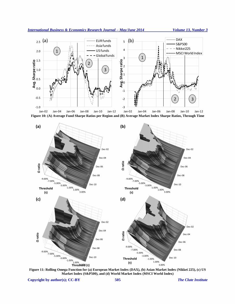
The average Sharpe ratios of both funds and their relevant market indices, per region, are presented in
Figure 10. From this figure, is it clear that funds and market indices from all the included regions behaved similarly
across the three phases. None of the regional funds or benchmarks indicate significantly better performance than any
other during or post the financial crisis. However, Asian funds performed better, on average, shortly prior to the
crisis but also performed the worst during the crisis period (Figure 10a).
-1.00
-0.50
0.00
0.50
1.00
1.50
2.00
-5%
0%
5%
10%
15%
20%
25%
Dec-02 Dec-03 Dec-04 Dec-05 Dec-06 Dec-07 Dec-08 Dec-09 Dec-10 Dec-11
Avg
. Sh
arp
e ra
tio
Avg
. An
nu
alis
ed %
Ret
urn
/ St
d D
ev
All funds return
All funds std dev
All funds Sharpe ratio
1 2 3
International Business & Economics Research Journal – May/June 2014 Volume 13, Number 3
Copyright by author(s); CC-BY 505 The Clute Institute
Figure 10: (A) Average Fund Sharpe Ratios per Region and (B) Average Market Index Sharpe Ratios, Through Time
Figure 11: Rolling Omega Function for (a) European Market Index (DAX), (b) Asian Market Index (Nikkei 225), (c) US
Market Index (S&P500), and (d) World Market Index (MSCI World Index)
-1.0
-0.5
0.0
0.5
1.0
1.5
2.0
2.5
Jan-02 Jan-04 Jan-06 Jan-08 Jan-10 Jan-12
Av
g. S
ha
rpe
ra
tio
EUR funds
Asia funds
US funds
Global funds
2
3
1
-3
-2
-1
0
1
2
3
4
5
Jan-02 Jan-04 Jan-06 Jan-08 Jan-10 Jan-12
Av
g. S
ha
rpe
ra
tio
DAXS&P500Nikkei225MSCI World Index
3
1
2
(b)(a)
-9.00%-7.00%
-5.00%-3.00%
-1.00%1.00%
3.00%
Dec-02
Dec-04
Dec-06
Dec-08
Dec-10
Ωra
tio
Threshold (τ)
(a)
-9.00%-7.00%
-5.00%-3.00%
-1.00%1.00%
3.00%
Dec-02
Dec-04
Dec-06
Dec-08
Dec-10
Ωra
tio
Threshold (τ)
(b)
-9.00%-7.00%
-5.00%-3.00%
-1.00%1.00%
3.00%
Dec-02
Dec-04
Dec-06
Dec-08
Dec-10
Threshold (τ)
Ωra
tio
(c)
-9.00%-7.00%
-5.00%-3.00%
-1.00%1.00%
3.00%
Dec-02
Dec-04
Dec-06
Dec-08
Dec-10Threshold (τ)
Ωra
tio
(d)
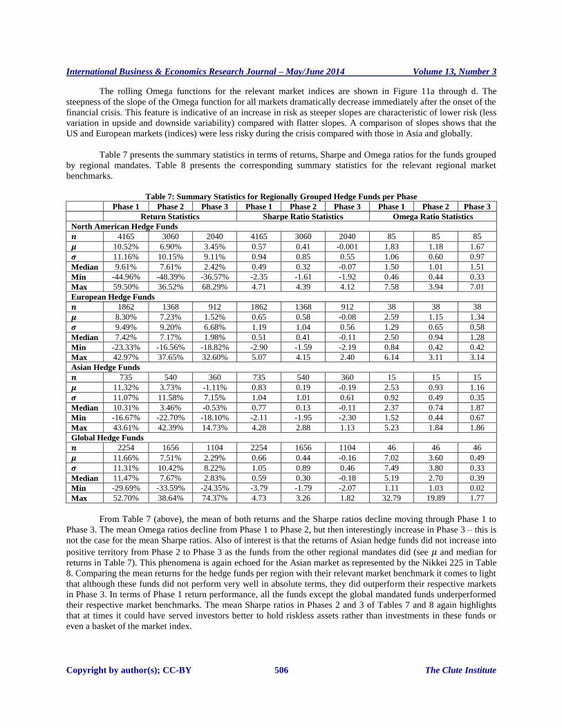
International Business & Economics Research Journal – May/June 2014 Volume 13, Number 3
Copyright by author(s); CC-BY 506 The Clute Institute
The rolling Omega functions for the relevant market indices are shown in Figure 11a through d. The
steepness of the slope of the Omega function for all markets dramatically decrease immediately after the onset of the
financial crisis. This feature is indicative of an increase in risk as steeper slopes are characteristic of lower risk (less
variation in upside and downside variability) compared with flatter slopes. A comparison of slopes shows that the
US and European markets (indices) were less risky during the crisis compared with those in Asia and globally.
Table 7 presents the summary statistics in terms of returns, Sharpe and Omega ratios for the funds grouped
by regional mandates. Table 8 presents the corresponding summary statistics for the relevant regional market
benchmarks.
Table 7: Summary Statistics for Regionally Grouped Hedge Funds per Phase
Phase 1 Phase 2 Phase 3 Phase 1 Phase 2 Phase 3 Phase 1 Phase 2 Phase 3
Return Statistics Sharpe Ratio Statistics Omega Ratio Statistics
North American Hedge Funds
4165 3060 2040 4165 3060 2040 85 85 85
10.52% 6.90% 3.45% 0.57 0.41 -0.001 1.83 1.18 1.67
11.16% 10.15% 9.11% 0.94 0.85 0.55 1.06 0.60 0.97
Median 9.61% 7.61% 2.42% 0.49 0.32 -0.07 1.50 1.01 1.51
Min -44.96% -48.39% -36.57% -2.35 -1.61 -1.92 0.46 0.44 0.33
Max 59.50% 36.52% 68.29% 4.71 4.39 4.12 7.58 3.94 7.01
European Hedge Funds
1862 1368 912 1862 1368 912 38 38 38
8.30% 7.23% 1.52% 0.65 0.58 -0.08 2.59 1.15 1.34
9.49% 9.20% 6.68% 1.19 1.04 0.56 1.29 0.65 0.58
Median 7.42% 7.17% 1.98% 0.51 0.41 -0.11 2.50 0.94 1.28
Min -23.33% -16.56% -18.82% -2.90 -1.59 -2.19 0.84 0.42 0.42
Max 42.97% 37.65% 32.60% 5.07 4.15 2.40 6.14 3.11 3.14
Asian Hedge Funds
735 540 360 735 540 360 15 15 15
11.32% 3.73% -1.11% 0.83 0.19 -0.19 2.53 0.93 1.16
11.07% 11.58% 7.15% 1.04 1.01 0.61 0.92 0.49 0.35
Median 10.31% 3.46% -0.53% 0.77 0.13 -0.11 2.37 0.74 1.87
Min -16.67% -22.70% -18.10% -2.11 -1.95 -2.30 1.52 0.44 0.67
Max 43.61% 42.39% 14.73% 4.28 2.88 1.13 5.23 1.84 1.86
Global Hedge Funds
2254 1656 1104 2254 1656 1104 46 46 46
11.66% 7.51% 2.29% 0.66 0.44 -0.16 7.02 3.60 0.49
11.31% 10.42% 8.22% 1.05 0.89 0.46 7.49 3.80 0.33
Median 11.47% 7.67% 2.83% 0.59 0.30 -0.18 5.19 2.70 0.39
Min -29.69% -33.59% -24.35% -3.79 -1.79 -2.07 1.11 1.03 0.02
Max 52.70% 38.64% 74.37% 4.73 3.26 1.82 32.79 19.89 1.77
From Table 7 (above), the mean of both returns and the Sharpe ratios decline moving through Phase 1 to
Phase 3. The mean Omega ratios decline from Phase 1 to Phase 2, but then interestingly increase in Phase 3 – this is
not the case for the mean Sharpe ratios. Also of interest is that the returns of Asian hedge funds did not increase into
positive territory from Phase 2 to Phase 3 as the funds from the other regional mandates did (see and median for
returns in Table 7). This phenomena is again echoed for the Asian market as represented by the Nikkei 225 in Table
8. Comparing the mean returns for the hedge funds per region with their relevant market benchmark it comes to light
that although these funds did not perform very well in absolute terms, they did outperform their respective markets
in Phase 3. In terms of Phase 1 return performance, all the funds except the global mandated funds underperformed
their respective market benchmarks. The mean Sharpe ratios in Phases 2 and 3 of Tables 7 and 8 again highlights
that at times it could have served investors better to hold riskless assets rather than investments in these funds or
even a basket of the market index.

International Business & Economics Research Journal – May/June 2014 Volume 13, Number 3
Copyright by author(s); CC-BY 507 The Clute Institute
Table 8: Summary Statistics for Market Indices per Phase.
Phase 1 Phase 2 Phase 3 Phase 1 Phase 2 Phase 3 Phase 1 Phase 2 Phase 3
Return Statistics Sharpe Ratio Statistics Omega Ratio Statistics
49 36 24 49 36 24 49 36 24
US Market Index – S&P500
-1.54% 9.14% -1.80% 0.0002 0.84 -0.18 1.11 1.09 1.69
19.17% 13.29% 5.63% 1.34 1.30 0.233 0.58 0.56 1.03
Median -6.02% 10.91% -3.62% -0.39 0.36 -0.26 0.93 0.95 1.27
Min -31.68% -12.80% -9.35% -2.41 -0.56 -0.46 0.41 0.35 0.53
Max 35.05% 26.51% 9.25% 2.64 3.12 0.32 2.41 2.08 4.02
European Market Index – DAX
0.86% 9.14% -1.80% -0.08 0.05 -0.23 1.32 1.90 0.98
9.75% 13.29% 5.63% 0.79 0.77 0.36 0.90 1.17 0.18
Median 1.82% 10.91% -3.62% -0.16 -0.20 -0.33 0.86 1.52 0.93
Min -17.28% -12.80% -9.35% -2.04 -0.82 -0.59 0.37 0.56 0.75
Max 15.14% 26.51% 9.25% 1.15 1.49 0.78 3.80 3.93 1.38
Asian Market Index – Nikkei 225
1.77% -1.07% -11.29% -0.09 0.06 -0.64 1.36 1.22 0.74
15.69% 14.41% 5.90% 1.13 0.77 0.29 0.84 0.71 0.15
Median 1.29% 3.18% -12.40% 0.002 -0.17 -0.72 1.05 1.14 0.73
Min -26.81% -22.41% -19.73% -2.98 -0.82 -1.07 0.37 0.37 0.56
Max 29.24% 17.25% 1.57% 1.43 1.49 0.03 3.43 2.33 1.10
Global Market Index – MSCI World
6.42% 4.95% -3.46% 0.29 0.52 -0.28 3.72 4.21 0.35
12.43% 12.88% 6.37% 1.56 1.04 0.26 3.18 3.18 0.06
Median 8.08% 10.02% -4.66% 0.17 0.38 -0.35 2.46 3.64 0.35
Min -13.36% -16.59% -11.89% -2.93 -0.69 -0.56 0.84 0.91 0.27
Max 27.41% 20.99% 12.29% 4.48 2.33 0.42 12.18 10.67 0.45
5. SUMMARY AND CONCLUSION
The Omega function was used to augment the Sharpe ratio as a performance measure in the hedge fund
context. ‘Live,’ individual, long/short, equity hedge funds, sourced from the Eurekahedge database and spanning
geographical mandates that included North America, Europe, Asia, and global were used, covering the period
January 2000 to December 2011. A Sharpe ratio annualisation method that considers the serial correlation of returns
was also used to correct for non-IID errors.
Results were presented in three sections. Firstly, using a 36-month rolling (window) analysis, Omega
functions were constructed by estimating the Omega ratio over a range of return thresholds over time. These may
assist investors, to (i) observe the change in the Omega function over time for either a fund or its applicable
benchmark and (ii) compare the change in the Omega function over time between funds. This additional perspective
thus provides investors with information as to how a fund performed during specific periods, for instance the 2007
financial crisis.
Secondly, comparative Sharpe versus Omega fund values and rankings were assembled using the 36-month
rolling method at different points of economic activity (pre-, during, and post crisis) to gauge how these measures
value and rank funds over changing economic conditions. The top and bottom 20 ranked funds in the data sample
were identified at a point during the crisis period according to the Sharpe ratio, and then ranked both backwards and
forwards in time within the full data sample. Noticeable shifts in fund performance during the 2007 crisis were
observed. A large contingent of top performing funds was also found to cluster around a Sharpe ratio of 1 during this
period. A clear distinction is evident between the best and worst performing funds during the crisis period. In
comparison the periods prior and post the financial crisis sees a wider discrepancy between the Sharpe and Omega
ratio rankings. The fund rankings are alike for funds with low Sharpe and Omega ratios a result similar to that found
by Botha (2007) while for higher Sharpe ratios the ranking accuracy deteriorates somewhat – less so in the case
during the crisis period. Moreover it is found that some of the top funds during the crisis performed poorly prior to

International Business & Economics Research Journal – May/June 2014 Volume 13, Number 3
Copyright by author(s); CC-BY 508 The Clute Institute
the crisis suggesting that investors would possibly not have selected these funds prior to the crisis due their mediocre
or weak risk-adjusted performance. Most interesting is the fact that during the crisis period these two performance
were in considerable agreement in terms of fund ranking for both low and high ranked funds, compared to the
economic period both prior and after the crisis.
Thirdly, to highlight the changing characteristics of hedge funds and their respective market benchmarks
over the varying economic conditions around the 2007 financial crisis, a selective statistical analysis of returns was
conducted. Results indicate a decrease in the average return as well as a simultaneous increase in volatility across all
funds during the crisis period with average Sharpe ratios often falling below zero. Mean Omega ratios increase after
the crisis while mean Sharpe ratios do not. Geographically, it was found that funds and market indices from all
included regions behave similarly across the three phases and none of the regional funds or benchmarks indicate
significantly better performance than another during or post the financial crisis. In the period prior to the crisis Asian
funds performed better, on average. For market indices, an immediate increase in risk after the onset of the financial
crisis was observed: North American and European markets (indices) were less risky during the crisis period
compared to those in Asia and globally. Hedge funds from all regions outperformed their relevant market indices
prior to the crisis.
The need to accurately distinguish between poor and good quality fund returns has not diminished, and in
actual fact is ever increasing. Higher moments of the return distributions must be accounted for if accurate fund
comparisons (in terms of risk-adjusted returns or fund rankings) are desired.
The Omega function, though not a perfect measure, presents an arguably substantial enhancement
compared with traditional performance measures as it describes a large extent of the underlying distribution
structure, which is highly relevant and significant to hedge funds. The rolling Omega function also demonstrates its
added value as investors can gauge the risk and return characteristics of specific investments, through time, by
customising viewing perspectives.
Considerations for future research should, however, be aimed at a method that uses the Omega function
when ranking funds as the Omega function considers the full distribution and not just a single return threshold as is
the case with the Omega ratio that is currently being used to rank funds.
ACKNOWLEDGEMENTS
This work is based on research financially supported by the National Research Foundation (NRF) along with the
University of South Africa. Any opinion, finding and conclusion or recommendation expressed in this material is
that of the author(s): the NRF and the University of South Africa do not accept any liability in this regard.
The Workwell Research Unit at the North-West University, Potchefstroom, South Africa, for their financial
assistance in procuring the data.
The authors would like to express their gratitude to the scientific committee of the Biennial Conference of the
Economic Society of South Africa for the opportunity to deliver this paper at the conference on the 25th
of
September 2013 held at the University of the Free State, Bloemfontein, South Africa.
AUTHOR INFORMATION
Francois van Dyk began his career in South Africa as a risk analyst specialising in Basel II at FirstRand Bank Ltd.
He furthered his career as a senior consultant at a niche international risk consultancy. He currently holds a senior
lecturing position at the University of South Africa. This study forms part of his PhD in risk management at the
North-West University (Potchefstroom campus) which focuses on novel, quantitative risk measures within a hedge
fund context. He obtained his Masters in risk, focusing on investment portfolio risk, cum laude. He holds a PRM and
CHP and is currently pursuing his CFA qualification. Senior lecturer in the Department of Finance, Risk
Management and Banking, UNISA, Pretoria, South Africa. E-mail: [email protected] (Corresponding author)

International Business & Economics Research Journal – May/June 2014 Volume 13, Number 3
Copyright by author(s); CC-BY 509 The Clute Institute
Gary van Vuuren, Ph.D., began his career with a Masters in astrophysics and a PhD in nuclear physics. He
transferred to quantitative finance and, after a spell at Goldman Sachs in London, obtained a Masters in market risk
and a PhD in credit risk. He then worked as a risk manager for South African retail banks and asset managers before
moving to London and working in retail and investment banks. He settled on quantitative risk assessment and
management in financial institutions for Fitch Ratings where he remains employed. He is an accredited GARP
Financial Risk Manager. Extraordinary professor at the School of Economics, North-West University,
Potchefstroom Campus, South Africa. E-mail: [email protected]
André Heymans, Ph.D. After completing his PhD in finance in 2007, André Heymans moved to London where he
was employed by BNY MELLON until the middle of 2008. He then moved to South Africa to fill the position of
Head: Research and Development in the trading room at an agricultural trading firm (Free State Maize). André
moved back to academia in April 2009 where he currently holds the position Program Head of Risk Management.
Programme leader in Risk Management at the School of Economics, North-West University, Potchefstroom, South
Africa. E-mail: [email protected]
REFERENCES
1. Ackermann, C., Mcenally, R., & Ravenscraft, D. (1999). The performance of hedge funds: Risk, returns
and Incentives. Journal of Finance, 54(3), 833-874.
2. Agarwal, V., & Naik, N. Y. (2004). Risk and portfolio decisions involving hedge funds. Review of
Financial Studies, 17(1), 63-98.
3. Agarwal, V., Daniel, N. D., & Naik, N. Y. (2011). Do hedge funds manage their reported returns? The
Review of Financial Studies, 24(10), 3281-3320.
4. Amin, G. S., & Kat, H. M. (2001). Hedge fund performance 1990-2000 – Do the ‘money machines’ really
add value? (ICMA Centre working paper). SSRN. Retrieved 5 Jan. 2013 from
http://papers.ssrn.com/sol3/papers.cfm?abstract_id=270074
5. Artzner, P., Delbaen, F., Eber, J. M., & Heath, D. (1997). Thinking coherently. Risk Magazine, 10(11), 68-
71.
6. Barclayhedge (2013). Retrieved 29 June 2013 from
http://www.barclayhedge.com/research/indices/ghs/mum/Hedge_Fund.html
7. Bernardo, A. E., & Ledoit, O. (2000). Gain, loss and asset pricing. Journal of Political Economy, 108(1),
144-172.
8. Bisias, D., Flood, M., Lo, A. W., & Valavanis, S. (2012). A survey of systemic risk analytics. Annual
Review of Financial Economics, 4(1), 255-296.
9. Botha, M. (2007). A comparison of South African hedge fund risk measures. South African Journal of
Economics, 75(3), 459-477.
10. Boyd, J. (2013). Hedge funds up 6.19% in 2012 – Eurekahedge. Investment Europe. 22 January. Retrieved
23 July 2013 from http://www.investmenteurope.net/investment-europe/news/2238090/hedge-funds-up-
619-in-2012eurekahedge
11. Brooks, C., & Kat, H. M. (2002). The statistical properties of hedge fund index returns and their
implications for investors. Journal of Alternative Investments, 5(2), 26-44.
12. Brown, S. J, Kacperczyk, M., Ljungqvist, A., Lynch, A., Pedersen, L., & Richardson, M. (2009). Hedge
funds in the aftermath of the financial crisis. Financial Markets, Institutions & Instruments, 18(2), 155-156.
13. Cascon, A., Keating, C., & Shadwick, W. F. (2003). The Omega function. Finance Development Centre.
Retrieved 6 July 2013 from http://www.performancemeasurement.org/CasconKeatingShadwick2003.pdf
14. Chan, N., Getmansky, M., Haas, S. M., & Lo, A. W. (2005). Systemic risk and hedge funds. Optimization,
920(617), 235-338.
15. Clarke, W. (2012). Hedge fund launches still below their pre-crisis peak. Investment Europe. 15 March.
Retrieved 3 March 2013 from http://www.investmenteurope.net/investment-europe/news/2159709/hedge-
fund-launches-pre-crisis-peak
16. Damodaran, A. (2008). What is the riskfree rate? A search for the basic building block. (Working paper).
SSRN. Retrieved 15 March 2013 from http://papers.ssrn.com/sol3/papers.cfm?abstract_id=1317436
17. De Wet, R. (2006). The evaluation of Omega as an effective tool for portfolio evaluation in the South
African context. (Research report - MBA). Stellenbosch: University of Stellenbosch.
International Business & Economics Research Journal – May/June 2014 Volume 13, Number 3
Copyright by author(s); CC-BY 510 The Clute Institute
18. Dowd, K. (2000). Adjusting for risk: An improved Sharpe ratio. International Review of Economics and
Finance, 9(3), 209-222.
19. Eling, M., & Schumacher, F. (2006). Hat die wahl des perfromancemaßes einen einfluss auf die
Beurteilung von hedgefondsindizes? Kredit and Kapital, 39(3), 419-457.
20. Eurekahedge. (2010). 2010 key trends in global hedge funds. Hedge Fund Monthly, August. Retrieved 23
Feb. 2013 from http://www.eurekahedge.com/news/10_aug_EH_Aug-10_GHF_Key_Trends_ABR.asp
21. Eurekahedge. (2012). 2012 key trends in global hedge funds. Hedge Fund Monthly, July. Retrieved 19 Feb.
2013 from http://www.eurekahedge.com/news/Eurekahedge_Jul_2012_Global_Hedge_
Funds_Key_Trends.asp
22. Eurekahedge. (2013a). The Eurekahedge report. June. Retrieved 19 June 2013 from
http://www.eurekahedge.com/news/13_jun_Eurekahedge_Report_online.asp
23. Eurekahedge. (2013b). 2013 key trends in global hedge funds. Retrieved 16 July 2013 from
http://www.eurekahedge.com/news/Eurekahedge_Jul_2013_Global_Hedge_Fund_Key_Trends.asp
24. Farinelli, S., & Tibiletti, L. (2008). Sharpe thinking in asset ranking with one-sided measures. European
Journal of Operational Research, 185(3), 1542-1547.
25. Favre-Bulle, A., & Pache, S. (2003). The Omega measure: Hedge fund optimization. (Working paper).
SSRN. Retrieved 15 Jan. 2013 from http://papers.ssrn.com/sol3/papers.cfm?abstract_id=365740
26. Feng, S. (2011). Three essays on hedge fund fee structure, return smoothing and gross performance.
(Dissertation – D.Phil). Amherst: University of Massachusetts.
27. Fung, W., & Hsieh, D. A. (1997). Empirical characteristics of dynamic trading strategies: The case of
hedge funds. Review of Financial Studies, 10(2), 275-302.
28. Fung, W., & Hsieh, D. A. (2001). The risk in hedge funds strategies: theory and evidence from trend
followers. Review of Financial Studies, 14(2), 313-341.
29. Getmansky, M., Lo, A., & Makarov, I. (2004). An econometric analysis of serial correlation and illiquidity
in hedge fund returns. Journal of Financial Economics, 74(3), 529-609.
30. Getmansky, M., Billio, M., Lo, A. W., & Pelizzon, L. (2012). Econometric measures of connectedness and
systemic risk in the finance and insurance sectors. Journal of Financial Economics, 104(3), 536-559.
31. Gibbons, M., Ross, S., & Shanken, J. (1989). A test of the efficiency of a given portfolio. Econometrica,
57(5), 1121-1152.
32. Goetzmann, W., Ingersoll, J., & Spiegel, M. (2007). Portfolio performance manipulation and manipulation-
proof performance measures. Review of Financial Studies, 20(5), 1503-1546.
33. Goetzmann, W., Ingersoll, J., Spiegel, M., & Welch, I. (2002). Sharpening Sharpe ratios. (Working paper).
NBER.
34. Gregoriou, G. N., & Geuyie, J. P. (2003). Risk-adjusted performance of funds of hedge funds using a
modified Sharpe ratio. Journal of Wealth Management, 6(3), 77-83.
35. Harlow, W. V. (1991). Asset allocation in a downside-risk framework. Financial Analysts Journal, 47(5),
28-40.
36. Hodges, S. (1998). A generalization of the Sharpe ratio and its applications to valuation bounds and risk
measures. (Working paper). Financial Options Research Centre. Retrieved 29 June 2013 from
http://www2.warwick.ac.uk/fac/soc/wbs/subjects/finance/research/wpaperseries/1998/98-88.pdf
37. Jobson, J. D., & Korkie, B. M. (1981). Performance hypothesis testing with the Sharpe and Treynor
measures. Journal of Finance, 36(4), 889-908.
38. Joenväärä, J., Kosowski, R., & Tolonen, P. (2012). Revisiting ‘stylized facts’ about hedge funds: Insights
from a novel aggregation of the main hedge fund databases. SSRN. Retrieved 3 Aug. 2013 from
http://ssrn.com/abstract=1989410
39. Kaiser, D., & Haberfelner, F. (2012). Hedge fund biases after the financial crisis. Managerial Finance,
38(1), 27-43.
40. Kaplan, P., & Knowles, J. (2004). Kappa: A generalised downside risk-adjusted performance measure.
Journal of Performance Measurement, 8(3), 42-54.
41. Kat, H. M., & Amin, G. S. (2001). Welcome to the dark side: Hedge fund attrition and survivorship bias
over the period 1994-2001. (Working paper). SSRN Retrieved 1 March 2013 from
http://papers.ssrn.com/sol3/papers.cfm?abstract_id=293828

International Business & Economics Research Journal – May/June 2014 Volume 13, Number 3
Copyright by author(s); CC-BY 511 The Clute Institute
42. Kaye, P. (2005). Risk measurement in insurance: A guide to risk measurement, capital allocation and
related decision support issues. (CAS Discussion paper). Retrieved 29 June 2013 from
http://www.casact.org/pubs/dpp/dpp05/05dpp1.pdf#sthash.oqNKCqtW.dpuf
43. Kazemi, H., Schneeweis, T., & Gupta, R. (2003). Omega as a performance measure. Retrieved 4 July 2013
from http://www.edge-fund.com/KaSG03.pdf
44. Keating, C. (2004). Measuring investment performance: An introduction to Omega. Finance Development
Centre. Retrieved 13 July 2013 from http://www.effas-ebc.org/fileadmin/projects/Convenants/
OmegaBasic__Con_Keating_.pdf
45. Keating, C., & Shadwick, W. F. (2002). An introduction to Omega. Finance Development Centre.
Retrieved 13 July 2013 from http://www.performance-measurement.org/KeatingShadwick2002.pdf
46. Koekebakker, S., & Zakamouline, V. (2008). Generalized Sharpe ratios and portfolio performance
evaluation. (Working paper). Retrieved 12 Dec. 2012 from http://papers.ssrn.com/sol3/
papers.cfm?abstract_id=1028715
47. KPMG. (2012). The value of the hedge fund industry to investors, markets, and the broader economy.
Retrieved 23 July 2013 from https://www.kpmg.com/KY/en/Documents/the-value-of-the-hedge-fund-
industry-part-1.pdf
48. Leland, H. E. (1999). Beyond mean-variance: Risk and performance measurement in a nonsymmetrical
world. Financial Analysts Journal, 55(1), 27-36.
49. Lhabitant, F. (2004). Hedge funds: Quantitative insight. Haboken, NJ: Wiley.
50. Liang, B. (1999). On the performance of hedge funds. Financial Analysts Journal, 55(4), 72-85.
51. Lo, A. W. (2001). Risk management for hedge funds: Introduction and overview. Financial Analysts
Journal, 57(6), 16-33.
52. Lo, A. W. (2002). The statistics of Sharpe Ratios. Financial Analysis Journal, 58(4), 36-52.
53. Lopez De Prado, M. (2013). How long does it take to recover from a drawdown? (Working paper). SSRN.
Retrieved 11 Oct. 2013 from http://papers.ssrn.com/sol3/papers.cfm?abstract_id=2254668
54. Malkiel, B. G., & Saha, A. (2005). Hedge funds: Risk and return. Financial Analysts Journal, 61(6), 80-88.
55. Maller, R. A., & Turkington, D. A. (2002). Mathematical methods of operations research. Mathematical
Methods of Operations Research, 56(3), 501-511.
56. Markowitz, H. (1959). Portfolio selection: Efficient diversification of investments. New York: Wiley.
57. Memmel, C. (2003). Performance hypothesis testing with the Sharpe Ratio. Finance Letters, 1(1), 21-23.
58. Moneymate. (2009). MoneyMate fund ratings: Moneymate fund ratings methodology. Retrieved 10 Feb.
2013 from http://ratings.moneymate.ie/Info/IE/MoneyMate%20Fund%20Ratings%20Methodology.pdf
59. Nguyen-Thi-Thanh, H. (2010). On the consistency of performance measures for hedge funds. Journal of
Performance Measurement, 14(2), 1-16.
60. Perello, J. (2007). Downside risk analysis applied to hedge funds universe. Retrieved 4 July 2013 from
http://arxiv.org/pdf/physics/0610162v2.pdf
61. Roxburgh, C., Lund, S., Lippert, M., White, O. L., & Zhao, Y. (2009). The new power brokers: How oil,
Asia, hedge funds, and private equity are faring in the financial crisis. McKinsey & Company Report. July.
Retrieved 23 Feb. 2013 from http://www.mckinsey.com/insights/economic_studies/how_the_new_power_
brokers_are_faring_in_financial_crisis
62. Preqin. (2013). The Preqin quarterly update: Hedge funds. Q2 2013, July. Retrieved 29 July 2013 from
https://www.preqin.com/docs/quarterly/hf/Preqin_Quarterly_Hedge_Funds_Update_Q2_2013.pdf
63. Schmid, F., & Schmidt, R. (2007). Statistical inference for Sharpe’s ratio. (Working paper). Retrieved 27
Feb. 2013 from http://wifo4.bwl.unimannheim.de/fileadmin/files/hws10/Schmid_Schmidt_
64. Statistical_Inference.pdf
65. Scott, R. C., & Horvath, P. A. (1980). On the direction of preferences for moments of higher order than the
variance. Journal of Finance, 35(4), 915-919.
66. SEI. (2013). 6 Ways hedge funds need to adapt now. 6th
Annual Global Survey. Retrieved 13 July 2013
from http://www.seic.com/docs/IMS/SEI-HF-Paper-6-Ways-to-Adapt_US.pdf
67. Shadwick, W. F. (2004). Omega metrics: The 21st century standard for performance and risk measurement.
Finance Development Centre. Retrieved 13 July 2013 from
https://faculty.fuqua.duke.edu/~charvey/Teaching/BA453_2005/Omega_SlideShow.pdf
68. Shadwick, W. F., & Keating, C. (2002). A universal performance measure. Journal of Performance
Measurement, 6(3), 59-84.

International Business & Economics Research Journal – May/June 2014 Volume 13, Number 3
Copyright by author(s); CC-BY 512 The Clute Institute
69. Sharma, M. (2005). ‘Sharper’ risk adjusted performance measures (RAPMs): From Omega to AIRAP,
HedgeQuest, Summer. Retrieved 2 Feb. 2013 from http://www.hedgeweek.com/sites/default/files/import
_attachments/Hedge%20Quest%20Volume%201.pdf
70. Sharpe, W. F. (1966). Mutual fund performance. The Journal of Business, 39(1), 119-138.
71. Sharpe, W. F. (1975). Adjusting for risk in portfolio performance measurement. Journal of Portfolio
Management, 1(2), 29-34.
72. Sharpe, W. F. (1992). Asset allocation: Management style and performance measurement. Journal of
Portfolio Management, 18(2), 7-19.
73. Sharpe, W. F. (1994). The Sharpe ratio. Journal of Portfolio Management, 21(1), 49-58.
74. Sortino, F., & Van Der Meer, R. (1991). Downside risk. Journal of Portfolio Management, 17(4), 27-31.
75. Sortino, F. A., & Price, L. N. (1994). Performance measurement in a downside risk framework. Journal of
Investing, 3(3), 59-65.
76. Sortino, F., Miller, G., & Messina, J. (1997). Short term risk-adjusted performance: A style based analysis.
Journal of Investing, 6(2), 19-27.
77. Sortino, F., Van Der Meer, R., & Plantinga, A. (1999). The Dutch triangle. Journal of Portfolio
Management, 26(1), 50-58.
78. Spurgin, R. B. (2001). How to game your Sharpe ratio. Journal of Alternative Investments, 4(3), 38-46.
79. Taylor, S. (2005). A brief history of performance ratios. Hedgequest, Summer. Retrieved 12 June 2013
from http://www.mcubeit.com/download/research/HedgeQuestVolume1.pdf
80. Thecityuk. (2012). Global hedge funds see $70bn net inflow of funds in 2011 as launches outpace
liquidations for second year running. Hedge Fund Report 2012. Retrieved 2 March 2013 from
http://www.thecityuk.com/media/press-releases/global-hedge-funds-see-70bn-net-inflow-of-funds-in-2011-
as-launches-outpace-liquidations-for-second-year-running/
81. Thecityuk. (2013). Hedge funds 2013. Research report, 17 May. Retrieved 23 July 2013 from
http://www.thecityuk.com/research/our-work/reports-list/hedge-funds-2012/
82. Till, H. (2007). The Amaranth collapse: What happened and what have we learned thus far? EDHEC Risk
and Asset Management Research Centre. Retrieved 15 July 2013 from http://facultyrsearch.edhec.com/
ervlet/com.univ.collaboratif.utils.LectureFichiergw?ID_FICHIER=1328885972396
83. Vanguard. (2012). Investment risk and financial advice. Retrieved 29 June 2013 from
https://www.vanguard.co.uk/documents/adv/literature/investor-risk-profiling.pdf
84. Van Vuuren, G., Botha, M., & Styger, P. (2003). Tricky business: Measuring risk and return. GARP Risk
Review, 15(Nov/Dec). Retrieved 10 Dec. 2012 from http://w.eraider.com/images/articles/Issue15_1.pdf
85. Varadi, D. (2012). The G-Omega ratio: A new and more conservative performance metric than Omega.
(CSSA weblog post). 19 Mar. Retrieved 10 Feb. 2013 from http://cssanalytics.wordpress.com/2012/03/19/
the-g-omega-ratio-a-new-and-more-conservative-performance-metric-than-omega/
86. Wiesinger, A. (2010). Risk-adjusted performance measurement: State of the art. (Bachelor Thesis – BBA).
St. Gallen: University of St. Gallen.
87. Young, T. (1991). Calmar ratio: A smoother tool. Futures, 20(11), 40-41.
88. Ziemba, W. (2005). The symmetric downside-risk Sharpe ratio. Journal of Portfolio Management, 32(1),
108-122.


