King Abdulaziz University
Faculty of Engineering, Rabigh
Dep. of Chemical & Mat. Engineering
H112A - Linear heat conduction unit
Objectives
• To measure the temperature distribution for steady state
conduction of energy through a uniform plane wall and
demonstrate the effect of a change in heat flow.
• To understand the use of the Fourier Rate Equation in
determining rate of heat flow through solid materials for one
dimensional, steady flow of heat.
• To measure the temperature distribution for steady state
conduction of energy through a composite plane wall and
determine the Overall Heat Transfer Coefficient for the flow of
heat through a combination of different materials in use.
• To determine the thermal conductivity k of a metal specimen.
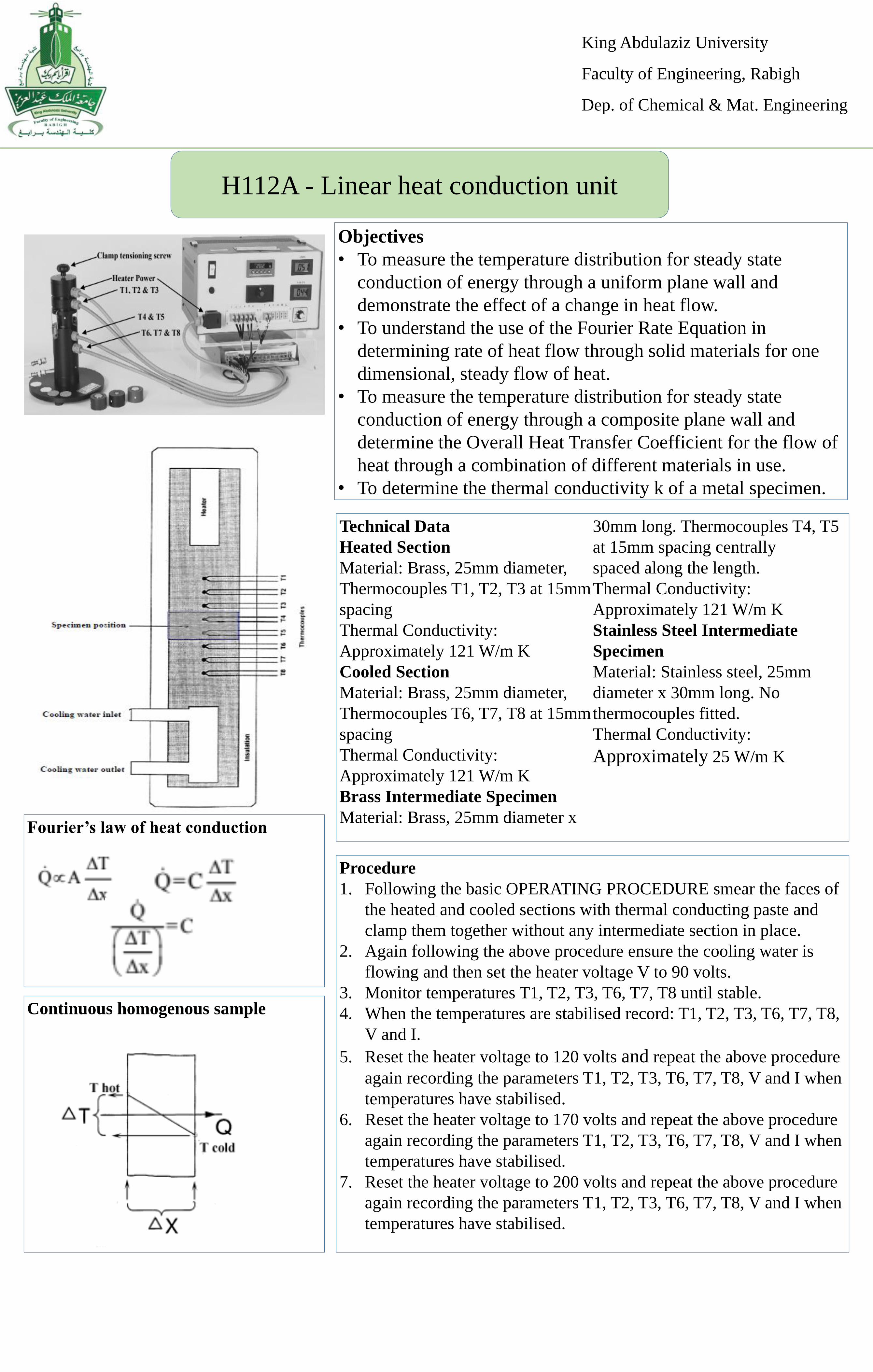
Continuous homogenous sample
Procedure
1. Following the basic OPERATING PROCEDURE smear the faces of
the heated and cooled sections with thermal conducting paste and
clamp them together without any intermediate section in place.
2. Again following the above procedure ensure the cooling water is
flowing and then set the heater voltage V to 90 volts.
3. Monitor temperatures T1, T2, T3, T6, T7, T8 until stable.
4. When the temperatures are stabilised record: T1, T2, T3, T6, T7, T8,
V and I.
5. Reset the heater voltage to 120 volts and repeat the above procedure
again recording the parameters T1, T2, T3, T6, T7, T8, V and I when
temperatures have stabilised.
6. Reset the heater voltage to 170 volts and repeat the above procedure
again recording the parameters T1, T2, T3, T6, T7, T8, V and I when
temperatures have stabilised.
7. Reset the heater voltage to 200 volts and repeat the above procedure
again recording the parameters T1, T2, T3, T6, T7, T8, V and I when
temperatures have stabilised.
Technical Data
Heated Section
Material: Brass, 25mm diameter,
Thermocouples T1, T2, T3 at 15mm
spacing
Thermal Conductivity:
Approximately 121 W/m K
Cooled Section
Material: Brass, 25mm diameter,
Thermocouples T6, T7, T8 at 15mm
spacing
Thermal Conductivity:
Approximately 121 W/m K
Brass Intermediate Specimen
Material: Brass, 25mm diameter x
30mm long. Thermocouples T4, T5
at 15mm spacing centrally
spaced along the length.
Thermal Conductivity:
Approximately 121 W/m K
Stainless Steel Intermediate
Specimen
Material: Stainless steel, 25mm
diameter x 30mm long. No
thermocouples fitted.
Thermal Conductivity:
Approximately 25 W/m K
Fourier’s law of heat conduction
King Abdulaziz University
Faculty of Engineering, Rabigh
Dep. of Chemical & Mat. Engineering
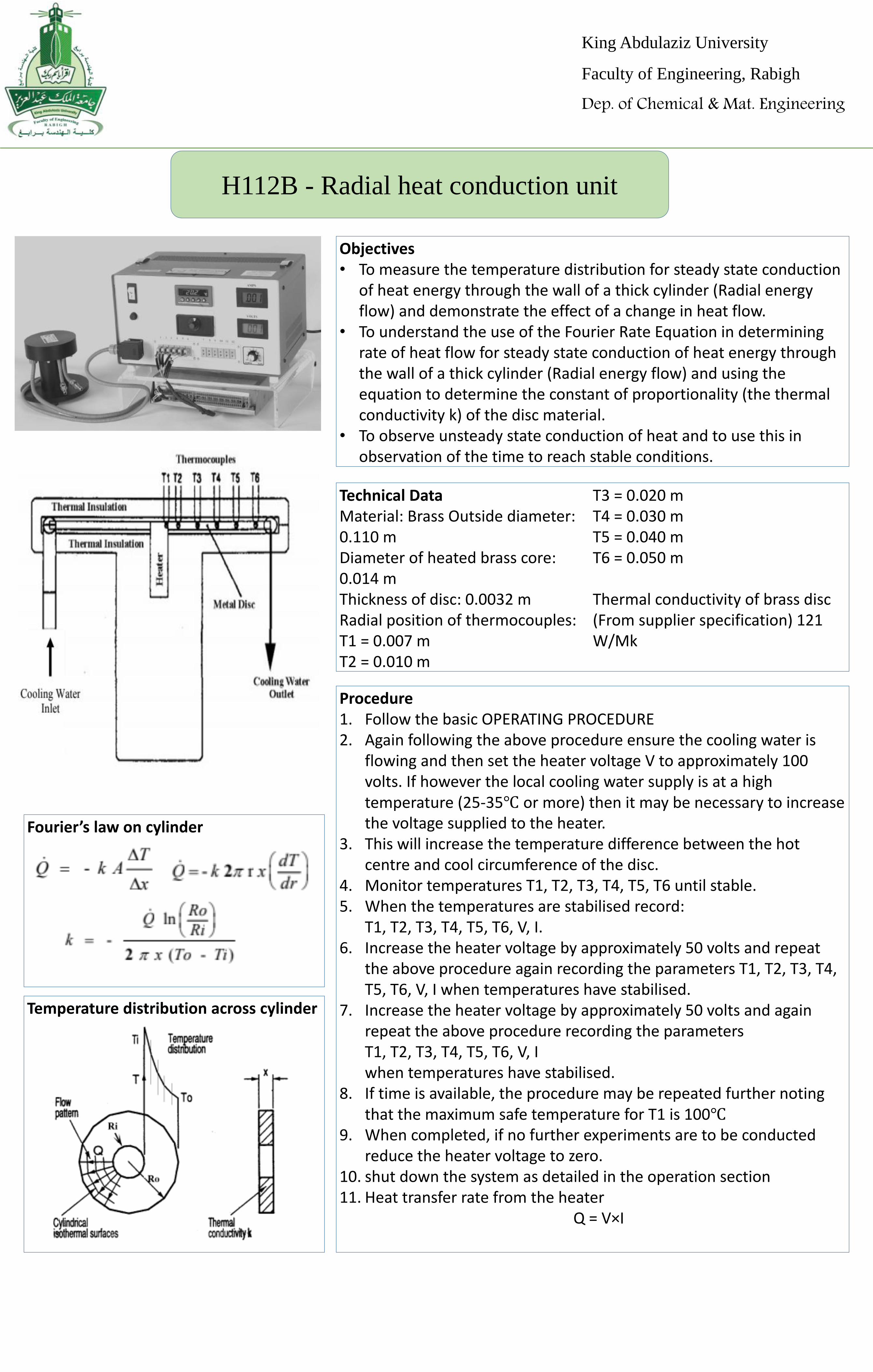
H112B - Radial heat conduction unit
Objectives • To measure the temperature distribution for steady state conduction
of heat energy through the wall of a thick cylinder (Radial energy flow) and demonstrate the effect of a change in heat flow.
• To understand the use of the Fourier Rate Equation in determining rate of heat flow for steady state conduction of heat energy through the wall of a thick cylinder (Radial energy flow) and using the equation to determine the constant of proportionality (the thermal conductivity k) of the disc material.
• To observe unsteady state conduction of heat and to use this in observation of the time to reach stable conditions.
Temperature distribution across cylinder
Procedure1. Follow the basic OPERATING PROCEDURE2. Again following the above procedure ensure the cooling water is
flowing and then set the heater voltage V to approximately 100 volts. If however the local cooling water supply is at a high temperature (25-35℃ or more) then it may be necessary to increase the voltage supplied to the heater.
3. This will increase the temperature difference between the hot centre and cool circumference of the disc.
4. Monitor temperatures T1, T2, T3, T4, T5, T6 until stable.5. When the temperatures are stabilised record:
T1, T2, T3, T4, T5, T6, V, I.6. Increase the heater voltage by approximately 50 volts and repeat
the above procedure again recording the parameters T1, T2, T3, T4, T5, T6, V, I when temperatures have stabilised.
7. Increase the heater voltage by approximately 50 volts and again repeat the above procedure recording the parameters T1, T2, T3, T4, T5, T6, V, I when temperatures have stabilised.
8. If time is available, the procedure may be repeated further noting that the maximum safe temperature for T1 is 100℃
9. When completed, if no further experiments are to be conducted reduce the heater voltage to zero.
10. shut down the system as detailed in the operation section11. Heat transfer rate from the heater
Q = V×I
Technical Data Material: Brass Outside diameter: 0.110 mDiameter of heated brass core: 0.014 mThickness of disc: 0.0032 mRadial position of thermocouples:T1 = 0.007 mT2 = 0.010 m
T3 = 0.020 mT4 = 0.030 mT5 = 0.040 mT6 = 0.050 m
Thermal conductivity of brass disc (From supplier specification) 121 W/Mk
Fourier’s law on cylinder

King Abdulaziz University
Faculty of Engineering, Rabigh
Dep. of Chemical & Mat. Engineering
H112C – Law of radiant heat transfer and
radiant heat exchange
6. Schematically this produces a system as
shown below.
7. Ensure that the radiation shield is in position
in the radiometer aperture and station the
radiometer in the 900mm position.
8. The radiometer should be left for several
minutes after handling with the radiation
shield in position to ensure that residual
heating has dissipated.
9. Follow the Operating procedure, but do not
increase the supply voltage to the heater
from the zero condition.
10. Monitor the W/m2 digital display and after
several minutes, the display should reach a
minimum.
11. Finally, ‘Auto-Zero’ the radiometer by
pressing the right hand Å button twice.
12. Leave the radiation shield in position and
rotate the voltage controller clockwise to
increase the voltage to maximum volts.
13. Select the T5 position on the temperature
selector switch and monitor the T5
temperature.
Objectives
• To show that the intensity of radiation on a surface is
inversely proportional to the square of the distance of the
surface from the source of radiation (To demonstrate the
inverse square law for thermal radiation)
• To show that the intensity of radiation varies as the fourth
power of the source temperature (To demonstrate the
Stefan-Boltzmann Law.)
• To show that the intensity of radiation measured by the
radiometer is directly related to the radiation emitted from
a source by the view factor between the radiometer and the
source.
• To determine the emissivity of radiating surfaces with
different finishes, namely polished and grey (silver
anodised) compared with matt black.
• To demonstrate how the emissivity of radiating surfaces in
close proximity to each other will affect the surface
temperatures and heat exchanged.
• To show that the illuminance of a surface is inversely
proportional to the square of the distance of the surface
from the light source.
Procedure
1. Following the basic OPERATING PROCEDURE and
INSTALLATION PROCEDURE
2. Install the heated plate C1(10) at the left hand side of the
track and install the radiometer C1(12) on the right hand
carriage C1(2).
3. No items are installed in the left hand carriage for this
experiment but one of the black plates should be placed
on the bench and connected to thermocouple socket T4.
Technical Data
Stefan-Boltzmann Constant
σ = 5.67 x 10⁻⁸ W/m2 K4
Temperature locations
T1 Black Plate
T2 Black Plate
T3 Grey Plate
T4 Polished Plate
T5 Heated Plate

King Abdulaziz University
Faculty of Engineering, Rabigh
Dep. of Chemical & Mat. Engineering
H112D - Combined convection and
radiation
Objectives
• Determination of the combined (radiation and convection) heat
transfer (Qr + Qc) from a horizontal cylinder in natural convection
over a wide range of power input and corresponding surface
temperature.
• Measuring the domination of the convective heat transfer coefficient
hc at low surface temperatures and the domination of the radiation
heat transfer coefficient hr at high surface temperatures.
• Determination of the effect of forced convection on the heat transfer
from the cylinder at varying air velocities.
• Determination of the local heat transfer coefficient around the
cylinder.
Cylinder
Procedure
1. Following the basic OPERATING PROCEDURE ensure that the
heated cylinder is located in its holder at the top of the duct and that
the cylinder is rotated so that the thermocouple location is on the
side of the cylinder. This is shown schematically below.
2. Follow the Operating Procedure. Rotate the voltage controller to give
a 50-volt reading.
3. Select the temperature position T2 using the rotary selector switch
and monitor the temperature.
4. Open the throttle butterfly on the fan intake but do not turn on the
fan switch, as the fan will not be used for this experiment.
5. When T2 has reached a steady state temperature record the
following:
T1, T2, V, I.
6. Increase the voltage controller to give an 80-volt reading, monitor T2
for stability and repeat the readings.
7. Increase the voltage controller to give a 120-volt reading, monitor T2
for stability and repeat the readings.
8. Increase the voltage controller to give a 150-volt reading, monitor T2
for stability and repeat the readings.
9. Finally, increase the voltage controller to give approximately a 185-
volt reading, monitor T2 for stability and repeat the readings.
Technical Data
Cylinder diameter D = 0.01m
Cylinder Heated Length L = 0.07m
Cylinder effective heated area
As = 0.0022m2
Effective air velocity local to
cylinder due to blockage effect Ue =
Ua x 1.22
Heat lost due to natural convection
Radiant component
Total heat transfer from the cylinder
Overall heat transfer coefficient
King Abdulaziz University
Faculty of Engineering, Rabigh
Dep. of Chemical & Mat. Engineering
H112E - Extended surface heat transfer
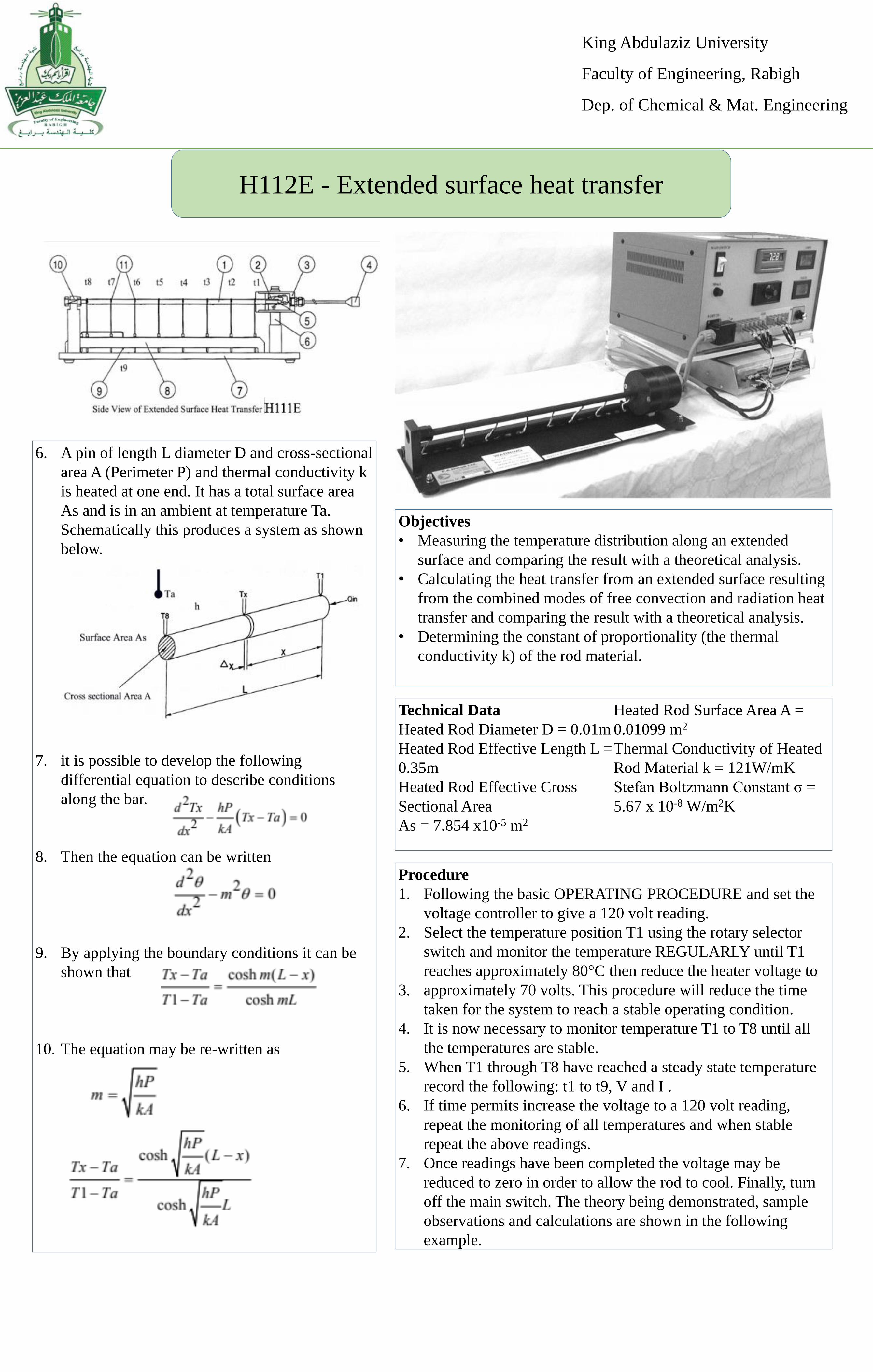
6. A pin of length L diameter D and cross-sectional
area A (Perimeter P) and thermal conductivity k
is heated at one end. It has a total surface area
As and is in an ambient at temperature Ta.
Schematically this produces a system as shown
below.
7. it is possible to develop the following
differential equation to describe conditions
along the bar.
8. Then the equation can be written
9. By applying the boundary conditions it can be
shown that
10. The equation may be re-written as
Objectives
• Measuring the temperature distribution along an extended
surface and comparing the result with a theoretical analysis.
• Calculating the heat transfer from an extended surface resulting
from the combined modes of free convection and radiation heat
transfer and comparing the result with a theoretical analysis.
• Determining the constant of proportionality (the thermal
conductivity k) of the rod material.
Procedure
1. Following the basic OPERATING PROCEDURE and set the
voltage controller to give a 120 volt reading.
2. Select the temperature position T1 using the rotary selector
switch and monitor the temperature REGULARLY until T1
reaches approximately 80°C then reduce the heater voltage to
3. approximately 70 volts. This procedure will reduce the time
taken for the system to reach a stable operating condition.
4. It is now necessary to monitor temperature T1 to T8 until all
the temperatures are stable.
5. When T1 through T8 have reached a steady state temperature
record the following: t1 to t9, V and I .
6. If time permits increase the voltage to a 120 volt reading,
repeat the monitoring of all temperatures and when stable
repeat the above readings.
7. Once readings have been completed the voltage may be
reduced to zero in order to allow the rod to cool. Finally, turn
off the main switch. The theory being demonstrated, sample
observations and calculations are shown in the following
example.
Technical Data
Heated Rod Diameter D = 0.01m
Heated Rod Effective Length L =
0.35m
Heated Rod Effective Cross
Sectional Area
As = 7.854 x10⁻⁵ m2
Heated Rod Surface Area A =
0.01099 m2
Thermal Conductivity of Heated
Rod Material k = 121W/mK
Stefan Boltzmann Constant σ =
5.67 x 10⁻⁸ W/m2K
King Abdulaziz University
Faculty of Engineering, Rabigh
Dep. of Chemical & Mat. Engineering
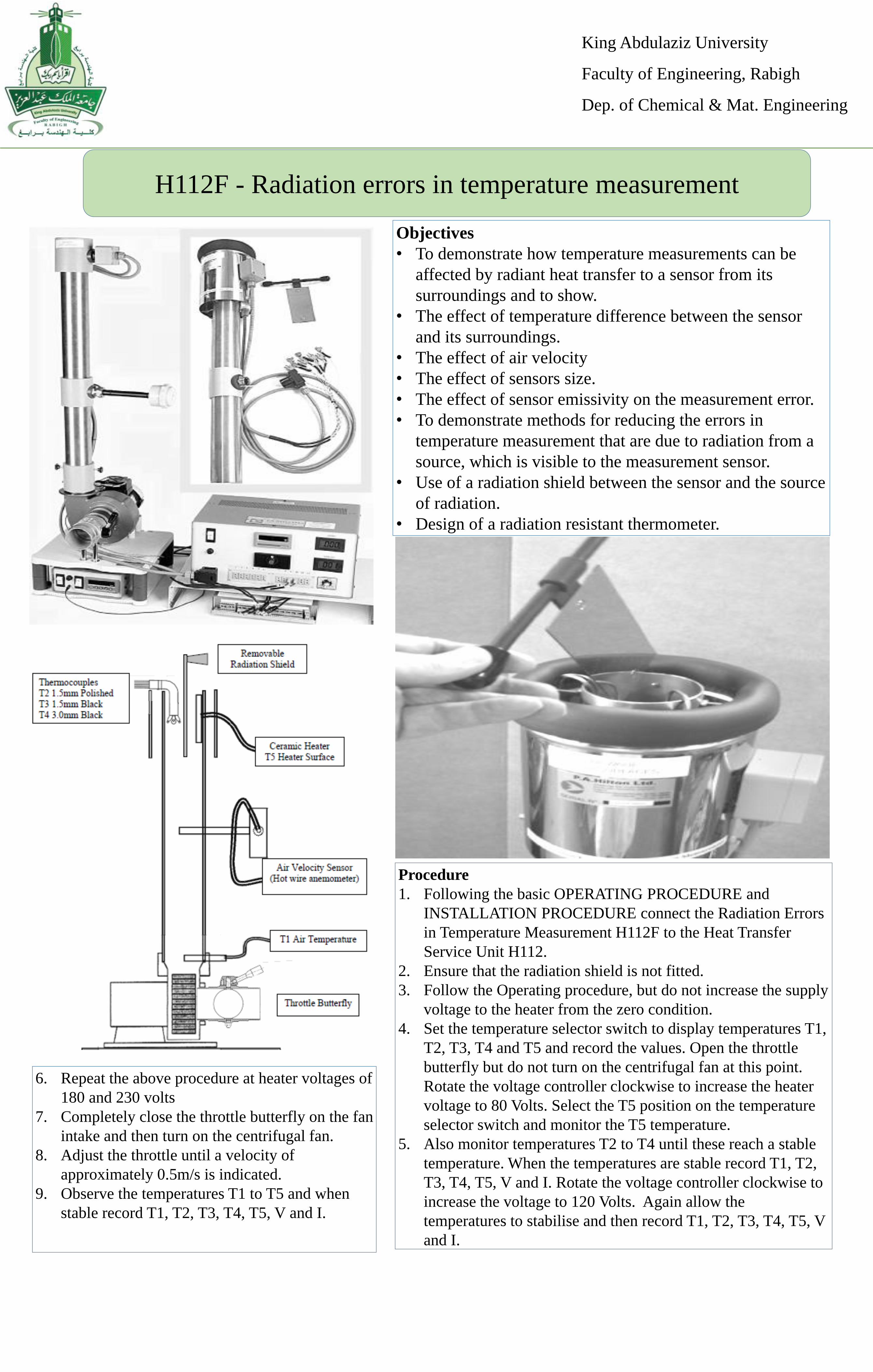
H112F - Radiation errors in temperature measurement
6. Repeat the above procedure at heater voltages of
180 and 230 volts
7. Completely close the throttle butterfly on the fan
intake and then turn on the centrifugal fan.
8. Adjust the throttle until a velocity of
approximately 0.5m/s is indicated.
9. Observe the temperatures T1 to T5 and when
stable record T1, T2, T3, T4, T5, V and I.
Objectives
• To demonstrate how temperature measurements can be
affected by radiant heat transfer to a sensor from its
surroundings and to show.
• The effect of temperature difference between the sensor
and its surroundings.
• The effect of air velocity
• The effect of sensors size.
• The effect of sensor emissivity on the measurement error.
• To demonstrate methods for reducing the errors in
temperature measurement that are due to radiation from a
source, which is visible to the measurement sensor.
• Use of a radiation shield between the sensor and the source
of radiation.
• Design of a radiation resistant thermometer.
Procedure
1. Following the basic OPERATING PROCEDURE and
INSTALLATION PROCEDURE connect the Radiation Errors
in Temperature Measurement H112F to the Heat Transfer
Service Unit H112.
2. Ensure that the radiation shield is not fitted.
3. Follow the Operating procedure, but do not increase the supply
voltage to the heater from the zero condition.
4. Set the temperature selector switch to display temperatures T1,
T2, T3, T4 and T5 and record the values. Open the throttle
butterfly but do not turn on the centrifugal fan at this point.
Rotate the voltage controller clockwise to increase the heater
voltage to 80 Volts. Select the T5 position on the temperature
selector switch and monitor the T5 temperature.
5. Also monitor temperatures T2 to T4 until these reach a stable
temperature. When the temperatures are stable record T1, T2,
T3, T4, T5, V and I. Rotate the voltage controller clockwise to
increase the voltage to 120 Volts. Again allow the
temperatures to stabilise and then record T1, T2, T3, T4, T5, V
and I.
King Abdulaziz University
Faculty of Engineering, Rabigh
Dep. of Chemical & Mat. Engineering
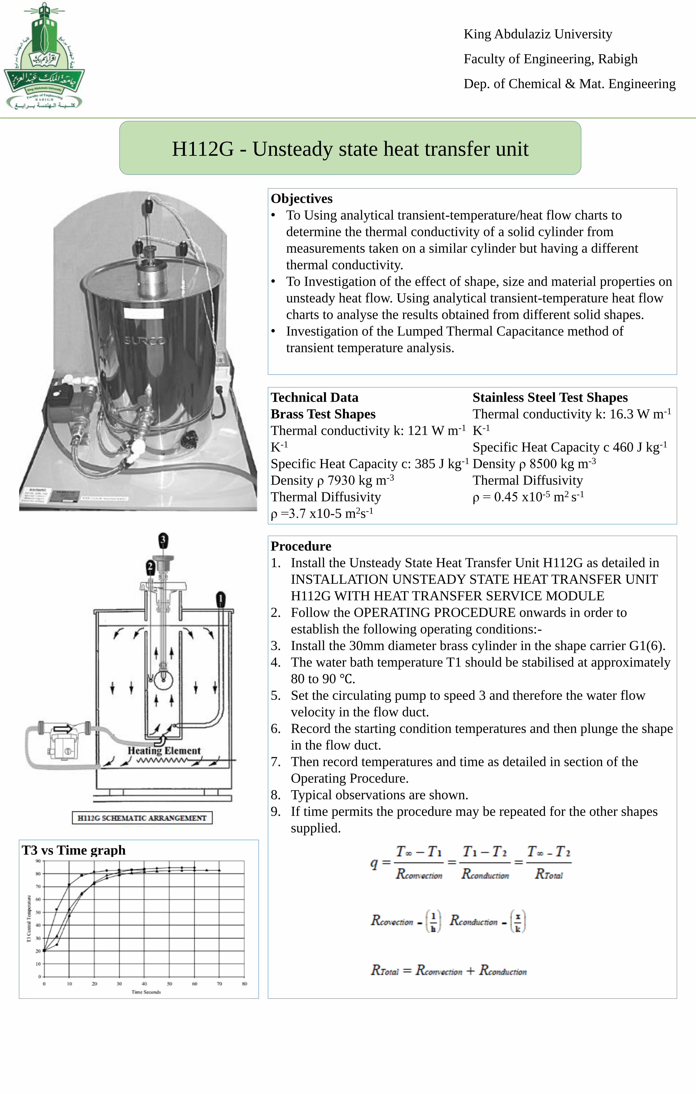
H112G - Unsteady state heat transfer unit
Objectives
• To Using analytical transient-temperature/heat flow charts to
determine the thermal conductivity of a solid cylinder from
measurements taken on a similar cylinder but having a different
thermal conductivity.
• To Investigation of the effect of shape, size and material properties on
unsteady heat flow. Using analytical transient-temperature heat flow
charts to analyse the results obtained from different solid shapes.
• Investigation of the Lumped Thermal Capacitance method of
transient temperature analysis.
T3 vs Time graph
Procedure
1. Install the Unsteady State Heat Transfer Unit H112G as detailed in
INSTALLATION UNSTEADY STATE HEAT TRANSFER UNIT
H112G WITH HEAT TRANSFER SERVICE MODULE
2. Follow the OPERATING PROCEDURE onwards in order to
establish the following operating conditions:-
3. Install the 30mm diameter brass cylinder in the shape carrier G1(6).
4. The water bath temperature T1 should be stabilised at approximately
80 to 90 ℃.
5. Set the circulating pump to speed 3 and therefore the water flow
velocity in the flow duct.
6. Record the starting condition temperatures and then plunge the shape
in the flow duct.
7. Then record temperatures and time as detailed in section of the
Operating Procedure.
8. Typical observations are shown.
9. If time permits the procedure may be repeated for the other shapes
supplied.
Technical Data
Brass Test Shapes
Thermal conductivity k: 121 W m-1
K-1
Specific Heat Capacity c: 385 J kg-1
Density ρ 7930 kg m-3
Thermal Diffusivity
ρ =3.7 x10⁻⁵ m2s-1
Stainless Steel Test Shapes
Thermal conductivity k: 16.3 W m-1
K-1
Specific Heat Capacity c 460 J kg-1
Density ρ 8500 kg m-3
Thermal Diffusivity
ρ = 0.45 x10⁻⁵ m2 s-1
King Abdulaziz University
Faculty of Engineering, Rabigh
Dep. of Chemical & Mat. Engineering
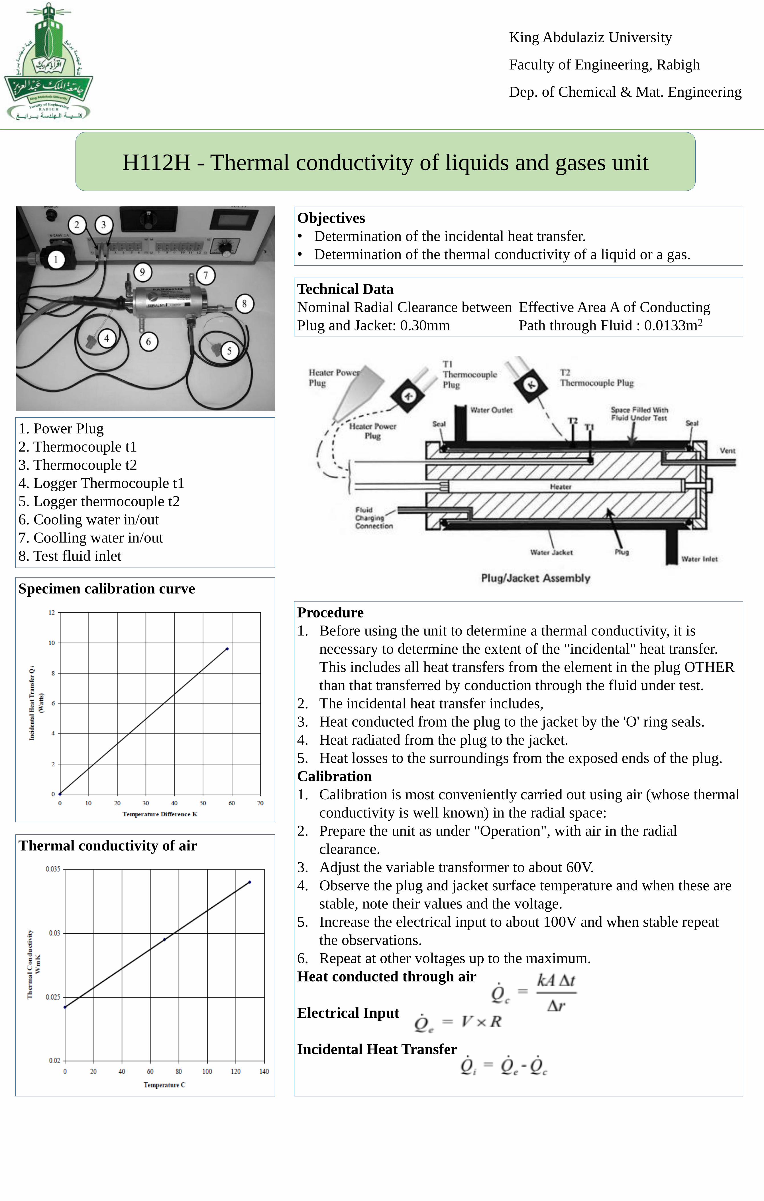
H112H - Thermal conductivity of liquids and gases unit
Objectives
• Determination of the incidental heat transfer.
• Determination of the thermal conductivity of a liquid or a gas.
Thermal conductivity of air
Procedure
1. Before using the unit to determine a thermal conductivity, it is
necessary to determine the extent of the "incidental" heat transfer.
This includes all heat transfers from the element in the plug OTHER
than that transferred by conduction through the fluid under test.
2. The incidental heat transfer includes,
3. Heat conducted from the plug to the jacket by the 'O' ring seals.
4. Heat radiated from the plug to the jacket.
5. Heat losses to the surroundings from the exposed ends of the plug.
Calibration
1. Calibration is most conveniently carried out using air (whose thermal
conductivity is well known) in the radial space:
2. Prepare the unit as under "Operation", with air in the radial
clearance.
3. Adjust the variable transformer to about 60V.
4. Observe the plug and jacket surface temperature and when these are
stable, note their values and the voltage.
5. Increase the electrical input to about 100V and when stable repeat
the observations.
6. Repeat at other voltages up to the maximum.
Heat conducted through air
Electrical Input
Incidental Heat Transfer
Technical Data
Nominal Radial Clearance between
Plug and Jacket: 0.30mm
Effective Area A of Conducting
Path through Fluid : 0.0133m2
1. Power Plug
2. Thermocouple t1
3. Thermocouple t2
4. Logger Thermocouple t1
5. Logger thermocouple t2
6. Cooling water in/out
7. Coolling water in/out
8. Test fluid inlet
Specimen calibration curve
King Abdulaziz University
Faculty of Engineering, Rabigh
Dep. of Chemical & Mat. Engineering
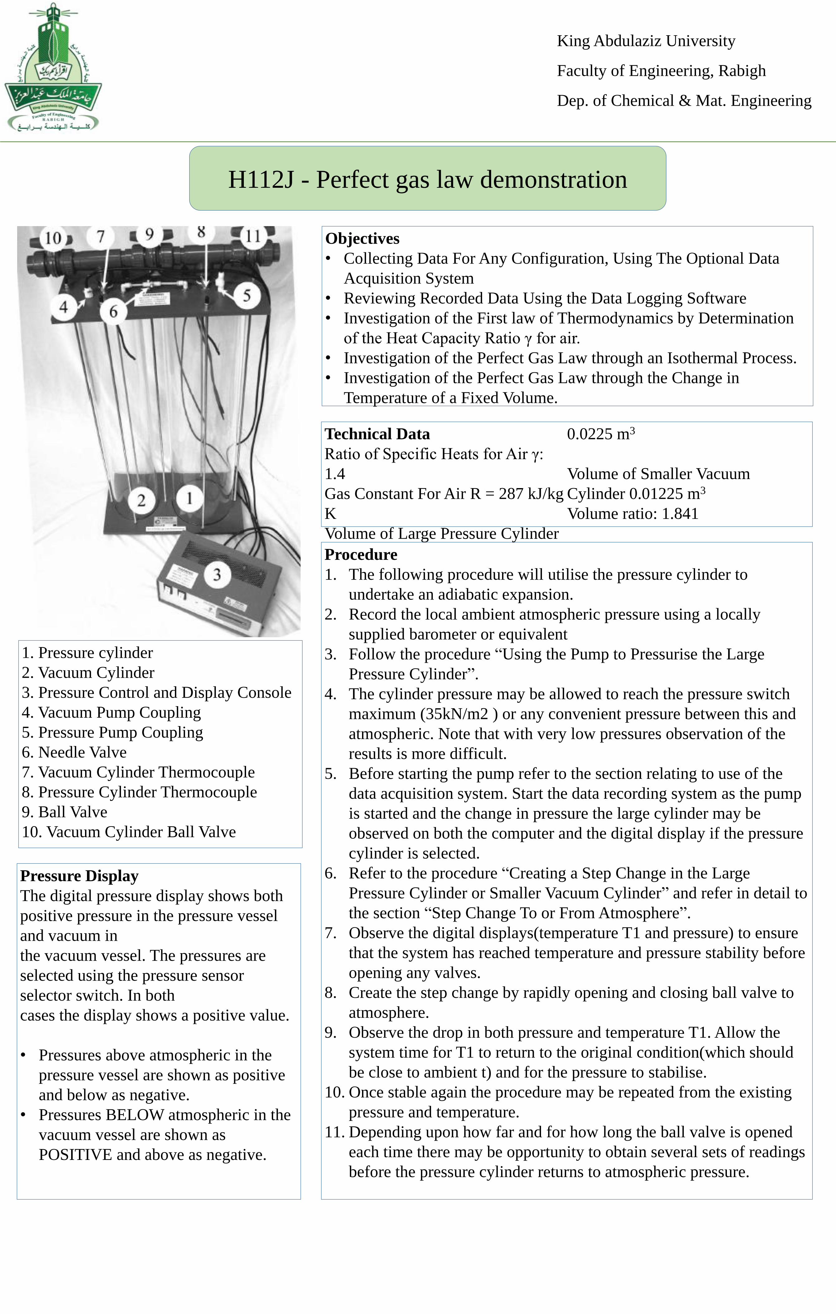
H112J - Perfect gas law demonstration
Objectives
• Collecting Data For Any Configuration, Using The Optional Data
Acquisition System
• Reviewing Recorded Data Using the Data Logging Software
• Investigation of the First law of Thermodynamics by Determination
of the Heat Capacity Ratio γ for air.
• Investigation of the Perfect Gas Law through an Isothermal Process.
• Investigation of the Perfect Gas Law through the Change in
Temperature of a Fixed Volume.
Pressure Display
The digital pressure display shows both
positive pressure in the pressure vessel
and vacuum in
the vacuum vessel. The pressures are
selected using the pressure sensor
selector switch. In both
cases the display shows a positive value.
• Pressures above atmospheric in the
pressure vessel are shown as positive
and below as negative.
• Pressures BELOW atmospheric in the
vacuum vessel are shown as
POSITIVE and above as negative.
Procedure
1. The following procedure will utilise the pressure cylinder to
undertake an adiabatic expansion.
2. Record the local ambient atmospheric pressure using a locally
supplied barometer or equivalent
3. Follow the procedure “Using the Pump to Pressurise the Large
Pressure Cylinder”.
4. The cylinder pressure may be allowed to reach the pressure switch
maximum (35kN/m2 ) or any convenient pressure between this and
atmospheric. Note that with very low pressures observation of the
results is more difficult.
5. Before starting the pump refer to the section relating to use of the
data acquisition system. Start the data recording system as the pump
is started and the change in pressure the large cylinder may be
observed on both the computer and the digital display if the pressure
cylinder is selected.
6. Refer to the procedure “Creating a Step Change in the Large
Pressure Cylinder or Smaller Vacuum Cylinder” and refer in detail to
the section “Step Change To or From Atmosphere”.
7. Observe the digital displays(temperature T1 and pressure) to ensure
that the system has reached temperature and pressure stability before
opening any valves.
8. Create the step change by rapidly opening and closing ball valve to
atmosphere.
9. Observe the drop in both pressure and temperature T1. Allow the
system time for T1 to return to the original condition(which should
be close to ambient t) and for the pressure to stabilise.
10. Once stable again the procedure may be repeated from the existing
pressure and temperature.
11. Depending upon how far and for how long the ball valve is opened
each time there may be opportunity to obtain several sets of readings
before the pressure cylinder returns to atmospheric pressure.
Technical Data
Ratio of Specific Heats for Air γ:
1.4
Gas Constant For Air R = 287 kJ/kg
K
Volume of Large Pressure Cylinder
0.0225 m3
Volume of Smaller Vacuum
Cylinder 0.01225 m3
Volume ratio: 1.841
1. Pressure cylinder
2. Vacuum Cylinder
3. Pressure Control and Display Console
4. Vacuum Pump Coupling
5. Pressure Pump Coupling
6. Needle Valve
7. Vacuum Cylinder Thermocouple
8. Pressure Cylinder Thermocouple
9. Ball Valve
10. Vacuum Cylinder Ball Valve
King Abdulaziz University
Faculty of Engineering, Rabigh
Dep. of Chemical & Mat. Engineering
H112M - Marcet boiler
Objectives
• Investigation of the pressure-temperature relationship for
Water/steam.
• Investigation of the Clausius- Clapeyron equation using the Pressure-
temperature relationship for steam.
• Investigation of steam quality by throttling.
Procedure
1. Refer to the operating procedure. Ensure in particular that the boiler
contains sufficient water.
2. Record the local ambient atmospheric pressure using a locally
supplied barometer or equivalent. Record the starting condition
Temperature T1 and Pressure.
3. If the pressure is to be recorded from a sub-atmospheric pressure
then refer to the “Second Time Use When the Boiler is In Vacuum”
procedure.
4. Increase the heater to full power and monitor the increasing
temperature and pressure. At relevant intervals record both the
pressure and temperature.
5. It is recommended that either whole units of pressure or whole units
of temperature are selected as the recording points as this makes
reference to steam tables easier.
Pressure
1. The gauge pressure indicated by the bourdon tube pressure gauge is
“relative” to atmospheric pressure.
2. Atmospheric pressure varies depending upon weather conditions and
location(sea level or high altitude) and therefore it would be
impractical to present the pressure-temperature relationship for water
in terms of gauge pressure as the readings would vary.
3. Therefore it is normal to refer pressures to an absolute vacuum. This
can be achieved either by using a pressure gauge that is internally
evacuated and sealed or by adding the local atmospheric pressure to
the pressure measured by a standard pressure gauge.1. Boiler
2. Sight Glass
3. Pressure Gauge
4. Throttle Valve
5. Pressure Switch
6. Safety Valve
7. Water fill / Drain
8. Throttle Valve Vent Coupling
9. Safety Valve Vent Coupling
10. Pressure Transducer (*Only fitted if
HC112MA is Purchased).
Pressure Switch
The pressure switch is factory set to
operate at or below 900kN/m2
gauge pressure. This turns off the
heater inside the boiler.
King Abdulaziz University
Faculty of Engineering, Rabigh
Dep. of Chemical & Mat. Engineering
H112P - Free and forced convection from flat, finned and pinned plates
Objectives
• To Demonstrate the Relationship Between Power Input and Surface
Temperature in Free Convection
• To Demonstrate the Relationship Between Power Input and Surface
Temperature in Forced Convection.
• To Demonstrate the use of Extended Surfaces to Improve Heat
Transfer From the Surface.
• To Determine the Temperature Distribution Along an Extended
Surface.
Procedure
1. Ensure the instrument console main switch is sin the off position.
Ensure the fan is switched off.
2. For the natural convection experiments the fan will not be used.
3. If the flat (pinned or finned) plate is not in position, open the toggle
clamps. Replace with the flat(pinned or finned) plate and close the
toggle clamps. Note that with the plate heat exchangers the power
leads exit from the top of the plates. Refer to the diagram.
4. No air velocity will be measurable under natural convection
conditions unless specialized instrumentation is available.
5. Switch on the main switch and set the heater voltage to minimum.
6. The objective with the steady state method is to obtain the same T1
surface temperature on each of the heat exchangers and determine
the steady state power input required to achieve this. From factory
tests under “typical” conditions the following heat inputs were
required to maintain T1.
7. When the temperature T1 has stabilised(this may take 10’s of
minutes) record the actual temperature T1, the actual voltage V and
the ambient air temperature T9. If either the Finned or Pinned plates
are in position the pin temperatures (T2,T3,T4) or fin temperatures
(T2, T3, T4) may be recorded.
8. Before removing the heat exchanger from the duct turn on the fan
and cool the heat exchanger .
9. Note that this cooling procedure may be used to quickly demonstrate
to students the increased heat transfer coefficient due to forced
convection if the voltage setting is left at the natural convection
condition and the fan turned on to give maximum flow.
10. T1 will be seen to rapidly fall from the natural convection condition.
11. Finally reduce the heater voltage to zero and allow to cool before
removing the plate from the tunnel and replacing with one of the
alternative plates.
12. Test results from the steady state method are obtained.
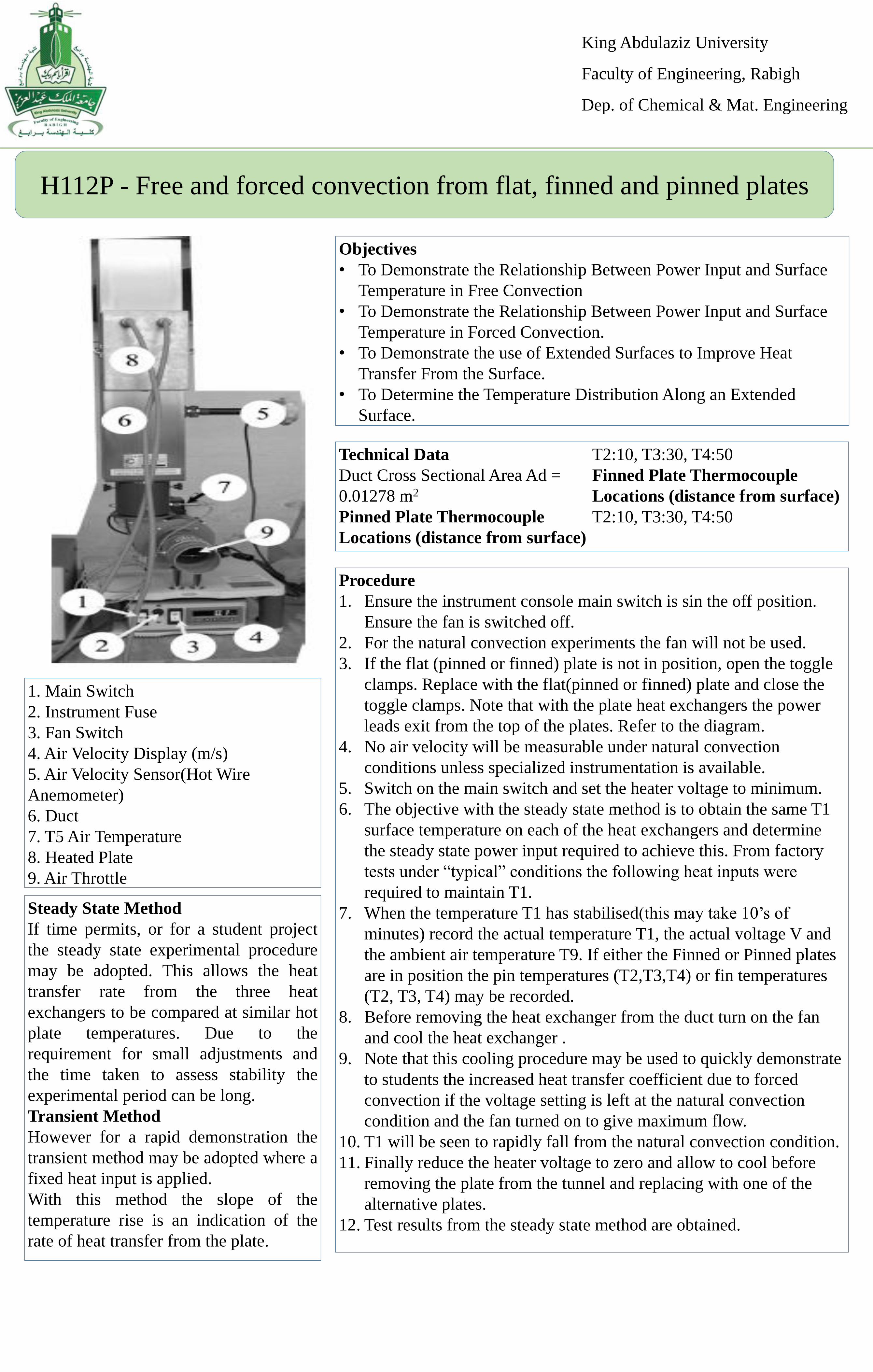
1. Main Switch
2. Instrument Fuse
3. Fan Switch
4. Air Velocity Display (m/s)
5. Air Velocity Sensor(Hot Wire
Anemometer)
6. Duct
7. T5 Air Temperature
8. Heated Plate
9. Air Throttle
Steady State Method
If time permits, or for a student project
the steady state experimental procedure
may be adopted. This allows the heat
transfer rate from the three heat
exchangers to be compared at similar hot
plate temperatures. Due to the
requirement for small adjustments and
the time taken to assess stability the
experimental period can be long.
Transient Method
However for a rapid demonstration the
transient method may be adopted where a
fixed heat input is applied.
With this method the slope of the
temperature rise is an indication of the
rate of heat transfer from the plate.
Technical Data
Duct Cross Sectional Area Ad =
0.01278 m2
Pinned Plate Thermocouple
Locations (distance from surface)
T2:10, T3:30, T4:50
Finned Plate Thermocouple
Locations (distance from surface)
T2:10, T3:30, T4:50
King Abdulaziz University
Faculty of Engineering, Rabigh
Dep. of Chemical & Mat. Engineering
H112Q - Thermoelectric heat pump
Objectives
• Investigation of the effects upon the surface temperature of either face
of the module with increasing power. (Peltier Effect)
• Investigation of the effect upon heat transfer direction of reversing the
polarity of the power supply to the module. (Thomson or Lenz
Effect).
• Investigation of the variation in open circuit voltage across the
module due to the variation in surface temperature difference.
(Seebeck Effect).
• Investigation of the power generating performance of the module with
a steady load and increasing temperature difference.
• Estimation of the coefficient of performance of the module when
acting as a refrigerator.
Procedure
1. It is assumed that the H112Q Thermoelectric Heat Pump Module has
being installed and commissioned.
2. The following experiment demonstrates that if supplied with DC
power the peltier module will cool the upper block.
3. If no external heat is supplied (by the cartridge heater in the upper
block) then the block temperature(T1) will reach a very low value.
4. Turn on the main switch of the H112 Heat Transfer Service unit and
turn the H112 Heater power control to zero (or disconnect the multi-
way plug).
5. Ensure cooling water is flowing through the water cooling
connections to the lower block.
6. Ensure that the DC Power Connectors are red to red and black to
black both ends.
7. Ensure the Load switch is down(on) and the Cooling/generating
switch is set to cooling.
8. Turn on the H112Q control console main switch and set the DC
power control to a low voltage(e.g. 0.5V on the dc voltmeter).
9. Monitor the top block temperature T1. When T1 and T2 are stable
record T1 through to T4 and the DC current and Voltage.
10. Increase the DC voltage in small increments and repeat the
monitoring procedure, recording the data when stable. Repeat the
procedure until the maximum Dc voltage is reached.
11. As may be seen as the supply voltage and current are increased the
upper block temperature t1 reduces considerably as heat is extracted
from the block.
12. The voltage may be increased if required but care must be taken as
the top block(being heated) does not have any water cooling.
13. As may be seen, if compared with the typical data the T1 and T2
temperature trends are reversed showing that the heat transfer has
been reversed.
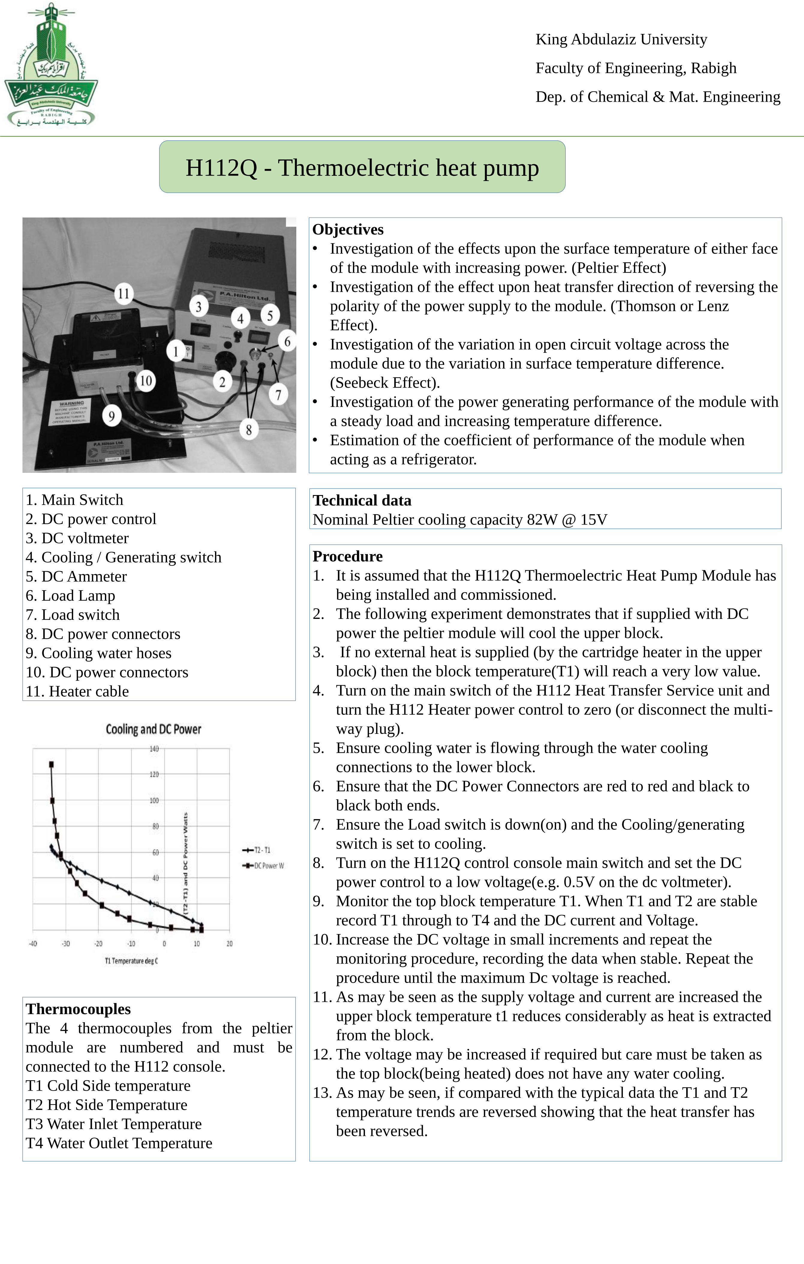
1. Main Switch
2. DC power control
3. DC voltmeter
4. Cooling / Generating switch
5. DC Ammeter
6. Load Lamp
7. Load switch
8. DC power connectors
9. Cooling water hoses
10. DC power connectors
11. Heater cable
Thermocouples
The 4 thermocouples from the peltier
module are numbered and must be
connected to the H112 console.
T1 Cold Side temperature
T2 Hot Side Temperature
T3 Water Inlet Temperature
T4 Water Outlet Temperature
Technical data
Nominal Peltier cooling capacity 82W @ 15V

King Abdulaziz University
Faculty of Engineering, Rabigh
Dep. of Chemical & Mat. Engineering
H112R - Stirling cycle engine
Objectives
• Demonstration of a direct conversion of heat energy into shaft power
using a Stirling Cycle.
• Investigation of the Stirling cycle performance under load.
• Investigation of the parameters affecting the cycle performance and
cycle efficiency.
Procedure
1. The following experiment demonstrates the way in which direct
heating of the air charge in the Stirling engine results in a mechanical
power output.
2. Turn on the main switch of the H112 Heat Transfer Service unit and
turn the H112 Heater power control to zero.
3. Ensure cooling water is flowing through the water cooling
connections.
4. Turn the heater power control on the H112 Transfer Service unit
slowly clockwise until a current of approximately 0.500 amps is
shown on the H112 Ammeter.
5. Monitor the temperature of the heater TH on the heater temperature
display as this approaches 350°C increase or reduce the power input
to maintain the TH temperature in the 350-380°C range.
6. Now ensure that the load adjuster is set so that the belt brake is
loose. Rotate the flywheel in a clockwise direction, as before and the
pressure of the air acting on the power piston should be felt assisting
in rotation of the flywheel as the piston moves outwards along the
power cylinder. This is the effect of the expanding-heated air moved
by the displacer.
7. If the flywheel is spun in a clockwise direction the engine should
turn slowly and reach a stable speed.
8. Now slightly increase the heater power so that the heater temperature
TH increases slightly and observe the rotational speed of the engine.
This should slowly increase with TH.
9. Though the belt brake is not being used to load the engine it can be
seen that the heat put into the system by the electric heater is being
converted to mechanical energy in order to maintain rotation of the
flywheel.
10. In this condition the engine is only generating power to overcome its
own internal friction.
11. Note that the heater has a maximum temperature limit of 600°C and
when the heater temperature display
12. reaches 600°C there will be an audible click from the display . At
that point the current displayed on the digital current meter will drop
to 0000 as the power is disconnected. The power is re-connected
automatically as the temperature falls to below 599°C.
1. Stirling cycle engine
2. Load cell display
3. Tachometer indicator
4. Heater temperature display
5. H112R heater power connection
6. Heater terminal enclosure
7. heater cylinder
8. Cooling water inlet
9. Flywheel
10. Belt brake
11. Power cylinder
12. Load Adjuster
13. Crankshaft
15. Cooling water drain
16. cold side thermocouple
17. tachometer sensor (hidden)
The Torque Φ developed by the engine
can be calculated
The shaft power W can be calculated
from
Technical data
Radius of Belt Brake Wheel r = 20mm
King Abdulaziz University
Faculty of Engineering, Rabigh
Dep. of Chemical & Mat. Engineering
H112S - Boiling heat transfer module
Objectives
• Visual demonstration of convective, nucleate and film boiling.
• Determination of heat flux and surface heat transfer coefficient up to
and beyond the critical
• condition at constant pressure.
• Investigation of the effect of pressure on critical heat flux.
• Demonstration of filmwise condensation and measurement of overall
heat transfer coefficient.
• Demonstration of the cause of liquid carry over or priming in boilers.
• Determination of the pressure temperature relationship of a pure
substance.
• Investigation of the effect of air in a condenser.
• Demonstration of the law of partial pressures.
Procedure
1. Observe the normal operating procedure before starting this
procedure.
2. Turn on the electrical and water supplies and adjust both to very low
settings (<20 Watts). Allow the digital t1 temperature indicator to
stabilise. Observe this and the liquid temperature t2 at frequent
intervals.
3. It is assumed that the chamber is air free at this point(observed
pressure on the pressure gauge = Saturation pressure at t2).
4. Carefully watch the liquid surrounding the heated cylinder.
Convection currents will be observed, and at the same time liquid
will be seen to collect and drip on the condenser coils, indicating that
evaporation is proceeding although at a low rate. Increase the heat
input in increments by adjusting the heater control , keeping the
vapour pressure at any desired constant value by adjusting the
condenser water flow rate by the water flow control and meter.
5. Nucleate boiling will soon start and will increase until vigorous
boiling is seen, the temperature difference (t1-t2) between the liquid
and metal being still quite moderate (<20K).
6. Increase the heat input, and at between 300 and 400 Watts the nature
of the boiling will be seen to change dramatically and at the same
time the metal-liquid temperature difference will rise quickly.
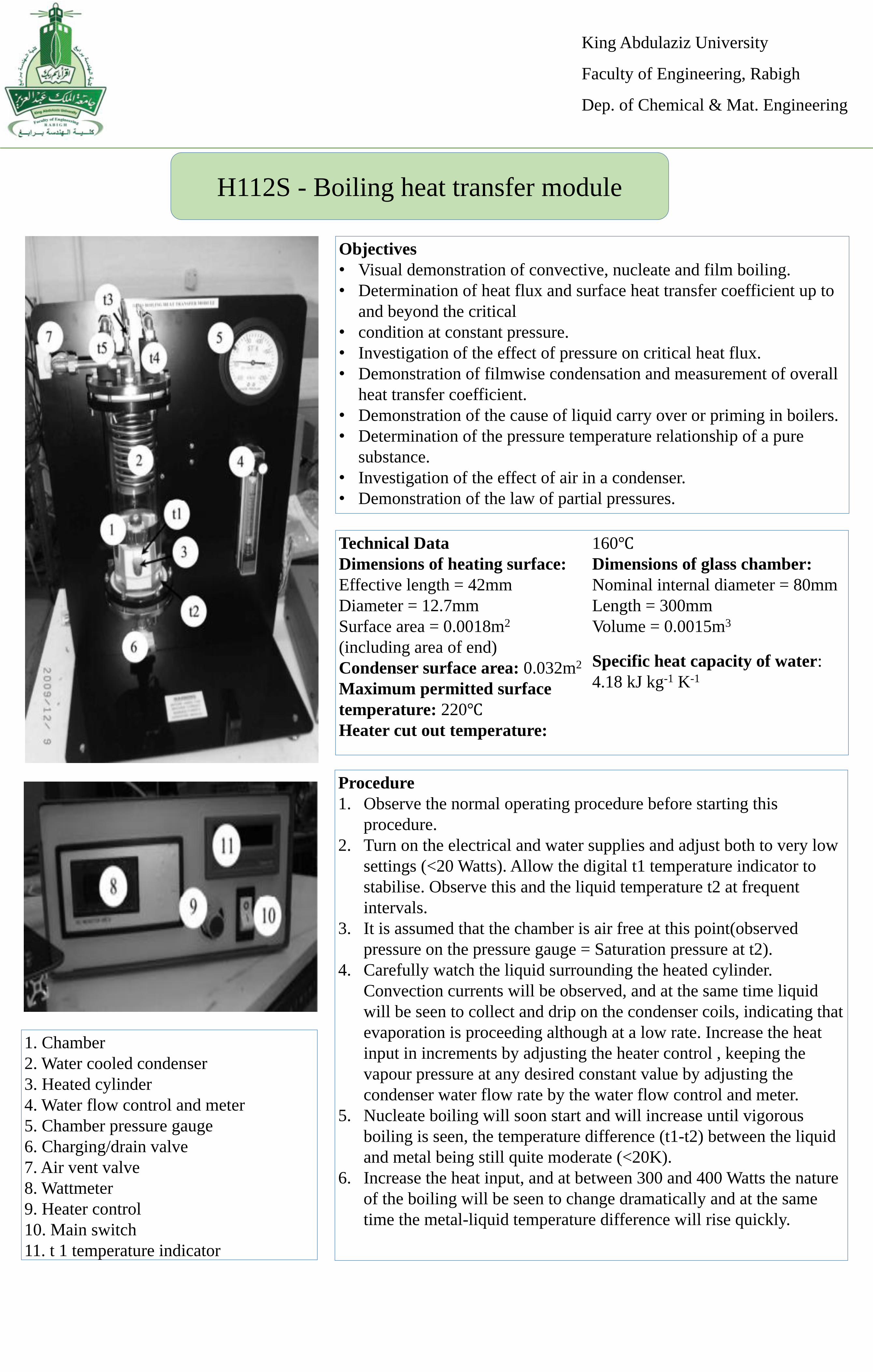
1. Chamber
2. Water cooled condenser
3. Heated cylinder
4. Water flow control and meter
5. Chamber pressure gauge
6. Charging/drain valve
7. Air vent valve
8. Wattmeter
9. Heater control
10. Main switch
11. t 1 temperature indicator
Technical Data
Dimensions of heating surface:
Effective length = 42mm
Diameter = 12.7mm
Surface area = 0.0018m2
(including area of end)
Condenser surface area: 0.032m2
Maximum permitted surface
temperature: 220℃Heater cut out temperature:
160℃Dimensions of glass chamber:
Nominal internal diameter = 80mm
Length = 300mm
Volume = 0.0015m3
Specific heat capacity of water:
4.18 kJ kg-1 K-1
King Abdulaziz University
Faculty of Engineering, Rabigh
Dep. of Chemical & Mat. Engineering
H102A - Concentric heat tube exchanger
Technical Data
• Inner tube material: stainless steel
• Outside diameter: 0.012m
• Wall thickness: 0.001m
• Outer tube material: Clear acrylic
• Inside diameter: 0.022m
• Wall thickness: 0.003m
• Active heat transfer section length: 2X0.3180m
• Active heat transfer section area: 0.02198m2
Thermocouple Stations Co-current and
Counter current flow:
Thermocouples sense the stream
temperatures at the four fixed stations: -
T1 – Hot Water INLET to Heat Exchanger
T2 – Hot Water RETURN from Heat
Exchanger
T3 – Cooling Water INLET to Heat
Exchanger
T4 – Cooling Water RETURN from Heat
Exchanger
Objectives
• Demonstrating indirect heating or cooling by transfer of heat from
one fluid stream to another when separated by solid wall.
• Performing an energy balance across a concentric tube heat
exchanger and calculating the overall efficiency at different fluid
flow rates.
• Demonstrating the differences between counter-current flow and
co-current flows
• Investigating the effect of changes in hot fluid and cold fluid flow
rate on the temperature efficiencies and overall heat transfer
coefficient.
Procedure
1. Install concentric tube heat exchanger H102A as detailed in
installation guide.
2. Connect the cold water circuit to give counter current flow
according to installation guide.
3. Follow operational procedure to establish the operational
conditions.
4. Turn on main and heat switch.
5. Set hot temperature controller to 60℃.
6. Set cold water flow rate to 15 g/sec.
7. Set hot water flow rate to 50g/sec.
8. Monitor the steam temperatures and the hot and cold flow rates to
ensure these too remain close to the original setting.
9. Record T1, T2, T3, T4, T5, T6, V(cold), V(hot).
10. Adjust cooling water flow control so cold water flow is
approximately 30g/sec.
11. Maintain hot water flow rate at approximately 50g/sec.
12. Allow conditions to stabilize and repeat the above stated procedure
to ensure correct results.
13. Procedure can be repeated with different hot and cold water flow
rates and different hot water inlet temperature if required.
Calculations:
Example of calculation is as under
Reduction in hot temperature fluid: T1-T2 = 59.3-53 = 6.2K
Reduction in cold temperature fluid: T4-T3 = 30.9-15.4
= 15.5K
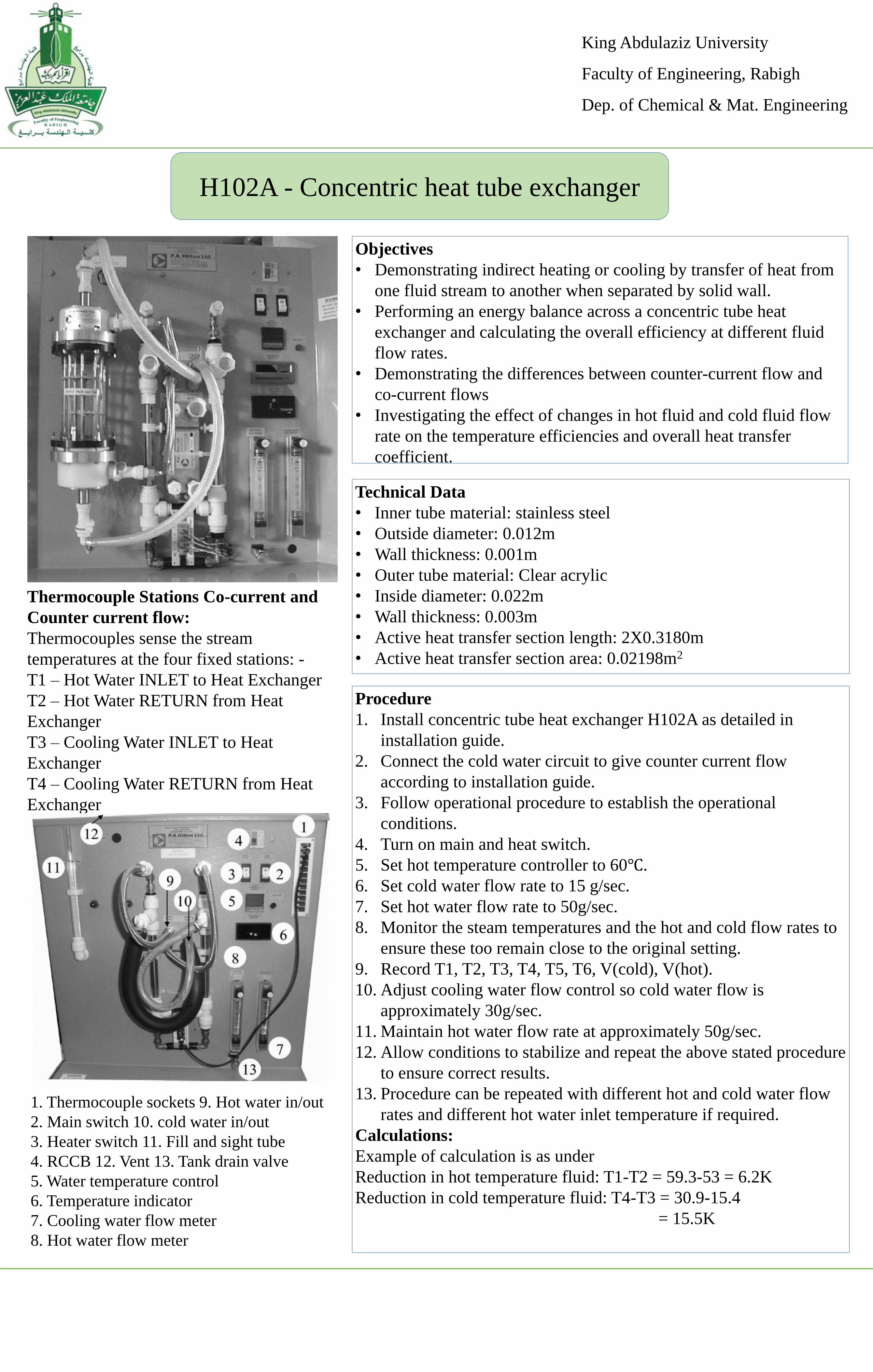
1. Thermocouple sockets 9. Hot water in/out
2. Main switch 10. cold water in/out
3. Heater switch 11. Fill and sight tube
4. RCCB 12. Vent 13. Tank drain valve
5. Water temperature control
6. Temperature indicator
7. Cooling water flow meter
8. Hot water flow meter
King Abdulaziz University
Faculty of Engineering, Rabigh
Dep. of Chemical & Mat. Engineering
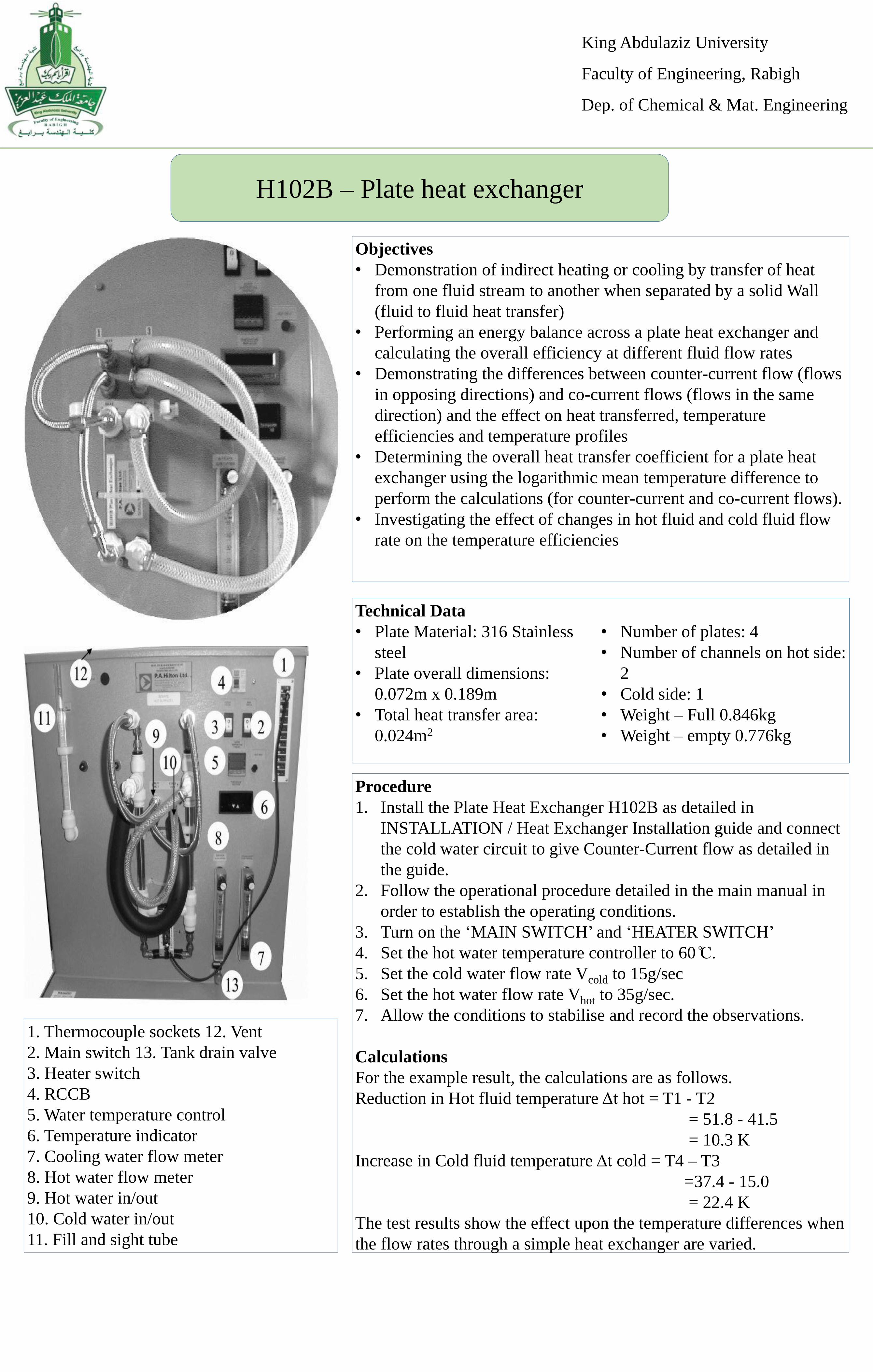
H102B – Plate heat exchanger
Technical Data
• Plate Material: 316 Stainless
steel
• Plate overall dimensions:
0.072m x 0.189m
• Total heat transfer area:
0.024m2
• Number of plates: 4
• Number of channels on hot side:
2
• Cold side: 1
• Weight – Full 0.846kg
• Weight – empty 0.776kg
1. Thermocouple sockets 12. Vent
2. Main switch 13. Tank drain valve
3. Heater switch
4. RCCB
5. Water temperature control
6. Temperature indicator
7. Cooling water flow meter
8. Hot water flow meter
9. Hot water in/out
10. Cold water in/out
11. Fill and sight tube
Objectives
• Demonstration of indirect heating or cooling by transfer of heat
from one fluid stream to another when separated by a solid Wall
(fluid to fluid heat transfer)
• Performing an energy balance across a plate heat exchanger and
calculating the overall efficiency at different fluid flow rates
• Demonstrating the differences between counter-current flow (flows
in opposing directions) and co-current flows (flows in the same
direction) and the effect on heat transferred, temperature
efficiencies and temperature profiles
• Determining the overall heat transfer coefficient for a plate heat
exchanger using the logarithmic mean temperature difference to
perform the calculations (for counter-current and co-current flows).
• Investigating the effect of changes in hot fluid and cold fluid flow
rate on the temperature efficiencies
Procedure
1. Install the Plate Heat Exchanger H102B as detailed in
INSTALLATION / Heat Exchanger Installation guide and connect
the cold water circuit to give Counter-Current flow as detailed in
the guide.
2. Follow the operational procedure detailed in the main manual in
order to establish the operating conditions.
3. Turn on the ‘MAIN SWITCH’ and ‘HEATER SWITCH’
4. Set the hot water temperature controller to 60 ̊C.
5. Set the cold water flow rate Vcold to 15g/sec
6. Set the hot water flow rate Vhot to 35g/sec.
7. Allow the conditions to stabilise and record the observations.
Calculations
For the example result, the calculations are as follows.
Reduction in Hot fluid temperature Δt hot = T1 - T2
= 51.8 - 41.5
= 10.3 K
Increase in Cold fluid temperature Δt cold = T4 – T3
=37.4 - 15.0
= 22.4 K
The test results show the effect upon the temperature differences when
the flow rates through a simple heat exchanger are varied.
King Abdulaziz University
Faculty of Engineering, Rabigh
Dep. of Chemical & Mat. Engineering
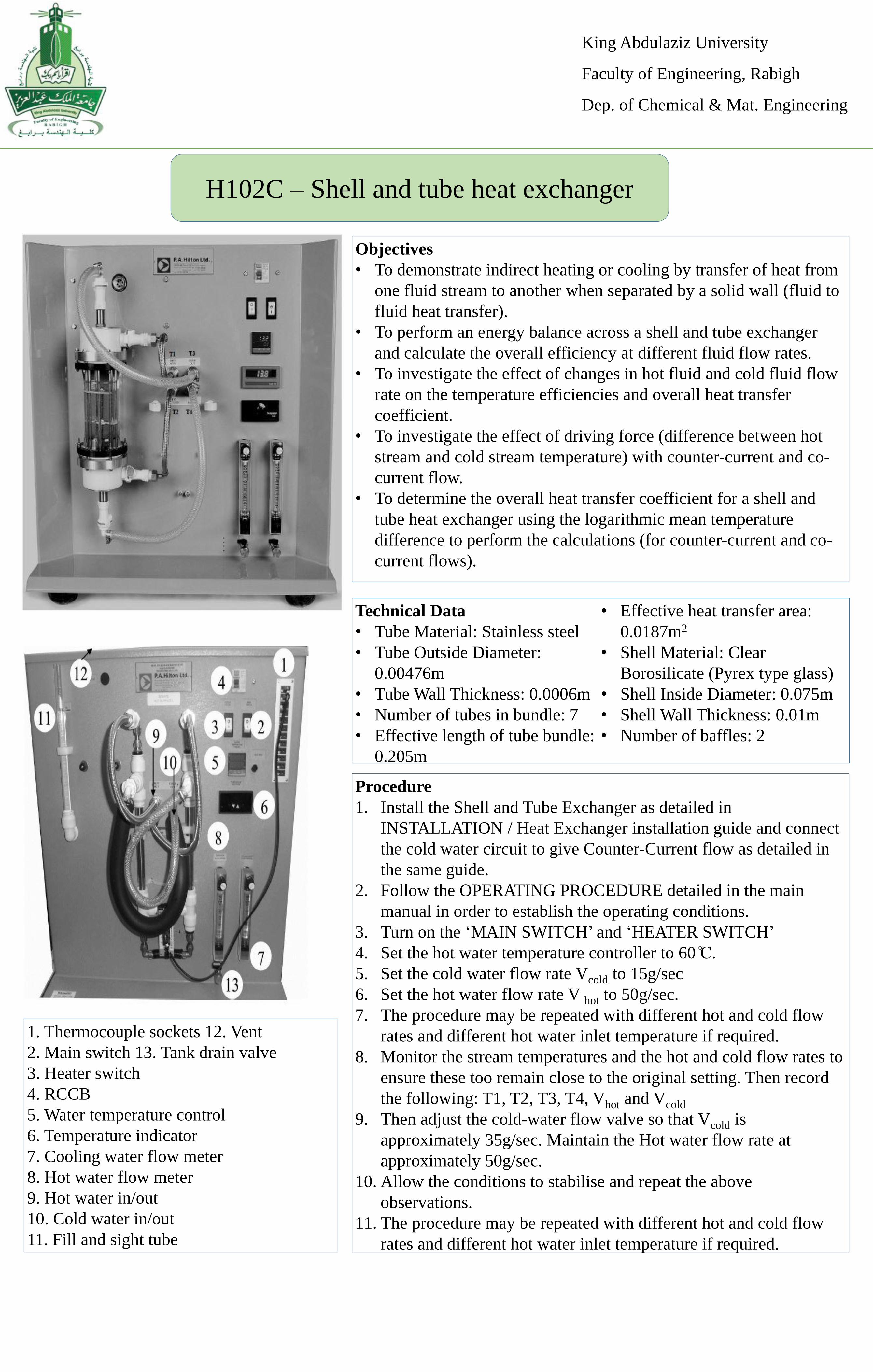
H102C – Shell and tube heat exchanger
Technical Data
• Tube Material: Stainless steel
• Tube Outside Diameter:
0.00476m
• Tube Wall Thickness: 0.0006m
• Number of tubes in bundle: 7
• Effective length of tube bundle:
0.205m
• Effective heat transfer area:
0.0187m2
• Shell Material: Clear
Borosilicate (Pyrex type glass)
• Shell Inside Diameter: 0.075m
• Shell Wall Thickness: 0.01m
• Number of baffles: 2
1. Thermocouple sockets 12. Vent
2. Main switch 13. Tank drain valve
3. Heater switch
4. RCCB
5. Water temperature control
6. Temperature indicator
7. Cooling water flow meter
8. Hot water flow meter
9. Hot water in/out
10. Cold water in/out
11. Fill and sight tube
Objectives
• To demonstrate indirect heating or cooling by transfer of heat from
one fluid stream to another when separated by a solid wall (fluid to
fluid heat transfer).
• To perform an energy balance across a shell and tube exchanger
and calculate the overall efficiency at different fluid flow rates.
• To investigate the effect of changes in hot fluid and cold fluid flow
rate on the temperature efficiencies and overall heat transfer
coefficient.
• To investigate the effect of driving force (difference between hot
stream and cold stream temperature) with counter-current and co-
current flow.
• To determine the overall heat transfer coefficient for a shell and
tube heat exchanger using the logarithmic mean temperature
difference to perform the calculations (for counter-current and co-
current flows).
Procedure
1. Install the Shell and Tube Exchanger as detailed in
INSTALLATION / Heat Exchanger installation guide and connect
the cold water circuit to give Counter-Current flow as detailed in
the same guide.
2. Follow the OPERATING PROCEDURE detailed in the main
manual in order to establish the operating conditions.
3. Turn on the ‘MAIN SWITCH’ and ‘HEATER SWITCH’
4. Set the hot water temperature controller to 60 ̊C.
5. Set the cold water flow rate Vcold to 15g/sec
6. Set the hot water flow rate V hot to 50g/sec.
7. The procedure may be repeated with different hot and cold flow
rates and different hot water inlet temperature if required.
8. Monitor the stream temperatures and the hot and cold flow rates to
ensure these too remain close to the original setting. Then record
the following: T1, T2, T3, T4, Vhot and Vcold
9. Then adjust the cold-water flow valve so that Vcold is
approximately 35g/sec. Maintain the Hot water flow rate at
approximately 50g/sec.
10. Allow the conditions to stabilise and repeat the above
observations.
11. The procedure may be repeated with different hot and cold flow
rates and different hot water inlet temperature if required.

King Abdulaziz University
Faculty of Engineering, Rabigh
Dep. of Chemical & Mat. Engineering
H102D – Jacketed vessel with coil and stirrer
Technical Data
• Vessel wall inside diameter:
0.1524m
• Vessel wall outside diameter:
0.1542m
• Coil tube outside diameter:
0.0063m
• Coil tube bore diameter:
0.0049m
• Effective length of coil tube:
1.15m
1. Thermocouple sockets 12. Vent
2. Main switch 13. Tank drain valve
3. Heater switch
4. RCCB
5. Water temperature control
6. Temperature indicator
7. Cooling water flow meter
8. Hot water flow meter
9. Hot water in/out
10. Cold water in/out
11. Fill and sight tube
Objectives
• To demonstrate indirect heating or cooling by transfer of heat from
one fluid stream to another when separated by a solid wall (fluid to
fluid heat transfer).
• To investigate the heating characteristics of a stirred vessel
containing a fixed batch of liquid when heated using hot fluid
circulating through a submerged coil.
• To investigate the heating characteristics of a stirred vessel
containing a fixed batch of liquid when heated using hot fluid
circulating through an outer jacket.
• To investigate the change in overall heat transfer coefficient and
logarithmic mean temperature difference as a batch of fluid in the
vessel changes temperature.
• To perform an energy balance, calculate the overall efficiency and
determine the overall heat transfer coefficient for a continuous flow
in a stirred vessel when heated using a submerged coil.
Procedure
1. Install the Jacketed Vessel with Coil and Stirrer H102D as detailed
in installation guide and connect the hot water circuit Using the
Outer Jacket as detailed in the same guide.
2. Adjust the overflow in the vessel to the 1-litre height.
3. Configure the Cold Water Circuit following.
4. Follow the OPERATING PROCEDURE detailed in the main
manual in order to establish the operating conditions.
5. Turn on the ‘MAIN SWITCH’ and replenish the hot circuit as the
jacket fills.
6. Turn on the ‘HEATER SWITCH’.
7. Set the hot water temperature controller to 70 ̊C.
8. Set the cold water flow rate Vcold to 8g/sec
9. Set the hot water flow rate V hot to 34g/sec.
10. Turn stirrer ON, speed to 100%.
11. Make T5 probe 15mm below surface.
CALCULATIONS
For the example result the calculations are as follows.
Reduction in Hot fluid temperature Δt hot = T1 – T2 = 70.2 – 64.2
= 6.0 K
Increase in Cold fluid temperature Δt cold = T5 – T4
=32.5 – 14.1
= 18.4 K
King Abdulaziz University
Faculty of Engineering, Rabigh
Dep. of Chemical & Mat. Engineering
H102E – Extended concentric tube
Heat exchanger
Technical Data
• Inner Tube Material: Stainless
steel
• Outside Diameter: 0.012m
• Wall Thickness: 0.001m
• Outer Tube Material: Clear
Acrylic
• Inside Diameter: 0.022m
• Wall Thickness: 0.003m
• Active Heat Transfer Section
Length 4 x 0.3180 = 0.636m
• Area 2x 0.02198= 0.04396 m2
1. Thermocouple sockets 12. Vent
2. Main switch 13. Tank drain valve
3. Heater switch
4. RCCB
5. Water temperature control
6. Temperature indicator
7. Cooling water flow meter
8. Hot water flow meter
9. Hot water in/out
10. Cold water in/out
11. Fill and sight tube
Objectives
• To demonstrate indirect heating or cooling by transfer of heat from
one fluid stream to another when separated by a solid wall (fluid to
fluid heat transfer).
• To perform an energy balance across a concentric tube heat
exchanger and calculate the overall efficiency at different fluid
flow rates.
• To determine the overall heat transfer coefficient for a concentric
tube heat exchanger using the logarithmic mean temperature
difference to perform the calculations (for counter-current and co-
current flows).
• To investigate the effect of changes in hot fluid and cold fluid flow
rate on the temperature efficiencies and overall heat transfer
coefficient.
• To investigate effect of driving force (difference b/w hot and cold
stream temperature) with counter-current and co-current flow.
Procedure
1. Install the Concentric tube Heat Exchanger as detailed in
INSTALLATION / Heat Exchanger Installation guide and connect
the cold water circuit to give Counter- Current flow as detailed in
the same section.
2. Follow the OPERATING PROCEDURE detailed in the main
manual in order to establish the operating conditions.
3. Turn on the ‘MAIN SWITCH’ and ‘HEATER SWITCH’
4. Set the hot water temperature controller to 60 ̊C.
5. Set the cold water flow rate Vcold to 10g/sec
6. Set the hot water flow rate V hot to 30 g/sec.
7. Monitor the stream temperatures and the hot and cold flow rates to
ensure these too remain close to the original setting. Then record
the following: T1, T2, T3, T4, T5, T6, T7, T8, T9, T10, Vcold and V
hot
8. Then adjust the ‘COOLING WATER FLOW CONTROL’ so that
Vcold is approximately 10g/sec.
9. Maintain the Hot water flow rate V hot at approximately 30g/sec.
10. Allow the conditions to stabilise and repeat the above
observations.
11. The procedure may be repeated with different hot and cold flow
rates and different hot water inlet temperature if required.
Co-current and Counter-current flow
Thermocouples sense the stream
temperatures at the fixed stations: -
T1 Hot stream out (on H102 Panel)
T5 Intermediate hot
T7 Intermediate hot
T10 Intermediate Hot

King Abdulaziz University
Faculty of Engineering, Rabigh
Dep. of Chemical & Mat. Engineering
H102F – Extended plate heat exchanger
Technical Data
• Plate Material: 316 Stainless
steel
• Plate overall dimensions:
0.072m x 0.189m
• Total heat transfer area 0.048m2
• Number of plates: 2x4
1. Thermocouple sockets 12. Vent
2. Main switch 13. Tank drain valve
3. Heater switch
4. RCCB
5. Water temperature control
6. Temperature indicator
7. Cooling water flow meter
8. Hot water flow meter
9. Hot water in/out
10. Cold water in/out
11. Fill and sight tube
Objectives
• To demonstrate indirect heating or cooling by transfer of heat from
one fluid stream to another when separated by a solid wall (fluid to
fluid heat transfer).
• To perform an energy balance across a plate heat exchanger and
calculate the overall efficiency at different fluid flow rates
• To demonstrate the differences between counter-current flow (flows
in opposing directions) and co-current flows and the effect on heat
transferred, temperature efficiencies and temperature profiles
through a plate heat exchanger.
• To determine the overall heat transfer coefficient for a plate heat
exchanger using the logarithmic mean temperature difference to
perform the calculations.
• To investigate the effect of changes in hot fluid and cold fluid flow
rate on the temperature efficiencies and overall heat transfer
coefficient.
Procedure
1. Install the Plate Heat Exchanger as detailed in INSTALLATION /
Heat Exchanger Installation guide and connect the cold water
circuit to give Co-Current flow as detailed in the same section.
2. Follow the OPERATING PROCEDURE detailed in the main
manual in order to establish the operating conditions.
3. Turn on the ‘MAIN SWITCH’ and ‘HEATER SWITCH’
4. Set the hot water temperature controller to 60 ̊C.
5. Set the cold water flow rate Vcold to 10g/sec
6. Set the hot water flow rate V hot to 30g/sec.
7. Allow the conditions to stabilise and record the observations.
8. The procedure may be repeated with different hot and cold flow
rates and different hot water inlet temperature if required.
CALCULATIONS
For the example result the calculations are as follows.
Reduction in Hot fluid temperature Δt hot = T1 - T2
= 60.1 – 48.5 = 11.6 K
Increase in Cold fluid temperature Δt cold = T4 – T3
=47.9 – 16.6 = 32.3 K
The test results show the effect upon the temperature differences when
the flow rates through a simple heat exchanger are varied.
Co-current and Counter-current flow
Thermocouples sense the stream
temperatures at the fixed stations: -
T1 Hot stream out (on H102 Panel)
T6 Intermediate hot
T2 Hot stream return(on H102 Panel)
T3 Cold Out (on H102 Panel)

King Abdulaziz University
Faculty of Engineering, Rabigh
Dep. of Chemical & Mat. Engineering
H102G – Water to water turbulent flow heat exchanger
Technical Data
• Core Tube Material - Copper
• External Diameter (do) =
9.5mm
• Internal Diameter (di) = 7.9mm
• Length = 3 x 350mm
• External Heat transfer area Ao =
0.031m2
• Mean Area = 0.0288m2
• Flow area Si = 49 x 10-6 m2
• Outer Tube Material - Copper
• External Diameter Do =
12.7mm
• Internal Diameter Di = 11.1mm
• Annulus flow area, So = 25.9 x
10-6 m2
1. Thermocouple sockets 12. Vent
2. Main switch 13. Tank drain valve
3. Heater switch
4. RCCB
5. Water temperature control
6. Temperature indicator
7. Cooling water flow meter
8. Hot water flow meter
9. Hot water in/out
10. Cold water in/out
11. Fill and sight tube
Objectives
• Determination of heat transfer rate, logarithmic mean temperature
difference and overall heat transfer coefficient.
• Determination of surface heat transfer coefficient inside and
outside the tube and the effect of fluid velocity on these.
• Comparison of con-current and counter-current flow in a heat
exchanger.
• Investigation of the relationship between Nusselt Number,
Reynolds Number and Prandtl Number.
Procedure
1. Set the cooling water direction for counter-current flow by
selecting the appropriate cold flow couplings as shown on manual.
2. Check that unit contains water to the correct level.
3. Fully open the hot water flow control valve.
4. Switch on the main switch and heater switch and set the water
temperature control to approximately 70℃.
5. Adjust the hot water flow rate to a convenient value – for example
maximum flow.
6. Adjust the cold water flow to approximately 10-15g s-1 .
7. Make the observations.
Calculations
Mean hot water temperature = (t7+t10)/2
Actual Flow( Litres/minute) = Indicated Flow + (T10 *0.0041) -
0.0796
Temperature Distribution
This can be found through logarithmic mean temperature difference
For the heat exchanger in the counter-current flow arrangement:
The Overall Heat Transfer Coefficient, U, may be obtained from,
Temperature distribution diagram
1. Heat Exchanger
2. Hot Water
Flowmeter
3. Hot Flow
Control
4. Hot Flow From
H102
5. Hot Flow
Return to H102
7. H102G
Securing Nuts

King Abdulaziz University
Faculty of Engineering, Rabigh
Dep. of Chemical & Mat. Engineering
H102H – Coiled concentric tube heat exchanger
Technical Data
• Inner Tube material: Copper
• Outside Diameter: 0.0214m
• Wall Thickness: 0.001m
• Outer Tube material: Steel
• Inside Diameter: 0.0194m
• Wall Thickness: 0.001m
• Active Heat Transfer Section
Length: 1.61m
• Area: 0.108m2
1. Thermocouple sockets 12. Vent
2. Main switch 13. Tank drain valve
3. Heater switch
4. RCCB
5. Water temperature control
6. Temperature indicator
7. Cooling water flow meter
8. Hot water flow meter
9. Hot water in/out
10. Cold water in/out
11. Fill and sight tube
Objectives
• To demonstrate indirect heating or cooling by transfer of heat from
one fluid stream to another when separated by a solid wall (fluid to
fluid heat transfer).
• To perform an energy balance across a concentric tube heat
exchanger and calculate the overall efficiency at different fluid
flow rates.
• To demonstrate the differences between counter-current flow (flows
in opposing directions) and co-current flows (flows in the same
direction) and the effect on heat transferred, temperature
efficiencies and temperature profiles through a concentric tube heat
exchanger.
• To determine the overall heat transfer coefficient for a concentric
tube heat exchanger using the logarithmic mean temperature
difference to perform the calculations.
• To investigate the effect of changes in hot fluid and cold fluid flow
rate on the temperature efficiencies and overall heat transfer
coefficient.
• To investigate the effect of driving force (difference between hot
stream and cold stream temperature) with counter-current and co-
current flow.
Procedure
1. Install the Coiled Concentric tube Heat Exchanger as detailed in
INSTALLATION / Heat Exchanger Installation guide and connect
the cold water circuit to give Counter-Current flow as detailed in
the same section.
2. Follow the OPERATING PROCEDURE detailed in the main
manual in order to establish the operating conditions.
3. Turn on the ‘MAIN SWITCH’ and ‘HEATER SWITCH’
4. Set the hot water temperature controller to 60 ̊C.
5. Set the cold water flow rate Vcold to 10g/sec
6. Set the hot water flow rate V hot to 30g/sec.
7. Monitor the stream temperatures and the hot and cold flow rates to
ensure these too remain close to the original setting. Then record
the following:
T1, T2, T3, T4, T5, T6, T7, T8, T9, T10, Vcold and V hot
8. Allow the conditions to stabilise and record the observations.
9. The procedure may be repeated with different hot and cold flow
rates and different hot water inlet temperature if required.
King Abdulaziz University
Faculty of Engineering, Rabigh
Dep. of Chemical & Mat. Engineering
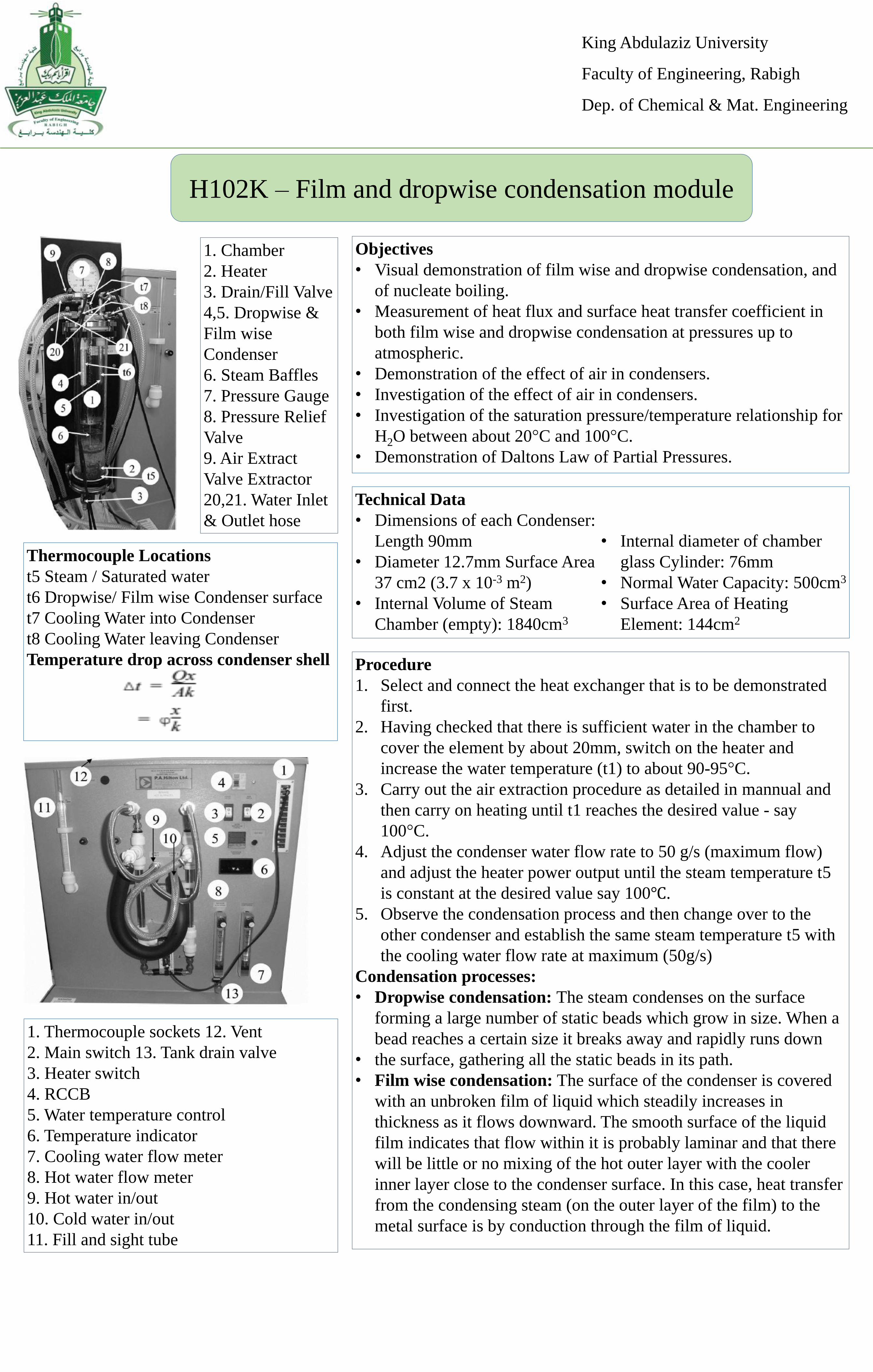
H102K – Film and dropwise condensation module
Technical Data
• Dimensions of each Condenser:
Length 90mm
• Diameter 12.7mm Surface Area
37 cm2 (3.7 x 10⁻³ m2)
• Internal Volume of Steam
Chamber (empty): 1840cm3
• Internal diameter of chamber
glass Cylinder: 76mm
• Normal Water Capacity: 500cm3
• Surface Area of Heating
Element: 144cm2
1. Thermocouple sockets 12. Vent
2. Main switch 13. Tank drain valve
3. Heater switch
4. RCCB
5. Water temperature control
6. Temperature indicator
7. Cooling water flow meter
8. Hot water flow meter
9. Hot water in/out
10. Cold water in/out
11. Fill and sight tube
Objectives
• Visual demonstration of film wise and dropwise condensation, and
of nucleate boiling.
• Measurement of heat flux and surface heat transfer coefficient in
both film wise and dropwise condensation at pressures up to
atmospheric.
• Demonstration of the effect of air in condensers.
• Investigation of the effect of air in condensers.
• Investigation of the saturation pressure/temperature relationship for
H2O between about 20°C and 100°C.
• Demonstration of Daltons Law of Partial Pressures.
Procedure
1. Select and connect the heat exchanger that is to be demonstrated
first.
2. Having checked that there is sufficient water in the chamber to
cover the element by about 20mm, switch on the heater and
increase the water temperature (t1) to about 90-95°C.
3. Carry out the air extraction procedure as detailed in mannual and
then carry on heating until t1 reaches the desired value - say
100°C.
4. Adjust the condenser water flow rate to 50 g/s (maximum flow)
and adjust the heater power output until the steam temperature t5
is constant at the desired value say 100℃.
5. Observe the condensation process and then change over to the
other condenser and establish the same steam temperature t5 with
the cooling water flow rate at maximum (50g/s)
Condensation processes:
• Dropwise condensation: The steam condenses on the surface
forming a large number of static beads which grow in size. When a
bead reaches a certain size it breaks away and rapidly runs down
• the surface, gathering all the static beads in its path.
• Film wise condensation: The surface of the condenser is covered
with an unbroken film of liquid which steadily increases in
thickness as it flows downward. The smooth surface of the liquid
film indicates that flow within it is probably laminar and that there
will be little or no mixing of the hot outer layer with the cooler
inner layer close to the condenser surface. In this case, heat transfer
from the condensing steam (on the outer layer of the film) to the
metal surface is by conduction through the film of liquid.
Thermocouple Locations
t5 Steam / Saturated water
t6 Dropwise/ Film wise Condenser surface
t7 Cooling Water into Condenser
t8 Cooling Water leaving Condenser
Temperature drop across condenser shell
1. Chamber
2. Heater
3. Drain/Fill Valve
4,5. Dropwise &
Film wise
Condenser
6. Steam Baffles
7. Pressure Gauge
8. Pressure Relief
Valve
9. Air Extract
Valve Extractor
20,21. Water Inlet
& Outlet hose

King Abdulaziz University
Faculty of Engineering, Rabigh
Dep. of Chemical & Mat. Engineering
H102M – Water to air heat exchanger
1. Thermocouple sockets 12. Vent
2. Main switch 13. Tank drain valve
3. Heater switch
4. RCCB
5. Water temperature control
6. Temperature indicator
7. Cooling water flow meter
8. Hot water flow meter
9. Hot water in/out
10. Cold water in/out
11. Fill and sight tube
Objectives
• To demonstrate indirect heating or cooling by transfer of heat from
one fluid stream to another when separated by a solid wall (fluid to
fluid heat transfer).
• To calculate the overall efficiency at different fluid flow rates
• To determine the overall heat transfer coefficient for a water to air
heat exchanger using the logarithmic mean temperature difference
to perform the calculations
Procedure
1. Install the Water to Air Heat Exchanger as detailed in
INSTALLATION manual.
2. Follow the OPERATING PROCEDURE detailed in the main
manual in order to establish the following operating conditions.
3. Turn on the ‘MAIN SWITCH’ and ‘HEATER SWITCH’
4. Set the hot water temperature controller to 70 ̊C.
5. Set the fan speed to its minimum speed.
6. Set the hot water flow rate Vhot to 50g/sec.
7. Allow the conditions to stabilise and record the observations.
Calculations
For the example result, the calculations are as follows.
Reduction in Hot fluid temperature Δt hot = T1 - T2
= 71.2 - 69.8
= 1.4 K
Increase in Cold fluid temperature Δt cold = T6 – T5
=51.7 – 19.5
= 32.2 K
Efficiency of the heat exchanger
Temperature efficiency of the hot and cold stream
Mean temperature efficiency
1. Cooling Fan
2. hot side air
thermocouple
T6
3. hot water
out coupling
4. hot water in
coupling
5. Cooling Fan
Power Supply
6. Speed
controller
7. Water to Air
Heat
Exchanger
8. Hot out
Hose
9. Hot return
Hose
10. Hot water
flow control
11.
Thermocouple
sockets
Technical data
Internal Plate Material: Aluminum
Overall dimensions 0.12m x 0.135m
Total heat transfer area 0.2025m2


