
Groundwater Vulnerability
Assessment Using a GIS-Based
Modified DRASTIC Model in
Agricultural Areas
by
Narges Gheisari
Supervisors:
Dr. Majid Sartaj, Dr. Bahram Daneshfar
Thesis submitted to the
Faculty of Graduate and Postdoctoral Studies
in partial fulfillment of the requirements for the degree of Master of Applied Science in
Civil Engineering
Department of Civil Engineering
Faculty of Engineering
University of Ottawa
© Narges Gheisari, Ottawa, Canada, 2017
Abstract
DRASTIC model is the most widely used method for aquifer vulnerability mapping
which consists of seven hydrogeological parameters. Despite of its popularity, this tech-
nique disregards the effect of regional characteristics and there is no specific validation
method to demonstrate the accuracy of this method. The main goal of this research was
developing an integrated GIS-based DRASTIC model using Depth to water, Net Recharge,
Aquifer media, Soil media, Topography, Impact of vadose zone and Hydraulic Conductiv-
ity (DRASTIC). In order to obtain a more reliable and accurate assessment, the rates
and weights of original DRASTIC were modified using Wilcoxon rank-sum non-parametric
statistical test and Single Parameter Sensitivity Analysis (SPSA). The methodology was
implemented for the Shahrekord plain in the southwestern region of Iran. Two different
sets of measured nitrate concentrations from two monitoring events were used, one for
modification and other for validation purposes. Validation nitrate values were compared
to the calculated DRASTIC index to assess the efficacy of the DRASTIC model. The vali-
dation results obtained from Pearson’s correlation and chi-square values, revealed that the
modified DRASTIC is more efficient than original DRASTIC. The modified rate/weight
DRASTIC (spline) model showed the highest correlation coefficient and chi square value as
0.88 and 72.93, respectively, compared to -0.3 and 25.2 for the original DRASTIC (spline)
model. The integrated vulnerability map showed the high risk imposed on the southeastern
part of the Shahrekord aquifer. In addition, sensitivity analysis indicated that the removal
of net recharge parameter from the modified model caused larger variation in vulnerability
index showing that this parameter has more impact on the DRASTIC vulnerability of the
aquifer. Moreover, Aquifer media (A), Topography (T) and Impact of vadose zone (I)
were found to have less effect and importance compared to other variables as expected.
Therefore, reduced modified DRASTIC model was proposed by eliminating A, T and I
parameters. Pearson’s correlation coefficient and chi-square value for the reduced model
were calculated as 0.88 and 100.38, respectively, which was found to be as reliable as full
modified DRASTIC model.
ii

Acknowledgements
Firstly, I would like to thank my supervisor, Dr. Majid Sartaj who helped me step-by-
step during my academic career.
I also want to express my special thanks of gratitude to my co-supervisor, Dr. Bahram
Daneshfar for his helpful advice and comments during my project. Thanks for the infinite
support and time.
Special thanks are due to Dr. K. Mohammadi for his sincere cooperation in providing
the data.
Lastly, I would also like to thank my beloved family, especially my husband, without
their support I would have never been able to start and finish this degree.
iii

Dedication
This is dedicated to my beloved mother.
iv

Table of Contents
List of Tables viii
List of Figures x
List of Symbols xii
1 Introduction 1
1.1 Background . . . . . . . . . . . . . . . . . . . . . . . . . . . . . . . . . . . 1
1.2 Research Objective . . . . . . . . . . . . . . . . . . . . . . . . . . . . . . . 2
1.3 Thesis Layout . . . . . . . . . . . . . . . . . . . . . . . . . . . . . . . . . . 3
2 Literature Review 4
2.1 Groundwater vulnerability . . . . . . . . . . . . . . . . . . . . . . . . . . . 4
2.2 Vulnerability mapping . . . . . . . . . . . . . . . . . . . . . . . . . . . . . 5
2.2.1 Overlay and index methods . . . . . . . . . . . . . . . . . . . . . . 6
2.2.2 Process based simulation model methods . . . . . . . . . . . . . . . 6
2.2.3 Statistical methods . . . . . . . . . . . . . . . . . . . . . . . . . . . 7
2.3 DRASTIC vulnerability mapping . . . . . . . . . . . . . . . . . . . . . . . 8
2.3.1 Depth to Water (D) . . . . . . . . . . . . . . . . . . . . . . . . . . 10
2.3.2 Net Recharge (R) . . . . . . . . . . . . . . . . . . . . . . . . . . . . 10
v

2.3.3 Aquifer Media (A) . . . . . . . . . . . . . . . . . . . . . . . . . . . 11
2.3.4 Soil Media (S) . . . . . . . . . . . . . . . . . . . . . . . . . . . . . . 11
2.3.5 Topography (T) . . . . . . . . . . . . . . . . . . . . . . . . . . . . . 11
2.3.6 Impact of Vadose Zone (I) . . . . . . . . . . . . . . . . . . . . . . . 11
2.3.7 Hydraulic Conductivity (C) . . . . . . . . . . . . . . . . . . . . . . 12
2.4 Modifications on DRASTIC . . . . . . . . . . . . . . . . . . . . . . . . . . 15
2.4.1 Weight adjustment techniques . . . . . . . . . . . . . . . . . . . . . 16
2.4.2 Rate adjustment techniques . . . . . . . . . . . . . . . . . . . . . . 20
2.5 DRASTIC Validation . . . . . . . . . . . . . . . . . . . . . . . . . . . . . . 22
2.6 Research gap . . . . . . . . . . . . . . . . . . . . . . . . . . . . . . . . . . 23
3 Material and Methods 25
3.1 Study area . . . . . . . . . . . . . . . . . . . . . . . . . . . . . . . . . . . . 25
3.2 Data and DRASTIC method . . . . . . . . . . . . . . . . . . . . . . . . . . 26
3.2.1 Depth to Water . . . . . . . . . . . . . . . . . . . . . . . . . . . . . 27
3.2.2 Net Recharge . . . . . . . . . . . . . . . . . . . . . . . . . . . . . . 29
3.2.3 Aquifer Media . . . . . . . . . . . . . . . . . . . . . . . . . . . . . . 30
3.2.4 Soil Media . . . . . . . . . . . . . . . . . . . . . . . . . . . . . . . . 31
3.2.5 Topography . . . . . . . . . . . . . . . . . . . . . . . . . . . . . . . 32
3.2.6 Impact of Vadose Zone . . . . . . . . . . . . . . . . . . . . . . . . . 33
3.2.7 Hydraulic Conductivity . . . . . . . . . . . . . . . . . . . . . . . . . 34
3.3 Nitrate measurements . . . . . . . . . . . . . . . . . . . . . . . . . . . . . 35
3.4 Validation methods . . . . . . . . . . . . . . . . . . . . . . . . . . . . . . . 36
3.4.1 Pearson’s correlation coefficient . . . . . . . . . . . . . . . . . . . . 37
3.4.2 Chi-square value . . . . . . . . . . . . . . . . . . . . . . . . . . . . 37
vi

3.5 Modification methods . . . . . . . . . . . . . . . . . . . . . . . . . . . . . . 38
3.6 Map removal sensitivity analysis . . . . . . . . . . . . . . . . . . . . . . . . 39
4 Results and Discussion 40
4.1 Original DRASTIC model . . . . . . . . . . . . . . . . . . . . . . . . . . . 40
4.2 Rate modification using nitrate concentrations . . . . . . . . . . . . . . . . 48
4.3 Weight modification using SPSA . . . . . . . . . . . . . . . . . . . . . . . . 58
4.4 Map removal sensitivity analysis . . . . . . . . . . . . . . . . . . . . . . . . 66
4.5 Discussion . . . . . . . . . . . . . . . . . . . . . . . . . . . . . . . . . . . . 72
5 Conclusion 73
5.1 Summary . . . . . . . . . . . . . . . . . . . . . . . . . . . . . . . . . . . . 73
5.2 Conclusion . . . . . . . . . . . . . . . . . . . . . . . . . . . . . . . . . . . . 74
5.3 Recommendations for future studies . . . . . . . . . . . . . . . . . . . . . . 75
References 76
vii

List of Tables
2.1 Criteria of the vulnerability assessment by using DRASTIC method [33] . . 12
2.2 Colour codes for DRASTIC Indices introduced by Aller [7] . . . . . . . . . 13
2.3 Standard DRASTIC weights and rating system [7] . . . . . . . . . . . . . 14
4.1 Correlation factors between nitrate concentrations and intrinsic DRASTIC
index . . . . . . . . . . . . . . . . . . . . . . . . . . . . . . . . . . . . . . . 43
4.2 Area cross-tabulation between DRASTIC (IDW) and nitrate (km2) . . . . 45
4.3 Chi-square values for DRASTIC (IDW) . . . . . . . . . . . . . . . . . . . . 45
4.4 Area cross-tabulation between DRASTIC (spline) and nitrate (km2) . . . . 46
4.5 Chi-square values for DRASTIC (spline) . . . . . . . . . . . . . . . . . . . 46
4.6 Standard and modified DRASTIC rates based on nitrate concentrations . . 49
4.7 Statistical summary of rates in original DRASTIC . . . . . . . . . . . . . . 50
4.8 Statistical summary of rates in modified-rates DRASTIC . . . . . . . . . . 50
4.9 Correlation factors between nitrate and modified-rates DRASTIC index . 53
4.10 Area cross-tabulation between modified-rates DRASTIC (IDW) and nitrate
(km2) . . . . . . . . . . . . . . . . . . . . . . . . . . . . . . . . . . . . . . 55
4.11 Chi-square values for modified-rates DRASTIC (IDW) . . . . . . . . . . . 55
4.12 Area cross-tabulation between modified-rates DRASTIC (spline) and nitrate
(km2) . . . . . . . . . . . . . . . . . . . . . . . . . . . . . . . . . . . . . . 56
viii

4.13 Chi-square values for modified-rates DRASTIC (spline) . . . . . . . . . . . 56
4.14 Statistics of SPSA on modified-rates DRASTIC (IDW) . . . . . . . . . . . 58
4.15 Statistics of single parameter analysis on modified-rates DRASTIC (spline) 58
4.16 Correlation factors between nitrate and MRW DRASTIC index . . . . . . 62
4.17 Area cross-tabulation between MRW DRASTIC (IDW) and nitrate (km2) . 64
4.18 Chi-square values for MRW DRASTIC (IDW) . . . . . . . . . . . . . . . . 64
4.19 Area cross-tabulation between MRW DRASTIC (spline) and nitrate (km2) 64
4.20 Chi-square values for MRW DRASTIC (spline) . . . . . . . . . . . . . . . 64
4.21 Statistics of single map removal sensitivity analysis . . . . . . . . . . . . . 67
4.22 Statistics of multiple map removal sensitivity analysis . . . . . . . . . . . . 67
4.23 Correlation between nitrate and vulnerability map obtained from single map
removal . . . . . . . . . . . . . . . . . . . . . . . . . . . . . . . . . . . . . 68
4.24 Correlation between nitrate and vulnerability map obtained from multiple
map removal . . . . . . . . . . . . . . . . . . . . . . . . . . . . . . . . . . . 68
4.25 Area cross-tabulation between reduced MRW DRASTIC map and nitrate
(km2) . . . . . . . . . . . . . . . . . . . . . . . . . . . . . . . . . . . . . . 70
4.26 Chi-square values for reduced MRW DRASTIC (spline) map . . . . . . . . 71
ix
List of Figures
2.1 Definition of DRASTIC parameters, (Source: www.frakturmedia.net) . . . 9
3.1 Location and boundry of Shahrekord plain . . . . . . . . . . . . . . . . . . 25
3.2 Distribution of measured depth points . . . . . . . . . . . . . . . . . . . . 27
3.3 Interpolated and rated depth rasters (IDW) . . . . . . . . . . . . . . . . . 28
3.4 Interpolated and rated depth rasters (spline) . . . . . . . . . . . . . . . . . 28
3.5 Net recharge map and rated raster . . . . . . . . . . . . . . . . . . . . . . 29
3.6 Aquifer map and rated raster . . . . . . . . . . . . . . . . . . . . . . . . . 30
3.7 Soil map and rated raster . . . . . . . . . . . . . . . . . . . . . . . . . . . 31
3.8 Topography map . . . . . . . . . . . . . . . . . . . . . . . . . . . . . . . . 32
3.9 Slope map and rated raster . . . . . . . . . . . . . . . . . . . . . . . . . . 33
3.10 Impact of vadose zone map and rated raster . . . . . . . . . . . . . . . . . 34
3.11 Hydraulic conductivity map and rated raster . . . . . . . . . . . . . . . . . 35
3.12 Location of nitrate samples . . . . . . . . . . . . . . . . . . . . . . . . . . 36
4.1 GIS model to calculate DRASTIC Index (based on IDW interpolation) . . 41
4.2 GIS model to calculate DRASTIC Index (based on spline interpolation) . . 41
4.3 Intrinsic vulnerability map and area percentages (IDW) . . . . . . . . . . . 42
4.4 Intrinsic vulnerability map and area percentages (spline) . . . . . . . . . . 42
x

4.5 Correlation between intrinsic DRASTIC index (IDW) and nitrate . . . . . 43
4.6 Correlation between intrinsic DRASTIC index (spline) and nitrate . . . . 44
4.7 Interpolated nitrate map . . . . . . . . . . . . . . . . . . . . . . . . . . . . 45
4.8 Nitrate validation samples on DRASTIC (IDW) map . . . . . . . . . . . . 47
4.9 Nitrate validation samples on DRASTIC (spline) map . . . . . . . . . . . 47
4.10 Modified-rates DRASTIC (IDW) map and area percentages . . . . . . . . 51
4.11 Modified-rates DRASTIC (spline) map and area percentages . . . . . . . . 52
4.12 Correlation between modified-rates DRASTIC index (IDW) and nitrate . 54
4.13 Correlation between modified-rates DRASTIC index (spline) and nitrate . 54
4.14 Nitrate validation samples on modified-rates DRASTIC (IDW) map . . . 57
4.15 Nitrate validation samples on modified-rates DRASTIC (spline) map . . . 57
4.16 Comparison of weights of parameters before and after modification (IDW) 59
4.17 Comparison of weights of parameters before and after modification (spline) 59
4.18 MRW DRASTIC map and area percentages (IDW) . . . . . . . . . . . . . 61
4.19 MRW DRASTIC map and area percentages (spline) . . . . . . . . . . . . . 61
4.20 Correlation between MRW DRASTIC index and nitrate (IDW) . . . . . . 62
4.21 Correlation between MRW DRASTIC index and nitrate (spline) . . . . . . 63
4.22 Nitrate validation samples on MRW DRASTIC (IDW) map . . . . . . . . 65
4.23 Nitrate validation samples on MRW DRASTIC (spline) map . . . . . . . . 66
4.24 Reduced MRW DRASTIC (spline) map . . . . . . . . . . . . . . . . . . . . 69
4.25 Comparison between full and reduced MRW DRASTIC (spline) maps . . 69
4.26 Correlation between reduced MRW DRASTIC (spline) index and nitrate . 70
xi

List of Symbols
A: Aquifer media
AHP: Analytical Hierarchy process
b: Thickness of aquifer (m)
C: Hydraulic conductivity
CI: Consistency index
D: Depth to water
DI: DRASTIC Index
EPA: Environmental Protection Agency
FR: Frequency ratio
GIS: Geographic Information System
H: High
k: Hydraulic conductivity (m/d)
I: Impact of vadose zone
IDW: Inverse Distance Weighting
L: Low
M: Moderate
MH: Moderate High
ML: Moderate Low
MRW DRASTIC: Modified rate and weight DRASTIC
n: Number of layers
P: Probability of contaminant concentration
r: Pearson’s correlation coefficient
R: Net recharge
S: Sensitivity index
S: Soil media
SPSA: Single Parameter Sensitivity Analysis
T: Transmisivity (m2/d)
T: Topography
V: Overall vulnerability index
V: Unperturbed vulnerability index
V’: Perturbed vulnerability index
VH: Very High
VL: Very Low
W: Weight of parameter
WoE: Weights of evidence
λmax: Maximum consistency vectorχ2: Chi-square value
xii

Chapter 1
Introduction
1.1 Background
Groundwater could be considered as one of the most important natural resources in order
to develop a society, especially in arid and semi-arid regions. In many countries with
limited sources of water, groundwater is the only water supply. Groundwater accounts for
about 90% of the freshwater supply available for mankind and provides roughly one third of
the worlds drinking water [11]. Population growth and severe demands on these resources
can result in shortage of water in future years. Despite of the significance of groundwater
as the most important component of sustainable development, it has not received enough
attention when it comes to its protection against pollution. This invaluable resource has
been at risk of depletion and pollution [53], therefore, it seems vital to protect it from
pollution and deterioration. If an aquifer gets polluted, then remediation would be difficult,
costly and at times impossible [12, 52]. During last decades, intense agriculture activities
and fertilizer application have resulted in groundwater contamination, which has become
a critical issue. In addition to agricultural activities, release of municipal and industrial
wastes have caused an increase in contaminants in subsurface environment.
Contamination of groundwater can result in poor water quality, health problems and
high costs of treatment. Assessment of aquifer vulnerability is an important step in order to
plan and implement any plan for protection of groundwater resources against contaminants
1

such as nitrate. In recent years, modeling groundwater contamination and knowledge of
where pollution may occur has received considerable attention and environmental managers
and responsible authorities have been interested in evaluating groundwater vulnerability
to pollution and likelihood of contaminants concentration exceeding acceptable levels [83].
Many approaches have been developed to assess aquifer vulnerability; overlay and index
based techniques [7], process based simulation techniques [51] and statistical techniques
[21]. DRASTIC is one of the most frequently used models for vulnerability assessment of
groundwater resources. It is an overlay and index model introduced to produce vulnera-
bility scores for different locations by combining several hydrogeological layers. Despite its
popularity, this technique disregards the type of pollution and the effect of regional charac-
teristics. Also, there is not a specific validation method to demonstrate the accuracy of this
method. Thus, this model could be modified according to specifications of pollutants and
aquifers. Nitrate contamination of aquifers is a significant problem in many agricultural
areas [11]. Nitrate, the primary form of nitrogen, is not in groundwater system naturally
but it can be one of the predominant contaminants associated with agricultural activities.
It has high solubility and mobility and can easily reach groundwater. Thus it could be a
serious threat to groundwater resources. Therefore, measured nitrate concentrations from
monitoring wells can be used to associate and correlate the contaminant in the aquifer to
the vulnerability index.
1.2 Research Objective
The main objective of this research was to determine the feasibility of DRASTIC model
for assessment of aquifer vulnerability in agricultural areas by verifying the model output
vs field measurements for nitrate concentration in groundwater. It was also intended to
modify this model within the study area by modifying the weights and rates used in the
original DRASTIC model. Therefore, a data driven component was added to DRASTIC
model to introduce a hybrid model for vulnerability assessment. Also, the possibility
of modifying DRASTIC model by eliminating some of the parameters which have less
impact on outcome was investigated. This could result in a more simple model with less
2

number of parameters and as a results less amount of required input data to enhance its
performance in predicting the vulnerability of groundwater resources. DRASTIC model
uses seven parameters, mainly characteristics of the aquifer, to assess the vulnerability or
potential for groundwater contamination. These include: Depth to water, net Recharge,
Aquifer media, Soil media, Topography, Impact of vadose zone and hydraulic Conductivity
(DRASTIC). It is an empirical model introduced by Environmental Protection Agency (US
EPA, 1985). Since DRASTIC model disregards the effects of regional characteristics and
particular type of contaminants, it must be modified based on specifications of aquifer and
pollutant. In order to obtain a more accurate and reliable vulnerability assessment, the
rates and weights of DRASTIC parameters were calibrated. Therefore, rates were modified
using nitrate concentrations representing the extent of pollution in the groundwater system.
The relative importance of the DRASTIC method parameters through Single Parameter
Sensitivity Analysis (SPSA) was evaluated. Moreover, variation index was measured using
map removal sensitivity analysis, to identify the sensitivity of vulnerability map towards
removing one or more maps. Lastly, an additional objective was to implement the combined
use of DRASTIC and Geographical Information System (GIS) as an effective method for
groundwater vulnerability mapping and water resource management.
1.3 Thesis Layout
This dissertation contains five chapters. Chapter 1 is introduction, comprising the back-
ground, objectives, and layout of the thesis. In chapter 2, a literature review on the
groundwater vulnerability mapping and the available techniques in order to evaluate vul-
nerability is presented. Chapter 3 is the materials and methodology used in this study.
Results and discussion are provided in chapter 4. A summary of the conclusions and the
suggested future work is discussed in Chapter 5.
3

Chapter 2
Literature Review
2.1 Groundwater vulnerability
In recent years, modeling of large scale groundwater contamination and the need for strate-
gic planning for aquifers protection have received considerable attention [8, 9]. Ground-
water contaminants include inorganic pollutants such as arsenic, aluminum, lead, mercury,
fluoride, iron, and nitrate and man made organic pollutants such as pesticides, plasticizes,
and chlorinated solvents [40]. Accordingly, it is essential to monitor and evaluate ground-
water quality especially in regions where groundwater is the main source for drinking water.
The concept of groundwater vulnerability to contamination was developed by Mar-
gat [62] which provides a better understanding of ground water sensitivity against pollu-
tion with respect to geological, hydrological and meteorological conditions. Because many
aquifers are permeable, shallow, unconfined and highly susceptible to contamination so it
could be considered as a powerful measure in planning for protection of aquifers. Ground-
water vulnerability is a relative, dimensionless and non measurable feature which relies on
geological and hydrogeological properties of an aquifer [10, 35]. Assessment of vulnerabil-
ity gives researchers the opportunity to evaluate the risk and sensitivity of an aquifer to
get contaminated and constitutes an essential component of management options to pre-
serve the groundwater quality [99]. Vulnerability assessment must be objective, scientific
and based on accurate evidence [68]. As aquifer vulnerability assessment is an inexact
4
estimation [56], it is considered as a tool for predicting potential contaminants, but not
necessarily for appropriate level of pollution [81].
It is now more than forty years since the vulnerability concept was proposed, but there
is not a perfect and complete definition of aquifer vulnerability. Foster in 1987 defined
vulnerability as ”the intrinsic characteristics which determine the sensitivity of various
parts of an aquifer to being adversely affected by an imposed contamination load” [37].
The best way to map aquifer vulnerability is the evaluation by a three dimensional model
which takes into account all characteristics of aquifer and its variability with space and
time. In practice, due to amount and quality of available data, budget and time constraints,
the output of vulnerability assessment would be a two dimensional map where at each point
different properties of aquifer be integrated to predict the potential pollution.
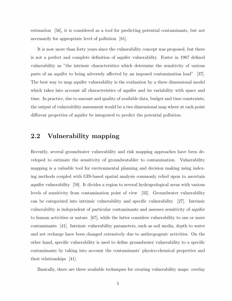
2.2 Vulnerability mapping
Recently, several groundwater vulnerability and risk mapping approaches have been de-
veloped to estimate the sensitivity of groundwatabler to contamination. Vulnerability
mapping is a valuable tool for environmental planning and decision making using index-
ing methods coupled with GIS-based spatial analysis commonly relied upon to ascertain
aquifer vulnerability [59]. It divides a region to several hydrogeological areas with various
levels of sensitivity from contamination point of view [32]. Groundwater vulnerability
can be categorized into intrinsic vulnerability and specific vulnerability [27]. Intrinsic
vulnerability is independent of particular contaminants and assesses sensitivity of aquifer
to human activities or nature [67], while the latter considers vulnerability to one or more
contaminants [41]. Intrinsic vulnerability parameters, such as soil media, depth to water
and net recharge have been changed extensively due to anthropogenic activities. On the
other hand, specific vulnerability is used to define groundwater vulnerability to a specific
contaminants by taking into account the contaminants’ physico-chemical properties and
their relationships [41].
Basically, there are three available techniques for creating vulnerability maps: overlay
5

and index based techniques [7, 25, 28, 37, 61]; process based simulation techniques [39, 50,
51, 85, 95]; and statistical techniques [21, 64, 93, 96]. Although, with respect to particular
factors and under specific circumstances they have strengths and weaknesses.
2.2.1 Overlay and index methods
The overlay and index methods are the most widespread techniques in vulnerability map-
ping due to low requirement on field data. These methods include a set of subjective
ratings and weights which consider different physical and hydrogeological factors to con-
trol movement of pollutants through the unsaturated zone till they reach the watertable
and spread [7]. Overlay and index methods are often preferred because of availability
of the required data and relatively simple procedures. Actually, these methods include
important parameters in groundwater vulnerability evaluation without attempting to fully
describe the processes that lead to contamination. Despite of simplicity and convenience,
there are some disadvantages in vulnerability mapping using overlay and index methods.
Firstly, this system assumes a linear relationship between vulnerability and parameters
while some studies have shown non-linear superposition [76]. Secondly, all weights and
rates are subject to expert judgment which introduce a subjective effect into result [38].
Thirdly, the value for ratings are discretized that could introduce additional error. There
are many index systems for groundwater vulnerability mapping, including SINTACS [26],
GOD [37], AVI [92], PI [42], GLA [44] and DRASTIC [7] which is the most widely used
technique for vulnerability mapping.
2.2.2 Process based simulation model methods
Process-based methods predict contaminant flow and transport using simulation models
and the required data for this method must be obtained by indirect techniques [16].
These methods may use the advective-dispersive solute transport approach along with
different chemical reaction models that can describe the dynamics a pollutant may un-
dergo. Process-based simulation models require analytical or numerical solutions to math-
6

ematical equations that present coupled processes affecting contaminant transport. Meth-
ods in this class range from indices based on simple transport models to analytical so-
lutions for one-dimensional transport of contaminants through the unsaturated zone to
coupled, unsaturated-saturated, multiple-phase, two- or three-dimensional models. These
approaches are different from others in that many of them attempt to predict contaminant
transport in both space and time [46]. Meeks and Dean (1990) used a one-dimensional
advection-dispersion transport model to develop a leaching potential index, which sim-
ulates vertical movement through a soil to the watertable [66]. Soutter and Pannatier
(1996) expressed groundwater vulnerability as the ratio between the cumulative pesticide
flux reaching mean watertable depth and the total quantity of pesticide applied [91].
Process-based models such as Visual ModFlow provide excellent tools to predict water
flow and pollutant transport under specific hydrogeologic conditions in the unsaturated
zone, in particular those that are highly layered (heterogeneous), and for chemical process
that undergo multiple chemical processes or chemical reactions [46]. The most important
disadvantage of this method is that they need a large volume of input data with considerable
calculation power and difficulties in calibration process [46].
2.2.3 Statistical methods
Statistical methods using different degrees of complexities in statistics, identify parameters
which are affecting groundwater contamination and they are suitable for specific regions
[14]. They produce a correlation between explanatory parameters and contaminant con-
centration [65]. These methods have been used in the evaluation of vulnerability using
probability models and results are expressed as probabilities. In general, these models in-
clude multiple independent variables and use a contaminant concentration or a probability
of contamination as the dependent variable [46]. Teso (1996) proposed a logistic regres-
sion model containing independent variables related to the soil texture. The dependent
variable was defined as the contamination status of soil sections (uncontaminated vs. con-
taminated) and groundwater vulnerability was thus assessed through the estimation of a
sections probability of its containing a contaminated well [93]. Worrall and Kolpin (2004)
7

introduced a logistic regression model of groundwater contamination that brings together
variation in chemical properties with land use, soil and aquifer characteristics.
Undoubtedly, simulation and statistical techniques provide more accurate information
for water resource managers by relying on professional judgments, hence, they are preferred
over the overlay index methods in the event required input data are available [36]. More
or less, all vulnerability models consider similar factors for predicting contamination, the
only difference is the type of approach they apply for integration [57].
2.3 DRASTIC vulnerability mapping
DRASTIC is one of the most well-known and widely used parametric vulnerability mapping
techniques. It was developed through an EPA (Environmental Protection Agency) project
in the United States with the purpose of helping managers, planners and administrators.
DRASTIC can be used in extensive regions due to low cost of application and easy to
collect data requirements [7]. According to Panagopoulos (2006) ”the selection of many
parameters and their interrelationship decreases the probability of ignoring some important
parameters, restricts the effect of an incidental error in the calculation of a parameter and
so enhances the statistical accuracy of the model” [82]. This overlay index vulnerability
method is based on physical and hydrogeological characteristics of aquifer to assess intrinsic
vulnerability [4, 7]. DRASTIC method is easy to implement and many researchers have
applied it for evaluating groundwater vulnerability around the world. It has been applied in
many regions to evaluate groundwater vulnerability, for instance in Iran [1, 68, 75], Jordan
[5], Europe [23, 31, 72], United states [84] and Africa [79]. This methodology uses seven
hydrogeological parameters which considering various parameters decreases the probability
of misjudging and enhances the reliability of vulnerability index [86]. DRASTIC acronym
stands for quantitative and categorical variables including: Depth of water, net Recharge,
Aquifer media, Soil media, Topography, Impact of vadose zone and hydraulic Conductivity.
Figure 2.1 displays the schematic diagram of DRASTIC parameters.
DRASTIC model is according to Delphi approach accomplished by a committee of
8

Figure 2.1: Definition of DRASTIC parameters, (Source: www.frakturmedia.net)
experts so the weight and rates of parameters may not be changed. Groundwater vulner-
ability mapping using DRASTIC assumes some points which are [7]:
� The contaminant is released at the earth’s surface (use of fertilizers, burning of coal
and leaching of metals from coal-ash tailings etc.).
� The contaminant flushes into the groundwater through precipitation.
� The contaminant moves with the velocity of water.
� The concerned area should be 100 acres (0.4 km2) or larger.
The original DRASTIC index (DI) was calculated by applying a linear combination of all
parameters as demonstrated by Eq. 2.1:
DI = DW .DR +RW .RR + AW .AR + SW .SR + TW .TR + IW .IR + CW .CR (2.1)
9
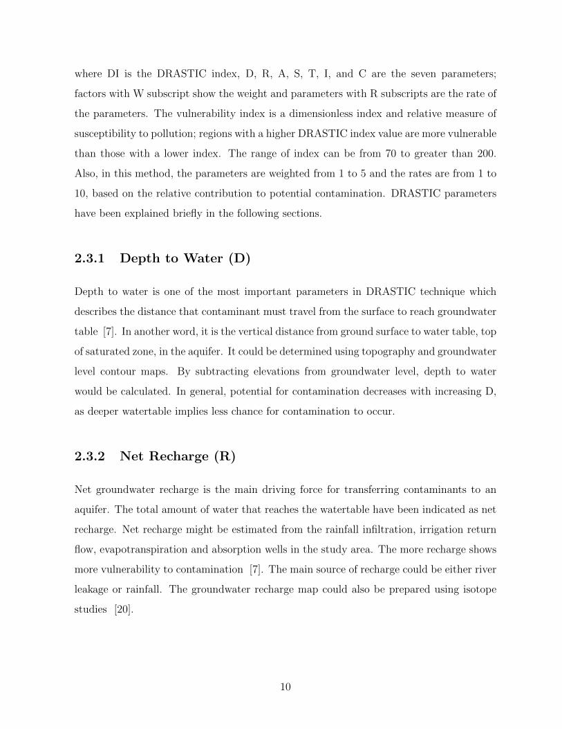
where DI is the DRASTIC index, D, R, A, S, T, I, and C are the seven parameters;
factors with W subscript show the weight and parameters with R subscripts are the rate of
the parameters. The vulnerability index is a dimensionless index and relative measure of
susceptibility to pollution; regions with a higher DRASTIC index value are more vulnerable
than those with a lower index. The range of index can be from 70 to greater than 200.
Also, in this method, the parameters are weighted from 1 to 5 and the rates are from 1 to
10, based on the relative contribution to potential contamination. DRASTIC parameters
have been explained briefly in the following sections.
2.3.1 Depth to Water (D)
Depth to water is one of the most important parameters in DRASTIC technique which
describes the distance that contaminant must travel from the surface to reach groundwater
table [7]. In another word, it is the vertical distance from ground surface to water table, top
of saturated zone, in the aquifer. It could be determined using topography and groundwater
level contour maps. By subtracting elevations from groundwater level, depth to water
would be calculated. In general, potential for contamination decreases with increasing D,
as deeper watertable implies less chance for contamination to occur.
2.3.2 Net Recharge (R)
Net groundwater recharge is the main driving force for transferring contaminants to an
aquifer. The total amount of water that reaches the watertable have been indicated as net
recharge. Net recharge might be estimated from the rainfall infiltration, irrigation return
flow, evapotranspiration and absorption wells in the study area. The more recharge shows
more vulnerability to contamination [7]. The main source of recharge could be either river
leakage or rainfall. The groundwater recharge map could also be prepared using isotope
studies [20].
10

2.3.3 Aquifer Media (A)
Aller (1987) defined aquifer as a rock formation which yield sufficient amount of water for
use. Aquifer media refers to consolidated and unconsolidated rocks (such as sand, gravel or
limestone) which serves as an aquifer [7]. This parameter is essential to control the route,
path length and movement of contaminants. In general terms, large sediment size, higher
permeability and lower attenuation capacity can result more vulnerability to pollution.
Aquifer media map could be prepared using geological information.
2.3.4 Soil Media (S)
The soil media represents the top weathered portion of unsaturated zone with significant
biological activities [7]. It is the top part of vadose zone and its characteristics are important
in potential pollution while by increasing the depth of soil, infiltration will be decreased.
Generally, soil map can represent infiltration rates of pollutants. There are some effective
factors that determine the potential pollution of soil comprising the type of clay, the grain
size and shrink potential of clay. Indeed, less amount of clay, less shrinkage potential and
smaller grain size indicate lower vulnerability of aquifer.
2.3.5 Topography (T)
Topography refers to slope of land surface and it controls the runoff of contaminants.
This factor indicates the probability that contaminant run off or remain on the ground to
infiltrate. Therefore, steep slopes increase runoff which contains contaminants and lower
chance of infiltration [6]. Digital Elevation Model could be used to prepare topography
maps and slope is calculated by GIS tools.
2.3.6 Impact of Vadose Zone (I)
The vadose zone also termed unsaturated zone, extends from the top of the ground surface
to watertable at which groundwater is at atmospheric pressure. Vertical movement of water
11

in vadose zone is important for pollution transport. The characteristic of unsaturated zone
can determine attenuation properties of the media above watertable. A vadose zone map
is also prepared using sub-surface geology and lithology characteristics of drilling logs.
2.3.7 Hydraulic Conductivity (C)
The ability of an aquifer to transmit water and contaminants is defined as hydraulic con-
ductivity. The results of pumping test and lithology are used for creating a hydraulic
conductivity distribution map. Regions with higher hydraulic conductivity indicate more
contaminant transmission and distribution. It is also controlled by pore spaces and frac-
tures within aquifer. The equation k=T/b might be used to calculate hydraulic conduc-
tivity of aquifer where the hydraulic conductivity of the aquifer is denoted by k (m/d),
transmissivity is denoted by T (m2/d) and the thickness of the aquifer is denoted by b (m).
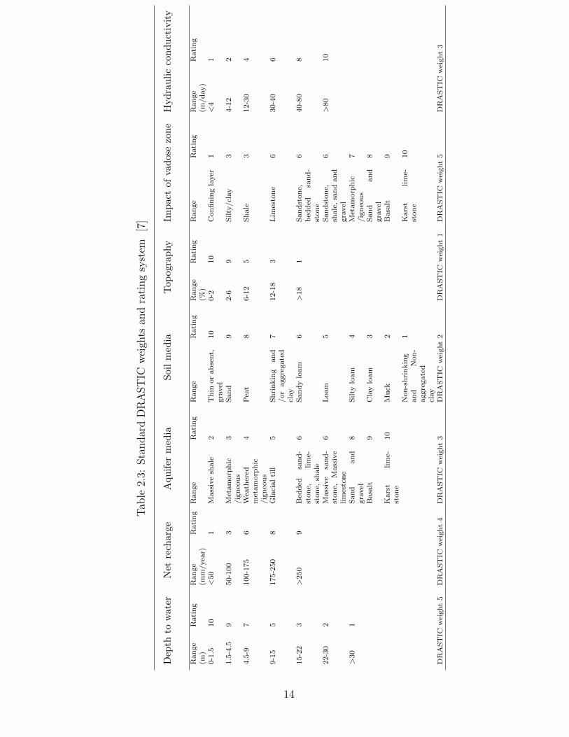
As it was mentioned, DRASTIC approach allocates specific weight and rate for each
parameter in order to calculate aquifer vulnerability index. Tables 2.1 and 2.2 present
the ranges and colour codes for DRASTIC indices. All the recommended rates and weights
are also shown in Table 2.3.
Table 2.1: Criteria of the vulnerability assessment by using DRASTIC method [33]
Class vulnerability Low Average High Very High
Calculated index value <101 101-140 141-200 >200
12

Table 2.2: Colour codes for DRASTIC Indices introduced by Aller [7]
Calculated index value Colour
less than 79 Violet
79-99 Indigo
100-119 Blue
120-139 Dark green
140-159 Light green
160-179 Yellow
180-199 Orange
200 and above Red
13
Tab
le2.
3:Sta
ndar
dD
RA
ST
ICw
eigh
tsan
dra
ting
syst
em[7
]
Dep
thto
wat
erN
etre
char
geA
qu
ifer
med
iaS
oil
med
iaT
opog
rap
hy
Imp
act
ofva
dos
ezo
ne
Hyd
rau
lic
cond
uct
ivit
y
Ran
ge
(m)
Rati
ng
Ran
ge
(mm
/yea
r)R
ati
ng
Ran
ge
Rati
ng
Ran
ge
Rati
ng
Ran
ge
(%)
Rati
ng
Ran
ge
Rati
ng
Ran
ge
(m/d
ay)
Rati
ng
0-1
.510
<50
1M
ass
ive
shale
2T
hin
or
ab
sent,
gra
vel
10
0-2
10
Con
fin
ing
layer
1<
41
1.5
-4.5
950-1
00
3M
etam
orp
hic
/ig
neo
us
3S
an
d9
2-6
9S
ilty
/cl
ay
34-1
22
4.5
-97
100-1
75
6W
eath
ered
met
am
orp
hic
/ig
neo
us
4P
eat
86-1
25
Sh
ale
312-3
04
9-1
55
175-2
50
8G
laci
al
till
5S
hri
nkin
gand
/or
aggre
gate
dcl
ay
712-1
83
Lim
esto
ne
630-4
06
15-2
23
>250
9B
edd
edsa
nd
-st
on
e,lim
e-st
on
e,sh
ale
6S
an
dy
loam
6>
18
1S
an
dst
on
e,b
edd
edsa
nd
-st
on
e
640-8
08
22-3
02
Mass
ive
san
d-
ston
e,M
ass
ive
lim
esto
ne
6L
oam
5S
an
dst
on
e,sh
ale
,sa
nd
an
dgra
vel
6>
80
10
>30
1S
an
dan
dgra
vel
8S
ilty
loam
4M
etam
orp
hic
/ig
neo
us
7
Basa
lt9
Cla
ylo
am
3S
an
dan
dgra
vel
8
Kars
tlim
e-st
on
e10
Mu
ck2
Basa
lt9
Non
-sh
rin
kin
gan
dN
on
-aggre
gate
dcl
ay
1K
ars
tlim
e-st
on
e10
DR
AS
TIC
wei
ght
5D
RA
ST
ICw
eight
4D
RA
ST
ICw
eight
3D
RA
ST
ICw
eight
2D
RA
ST
ICw
eight
1D
RA
ST
ICw
eight
5D
RA
ST
ICw
eight
3
14

2.4 Modifications on DRASTIC
Despite of simplicity and popularity, there are some weaknesses in vulnerability mapping
using DRASTIC technique. The main drawback is its subjectivity and doubts regarding
the selection of specific parameters and exclusion of others [82]. In fact, DRASTIC has
been criticized on the following points:
� It disregards the effect of regional characteristics by assigning uniform rates and
weights to parameters.
� This technique does not use a standard validation method.
� Parameters were selected based on qualitative judgment and not quantitative studies.
Therefore, many researchers have attempted to modify DRASTIC model in order to achieve
a more accurate vulnerability assessment. For instance, some researchers correlated DRAS-
TIC index with chemical or contaminant parameters but in many cases they found low
correlation. McLay (2001) suggested that models such as DRASTIC with a land manage-
ment index included, may be useful for predicting areas for more intensive monitoring of
groundwater. It was also emphasized that there is a greater need to test the link between
measurements of nitrate leaching from a variety of land use activities with measurements
of groundwater nitrate concentrations below these activities [65]. Panagopoulos (2006)
incorporated the application of simple statistical and geostatistical techniques for the revi-
sion of the factor weightings and ratings of all the DRASTIC parameters in a GIS environ-
ment. For this modification hydraulic conductivity and soil media were eliminated from the
DRASTIC equation, while land use was considered as an additional DRASTIC parameter.
The correlation coefficient between groundwater vulnerability index and nitrate concen-
trations was considerably improved and rose by 33% compared to the standard method
[82]. Leone (2009) reported the DRASTIC scores related to groundwater nitrate content.
Scores were distributed in two different groups: lower vulnerability (between 60 and 80)
with no nitrate content and higher vulnerability (between 110 and 155) with great various
nitrate contents from near to 0 to over 160 mg/L [55]. One of the important reasons for
15

this dissimilarity is the need to perform interpolation of sparse field data, which involves
error in interpolation. Hence, the results from DRASTIC should be modified according to
specification of region and contaminant. For this purpose, numerous techniques have been
suggested to develop and modify DRASTIC algorithm.
2.4.1 Weight adjustment techniques
In many studies, DRASTIC is subject to modifications, especially for the factor weights,
to meet the specifications of the study area. The weight of parameters in DRASTIC could
be modified by using different methods that have been discussed in the following sections:
2.4.1.1 Sensitivity Analysis
DRASTIC is implemented using seven hydrogeological layers which some researchers be-
lieve it could mitigate the error and uncertainties on the final vulnerability assessment
[86]. Other researchers emphasize that more appropriate vulnerability assessment could be
obtained by integrating lower number of parameters [17]. Meanwhile, sensitivity analysis
could be performed to evaluate the required layers in DRASTIC vulnerability mapping.
There are two sensitivity analysis; The map removal sensitivity analysis introduced by
Lodwick et al. [58] and the Single Parameter Sensitivity Analysis (SPSA) introduced by
Napalitano and Fabbri [72]. The map removal sensitivity analysis determines the sensi-
tivity of vulnerability map to removing one or more layers and is computed by the Eq.
2.2:
S = (|V/N − V ′/n|/V )× 100 (2.2)
where S is the sensitivity index, V is unperturbed vulnerability index, V´is perturbed
vulnerability index, and N and n are the number of data layers used to compute V and
V´. The actual vulnerability index obtained using all seven parameters is considered as an
unperturbed vulnerability while the vulnerability computed using a lower number of data
layers is considered as a perturbed one [14].
The SPSA examines the significance of each layer in vulnerability index. It is also
16

possible to compare the theoretical and effective weight of each parameter. The effective
weight of each parameter is computed using the Eq. 2.3:
W = ((Pr.Pw)÷ V )× 100 (2.3)
where W refers to the effective weight of each parameter, Pr and Pw are the rating value
and the weight of each parameter, respectively, and V is the overall vulnerability index
[14].
In recent years, many researchers have used sensitivity analysis to modify the weight
values recommended in DRASTIC method in order to increase the accuracy and reliability
of assessment [2, 18, 49, 73, 75, 79, 87, 90]. Neshat (2014) modified the weights of DRASTIC
using SPSA and concluded that modified DRASTIC model performed more efficiently
than the traditional method for non-point source pollution. DRASTIC was applied for
Kerman plain in Iran and the regression coefficients showed that the relationship between
the vulnerability index and the nitrate concentration was 82 % after modification compared
to 44 % before modification [75]. Pacheco (2015) applied sensitivity analysis for 26 aquifer
systems in Portugal with the modified DRASTIC approach. This resulted in vulnerability
indices that on average were 20% lower the original DRASTIC values [80]. Ouedraogo
(2016) applied sensitivity analysis in aquifer systems in Africa and indicated that the
removal of the impact of vadose zone, the depth to water, the hydraulic conductivity and the
net recharge caused a large variation in the mapped vulnerability. He also illustrated that
the nitrate concentration data are positively related to the intrinsic vulnerability index with
0.94 as correlation coefficient [79]. Moreover, Abdullah (2016) applied sensitivity analysis
in Halabja Saidsadiq Basin located in the northeastern part of Iraq and demonstrated
that the modified DRASTIC was dramatically superior to the standard model. Pearson
correlation factor showed that there is a good relation between the modified DRASTIC
index and nitrate concentration which were 0.69, 0.57, and 0.72 for modified rate (using
nitrate concentration), weight (sensitivity analysis), and combined rate-weight methods,
respectively [2].
17

2.4.1.2 Logistic regression
In this method, contaminant of concern as a dependent variable has to be allocated as
binary, coded as 0 for regions where the concentration is below a pre-defined threshold and
as 1 elsewhere. Then, the equation obtained from Logistic Regression will be written as
Eq. 2.4:
P =ebo + eb1x1 + ....+ ebpxp
1 + ebo + eb1x1 + ....+ ebpxp(2.4)
where P is the probability of contaminant concentration being higher than the given thresh-
old, Xj is the rating of factor j and the bj constants are adjustment coefficients. These
coefficients are optimized by the Maximum Likelihood Estimation during a run of Logistic
Regression [80]. Many researchers have used logistic regression in order to correlate nitrate
concentration with hydrogeological factors [77]. Mair and El-Kadi (2013) used logistic re-
gression modeling for groundwater vulnerability assessment in Hawaii, USA [60].
2.4.1.3 Weights of evidence (WoE)
Similar to the Logistic Regression method, Weights of evidence (WoE) is a quantitative
statistical method for integrating evidence to test a hypothesis [29]. The application of
WoE as a spatial statistical method in groundwater vulnerability assessment, is more re-
cent [1, 15, 63, 80]. This method is based on Bayes theorem which can be used in order
to evaluate groundwater vulnerability by establishing correlation between contaminant of
concern and hydrogeological layers. The significance of factors and their spatial associ-
ation to the locations where contamination was observed can be evaluated using WoE
method. Abbasi (2013) prepared vulnerability map through statistical analysis of aquifer
characteristics and water quality data using WoE approach [1].
2.4.1.4 Correspondence analysis
Vulnerability index calculated using Eq. 2.1 requires independent variables. In case of
DRASTIC, variables are usually related to each other, therefore, vulnerability index is
calculated with uncertainty. The concomitant error can be identified and neutralized by a
18

weighting technique which Pacheco and Sanches Fernandes (2013) developed based on the
application of an eigenvector technique for the factor ratings [81]. Eigenvector methods
convert the interrelated variables into vectors so that a major portion of data variation
is concentrated on just a few of them, called common vectors. In DRASTIC case where
the input data are treated as qualitative and categorical data, the eigenvector technique is
called Correspondence Analysis [80]. Pacheco (2013) combined DRASTIC technique with
a pioneering approach for feature reduction and adjustment of feature weights to Sordo
river basin in Portugal. He also concluded that multivariate statistical method can identify
and minimize redundancy between DRASTIC features [81].
2.4.1.5 Analytical Hierarchy Process
Saaty (1980) proposed the Analytical Hierarchy Process (AHP) which is a Multi Criteria
Decision Making (MCDM) method. In AHP, various criteria are studied by employing a
comparative analysis on a set of pair-wise comparison matrices (PCMs). The rate and
weight of the criteria and sub-criteria can be evaluated through AHP according to their
significance. In AHP procedure, the first criterion weight is multiplied by the first column
of the main PCM and used to define the weighted sum vector. Then, the other criteria are
individually multiplied by their respective columns in the original matrix. To calculate a
final value, the derived values are added over the rows. The weighted sum vector is divided
by the criterion weights to determine the consistency index which is:
CI = λmax − n/(n− 1) (2.5)
Where λmax is the maximum consistency vector and n is the criteria number. Therefore,
the consistency ratio, which defines the consistency of each matrix, can be calculated by
Eq. 2.6:
CR = CI/RI (2.6)
Where CR is consistency ratio, ratio of the consistency index (CI) and random index
(RI). For a consistent matrix, CR should be less or equal to 0.1. This process is applied
19

to compute the weights of all DRASTIC parameters by modifying the initial weights of
factors for determining the vulnerability. The AHP has ability in solving complex decision
making problems and many researchers have been applied it in various research areas
[3, 102]. Also, a software package AHP-DRASTIC has been developed by Thirumalaivasan
(2003) to calculate ratings and weights of modified DRASTIC model parameters to apply in
specific aquifer vulnerability assessment. ArcView Geographical Information System (GIS)
was integrated with the software in order to model aquifer vulnerability and predict areas
which have higher vulnerability than others [94]. In 2013, Sener and Davraz applied AHP
for modifying rates of parameters in DRASTIC [89]. Moreover, Neshat (2014), evaluated
the validity of the criteria and sub criteria of parameters of the DRASTIC model by AHP
and proposed an alternative treatment of the imprecision demands in Kerman plain [74].
Recently, Sahoo (2016) conducted a study for groundwater vulnerability in India by using
AHP DRASTIC and Agricultural DRASTIC which considers land use [88]. In addition,
Langrudi (2016) applied Fuzzy AHP for vulnerability mapping in Astaneh plain located in
Iran [54].
2.4.2 Rate adjustment techniques
A more accurate vulnerability assessment depends on validity of the rates [13]. In order
to calibrate the rates in DRASTIC, there are some methods that have been discussed in
the following sections:
2.4.2.1 Wilcoxon rank sum non-parametric statistical test
Wilcoxon rank sum non-parametric statistical can modify the rates in DRASTIC method
by using observed nitrate concentrations as a main factor [98]. In fact, relationship
between the vulnerability index and DRASTIC parameters can be statistically analyzed to
adjust the rates. In order to optimize the rates of DRASTIC method using contaminant
concentrations, the following requirements must be meet [82]:
� Contaminant must be as a result of agricultural activities in the region.
20

� The distribution of contaminant should be relatively uniform in the area.
� Contaminant reached the groundwater by precipitation.
In brief, the primary land use of the selected region should be agricultural to satisfy all
the above conditions.
Many studies have modified DRASTIC using contaminant concentration [48, 49, 75,
82]. Panagopoulos (2006) calibrated the DRASTIC prior to obtaining the correlation
coefficient in order to determine the relationship between nitrate concentration and the
vulnerability index. Recently, Neshat (2014) implemented Wilcoxon methodology in the
Kerman plain in the southeastern region of Iran and revealed that the modified DRASTIC
model performed more efficiently than the original method particularly in agricultural
areas [75]. Also, Abdullah (2016) modified the rates of DRASTIC using Wilcoxon rank
sum nonparametric statistical technique for groundwater vulnerability in Iraq [2]. In
addition, Noori (2016) applied Wilcoxon test on Saveh-Nobaran plain in central Iran using
chloride concentrations in groundwater and showed that the coefficient of determination
between the point data and the relevant vulnerability map increased significantly from 0.52
to 0.78 after modification [87].
2.4.2.2 Probabilistic based statistical model, Frequency ratio
Frequency ratio is considered as a bivariate statistical method which can modify the rates of
DRASTIC based on spatial distribution of contaminant concentration and hydrogeological
parameters [73]. FR uses the correlation between nitrate samples and seven DRASTIC
layers to modify the rates of factors. The FR is computed from the analysis of nitrate
association and attributed parameters. Then, the FRs of each factor type or range are
calculated from their relationships with the nitrate samples. In this technique, the highest
DRASTIC rate is given a higher probability, which is calculated from the FR and the other
DRASTIC rates can be obtained by a relation. The processes can also be explained by
Eq. 2.7:
FR = (A/B)/(C/D) = E/F (2.7)
21

where A is the area of a class or range for each DRASTIC parameters; B is the total
area of each parameter; C is the total number of nitrates occurrence in the class of each
parameter; D is the number of the total nitrates in the study area; E is the percentage
of area in the class of each parameter; F is the percentage of nitrate in the class for each
parameter. In defining the FR, the nitrate concentration area ratio is computed in the
range of each DRASTIC layer factor; the area ratio for the range of each factor relative to
the total area is calculated. Then, the probability for each parameter range is computed
by dividing the nitrate concentration ratio by the area ratio; a value of 1 is an average
ratio. If the ratio is more than 1, a higher correlation between the factor range and nitrate
concentration is indicated. Also, if the ratio is less than 1, a lower correlation is expected
[73, 97]. The probabilistic frequency ratio (FR) approach has been used in different aspects
such as landslide susceptibility evaluation [30, 70, 101], groundwater potential mapping
[43, 71] and many other environmental disciplines. Recently, Neshat (2015) applied this
approach for aquifer vulnerability assessment in Kerman plain, Iran [73].
2.5 DRASTIC Validation
Nitrate concentration in groundwater sources could rise as a consequence of fertilizer ap-
plication in agricultural areas [22]. In fact, nitrate is not usually present in groundwater
system naturally but since it is highly soluble, it can easily reach both groundwater and sur-
face water after application on the surface [78]. Therefore, nitrate as a main contaminant
that human activities introduce into the environment, can be considered as a good indi-
cator of groundwater quality [4]. For this purpose, measured nitrate concentration from
monitoring wells can be used to associate and correlate the contaminant in the aquifer to
the vulnerability index [18, 24, 34, 47, 75, 90]. Hence, many researchers attempted to vali-
date DRASTIC vulnerability index by using observed nitrate concentrations. For instance,
Javadi (2011) demonstrated the applicability of the modified DRASTIC by correlating the
pollution potential (nitrate concentrations) in the Astaneh Aquifer to the DRASTIC in-
dex. Iqbal (2015) demonstrated GIS based fuzzy pattern recognition model for groundwater
vulnerability and compared indices obtained from proposed methodology and DRASTIC
22

model using observed nitrate concentrations [45]. Moreover, Neshat (2015) used nitrate
concentrations to indicate that Frequency Ratio approach can be more accurate compared
with original DRASTIC vulnerability in Kerman plain [73]. Recently, Barzegar (2016) im-
proved the DRASTIC method for evaluation of groundwater contamination risk using AI
methods, such as ANN, SFL, MFL, NF and SCMAI approaches which groundwater nitrate
samples were used for training and validation purposes [18]. Furthermore, Sahoo (2016)
evaluated Hirakud aquifer vulnerability situated in the western part of Odisha, India and
validated DRASTIC map using water quality parameters (EC, Cl-, Mg2+ and SAR) [88].
Also, Sinha (2016), replaced hydraulic conductivity parameter to land use and ended up
with a good correlation between nitrate samples and modified DRASTIC index [90].
2.6 Research gap
Although DRASTIC model has been the most widely used method for vulnerability assess-
ment of groundwater resources but it has many limitations. One major limitation is the
need to validate it against field measurements and assess its ability to predict the pollution
potential of aquifers. Limited research is available on validation of DRASTIC model and
its modification, especially in agricultural areas. In order to demonstrate the applicability
of the modification methods and validate the proposed vulnerability map in agricultural
areas, nitrate concentrations were used in this research to correlate the pollution in the
aquifer to the DRASTIC index. In addition to Pearson’s correlation coefficient, DRASTIC
maps were tested for measuring significant association with nitrate map. For this purpose,
nitrate validation samples were interpolated using spline interpolation method to create
nitrate map, then chi-square value was calculated. The modified DRASTIC model were
proposed to provide a reliable basis for environmental management in Shahrekord plain
as a case study. Apart from that, using two different methods including Inverse Distance
Weighting (IDW) and spline, the depth points in the area were interpolated. Thus, impact
of interpolation method to create depth raster on vulnerability index in DRASTIC ap-
proach was investigated. According to the results obtained from single and multiple map
removal sensitivity analysis, a reduced model was proposed for Shahrekord vulnerability
23

evaluation which considers less number of parameters in compared to the original DRAS-
TIC model. Consequently, a simple model with less amount of required input data could
be introduced which is reliable and accurate enough in predicting vulnerable areas. There-
fore, the contribution of current study was integration of available techniques to modify
original DRASTIC model and introduce a more reliable and accurate vulnerability map
for Shahrekord aquifer using fewer layers and applying locally adjusted weights.
24

Chapter 3
Material and Methods
3.1 Study area
This research was conducted in Chaharmahal-Bakhtiari Province, Shahrekord aquifer, lo-
cated at southwest Iran. The Shahrekord plain is situated between 32°7′ N and 32°35′
N latitudes and 50°38′ E and 51°10′ E longitudes. Figure 3.1 displays the location and
boundary of Shahrekord plain in Chaharmahal-Bakhtiari province.
Figure 3.1: Location and boundry of Shahrekord plain
25

The Shahrekord aquifer has an area of 270 square kilometers. Majority of the study area
is agricultural land with extensive fertilizer application and the rest is urban area, river,
and trees. Based on the topographic maps of the region, highest ground elevation in the
area is 2502 m, with the lowest point being 2014 m above sea level. The area has a main
river flowing from north to south with some seasonal tributaries and remains dry for much
of the year. Therefore, Shahrekord aquifer is the primary source of water supply in the
region. This aquifer is unconfined and watertable depth varies from 4 m to 33 m and
the transmissivity estimated from piezometer tests ranges from 100 to 1500 m2/d. The
aquifer thickness increases towards the center of catchment and reaches 167 m below the
river channel [69]. The area includes 587 pumping wells with a total annual discharge of
137.22 × 10⁶ m3/year which 393 of these wells are used for irrigation, 125 are used for
industrial purposes, and 69 wells are dedicated to potable supply [69]. For monitoring
purposes, water levels are measured monthly in 25 observation wells. Using pumping tests
conducted in the water wells, the hydraulic conductivity of the aquifer was estimated at
different locations. The hydraulic conductivity varied from 2.5 to 14 m/day. The higher
hydraulic conductivity was estimated for the area close to the geological outcrops and the
recharge areas where the aquifer materials were mainly course sand, while lower values
were identified in the middle of the plain and also close to the exit end of the aquifer,
which consisted of finer materials such as silt and clay [47].
3.2 Data and DRASTIC method
Groundwater resources have the potential to be contaminated from non-point sources or
distributed point sources of pollution, such as pesticides or nitrates from fertilizers in agri-
cultural areas. Groundwater vulnerability index describes the level of vulnerability which
is a dimensionless index and function of hydrogeological factors, contamination sources,
and anthropogenic effects [84]. In the current study, ArcGIS 10.3.1 was used to create
seven layers of the DRASTIC model and to execute the necessary computations in raster
format.
26

3.2.1 Depth to Water
The depths to watertable were measured at 25 observation wells in the study area by Water
Organization of Shahrekord. The Geostatistical Analyst extension in ArcGIS was used to
interpolate the points and create the raster map with a pixel size of 50 m. Due to lack
of enough measured points, Kriging method was not applied as an interpolation method.
Thus, Inverse Distance Weighting (IDW) and Spline were used to interpolate depth to
water points and the impact of interpolation method was investigated on vulnerability
index in DRASTIC approach. Based on the rating system recommended in the original
DRASTIC model, maps were rated and divided into different classes. Figure 3.2 displays
distribution of the locations used for measured watertable depths in Shahrekord plain,
interpolated and rated depth rasters using IDW and spline are presented in Figures 3.3
and 3.4.
Figure 3.2: Distribution of measured depth points
27

Figure 3.3: Interpolated and rated depth rasters (IDW)
Figure 3.4: Interpolated and rated depth rasters (spline)
28
The depths to water levels for the Shahrekord plain are classified according the original
DRASTIC system, into five classes: 4.6 to 9 m, 9 to 15 m, 15 to 22 m, 22 to 30 m and
more than 30 m, with rates (Dr) of 7, 5, 3, 2 and 1, respectively.
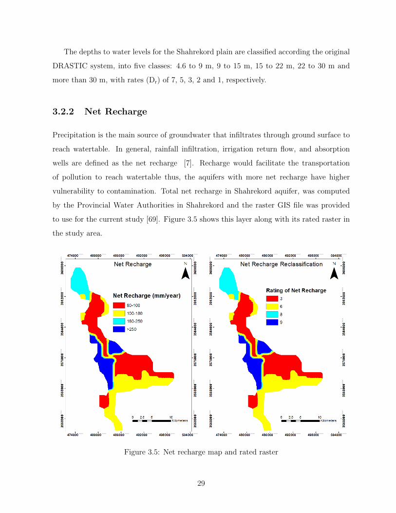
3.2.2 Net Recharge
Precipitation is the main source of groundwater that infiltrates through ground surface to
reach watertable. In general, rainfall infiltration, irrigation return flow, and absorption
wells are defined as the net recharge [7]. Recharge would facilitate the transportation
of pollution to reach watertable thus, the aquifers with more net recharge have higher
vulnerability to contamination. Total net recharge in Shahrekord aquifer, was computed
by the Provincial Water Authorities in Shahrekord and the raster GIS file was provided
to use for the current study [69]. Figure 3.5 shows this layer along with its rated raster in
the study area.
Figure 3.5: Net recharge map and rated raster
29

Net recharge for the Shahrekord plain are classified according the original DRASTIC
system, into four classes: 80 to 100 mm/year, 100 to 180, 180 to 250 mm/year, and more
than 250 mm/year, with net recharge rates (Rr) of 3, 6, 8, and 9, respectively.
3.2.3 Aquifer Media
In this study, classification of aquifer media was determined using a subsurface geology
map, geological sections and drilling logs of the Shahrekord aquifer by the Provincial Water
Authorities. Aquifer media for the Shahrekord plain is classified according to the original
DRASTIC system, into one class which is sand and gravel, with aquifer media rate (Ar) of
8. Aquifer media map was also created using ArcGIS which Figure 3.6 displays its raster
in the study area.
Figure 3.6: Aquifer map and rated raster
30

3.2.4 Soil Media
Soil is considered as the weathered portion above vadose zone which is average 1.8 meter
or less [7]. The soil type is important in terms of amount of net recharge which can
reach the groundwater system. In fact, pollution potential of soil is mainly affected by
the type of clay and grain size of soil. Thus, more clay and smaller grain size implies less
amount of pollution potential [7]. The soil map was used from Soil and Water Institute of
Shahrekord and ratings were assigned according to the original DRASTIC system. Based
on this classification, coarse soil media have high rates in comparison to fine soil media.
Soil media for the Shahrekord plain is classified into three classes which is clay loam, sandy
loam and peat with soil media rate (Sr) of 3, 6 and 8 as displayed in Figure 3.7. It should
be noted that Aller in 1987 emphasized that the maximum rate belonged to gravel, sand,
and sandy loam. Based on the soil media layer, sandy loam was located in majority of
regions in the study area.
Figure 3.7: Soil map and rated raster
31

3.2.5 Topography
Topography indicates the slope of land which controls the probability that a pollutant
will run off or remain on surface to infiltrate [7]. Steeper topographic surfaces are less
vulnerable to contamination. The topography was derived from the Digital Elevation
Model and slope was computed using Spatial Analyst tools in ArcGIS. Then, the obtained
slope map was divided into five classes, which were mostly found in areas with slopes
ranging from 0 to 2 percent which seems reasonable since, the area is mostly agricultural
regions. The classes are 0 to 2 percent, 2 to 6, 6 to 12, 12 to 18 and higher than 18 percent
with slope rate (Tr) of 10, 9, 5, 3 and 1. Figures 3.8 and 3.9 display topography and slope
maps respectively in Shahrekord plain.
Figure 3.8: Topography map
32

Figure 3.9: Slope map and rated raster
3.2.6 Impact of Vadose Zone
Vadose zone is defined as unsaturated zone above watertable [7]. The impact of vadose
zone was classified based on the drilling logs in Shahrekord plain by the Provincial Wa-
ter Authorities. The most significant part of the area included bedded limestone and
sandstone. Therefore, impact of vadose zone was divided into one class, which is bedded
limestone and sandstone with impact of vadose zone rate (Ir) of 6. Figure 3.10 displays
impact of vadose zone layer in Shahrekord plain.
33

Figure 3.10: Impact of vadose zone map and rated raster
3.2.7 Hydraulic Conductivity
In Shahrekord plain, hydraulic conductivity distribution map was generated using pumping
test results and a geoelectrical study of the area by Provincial Water Authorities. Areas
with high levels of hydraulic conductivity can have higher vulnerability to contamination.
Hydraulic conductivity for Shahrekord plain was provided in raster GIS file for using in the
current study which were classified according to the original DRASTIC system, into three
classes: 2.5 to 5 m/day, 4 to 12, 12 to 14 m/day, with hydraulic conductivity rates (Cr) of
1, 2 and 4, respectively. Figure 3.11 displays hydraulic conductivity layer in Shahrekord
plain.
34

Figure 3.11: Hydraulic conductivity map and rated raster
3.3 Nitrate measurements
Since the majority of Shahrekord plain is agricultural with extensive fertilizer application,
therefore nitrate concentration was selected as the main parameter representing the ex-
tent of aquifer pollution. Nitrate has high solubility and mobility which can easily reach
groundwater system even in deep depths. Two monitoring events in 2007 for agricultural
wells, were selected for the construction, analysis and assessment of the original and mod-
ified DRASTIC models in this study. For using nitrate concentration for adjustment and
verification purposes, the result of crop rotation in different years and the effect of ap-
plying various levels of nitrate fertilizer for different crops was considered to be averaged
and uniform across the study area. The first set of samples, a total of fifteen samples,
was obtained in May 2007 and was used for validation purposes and to determine the
35

correlation coefficient between the nitrate concentrations and groundwater vulnerability.
The second set of samples was obtained in July 2007 and was used for modification of
DRASTIC model which were a total of seventeen samples. The geographic positions of
each well was determined using GPS techniques and presented in Figure 3.12.
Figure 3.12: Location of nitrate samples
3.4 Validation methods
Lack of a standard validation method is one of the common reason to criticize DRASTIC
approach. In Shahrekord plain, agriculture is the primary activity and since nitrate does
not exist in groundwater naturally, therefore it can be considered as a good indicator
of pollution. As it was mentioned above, in the current research, nitrate concentration
was measured in 15 monitoring wells in May 2007 in order to verify DRASTIC, modified
36
DRASTIC and reduced models to show whether the vulnerability maps appropriately
represent the actual situation in the study area. This set of data was different from the
set used for model modification purpose. Vulnerability index would increase with the
increasing nitrate concentration in the region. Two methods were used to validate the
obtained models as describe in the below:
3.4.1 Pearson’s correlation coefficient
Pearson’s correlation coefficient (r), as a measure of the linear dependence between two
variables, was calculated between vulnerability indices and observed nitrate concentrations.
3.4.2 Chi-square value
The association of one map with another can be measured and described quantitatively
which is generally useful in a descriptive sense. In the current study, spatial correlation
between DRASTIC map and nitrate map was measured as an area cross-tabulation, with
classes of one map being the rows, and the classes of the second map being the columns.
An area cross-tabulation is a two-dimensional table summarizing the areal overlap of all
possible combination of the two input maps. The chi-square statistic is a measure to
quantity the degree of association between two maps, the calculations are based on the
number from the area cross-tabulation. The area table between map A and map B called
matrix T, with elements Tij, where there are i=1,2,..,n classes of map B (rows of the table)
and j=1,2,..,m classes of map A (columns of the table). The marginal totals of T are
defined as Ti. for the sum of the i-th row, T.j for the sum of the j-th column, and T.. for
the grand total summed over rows and columns [19]. The expected area in each overlap
category is given by the product of marginal totals, divided by grand total. Thus the
expected area Tij* for the i-th row and j-th columns is obtained from Eq. 3.1:
T ∗ij =Ti..T.jT..
(3.1)
37

Then the chi-square statistic is defined as Eq. 3.2:
χ2 =n∑
i=1
m∑j=1
(Tij − T ∗ij)2
T ∗ij(3.2)
similar to the classical chi2 definition (observed-expected)2/expected expression, which
has a lower limit of 0 when the observed areas exactly equal the expected areas and the
two maps are completely independent [19]. As the observed areas become increasingly
different from the expected areas, chi-square increases in magnitude and has a variable
upper limit. The chi-square values can provide an exploratory and descriptive measure
of spatial correlation between maps. In this research, chi-square test was not used as
a statistical test for the significance of the association of the classes of the maps. The
calculated chi-square value was considered only as a relative measure representing the
association of the classes of the two maps. The overall chi-square value represents the
overall association between nitrate map and vulnerability maps and to investigate if the
modified model is improving or degrading the results of DRASTIC in a relative mode,
since their efficiency relatively were compared by their chi-square value.
3.5 Modification methods
There are numerous methods to adjust standard DRASTIC technique that have already
been discussed in literature review chapter. For Shahrekord vulnerability assessment, the
rates and weights of original DRASTIC were modified using Wilcoxon rank sum non-
parametric statistical test and Single Parameter Sensitivity Analysis (SPSA) respectively.
There are some essential requirements in using the Wilcoxon rank sum non-parametric
statistical test, as a rate adjustment technique. One of the most important condition is that
the region must be agricultural. For rate modification, 17 nitrate samples were measured
in July 2007 and the rates of each parameters were rescaled based on average amount of
nitrate located in each class of rated raster. The highest rate (10) will be assigned to the
class with the highest mean of nitrate and other rates were modified linearly based on this
relation. It should be noted that the implementation of the sensitivity analysis requires a
38

well-structured database and a GIS capable of manipulating large tables. Impact of each
parameter in DRASTIC index was also evaluated by using Single Parameter Sensitivity
Analysis (SPSA). The SPSA was used to modify the weight for each layer and comparison
with the original weight in the original DRASTIC.
3.6 Map removal sensitivity analysis
Map removal sensitivity analysis was applied only for the modified DRASTIC model that
showed the highest correlation and similarity with nitrate concentrations. By removing one
or more layers at a time, variation of the vulnerability index were computed. In single map
removal, vulnerability variation index was calculated upon removal of only one layer at a
time. Then, multiple map removal was applied to calculate variation index upon removal
of more than one layer. Based on the obtained results from single map removal, the layers
with less variation were preferentially removed. According to the results of map removal
sensitivity analysis a reduced model with less number of parameters could be suggested.
The reduced model could assess aquifer vulnerability using a fewer parameters in com-
parison with the original DRASTIC model. It should be noted that the DRASTIC index
values of reduced model would be smaller than the values of the full model since it con-
siders fewer parameters. Therefore, in order to compare the reduced and full vulnerability
models, the reduced model should be rescaled. The ratio of lowest (highest) vulnerability
index in reduced model to the lowest (highest) vulnerability index in the full model were
determined. Then the average of calculated ratios were used to rescale of vulnerability in-
dices in the reduced model. It should be noted that, the reduced model was also validated
with a different set of observed nitrate concentrations measured in May 2007.
39

Chapter 4
Results and Discussion
4.1 Original DRASTIC model
All seven required layers for DRASTIC vulnerability evaluation were created using ArcGIS;
each layer was classified and rated using the rating scales based on standard DRASTIC
rating system. Among DRASTIC parameters, the depth to water is one of the most
important parameter with the weight equal to 5. In order to investigate about the effect of
interpolation method used to create this map on the results of vulnerability assessment, two
different interpolation methods; Inverse Distance Weighting (IDW) and Spline were used to
interpolate the depth to water table measured in 25 wells. DRASTIC map was constructed
using both interpolated water depth maps and other six parameters. DRASTIC (IDW)
refers to DRASTIC map obtained from interpolated water depth points using IDW and
other six parameters. Similarly, DRASTIC (spline) refers to the DRASTIC vulnerability
map obtained by interpolated water depth map using spline method along with other
six layers. Then, DRASTIC index which is a dimensionless index, was determined by
multiplying the rated rasters with the weight factor. Figures 4.1 and 4.2 present GIS models
to compute vulnerability index that were created in Model Builder of ArcGIS. Finally, the
obtained index was divided into four classes based on the classification introduced by
Aller in 1987 [7]. The intrinsic (original) vulnerability indices and the corresponding area
percentages for each class are presented in Figures 4.3 and 4.4.
40

Figure 4.1: GIS model to calculate DRASTIC Index (based on IDW interpolation)
Figure 4.2: GIS model to calculate DRASTIC Index (based on spline interpolation)
41

Figure 4.3: Intrinsic vulnerability map and area percentages (IDW)
Figure 4.4: Intrinsic vulnerability map and area percentages (spline)
42

Correlation between original DRASTIC index and nitrate concentrations were used to
validate vulnerability map in the study area. For this purpose, the vulnerability index
in the location of wells were extracted, then Pearson’s correlation was calculated between
DRASTIC indices and nitrate concentrations. As Table 4.1, Figures 4.5 and 4.6 dis-
play, the Pearson’s correlation coefficient for DRASTIC index (IDW) and DRASTIC index
(spline) were -0.24 and -0.3, respectively, showing that the original DRASTIC model could
not properly represent the pollution potential and the vulnerability of this aquifer.
Table 4.1: Correlation factors between nitrate concentrations and intrinsic DRASTIC index
Pearson’s Correlation Coefficient Factor
-0.24 DRASTIC Index (IDW)
-0.3 DRASTIC Index (spline)
Figure 4.5: Correlation between intrinsic DRASTIC index (IDW) and nitrate
43

Figure 4.6: Correlation between intrinsic DRASTIC index (spline) and nitrate
In addition to Pearson’s correlation, DRASTIC (IDW) and DRASTIC (spline) maps
were tested for measuring significant association with nitrate map. For this purpose, nitrate
measurements were interpolated using spline interpolation method to create nitrate map,
then it was classified based on histogram of nitrate values into eight classes as shown in
Figure 4.7.
Moreover, DRASTIC (IDW) and DRASTIC (spline) maps were classified into four
classes based on the standard classification introduced by Aller (1987) [7]. The classes
include; very low (VL) for vulnerability index (less than 100), low (L) for vulnerability
index (100-120), moderate low (ML) for vulnerability index (120-140) and moderate (M)
for vulnerability index (140-160). Then, the correlation between DRASTIC (IDW) and
DRASTIC (spline) maps with nitrate map were evaluated separately using Spatial Analyst
tools (Zonal) in ArcGIS software. The table of area cross-tabulation was the output of
correlation analysis in ArcGIS and the table of chi-square values was calculated from the
number of area cross-tabulation table using Equation 3.2. Tables 4.3 and 4.5 show the
chi-square values calculated from Tables 4.2 and 4.4. The chi-square values for the whole
tables were approximately 39.28 and 25.2 for DRASTIC (IDW) and DRASTIC (spline)
respectively.
44

Figure 4.7: Interpolated nitrate map
Table 4.2: Area cross-tabulation between DRASTIC (IDW) and nitrate (km2)
NitrateClass 1
NitrateClass 2
NitrateClass 3
NitrateClass 4
NitrateClass 5
NitrateClass 6
NitrateClass 7
NitrateClass 8
Total
Class VL 0 6.17 0.36 2.05 1.57 2.89 0 0 13.05Class L 16.26 60.31 25.45 13.44 9.4 25.6 0.35 0.3 151.13Class ML 2.81 22.13 27.6 6.35 11.45 29.43 3.85 0 103.66Class M 0.49 1.01 1.81 2.05 0 0 0 0 5.38Total 19.57 89.63 55.23 23.9 22.43 57.92 4.21 0.3 273
Table 4.3: Chi-square values for DRASTIC (IDW)
NitrateClass 1
NitrateClass 2
NitrateClass 3
NitrateClass 4
NitrateClass 5
NitrateClass 6
NitrateClass 7
NitrateClass 8
Class VL 0.93 0.83 1.96 0.73 0.23 0.005 0.2 0.01Class L 2.72 2.32 0.84 0.003 0.72 1.29 1.68 0.1Class ML 2.85 4.14 2.1 0.81 1.02 2.53 3.2 0.11Class M 0.03 0.31 0.48 5.33 0.44 1.14 0.08 0.006
45

Table 4.4: Area cross-tabulation between DRASTIC (spline) and nitrate (km2)
NitrateClass 1
NitrateClass 2
NitrateClass 3
NitrateClass 4
NitrateClass 5
NitrateClass 6
NitrateClass 7
NitrateClass 8
Total
Class VL 0.01 7.26 0.77 2.42 2.04 4.12 0.2 0.26 17.1Class L 12.1 47.91 25.5 14.97 11.33 27.46 0.21 0.03 139.56Class ML 6.47 33.06 25.43 4.51 8.67 26.14 3.78 0 108.1Class M 0.99 1.39 3.5 1.99 0.37 0 0 0 8.26Total 19.57 89.63 55.23 23.9 22.43 57.74 4.21 0.3 273
Table 4.5: Chi-square values for DRASTIC (spline)
NitrateClass 1
NitrateClass 2
NitrateClass 3
NitrateClass 4
NitrateClass 5
NitrateClass 6
NitrateClass 7
NitrateClass 8
Class VL 1.2 0.48 2.08 0.56 0.29 0.07 0.01 3.22Class L 0.43 0.09 0.26 0.62 0.001 0.14 1.73 0.09Class ML 0.21 0.16 0.58 2.59 0.004 0.47 2.69 0.11Class M 0.26 0.64 2.01 2.23 0.13 1.74 0.12 0.009
The larger value of chi-square means that two maps are more spatially dependent.
Above results indicated the values of chi-square for DRASTIC (IDW) is larger in compar-
ison with the chi-square calculated for DRASTIC (spline). These values are not helpful in
this step because there is no basis for judging how significant these values were but there
was a good consistency with the results obtained from Pearson’s correlation coefficient.
The comparison between the original DRASTIC values and validation nitrate samples
of 15 wells in May 2007 are displayed in Figures 4.8 and 4.9. As the results of cor-
relation showed, the vulnerability mapping for Shahrekord aquifer does not conform to
concentrations of nitrate measured in the monitoring wells. This means that the intrinsic
vulnerability index calculated by the original DRASTIC model cannot properly represent
the pollution potential for this aquifer and must be modified according to specification of
study area and nitrate contaminant in order to present a more realistic evaluation of the
pollution potential. As the first step, rate modification techniques were applied to calibrate
DRASTIC algorithm and then the weights of each parameter were modified using Single
Parameter Sensitivity Analysis (SPSA) approach as discussed in the following section.
46

Figure 4.8: Nitrate validation samples on DRASTIC (IDW) map
Figure 4.9: Nitrate validation samples on DRASTIC (spline) map
47

4.2 Rate modification using nitrate concentrations
Due to extensive fertilizer application through intense agricultural activities in the region,
nitrate concentration is considered as the main source of pollution. The observed nitrate
measured at 17 monitoring wells in July 2007 was used to modify the rates of parameters
in DRASTIC model. The ranking system derived of Wilcoxon rank sum non-parametric
statistical test was used as a rate adjustment technique for vulnerability mapping in the
Shahrekord aquifer. The rates of parameters were rescaled based on the average amount of
nitrate concentration in each class for each layer, then the highest rate (10) was assigned
to the class with the highest mean of nitrate concentration and other rates were modified
linearly based on this relation. Aquifer media and impact of vadose zone have only one
class in all the region therefore, in the current study, only the rates of the depth to water,
net recharge, soil media, topography and hydraulic conductivity were modified based on
the mean nitrate concentration. Using 17 samples collected in July 2007, the rates of orig-
inal DRASTIC were modified. Parameter classes, as well as the corresponding rating of
each class, the average nitrate concentrations and the respective modified rating of every
class or group of classes are presented in Table 4.6.
48

Table 4.6: Standard and modified DRASTIC rates based on nitrate concentrations
Parameter Range Standard rate Mean NO3 (mg/l) Modified rateDepth to water (Spline) (m) 4.5-9 7 17.75 5.56
9-15 5 10.65 3.3315-22 3 21.02 6.5822-30 2 15.38 4.81>30 1 31.95 10
Depth to water (IDW) (m) 4.5-9 7 17.75 5.889-15 5 19.53 6.4715-22 3 17.16 5.6922-30 2 30.18 10>30 1 No data 1
Net Recharge (mm) 80-100 3 21.3 10100-180 6 17.75 8.33180-250 8 17.75 8.33>250 9 14.2 6.67
Soil Media Clay loam 3 22.48 10Sandy loam 6 18.26 8.12Peat 8 No data 8
Topography (Slope%) 0-2 10 19.64 102-6 9 14.23 7.246-12 5 No data 512-18 3 No data 3>18 1 No data 1
Conductivity (m/day) 2.5-4 1 14.2 44-12 2 20.24 5.712-14 4 35.5 10
In order to compare the rates used to calculate the original and modified-rates DRAS-
TIC index, the statistical summary of rates are provided in Tables 4.7 and 4.8. In original
DRASTIC, the highest risk of contamination (mean rates of 8 and 9) of groundwater in
Shahrekord aquifer originated from aquifer media and the topography parameters. The
soil media, net recharge and impact of vadose zone had moderate risks of contamination
(5 and 6) while depth to water and hydraulic conductivity imposed a low risk of aquifer
contamination (3 and 1). Depth to water, net recharge and hydraulic conductivity showed
moderate variation (CV% are 43, 41 and 39, respectively) while soil media and topogra-
phy were less variable (CV% are 24 and 14, respectively). In modified-rates DRASTIC,
49

the highest risk of contamination (8 and 9) of groundwater originated from net recharge,
aquifer media, soil media and the topography parameters while depth to water, hydraulic
conductivity and impact of vadose zone had moderate effect on risk of contamination (5
and 6). Depth to water and hydraulic conductivity were moderately variable (CV% are
30 and 26, respectively) while soil media, net recharge and topography were less variable
(CV% are 9, 13 and 17, respectively). Also in both original and modified-rates DRASTIC
models, the rate of aquifer media and impact of vadose zone were constant in the whole
area.
Table 4.7: Statistical summary of rates in original DRASTIC
D (IDW) D (spline) R A S T I CMinimum 1 1 3 8 3 1 6 1Maximum 7 7 9 8 8 10 6 4Mean 3.19 3.33 5.43 8 5.32 9.51 6 1.87SD 1.11 1.44 2.25 - 1.32 1.36 - 0.73CV(%) 34 43 41 - 24 14 - 39
S.D. stands for standard deviation and CV for coefficient of variation.
Table 4.8: Statistical summary of rates in modified-rates DRASTIC
D (IDW) D (spline) R A S T I CMinimum 1 3.33 6.67 8 8 1 6 4Maximum 10 10 10 8 10 10 6 10Mean 6.4 5.6 8.7 8 8.56 9.19 6 5.55SD 1.87 1.7 1.15 - 0.79 1.62 - 1.44CV(%) 29 30 13 - 9 17 - 26
S.D. stands for standard deviation and CV for coefficient of variation.
All DRASTIC layers except aquifer media and impact of vadose zone were reclassified
by ArcGIS, based on new rates which were calculated using nitrate concentrations. The
modified-rates DRASTIC (IDW) and modified-rates DRASTIC (spline) indices were cal-
culated and divided into four groups based on Aller’s classification. Figures 4.10 and 4.11
display the modified-rates vulnerability maps and their corresponding area percentages.
After rate modification and assigning the highest rate (10) to the class with the highest
average mount of nitrate, the vulnerability indices increased considerably. It can be jus-
tified that vulnerability mapping classes are not absolute and in a relative mode it maps
50

the relative vulnerability of the study area.
Figure 4.10: Modified-rates DRASTIC (IDW) map and area percentages
51

Figure 4.11: Modified-rates DRASTIC (spline) map and area percentages
52

The modified-rates DRASTIC (IDW) map indicated that 43.4 and 13% of the area
belonged to the moderate-high and high vulnerability classes respectively. The percentages
for these classes were zero before the rate modification. The percentages for the moderate-
low and moderate classes after rate modification were 1 and 42.6 %, respectively, which
were 32 and 2% in the original DRASTIC (IDW) model. The same trend was observed
when comparing modified-rates DRASTIC (spline) model with original DRASTIC (spline)
model.
In order to validate the modified-rates DRASTIC maps, Pearson’s correlation between
modified-rates DRASTIC index and nitrate concentrations in the 15 monitoring wells were
computed. Samples with nitrate values used for this validation are different from the ones
applied in DRASTIC modification. The Pearson’s correlation for modified-rates DRASTIC
index (IDW) and modified-rates DRASTIC index (spline) were computed which increased
to 0.64 and 0.84, respectively, as indicated in Table 4.9 and Figures 4.12 and 4.13. The
results showed that the modified-rates DRASTIC model now can adequately represent the
extent of pollution measured as nitrate concentrations in groundwater. In other words,
using modified-rates DRASTIC model, it was possible to obtain a more accurate assess-
ment for groundwater vulnerability in the Shahrekord. Moreover, the results revealed that
vulnerability map might vary based on the interpolation method (IDW or spline) used to
interpolate depth to water points, since modified-rates DRASTIC (spline) had a higher
correlation with nitrate concentrations in compared to modified-rates DRASTIC (IDW)
model.
Table 4.9: Correlation factors between nitrate and modified-rates DRASTIC index
Pearson’s Correlation Coefficient Factor
0.64 Modified-rates DRASTIC Index (IDW)
0.84 Modified-rates DRASTIC Index (spline)
53
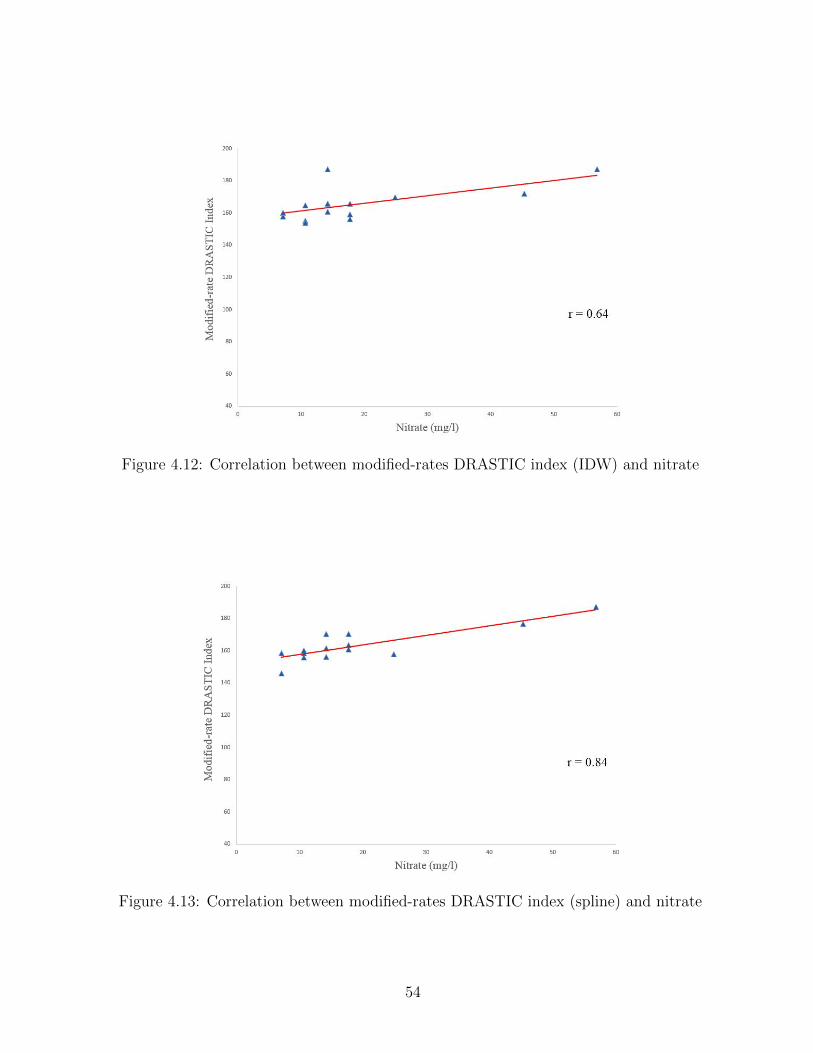
Figure 4.12: Correlation between modified-rates DRASTIC index (IDW) and nitrate
Figure 4.13: Correlation between modified-rates DRASTIC index (spline) and nitrate
54

To further investigate the accuracy of modified-rates DRASTIC maps, correlation be-
tween nitrate map and modified-rates DRASTIC maps were measured. For this purpose,
the modified-rates DRASTIC (IDW) and modified-rates DRASTIC (spline) maps were
classified based on the standard classification introduced by Aller (1987) into four classes
including moderate low (ML) for vulnerability index (120-140), moderate (M) for vulnera-
bility index (140-160), moderate high (MH) for vulnerability index (160-180) and high (H)
for vulnerability index (180-200). The classification and creation of nitrate map were dis-
cussed in the section of original DRASTIC validation. Tables 4.11 and 4.13 are shown the
chi-square values calculated from area cross-tabulation results shown in Tables 4.10 and
4.12. The total chi-square value which is the summation of all values in chi-square table,
are approximately 59.04 and 58.34 for modified-rates DRASTIC (IDW) and modified-rates
DRASTIC (spline) respectively.
Table 4.10: Area cross-tabulation between modified-rates DRASTIC (IDW) and nitrate(km2)
NitrateClass 1
NitrateClass 2
NitrateClass 3
NitrateClass 4
NitrateClass 5
NitrateClass 6
NitrateClass 7
NitrateClass 8
Total
Class ML 0 0 0 0 0 2.75 0 0 2.75Class M 13.23 31.43 29.35 9.48 10.15 22.25 0.45 0 116.37Class MH 6.57 51.23 25.56 10.74 4.04 17.03 3.38 0 118.58Class H 0.04 6.92 0.82 3.54 8.25 15.6 0.31 0.27 35.79Total 19.85 89.58 55.74 23.77 22.44 57.65 4.16 0.27 273
Table 4.11: Chi-square values for modified-rates DRASTIC (IDW)
NitrateClass 1
NitrateClass 2
NitrateClass 3
NitrateClass 4
NitrateClass 5
NitrateClass 6
NitrateClass 7
NitrateClass 8
Class ML 0.2 0.9 0.56 0.23 0.22 8.15 0.04 0.002Class M 2.71 1.17 1.33 0.03 0.03 0.21 0.97 0.11Class MH 0.48 3.95 0.08 0.01 3.32 2.53 1.38 0.12Class H 2.5 1.96 5.74 0.06 9.61 8.61 0.09 1.6
55

Table 4.12: Area cross-tabulation between modified-rates DRASTIC (spline) and nitrate(km2)
NitrateClass 1
NitrateClass 2
NitrateClass 3
NitrateClass 4
NitrateClass 5
NitrateClass 6
NitrateClass 7
NitrateClass 8
Total
Class ML 0.98 3.75 3.63 1.92 0.6 0 0 0 10.89Class M 12.59 49.51 27.47 7.87 9.52 17.09 0.65 0 124.73Class MH 6.27 36.3 24.28 13.89 11.37 27.58 29.8 0.07 122.77Class H 0 0.02 0.33 0.08 0.94 12.89 0.52 0.2 15.01Total 19.85 89.58 55.73 23.77 22.44 57.58 4.16 0.27 273
Table 4.13: Chi-square values for modified-rates DRASTIC (spline)
NitrateClass 1
NitrateClass 2
NitrateClass 3
NitrateClass 4
NitrateClass 5
NitrateClass 6
NitrateClass 7
NitrateClass 8
Class ML 0.04 0.009 0.89 1 0.09 2.29 0.16 0.01Class M 1.38 1.82 0.16 0.81 0.05 3.2 0.81 0.12Class MH 0.77 0.38 0.02 0.96 0.16 0.11 0.67 0.02Class H 1.09 4.87 2.42 1.14 0.06 29.97 0.37 2.37
As the results of Pearson’s correlation coefficient and chi-square value indicated, there
was a much higher correlation between modified-rates DRASTIC (IDW) and modified-rates
DRASTIC (spline) with nitrate concentrations in comparison with their corresponding
correlations in the original DRASTIC models. The correlation coefficient and chi-square
value for modified-rates DRASTIC (IDW) were obtained as 0.64 and 59.04 whereas these
values were calculated as -0.24 and 39.28 for the original DRASTIC (IDW). Also, for
modified-rates DRASTIC (spline), the Pearson’s correlation coefficient and chi-square value
were calculated as 0.84 and 58.34 whereas these values were -0.3 and 25.2 for the original
DRASTIC (spline). The values of chi-square increased after rate modification and it can
be concluded that there was more spatial association between modified-rates DRASTIC
maps and nitrate map in comparison to the original DRASTIC model. Also, there was
a good consistency between the results of Pearson’s correlation and chi-square value. As
the results demonstrated, the modified-rates DRASTIC model was better able to predict
pollutant areas than the original model. Figures 4.14 and 4.15 compare the modified-rates
DRASTIC vulnerability maps and the nitrate concentrations visually.
56

Figure 4.14: Nitrate validation samples on modified-rates DRASTIC (IDW) map
Figure 4.15: Nitrate validation samples on modified-rates DRASTIC (spline) map
57
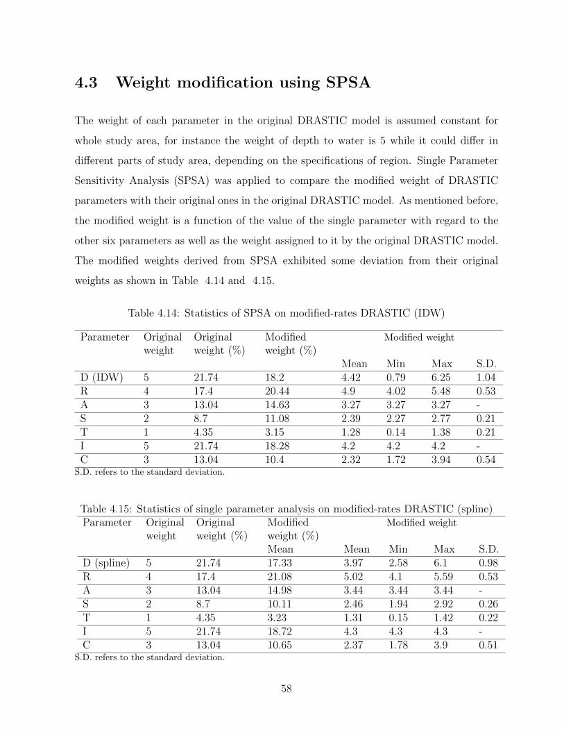
4.3 Weight modification using SPSA
The weight of each parameter in the original DRASTIC model is assumed constant for
whole study area, for instance the weight of depth to water is 5 while it could differ in
different parts of study area, depending on the specifications of region. Single Parameter
Sensitivity Analysis (SPSA) was applied to compare the modified weight of DRASTIC
parameters with their original ones in the original DRASTIC model. As mentioned before,
the modified weight is a function of the value of the single parameter with regard to the
other six parameters as well as the weight assigned to it by the original DRASTIC model.
The modified weights derived from SPSA exhibited some deviation from their original
weights as shown in Table 4.14 and 4.15.
Table 4.14: Statistics of SPSA on modified-rates DRASTIC (IDW)
Parameter Originalweight
Originalweight (%)
Modifiedweight (%)
Modified weight
Mean Min Max S.D.D (IDW) 5 21.74 18.2 4.42 0.79 6.25 1.04R 4 17.4 20.44 4.9 4.02 5.48 0.53A 3 13.04 14.63 3.27 3.27 3.27 -S 2 8.7 11.08 2.39 2.27 2.77 0.21T 1 4.35 3.15 1.28 0.14 1.38 0.21I 5 21.74 18.28 4.2 4.2 4.2 -C 3 13.04 10.4 2.32 1.72 3.94 0.54
S.D. refers to the standard deviation.
Table 4.15: Statistics of single parameter analysis on modified-rates DRASTIC (spline)Parameter Original
weightOriginalweight (%)
Modifiedweight (%)
Modified weight
Mean Mean Min Max S.D.D (spline) 5 21.74 17.33 3.97 2.58 6.1 0.98R 4 17.4 21.08 5.02 4.1 5.59 0.53A 3 13.04 14.98 3.44 3.44 3.44 -S 2 8.7 10.11 2.46 1.94 2.92 0.26T 1 4.35 3.23 1.31 0.15 1.42 0.22I 5 21.74 18.72 4.3 4.3 4.3 -C 3 13.04 10.65 2.37 1.78 3.9 0.51
S.D. refers to the standard deviation.
58

According to results of weight modification, net recharge had the highest effect in the
vulnerability evaluation because it also had the highest mean modified weight among all
other parameters. Also, the soil media and aquifer media showed high modified weight
(11.08 and 14.63% for DRASTIC (IDW), 10.11 and 14.98% for DRASTIC (spline) that
exceeds the original weights assigned by DRASTIC (8.7 and 13.04 %). The rest of the
parameters exhibited lower weights compared to the original weights. Using column chart,
the value of weights before and after modification can be compared visually as shown in
Figures 4.16 and 4.17.
Figure 4.16: Comparison of weights of parameters before and after modification (IDW)
Figure 4.17: Comparison of weights of parameters before and after modification (spline)
59
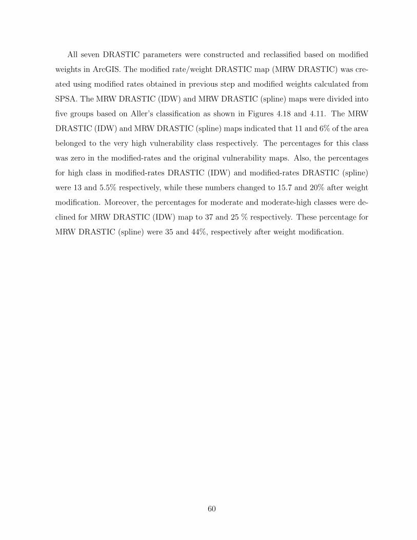
All seven DRASTIC parameters were constructed and reclassified based on modified
weights in ArcGIS. The modified rate/weight DRASTIC map (MRW DRASTIC) was cre-
ated using modified rates obtained in previous step and modified weights calculated from
SPSA. The MRW DRASTIC (IDW) and MRW DRASTIC (spline) maps were divided into
five groups based on Aller’s classification as shown in Figures 4.18 and 4.11. The MRW
DRASTIC (IDW) and MRW DRASTIC (spline) maps indicated that 11 and 6% of the area
belonged to the very high vulnerability class respectively. The percentages for this class
was zero in the modified-rates and the original vulnerability maps. Also, the percentages
for high class in modified-rates DRASTIC (IDW) and modified-rates DRASTIC (spline)
were 13 and 5.5% respectively, while these numbers changed to 15.7 and 20% after weight
modification. Moreover, the percentages for moderate and moderate-high classes were de-
clined for MRW DRASTIC (IDW) map to 37 and 25 % respectively. These percentage for
MRW DRASTIC (spline) were 35 and 44%, respectively after weight modification.
60

Figure 4.18: MRW DRASTIC map and area percentages (IDW)
Figure 4.19: MRW DRASTIC map and area percentages (spline)
61

In order to validate the MRW DRASTIC (IDW) and the MRW DRASTIC (spline)
maps, correlation between MRW DRASTIC vulnerability index and 15 nitrate concen-
trations were computed. Table 4.16 and Figures 4.20 and 4.21 display the results of
correlation calculation. The correlation coefficient for both MRW DRASTIC (IDW) and
MRW DRASTIC (spline) increased to 0.7 and 0.88, respectively, after weight modification.
Table 4.16: Correlation factors between nitrate and MRW DRASTIC index
Pearson’s Correlation Coefficient Factor
0.7 MRW DRASTIC Index (IDW)
0.88 MRW DRASTIC Index (spline)
Figure 4.20: Correlation between MRW DRASTIC index and nitrate (IDW)
62

Figure 4.21: Correlation between MRW DRASTIC index and nitrate (spline)
To investigate if there was any improvements in the vulnerability models after weight
modification, the models were tested by calculating chi-square for nitrate map with MRW
DRASTIC (IDW) and MRW DRASTIC (spline) maps. The MRW DRASTIC (IDW) and
MRW DRASTIC (spline) were classified into five classes including; moderate low (ML) for
vulnerability index (120-140), moderate (M) for vulnerability index (140-160), moderate
high (MH) for vulnerability index (160-180), high (H) for vulnerability index (180-200)
and very high (VH) for vulnerability index (above 200). The preparation of nitrate map
was the same with previous validation section. Area cross-tabulation table was obtained
by using available tools in ArcGIS, then chi-square value table was calculated based on the
numbers in cross-tabulation table. Tables 4.18 and 4.20 are shown the chi-square values
calculated from Tables 4.17 and 4.19. The chi-square values for the whole tables are
approximately 39.38 and 72.93 for MRW DRASTIC (IDW) and MRW DRASTIC (spline)
models respectively. The correlation coefficient and chi-square value for MRW DRASTIC
(IDW) were obtained as 0.7 and 39.38 whereas these values were calculated as -0.24 and
39.28 for the original DRASTIC (IDW). Also, for MRW DRASTIC (spline), the Pearson’s
correlation coefficient and chi-square value were calculated as 0.88 and 72.93 whereas these
values were -0.3 and 25.2 for the original DRASTIC (spline).
63

Table 4.17: Area cross-tabulation between MRW DRASTIC (IDW) and nitrate (km2)
NitrateClass 1
NitrateClass 2
NitrateClass 3
NitrateClass 4
NitrateClass 5
NitrateClass 6
NitrateClass 7
NitrateClass 8
Total
Class ML 0 0 0.35 0.04 0.13 0.26 0 0 0.79Class M 5.05 25.3 27.7 9.36 9.43 24.3 0.6 0 101.77Class MH 9.65 37.61 21.58 9.82 4.62 14.31 0.62 0 98.25Class H 0.7 19.94 5.49 1.29 4.27 9.09 2.61 0 43.41Class VH 4.46 6.98 0.83 3.49 3.98 10.16 0.31 0.27 30.51Total 19.88 89.84 55.96 24.03 22.44 58.15 4.16 0.27 274
Table 4.18: Chi-square values for MRW DRASTIC (IDW)
NitrateClass 1
NitrateClass 2
NitrateClass 3
NitrateClass 4
NitrateClass 5
NitrateClass 6
NitrateClass 7
NitrateClass 8
Class ML 0.05 0.26 0.21 0.006 0.07 0.05 0.01 0.0008Class M 0.72 1.91 2.34 0.02 0.15 0.35 0.56 0.1Class MH 0.91 0.93 0.12 0.17 1.44 2.01 0.49 0.09Class H 1.89 2.32 1.26 1.64 0.14 0.0009 5.81 0.04Class VH 2.3 0.9 4.65 0.25 0.88 2.12 0.04 1.98
Table 4.19: Area cross-tabulation between MRW DRASTIC (spline) and nitrate (km2)
NitrateClass 1
NitrateClass 2
NitrateClass 3
NitrateClass 4
NitrateClass 5
NitrateClass 6
NitrateClass 7
NitrateClass 8
Total
Class ML 0.89 3.92 5.66 2.57 0.6 0.06 0 0 13.72Class M 7.28 21.11 16.86 3.9 9.15 10.6 0.18 0 69.11Class MH 10 50.75 16.62 8.51 8.8 23.67 1.56 0.07 120.03Class H 0.68 14.02 16.46 8.94 2.92 10.3 1.89 0 55.26Class VH 1 0.02 0.32 0.08 0.94 13.43 0.52 0.2 16.54Total 19.88 89.84 55.96 24.03 22.44 58.08 4.16 0.27 274
Table 4.20: Chi-square values for MRW DRASTIC (spline)
NitrateClass 1
NitrateClass 2
NitrateClass 3
NitrateClass 4
NitrateClass 5
NitrateClass 6
NitrateClass 7
NitrateClass 8
Class ML 0.009 0.07 2.94 1.57 0.23 2.78 0.2 0.01Class M 1.04 0.09 0.55 0.75 2.18 1.1 0.71 0.07Class MH 0.2 3.36 2.5 0.37 0.1 0.11 0.03 0.01Class H 2.73 0.9 2.41 3.48 0.55 0.16 1.34 0.05Class VH 0.03 5.36 2.74 1.28 0.12 28.21 0.29 2.13
64

The larger value of chi-square implies that two maps were more spatially dependent.
As the results indicated, the values of chi-square increased after rate and weight modifi-
cations. It means that MRW DRASTIC maps can better represent the observed nitrate
concentrations in the study area. Both validation results, Pearson’s correlation coefficient
and chi-square value, demonstrated that MRW DRASTIC (spline) was the best vulnera-
bility map to present contamination situation in the Shahrekord plain. The highest value
of Pearson’s correlation coefficient (0.88) and chi-square value (72.93) belonged to MRW
DRASTIC (spline) map.
The visual comparison between the MRW DRASTIC index values and the nitrate con-
centrations are displayed in Figures 4.22 and 4.23. The results showed that Pearson’s
correlation coefficient for the MRW DRASTIC (IDW) increased to 0.7 compared to 0.64
before weight modification. Also, this improvement was remarkable for the MRW DRAS-
TIC (spline), since it increased from 0.84 to 0.88 after weight modification. This values
indicated that there are relatively high correlation between obtained modified vulnerability
models and nitrate validation samples.
Figure 4.22: Nitrate validation samples on MRW DRASTIC (IDW) map
65

Figure 4.23: Nitrate validation samples on MRW DRASTIC (spline) map
4.4 Map removal sensitivity analysis
The map removal sensitivity analysis determines the sensitivity of vulnerability map to
remove one or more layers from vulnerability map. This sensitivity can be computed in
terms of variation index using the Equation 2.2, as explained in chapter 2. In the current
study, the map removal sensitivity analysis were applied for MRW DRASTIC (spline) map
which had the best Pearson’s correlation coefficient (0.88) and chi-square value (72.93). The
results were calculated by removing one or more layers at a time in a stepwise approach.
Table 4.21 shows the variation of the vulnerability index as a result of removing only
one layer at a time. It is obvious that high variation of the vulnerability index is expected
upon the removal of the net recharge parameter from the calculation. This could mainly be
attributed to the relatively high modified weight assigned to this layer which was presented
in Table 4.15 and the high recharge rate characteristic of the Shahrekord aquifer (mean
rating score after rate modification is 8.7).
66

Table 4.21: Statistics of single map removal sensitivity analysis
Parameter removed Variation index(%)
Max Mean Min S.D.Depth to water (D) 2.83 0.86 0 0.56Net Recharge (R) 4.03 2 0.32 0.86Aquifer Media (A) 1.35 0.39 0.02 0.25Soil Media (S) 4.46 0.59 0 0.38Topography (T) 2.36 1.15 0.54 0.35Impact of Vadose (I) 1.11 0.26 0 0.2Hydraulic Conductivity (C) 1.8 1.16 0.3 0.32
In order to apply multiple map removal (removal of more than one layer), the layers were
removed based on the results from previous map removal sensitivity measures (Table 4.22).
The layers, which had less variation of the final vulnerability index, were preferentially
removed. The least average variation index resulted after removing only the impact of
vadose zone layer (0.26%). As more layers were excluded from the calculation of the
vulnerability index, the mean variation index increased. In general, considerable variation
in the vulnerability assessment is expected if a lower number of data layers have been used.
Table 4.22: Statistics of multiple map removal sensitivity analysis
Parameter used Variation Index(%)
Max Mean Min S.D.D,R,A,S,T and C 1.11 0.26 0 0.2D,R,S,T and C 2.96 0.75 0 0.57D,R,T and C 4.78 1.13 0 0.96R,T and C 5.24 1.54 0 1.05R and C 9.24 3.31 0 2.18R 24.22 12 1.92 5.19
After single and multiple map removal, the vulnerability maps were created for all
possible cases in ArcGIS. In order to validate the constructed maps, Pearson’s correlation
coefficients were computed between new vulnerability maps and nitrate concentrations.
The results of correlation calculations are displayed in Tables 4.23 and 4.24. The results
indicated that removal of aquifer media (A), topography (T) and impact of vadose zone
67

(I) had the least effect on the correlation coefficient as it expected. It might be concluded
that these parameters have less effect than the other layers.
Table 4.23: Correlation between nitrate and vulnerability map obtained from single mapremoval
Parameter removed Pearson’s Correlation CoefficientDepth to water (D) 0.52Net Recharge (R) 0.46Aquifer Media (A) 0.88Soil Media (S) 0.47Topography (T) 0.89Impact of Vadose (I) 0.88Hydraulic Conductivity (C) 0.68
Table 4.24: Correlation between nitrate and vulnerability map obtained from multiple mapremoval
Parameter(s) removed Parameter(s) used Pearson’s Correlation CoefficientI D,R,A,S,T and C 0.88I and A D,R,S,T and C 0.88I,A and S D,R,T and C 0.82I,A,S and D R,T and C 0.52I,A,S,D and T R and C 0.53I,A,S,D,T and C R 0.12
Aquifer media (A), Topography (T) and Impact of vadose zone (I) indicated no effect
on MRW DRASTIC (spline) index, therefore in order to further investigate the sensitivity
of vulnerability map to removing these parameters, MRW DRASTIC (spline) map was
constructed only by using Depth to water, Net recharge, Soil media, Hydraulic conductiv-
ity layers. Figure 4.24 displays the reduced MRW DRASTIC (spline) map for Shahrekord
aquifer which was created by eliminating A, T and I. Comparison of reduced MRW DRAS-
TIC (spline) and full MRW DRASTIC (spline) models in Figure 4.25, it was found that
the region of higher vulnerability in both maps was situated in southeastern part of the
study area. Nitrate concentration measurements were shown on the same maps for visual
comparison.
68

Figure 4.24: Reduced MRW DRASTIC (spline) map
Figure 4.25: Comparison between full and reduced MRW DRASTIC (spline) maps
69

In order to ensure that the reduced MRW DRASTIC map is reliable enough, it was
validated by observed nitrate concentrations. The Pearson’s correlation between reduced
MRW DRASTIC index and nitrate concentrations demonstrated a high coefficient of 0.88
as displayed in Figure 4.26.
Figure 4.26: Correlation between reduced MRW DRASTIC (spline) index and nitrate
Also, the correlation between nitrate map and reduced MRW DRASTIC map was
measured by calculating chi-square value. The relationship between these two maps was
apparent as indicated in Tables 4.25 and 4.26. The total chi-square which is the total of
values in chi-square table was calculated as 100.38 for reduced MRW DRASTIC model.
Table 4.25: Area cross-tabulation between reduced MRW DRASTIC map and nitrate(km2)
NitrateClass 1
NitrateClass 2
NitrateClass 3
NitrateClass 4
NitrateClass 5
NitrateClass 6
NitrateClass 7
NitrateClass 8
Total
Class L 0 1.08 5.58 2.49 0.61 0 0 0 9.76Class ML 0.94 5.78 8.04 1.41 1.19 2.51 0 0 19.87Class M 11.2 16.1 8.61 2.57 8.09 6.7 0.16 0 53.43Class MH 0.09 38.1 15.11 6.1 7.78 24.89 1.57 0.1 94.55Class H 5.3 28.09 17.86 9.47 3.85 8.12 0.19 0 72.88Class VH 1.54 1.52 0.59 1.92 1.02 16.16 2.21 0.24 25.2Total 19.88 90.67 55.79 23.96 22.54 53.38 4.13 0.34 275
70

Table 4.26: Chi-square values for reduced MRW DRASTIC (spline) map
NitrateClass 1
NitrateClass 2
NitrateClass 3
NitrateClass 4
NitrateClass 5
NitrateClass 6
NitrateClass 7
NitrateClass 8
Class L 0.7 1.41 6.57 3.17 0.04 2.06 0.14 0.01
Class ML 0.17 0.09 4.01 0.05 0.11 0.68 0.29 0.02
Class M 14.01 0.12 0.44 0.92 3.17 1.88 0.51 0.06
Class MH 5.14 1.58 0.84 0.54 0.0003 1.88 0.01 0.002
Class H 0 0.71 0.65 1.55 0.74 3.46 0.74 0.08
Class VH 0.04 5.53 3.98 0.03 0.52 21.95 8.89 1.4
According to the validation results, the reduced MRW DRASTIC (spline) model had
Pearson’s correlation coefficient of 0.88 which was the same with the full MRW DRASTIC
spline) model (0.88) and the chi-square value was obtained as 100.38 which was higher than
the chi-square value in full model (72.93). The larger value of chi-square indicated a remark-
able similarity between the reduced model and nitrate map. Therefore, it can be concluded
that the vulnerability map for Shahrekord plain obtained from reduced MRW DRASTIC
(spline) model could be considered as reliable as the full MRW DRASTIC (spline) model
including all seven layers. Thus, it can be possible to assess Shahrekord vulnerability
with fewer parameters in compared to seven parameters in the original DRASTIC model.
The advantage of this investigation was the efficiency and capability of vulnerability map
obtained from only 4 parameters than seven layers.
71

4.5 Discussion
In the current study, two nitrate data sets were measured during two monitoring events
in May and July 2007 were measured for modification and verification purposes. Nitrate
concentrations obtained in July 2007 was used to modify the rates of parameters. All
modified models were validated by samples from May 2007. Pearson’s correlation factor and
chi-square value were calculated to quantify the spatial dependency between nitrate map
and vulnerability maps. According to results of validation, among all modified DRASTIC
models, the MRW DRASTIC (spline) was more reliable map to represent vulnerability
conditions in Shahrekord plain.
Map removal sensitivity analysis and SPSA demonstrated that the removal of net
recharge caused larger variation in vulnerability index, since this parameter had a rela-
tively high modified weight among other parameters. After single map removal, vulnera-
bility maps were created for all cases, then Pearson’s correlation was calculated between
new vulnerability index and observed nitrate concentrations. The results indicated that
Aquifer media, Topography and Impact of vadose zone had the least effective in Shahrekord
vulnerability assessment. Therefore, a reduced model was proposed using only Depth to
water, Net recharge, Soil media and Hydraulic conductivity for Shahrekord vulnerability
evaluation. The reduced model was also validated using observed nitrate concentrations
and the results demonstrated a high Pearson’s correlation coefficient and chi-square value.
Therefore, it can be concluded that the reduced model is reliable as the full model for
Shahrekord vulnerability assessment.
Statistical spatial association between DRASTIC maps (original and modified) and
nitrate map were tested using map pair analysis. Chi-square value was calculated as a
relative measure to define the spatial dependency between two maps. A larger chi-square
value implies higher association and spatial dependency. In this research, this value was
considered for comparing the efficiency of modified models to the original ones to see if the
new approach is improving or degrading the results of DRASTIC vulnerability assessment.
72

Chapter 5
Conclusion
5.1 Summary
The Shahrekord plain is located in a semi-arid region which groundwater is the main water
source in the area. Due to extensive cultivation with intense fertilizer application, nitrate
concentrations in the groundwater are considered the primary source of pollution. DRAS-
TIC model was applied for aquifer vulnerability evaluation in the study area. All seven
required hydrogeological layers comprising Depth to water, net Recharge, Aquifer media,
Soil media, Topography, Impact of vadose zone and hydraulic Conductivity (DRASTIC)
were created and rated in ArcGIS. The depth to water points which was measured in 25 ob-
servation wells, was interpolated using two methods including Inverse Distance Weighting
(IDW) and spline. In order to validate the obtained DRASTIC map, the measured nitrate
concentrations in agricultural wells were used to correlate the pollution in the aquifer to the
DRASTIC index. The Pearson’s correlation factor indicated that the original DRASTIC
model could not provide a satisfactory intrinsic vulnerability evaluation of groundwater to
pollution. Therefore, the original DRASTIC algorithm required modification to obtain a
more reliable results. The rates and weights of original DRASTIC model were modified
using Wilcoxon rank sum non-parametric statistical test and Single Parameter Sensitivity
Analysis (SPSA) respectively. The modified-rates DRASTIC and MRW DRASTIC models
were developed and to measure any improvements in new models, the Pearson’s correlation
73

coefficient and chi-square value were calculated. The MRW DRASTIC (spline) map showed
the best correlation coefficient (0.88) and chi-square value (72.93) among all modified vul-
nerability maps. For MRW DRASTIC (spline) map, the variation of vulnerability index
was tested by single and multiple map removal sensitivity analysis. The results revealed
that the removal of net recharge caused larger variation in MRW DRASTIC (spline) index
indicating that this parameter had more impact on the DRASTIC vulnerability of the
aquifer. Moreover, Aquifer media, Topography and Impact of vadose zone were found not
to have a significant effect in assessing Shahrekord aquifer vulnerability. Consequently, a
reduced model was introduced with less number of parameters and as a results less amount
of required input data for Shahrekord vulnerability mapping containing four parameters;
Depth to water, Net Recharge, Soil media, Hydraulic Conductivity. The reduced model
was also validated using nitrate concentrations and the results demonstrated the reliability
of the proposed model.
5.2 Conclusion
Based on studies discussed in this thesis, the following conclusions can be derived:
1- Applying original DRASTIC model in this region did not provide a satisfactory as-
sessment of the intrinsic vulnerability of groundwater to pollution. Thus, it required
modification to obtain a more accurate results.
2- The Wilcoxon rank sum non-parametric statistical test and Single Parameter Sen-
sitivity Analysis (SPSA) were used to modify the rates and weights of the original
DRASTIC model respectively. These modification techniques significantly improved
the ability of the model to predict the aquifer vulnerability.
3- Among all developed modified DRASTIC models, the MRW DRASTIC (spline) map
showed the highest Pearson’s correlation coefficient with the nitrate concentrations,
0.88 whereas it was -0.3 for the original DRASTIC before modification.
74
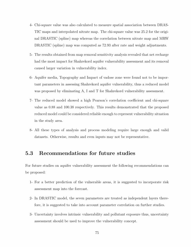
4- Chi-square value was also calculated to measure spatial association between DRAS-
TIC maps and interpolated nitrate map. The chi-square value was 25.2 for the origi-
nal DRASTIC (spline) map whereas the correlation between nitrate map and MRW
DRASTIC (spline) map was computed as 72.93 after rate and weight adjustments.
5- The results obtained from map removal sensitivity analysis revealed that net recharge
had the most impact for Shahrekord aquifer vulnerability assessment and its removal
caused larger variation in vulnerability index.
6- Aquifer media, Topography and Impact of vadose zone were found not to be impor-
tant parameters in assessing Shahrekord aquifer vulnerability, thus a reduced model
was proposed by eliminating A, I and T for Shahrekord vulnerability assessment.
7- The reduced model showed a high Pearson’s correlation coefficient and chi-square
value as 0.88 and 100.38 respectively. This results demonstrated that the proposed
reduced model could be considered reliable enough to represent vulnerability situation
in the study area.
8- All these types of analysis and process modeling require large enough and valid
datasets. Otherwise, results and even inputs may not be representative.
5.3 Recommendations for future studies
For future studies on aquifer vulnerability assessment the following recommendations can
be proposed:
1- For a better prediction of the vulnerable areas, it is suggested to incorporate risk
assessment map into the forecast.
2- In DRASTIC model, the seven parameters are treated as independent layers there-
fore, it is suggested to take into account parameter correlation on further studies.
3- Uncertainty involves intrinsic vulnerability and pollutant exposure thus, uncertainty
assessment should be used to improve the vulnerability concept.
75

References
[1] Soroush Abbasi, Kourosh Mohammadi, Majid Kholghi, and Ken Howard. Aquifer
vulnerability assessments using drastic, weights of evidence and the analytic element
method. Hydrological Sciences Journal, 58(1):186–197, 2013.
[2] Twana O Abdullah, Salahalddin S Ali, and Nadhir A Al-Ansari. Groundwater as-
sessment of halabja saidsadiq basin, kurdistan region, ne of iraq using vulnerability
mapping. Arabian Journal of Geosciences, 9(3):1–16, 2016.
[3] A Afshar, MA Marino, M Ebtehaj, and J Moosavi. Rule-based fuzzy system
for assessing groundwater vulnerability. Journal of Environmental Engineering,
133(5):532–540, 2007.
[4] U.S. EPA (Environmental Protection Agency). Drastic a standardized system for
the evaluating groundwater pollution using hydrogeologic settings. 1985.
[5] Rida AN Al-Adamat, Ian DL Foster, and Serwan MJ Baban. Groundwater vulner-
ability and risk mapping for the basaltic aquifer of the azraq basin of jordan using
gis, remote sensing and drastic. Applied Geography, 23(4):303–324, 2003.
[6] Akram Hassan Al Hallaq and Basheer Sofyan Abu Elaish. Assessment of aquifer
vulnerability to contamination in khanyounis governorate, gaza strippalestine, using
the drastic model within gis environment. Arabian Journal of Geosciences, 5(4):833–
847, 2012.
76

[7] Linda Aller, Jay H Lehr, Rebecca Petty, and Truman Bennett. Drastic: a
standhrdized system to evaluate ground water pollution potential using hydruged-
lugic settings, 1987.
[8] Manouchehr Amini, Karim C Abbaspour, Michael Berg, Lenny Winkel, Stephan J
Hug, Eduard Hoehn, Hong Yang, and C Annette Johnson. Statistical modeling
of global geogenic arsenic contamination in groundwater. Environmental science &
technology, 42(10):3669–3675, 2008.
[9] Manouchehr Amini, Kim Mueller, Karim C Abbaspour, Thomas Rosenberg, Majid
Afyuni, Klaus N Møller, Mamadou Sarr, and C Annette Johnson. Statistical model-
ing of global geogenic fluoride contamination in groundwaters. Environmental science
& technology, 42(10):3662–3668, 2008.
[10] AK Antonakos and NJ Lambrakis. Development and testing of three hybrid methods
for the assessment of aquifer vulnerability to nitrates, based on the drastic model,
an example from ne korinthia, greece. Journal of Hydrology, 333(2):288–304, 2007.
[11] Raheleh Arabgol, Majid Sartaj, and Keyvan Asghari. Predicting nitrate concen-
tration and its spatial distribution in groundwater resources using support vector
machines (svms) model. Environmental Modeling & Assessment, 21(1):71–82, 2016.
[12] Ronald G Aronovsky. Liability theories in contaminated groundwater litigation.
Environmental Forensics, 1(3):97–116, 2000.
[13] H Assaf and M Saadeh. Geostatistical assessment of groundwater nitrate contamina-
tion with reflection on drastic vulnerability assessment: the case of the upper litani
basin, lebanon. Water resources management, 23(4):775–796, 2009.
[14] Insaf S Babiker, Mohamed AA Mohamed, Tetsuya Hiyama, and Kikuo Kato. A gis-
based drastic model for assessing aquifer vulnerability in kakamigahara heights, gifu
prefecture, central japan. Science of the Total Environment, 345(1):127–140, 2005.
77

[15] Alan E Baker, James R Cichon, Jonathan D Arthur, and Gary L Raines. Florida
aquifer vulnerability assessment. In Geological Society of America Abstracts with
Programs, 2002.
[16] Jack E Barbash, Elizabeth A Resek, et al. Pesticides in ground water: distribution,
trends, and governing factors. Ann Arbor Press, 1996.
[17] C Barber, L Bates, R Barron, and H Allison. Assessment of the relative vulnerability
of groundwater to pollution: a review and background paper for the conference
workshop on vulnerability assessment. 1993.
[18] Rahim Barzegar, Asghar Asghari Moghaddam, and Hamed Baghban. A super-
vised committee machine artificial intelligent for improving drastic method to as-
sess groundwater contamination risk: a case study from tabriz plain aquifer, iran.
Stochastic environmental research and risk assessment, 30(3):883–899, 2016.
[19] Graeme F Bonham-Carter. Geographic information systems for geoscientists: mod-
elling with GIS, volume 13. Elsevier, 2014.
[20] LJ Brown, PN Dravid, NA Hudson, and CB Taylor. Sustainable groundwater
resources, heretaunga plains, hawke’s bay, new zealand. Hydrogeology Journal,
7(5):440–453, 1999.
[21] Michael R Burkart, Dana W Kolpin, Robert J Jaquis, and Kevin J Cole. Agrichemi-
cals in ground water of the midwestern usa: Relations to soil characteristics. Journal
of Environmental Quality, 28(6):1908–1915, 1999.
[22] TP Burt, ST Trudgill, AL Heathwaite, et al. Nitrate in groundwater. Nitrate:
processes, patterns and management., pages 213–238, 1993.
[23] Xavier Carreras, Josep Fraile, Teresa Garrido, and Carles Cardona. Groundwater
vulnerability mapping assessment using overlay and the drastic method in catalonia.
In Experiences from Ground, Coastal and Transitional Water Quality Monitoring,
pages 117–134. Springer, 2015.
78

[24] Mario Chica-Olmo, Juan Antonio Luque-Espinar, Victor Rodriguez-Galiano, Eulogio
Pardo-Iguzquiza, and Lucıa Chica-Rivas. Categorical indicator kriging for assessing
the risk of groundwater nitrate pollution: the case of vega de granada aquifer (se
spain). Science of the Total Environment, 470:229–239, 2014.
[25] M Civita. Le carte di vulnerabilita degli acquiferi allinquinamento: teoria e pratica.
Quaderni di tecniche di protezione ambientale, Pitagora ed, 1994.
[26] Massimo Civita, Marina De Maio, and F Berberi. Sintacs: un sistema parametrico
per la valutazione e la cartografia della vulnerabilita degli acquiferi all’inquinamento:
metodologia e automatizzazione. Pitagora Editrice, 1997.
[27] National Research Council. Ground Water Vulnerability Assessment: Predicting
Relative Contamination Potential Under Conditions of Uncertainty.
[28] Daly Daly, Alain Dassargues, Drew Drew, S Dunne, Nico Goldscheider, S Neale,
I Popescu, and Francois Zwahlen. Main concepts of the” european approach” to
karst-groundwater-vulnerability assessment and mapping. Hydrogeology Journal,
10(2):340–345, 2002.
[29] B Daneshfar and K Benn. Spatial relationships between natural seismicity and faults,
southeastern ontario and north-central new york state. Tectonophysics, 353(1):31–44,
2002.
[30] Gokhan Demir, Mustafa Aytekin, Aykut Akgun, Sabriye Banu Ikizler, and Orhan
Tatar. A comparison of landslide susceptibility mapping of the eastern part of the
north anatolian fault zone (turkey) by likelihood-frequency ratio and analytic hier-
archy process methods. Natural hazards, 65(3):1481–1506, 2013.
[31] Ferdinando Di Martino, Salvatore Sessa, and Vincenzo Loia. A fuzzy-based tool for
modelization and analysis of the vulnerability of aquifers: a case study. International
Journal of Approximate Reasoning, 38(1):99–111, 2005.
79

[32] Ali El-Naqa, Nezar Hammouri, and Mustafa Kuisi. Gis-based evaluation of ground-
water vulnerability in the russeifa area, jordan. Revista mexicana de ciencias
geologicas, 23(3):277–287, 2006.
[33] Bernard Engel, Kumar Navulur, Brian Cooper, and Leighanne Hahn. Estimating
groundwater vulnerability to nonpoint source pollution from nitrates and pesticides
on a regional scale. 1996.
[34] Babak Farjad, Helmi Zulhaidi bin Mohd Shafri, Thamer Ahmed Mohamed, Saied
Pirasteh, and Nishad Wijesekara. Groundwater intrinsic vulnerability and risk map-
ping. In Proceedings of the Institution of Civil Engineers-Water Management, volume
165, pages 441–450. Thomas Telford Ltd, 2012.
[35] Elham Fijani, Ata Allah Nadiri, Asghar Asghari Moghaddam, Frank T-C Tsai, and
Barnali Dixon. Optimization of drastic method by supervised committee machine
artificial intelligence to assess groundwater vulnerability for maragheh–bonab plain
aquifer, iran. Journal of hydrology, 503:89–100, 2013.
[36] Michael J Focazio, Dana W Kolpin, Kimberlee K Barnes, Edward T Furlong,
Michael T Meyer, Steven D Zaugg, Larry B Barber, and Michael E Thurman. A
national reconnaissance for pharmaceuticals and other organic wastewater contam-
inants in the united statesii) untreated drinking water sources. Science of the total
Environment, 402(2):201–216, 2008.
[37] SSD Foster. Fundamental concepts in aquifer vulnerability, pollution risk and pro-
tection strategy. Vulnerability of soil and groundwater to pollutants, 38:69–86, 1987.
[38] EO Frind, JW Molson, and DL Rudolph. Well vulnerability: a quantitative approach
for source water protection. Ground Water, 44(5):732–742, 2006.
[39] JD Pineros Garcet, Andre Ordonez, Jutta Roosen, and Marnik Vanclooster. Meta-
modelling: theory, concepts, and application to nitrate leaching. Developments in
Water Science, 55:915–924, 2004.
80

[40] NC Ghosh and RD Singh. Groundwater arsenic contamination in india: vulnerability
and scope for remedy. 2009.
[41] RC Gogu and Alain Dassargues. Current trends and future challenges in groundwater
vulnerability assessment using overlay and index methods. Environmental geology,
39(6):549–559, 2000.
[42] NICO Goldscheider, MARKUS Klute, Sebastian Sturm, and Heinz Hotzl. The pi
method–a gis-based approach to mapping groundwater vulnerability with special
consideration of karst aquifers. Z Angew Geol, 46(3):157–166, 2000.
[43] Balamurugan Guru, Karthik Seshan, and Somnath Bera. Frequency ratio model for
groundwater potential mapping and its sustainable management in cold desert, india.
Journal of King Saud University-Science, 2016.
[44] Hohberger KH Nachtigall KH Villinger E Weinzierl W. Hlting B, Haertle T. Concep-
tion for the evaluation of the protective function of the unsaturated stratum above
the groundwater table. Geol Jahrb.
[45] J Iqbal, AK Gorai, YB Katpatal, and G Pathak. Development of gis-based fuzzy
pattern recognition model (modified drastic model) for groundwater vulnerability to
pollution assessment. International Journal of Environmental Science and Technol-
ogy, 12(10):3161–3174, 2015.
[46] Jawed Iqbal, AK Gorai, Poonam Tirkey, and Gopal Pathak. Approaches to ground-
water vulnerability to pollution: a literature review. Asian Journal of Water, Envi-
ronment and Pollution, 9(1):105–115, 2012.
[47] Fatemeh Jafari, Saman Javadi, Golmar Golmohammadi, Kourosh Mohammadi, Ah-
mad Khodadadi, and Mohsen Mohammadzadeh. Groundwater risk mapping predic-
tion using mathematical modeling and the monte carlo technique. Environmental
Earth Sciences, 75(6):1–11, 2016.
[48] S Javadi, N Kavehkar, MH Mousavizadeh, and K Mohammadi. Modification of dras-
tic model to map groundwater vulnerability to pollution using nitrate measurements
81

in agricultural areas. Journal of Agricultural Science and Technology, 13:239–249,
2010.
[49] Saman Javadi, Neda Kavehkar, Kourosh Mohammadi, Ahmad Khodadadi, and Rene
Kahawita. Calibrating drastic using field measurements, sensitivity analysis and sta-
tistical methods to assess groundwater vulnerability. Water international, 36(6):719–
732, 2011.
[50] William A Jury and Masoud Ghodrati. Overview of organic chemical environmen-
tal fate and transport modeling approaches. Reactions and movement of organic
chemicals in soils, (reactionsandmov):271–304, 1989.
[51] Leon J Kauffman and Francis H Chapelle. Relative vulnerability of public supply
wells to voc contamination in hydrologically distinct regional aquifers. Groundwater
Monitoring & Remediation, 30(4):54–63, 2010.
[52] MC Kavanaugh. An overview of the management of contaminated sites in the us:
the conflict between technology and public policy. Water Science and Technology,
34(7-8):275–283, 1996.
[53] Leonard F Konikow and Eloise Kendy. Groundwater depletion: A global problem.
Hydrogeology Journal, 13(1):317–320, 2005.
[54] Masoome Arezoomand Omidi Langrudi, Abbas Khashei Siuki, Saman Javadi, and
Seyed Reza Hashemi. Evaluation of vulnerability of aquifers by improved fuzzy dras-
tic method: Case study: Aastane kochesfahan plain in iran. Ain Shams Engineering
Journal, 7(1):11–20, 2016.
[55] A Leone, MN Ripa, V Uricchio, J Deak, and Z Vargay. Vulnerability and risk
evaluation of agricultural nitrogen pollution for hungary’s main aquifer using drastic
and gleams models. Journal of Environmental Management, 90(10):2969–2978, 2009.
[56] Jin Li and Andrew D Heap. A review of spatial interpolation methods for environ-
mental scientists. 2008.
82
[57] Ruopu Li and James W Merchant. Modeling vulnerability of groundwater to pollu-
tion under future scenarios of climate change and biofuels-related land use change: A
case study in north dakota, usa. Science of the total environment, 447:32–45, 2013.
[58] Weldon A Lodwick, William Monson, and Larry Svoboda. Attribute error and sen-
sitivity analysis of map operations in geographical informations systems: suitability
analysis. International Journal of Geographical Information System, 4(4):413–428,
1990.
[59] Deepesh Machiwal, Madan K Jha, and Bimal C Mal. Gis-based assessment and
characterization of groundwater quality in a hard-rock hilly terrain of western india.
Environmental monitoring and assessment, 174(1-4):645–663, 2011.
[60] Alan Mair and Aly I El-Kadi. Logistic regression modeling to assess groundwater
vulnerability to contamination in hawaii, usa. Journal of contaminant hydrology,
153:1–23, 2013.
[61] A Margane. Guideline for groundwater vulnerability mapping and risk assessment
for the susceptibility of groundwater resources to contamination. bundesanstalt fur
geowissen schaften und rohstoffe (hannover, germany) archive no. 0122917, 2003.
[62] Jean Margat. Vulnerabilite des nappes deau souterraine a la pollution. BRGM
Publication, 68, 1968.
[63] M Masetti, S Poli, and S Sterlacchini. Aquifer vulnerability assessment using weights
of evidence modeling technique: application to the province of milan, northern italy.
In Proceedings of IAMG, pages 499–504, 2005.
[64] Marco Masetti, Simone Sterlacchini, Cristiano Ballabio, Alessandro Sorichetta, and
Simone Poli. Influence of threshold value in the use of statistical methods for ground-
water vulnerability assessment. Science of the total environment, 407(12):3836–3846,
2009.
83

[65] CDA McLay, R Dragten, G Sparling, and N Selvarajah. Predicting groundwater
nitrate concentrations in a region of mixed agricultural land use: a comparison of
three approaches. Environmental Pollution, 115(2):191–204, 2001.
[66] Yvonne J Meeks and J David Dean. Evaluating ground-water vulnerability to pesti-
cides. Journal of Water Resources Planning and Management, 116(5):693–707, 1990.
[67] M Metni, M EL-FADEL, S Sadek, R Kayal, and D Lichaa El Khoury. Groundwater
resources in lebanon: a vulnerability assessment. International Journal of Water
Resources Development, 20(4):475–492, 2004.
[68] Kourosh Mohammadi, Ramin Niknam, and Vahid J Majd. Aquifer vulnerability
assessment using gis and fuzzy system: a case study in tehran–karaj aquifer, iran.
Environmental geology, 58(2):437–446, 2009.
[69] Mohammadi,K. Groundwater flow and transport modeling of shahrkord aquifer.
Technical report, Charmahal-Bakhtyari, Provincial Water Authority, Shahrkord,
Iran, 2009.
[70] Majid Mohammady, Hamid Reza Pourghasemi, and Biswajeet Pradhan. Landslide
susceptibility mapping at golestan province, iran: a comparison between frequency
ratio, dempster–shafer, and weights-of-evidence models. Journal of Asian Earth
Sciences, 61:221–236, 2012.
[71] Seyed Amir Naghibi, Hamid Reza Pourghasemi, Zohre Sadat Pourtaghi, and Ashkan
Rezaei. Groundwater qanat potential mapping using frequency ratio and shannons
entropy models in the moghan watershed, iran. Earth Science Informatics, 8(1):171–
186, 2015.
[72] P Napolitano and AG Fabbri. Single-parameter sensitivity analysis for aquifer vulner-
ability assessment using drastic and sintacs. IAHS Publications-Series of Proceedings
and Reports-Intern Assoc Hydrological Sciences, 235:559–566, 1996.
84

[73] Aminreza Neshat and Biswajeet Pradhan. An integrated drastic model using fre-
quency ratio and two new hybrid methods for groundwater vulnerability assessment.
Natural Hazards, 76(1):543–563, 2015.
[74] Aminreza Neshat, Biswajeet Pradhan, and Mohsen Dadras. Groundwater vulnera-
bility assessment using an improved drastic method in gis. Resources, Conservation
and Recycling, 86:74–86, 2014.
[75] Aminreza Neshat, Biswajeet Pradhan, Saied Pirasteh, and Helmi Zulhaidi Mohd
Shafri. Estimating groundwater vulnerability to pollution using a modified dras-
tic model in the kerman agricultural area, iran. Environmental Earth Sciences,
71(7):3119–3131, 2014.
[76] Christoph Neukum and Rafig Azzam. Quantitative assessment of intrinsic groundwa-
ter vulnerability to contamination using numerical simulations. Science of the total
environment, 408(2):245–254, 2009.
[77] Bernard T Nolan, Kerie J Hitt, and Barbara C Ruddy. Probability of nitrate con-
tamination of recently recharged groundwaters in the conterminous united states.
Environmental science & technology, 36(10):2138–2145, 2002.
[78] World Health Organization. Guidelines for drinking-water quality: recommendations,
volume 1. World Health Organization, 2004.
[79] Issoufou Ouedraogo, Pierre Defourny, and Marnik Vanclooster. Mapping the ground-
water vulnerability for pollution at the pan african scale. Science of The Total En-
vironment, 544:939–953, 2016.
[80] FAL Pacheco, LMGR Pires, RMB Santos, and LF Sanches Fernandes. Factor weight-
ing in drastic modeling. Science of the Total Environment, 505:474–486, 2015.
[81] Fernando AL Pacheco and Luıs F Sanches Fernandes. The multivariate statistical
structure of drastic model. Journal of Hydrology, 476:442–459, 2013.
85

[82] GP Panagopoulos, AK Antonakos, and NJ Lambrakis. Optimization of the drastic
method for groundwater vulnerability assessment via the use of simple statistical
methods and gis. Hydrogeology Journal, 14(6):894–911, 2006.
[83] Eulogio Pardo-Iguzquiza, Mario Chica-Olmo, Juan A Luque-Espinar, and Vıctor
Rodrıguez-Galiano. Compositional cokriging for mapping the probability risk of
groundwater contamination by nitrates. Science of the Total Environment, 532:162–
175, 2015.
[84] CHRISTOPHER L Plymale and MP Angle. Groundwater pollution potential of
fulton county, ohio. Ohio Department of Natural resources division of water, water
resources section, Groundwater pollution potential report no, 45, 2002.
[85] PSC Rao, AG Hornsby, and RE Jesup. Indices for ranking the potential for pesti-
cide contamination of groundwater. In Proceedings Soil and Crop Science Society of
Florida, 1985.
[86] Lars Rosen. A study of the drastic methodology with emphasis on swedish conditions.
Ground Water, 32(2):278, 1994.
[87] Mahmood Sadat-Noori and Kumars Ebrahimi. Groundwater vulnerability assess-
ment in agricultural areas using a modified drastic model. Environmental monitoring
and assessment, 188(1):1–18, 2016.
[88] Satiprasad Sahoo, Anirban Dhar, Amlanjyoti Kar, and Durjoy Chakraborty. Index-
based groundwater vulnerability mapping using quantitative parameters. Environ-
mental Earth Sciences, 75(6):1–13, 2016.
[89] Erhan Sener and Aysen Davraz. Assessment of groundwater vulnerability based on a
modified drastic model, gis and an analytic hierarchy process (ahp) method: the case
of egirdir lake basin (isparta, turkey). Hydrogeology Journal, 21(3):701–714, 2013.
[90] MK Sinha, MK Verma, I Ahmad, K Baier, R Jha, and R Azzam. Assessment of
groundwater vulnerability using modified drastic model in kharun basin, chhattis-
garh, india. Arabian Journal of Geosciences, 9(2):1–22, 2016.
86

[91] Marc Soutter and Yvan Pannatier. Groundwater vulnerability to pesticide contami-
nation on a regional scale. Journal of Environmental Quality, 25(3):439–444, 1996.
[92] Dale Van Stempvoort, Lee Ewert, and Leonard Wassenaar. Aquifer vulnerability
index: a gis-compatible method for groundwater vulnerability mapping. Canadian
Water Resources Journal, 18(1):25–37, 1993.
[93] Roberto R Teso, Minn P Poe, Theodore Younglove, and Patrick M McCool. Use of
logistic regression and gis modeling to predict groundwater vulnerability to pesticides.
Journal of Environmental Quality, 25(3):425–432, 1996.
[94] D Thirumalaivasan, M Karmegam, and K Venugopal. Ahp-drastic: software for
specific aquifer vulnerability assessment using drastic model and gis. Environmental
Modelling & Software, 18(7):645–656, 2003.
[95] A Tiktak, JJTI Boesten, AMA Van der Linden, and Marnik Vanclooster. Mapping
ground water vulnerability to pesticide leaching with a process-based metamodel of
europearl. Journal of environmental quality, 35(4):1213–1226, 2006.
[96] John Troiano, Craig Nordmark, Terrell Barry, and Bruce Johnson. profiling ar-
eas of ground water contamination by pesticides in california: phase ii–evaluation
and modification of a statistical model. Environmental monitoring and assessment,
45(3):301–319, 1997.
[97] Zahrul Umar, Biswajeet Pradhan, Anuar Ahmad, Mustafa Neamah Jebur, and
Mahyat Shafapour Tehrany. Earthquake induced landslide susceptibility mapping
using an integrated ensemble frequency ratio and logistic regression models in west
sumatera province, indonesia. Catena, 118:124–135, 2014.
[98] Frank Wilcoxon. Individual comparisons by ranking methods. Biometrics bulletin,
1(6):80–83, 1945.
[99] Fred Worrall, Tim Besien, and Dana W Kolpin. Groundwater vulnerability: interac-
tions of chemical and site properties. Science of the Total Environment, 299(1):131–
143, 2002.
87
[100] Fred Worrall and Dana W Kolpin. Aquifer vulnerability to pesticide pollutioncom-
bining soil, land-use and aquifer properties with molecular descriptors. Journal of
Hydrology, 293(1):191–204, 2004.
[101] Ahmed M Youssef, Mohamed Al-Kathery, and Biswajeet Pradhan. Landslide sus-
ceptibility mapping at al-hasher area, jizan (saudi arabia) using gis-based frequency
ratio and index of entropy models. Geosciences Journal, 19(1):113–134, 2015.
[102] Ahmed M Youssef, Biswajeet Pradhan, and Elhami Tarabees. Integrated evalua-
tion of urban development suitability based on remote sensing and gis techniques:
contribution from the analytic hierarchy process. Arabian Journal of Geosciences,
4(3-4):463–473, 2011.
88


