This is a repository copy of Geographic information systems and perceptual dialectology: a method for processing draw-a-map data.
White Rose Research Online URL for this paper:http://eprints.whiterose.ac.uk/96521/
Version: Accepted Version
Article:
Montgomery, C. and Stoeckle, P. (2013) Geographic information systems and perceptual dialectology: a method for processing draw-a-map data. Journal of Linguistic Geography, 1(01). pp. 52-85. ISSN 2049-7547
https://doi.org/10.1017/jlg.2013.4
This article has been published in a revised form in Journal of Linguistic Geography [https://doi.org/10.1017/jlg.2013.4]. This version is free to view and download for private research and study only. Not for re-distribution, re-sale or use in derivative works. © Cambridge University Press 2013.
[email protected]://eprints.whiterose.ac.uk/
Reuse
This article is distributed under the terms of the Creative Commons Attribution-NonCommercial-NoDerivs (CC BY-NC-ND) licence. This licence only allows you to download this work and share it with others as long as you credit the authors, but you can’t change the article in any way or use it commercially. More information and the full terms of the licence here: https://creativecommons.org/licenses/
Takedown
If you consider content in White Rose Research Online to be in breach of UK law, please notify us by emailing [email protected] including the URL of the record and the reason for the withdrawal request.

1
Geographical Information Systems and Perceptual Dialectology: A method for processing draw-a-map data
Author details:
Chris Montgomery, Sheffield Hallam University, UK
Philipp Stoeckle, Albert-Ludwigs-Universität Freiburg, Germany
Lead author contact details:
Chris Montgomery
Department of Humanities
Faculty of Development and Society
Sheffield Hallam University
Sheffield
S1 1WB
Phone number: 0114 225 4473
Email: [email protected] / [email protected]
[please use both in correspondence, due to a new job, the Sheffield Hallam University address will expire at the
end of August 2012]
Short title:
GIS and Perceptual Dialectology

2
Abstract
This article presents a new method for processing data ェ;デエWヴWS ┌ゲキミェ デエW けSヴ;┘-a-マ;ヮげ デ;ゲニ (Preston 1982) in
Perceptual Dialectology (PD) studies. Such tasks produce large numbers of maps containing many lines indicating
non-ノキミェ┌キゲデゲげ ヮWヴIWヮデキラミゲ ラa デエW ノラI;デキラミ ;ミS W┝デWミデ ラa dialect areas. Although individual maps are interesting,
and numerical data relating to the relative prominence of dialect areas can be extracted, the real value of the
draw-a-map task is in aggregating data. This was always an aim of the contemporary PD method (Preston &
Howe 1987:363), although the nature of the data has meant that this has not always been possible. Here, we
argue for the use of Geographical Information Systems (GIS) in order to aggregate, process and display PD data.
Using case studies from the UK and Germany, we present examples of data processed using GIS, and illustrate
the future possibilities for the use of GIS in PD research.

3
1.0 Introduction
Aggregating data in perceptual dialectology is something which has occupied researchers since the earliest
research was undertaken in the field (Weijnen 1946; Mase 1999). Modern approaches to perceptual dialectology
┌ゲW マWデエラSゲ SWゲキェミWS デラ ;ゲゲWゲゲ ヴWゲヮラミSWミデゲげ マWミデ;ノ マ;ヮゲ ラa ノ;ミェ┌;ェW ┗;ヴキ;デキラミ ;ミS さSキェ SWWヮノ┞ キミデラ デエW
conceptual world, not only for the concepts of dialect areas but for the associated beliefs about speakers and
デエWキヴ ┗;ヴキWデキWゲざ (Preston 2010:11). Such methods, involving the use of hand-Sヴ;┘ミ マ;ヮゲ ふデWヴマWS けSヴ;┘-a-マ;ヮげ
tasks (Preston 1982)) have at their heart the aim of arriving at aggregate composite maps of dialect areas from
ヴWゲヮラミSWミデゲげ マ;ヮゲ (Preston & Howe 1987:363). Such aggregate maps can be used to give an account of where
respondents perceive dialect areas to exist, along with the extent of these areas. In this way, the methods of PD
extend our knowledge of speech communities (Kretzschmar 1999:xviii) by exploring the social space (Britain
2010:70) of these communities.
PD research can also play a role in looking afresh at the results of productions studies. Indeed, the ability of
the discipline to challenge assumptions made from such studies has been noted as one of its strengths (Butters
1991:296). In order to do this effectively, data must be aggregated in order to produce composite maps of
perceptual dialect areas. Perceptual geographers, who provided the impetus for contemporary approaches to
PD, knew this (see Gould & White 1986). The power of an aggregate is that it ェキ┗Wゲ ; ェWミWヴ;ノキゲWS けヮキIデ┌ヴWげ ラa
perception which has more explicative power than single images of mental maps produced by individual
respondents (cf. Lynch 1960; Orleans 1967; Goodey 1971).
Data from PD studies can be processed simply by counting the number of areas drawn on a number of maps
in order to arrive at the recognition level for each area. However, to stop at this stage as some have done (e.g.
Bucholtz et al. 2007) is to neglect much of the data supplied by respondents. This geographical data relating to
the placement and extent of dialect areas is a valuable resource that once properly processed can be used to
directly compare with data from other studies (linguistic and beyond).
Despite this, it is clear why some linguists have not attempted to produce aggregate maps. This is due to the
lack of a stable and useable method for completing this type of analysis for maps from large numbers of
respondents. This is in spite of デエキゲ HWキミェ ラミW ラa PヴWゲデラミげゲ ;キマゲ aラヴ PD (Preston & Howe 1987:363). In Bucholtz et
;ノげゲ (2007) study, for example, maps were drawn by 703 respondents. Processing and aggregating data from

4
such a large number of respondents is simply not possible given that the most widely available technique is line
tracing using overhead transparencies (see Montgomery 2007:61に68)i).
In order to work with maps from large numbers of respondents there is a need for an up-to-date, portable,
accessible, computerised method of processing and aggregating PD data. Attempts at creating such a method
have been made in the past. The first was made by Preston and Howe (1987), who developed a technique
involving the use of a digitising pad and bespoke software. This allowed the storage of digitised line information
relating to a dialect area, along with the demographic data of the respondent who drew it. Many lines could be
traced using the digitising pad with the result that aggregate maps of the dialect area could be displayed. These
areas could also be queried on the basis of the demographic information. A map created using Preston and
Hラ┘Wげゲ デWIエミキケ┌W I;ミ HW ゲWWミ キミ Fキェ┌ヴW ヱく
INSERT FIGURE 1 HERE
PヴWゲデラミ ;ミS Hラ┘Wげゲ (1987) method ensured that there was a method for producing aggregate maps which
also meant that they would be able to be queried. This is a major advantage over a non-computerised
technique, as it did not require separate aggregation techniques for each social variable one wished to examine.
This approach was built upon by Onishi and Long (1997) ;ゲ デエW┞ ┌ヮS;デWS PヴWゲデラミ ;ミS Hラ┘Wげゲ (1987) technique
for use with Windows computers. The resulting software, entitled Perceptual Dialectology Quantifier for
Windows (PDQ), processed data in the same way as Preston aミS Hラ┘Wげゲ (1987) technique. A digitising pad was
again used to input area line data, and the software package did the rest of the data processing. Figure 2 shows
an aggregate map produced using PDQ.
INSERT FIGURE 2 HERE
Although the methods developed by Preston and Howe (1987) and Onishi and Long (1997) made working
with draw-a-map data easier, there were problems with their approaches. The most pressing problem was the
ノ;Iニ ラa けa┌デ┌ヴW ヮヴララaキミェげ H┌キノデ キミデラ デエW デWIエミラノラェ┞く TエW デWIエミラノラェ┞ ┌ゲWS H┞ PヴWゲデラn and Howe (1987) quickly
became obsolete, as did the technology used by Onishi and Long (1997). Thus, although PDQ for Windows is still
5
functional to some extent, there are major problems with it. It is not portable and is only available for use in
Japan (running on three increasingly elderly computers). A second issue is the low resolution of the maps
produced by the programme (as can be seen in Figure 2), which renders them less suitable for publication. A
third problem is the way in which the programme permits the display of only one area on a map, which makes it
unsuitable for producing composite maps showing multiple perceptual areas on one map (i.e. Preston
1999a:362).
More recent studies (e.g. Purschke 2011) have used simple overlay techniques in vector (cf. section 3.1)
graphics programmes (such as CorelDraw, Adobe Illustrator, etc.). Such programmes can yield quite impressive
results and an example can be seen in Figure 3, which shows a summary of subjective dialect areas in Germany
drawn by informants from Northern (left map) and Eastern (right map) Hessian informants.
INSERT FIGURE 3 HERE
The different colours in Figure 3 indicate aggregate perceptions of different dialect areas, and the colour
densities show different degrees of agreement. This method clearly improves on the quality of visualisation, and
the researcher is able to get an impression of which dialect areas are the most prominent and where they are
located. However, the use of this type of technology does not allow any further analyses such as the exact
calculation of agreement levels, area sizes, or distances (e.g. to the next political border). Also, due to an
キミ;Hキノキデ┞ デラ け;ミIエラヴげ デエW ┗キゲ┌;ノキゲ;デキラミ キミ デエW ヴW;ノ ┘ラヴノS ふIaく ゲWIデキラミ ンくヲぶが キデ キゲ SキaaキI┌ノデ デラ マWヴェW PD S;デ; ┘キth other
kinds of data sets (such as streets, topography, etc.).
Given the difficulty of processing and aggregating geographical data from draw-a-map tasks without the use
of a computer, and the general insufficiency of useable computerized techniques, there is a pressing need for
new technology which can be used in this area. In this article we discuss the role Geographical Information
Systems (GIS) may play in filling the gap.
After a short review of the use of the draw-a-map task in PD (section 1.1) we will introduce the surveys and
methods of data collection our analyses are based on (section 2). Following that, the principles of GIS will be
presented and how they can be applied to PD data discussed (section 3). We will then demonstrate some

6
examples of the possibilities of GIS to visualize and analyse geospatial data (section 4) before summarizing our
findings and arguing for a more extensive use of this technology (section 5).
1.1 The draw-a-map task in Perceptual Dialectology
One of the aims of PD research, as mentioned above, is to assess where respondents believe dialect areas to
exist (Preston 1988:475に6). The technique used to investigate this is the draw-a-map task (Preston 1982).
Respondents undertaking the task are asked to "'dra┘ Hラ┌ミS;ヴキWゲ ラミ ; ぐ マ;ヮ ;ヴラ┌ミS ;ヴW;ゲ ┘エWヴW デエW┞ HWノキW┗W
regional speech zones [to] exist" (Preston 1999b:xxxiv). An example of a completed draw-a-map task, from one
of the studies considered here, can be seen in Figure 4.
INSERT FIGURE 4 HERE
Data gathered the task has a twofold usefulness (Garrett 2010:183): "Firstly, it provides some insight into
┘エ;デ ;ミS ┘エWヴW Sキ;ノWIデ ヴWェキラミゲ ;Iデ┌;ノノ┞ W┝キゲデ キミ ヮWラヮノWろゲ マキミSゲ ぐ “WIラミSノ┞が デエW デ;ゲニ ェWミWヴ;デWゲ ;デデキデ┌Sキミ;ノ
comment alongside more descriptive data". We are interested in this article in the first use of the data (the
spatial aspect). We focus on how we might best process these data in order that we can better understand what
respondents think of regional variation, as well as "how concentrated or extensive" (Garrett 2010:183)
respondents think dialect regions are.
The draw-a-map task has been used in very large countries such as the United States (e.g. Preston 1986) and
Canada (McKinnie & Dailey-OげC;キミ ヲヰヰヲぶ, as well as in individual states (Bucholtz et al. 2007; Bucholtz et al.
2008; Anders 2010; Evans 2011) and smaller countries (Long 1999; Montgomery 2007). Whilst this PD research is
interested mainly in the question of how non-linguists classify large-scale dialect areas, other studies focus on
デエW ゲ┌HテWIデキ┗W Iラミゲデヴ┌Iデキラミ ラa ノラI;ノ Sキ;ノWIデ ;ヴW;ゲ キミ デエW ゲヮW;ニWヴゲげ キママWSキ;デW ミWキェエHラ┌ヴエララSく Q┌Wゲデキラミゲ ラa デエキゲ
kind were especially of interest in the early years of PD (see studies conducted in the Netherlands (Weijnen
1946) or in Japan (Mase 1999; Sibata 1999)). Indeed, the draw-a-map task is based on those used by perceptual
geographers in both small and large areas (see Gould and White (1986) for more discussion of such methods).

7
This paper uses data from two studies which took different approaches to the investigation of the perception
of language variation. The first (Study 1ii) is a large-ゲI;ノW ゲ┌ヴ┗W┞が ┘エラゲW ;キマ ┘;ゲ デラ ノララニ ;デ デエW ミ;デキラミ;ノ けヮキIデ┌ヴWげ
of language variation. The second (Study 2iii) took a small-scale approach, with the aim of investigating local
perceptions of variation. In the next section we discuss the datasets we will consider in this article.
2.0 Methods
The two studies considered here used the draw-a-map task. Both gathered data in Europe, although in
different countries, and therefore investigate perceptions of variation in different languages. Study 1
investigated the large-scale perceptions of dialects in Great Britain. The data presented from Study 2 deal with
the subjective construction of local dialect areas in the southwest of Germany as well as in some places in
Switzerland and in France (for first results see Stoeckle (2010; 2011)). Figure 4 shows a completed hand-drawn
map from Study 1, whilst Figure 5 shows dialect areas drawn by a respondent from Study 2.
INSERT FIGURE 5 HERE
Study 1 took a large-ゲI;ノW ;ヮヮヴラ;Iエが ┘キデエ デエW ;キマ ラa ェ;デエWヴキミェ S;デ; ヴWノ;デキミェ デラ デエW ミ;デキラミ;ノ けヮキIデ┌ヴWげ ラa
perception in Great Britain from five survey locations around the Scottish-English border. In this way, the study
aimed to investigate the impact of the Scottish-English border on the perception of language variation in English
(see Montgomery Forthcoming). Figure 6 shows each of the survey locations and the survey area (Scotland,
Wales, and England).
INSERT FIGURE 6 HERE
Respondents in Study 1 were given a minimally detailed map containing country borders and some city
location dotsiv. In all locations, they were asked to complete the paper map with a pen or pencil by in the
following fashion:

8
1) Label the nine well-known cites marked with a dot on the map.
2) Do you think that there is a north-south language divide in the country?v If so, draw a line where you think
this is.
3) Draw lines on the map where you think there are regional speech (dialect) areas.
4) Label the different areas that you have drawn on the map.
5) Wエ;デ Sラ ┞ラ┌ デエキミニ ラa デエW ;ヴW;ゲ ┞ラ┌げ┗W テ┌ゲデ Sヴ;┘ミい Hラ┘ マキェエデ ┞ラ┌ ヴWIラェミキゲW ヮWラヮノW aヴラマ デエWゲW ;ヴW;ゲい
Write some of these thoughts on the map if you have time.
A location map which contained a number of cities and towns in England, Scotland and Wales was projected
for respondents (who completed the task as part of a class) for the first five minutes of the task, which lasted for
10 minutes overall. 151 respondents in total completed the fieldwork, 76 on the Scottish side of the border, and
75 on the English side. The mean age of the respondents was 16 years and 6 months. Respondents drew 970
lines delimiting 79 separate areas (an average of 6.4 areas drawn per map).
Study 2 is a small-scale survey dealing with the question of how non-linguists construct dialect areas on a
local level. The data collection took place in the southwest of Germany as well as in some places in France and in
Switzerland. Figure 7 gives an overview of research area and the 37 investigated locations.
INSERT FIGURE 7 HERE
As demonstrated in Figure 7, 32 survey locations are found in Germany, three in Alsace (France) and two in
Switzerland. It was the aim in each location to interview six respondents, differentiated by the socio-
demographic variables of age, sex, and profession. In some locations it was not possible to find speakers for all
categories, and the total number of interviews was therefore 218 (instead of 222, the number originally aimed
for).
As part of the interview, respondents were asked to complete a draw-a-map task where they were given a
map and asked to draw:

9
1) their own local dialect area, and
2) all other surrounding dialect areas they knew of
Once they had completed the initial taskvi, the map served as a starting point for further characterisations of
the dialect areas. These concerned:
3) dialect features or stereotypes
4) ゲキマキノ;ヴキデキWゲっSキaaWヴWミIWゲ ┘キデエ ヴWェ;ヴS デラ デエW ヴWゲヮラミSWミデゲげ ラ┘ミ Sキ;ノWIデ
5) evaluations of the dialectality degrees of the identified areas and
6) judgements about the most (and least) pleasant dialects
The data generated in the interviews were subject to both qualitative and quantitative analyses. In this paper
we will focus on the latter.
Studies 1 and 2 take slightly different approaches to the study of large- and small-scale perceptions. However,
their similar use of a draw-a-map task in order to gather spatial data relating to the mental maps of dialect area
boundaries (seen in Figures 3 and 4) means that although the cognitive concepts may differ in each case, the
data generated in both types of research are very similar and thus require the same type of digital processing.
3.0 What is a GIS, what does it do, and why should we use one?
In the following we present some characteristics of a Geographical Information System (GIS). Since these
systems are very complex in nature, the literature contains many different approaches to the topic. Some deal
with detailed explanations of the workings of the technology whilst others discuss specific aspects and tools
provided by it. We wish to give a more basic outline here, focussing on what a GIS is and what it can be used for
in relation to PD work.
A GI“ キゲ SWaキミWS ;ゲ ; ゲ┞ゲデWマ ┘エキIエ キミデWェヴ;デWゲ デエW デエヴWW H;ゲキI WノWマWミデゲ ラa エ;ヴS┘;ヴWが ゲラaデ┘;ヴWが ;ミS S;デ; さaラヴ
capturing, man;ェキミェが ;ミ;ノ┞ゲキミェが ;ミS Sキゲヮノ;┞キミェ ;ノノ aラヴマゲ ラa ェWラェヴ;ヮエキI;ノノ┞ ヴWaWヴWミIWS キミaラヴマ;デキラミざ (ESRI 2011b).
In this article we use ArcGISvii (cf. Evans 2011) to process and display our data, although we will attempt to

10
explain the steps undertaken in for data processing in a general fashion so that they can be adapted for other
types of GIS software.
The main way in which a GIS works is by combining different types of data (see section 3.1) by linking them to
デエW W;ヴデエげゲ ゲ┌ヴa;IWく Tエキゲ デWIエミキケ┌W キゲ デWヴマWS けェWラヴWaWヴWミIキミェげ ;ミS キデ ヮWヴマキデゲ ; GI“ デラ さIラマHキミW ゲWマ;ミデキI ;ミS
ェWラマWデヴキI;ノ キミaラヴマ;デキラミざ (Gomarasca 2009:481). Georeferencing uses coordinate systems in order to tie data to
; ゲWデ ヮラゲキデキラミ ラミ デエW W;ヴデエげゲ ゲ┌ヴa;IWく Iデ キゲ キマヮラヴデ;ミデ エラ┘W┗Wヴ デラ ミラデW デエ;デが S┌W デラ ゲヮエWヴラid nature of the earth,
assigning a single coordinate system to the whole of the globe is fraught with difficulties. As a result of this,
SキaaWヴWミデ IララヴSキミ;デW ゲ┞ゲデWマゲ ふラヴ ヮヴラテWIデキラミゲぶ ;ヴW ┌ゲWS SWヮWミSキミェ ラミ デエW ┌ゲWヴげゲ ヮラゲキデキラミ ラミ デエW ェノラHWく Tエキゲ I;ミ
cause some confusion for users of GIS programmes, although in most cases the national grid projection of the
┌ゲWヴゲげ エラマW Iラ┌ミデヴ┞ ゲエラ┌ノS HW キミ ェWラヴWaWヴWミIキミェく WW SキゲI┌ゲゲ ェWラヴWaWヴWミIキミェ キミ ヴWノ;デキラミ デラ PD S;デ; キミ マラヴW
detail below.
Once data has been georeferenced, a GIS offers many possibilities for advanced data processing (known as
けェWラヮヴラIWゲゲキミェげぶく M;ミ┞ ェWラヮヴラIWゲゲキミェ デララノゲ ;ヴW SWゲキェミWS aラヴ IラママWヴIキ;ノ ラヴ Wミ┗キヴラミマWミデ;ノ WミSゲが ;ノデエラ┌ェエ デエW┞
can also be used for other purposes such as working with linguistic data. In addition to various possibilities
offered by geoprocessing tools a GIS also provides different ways of visualizing data or creating maps. Thus,
maps are georeferenced and therefore spatially meaningful, unlike conventional maps which contain only visual
information (i.e. they consist of pixels of different colours). Moreover, all geographical data can have or be
linked to many different types of attributes (metrical, numerical, descriptive, complex (cf. Gomarasca
2009:484)).
In summary, a GIS enaHノWゲ ; ┌ゲWヴ デラ ヮヴラIWゲゲが ;ミ;ノ┞ゲW ;ミS ┗キゲ┌;ノキ┣W ;ノノ ニキミSゲ ラa マラSWノゲ ラa デエW W;ヴデエげゲ ゲ┌ヴa;IWく
This makes the technology attractive not only for geographers and geologists, but also for researchers of other
disciplines (like archaeology, forestry, architecture, or civil engineering) as well as administrative applications
(like urban planning or traffic control) (Saurer & Behr 1997:10). In (perceptual) dialectology however, such
technologies have been used very rarely so far (exceptions being Kirk and Kretzschmar (1992), Labov, Ash and
Boberg (2006), Lameli et al (2008), and Evans (2011)). This is despite the fact that dialectological questions and
problems are by definition related to geographical space. Generally speaking, much simpler technologies have
been ┌ゲWS デラ IヴW;デW マ;ヮゲが デエW ;キマゲ ラa ┘エキIエ ┘WヴW ミラデ ミWIWゲゲ;ヴキノ┞ さspatially sensitiveざ (Britain 2009:144).

11
In dialect production studies, all necessary geographical information is selected by the researcher in advance
(e.g. the survey locations). GeographiI;ノ ゲヮ;IW デエWミ ゲWヴ┗Wゲ ;ゲ ; デWマヮノ;デW ふラヴ さHノ;ミニ I;ミ┗;ゲゲざ (Britain 2009:144))
onto which different linguistic features can be assigned to predefined places. In PD, however, geographical data
do not only serve as background. They also present the object of study as they are the data given by the
respondents though their completion of hand-drawn maps. The enormous advantage of GIS lies in its ability to
process, analyse and visualize these data and to combine them with reference to other geography-related data
such as topography, political boundaries, population statistics or dialect isoglosses (cf. section 4.1).
3.1 How a GIS works with data
Cラマヮ┌デWヴゲ さヴWケ┌キヴW ┌ミ;マHキェ┌ラ┌ゲ キミゲデヴ┌Iデキラミゲ ラミ エラ┘ デラ デ┌ヴミ S;デ; ;Hラ┌デ ゲヮ;デキ;ノ WミデキデキWゲ キミデラ ェWラェヴ;ヮエキI;ノ
ヴWヮヴWゲWミデ;デキラミゲざ (Heywood, Cornelius, & Carver 2006:77) and as a result a GIS works with data in specific ways.
Understanding the different ways in which a GIS deals with data from the real world is important if we wish to
use the technology to process data from PD (Heywood et al. 2006:77).
A GI“ ┘ラヴニゲ ┘キデエ S;デ; キミ けノ;┞Wヴゲげが ラ┗Wヴノ;┞キミェ デエWマ キミ ラヴSWヴ デラ ヮヴラS┌IW IラマヮラゲキデW マ;ヮゲく TエWゲW ノ;┞Wヴゲ ラa Sata
can be queried and manipulated, and the relationships between them investigated. This makes GIS technology
particularly attractive for multi-layered data such as that gathered in PD research. A GIS works with different
types of data, and we wish to dra┘ ヴW;SWヴゲげ ;デデWミデキラミ デラ デエW SキゲデキミIデキラミ HWデ┘WWミ デエW デ┘ラ ヮヴキマ;ヴ┞ デ┞ヮWゲ ラa
(spatial) data: raster data, and vector data.
Raster data can be imagined as a grid, or as consisting of cells. Each of these cells has a certain value which is
さマキヴヴラヴWS H┞ ;ミ Wケ┌キ┗;ノWミデ ヴラ┘ ラa ミ┌マHWヴゲ キミ デエW aキノW ゲデヴ┌Iデ┌ヴWざ (Heywood et al. 2006:79). A real-world object
マ;ヮヮWS ;ゲ ; ヴ;ゲデWヴ ┘キノノ デエWヴWaラヴW けaキノノげ ゲラマW ラa デエW IWノノゲ キミ デエW ェヴキSが ┘エキIエ ┘キノノ IラヴヴWゲヮラミS デラ キデゲ ゲエ;ヮW キミ デエW ヴW;ノ
world. The way in which raster data is stored by a GIS means that attribute data cannot be attached to it (see
below), which limits its usefulness if a user wishes to query the data at a later stage.
Vector data use co-ordinates to map real world objects, as opposed to the grid and cell method used by raster
datasets. The file structure of a vector dataset is a series of co-ordinate points. These points can be connected in
order to form lines or polygons. Unlike areas in raster datasets there is no information stored about surface

12
characteristics (so, the individual points within an area). Attribute data can be added to vector data. Figure 8
shows the different way in which vector and raster data are represented in a GIS.
INSERT FIGURE 8 HERE
Attribute data are a third type of data (Nash Parker & Asencio 2008:xvi), and they are also important for GIS
processing. This data type provides descriptive information linked to the map data by the GIS. It can contain
information about the name of an individual piece of the map data, for example, but can also contain a good
deal more information about the map data (such as population size, statistical information etc.). We will
demonstrate the use of both raster and vector datasets in this article, along with attribute data, which assists in
querying processed data.
3.2 General steps involved in processing data from hand-drawn maps
The steps involved in processing data from hand-drawn maps described below do not differ significantly from
those used by Preston and Howe (1987) or Onishi and Long (1997). Data relating to dialect areas still need to be
extracted from maps, attribute data (in the form of demographic information) added, and the data processed.
Only then can aggregate maps of dialect areas be displayed. The ArcGIS-based method we detail below follows
these steps relatively closely, although it does not use technology designed specifically for the task. This means
that what we describe can at first seem daunting, however the advantage of using a widely used and available
けラaa-the-ゲエWノaげ ヮrogramme will be demonstrated as we proceed.
Although a complete account of every data processing stage will not be possible here for reasons of space. It
is worth noting at this point that the instructions below will require some basic familiarity with the ArcGIS
environment (or the equivalent environment of the GIS you wish to use). This cannot be conveyed here,
although there are several useful resources available online and elsewhere.viii We should also emphasise that the
HWミWaキデゲ ラa けヮキIニキミェ ┌ヮけ デWIエniques by using the software should not be underestimated.
As we discuss above, the essential characteristic of a GIS is that it enables users to work with data which are
georeferenced. The first data processing stage is therefore to scan all of the hand-drawn maps and to add them

13
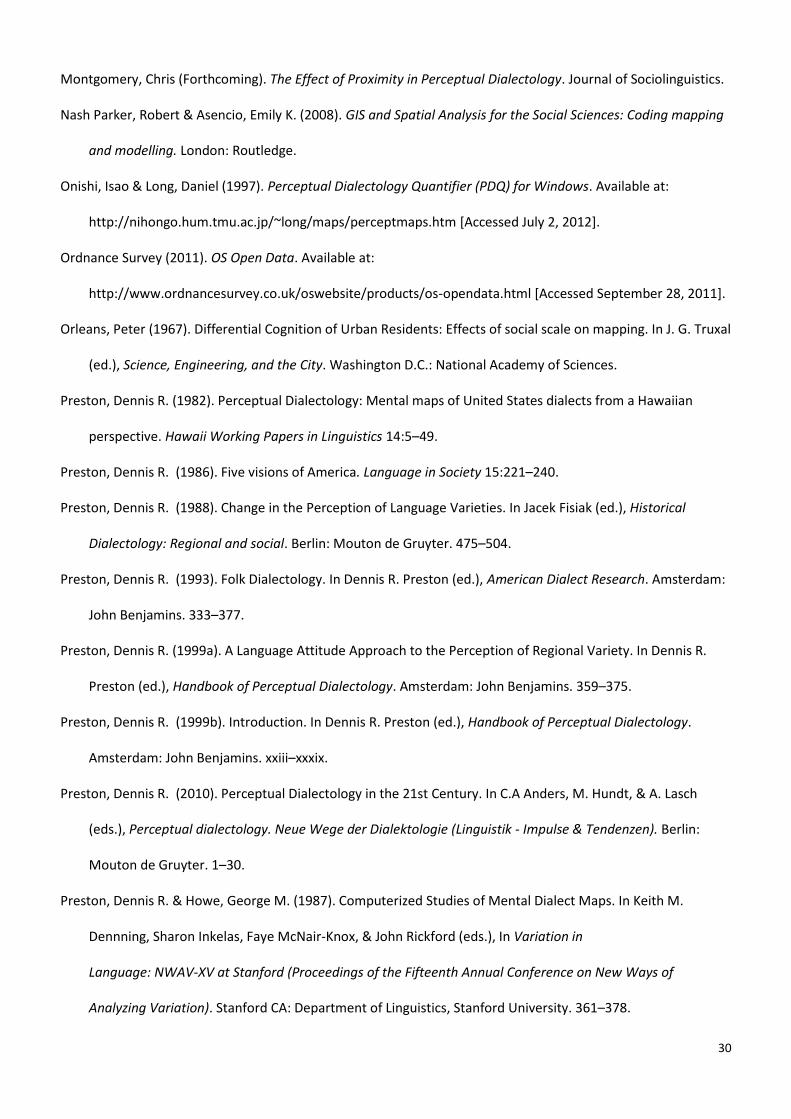
デラ ;ミ AヴIGI“ けヮヴラテWIデげ ふデエW デWヴマ デエW ヮヴラェヴ;ママW ェキ┗Wゲ デラ マ;ヮ SラI┌マWミデゲぶく GWラヴWaWヴWミIキミェ I;ミ デエWミ HW SラミW
┌ゲキミェ デエW さGWラヴWaWヴWミIキミェざ デララノ H┞ ;SSキミェ けIラミデヴラノ ヮラキミデゲげく けCラミデヴラノ ヮラキミデゲげ ;ヴW ヮラキミデゲ デエ;デ エ;┗W HWWミ ゲWノWIデWS
on a map which can be aligned with known points on another map. This means that if there is no information
;Hラ┌デ ; マ;ヮげゲ IララヴSキミ;デW ゲ┞ゲデWマが キデ I;ミ HW ェWラヴWaWヴWミIWS H┞ ┌ゲキミェ W┝キゲデキミェ S;デ; ふゲ┌Iエ ;ゲ HラヴSWヴゲが ヴキ┗Wヴゲ WデIくぶ ;ゲ
reference points which can be associated with the map with the help of the control points. Figure 9 shows the
principal behind georeferencing, in which three control points have been identified.
INSERT FIGURE 9 HERE
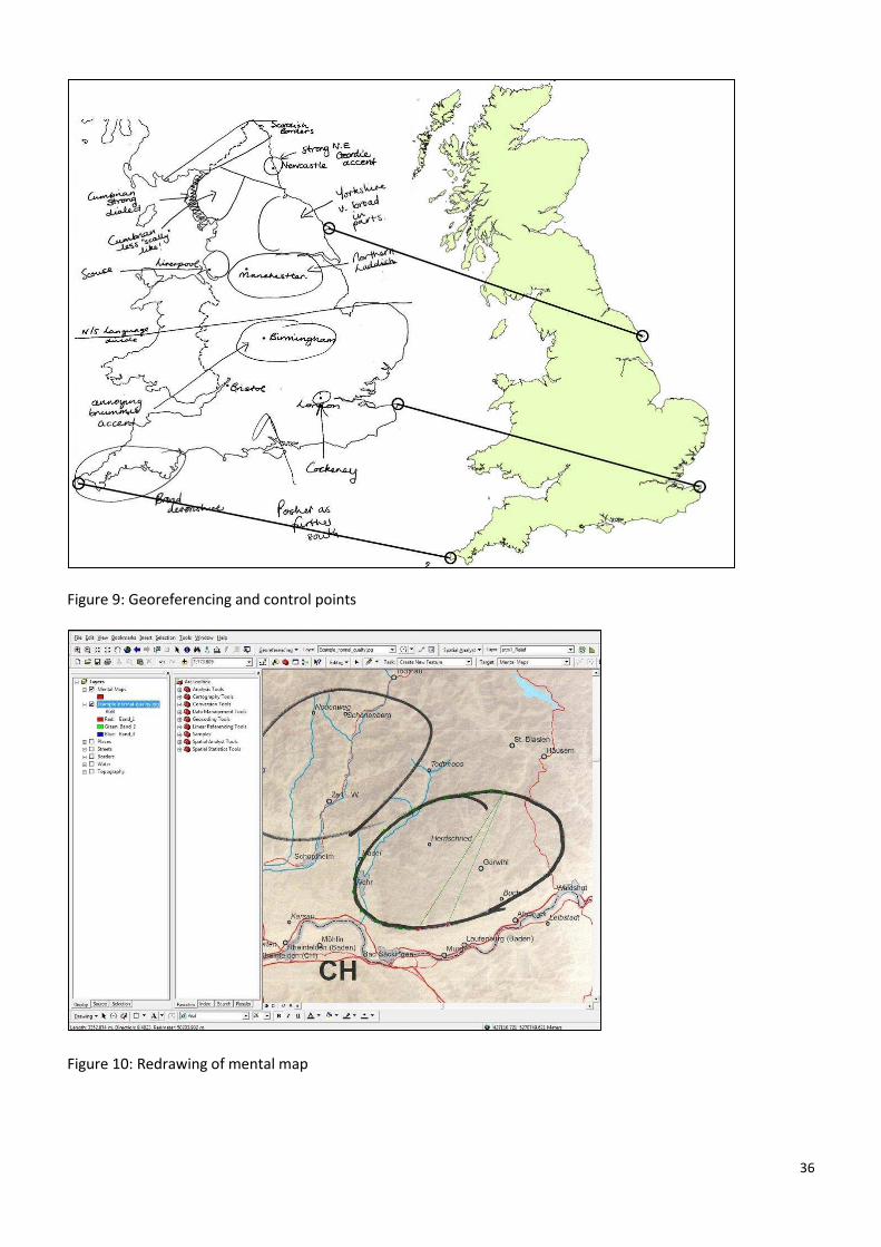
The remainder of this section will use data from Study 2, in order that a clear work flow can be observed.
Figure 10 shows a sample of a map from this study which has been scanned, added to an ArcGIS project, and
then georeferenced.
INSERT FIGURE 10 HERE
Once the map is georeferenced, the dialect areas drawn by the respondents must be digitized. In ArcGIS this
can be managed by creating a polygon feature class (a vector data type (cf. 3.2)). After the creation of the
polygon feature class, a file is created which as yet contains no data. Slots for attribute data can be created
during this step, which will allow the user to input further data (such as demographic or attitudinal data) at a
later stage.
Iミ ラヴSWヴ デラ ヮラヮ┌ノ;デW デエW ミW┘ ヮラノ┞ェラミ aW;デ┌ヴW Iノ;ゲゲが デエW さESキデラヴざ デララノ キゲ ゲデ;ヴデWS ;ミS デエW デララノ さCヴW;デW NW┘
FW;デ┌ヴWざ ┌ゲWSく This permits the dialect area indicated on the hand drawn map to be entered into the feature
S;デ; ゲWデ ふエWヴW ミ;マWS さMWミデ;ノ M;ヮゲざぶ H┞ デヴ;Iキミェ ;ヴラ┌ミS キデく Aゲ ┘W エ;┗W SキゲI┌ゲゲWS ;Hラ┗Wが ヴWゲヮラミSWミデゲ キミ Hラデエ
studies were not only asked to draw maps, but were also requested to label the areas and to evaluate them
according to different aspects (cf. section 2). GIS offers the possibilities to add any kind of attributes to the data
sets (cf. section 4.1). In the case of Study 2, attributes relating to the respondents (place of origin, sex, age) and
14
the dialect area (name of dialect area, characteristics) were added to the attribute table. Figure 11 shows both
the redrawn dialect area as well as the table containing different attributes relating to itix.
INSERT FIGURE 11 HERE
The next stage of the processing method is the hand-drawn map aggregation. The first step of this process
involves adding every redrawn area to one data set (using the same process as described above). Figure 12
shows the same dataset as in Figure 11, but now containing six different polygons (each representing
perceptions of the same dialect area drawn by six different respondents) with their respective attributes in the
table.
INSERT FIGURE 12 HERE
Up to this point, the different polygons are stored in one data set and as a result it is not possible to show
different degrees of agreement, which is one of the aims of the method. This can be achieved by a two-stage
process: first the self-union of the feature class containing all the polygons has to be calculated (by using the
さUミキラミざ デララノぶが ;ミS デエWミ デエW aヴWケ┌WミI┞ ラa W;Iエ ラa デエW ヮラノ┞ェラミゲ キミ デエW ラ┌デヮ┌デ エ;ゲ デラ HW Iラ┌ミデWS ふH┞ ┌ゲキミェ デエW
さFヴWケ┌WミI┞ざ デララノぶ ;ミS デエW ラ┌デヮ┌デ ラa デエキゲ I;ノI┌ノ;デキラミ ;SSWS デラ デエW map. The frequency count of all the polygons,
in this case ranging from one to six, gives the different degrees of overlap. Figure 13 shows a possible
visualisation as a result of this process.
INSERT FIGURE 13 HERE
Above, we have outlined the steps which will produce a basic map displaying agreement about the placement
and extent of a dialect area amongst a group of respondents. Data processing should not stop here however as
this type of dataset (i.e. vector data) requires a large amount of memory space and is thus hard to handle.
Secondly, it is difficult to either merge the dataset with other kinds of data sets (e.g. more polygons indicating a

15
dialect area, or neighbouring regions) or to perform further analyses on it. Thirdly, it displays all of the single
values of overlap, which results in too much influence from single areas and many sharp borders. Conversion
from vector to raster data is therefore helpfulx as this data format permits these types of processing.
The process outlined below requires the use of a large dataset in order that the benefits become most
apparent. To this end we have used data from Study 2 relating to the so-I;ノノWS けK;キゲWヴゲデ┌エノげ ぷノキデWヴ;ノノ┞ WマヮWヴラヴげゲ
chair], a small mountain and former volcano very close to the French border which is very well known for its
viticulture. This was the most readily recognised area amongst respondents in Study 2. Of the total of 218
respondents, 95 identified and drew this area. Using the same stage of the data processing technique as shown
キミ Fキェ┌ヴW ヱンが Fキェ┌ヴW ヱヴ ゲエラ┘ゲ デエW ヮWヴIWキ┗WS けK;キゲWヴゲデ┌エノげ Sキ;ノWIデ ;ヴW;く Fラヴ Iラマヮ;ヴキゲラミが Fキェ┌ヴW ヱヵ ゲエラ┘ゲ ; ヴ;ゲデWヴ-
based map of the perception of the same area.
INSERT FIGURE 14 HERE
INSERT FIGURE 15 HERE
Although containing the same data, the raster data set shown in Figure 15 gives a much better impression of
ヴWゲヮラミSWミデゲげ ヮWヴIWヮデキラミ ラa デエW けK;キゲWヴゲデ┌エノげ Sキ;ノWIデ ;ヴW; デエ;ミ デエ;デ Sキゲヮノ;┞WS キミ Fキェ┌ヴW ヱヴく TエW さNWキェエHラ┌ヴエララS
“デ;デキゲデキIゲざ デララノ エ;ゲ HWWミ ┌ゲWS キミ Fキェ┌ヴW ヱヵ キミ ラヴSWヴ デラ ゲマララデエ デエW ゲ┌ヴa;IW ラa デエe data, which makes any sharp
edges between the different degrees of overlap disappear. A continuous scale has been used with contour lines
added. The contour lines (unlike in topographic maps) do not indicate altitude, but degree of overlap.
The data processing technique described above can be summarised as the flow chart shown in Figure 16xi.
INSERT FIGURE 16 HERE
There is no doubt that, in addition to improving the processing and display of PD data, the use of GIS has
numerous advantages over the other processing techniques discussed above. Chief amongst these is the ability
to make PD data more useable alongside other datasets. Other advantages include the customisation of

16
aggregate data, the ability to combine individual areas on the same map, as well as the numerous possibilities to
perform calculations and statistical analyses on the data. We will discuss this in more detail in the next section.
4.0 Merging different datasets on one map
GIS allows us to examine the impact of many such factors on a much wider scale and in a much more efficient
fashion by permitting us to merge many different datasets on the same map, as well as enabling us to
interrogate these datasets using tools within the GIS. This ability permits spatially sophisticated analysis of
(perceptual) dialectological data (Britain 2002:633). There are a vast number of additional datasets for Great
Britain available via various sources such as data.gov (HM Government 2011), Digimap collections (Edina 2011),
OS Open Data (Ordnance Survey 2011) and in the numerous collections gathered at census.ac.uk (UK Data
Archive 2011). Datasets relating to Germany can be found at the GeoDatenZentrum (Bundesamt für
Kartographie und Geodäsie 2011) or at Geofabrik (2011). Such datasets contain georeferenced data relating to a
whole host of factors, and we will demonstrate some of these below.
We have already demonstrated merged datasets above in Figures 13 to 15. These figures show aggregate
perceptual dialect areas overlaid onto non-linguistic datasets (like places, streets, political borders, or
topography). This is of course the least that we would expect of the technology. Indeed, some of the
visualisations presented in the last section (i.e. Figure 14 and a simplified version of Figure 15) can be achieved
H┞ ┌ゲキミェ けヴWェ┌ノ;ヴげ ┗WIデラヴ ェヴ;ヮエキIゲ WSキデラヴゲ ふゲ┌Iエ ;ゲ CラヴWノ Dヴ;┘が ASラHW Iノノ┌ゲデヴ;デラヴが WデIくぶく Hラ┘W┗Wヴが HWゲキSWゲ デエW a;Iデ
that all information contained within such packages is purely visual (i.e. pixels of different colours), with no
attributes associated to the data, another major disadvantage is that such data cannot be used for any further
processing or analyses. Thus, such tools do not move us any further past the opportunities offered by previous
or existing data display/processing tools. This necessitates the use of GIS in order to undertake Gomarascaげゲ
three different types of S;デ; ;ミ;ノ┞ゲキゲぎ さ“ヮ;デキ;ノ D;デ; Aミ;ノ┞ゲキゲが ぷぐへ AデデヴキH┌デWゲ Aミ;ノ┞ゲキゲが ぷぐへ ;ミS IミデWェヴ;デWS Aミ;ノ┞ゲキゲ
ラa “ヮ;デキ;ノ D;デ; ;ミS AデデヴキH┌デWゲざ (Gomarasca 2009:498f).
Aggregate maps produced by perceptual dialectologists have always been examined alongside other maps in
order to attempt to find correlations. Early perceptual work in Japan found that physical and political boundaries
were important for respondents when completing perceptual tasks (Preston 1993:376; Grootaers 1999). Figure

17
17 shows perceptual areas in the Northern part of England and the Southern part of Scotland from Study 1 with
the Scottish-English border and English county boundaries superimposed. Figure 18 shows aggregate data from
Study 2, with confessional boundaries superimposed.
INSERT FIGURE 18 HERE
Both Figures 17 and 18 demonstrate that there is agreement between けラaaキIキ;ノげ Hラ┌ミS;ヴキWゲ. As discussed in
more detail in Montgomery (Forthcoming), the effect of the Scottish-English border is striking, with almost no
Iヴラゲゲキミェ ラa デエW HラヴSWヴ aラヴ W;Iエ ヮWヴIWヮデ┌;ノ ;ヴW;く TエW げC┌マHヴキ;げ Sキ;ノWIデ ;ヴW; キミ デエW ミラヴデエ ┘Wゲデ ラa Eミェノ;ミS ;ノゲラ aキデゲ
almost entirely within the modern county of Cumbria. TエW けGWラヴSキWげ dialect area is less respectful of modern
county boundaries, although it fits well within the boundaries of the older county of Northumberland (cf. Llamas
2000). A similar correlation between perceptual data and traditional boundaries can also be seen in Figure 18.
Indeed, in the interviews from Study 2 it was a striking observation that in Protestant locations many
respondents explicitly referred to the traditional confessional borders as the main influences on the current
dialect structure (cf. Stoeckle 2010). The ability to test qualitative statements such as this in a GIS is another
factor that should recommend the use of the technology.
The use of GIS can also allow us to interrogate data in order to investigate evidence of specific linguistic
phenomena. For example, regional dialect levelling is said to be having a large impact on linguistic diversity in
Great Britain (Kerswill 2003). This is underlined by maps drawn by Kerswill (The Economist 2011; Kinchen 2011)
and Trudgill (1999:83). Such maps predict a future dialect landscape in England typified by large city-centred
dialect areas. As non-ノキミェ┌キゲデゲげ ヮWヴIWヮデキラミゲ Iラ┌ノS act as a bellwether for language change of this type, a
comparison between urban areas and aggregate perceptual data is appropriate. Figure 19 shows this type of
comparison.
INSERT FIGURE 19 HERE

18
Figure 19 does appear to demonstrate that urban areas were important when completing draw-a-map tasks.
Despite the predications made others, (Trudgill 1999; Kinchen 2011) these areas have not yet been identified by
dialectologists (Montgomery Forthcoming). The ability to combine PD data with that from other sources (be they
datasets relating to urban areas as in Figure 19 or georeferenced linguistic data) is important if we are to
continue to test theories of language change.
This section has demonstrated the capabilities of a GIS in overlaying many different datasets in order to
answer specific questions about the perception of dialect areas. This has underlined the possibilities for
combining large amounts of data in the same place at the same time.
4.1 Querying and customising the display of aggregate data
As we discussed above, the ability to query the aggregate dataset was one of the main motivations for
PヴWゲデラミげゲ ゲエキaデ デラ ; Iラマヮ┌デWヴ-based method of working with draw-a-map data (Preston & Howe 1987:369). The
advantage of using a computer to query data and display the result is clear: the data only need to be entered
once. To re-draw areas by hand for each variable the researcher wishes to examine is neither desirable nor
ヮヴ;IデキI;ノく Tラ デエキゲ WミSが ケ┌Wヴ┞ a┌ミIデキラミゲ ┘WヴW H┌キノデ キミデラ Hラデエ PヴWゲデラミ ;ミS Hラ┘Wげゲ マWデエラS (1987) as well as PDQ
(1997)く PDQげゲ ケ┌Wヴ┞ a;IキノキデキWゲ ┘WヴW ノキマキデWS デラ ;ェWが ゲW┝が ;ミS キミaラヴマ;ミデ ミ┌マHWヴ ふ┘エキIエ Iラ┌ノS デエWミ HW ┌ゲWS aラヴ
isolating a group of respondents from a particular location) (Montgomery 2007:95). The ability to query data
entered into a GIS is, on the other hand, practically unlimited, dependent on what that attribute table has been
set up to contain (step 4 of the workflow in Figure 16).
The attribute table could contain information about basic biographical data of the type we might expect of
modern sociolinguistic approaches to speech communities (so, social variables such as sex, age, gender, social
network score etc.). As (perceptual) dialectologists are interested in spatiality in addition to these factors, other
attributes might also be important, such as travel history, or postcode (ZIP code) information relating to each
respondent. WW マキェエデ ;ノゲラ HW キミデWヴWゲデWS キミ デエラゲW Sキ;ノWIデ ;ヴW;ゲ Iエ;ヴ;IデWヴキ┣WS ;ゲ けヴラ┌ェエげが けヮラゲエげが ラヴ けaヴキWミSノ┞げ
areas (or other labels of this sort). Details of all such variables can be added to the attribute table and then used
to query the data. Figure 20 shows the result of a query from Study 2 in which polygons drawn only by the male
and female respondents are indicated.

19
INSERT FIGURE 20 HERE
Querying the datasets in a GIS need not only rely on information contained within the attribute table, and it is
possible to use the geoprocessing tools which we have previously discussed (e.g. for the calculation and display
of unions, frequencies, and contours etc.) to further interrogate processed data. In a similar fashion, GIS
programmes contain different kinds of measuring functions which allow calculations of distances, areas and
lengths (Gomarasca 2009:500). Common questions that perceptual dialectologists may want to ask are: How
large is perceived area A in comparison to perceived area B? Which people draw the largest dialect areas? (cf.
Figure 20, where female respondents appear to drawn larger areas than male respondents) How big is the
distance between a subjective dialect area and the national border? Of course it is also possible to combine
SキaaWヴWミデ デ┞ヮWゲ ラa Sキ;ノWIデ ;ヴW;ゲが Wくェく さゲ┌HテWIデキ┗Wざ ;ミS さラHテWIデキ┗Wざ Sキ;ノWIデ ;ヴW;ゲが ;ミS W┝;マキミW ┘エWヴW デエW┞ キミデWヴゲWIデ
and how much they overlap.
Although the primary function of PD research is to examine perceptions of dialect areas through aggregation
of hand-drawn maps, in some contexts it can be interesting to determine where subjective borders are
particularly stable (cf. Preston 1986). Figure 21 shows a summary of all dialect areas drawn by the respondents
from Study 2. At first glance the image looks quite confusing, although it already gives an idea of where lines
occur at a higher frequency.
INSERT FIGURE 21 HERE
For a more sophisticated insight it is possible to calculate the line density of the subjective dialect borders
using a GIS ふ┌ゲキミェ デエW さLキミW DWミゲキデ┞ざ デララノぶ. The result is the raster map shown in Figure 22 which displays the
number of lines that occur within a certain research radius for each cell.
INSERT FIGURE 22 HERE

20
This technique gives a much clearer idea of where mental borders accumulate. There are certain correlations
that are immediately apparent, most significantly the coincidence of mental and political borders.
GIS tools also permit the customisation of the display of aggregate data, something that the techniques used
by Preston and Howe (1987) and Onishi and Long (1997) were not able to accomplish. In many cases it is useful
to show percentages of agreement instead of absolute values (cf. Long 1999; Montgomery 2007). This can easily
be achieved using raster data sets by using interval shading instead of continuous visualisation scales (such as
that seen in Figure 15 above). Figure 23 shows the use of interval shading.
INSERT FIGURE 23 HERE
Figure 23 ゲエラ┘ゲ デエW エ;ミS Sヴ;┘ミ マ;ヮゲ aヴラマ デエW Γヵ ヴWゲヮラミSWミデゲ ┘エラ SヴW┘ デエW けK;キゲWヴゲデ┌エノげ Sキ;ノWIデ ;ヴW;く TエW
interval size to display steps of 10% is therefore 9.5. Of course, PDQ permitted such a display of percentage
agreement, as demonstrated in Figure 2. However, what PDQ did not allow was the customisation of the
percentage display, for which there were fixed intervals (either 5 or 7 percentage boundaries). In addition, all of
the data is shown on the composite map. There is no possibility of making some of the lower agreement level
デヴ;ミゲヮ;ヴWミデが aラヴ W┝;マヮノWが キミ ラヴSWヴ デラ ヮヴWゲWミデ デエW けHWゲデ aキデげ S;デ;く
The approach that we describe here enables the user to control the amount of information presented in the
aggregate map. Percentage agreement levels can be customised, with low levels of agreement made
transparent. Solid blocks of colour without percentage shading can also be created in order to compare PD data
with other raster datasets. Figure 24 demonstrates this functionality, with all examples taken from data
gathered as part of Study 1 indicating a Geordie [Newcastle upon Tyne] dialect area.
That a GIS divides datasets into layers means that it is very easy to change the order in which layers appear in
a map projection. This is especially when the impact of various extra-linguistic (or linguistic) factors on subjective
dialect perception is considered (cf. section 4.0). It is also possible to modify the transparency of layers in the GIS
in order to examine the possible effects of other factors more clearly. In Figure 25 roads, places and political
borders have been placed on top of the hand-drawn maps, and transparency has been used. In this way multiple

21
possible influences, such as the political border between Germany and France, or topography, become more
apparent
INSERT FIGURE 25 HERE
4.2 Combining aggregates of individual areas on the same map
Preston (1999a:326) pioneered the approach which saw the combination of aggregate data for individual
dialect areas on the same map, resulting in maps similar to that shown in Figure 26. This approach has generally
been used to display results from large-scale dialect studies, although its utility is also clear for small-scale
research projects.
INSERT FIGURE 26 HERE
Such composite maps are helpful as they can be compared with other maps indicating boundaries arising
from production-based studies (see Montgomery 2007:242). They also give a useful overview of the perception
of dialectal variation in a particular country (or area of a country). Hitherto however, they have not been
straightforward to create. PDQ for Windows does not easily allow the creation of such maps. Instead, in order to
compile such a map the researchers must trace around the edge of an agreement level for each of the aggregate
dialect areas. Each of these lines is then placed back onto a map and labelled manually. This is a relatively
laborious process, and it introduces another level of error into the data. This is not the largest issue with the
technique, but the loss of the agreement data for each of the areas is a more substantial problem. This means
that for each area, the map reader is left with outline data only and as such has no idea where the perceptual
けIラヴWゲげ ラa W;Iエ ;ヴW; ;ヴW デラ HW aラ┌ミSが ミラヴ ┘エWヴW デエW ノラ┘Wゲデ levels of agreement can be seen.
The GIS method we advocate here removes the need to undertake an additional stage of data processing.
Instead the GIS can work with all of the aggregate areas together in one map. Figure 27 shows the type of map
that can be achieved using this method.

22
The resulting composite map loses none of the agreement data, whilst also permitting the display of
overlapping dialect areas.
5.0 Summary: The benefits of the use of GIS for PD Study
The ability to offer improved visualisation quality, to customise aggregate data, to combine individual areas
on the same map, and to perform calculations and statistical analyses are all steps forward in the processing and
aggregation of PD data. The use of GIS improves the quality of visualisation tools available to researchers. This is
a persuasive reason for us to move towards the wholesale adoption of the technology, although the way in
which a GIS can work with data presents an even more appealing proposition. Thus, the ability to use the
functionality of GIS technology to make PD data more comparable with that from elsewhere, as well as to
subject them to all kinds of geoprocessing makes the case for using GIS very strong, and this will be our focus
below.
We hope to have demonstrated above that the use of GIS for processing PD data can result in a good many
benefits. Although the processing techniques can be labour intensive and time consuming, they are no more so
than the alternatives that have been used in the past (such as Onishi & Long 1997). The time and effort spent
processing data in a GIS is also not to be seen as an end in itself, as we have mentioned above. The ability to
display PD data in a more readily accessible and visually more appealing manner is not the main benefit of the
approach we outline in this article. Instead, デエW エ┌ェW ヮラゲゲキHキノキデキWゲ ラa ┘ラヴニキミェ ┘キデエ PD S;デ; キミ ; デヴ┌ノ┞ さゲヮ;デキ;ノノ┞
ゲWミゲキデキ┗Wざ (Britain 2009:144) fashion should open up the use of this technology to others in the fields of
dialectology and sociolinguists. We urge that GIS be seen as an exciting new tool that can be used to integrate
;ミS キミデWヴヴラェ;デW S;デ;く Iミ デエキゲ ┘;┞ ┘W WIエラ ┗;ミ Hラ┌デ ふヲヰヰΒぶが ┘エラ エ;ゲ ゲデ;デWS デエ;デ デエキゲ デ┞ヮW ラa ;ヮヮヴラ;Iエ さラヮWミゲ ┌ヮ
ミW┘ ┗キゲデ;ゲ aラヴ Sラキミェ ヴWゲW;ヴIエざ H┞ ェキ┗キミェ ┌ゲ さラヮヮラヴデ┌ミキデキWゲ デラ ラヮWミ ┌ヮが IラマHキミW ;ミS キミデWェヴ;デW ┗;ヴキラ┌ゲ ヴキIエ S;デ;
ゲラ┌ヴIWゲ ふWくェく エキゲデラヴキI;ノが ェWラェヴ;ヮエキI;ノが ゲラIキ;ノが ヮラノキデキI;ノが ノキミェ┌キゲデキIぶが ;ェ;キミ ;ミS ;ェ;キミざ ふ┗;ミ Hラ┌デ キミ NWヴHラミミW Wデ ;ノく
2008 p.25).
The processes we have detailed above mean that the datasets created within the GIS are useable in a widely
supported format, permitting further use of them by other interested parties. The use of georeferenced datasets
in other areas of geolinguistics (Lameli, Giessler, et al. 2010) means that similarly references datasets from PD

23
research can be used in conjunction with these data in order to further query data we already know well. In
addition to this, the processing techniques we outline here mean that we can move beyond the static
representation of perceptions of dialect areas, and instead use the tools present within GIS programmes to
perform sophisticated analyses on the data. This was always the aim of Long , who adapted parts of the PDQ
programme to do just this, and continuing along this path should make the use of GIS essential for accessing
ゲラマW ラa デエW エキデエWヴデラ けエキSSWミげ ;ゲヮWIデゲ ラa PD S;デ;く
5.1 Possibilities of GIS for general linguistic study
Having demonstrated some of the advantages of GIS for PD research, we do not think that this is all that can
be said about this technology. Although the possibilities offered by GIS may be essential for processing and
analysing hand-drawn map data, there are also many benefits for other types of linguistic research. Many of the
questions and research referring to the relationship between language and space (cf. Auer & Schmidt 2010;
Lameli, Kehrein, & Rabanus 2010) could profit from the opportunities outlined in this paper.
Among their observations concerning the digitisation of language mapping Kehrein, Lameli, and Rabanus
(2010) ゲデ;デW デエ;デ マ;ヮヮキミェゲ ラa ノキミェ┌キゲデキI S;デ; ラaデWミ ;ヴW さゲ┌HテWIデ デラ ;ノノ ニキミSゲ ラa ノキマキデ;デキラミゲざ (2010:xvii), i.e. large
parts of the data are not displayed and thus not accessible for other linguists. The use of GIS could contribute to
overcome this lack of information, since the outcomes of linguistic studies could be presented as data sets (cf.
section 5.3) rather than just as images. Even more important seems to be another aspect which Kehrein, Lameli,
and Rabanus (2010) obゲWヴ┗Wぎ さLキミェ┌キゲデキI マ;ヮゲ ;ヴW ラaデWミ SキaaキI┌ノデ デラ Iラマヮ;ヴW HWI;┌ゲW デエW┞ ;ノノ ┌ゲW デエWキヴ ラ┘ミ
(idiosyncratic) symbolization, map projection, scale, etc.ざ (2010:xvii). In a GIS, all of these factors can be handled
freely, which would enhance the comparability of different data.
5.2 Use of the technology: Future directions
This article has focussed on PD data and the benefits of working with it in a GIS. However, we do not wish to
claim that this is the only area of sociolinguistic investigation that can benefit from the use of the technology.
Scholars working in neighbouring disciplines, such as those who deal with questions about language and space,
can also benefit greatly from the use of GIS. Georeferenced data is all that is needed for such scholars to start

24
using the technology, and all that is required for this is the collection of postcode/ZIP code data. Once such data
is captured, results of these studies can be worked with in a GIS.
In PD, however, the use of this technology is not only helpful but instead it seems vital. Not only does it
improve the quality of visualization of data, but it also permits spatial analyses of linguistic data which would not
be possible with other types of computer software. Besides the gains that could be made in PD research, more
extensive use of GIS by a greater number of linguists would lead to a good deal of progress in many respects.
Comparable to other databases (such as the けAヴIエキ┗ a┑ヴ GWゲヮヴラIエWミWゲ DW┌デゲIエけ ぷAヴIエキ┗W aラヴ ゲヮラニWミ GWヴマ;ミへ
(Institut für Deutsche Sprache 2011), the Digital Wenker Atlas (Lameli, Giessler, et al. 2010), and the Linguistic
Atlas Projects webpages (Kretzschmar 2005)), data and outcomes from studies in PD could be available for other
linguists. As we have argued, they could also be compared to and merged very easily with other data sets, be
they linguistic or non-linguistic. Moreover, like any other kinds of statistical data published on the web (e.g.
population density, demographic factors, education, etc.) linguistic data could make up databases available for
other linguists, but also accessible for the interested public (cf. Lameli, Kehrein, et al. 2010; Evans 2011).
As GIS is used in many fields, it is subject to constant development and improvement. More users dealing
with linguistic topics would promote academic exchange and lead to more ideas, more forums, and more
progress in answering questions related to language and space. Kehrein, Lameli, and Rabanus (2010) predict that
デエW IラミミWIデキラミ HWデ┘WWミ ノキミェ┌キゲデキIゲ ;ミS GI“ さ┘キノノ HW ラa キミIヴW;ゲキミェ キマヮラヴデ;ミIW キミ デエW Iラマキミェ ┞W;ヴゲざ (2010:xviii).
We hope to have established some of the most important uses of GIS in PD and delivered some of the decisive
arguments for the use of GIS.

25
Endnotes
i Trace-and-ラ┗Wヴノ;┞ デWIエミキケ┌Wゲ I;ミ HW ┌ゲWa┌ノ aラヴ けケ┌キIニ ;ミS Sキヴデ┞げ ;ミ;ノ┞ゲWゲが ;ミS ゲエラ┌ノS ミラデ HW SキゲマキゲゲWS ラ┌デ ラa
hand as they can be instructive as to the general patterning of perceptual areas. In such a technique, lines are
compiled using an overhead transparency onto which can be traced all instances of a particular dialect area. The
same can be done by scanning maps and manually overlaying them in a graphics program. Producing very
detailed composite maps using this type of technique is however almost impossible, as is working with data from
more than a limited sample (around thirty respondents). Therefore, a trace-and-overlay technique should only
be used for small-scale or preliminary studies, or where the aim is to find broad general patterns from a limited
cohort.
ii The research in Study 1 was funded by the Economic and Social Research Council, Grant number PTA-026-27-
1956.
iii TエW ゲ┌ヴ┗W┞ ┘;ゲ ヮ;ヴデ ラa ; ノ;ヴェWヴ ヮヴラテWIデ I;ノノWS さ‘Wェキラミ;ノ Dキ;ノWIデゲ キミ デエW AノWマ;ミミキI BラヴSWヴ Tヴキ;ミェノWざ ふデラェWデエWヴ
with Sandra Hansen). The investigation aims at analysing dialectal variation from both linguistic and folk
perspectives and to combine the outcomes of the two approaches.
iv TエW SWIキゲキラミ デラ キミIノ┌SW デエWゲW Iキデ┞ ノラI;デキラミ Sラデゲ ┘;ゲ マ;SW デラ Wミゲ┌ヴW デエ;デ ヴWゲヮラミSWミデゲげ ェWラェヴ;ヮエキI;ノ knowledge
was consistent and the spatial data they provided could be treated as accurate (cf. Preston 1993:335)). Further
details relating to this methodological decision can be found in Montgomery (2007).
v A ケ┌Wゲデキラミ ヴWノ;デキミェ デラ デエW けミラヴデエ-ゲラ┌デエげ Sキ┗キSW was included as it is an important concept in the United
Kingdom (although it is perhaps of most importance in England). Barely a month goes by without media outlets
ヴWヮラヴデキミェ ラミ デエW W┝キゲデWミIW ラa デエW Sキ┗キSW ふラヴ キデゲ け┘キSWミキミェげ ラヴ けゲエヴキミニキミェげぶ (e.g. Wachman 2011). In this sense, the
concept is convenient shorthand for a complex situation. Although often thought of as a modern or recent
IラミIWヮデが JW┘Wノノ エ;ゲ ゲデ;デWS デエ;デ キデ キゲ けノキデWヴ;ノノ┞が ;ゲ ラノS ;ゲ デエW エキノノゲげ (Jewell 1994:28). The preoccupation with a
countrywiSW けSキ┗キSWげ キゲ ヮWヴエ;ヮゲ ミラデ ;ゲ ゲ┌ヴヮヴキゲキミェ ;ゲ ラミW マキェエデ デエキミニが ;ゲ キマヮノキIキデ ラヴ W┝ヮノキIキデ Iラミデヴ;ゲデゲ エ;┗W HWWミ
ゲエラ┘ミ デラ キマヮラヴデ;ミデ キミ IヴW;デキミェ ; ゲWミゲW ラa けゲラIキ;ノ ゲWノaげ (Cohen 1985:115). Despite this, the divide is not an official
boundary and, as such, there is a great deal of disagreement about where the dividing line falls (Montgomery
2007:1に4). This question was included for the reason that the north-south divide is: a) consistently mentioned,
b) a persistent concept, c) potentially important for a sense of けゲラIキ;ノ ゲWノaげが ;ミS Sぶ ┌ミSWaキミWSく
26
vi All interviews were attended by at least one of the researchers, which made it possible to resolve confusions
concerning the task immediately.
vii There are various other pieces of GIS software, such as MapInfo (MapInfo Corporation 2011). Some GIS
platforms have a free license (such as Quantum GIS (QGIS 2011) and GRASS GIS (GRASS Development Team
2011)
viii General introductions to GIS can be found in Gomarasca (2009) or Wise (2002). Moreover, there are individual
information sites and tutorials for different GIS software providers (such as QGIS (2011), GRASS (2011), or ESRI
(2011a)).
ix It is worth noting here that the red colouring of the area is totally at random and that the visualisation, as will
be shown in section 4.2, can be performed at will.
x Ia aラノノラ┘キミェ デエキゲ ヮヴラIWゲゲ マ;ニW ゲ┌ヴW デラ ┌ゲW デエW aヴWケ┌WミI┞ Iラ┌ミデ ェキ┗Wミ H┞ デエW ┌ゲW ラa デエW げFヴWケ┌WミI┞ げ デララノ ;ゲ ┗;ノ┌W
field for the raster.
xi It should be noted that the only way of producing aggregate maps in GIS. For example it is also possible to
convert each single hand-drawn map into a raster data set and then calculate the sum of all data sets. Since with
this method data queries are much more laborious (step 7/8), we follow the scheme presented here.
27
References
Anders, Christina A. (2010). Wahrnehmungsdialektologie: Das Obersächsische im Alltagsverständnis von Laien.
Berlin: De Gruyter Mouton.
Auer, Peter & Schmidt, Jürgen Erich (2010). Language and Space: An International Handbook of Linguistic
Variation: Volume 1: Theories and Methods. Berlin: De Gruyter Mouton.
Britain, David (2002). Space and Spatial Diffusion. In J.K. Chambers, Peter Trudgill, & Natalie Schilling-Estes (eds.),
The Handbook of Language Variation and Change. Oxford: Blackwell. 603に37.
Britain, David (2009). Language and Space: the variationist approach. In Peter Auer & Jürgen Erich Schmidt
(eds.), Language and Space, An International Handbook of Linguistic Variation. Berlin: Mouton de Gruyter.
142に162.
Britain, David (2010). Conceptualisations of Geographic Space in Linguistics. In Alfred Lameli, Roland Kehrein, &
Stefan Rabanus (eds.), Language and Space, An International Handbook of Linguistic Variation. Volume 2:
Language Mapping. Berlin: Mouton de Gruyter. 69に97.
Bucholtz, Mary; Bermudez, Nancy; Fung, Victor; Edwards, Lisa; & Vargas, Rosalva (2007). Hella Nor Cal or Totally
So Cal? The perceptual dialectology of California. Journal of English Linguistics 35:325に52.
Bucholtz, Mary; Bermudez, Nancy; Fung, Victor; Vargas, Rosalva; & Edwards, Lisa (2008). The Normative North
and the Stigmatized South: Ideology and methodology in the perceptual dialectology of California. Journal
of English Linguistics 36:62に87.
Bundesamt für Kartographie und Geodäsie (2011). GeoDatenZentrum. Bundesamt für Kartographie und
Geodäsie. Available at: http://www.bkg.bund.de/ [Accessed November 6, 2011].
Butters, Ronald R. (1991). Dennis Preston, Perceptual Dialectology. Language in Society 20:294に99.
Cohen, Anthony (1985). The Symbolic Construction of Community. London: Routledge.
Edina (2011). Digimap Collections. Available at: http://edina.ac.uk/digimap/ [Accessed September 28, 2011].
ESRI (2011a). ArcGIS Resource Center. Available at: http://resources.arcgis.com/content/web-based-help
[Accessed November 10, 2011].
ESRI (2011b). What is GIS? | GIS.com. Available at: http://www.gis.com/content/what-gis [Accessed October 12,
2011].

28
Evans, Betsy E. (2011). Seattle to Spokane: Mapping English in Washington State. Available at:
http://depts.washington.edu/folkling/. [Accessed October 12, 2011].
Garrett, Peter (2010). Attitudes to Language. Cambridge: Cambridge University Press.
Geofabrik (2011). Geofabrik.de. Available at: www.geofabrik.de [Accessed November 6, 2011].
Gomarasca, Marion A. (2009). Basics of Geomatics. London & New York: Springer Dordrecht Heidelberg.
Goodey, Brian (1971). City scene: An exploration into the image of central Birmingham as seen by area residents.
Birmingham : Centre for Urban and Regional Studies, University of Birmingham.
Gould, Peter & White, Rodney (1986). Mental Maps 2nd ed., Boston: Allen & Unwin.
GRASS Development Team (2011). GRASS GIS. Available at: http://grass.osgeo.org/ [Accessed October 12, 2011].
Grootaers, Willem A. (1999). The Discussion Surrounding the Subjective Boundaries of Dialects. In Dennis R.
Preston (ed.), Handbook of Perceptual Dialectology. Amsterdam: John Benjamins. 115に129.
Heywood, Ian; Cornelius, Sarah; & Carver, Steve (2006). An Introduction to Geographical Information Systems
3rd ed.. Harlow, UK: Pearson Prentice Hall.
HM Government (2011). data.gov.uk | Opening up government. Available at: http://data.gov.uk/ [Accessed
September 28, 2011].
Institut für Deutsche Sprache (2011). Archiv für Gesprochenes Deutsch. Available at: http://agd.ids-
mannheim.de/ [Accessed November 6, 2011].
Jewell, Helen M. (1994). The North-South Divide: The origins of northern consciousness in England. Manchester:
Manchester University Press.
Kerswill, Paul (2003). Dialect Levelling and Geographical Diffusion in British English. In David Britain & Jenny
Cheshire (eds.), Social Dialectology: In honour of Peter Trudgill. Amsterdam: John Benjamins. 223に243.
Kinchen, Rosie (2011). Howay! Youths adopt hip accents. The Sunday Times, p.11.
Kirk, John M. & Kretzschmar, William A. (1992). Interactive Linguistic Mapping of Dialect Features. Literary and
Linguistic Computing, 7: 168 に175.
Kretzschmar, William A. (1999). Preface. In Dennis R. Preston (ed.), Handbook of Perceptual Dialectology.
Amsterdam: John Benjamins. xviiにxviii.

29
Kretzschmar, William A. (2005). Linguistic Atlas Projects. Available at: http://us.english.uga.edu/cgi-
bin/lapsite.fcgi/ [Accessed August 10, 2011].
Labov, William; Ash, Sharon; & Boberg, Charles (2006). The Atlas of North American English: Phonetics,
phonology, and sound Iエ;ミェW票ぎ ; マ┌ノデキマWSキ; ヴWaWヴWミIW デララノ. Berlin: Walter de Gruyter.
Lameli, Alfred; Giessler, Tanja; Kehrein, Roland; Lenz, Alexandra; Müller, Karl-Heinz; Nickel, Jost; Purschke,
Christoph; & Rabanus, Stefan (2010). DiWA. Digital Wenker Atlas. Available at: http://www.diwa.info/
[Accessed August 10, 2011].
Lameli, Alfred; Kehrein, Roland; & Rabanus, Stefan (2010). Language and Space, An International Handbook of
Linguistic Variation: Volume 2: Language mapping. Berlin: De Gruyter Mouton.
Lameli, Alfred; Purschke, Christoph; & Kehrein, Roland (2008). Stimulus und Kognition. Zur Aktivierung mentaler
Raumbilder. Linguistik Online 35:55に86.
Lノ;マ;ゲが C;ヴマWミ ふヲヰヰヰぶく MキSSノWゲHヴラ┌ェエ Eミェノキゲエぎ Cラミ┗WヴェWミデ ;ミS Sキ┗WヴェWミデ デヴWミSゲ キミ ; けP;ヴデ ラa Bヴキデ;キミ ┘キデエ ミラ
キSWミデキデ┞げく Leeds Working Papers in Linguistics and Phonetics 8:123に148.
Long, Daniel (1999). Geographical Perception of Japanese Dialect Regions. In Dennis R. Preston (ed.), Handbook
of Perceptual Dialectology. Amsterdam: John Benjamins. 177に198.
Lynch, Kevin (1960). The Image of the City. Cambridge, Mass: MIT Press.
MapInfo Corporation (2011). MapInfo. Available at: http://www.mapinfo.com/ [Accessed October 12, 2011].
Mase, Yoshio (1999). Dialect Consciousness and Dialect Divisions: Examples in the Nagano-Gifu boundary region.
In Dennis R. Preston (ed.), Handbook of Perceptual Dialectology. Amsterdam: Benjamins. 71に99.
McKinnie, Meghan & Dailey-OげC;キミが JWミミキaWヴ ふヲヰヰヲぶく A Perceptual Dialectology of Anglophone Canada from the
Perspective of Young Albertans and Ontarians. In Daniel Long & Dennis R. Preston (eds.), Handbook of
Perceptual Dialectology. Amsterdam: John Benjamins. 277に294.
Montgomery, Chris (2007). Northern English dialects: A Perceptual Approach. Sheffield: University of Sheffield,
Doctoral Dissertation, University of Sheffield.
Montgomery, Chris (2011). Perceptual Dialectology, Bespoke Methods and the Future for Data Processing. Paper
presented at the 8th United Kingdom Language Variation and Change conference (UKLVC8), Edge Hill
University.
30
Montgomery, Chris (Forthcoming). The Effect of Proximity in Perceptual Dialectology. Journal of Sociolinguistics.
Nash Parker, Robert & Asencio, Emily K. (2008). GIS and Spatial Analysis for the Social Sciences: Coding mapping
and modelling. London: Routledge.
Onishi, Isao & Long, Daniel (1997). Perceptual Dialectology Quantifier (PDQ) for Windows. Available at:
http://nihongo.hum.tmu.ac.jp/~long/maps/perceptmaps.htm [Accessed July 2, 2012].
Ordnance Survey (2011). OS Open Data. Available at:
http://www.ordnancesurvey.co.uk/oswebsite/products/os-opendata.html [Accessed September 28, 2011].
Orleans, Peter (1967). Differential Cognition of Urban Residents: Effects of social scale on mapping. In J. G. Truxal
(ed.), Science, Engineering, and the City. Washington D.C.: National Academy of Sciences.
Preston, Dennis R. (1982). Perceptual Dialectology: Mental maps of United States dialects from a Hawaiian
perspective. Hawaii Working Papers in Linguistics 14:5に49.
Preston, Dennis R. (1986). Five visions of America. Language in Society 15:221に240.
Preston, Dennis R. (1988). Change in the Perception of Language Varieties. In Jacek Fisiak (ed.), Historical
Dialectology: Regional and social. Berlin: Mouton de Gruyter. 475に504.
Preston, Dennis R. (1993). Folk Dialectology. In Dennis R. Preston (ed.), American Dialect Research. Amsterdam:
John Benjamins. 333に377.
Preston, Dennis R. (1999a). A Language Attitude Approach to the Perception of Regional Variety. In Dennis R.
Preston (ed.), Handbook of Perceptual Dialectology. Amsterdam: John Benjamins. 359に375.
Preston, Dennis R. (1999b). Introduction. In Dennis R. Preston (ed.), Handbook of Perceptual Dialectology.
Amsterdam: John Benjamins. xxiiiにxxxix.
Preston, Dennis R. (2010). Perceptual Dialectology in the 21st Century. In C.A Anders, M. Hundt, & A. Lasch
(eds.), Perceptual dialectology. Neue Wege der Dialektologie (Linguistik - Impulse & Tendenzen). Berlin:
Mouton de Gruyter. 1に30.
Preston, Dennis R. & Howe, George M. (1987). Computerized Studies of Mental Dialect Maps. In Keith M.
Dennning, Sharon Inkelas, Faye McNair-Knox, & John Rickford (eds.), In Variation in
Language: NWAV-XV at Stanford (Proceedings of the Fifteenth Annual Conference on New Ways of
Analyzing Variation). Stanford CA: Department of Linguistics, Stanford University. 361に378.

31
Purschke, Christoph (2011). Regional Linguistic Knowledge and Perception: On the conceptualization of Hessian.
Dialectologia, Special Issue 2:91に118.
QGIS (2011). Quantum GIS: Welcome to the Quantum GIS project. Available at: http://www.qgis.org/ [Accessed
October 12, 2011].
Saurer, Helmut & Behr, Franz-Joseph (1997). Geographische Informationssysteme. Eine Einführung, Darmstadt:
Wissenschaftliche Buchgesellschaft.
Sibata, Takesi (1999). Consciousness of Dialect Boundaries. In Dennis R. Preston (ed.), Handbook of Perceptual
Dialectology. Amsterdam: John Benjamins. 39に63.
Stoeckle, Philipp (2010). Subjektive Dialektgrenzen im Alemannischen Dreiländereck. In Christina Ada Anders,
Markus Hundt, & Alexander Lasch (eds.), Perceptual Dialectology に Neue Wege der Dialektologie. Berlin:
Mouton de Gruyter. 291に315.
Stoeckle, Philipp (2011). The Constitution Of Subjective Dialect Areas: Towards a hierarchisation of lay
classification strategies. Paper presented at 6th International Conference on Language Variation in Europe,
Freiburg, Germany.
The Economist (2011). Eミェノ;ミSげゲ Regional AcIWミデゲぎ GWラヴSキWげゲ Still Alreet. Available at:
http://www.economist.com/node/18775029 [Accessed September 7, 2011].
Trudgill, Peter (1999). The Dialects of England 2nd ed.. Oxford: Blackwell.
UK Data Archive (2011). Census.ac.uk. Available at: http://www.census.ac.uk/ [Accessed September 28, 2011].
Wachman, Richard (2011). North-South Divide Widens as Public Sector Cuts Hit Businesses. The Guardian.
Available at: http://www.guardian.co.uk/business/2011/oct/17/north-south-divide-widens-cuts [Accessed
July 2, 2012].
Weijnen, Antonius A. (1946). De Grenzen Tussen de Oost-Noordbrabantse Dialecten Onderin. In Antonius A.
Weijnen, M. Renders, & J. van Guineken (eds.), Oost-Noordbrabantse Dialectproblernen. Bijdragen en
Mededelingen der Dialecrencommissie van de Koninkjke Nederlandse Akademie van Wetenschappen te
Amsterdam. 1に15.
Wise, S. (2002). GIS Basics. London: Taylor & Francis.

32
Fキェ┌ヴW ヱぎ PヴWゲデラミ ;ミS Hラ┘Wげゲ マ;ヮ ;ェェヴWェ;デキラミ デWIエミキケ┌W に map shows southern Indiana-based respondents
ヮWヴIWヮデキラミ ラa ; け“ラ┌デエげ Sキ;ノWIデ ;ヴW; (1987:373)
Fキェ┌ヴW ヲぎ けTラエラニ┌-HWミげ ;ヴW;が S;デ; ヮヴラIWゲゲWS キミ PDQ (Long 1999:183)

33
Figure 3: Prominent large-scale regional language areas for Northern Hessian (left) and Eastern Hessian (right)
informants (Purschke 2011:99)
Figure 4: Completed draw-a-map task (Montgomery 2011)

34
Figure 5: Hand-drawn local dialect areas by a respondent from Todtnauberg from Study 2
Figure 6: Map of research area に Study 1

35
Figure 7: Map of research area に Study 2
Figure 8: Vector and raster data (adapted from Heywood et al. 2006:78)
36
Figure 9: Georeferencing and control points
Figure 10: Redrawing of mental map

37
Figure 11: Redrawn dialect area (red oval) and attributes table
Figure 12: Several data added to one data set

38
Figure 13: Map showing different degrees of overlap
Figure 14: Self union of hand-drawn maps indicating agreement rates (vector data)

39
Figure 15: Rasterized version of hand-drawn maps (with contours)

40
Figure 16: Work-flow for processing draw-a-map data and projecting onto a map in ArcGIS

41
Figure 17: English respondents perceptions of dialect areas and Northern England and Southern Scotland, with
national and county boundaries superimposed
Figure 18: Mental maps from Schopfheim respondents and traditional confessional structuring

42
Figure 19: English respondents perceptual areas, with urban areas superimposed
Figure 20: Mental maps drawn by female and male respondents

43
Figure 21: Summary of all dialect areas drawn by the respondents from Study 2
Figure 22: Line density of mental dialect borders

44
Figure 23: Rasterized version of hand-drawn maps displaying percentages
Figure 24: Differences in map display as a result of customising aggregate data display

45
Figure 25: Transparent rasterized version of hand-drawn maps
Figure 26: Composite perceptual map of England (Montgomery 2007:237)

46
Figure 27: Composite perceptual map of Great Britain, showing aggregated dialect areas drawn by English
respondents


