GAUSSIAN COPULA MODELSUBC Machine Learning GroupJuly 20th, 2016
Steven Spielberg Pon Kumar, Tingke (Kevin) Shen
University of British Columbia
Overview
1. Motivating example
2. UGM and Gaussian graphical
3. Copula model
4. Copula inference
5. Case Study
6. Closing remarks 2
Copula Model
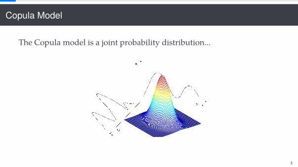
The Copula model is a joint probability distribution...
3

Motivating example

A Motivating Example
5

A Motivating Example
SELL!
6

A Motivating Example
7

8

UGM and Gaussian graphical

UGM and Multivariate Gaussian
Graph with nodes V and edges E.
G � (V, E)
p(x) ∼d∏
j�1φj(xj)
∏(i,j)∈E
φij(xi, xj)
10

UGM and Multivariate Gaussian
p(x) ∼ exp(−12
(x − µ)T∑
−1(x − µ))
p(x) ∼( d∏
i�1
d∏j�1
exp(−12
xixjΣ−1ij )︸ ︷︷ ︸
φij(xi ,xj)
) ( d∏i�1
exp(xivi)︸ ︷︷ ︸φi(xi)
)
# Pair-wise Markov property holds iff Σ−1v1,v2 � 0# Edges of G correspond with off-diagnol non-zero elements
11

Limitations of M. Gaussian and Motivation for Copula
Advantages of Gaussian GraphicalModel:# Covariance matrix conjugate
with G-Wishart prior.# Relatively easy to sample.# Overall cheap and simple.
Disadvantages of GaussianGraphical Model:# Unimodal joint distribution# Marginals are Gaussian# Random variables must be
continuous
12

Limitations of M. Gaussian and Motivation for Copula
13

Limitations of M. Gaussian and Motivation for Copula
14

Limitations of M. Gaussian and Motivation for Copula
Disadvantages of GaussianGraphical Model:# Uni-modal joint distribution# Marginals are Gaussian# Random variables must be
continuous
Solved by Copula Model:# Multi-modal joint distribution# Marginals can be arbitrary
functions# Both discrete and continuous
variables
15

Copula model

The Copula Model
If we have d random variables and we want to satisfy the followingconditions:
# Marginals can be arbitrary functions# Both discrete and continuous variables
Then what is the natural way to combine the random variables into ajoint distribution?Answer: use their CDF’s
17

Mapping the CDF
In order to allow continuous and discrete variables to "communicate,"we consider a joint distribution as a function of marginal CDF’s.
F(F1(x1), F2(x2), ..., Fd(xd))
But working in CDF space is not nice.Idea: we map the marginals CDF’s back into a latent variable.
F(φ−1[F1(x1)], φ−1[F2(x2)], ..., φ−1[Fd(xd)])
18

Mapping the CDF
Figure : Mapping from observed to latent variable via CDF. Multimodalto unimodal.
19

Mapping the CDF
Figure : Mapping from observed to latent variable via CDF. Multimodalto unimodal.
20

Mapping the CDF
Figure : Mapping from observed to latent variable via CDF. Multimodalto unimodal.
21

Mapping the CDF
We’ve been talking about mappingthe marginal of x to a latent variablebut do we know the marginals?
Yes! Given a set of data, we canapproximate marginals.
22

Gaussian Copula
Notation:
# ϕ(x) - standard normal density (PDF)# Φ(x) - standard normal Cumulative Distribution Function (CDF)# Φ−1(x) - Inverse CDF# Latent random variable Z# CDF F1(x1) � Φ(z1)# PDF f1(x1) � 1
σ1ϕ(z1)
23

Gaussian Copula
For any multivariate distribution, with CDF F and marginal CDF’s Fi,copula C is such distribution on [0, 1]d s.t.
F(x1, x2 . . . , xd) � C(F1(x1), . . . , F1(xd))
� C(φ−1[F1(x1)], φ−1[F2(x2)], . . . , φ−1[Fd(xd)])� C(z1, z2, . . . , zd)� Φd(z1, z2, . . . , zd)
(1)
We picked φ and Φd to be Gaussian but they could be Student-t, Laplace,etc.
24

Gaussian Copula
CDFF(x) � C(F1(x1), F2(x2), . . . , Fd(xd))
f (x) � c(F1(x1), F2(x2), . . . , Fd(xd))d∏
i�ifi(xi)
where fi(xi) is the marginal PDF.Copula density c is defined by:
c(F1(x1), F2(x2), . . . , Fd(xd)) �∂dC
∂F1 . . . ∂Fd
25

Chain Rule
# 2-D case
f (x, y) �∂2C(Fx(x), Fy(y))
∂X∂Y
�∂X
(∂Y
(C(Fx(x), Fx(y))
))�∂X
(∂C∂Fy
dFy
dy
)�
∂2C∂Fx∂Fy
·dFxdX
dFy
dY� copula density × product of marginal pdf
26

Gaussian Copula
PDF can be written with a correlation matrix K:
f (x) �1
|K|12exp{−
12
z(K−1 − I)zT}
d∏i�1
1σiϕ(zi)
wherezi � Φ
−1 [Fi(xi)]
Density of copula:
c(x) �1
|K|12exp(−
12
z(K−1 − I)zT)
27

Special Case: Uniform Correlation Structure
K �
*....,
1 ρ . . . ρρ 1 . . . ρ...
.... . .
...ρ ρ . . . 1
+////-
, ρ ∈ (−1
d − 1, 1]
Solving for K−1 and |K|,
c(x) � k1(ρ, d) ∗ exp{k2(ρ, d)
((d − 1)ρ
d∑i�1
z2i − 2d∑
j�1
∑i<j
zizj
)}
28

Special Case: Serial Correlation Structure
K �
*....,
1 ρ . . . ρd−1
ρ 1 . . . ρd−2
......
. . ....
ρd−1 ρd−2 . . . 1
+////-
, ρ ∈ (−1
d − 1, 1]
Solving for K−1 and |K|,
c(x) � k3(ρ, d) ∗ exp{k4(ρ, d)
(2ρ
d∑i�1
z2i − ρ(z21 + z2d) − 2d−1∑i�1
zizi+1
)}29

Copula inference

Inference
Given n points of d dimensional data x1:n, we would like to find therelationship between pairs of random variables.
G � (V, E) ⇒ {K|Kij � 0 if (i, j) < E}
P(Zi⊥Zj |Z−i−j) � 1 −1T
T∑t�1
Iij(Gt)
31

Pre-requisites
Markov properties associated with UGM for Z translate into Markovproperties for X [proof omitted]:
P(Xi⊥Xj |X−i−j) � P(Zi⊥Zj |Z−i−j) � 1 −1T
T∑t�1
Iij(Gt)
Iij(G) �
1, if (i, j) ∈ E0, otherwise
32

Inference can be done independent of marginals
Given x(1:n), any set of marginal CDF’s will obey the following constarintA on z(1:n):
A(x(1:n)) �[liv < zi
v < uiv : 1 ≤ i ≤ n, 1 ≤ v ≤ d
]liv � max{zk
v : xkv < xi
v}, uiv � min{zk
v : xiv < xk
v}
If z(1:n) obey constraint A, no need for marginals.
33

Inference can be done independent of marginals
Idea: Only order of zi matterbecause choosing Fi is simplychoosing a way to"connect-the-dots" in marginalCDF’s of x.
34

Inference
# G be a graph defining a gaussian graphical model for the latentvariables Zv
# Joint posterior distribution of K, the latent data z(1:n) and the Graphis,
p(K, z1:n,G|C) ∝ p(z1:n|K,C) × p(K|G) × p(G)
C is the event that z(1:n) obeys constraint A(x(1:n))
# Joint distribution is not defined if K < PG. PG is the set of symmetric,positive, definite matrices "obeying" graph G
35

Inference Algorithm
Since joint distribution is not defined for K < PG, construct Gibbssampling algorithm for the marginal:
p(z(1:n) ,G|C) �∫
K∈PG
p(K, z(1:n) ,G|C)dK
36

Gibbs sampling Algorithm
We have a joint density,
f (x, y1, ..., yk)
and we are interested in the marginal density,
f (x) �∫ ∫
..∫
f (x, y1, ..., yk)dy1, dy2, ...dyk
Assume we can sample the k + 1-many univariate conditional densities:
f (X|y1..., yk)f (Y1 |x, y2..., yk)f (Y2 |x, y1, y3..., yk)...f (Yk |x, y1, y3..., yk−1)
37

Gibbs sampling Algorithm
Choose arbitrarily, k initial values: Y1 � y01,Y2 � y02,Y3 � y03....Yk � y0k
x1 by a draw from f (X|y01, ..., y0k)
y11 by a draw from f (Y1 |x1, y02, ..., y0k)
y12 by a draw from f (Y2 |x1, y01, y03..., y
0k)
...y1k by a draw from f (Yk |x1, y11, ..., y
1k−1)
This constitutes one Gibbs "pass" through k+1 conditional distributions,yielding samples: (x1, y11, y
12, ...y
1k), (x2, y21, y
22, ...y
2k)...
The average of the conditional densities f (X|y1, ..yk) will be a closeapproximation to f (X)
38

Inference Algorithm
We would like to solve for the marginal:
p(z(1:n) ,G|C) �∫
K∈PG
p(K, z(1:n) ,G|C)dK
# Initialize variables to G0, K0, z(1:n) where z(1:n) obeys C# Sample G using Metropolis-Hastings# Sample K using block Gibbs-sampling# Sample z(1:n) using Gibbs-sampling# Repeat for T iterations
39

Inference Algorithm: Metropolis-Hasting
1. Sample G from the conditionalp(G|z(1:n) ,C) � p(G|z(1:n)) ∝ p(z(1:n)
|G)p(G)2. Propose Gnew where Gnew
∈ nbd(G)*3. Generate u from U(0, 1)4. Move to Gnew if
u <p(Gnew
|z(1:n))p(G|Gnew)p(G|z(1:n))p(Gnew |G)
* nbd(G) are all the graphs G∗ s.t. G∗ differs from G by the addition orsubtraction of one edge.# p(Gnew
|G) is the proposal function and is chosen.
40

Inference Algorithm:
p(G|z(1:n)) �p(z(1:n)
|G)p(G)p(z(1:n))
# We need to solve for p(z(1:n)|G), the marginal likelihood
# Solving the numerator gives estimate for p(z(1:n) ,G|C)
41

Inference Algorithm: Exploit Conjugacy
# We need to solve for p(z(1:n)|G), the marginal likelihood
# Z is Gaussian with G-Wishart prior
p(K) �1
IG(δ,D)|K|δ−2/2 exp
(−12〈K,D〉
)where 〈K,D〉 � tr(KTD) is the trace inner product.
42

Inference Algorithm: Exploit Conjugacy
# The marginal is the ratio of normalizing constants
p(z(1:n)|G) � IG(δ + n,D + U)/IG(δ,D)
where U �∑n
i�1(zi)T(zi)# If G is decomposable, then this can be solved explicitly, else use
numerical integration# Laplace approximation, other methods
43

Inference Algorithm: Block-Gibbs
We sample K from the posterior:
p(K|G, z(1:n) ,C) � p(K|G, z(1:n))
Again exploit the conjugacy of Gaussians:
p(K|G, z(1:n)) � WG(δ + n,D +
n∑i�1
(zi)T(zi))
44
Inference Algorithm: Block-Gibbs
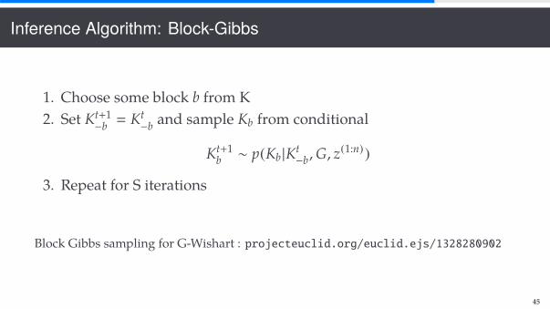
1. Choose some block b from K2. Set Kt+1
−b � Kt−b and sample Kb from conditional
Kt+1b ∼ p(Kb |Kt
−b,G, z(1:n))
3. Repeat for S iterations
Block Gibbs sampling for G-Wishart : projecteuclid.org/euclid.ejs/1328280902
45

Inference Algorithm: Gibbs
Having K, we sample z(1:n), noting independence between samples:
p(z(1:n)|K,G,C) �
n∏i�1
p(z(i)|K,C)
We sample z(i) independently and employ a Gibbs sampler withconditional:
p(z(i)v |z
(i)−v,K,C)
The conditional is truncated Gaussian. To impose C, we require
z(i)v ∈ [liv, ui
v]
46
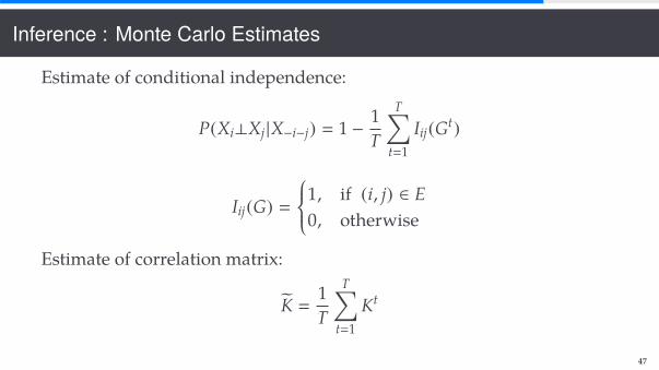
Inference : Monte Carlo Estimates
Estimate of conditional independence:
P(Xi⊥Xj |X−i−j) � 1 −1T
T∑t�1
Iij(Gt)
Iij(G) �
1, if (i, j) ∈ E0, otherwise
Estimate of correlation matrix:
K̃ �1T
T∑t�1
Kt
47

Inference : Monte Carlo Estimates
Estimate of correlation matrix:
K̃ �1T
T∑t�1
Kt
Estimate of Gaussian Copula CDF:
F(X) � C(F̂1(x1) . . . F̂p(xp) |K̃)
where F̂1(x1) is the empirical marginal distribution.
48

Sampling
Sampling x is easy once the correlation matrix is known.
# Sample Gaussian latent variable z# Map z back to x using empirical marginal distributions
uv � φ (̃zv)
x̃v � F̃−1v (uv)
49

Case Study

Case Study - Labor Force Survey Data
# Considers dependencies among income levels, educationalattainment, fertility and family background
# link: http://webapp.icpsr.umich.edu/GSSS/
51

Labor Force Survey Data
Variables TypeNEC - Income of the Respondent (INC) ordinal variable (21C)DEG - Highest degree obtained by therespondent ordinal variable (5C)
CHILD - number of children of therespondent count variable
PINC - financial status of the parents ofthe respondent ordinal variable (5c)
PDEG - highest degree obtained by therespondent’s parents an ordinal variable (5c)
PCHILD - number of children of therespondent’s parents count variable
AGE - respondent’s age in years count variable52

Results
Fig: Estimates of the posterior inclusion probability of edges (CHILD,PINC) and (DEG, PCHILD) across iterations.
0 2000 4000 6000
0.0
0.2
0.4
0.6
0.8
1.0
CHILD − PINC
Iteration
Edg
e P
roba
bilit
y
0 2000 4000 6000
0.0
0.2
0.4
0.6
0.8
1.0
DEG − PCHILD
IterationE
dge
Pro
babi
lity
Figure 4.1: Estimates of the posterior inclusion probability of edges (CHILD, PINC) and (DEG,PCHILD) across iterations.
Hoff (9) assessed links between variables in this dataset by inspecting the 95% credible inter-vals for the regression coefficients to see if they have spanned zero. The main conclusions resultingfrom our copula Gaussian graphical models approach are shared by Hoff (9) though we differ intwo instances. First, our method shows a high probability (essentially one) of an edge betweenCHILD and PCHILD, while this link was absent in Hoff (9). Such an inclusion seems sensible,as individual fertility levels are likely to be related to historical fertility in a given family. Further-more, we place only a 20% inclusion probability on an edge between PINC and PCHILD, thoughthis connection was displayed in Hoff (9).
Table 4.1: Posterior estimates of the off-diagonal elements of Υ and posterior inclusion probabilityof edges for the labor force data.
Variable 1 Variable 2 Entry in Υ Edge ProbabilityCHILD INC 0.292 0.997CHILD PCHILD 0.22 0.999CHILD PDEG -0.262 0.953CHILD AGE 0.599 1INC DEG 0.489 1INC AGE 0.34 1DEG PCHILD -0.187 0.668DEG PDEG 0.473 1PCHILD PDEG -0.303 0.991PINC PDEG 0.453 1PDEG AGE -0.232 0.988
9
53

Results
Table: Posterior estimates of the off-diagonal elements of and posteriorinclusion probability of edges for the labor force data
0 2000 4000 6000
0.0
0.2
0.4
0.6
0.8
1.0
CHILD − PINC
Iteration
Edg
e P
roba
bilit
y
0 2000 4000 6000
0.0
0.2
0.4
0.6
0.8
1.0
DEG − PCHILD
Iteration
Edg
e P
roba
bilit
y
Figure 4.1: Estimates of the posterior inclusion probability of edges (CHILD, PINC) and (DEG,PCHILD) across iterations.
Hoff (9) assessed links between variables in this dataset by inspecting the 95% credible inter-vals for the regression coefficients to see if they have spanned zero. The main conclusions resultingfrom our copula Gaussian graphical models approach are shared by Hoff (9) though we differ intwo instances. First, our method shows a high probability (essentially one) of an edge betweenCHILD and PCHILD, while this link was absent in Hoff (9). Such an inclusion seems sensible,as individual fertility levels are likely to be related to historical fertility in a given family. Further-more, we place only a 20% inclusion probability on an edge between PINC and PCHILD, thoughthis connection was displayed in Hoff (9).
Table 4.1: Posterior estimates of the off-diagonal elements of Υ and posterior inclusion probabilityof edges for the labor force data.
Variable 1 Variable 2 Entry in Υ Edge ProbabilityCHILD INC 0.292 0.997CHILD PCHILD 0.22 0.999CHILD PDEG -0.262 0.953CHILD AGE 0.599 1INC DEG 0.489 1INC AGE 0.34 1DEG PCHILD -0.187 0.668DEG PDEG 0.473 1PCHILD PDEG -0.303 0.991PINC PDEG 0.453 1PDEG AGE -0.232 0.988
9 54

Closing remarks

Summary
We’ve covered an introduction to Copula Models:
# Advantages of Copula models over traditional Gaussian# The Gaussian Copula model# Inference using Copula model
56

Further Readings
# Copula Gaussian Graphical Models (https://www.stat.washington.edu/research/reports/2009/tr555.pdf)
Recent paper and accompanying code:
# Variational Gaussian Copula Inferencepeople.ee.duke.edu/~lcarin/VGC_AISTATS2016.pdf
# github.com/shaobohan/VariationalGaussianCopula
Copula models in a financial setting:
# Modelling the dependence structure of financial assets: A survey offour copulas www.nr.no/files/samba/bff/SAMBA2204.pdf
57


