
FIVVBOWWCMNSIC 1
Fusing Integrated Visual Vocabularies-Based Bag of Visual Words
and Weighted Colour Moments on Spatial Pyramid Layout for
Natural Scene Image Classification
Yousef Alqasrawi, Daniel Neagu, Peter Cowling
School of Computing, Informatics and Media (SCIM), University of Bradford, Bradford, BD7 1DP, UK
Abstract
The bag of visual words (BOW) model is an efficient image representation technique for
image categorisation and annotation tasks. Building good visual vocabularies, from
automatically extracted image feature vectors, produces discriminative visual words which
can improve the accuracy of image categorisation tasks. Most approaches that use the BOW
model in categorising images ignore useful information that can be obtained from image
classes to build visual vocabularies. Moreover, most BOW models use intensity features
extracted from local regions and disregard colour information which is an important
characteristic of any natural scene image. In this paper we show that integrating visual
vocabularies generated from each image category, improves the BOW image representation
and improves accuracy in natural scene image classification. We use a keypoints density-
based weighting method, to combine the BOW representation with image colour information
on a spatial pyramid layout. In addition, we show that visual vocabularies generated from
training images of one scene image dataset, can plausibly represent another scene image
dataset on the same domain. This helps in reducing time and effort needed to build new
visual vocabularies. The proposed approach is evaluated over three well-known scene
classification datasets with 6, 8 and 15 scene categories respectively using 10-fold cross-
validation. The experimental results, using support vector machines with histogram
intersection kernel, show that the proposed approach outperforms baseline methods such as
Gist features, rgbSIFT features and different configurations of the BOW model.
Keywords: image classification, natural scenes, bag of visual words, integrated visual
vocabulary, pyramidal colour moments, feature fusion, semantic modelling.
FIVVBOWWCMNSIC 2
1. Introduction
The availability of low-cost image capturing devices and the popularity of photo-sharing
websites such as Flickr and Facebook have led to a dramatic increase in the size of image
collections. For efficient use of such large image collections, image categorisation, searching,
browsing and retrieval techniques are required [1-3].
Scene classification has been investigated in two complementary research areas,
understanding human visual perception of scenes and developing computer vision techniques
for automatic scene categorisation. This entail reveals how humans are able to understand,
analyse and represent scenes, which is of great research interest in many psychological
studies. Knowledge from these studies can help computer vision researchers design and
develop systems to close the gap between human semantic and image low-level information
[4, 5]. From the computer vision viewpoint, scene classification is the task of automatically
assigning an unlabelled image into one of several predefined classes (e.g., beach, coast or
forest). It provides contextual information to help other processes such as object recognition,
content-based image retrieval and image understanding [6, 44]. However, designing and
implementing algorithms that are capable of successfully recognising image categories
remains a challenging problem [7]. This is because of illumination changes, scale variations,
occlusions, large variations between images belonging to the same class and small variations
between images in different classes.
In recent years, local invariant features or local semantic concepts [14] and the bag of
visual words (BOW) became very popular in computer vision and have shown impressive
levels of performance in scene image classification [6, 12, 15-19]. There are two main parts
to build an image classification system within the BOW framework. The first relates to the
extraction of features that characterise image content. The work described in this paper
relates to this part. The second part is the classifier. The elements needed to build a bag of
visual words are: feature detection, feature description, visual vocabulary construction and
image representation, each step is performed independently of the others.
Recently, a range of new methods have been advanced to improve the performance of the
conventional BOW paradigm. We can classify these methods into three main categories. The
first category attempts to improve the construction of the visual vocabulary [20-24]. The
second category suggests using multiple features with weighting techniques to combine
features [18, 25-28]. In the third category, techniques that add spatial information over the
BOW have been proven to improve the performance of scene classification tasks [29-32].
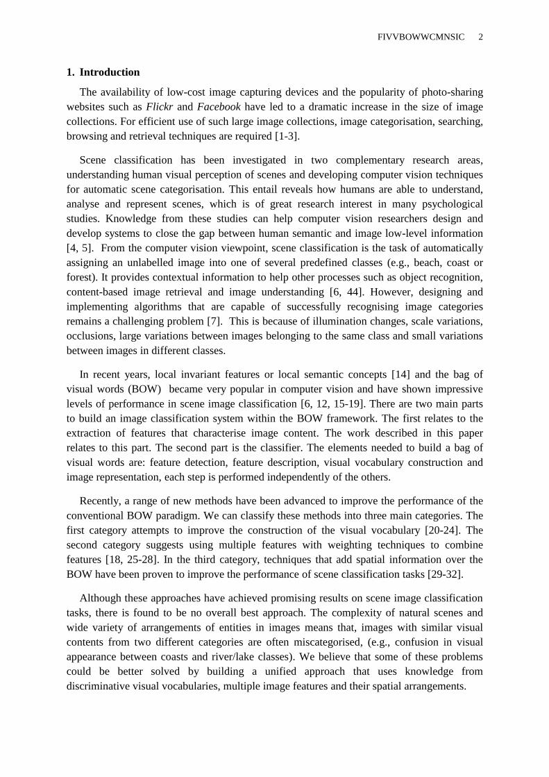
Although these approaches have achieved promising results on scene image classification
tasks, there is found to be no overall best approach. The complexity of natural scenes and
wide variety of arrangements of entities in images means that, images with similar visual
contents from two different categories are often miscategorised, (e.g., confusion in visual
appearance between coasts and river/lake classes). We believe that some of these problems
could be better solved by building a unified approach that uses knowledge from
discriminative visual vocabularies, multiple image features and their spatial arrangements.

FIVVBOWWCMNSIC 3
In this paper, we build upon the work of Alqasrawi et al. [26] to improve categorisation
performance for natural scene images. In our previous work [26], we introduced a weighting
approach to fuse image colour information, with the traditional bag of visual word model for
natural scene image classification. In this paper, we focus on learning discriminative visual
words from image classes separately, in order to map local keypoints to most representative
visual words.
In this work, we propose integrating knowledge from discriminative visual vocabularies
learned from image classes, multiple image features and spatial arrangements information to
improve the conventional bag of visual words, for natural scene image classification task. To
improve visual vocabulary construction, visual vocabularies extracted from the training
images of each scene image category are combined into a single integrated visual
vocabulary. It is composed of discriminative visual words from different scene categories.
The proposed approach is extensively evaluated over three well-known scene classification
datasets with 6, 8 and 15 scene categories [7, 11, 29] respectively using 10-fold cross
validation. We tested our work on a fourth dataset with 4 scene classes. This dataset is a
subset of 8 scene classes [11] composing natural scene images with no man-made objects
(refer to section 5.2). We will show in this paper that the integrated visual vocabulary is more
discriminative than the universal visual vocabulary to build BOW histograms. Moreover, we
show that the Keypoint Density-based Weighting (KDW) method proposed in [26] can be
used effectively with the integrated visual vocabulary, to control the fusion of image colour
information and BOW histograms on a spatial pyramid layout. We compare our approach to a
number of baseline methods such as Gist features [11], rgbSIFT features [47] and different
configurations of conventional BOW.
The rest of this paper is organised as follows. In section 2, we give an overview of related
work. In section 3, we describe the three main steps needed to represent and summarise
image contents. We describe our approach for merging colour information with BOW in
section 4. We present our experimental setup and results in section 5 and we conclude the
paper in section 6.
2. Related work
Early work in scene image classification (low-level processing) was based on low-level
image features such as colour and texture, extracted automatically from the whole image or
from image regions [2, 8-11]. Methods based on global image features often failed to
successfully represent the high-level semantics of user perception [2, 3]. Semantic modelling
(mid-level processing) uses an intermediate semantic level representation, falling between
low-level image features and (high-level) image classification, in an attempt to narrow the
semantic gap between low-level features and high-level semantic concepts [7, 12]. A simple
way to represent a semantic concept is to partition an image into blocks and then label each
block manually with one or more semantic concepts [7, 13]. However, such systems are
found to be time consuming and expensive. A recent survey on state of the art techniques for
scene classification that exploits features on the spatial domain, frequency domain and
constrained domain is presented in [45].

FIVVBOWWCMNSIC 4
Researchers in computer vision have recently started to make use of techniques based on
text document retrieval, to represent image contents in image classification and retrieval
systems [34]. The bag of words approach is one of these techniques and is very common in
text-based information retrieval systems. The analogy between document and image is that
both contain information. However, the main obstacle is how to extract semantic “visual
words” from image content. In the literature, much work has been done in image/object
classification and retrieval based on the bag of visual words approach. We review those
approaches most strongly connected with the work of this paper below.
Zhu et al. [34] are perhaps the firsts who tried to represent images using an analogue of the
bag of words approach. In their work, images are partitioned into equal size blocks which are
then indexed using a visual vocabulary, whose entries are obtained from the block features.
The bag of visual words approach received a substantial increase in popularity and
effectiveness with the development of robust salient features detectors and descriptors such as
Scale Invariant Feature Transform (SIFT) [17]. Csurka et al. [19] and Sivic et al. [35] showed
how to use the bag of visual words by clustering the low-level features using the K-means
algorithm, where each cluster corresponds to a visual word. To build the bag of visual words,
each feature vector is assigned to its closest cluster. Perronnin et al. [23] proposed the use of
adapted vocabularies by combining universal vocabularies with class-specific vocabularies.
In their work, a universal visual vocabulary is learned to describe the visual features of all
considered image classes. Then, class-specific vocabularies are combined with the universal
vocabulary to refine accuracy. Perronnin et al‟s work is an interesting contribution to the
computation of distinctive visual vocabularies. However, their proposed adapted vocabulary
does not show the differences between scene classes and it handles only one kind of image
feature. Another contribution to build discriminative visual vocabularies has been
investigated by Jurie and Triggs [36], which proposes a clustering algorithm to build a visual
vocabulary. Their algorithm produces an ordered list of centers. A quantisation rule is used
in such a way that patches are assigned to the first center in the list that lies within a fixed
radius r, and left unlabelled if there is no such center. In Nilsback and Zisserman [37], three
different visual vocabularies are created to represent colour, shape and texture properties of
flower images. These visual vocabularies are combined to obtain a weighted joint frequency
histogram. In Nister and Stewenius [22], local features extracted from images are
hierarchically quantised in a vocabulary tree. It was shown that retrieval results are improved
with a larger vocabulary.
Four different approaches are investigated in [38] to create compacted visual vocabulary,
while retaining classification performance. The four approaches consists of 1) global visual
vocabulary construction; 2) class-specific visual vocabulary construction; 3) annotating a
semantic vocabulary and 4) soft-assignment of image features to visual words. These
approaches were evaluated against each other on a large dataset. The experimental results
suggested that best method depends uppon application at hand. Also, in a different context,
an approach to integrate different vocabularies has been introduced in [46] to build bag of
phrases for near duplicate image detection.
FIVVBOWWCMNSIC 5
A bag of visual words represents an image as an orderless collection of local features,
without spatial information. Spatial pyramid matching was proposed by Lazebnik and
Raginsky [14] as an extension to the orderless bag of visual words. The spatial pyramid
divides the image into 1x1, 2x2, 4x4, etc. regions. Assuming a visual vocabulary is given;
local features extracted from each region are quantised and then combined using a weighting
scheme which depends on region level. Based on this approach, three different hierarchical
subdivisions of image regions were recently proposed for recognising scene categories [32].
Most work that used BOW and spatial pyramid matching focuses mainly on intensity
information analysis and discards image colour information. We believe colour information
has an equally significant importance in recognising natural scene image categories. Many
studies have investigated including multiple image features within the framework of BOW
[18, 26, 28]. Early fusion and late fusion are the two main approaches used to combine
different types of image features. In the early fusion approach, features were combined before
building visual vocabularies. In late fusion, each feature has its own visual vocabulary. The
fusion of colour and intensity information on the BOW paradigm is proposed by Quelhas et
al. [18]. Quantised colour information and the BOW are computed over local interest
regions. Although this approach has shown an improvement in classification accuracy, it has
two main limitations: (1) Colour information is computed over interest regions only; and (2)
No spatial information is implemented. In [28] a novel approach is proposed to recognise
object categories using multiple image features. Their model, the Top-Down Colour
Attention model, considers two properties for image representation: feature binding and
vocabulary compactness. The first property involves combining colour and shape features at
the local level, while the second property concerns separate visual vocabularies for each of
the two features. Very recently, a number of visual patch weighting methods and different
configurations of BOW fused with multiple image features have been investigated by Jiang et
al. [39] for semantic concept detection in video images. The invariance properties and the
distinctiveness of colour descriptors, such as rgbSIFT features, are studied recently by Sande
at el. [47] for object and scene classification tasks. They proposed a systematic approach to
provide a set of invariance properties, such as invariance to light intensity.
3. Location-Aware Image Semantic Representation
In this section we introduce the main steps needed to construct four forms of bag of visual
words which will be used in this work to represent visual image content:
Universal BOW (UBOW) based on universal visual vocabulary.
Integrated BOW (IBOW) based on class-specific visual vocabularies.
Universal Pyramid BOW (UPBOW) similar to UBOW but on spatial pyramid layout.
Integrated Pyramid BOW (IPBOW) similar to IBOW but on spatial pyramid layout.
The following subsections details all steps required to build these four BOW image
representations. In each case we will consider how we extract and describe local features
FIVVBOWWCMNSIC 6
from images, build universal and integrated visual vocabularies and map local features to the
closest visual words on spatial pyramid layout.
3.1. Local invariant points detection and description
In this work we use the Difference of Gaussian (DoG) point detectors and SIFT
descriptors [17] to detect and describe local interest points or patches from images.
Generally, these methods show good performance compared to other methods in the literature
[40]. The DoG detector has properties of invariance to translation, rotation, scale and constant
illumination changes. Once local invariant points are defined, SIFT descriptors are used to
capture the structure of the local image patches and are defined as local histograms of edge
directions computed over different parts of the patch. Each patch is partitioned into 4x4 parts
and each part is represented by a histogram of 8 orientations (bins) that gives a feature vector
of size 128. In this paper we use the binaries provided at [41] to detect DoG local points and
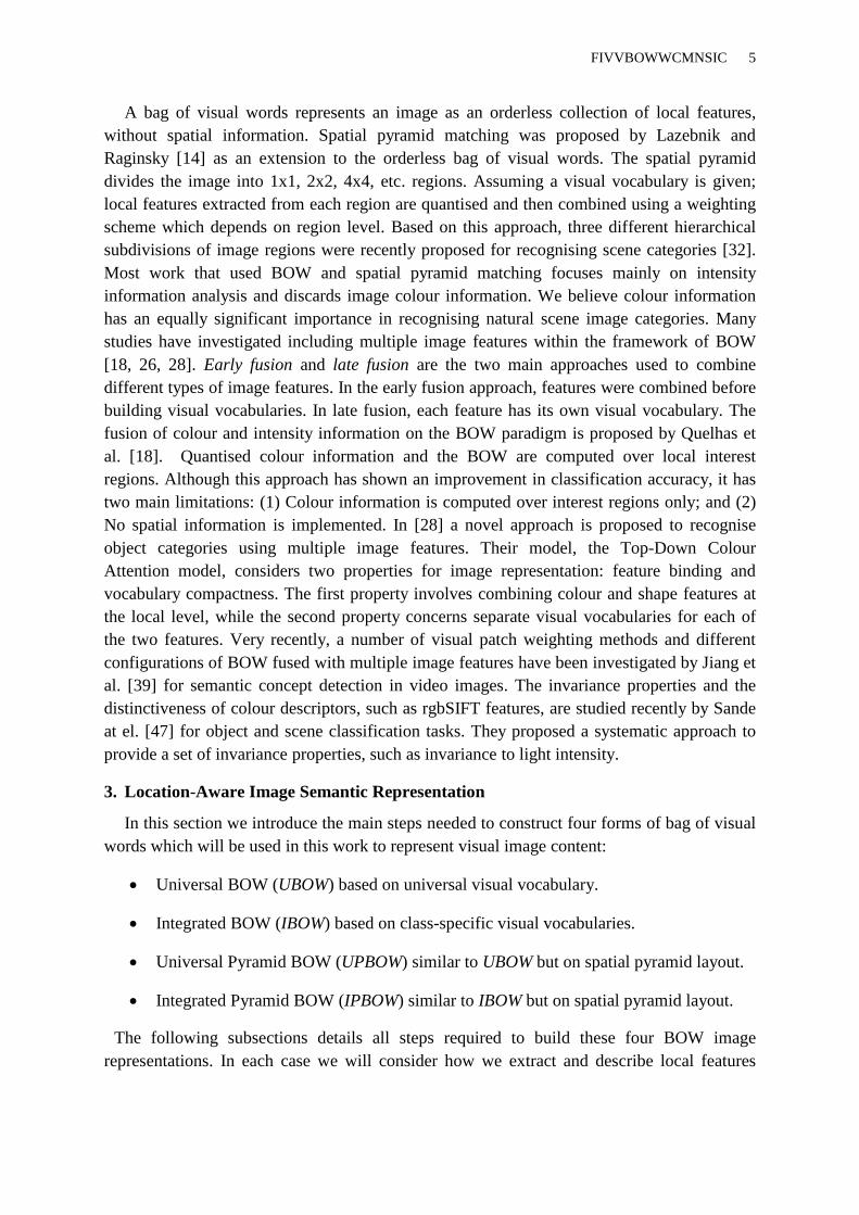
to compute the 128-D real valued SIFT descriptors from them. This process is described in
Fig 1. Features extracted from all images are stored in Features Database. In section 3.2 we
describe how this is used to build visual vocabularies.
3.2. Visual Vocabulary Construction
In this section, we describe how to learn both the universal visual vocabulary and the
proposed integrated visual vocabulary that will be used in the rest of this paper. To obtain the
visual vocabulary, we use feature vectors (SIFT features) stored in image Features Database
as described in section 3.1. All feature vectors from all training images on the dataset are
Image Database
Fea
ture
det
ecti
on
Fea
ture
des
crip
tio
n
Features Database
Fig. 1 Keypoint detection and description process. The circles overlaid on the image indicate
keypoints located using DoG feature detector. Each keypoint is described and stored in feature
vector. Each feature vector contains 128 descriptive values, using SIFT descriptors.

FIVVBOWWCMNSIC 7
quantized, using the k-means algorithm, to obtain k centroids or clusters. These centroids
represent visual words. The k visual words constitute the universal visual vocabulary. This
vocabulary is used to build the UBOW and the UPBOW. For the integrated visual
vocabulary, SIFT features from all training images of each scene class are clustered into k
visual words. More formally: Let MCCCC ,..,, 21 be the set of M scene classes
considered. Let MVVVV ,..,, 21 be the set of M class-specific vocabularies. Each
jkjjj VVVV ,..,, 21 is a set of k visual words learned from all training images of class j .
We call V the integrated visual vocabulary. This vocabulary is used later to build IBOW and
IPBOW.
The rationale behind building an integrated visual vocabulary is to try to find more
specific discriminative visual words from each image class in order to avoid interference with
other classes. In the universal visual vocabulary, visual words that belong to a specific
concept (e.g., foliage) may be assigned to a cluster or visual word of a different concept (e.g.,
rock). We believe that our integrated visual vocabulary may be robust enough to incorporate
naturally existing intra-class variations to discriminate between different image classes. For
example, building visual vocabulary for coasts scene images would contain informative
information about water, sand and sky, in contrast to other scene classes such as mountains.
Fig. 2 shows details of how to construct both kinds of visual vocabularies. We will show later
in the experimental results section how the distribution of the mean of all IBOW of training
images are different and more informative and discriminative than the UBOW generated
from universal visual vocabulary (see Fig. 10 for differences between universal and
integrated visual vocabularies).
3.3. Summarising image content using the BOW
The Bag of Visual Words provides a summary of image contents. In section 3.1, we
discussed feature detection and description of image content. Section 3.2 showed how to
build universal and integrated visual vocabularies from image local features. For simplicity,
we refer to both IBOW and UBOW more generally as BOW (which differ in which kind of
Features Database
Qu
anti
zati
on
(K
-mea
ns)
Un
iver
sal
Vis
ual
Vo
cabula
ry
Class 1
Features
Class 2
Features
Class M
Features
Qu
anti
zati
on
(K
-mea
ns)
Class 1
Visual Voc.
Class 2
Visual Voc.
Class M
Visual Voc.
Inte
gra
ted
Vis
ual
Vo
cabu
lary
Fig. 2 Visual vocabulary construction process. The left side of Features database shows universal visual
vocabulary. The right side shows the proposed integrated visual vocabulary. Each class features (for class
1,2,…, M) represents feature vectors of training images for a specific image category.

FIVVBOWWCMNSIC 8
vocabulary we use to build them). To build the BOW histogram, each image SIFT descriptor
is assigned to the index of the nearest cluster in the visual vocabulary. The visual words in the
context of this paper refer to the cluster centres (centroids) produced by the k-means
clustering algorithm. Let V denote the set of all visual words produced from the clustering
step over a set of local point descriptors VivV i ,..,1 , where iv is the i -th visual word
(or cluster) and V is the size of the visual vocabulary. We use a vocabulary of size 200 for
both the universal visual vocabulary and for class specific visual vocabulary. In the case of
the integrated visual vocabulary, V
is 200M (where M is the number of classes).
Experiments showed no improvements in performance beyond 200 [29]. The set of all SIFT
descriptors for each image d is mapped into a histogram of visual words dh at image-
level, such that:
Vifdhd
j
N
j
i
di ,..,1,)(1
)(
(1)
otherwise
liVlvuvuf ljiji
d j,0
and ,..,1,,1)( (2)
where:
)(dhi is the number of descriptors in image d having the closest distance to the i -th visual
word iv and dN is the total number of descriptors in image d . )(i
d jf is equal to one if the j -
th descriptor ju in image d is closest to visual word iv among other visual words in the
vocabulary V .
3.4.Spatial pyramid Layout
Although the orderless bag of visual words approach is widely used and has made a
noticeable increase of performance in object/scene image modelling, it seems likely that we
can enhance it for scene recognition tasks by incorporating spatial information. Spatial
pyramid matching [29] works by repeatedly subdividing an image into increasingly finer sub-
regions and then computing histograms of local patches found inside each image sub-region.
An image is represented as a concatenation of weighted histograms at all levels of divisions.
In this paper, spatial pyramid layout refers to representing images by placing a sequence of
increasingly coarser grids over an image. Here we did not penalise local histograms of BOW
as described in [29, 32], since the experiments showed that to do so decreases the
classification accuracy of our system.
4. Pyramidal fusing of BOW and image colour information
In this section, we show how to model image semantic information based on merging
BOW and colour moments using a spatial pyramid layout. The motivation of our approach is
that most techniques that use BOW rely only on intensity information extracted from local
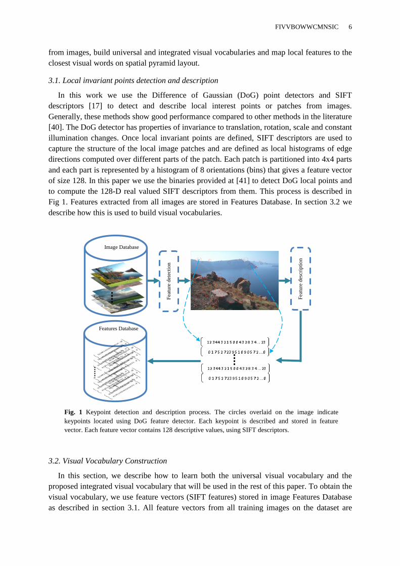
FIVVBOWWCMNSIC 9
invariant points and neglect colour information which seems likely to help in recognition
performance for scene image categories. We can see in Fig.3 an image with circles around a
rather dense set of interest points produced by DoG detectors. We see that interest points are
not uniformly distributed across the image, but rather are clustered on salient regions in the
scene. In natural scene images, colour information has a significant effect in discriminating
image areas such as sky, water and sand. Hence, we believe that merging colour information
and the BOW will be significant in modelling image visual semantics.
(a) (b)
Fig. 3 (a) Sample image with circles around interest points. (b) Sky and water contain little information of
interest. Red borders in (b) shows important information that helps discriminate image content.
Pyramid BOW Pyramid colour moments
image (d)
)(ir
l dc )(ir
l dh
Spatial pyramid layout fusing approach to
produce the feature vector )(dH
l = 0
1r
l = 1
1r 3r
2r 4r
l = 2
1r 5r 9r 13r
2r 6r 10r 14r
3r 7r 11r 15r
4r 8r 12r 16r
l = 1
1r 3r
2r 4r
l = 0
1r
l = 2 1r 5r 9r 13r
2r 6r 10r 14r
3r 7r 11r 15r
4r 8r 12r 16r
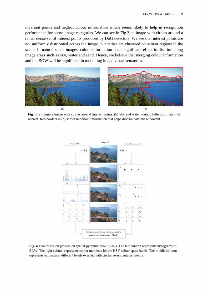
Fig. 4 Feature fusion process on spatial pyramid layout (L=2). The left column represents histograms of
BOW. The right column represents colour moments for the HSV colour space bands. The middle column
represents an image at different levels overlaid with circles around interest points.

FIVVBOWWCMNSIC 10
In our previous work [26], we proposed the Keypoint Density-based Weighting method
(KDW) for merging colour information and BOW over image sub-regions at all granularities
on the spatial pyramid layout. The KDW method aims to regulate how important colour
information is in each image sub-region before fusing it with BOW. The spatial pyramid
layout (refer to Fig. 4) works by splitting an image into increasingly coarser grids to encode
spatial locations of image local points. Hence an image with 2L levels, will have three
different representations with 21))2((0
2
L
l
l image sub-regions overall. Each image sub-
region is represented by a combination of the BOW and a weighted colour moments vector of
size 6 on the HSV colour space (2 for Hue, 2 for Saturation and 2 for Value). Both colour
moments and the BOW histogram are normalised to be unit vectors before the merging
process. An image with number of levels 2L and a visual vocabulary of size 200 will
produce a vector of dimension 4326.
We formulate our proposed approach below:
Let L denotes the number of levels, Ll ,...,1,0 , needed to represent an image d on the
spatial pyramid layout, i.e., an image d will have a sequence of L grids of increasingly finer
granularity. Let )(ir
l dh and )(ir
l dc denote a histogram vector of BOW computed using
equation (1) and the colour moments vector respectively. Both are computed from an image
d at level l and sub-region ir , 2)2(,..,1 li .
The concept of Keypoint Density-based Weight (KDW): Colour moment vector )(ir
l dc is
assigned a high weight on image sub-regions that have a keypoint density below thresholdl
riT .
Colour information will be less important in image sub-regions with high number of local
interest points. The threshold T is a real valued vector. Each component represents the
average density of keypoints (number of keypoints) at specific image sub-region over all
training images. We proposed the keypoint density-based weight as:
m
j
j
r
ll
r iidh
mT
1
)(1
(3)
where m is the number of images in the training image dataset. The components of the
threshold vector, which is the average keypoint density of all images at specific sub-regions
and granularity, help in making a decision about the importance of colour information at
specific image sub-region. The unified feature vector )(dH for image d is a concatenation of
weighted colour moments and BOW at all levels and over all granularities:
))(),(),...,(),((
)),(),(),...,(),(()),(),(()(
2)2(2)2(2)2(111
444111111
111111000
LLL r
LL
rr
L
r
LL
rr
L
rrrrrrrrr
dcwdhdcwdh
dcwdhdcwdhdcwdhdH
(4)

FIVVBOWWCMNSIC 11
otherwise
Tdhw
V
j
l
rr
l
jl
rii
i
,5.0
)(,11
(5)
We should notice that the values of weights w are non-negative numbers to indicate the
importance of colour information. We aim to cause images from the same category to be
close, and images from different categories to be far away in the new image representation.
Values for the weights have been obtained empirically during learning the support vector
machine SVM classifiers [43]. We should notice that weight values are highly dependent on
the threshold vector obtained from equation (3). Here, we use the proposed integrated visual
vocabulary described in section 3.2 and the spatial pyramid layout to generate IBOW and
IPBOW histograms. Fusing weighted pyramidal colour moments (WPCM) with the IBOW
and IPBOW histograms using equation (4) we obtain improved image representation
(IBOW+W_PCM and IPBOW+W_PCM). We assume that building visual vocabularies from
individual scene classes could produce more discriminative visual words than using universal
vocabulary. To justify this assumption, all UBOW and IBOW histograms generated from
training images of Vogel‟s dataset [7], described in section 5.2, have been averaged to see the
distribution of both BOWs in each scene class. Fig. 10 shows the difference between both
averages. Some sample BOW histograms are shown and they tend to be similar or close to
their average vector.
5. Experimental setup
The first part of this section presents the support vector machine (SVM) classifier and the
protocol we follow in all our experiments. Next, we describe the origin and composition of
datasets we use in our experiments. Experimental results are then reported with discussion.
We use the confusion matrix to assess the performance of all considered experiments.
5.1. Scene classifier
Multi-class classification is done using a support vector machine (SVM) with a histogram
intersection kernel. We use SVM in our study as they have been empirically shown to yield
higher classification accuracy in scene and text classification tasks [18, 26, 28]. Variations in
the classification accuracy are possible due to our choice of SVM kernel function. In this
work, we use the histogram intersection kernel. Many studies in image classification observe
that the histogram intersection SVM kernel is very useful. Moreover, histogram intersection
has been shown more effective than the Euclidean distance in supervised learning tasks [24,
29]. Odone et al. [42] proved that histogram intersection is a Mercer kernel and thus can be
used as a similarity measure in kernel based methods. Given two BOW histograms 1dh and
2dh , the histogram intersection kernel is:
i
iidhdhdhdhK ))(),(min())(),(( 2121 (6)
The protocol we follow for each of the classification experiments was as follows: All
experiments have been validated, using 10-fold cross validation where 90% of all images are

FIVVBOWWCMNSIC 12
selected randomly for learning the SVM and the remaining 10% are used for testing. The
procedure is repeated 10 times such that all images are actually tested by the SVM classifier.
The average of the results over the 10 splits yields the overall classification accuracy. To
implement the SVM method we used the publicly available LIBSVM software [43],
dedicated to Matlab, where all parameters are selected based on 10-fold cross validation on
each training fold. We use one-against-one multi-classification approach that results in
2
)1( MM two-class SVMs for M scene classes.
5.2.Image datasets
There are many image datasets available in the computer vision literature, but most of
them are dedicated to object detection and categorisation tasks. Performance of the proposed
scene classification approach is tested on two types of image datasets: a dataset with natural
scene images only, which is our main concern, and datasets with heterogeneous images
including different kind of images. The reason for choosing natural scene images is that they
generally are difficult to categorise in contrast to object-level classification because natural
scenes constitute a very heterogeneous and complex stimulus class [4]. Also, we considered
scene images that constitute artificial objects to allow fair and straightforward comparison
with state-of-the-art scene classification methods. Four datasets were used in our
experiments:
Dataset 1: This dataset, kindly provided by Vogel et al. [7], contains natural scene images
only with no man-made objects. It contains a total of 700 colour images of resolution 720
280 and distributed over 6 categories. The categories and number of images used are: coasts,
142; rivers/lakes, 111; forests, 103; plains, 131; mountains, 179; sky/clouds, 34. One
challenge in this image dataset is the ambiguity and diversity of inter-class similarities and
intra-class differences which makes the classification task more challenging.
Dataset 2: This dataset is a subset of the Oliva and Torralba [11] dataset. It constitutes
images of natural scene categories with no artificial objects, which are semantically similar to
images in Dataset1 and is distributed as follows: coasts, 360; forest, 328; mountain, 374;
open country, 410. The total number of images in this dataset is 1472.
Dataset 3: This dataset contains heterogeneous image categories. It consists of a total of
2688 colour images, 256x256 pixels, and distributed over 8 outdoor categories. The
categories and number of images used are: coast, 360; forest, 328; mountain, 374; open
country, 410; highway, 260; inside city, 308; tall building, 356; street, 292. This dataset is
created by Oliva and Torralba [11] and is available online at http://cvcl.mit.edu/database.htm.
Dataset 4: This dataset, provided by Lazebnik et al. [29], contains 15 heterogeneous
natural scene image categories. All images in this dataset are grayscale images (i.e., no colour
images). It contains different kind of images and the average image size is 300x250 pixels.
Images are distributed over categories as follow: highway, 260; inside city, 308; tall building,
356; street, 292; suburb, 241; forest, 328; coast, 360; mountain, 374; open country, 410;
bedroom, 216; kitchen, 210; living room, 289; office, 215; industrial, 311; store, 315. The

FIVVBOWWCMNSIC 13
first 8 categories were from Oliva and Torralba [11] and the first 13 were from Li and Perona
[12]. Fig. 5 depicts sample images from the four datasets aforementioned with different
image classes.
5.3.Feature extraction
In this work, we used Matlab to conduct all experiments. As we mentioned earlier, in the
experiments we perform 10-fold cross validation in order to achieve more accurate
performance estimation. The binaries provided by [40] are used to detect and describe local
Plain Mountain Sky/cloud
Coast River/lake Forest
(a) Dataset 1
Fig. 5 Some examples of the images used for each category from the Dataset 1, Dataset 2, Dataset3 and
Dataset 4 respectively.
(b) Dataset 3
Open country Mountain Forest Coast
Street Tall building Inside city Highway
(c) Dataset 2
(d) Dataset 4
Coast Forest Mountain Open country Suburb Highway Store Industrial
Inside city Tall building Street Kitchen Bedroom Office Living room
FIVVBOWWCMNSIC 14
keypoints using DoG and SIFT as parameters. Further we extracted basic rgbSIFT features
with local keypoint detection and standard parameters using the Color Descriptor software
provided by [47]. To build different visual BOW histograms, SIFT and rgbSIFT features
extracted from training images are used to build 10 visual vocabularies, one for each fold.
Gist features are extracted from images using the implementation provided by Oliva and
Torralba at (http://people.csail.mit.edu/torralba/code/spatialenvelope/).
5.4. Experimental results
In this section, we conduct extensive experiments to empirically evaluate the performance
of our proposed approach and compare it to the existing baseline and BOW models for
natural scene image categorisation tasks. We present four sets of experiments each
corresponds to one of the datasets mentioned in section 5.2. In the first experiments, we
tested the performance of our proposed approach on colour natural scene images with no
artificial objects, i.e., Dataset 1 and Dataset 2 respectively. The performance of our proposed
approach is compared with Gist features, improved Gist features and different configurations
of BOW models generated from SIFT features and rgbSIFT features. All visual vocabularies
employed in our experiments are generated separately for SIFT and rgbSIFT features. In the
second experiments, we test our proposed approach on Dataset 3 which contains different
kind of images and scene categories. We intend to find out how our approach performs on
heterogeneous set of scene classes. In the third experiment, we use grayscale images, Dataset
4, to test the performance of our proposed approach on large number of images and scene
categories. In the last experiment, we investigate the possibility of using visual vocabularies
generated from Dataset 1 to produce IBOW for Dataset 2.
Firstly, we present the classification performance of Gist features and improved Gist
features (i.e., Gist with pyramidal colour moments) tested on Dataset 1 and 2. The Gist
descriptor [11] uses a low dimensional representation of the scene which does not require any
segmentation process. A bank of Gabor filters are employed in the frequency domain and
tuned to different orientations and scales. The image is divided into a 44 grid for which
orientation histograms are computed. The Gist features produce a vector of dimension 512.
Further details can be found in [11]. The results published by Oliva and Torralba [11] are
based on eight scene classes, so to compare their approach to ours we use their code to repeat
their experiments for classifying the chosen four scene classes, i.e., Dataset 2. Tables 1 and 2
depict the classification results of using the Gist features on Dataset 1 and 2. What is
interesting is that although scene classes in Dataset 2 are similar in their visual semantics to
the corresponding scene classes in Dataset 1, the results for the former dataset are
significantly better than for the latter. It seems that the classes in Dataset 1 do not exhibit
consistent properties as detected by Gist. To improve the Gist features, we propose to
integrate image colour information to Gist features by fusing pyramidal colour moments
(PCM, L=2) with Gist features. This combination of image features has resulted in an
improvement in the classification performance and thus supporting the significance of
pyramidal colour moments approach. Detailed results are depicted in Fig. 6 and 8 for class
specific classification performance using Gist features compared to other approaches. Fig.
7(a) and 7(b), report the average classification results of (Gist) and (Gist+PCM)

FIVVBOWWCMNSIC 15
representations on both datasets. It is clear that adding pyramidal color moments to the Gist
features outperformed the classification performance of using Gist features alone.
Table 1
The first part of this table shows the confusion matrix of our proposed approach
(IPBOW_PCM) with no weighting tested on Dataset 2. The diagonal bold values are the
average classification rate of each image category. The overall classification accuracy is 88.7%
and is clearly outperforms the Gist features shown in the second part. Coast Forest Mountain Open country IPBOW_PCM Gist [11]
Coast 0.90 0.00 0.03 0.08 0.90 0.88
Forest 0.00 0.96 0.02 0.02 0.96 0.93
Mountain 0.02 0.02 0.89 0.07 0.89 0.84
Open country 0.08 0.04 0.06 0.82 0.82 0.75
Overall accuracy rate 88.7 84.2
Secondly, we present the classification performance of using pyramidal colour moments
fused with the proposed IBOW and IPBOW, using the KDW weighting method, to represent
image contents. We used integrated visual vocabularies to build IBOW from the whole image
and IPBOW from image sub-regions as discussed in section 3.3. The pyramidal colour
moments were fused with IBOW and IPBOW using our weighting method, to obtain two new
image representations; IBOW_WPCM and IPBOW_WPCM. We can observe from table 1
that adding spatial information and colour moments to the IPBOW improves the
classification performance. Table 1 indicates clearly that our approach, excluding the
weighting technique, outperform Gist features by +4.5%. This is mainly because Gist features
do not contribute colour information and spatial layout which provides informative features
for scene classification task. In Table 2, our approach to represent image content
(IPBOW+WPCM) outperforms others‟ work [7, 11, 18] and improves upon our earlier work
[26] by (+4.4%). This provides empirical evidence that the integrated visual vocabulary
provides more informative visual words than the universal visual vocabulary. Also, the
results show how the weighting influences the performance of the IBOW and thus improves
the classification results. Despite this, Gist features still performs very well in some classes
such as 'river/lakes' and 'sky/clouds' classes which are most difficult for our approach to
recognise.
Table 2
The first part of this table shows the confusion matrix of our proposed approach (IPBOW_WPCM) tested on
dataset 1. The diagonal bold values are the average classification rate of each image category. The overall
classification accuracy is 73.7%. The second part of this table reports results of other approaches on the same
dataset. It is obvious that our approach outperforms other approaches reported in the literature.
Coast River/
lake Forest Plain Mountain
Sky/
cloud
IPBOW+
WPCM Gist [11] Vogel [7] Quelhas [18]
Coast 72.54 8.45 2.11 5.63 11.27 0.00 72.54 54.93 59.9 69.0
River/lake 18.02 49.55 10.81 5.41 15.32 0.90 49.55 49.55 41.6 28.8
Forest 1.94 3.88 90.29 1.94 1.94 0.00 90.29 83.50 94.1 85.4 Plain 9.16 4.58 6.11 64.89 14.50 0.76 64.89 58.02 43.8 62.6
Mountain 6.15 2.79 1.68 3.91 84.36 1.12 84.36 74.30 84.3 77.7
Sky/cloud 5.88 2.94 0.00 5.88 0.00 85.29 85.29 85.29 100 76.5
Overall accuracy rate 73.7% 65.3% 67.2% 66.7%
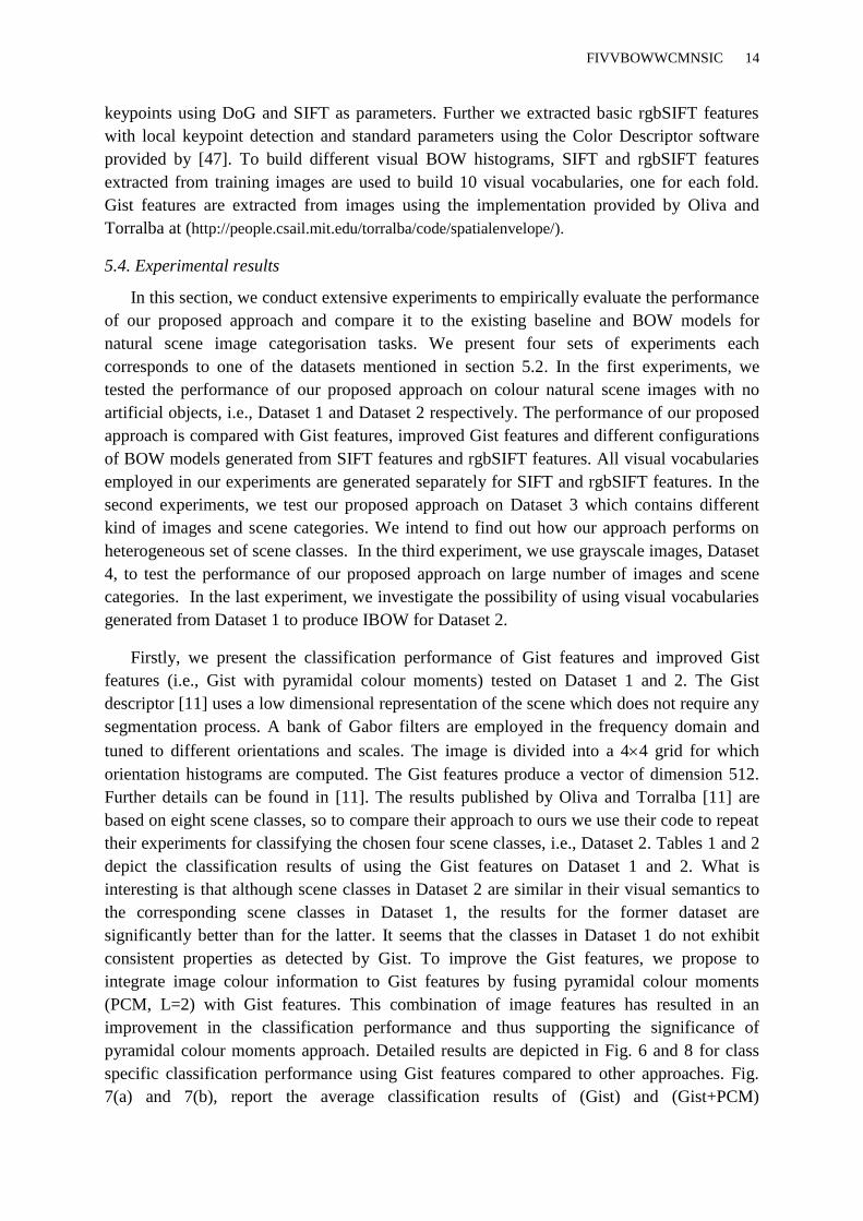
Refer to Fig. 6, it can be seen that our approach works very well in the first three classes,
but the performance degrades for the „open country’ scene class against (Gist+PCM) image
representation. Furthermore, in Fig.8, the performance of our approach on „river/lakes‟ and
FIVVBOWWCMNSIC 16
„sky/clouds‟ scene classes have gained comparable results against other approaches and
outperformed them on the other four classes. The overall performance results of our approach
against other methods are shown in Fig. 7(a) and 7(b).
Fig. 6 The classification performance of IPBOW_PCM compared with different baseline methods for each
scene class of Dataset 2. It is clear that in most scene classes IPBOW_PCM outperforms other methods.
Gist+PCM features perform best for the open country scene class.
Our proposed approach is also compared with colour by design methods. We used
rgbSIFT [47] features, extracted from training images, to generate integrated visual
vocabularies. Each rgbSIFT feature is a vector of 384-D (SIFT features of 128-D are
extracted from RGB image bands respectively). An image is then represented as a histogram
counting the number of keypoints characterised by rgbSIFT that belongs to a specific
vocabulary index. The average of the 10 accuracy rates using 10-fold cross validation is used
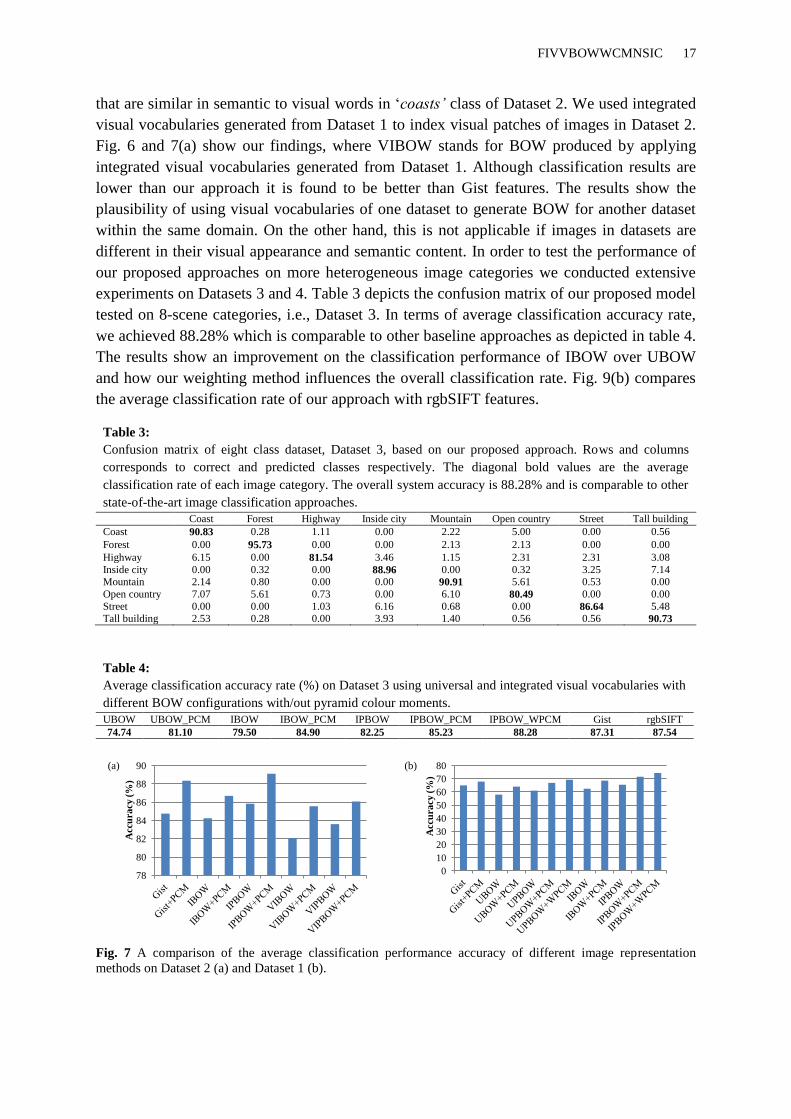
to measure the performance of all experiments as mentioned in section 5.4. Fig. 9(a)
compares the average classification rate of our proposed approach and rgbSIFT features
tested on Dataset 1. The results confirm the effectiveness of our approach compared with
rgbSIFT in image classification task. Our proposed model achieved better results on five
image categories out of 6 while rgbSIFT features performed better in recognising Plains
category.
Moreover, this paper investigates the influence of applying visual vocabularies generated
from one image dataset to generate BOW from another image dataset. We hypothesise that
visual words that exist in a specific image class are similar to those in another class with
same visual semantic features. For example, „coasts' class in Dataset 1 contains visual words
72
76
80
84
88
92
Accu
racy (
%)
Coast
88
90
92
94
96
98
Acc
ura
cy (
%)
Forest
80
82
84
86
88
90
Acc
ura
cy (
%)
Mountain
64
68
72
76
80
84
Acc
ura
cy (
%)
Open country
FIVVBOWWCMNSIC 17
that are similar in semantic to visual words in „coasts’ class of Dataset 2. We used integrated
visual vocabularies generated from Dataset 1 to index visual patches of images in Dataset 2.
Fig. 6 and 7(a) show our findings, where VIBOW stands for BOW produced by applying
integrated visual vocabularies generated from Dataset 1. Although classification results are
lower than our approach it is found to be better than Gist features. The results show the
plausibility of using visual vocabularies of one dataset to generate BOW for another dataset
within the same domain. On the other hand, this is not applicable if images in datasets are
different in their visual appearance and semantic content. In order to test the performance of
our proposed approaches on more heterogeneous image categories we conducted extensive
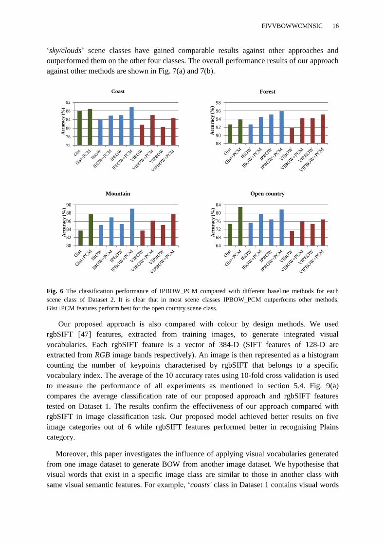
experiments on Datasets 3 and 4. Table 3 depicts the confusion matrix of our proposed model
tested on 8-scene categories, i.e., Dataset 3. In terms of average classification accuracy rate,
we achieved 88.28% which is comparable to other baseline approaches as depicted in table 4.
The results show an improvement on the classification performance of IBOW over UBOW
and how our weighting method influences the overall classification rate. Fig. 9(b) compares
the average classification rate of our approach with rgbSIFT features.
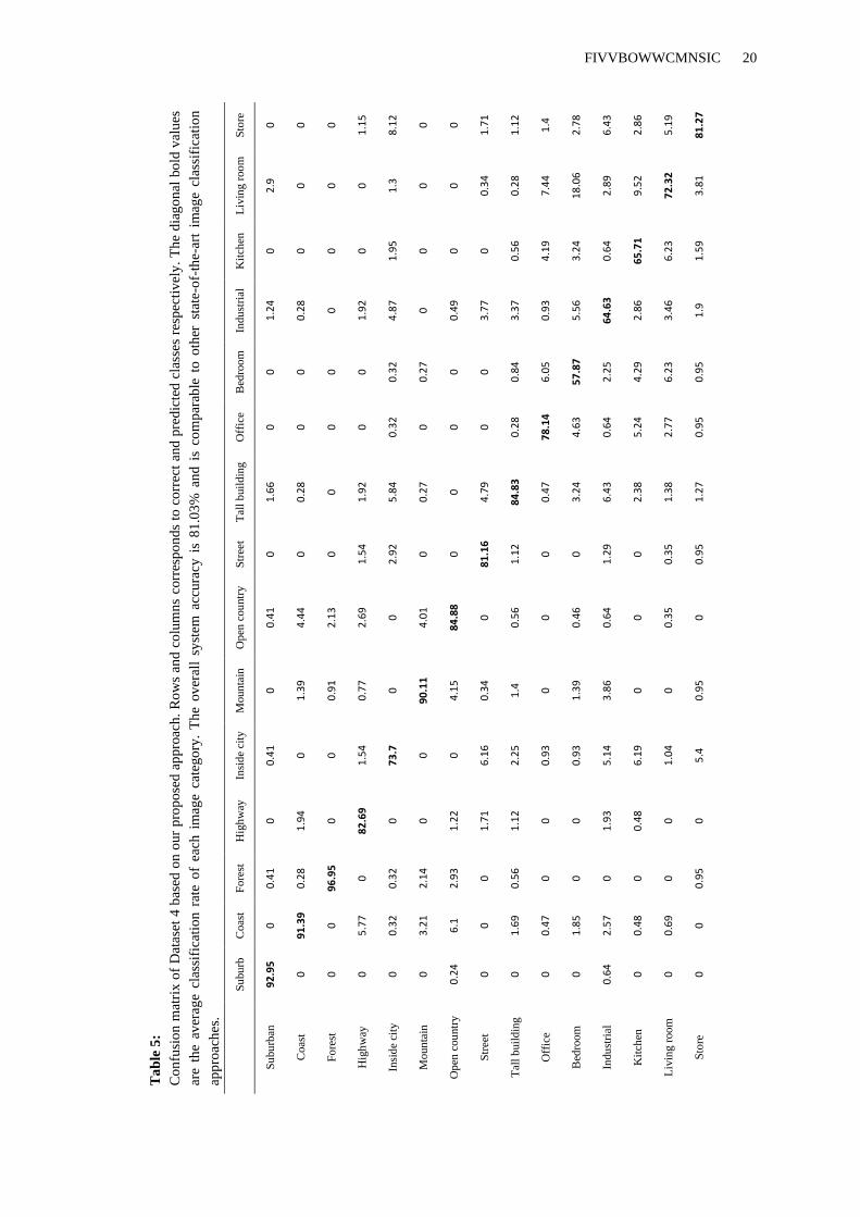
Table 3:
Confusion matrix of eight class dataset, Dataset 3, based on our proposed approach. Rows and columns
corresponds to correct and predicted classes respectively. The diagonal bold values are the average
classification rate of each image category. The overall system accuracy is 88.28% and is comparable to other
state-of-the-art image classification approaches.
Coast Forest Highway Inside city Mountain Open country Street Tall building
Coast 90.83 0.28 1.11 0.00 2.22 5.00 0.00 0.56
Forest 0.00 95.73 0.00 0.00 2.13 2.13 0.00 0.00
Highway 6.15 0.00 81.54 3.46 1.15 2.31 2.31 3.08
Inside city 0.00 0.32 0.00 88.96 0.00 0.32 3.25 7.14 Mountain 2.14 0.80 0.00 0.00 90.91 5.61 0.53 0.00
Open country 7.07 5.61 0.73 0.00 6.10 80.49 0.00 0.00
Street 0.00 0.00 1.03 6.16 0.68 0.00 86.64 5.48 Tall building 2.53 0.28 0.00 3.93 1.40 0.56 0.56 90.73
Table 4:
Average classification accuracy rate (%) on Dataset 3 using universal and integrated visual vocabularies with
different BOW configurations with/out pyramid colour moments.
UBOW UBOW_PCM IBOW IBOW_PCM IPBOW IPBOW_PCM IPBOW_WPCM Gist rgbSIFT
74.74 81.10 79.50 84.90 82.25 85.23 88.28 87.31 87.54
Fig. 7 A comparison of the average classification performance accuracy of different image representation
methods on Dataset 2 (a) and Dataset 1 (b).
78
80
82
84
86
88
90
Acc
ura
cy (
%)
0
10
20
30
40
50
60
70
80
Acc
ura
cy (
%)
(a) (b)

FIVVBOWWCMNSIC 18
Fig. 8 The classification performance of our approach compared with different methods for each scene class of
Dataset 1. It is clear that in most scene classes our approach outperforms other methods.
For Dataset 4, we tested our proposed approach on grayscale images for both training and
testing. In this case, our pyramidal colour moments represents only the information that are
available in single image band i.e., no colour information. First and second moments are
computed from all image sub-regions at pyramidal layout with L=2 and resulted in a vector of
size 42-D. The confusion matrix, depicted in Table 5, illustrate the performance of our
proposed approach. We achieved 81.03% overall classification rate which is higher than
traditional BOW with universal vocabularies. We compared the performance of universal
BOW and integrated BOW with different configurations. Results are reported in Table 6.
Also, our approach is comparable to the results obtained by Battiato et al. [32] where they
achieved 79.43% classification rate on the same dataset.
0 10 20 30 40 50 60 70 80
Acc
ura
cy (
%)
Coast
0
10
20
30
40
50
60
Acc
ura
cy (
%)
River/lake
70
75
80
85
90
95
Acc
ura
cy (
%)
Forest
45
50
55
60
65
70
Acc
ura
cy (
%)
Plain
0
15
30
45
60
75
90
Acc
ura
cy (
%)
Mountain
0
15
30
45
60
75
90
Acc
ura
cy (
%)
Sky_cloud
FIVVBOWWCMNSIC 19
Fig. 9 Performance comparisons between our proposed approach (IPBOW_WPCM) based on SIFT features
and IBOW image representation based on rgbSIFT features [47] both tested on Dataset 1 (a) and Dataset 3
(b).
0 20 40 60 80 100
Coast
River/lake
Forest
Plain
Mountain
Sky/cloud
Classification rate (%)
rgbSIFT IPBOW_WPCM
0 20 40 60 80 100
Coast
Forest
Highway
Insidecity
Mountain
Open country
Street
Tall building
Classification rate (%)
rgbSIFT IPBOW_WPCM (a) (b)
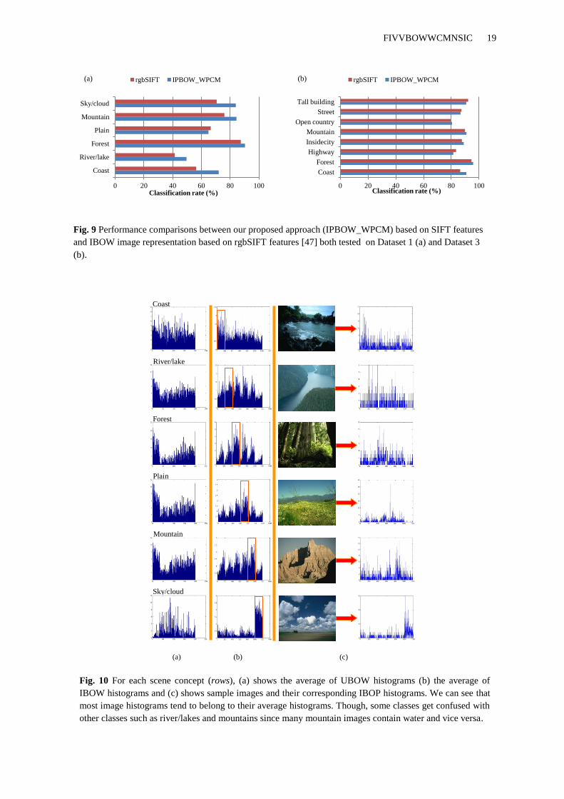
Fig. 10 For each scene concept (rows), (a) shows the average of UBOW histograms (b) the average of
IBOW histograms and (c) shows sample images and their corresponding IBOP histograms. We can see that
most image histograms tend to belong to their average histograms. Though, some classes get confused with
other classes such as river/lakes and mountains since many mountain images contain water and vice versa.
(a) (c) (b)
River/lake
Forest
Plain
Mountain
Sky/cloud
Coast
FIVVBOWWCMNSIC 20
Ta
ble
5:
Co
nfu
sio
n m
atri
x o
f D
atas
et 4
bas
ed o
n o
ur
pro
po
sed a
ppro
ach
. R
ow
s an
d c
olu
mn
s co
rres
po
nd
s to
co
rrec
t an
d p
red
icte
d c
lass
es r
esp
ecti
vel
y.
Th
e d
iag
on
al b
old
val
ues
are
the
aver
age
clas
sifi
cati
on r
ate
of
each
im
age
cate
go
ry.
Th
e ov
eral
l sy
stem
acc
ura
cy i
s 8
1.0
3%
an
d i
s co
mp
arab
le t
o o
ther
st
ate-
of-
the-
art
imag
e cl
assi
fica
tio
n
app
roac
hes
.
Sto
re
0
0
0
1.1
5
8.1
2
0
0
1.7
1
1.1
2
1.4
2.7
8
6.4
3
2.8
6
5.1
9
81
.27
Liv
ing r
oo
m
2.9
0
0
0
1.3
0
0
0.3
4
0.2
8
7.4
4
18
.06
2.8
9
9.5
2
72
.32
3.8
1
Kit
chen
0
0
0
0
1.9
5
0
0
0
0.5
6
4.1
9
3.2
4
0.6
4
65
.71
6.2
3
1.5
9
Indu
stri
al
1.2
4
0.2
8
0
1.9
2
4.8
7
0
0.4
9
3.7
7
3.3
7
0.9
3
5.5
6
64
.63
2.8
6
3.4
6
1.9
Bed
roo
m
0
0
0
0
0.3
2
0.2
7
0
0
0.8
4
6.0
5
57
.87
2.2
5
4.2
9
6.2
3
0.9
5
Off
ice
0
0
0
0
0.3
2
0
0
0
0.2
8
78
.14
4.6
3
0.6
4
5.2
4
2.7
7
0.9
5
Tal
l b
uil
din
g
1.6
6
0.2
8
0
1.9
2
5.8
4
0.2
7
0
4.7
9
84
.83
0.4
7
3.2
4
6.4
3
2.3
8
1.3
8
1.2
7
Str
eet
0
0
0
1.5
4
2.9
2
0
0
81
.16
1.1
2
0
0
1.2
9
0
0.3
5
0.9
5
Op
en c
ou
ntr
y
0.4
1
4.4
4
2.1
3
2.6
9
0
4.0
1
84
.88
0
0.5
6
0
0.4
6
0.6
4
0
0.3
5
0
Moun
tain
0
1.3
9
0.9
1
0.7
7
0
90
.11
4.1
5
0.3
4
1.4
0
1.3
9
3.8
6
0
0
0.9
5
Insi
de
city
0.4
1
0
0
1.5
4
73
.7
0
0
6.1
6
2.2
5
0.9
3
0.9
3
5.1
4
6.1
9
1.0
4
5.4
Hig
hw
ay
0
1.9
4
0
82
.69
0
0
1.2
2
1.7
1
1.1
2
0
0
1.9
3
0.4
8
0
0
Fo
rest
0.4
1
0.2
8
96
.95
0
0.3
2
2.1
4
2.9
3
0
0.5
6
0
0
0
0
0
0.9
5
Coas
t
0
91
.39
0
5.7
7
0.3
2
3.2
1
6.1
0
1.6
9
0.4
7
1.8
5
2.5
7
0.4
8
0.6
9
0
Su
bu
rb
92
.95
0
0
0
0
0
0.2
4
0
0
0
0
0.6
4
0
0
0
Su
bu
rban
Coas
t
Fo
rest
Hig
hw
ay
Insi
de
city
Moun
tain
Op
en c
ou
ntr
y
Str
eet
Tal
l b
uil
din
g
Off
ice
Bed
roo
m
Indu
stri
al
Kit
chen
Liv
ing r
oo
m
Sto
re

FIVVBOWWCMNSIC 21
Table 6 :
Classification results on Dataset 4 using universal and integrated visual vocabularies with different configurations
of BOW to represent visual content.
UBOW UBOW_PCM IBOW IBOW_PCM IPBOW IPBOW_PCM IPBOW_WPCM
Suburban 87.97 88.38 92.95 95.02 91.70 92.95 92.95 Coast 76.11 78.33 84.72 86.39 86.39 88.61 91.39
Forest 91.46 94.21 91.16 93.29 92.68 95.43 96.95
Highway 64.23 70.77 79.62 81.54 78.85 80.77 82.69 Inside city 57.47 62.34 70.45 72.73 70.45 72.08 73.70
Mountain 75.13 78.88 87.17 88.77 87.43 87.17 90.11
Open country 60.00 64.88 76.83 79.76 78.05 79.27 84.88 Street 63.36 71.58 75.34 80.14 76.37 78.08 81.16
Tall building 60.11 65.17 77.25 80.06 80.62 83.43 84.83 Office 68.84 73.95 77.67 80.47 79.07 78.14 78.14
Bedroom 31.02 35.19 55.56 56.48 55.56 57.87 57.87
Industrial 39.87 44.05 52.41 56.59 55.63 57.23 64.63 Kitchen 46.19 50.00 55.71 61.43 62.38 64.29 65.71
Living room 50.52 54.33 57.09 61.25 62.98 67.82 72.32
Store 60.63 67.94 67.94 74.92 69.84 78.10 81.27
Accuracy (%) 63.08 67.56 74.34 77.44 76.05 78.31 81.03
6. Conclusion
In this paper, we have presented a unified framework to classify natural scene images into
one of a number of predefined scene classes. Our work is based on the bag of visual words
(BOW) image representation scheme. The proposed framework improved BOW image
representation model in two ways: (1) It generates discriminative visual vocabularies by
integrating visual vocabularies learned from class-specific data; (2) It fuses image colour
information with intensity-based BOW using a spatial pyramid layout. The fusion has been
done using the keypoints density-based weighting (KDW) method. One of the drawbacks of
using a universal visual vocabulary is that similar visual patches may be clustered into
different clusters and thus loses their information. We investigated different configurations of
BOW and compared their performance on three natural scene datasets. Also, we made an
improvement to the well-known intensity-based Gist features by adding pyramidal colour
moments in an early fusion approach. We have shown that integrated BOW (IBOW) and
pyramidal colour moments (PCM) weighted on spatial pyramid layout (IPBOW+WPCM)
outperformed other baseline approaches. Experimental results showed that building
integrated visual vocabulary provides better performance than the conventional universal
visual vocabulary. Moreover, it is obvious that building integrated visual vocabulary is faster
than universal visual vocabulary, since the clustering algorithm will deal with less feature
vectors and it will probably converge faster. We have also shown that visual vocabularies of
one dataset could be used to generate BOW for another dataset with acceptable classification
performance. We did not focus on weighting BOW visual words since our initial experiments
has shown that BOW weighting techniques such as term-frequency inverse document
frequency (TF-IDF) has gained lower classification performance in our datasets [26]. Further
investigation needs to be done to include feature selection algorithms [48] to reduce the
influence of noisy data. We believe that building visual vocabularies from pyramid regions
could generate better visual vocabularies, leading to more accurate classification and reduces
clustering time. Investigating the effect of colour casting, due to different acquisition
conditions, on image classification task is of possible future work.

FIVVBOWWCMNSIC 22
Acknowledgements
The first author acknowledges the financial support received from the Applied Science University in Jordan. The authors would like to thank Dr. Julia Vogel for providing us access to the natural scene image dataset and for valuable discussion. Also, we would like to thank Dr Paul Trundle for reviewing our paper and for his valuable comments, and the reviewers for their constructive feedback on our work.
References
[1] Y. Rui, T.S. Huang and S.F. Chang, Image retrieval: Current techniques, promising directions, and open
issues. Journal of visual communication and image representation, vol. 10, No. 1, March 1999, pp. 39-62.
[2] Y. Liu, D. Zhang, G. Lu and W.Y. Ma: A survey of content-based image retrieval with high-level semantics.
Pattern Recognition, Vol. 40, No. 1, January 2007, pp. 262-282.
[3] R. Datta, D. Joshi, J. Li, and J.Z. Wang: Image retrieval: Ideas, influences, and trends of the new age. ACM
Computing Surveys, Vol. 40, No. 2, April 2008, pp. 1-60.
[4] J. Vogel, A. Schwaninger, C. Wallraven and H. Bulthoff: Categorization of natural scenes: Local versus
global information and the role of color. ACM Transactions on Applied Perception, Vol. 4, No. 3, November
2007, Article 19.
[5] M.G. Ross and A. Oliva: Estimating perception of scene layout properties from global image features.
Journal of Vision, Vol. 10, No. 1, January 2010, pp. 1-25.
[6] P. Quelhas, F. Monay, J.M. Odobez, D. Gatica-Perez, T. Tuytelaars and L. Van Gool: Modeling scenes with
local descriptors and latent aspects. Proc. of IEEE International Conference on Computer Vision ICCV, Beijing,
China, October 17-21, 2005, pp. 883–890.
[7] J. Vogel and B. Schiele: A semantic typicality measure for natural scene categorization. Lecture notes in
computer science, Vol. 3175, 2004, pp. 195-203.
[8] J.Z. Wang, J. Li and G. Wiederhold: SIMPLIcity: Semantics-sensitive integrated matching for picture
libraries. IEEE Transactions on pattern analysis and machine intelligence, Vol. 23, No. 9, September 2001, pp.
947-963.
[9] A. Vailaya, M.A.T. Figueiredo, A.K. Jain and H.J. Zhang: Image classification for content-based indexing.
IEEE Transactions on Image Processing, Vol. 10, No. 1, January 2001, pp. 117-130.
[10] M. Szummer and R. Picard: Indoor-outdoor image classification. Proc. of IEEE International Workshop on
Content-Based Access of Image and Video Database, Bombay, India, Jan. 1998, pp. 42–51.
[11] A. Oliva and A. Torralba: Modeling the shape of the scene: A holistic representation of the spatial
envelope. International Journal of Computer Vision, Vol. 42, No. 3, May-June 2001, pp. 145-175.
[12] L. Fei-Fei and P. Perona: A bayesian hierarchical model for learning natural scene categories. Proc. of the
IEEE Conference on Computer Vision and Pattern Recognition, CVPR, San Diego, CA, USA, June 20-26,
2005, pp. 524-531
[13] A. Bosch, X. Munoz, A. Oliver and R. Marti: Object and scene classification: what does a supervised
approach provide us. Proc. of the 18th
International Conference on Pattern Recognition, IEEE Computer Society,
ICPR, Hong Kong, China, August 20-24, 2006, pp. 773- 777
[14] A. Bosch, X. Munoz and R. Marti: Which is the best way to organize/classify images by content?. Image
and vision computing, Vol. 25, No. 6, June 2007, pp. 778-791.
[15] P. Quelhas, F. Monay, J.M. Odobez, D. Gatica-Perez and T. Tuytelaars: A thousand words in a scene.
IEEE Transactions on pattern analysis and machine intelligence, Vol. 29, No. 9, August 2007, pp. 1575-1589.
[16] D. Gokalp and S. Aksoy: Scene classification using bag-of-regions representations. Proc. of the IEEE
Conference on Computer Vision and Pattern Recognition, CVPR, Minneapolis, Minnesota, USA, June 18-23,
2007, pp.1-8.
[17] D. Lowe: Distinctive image features from scale-invariant keypoints. International Journal of Computer
Vision, Vol. 60, No. 2, November 2004, pp. 91-110.
[18] P. Quelhas and J. Odobez: Natural scene image modeling using color and texture visterms. Proc. of
International Conference on Image and Video Retrieval, CIVR, Lecture Notes in Computer Science, Tempe,
AZ, USA, July 13-15, 2006, pp. 411-421.
[19] G. Csurka, C. Dance, L. Fan, J. Willamowski and Bray C.: Visual categorization with bags of keypoints.
Proc. of ECCV workshop on Statistical Learning in Computer Vision, Czech Republic, May 11-14, 2004, pp.
59–74.
FIVVBOWWCMNSIC 23
[20] P. Quelhas and J. Odobez: Multi-level local descriptor quantization for bag-of-visterms image
representation. Proc. of the 6th ACM international Conference on Image and Video Retrieval, Amsterdam, The
Netherlands , July 9-11, 2007, pp. 242-249
[21] Z. Wu, Q. Ke, J. Sun and H.Y. Shum: A Multi-Sample, Multi-Tree Approach to Bag-of-Words Image
Representation for Image Retrieval. Proc. of 12th
IEEE International Conference on Computer vision, ICCV,
Kyoto, Japan, September 27 - October 4, 2009, pp. 1992-1999.
[22] D. Nister and H. Stewenius: Scalable recognition with a vocabulary tree. Proc. of IEEE Conference on
Computer Vision and Pattern Recognition CVPR, New York, USA, June 17-22 2006, pp. 2161-2168
[23] F. Perronnin: Universal and adapted vocabularies for generic visual categorization. IEEE Transactions on
pattern analysis and machine intelligence, Vol. 30, No. 7, July 2008, pp. 1243-1256.
[24] J. Wu and J. Rehg: Beyond the Euclidean distance: Creating effective visual codebooks using the histogram
intersection kernel. Proc. of 12th
IEEE International Conference on Computer vision, ICCV, Kyoto, Japan,
September 27 - October 4, 2009, pp.630-637.
[25] Y.G. Jiang, C.W. Ngo and J. Yang: Towards optimal bag-of-features for object categorization and semantic
video retrieval. Proc. of the 6th
ACM international Conference on Image and Video Retrieval, CIVR,
Amsterdam, The Netherlands, July 9-11, 2007, pp. 494-501.
[26] Y. Alqasrawi, D. Neagu and P. Cowling: Natural Scene Image Recognition by Fusing Weighted Colour
Moments with Bag of Visual Patches on Spatial Pyramid Layout. Proc. of the 9th
international Conference on
intelligent Systems Design and Applications, ISDA, IEEE Computer Society, Pisa, Italy, Nov. 30 -Dec. 2 2009,
pp. 140-145.
[27] J. Yang, Y.G. Jiang, A.G. Hauptmann and C.W. Ngo: Evaluating bag-of-visual-words representations in
scene classification. Proc. of the 9th
ACM international Workshop on Multimedia information Retrieval, ACM
MIR, University of Augsburg, Germany, September 28-29, 2007, pp. 197-206.
[28] F. Khan, J. van de Weijer and M. Vanrell: Top-Down Color Attention for Object Recognition. Proc. of 12th
IEEE International Conference on Computer vision, ICCV, Kyoto, Japan, September 27 - October 4, 2009, pp.
979-986.
[29] S. Lazebnik, C. Schmid and J. Ponce: Beyond bags of features: Spatial pyramid matching for recognising
natural scene categories. Proc. of the IEEE Conference on Computer Vision and Pattern Recognition, CVPR,
New York, USA, June 17-22, 2006, pp. 2169-2178.
[30] A. Bosch, A. Zisserman and X. Munoz: Representing shape with a spatial pyramid kernel. Proc. of the 6th
ACM international Conference on Image and Video Retrieval, CIVR, Amsterdam, The Netherlands, July 9-11,
2007, pp. 401-408.
[31] C.H. Lampert, M.B. Blaschko and T. Hofmann: Beyond sliding windows: Object localization by efficient
subwindow search. Proc. of the IEEE Conference on Computer Vision and Pattern Recognition, CVPR,
Anchorage, Alaska, USA, June 24-26, 2008, pp. 1-8.
[32] S. Battiato, G. Farinella, G. Gallo and D. Ravi: Exploiting Textons distributions on spatial hierarchy for
scene classification. EURASIP Journal on Image and Video Processing, special issue on Multimedia Modeling,
January 2010, pp.1-13.
[33] M. Swain and D. Ballard: Color indexing. International Journal of Computer Vision, Vol. 7, No. 1,
November 1991, pp. 11-32.
[34] L. Zhu and A. Zhang: Theory of keyblock-based image retrieval. ACM Transactions on Information
Systems (TOIS), Vol. 20, No. 2, April 2002, pp. 224-257.
[35] J. Sivic and A. Zisserman, Video Google: A text retrieval approach to object matching in videos. Proc. of
the 9th
IEEE International Conference on Computer Vision, ICCV, Nice, France, October 14-17, 2003, pp.
1470– 1477.
[36] F. Jurie and B. Triggs: Creating efficient codebooks for visual recognition. Proc. of 10th
IEEE international
conference on computer vision, ICCV, Beijing, China, October 17-20, 2005, pp. 604-610.
[37] M. Nilsback and A. Zisserman: A visual vocabulary for flower classification. Proc. of IEEE Conference on
Computer Vision, CVPR, New York, USA, June17-22, 2006, 1447-1454.
[38] J.C. van Gemert, C.G.M. Snoek, C.J. Veenman, A.W.M. Smeulders and J.M. Geusebroek: Comparing
compact codebooks for visual categorization. Computer Vision and Image Understanding, Vol 114, No. 4, April
2010, pp. 450-462.
[39] Y.G. Jiang, J. Yang, C.W. Ngo and A.G. Hauptmann: Representations of keypoint-based semantic concept
detection: A comprehensive study. IEEE Transactions on Multimedia, Vol. 12, No. 1, January 2010, pp. 42-53.
[40] K. Mikolajczyk and C. Schmid: A performance evaluation of local descriptors. IEEE Transactions on
pattern analysis and machine intelligence, October 2005, pp. 1615-1630.
[41] http://lear.inrialpes.fr/people/mikolajczyk/.
[42] F. Odone, A. Barla and A. Verri: Building kernels from binary strings for image matching. IEEE
Transactions on Image Processing, Vol. 14, No. 2, February 2005, pp. 169-180.

FIVVBOWWCMNSIC 24
[43] C.-C. Chang, and Ling, C.-J., LIBSVM: a library for support vector machines. Software available at:
http://www.csie.ntu.edu.tw/~cjlin/libsvm/, 2001.
[44] Alessandro Perina, Marco Cristani, Vittorio Murino: Learning natural scene categories by selective multi-
scale feature extraction. Image and Vision Computing, Vol 28, No. 6, June 2010, pp. 927-939.
[45] G. Farinella, S. Battiato: Representation Models and Machine Learning Techniques for Scene
Classification. Chapter in Pattern Recognition, Machine Vision, Principles and Applications, Ed. PSP Wang,
River publisher, Denmark, chapter 13, 2010 pp. 199-214.
[46] Battiato, S. and Farinella, G.M. and Guarnera, G.C. and Meccio, T. and Puglisi, G. and Ravi, D. and Rizzo,
R.: Bags of phrases with codebooks alignment for near duplicate image detection. Proc. of the 2nd
ACM
workshop on Multimedia in forensics, security and intelligence, Firenze, Italy, October 25-29, 2010, pp. 65-70.
[47] Koen E. A. van de Sande, Theo Gevers and Cees G. M. Snoek: Evaluating Color Descriptors for Object
and Scene Recognition. IEEE Transactions on Pattern Analysis and Machine Intelligence, Vol. 32, No. 9,
September 2010, pp. 1582-1596.
[48] E. Guldogan and M. Gabbouj: Feature selection for content-based image retrieval. Journal of Signal, Image
and Video Processing, Springer, Vol. 2, No. 3, September, 2008, pp. 241-250.


