1
ANALYSIS OF REPEATED ICESAT FULL WAVEFORM DATA: METHODOLOGY AND
LEAF-ON / LEAF-OFF COMPARISON
Hieu Duong1
Norbert Pfeifer2
Roderik Lindenbergh1
1: DEOS, MGP-FRS, 2: University of Innsbruck, Institute of Geography

2
Outline
• Introduction• ICESat/GLAS.• Waveform groundtracks in study area
• Waveform processings• Results and Discussion.• Conclusion
3
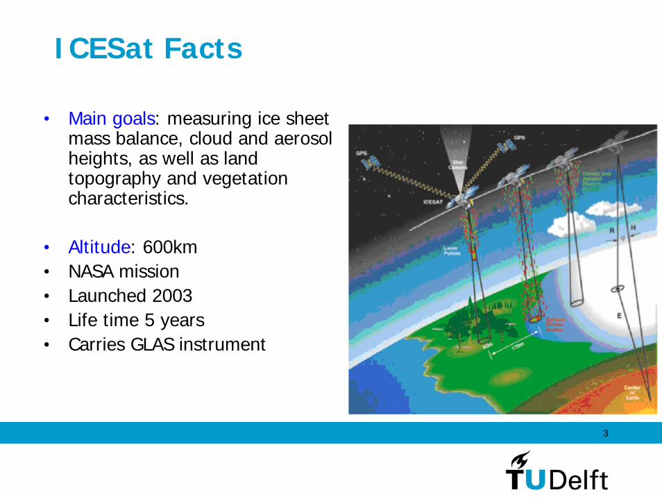
ICESat Facts
• Main goals: measuring ice sheet mass balance, cloud and aerosol heights, as well as land topography and vegetation characteristics.
• Altitude: 600km• NASA mission• Launched 2003• Life time 5 years• Carries GLAS instrument
4
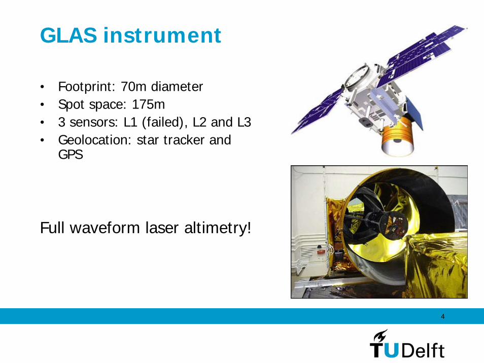
GLAS instrument
• Footprint: 70m diameter• Spot space: 175m• 3 sensors: L1 (failed), L2 and L3• Geolocation: star tracker and
GPS
Full waveform laser altimetry!

5
ICESat repeated tracks
February:1840 waveforms
September:2942 waveforms
Forest pairs:358

6
ICESat repeated tracks
• Green: February 2003• Red: September 2003
40 60 80 1000
10
20
30
40
50Histogram of footprint shift
← mean =73.86[m]
• Select forest footprints manually by comparing to Landsat images.

7
Target: detect waveform changes
Fitting algorithm
Waveform Normalization
Conversion-Bin-ASCII-Counts-Voltage
-Smoothing-Initial parameters estimation
Shifting Computation
Waveform Distances-> DI, Intensity Dist-> RP, Peak Ratio
25% smallest RP & DI
-> C_DI threshold-> C_RP threshold
GLA01
GLA14
Extraction of ELevation
Points by IDL
8
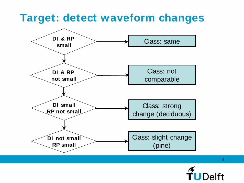
Target: detect waveform changes
Class: sameDI & RP small
Class: not comparable
DI & RP not small
DI smallRP not small
DI not smallRP small
Class: slight change (pine)
Class: strong change (deciduous)
9
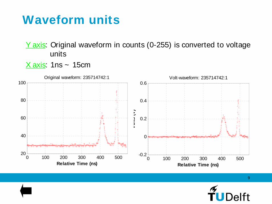
Waveform units
Y axis: Original waveform in counts (0-255) is converted to voltage units
X axis: 1ns ~ 15cm
0 100 200 300 400 50020
40
60
80
100Original waveform: 235714742:1
Relative Time (ns)0 100 200 300 400 500
-0.2
0
0.2
0.4
0.6Volt-waveform: 235714742:1
Volts
(V)
Relative Time (ns)

10
Normalization
Total intensity: ∑=
544
1iiV
=> Normalization step:
∑=
= 544
1ii
inori
V
VV
Area under waveform equals to 1.
After that we smooth the waveform.
Mean total intensity February: 116.48September: 39.90

11
Fitting: Gaussian decomposition
• Transmitted pulse is in Gaussian model• Return waveform is a sum of Gaussian components• Fitting algorithm: least square estimation
(Vienna Univ. of Tech.)

12
Results of Gaussian decompositionRed: raw waveformGreen: Gaussian components
First mode: left most Gaussian componentLast mode: right most
0 200 400 600-0.01
0
0.01
0.02
0.03
0.04Myfit-date:27-02-2003-49338080:19
Relative Time (ns)0 200 400 600
-0.01
0
0.01
0.02
0.03
0.04Myfit-date:30-09-2003-235714742:1
Relative Time (ns)

13
Shift
Blue: winter waveformRed: summer waveformGreen: shifted winter waveform
0 100 200 300 400 500 600-0.01
0
0.01
0.02
0.03
0.04
0.05
0.06
0.07Waveform:27-02-2003<->30-09-2003
Nor
Volts
(V)
Relative Time (ns)
27-02-2003: in winter30-09-2003: in summer27-02-2003:shifted in winter
The average shift of 4.26[m] maybe caused by changes in the GLASconfiguration
-400 -200 0 200 4000
10
20
30
40
50X: -28.5Y: 50

14
Waveform distances
Intensity distance:
Along vertical axis
Along horizontal axis
Peak ratio:
2544
1
( ( ) ( ))( , )
544F S
F Si
V i V iDI W W
=
−= ∑
1,( , )
1,
F FF F S S
S SF S
S SF F S S
F F
LM FMLM FM LM FM
LM FMRP W W
LM FMLM FM LM FM
LM FM
−⎧− − > −⎪ −⎪= ⎨ −⎪ − − ≤ −⎪ −⎩

15
Waveform parameters
Peak locations• last mode ~ ground surface• first mode ~ canopy top
Widths of modes:~ feature roughness or slope surface, or both, canopy thickness
Amplitudes of modes• first mode ~ canopy density
Distance first-last mode~ tree height
0 200 400 600-0.005
0
0.005
0.01
0.015
0.02
0.025y
Relative Time (ns)

16
Mean parameter valuesFirst mode width• February: 4.28m• September: 3.74m
First mode amplitude• February: 0.00418• September: 0.0056
Last mode amplitude• February: 0.0083• September: 0.0088
First-Last peak distance• February: 20.41m• September: 19.18m
0 0.01 0.02 0.03 0.040
20
40
60
80
100Histogram of amplitude of first mode in February
← mean =0.0041892
0 0.01 0.02 0.03 0.040
20
40
60
80Histogram of amplitude of f irst mode in September
← mean =0.005615

17
Results: Waveform classes
0 200 400 6000
0.01
0.02
0.03
0.04same: 49338080-19<>235714742-1
wintersummer
0 200 400 600
0
5
10
15
20x 10-3
pine forest: 49337720-20<>235714382-2
wintersummer
0 200 400 600
0
0.01
0.02
0.03deciduous f orest49338120-36<>235714782-18
wintersummer
0 200 400 600
0
5
10
15
x 10-3 not comparable:49337780-20<>235714442-2
wintersummer
20 pairs
small-small
70 pairs
small-not small: deciduous?
69 pairs
not small-small
199 pairs
not small-not small

18
Conclusion
• Possible to compare repeated track ICESat waveform data, but, standardization steps are needed.
• Standardization steps, waveform parametrizations and waveform distances can be applied to non-ICESat waveform data as well.
• Waveform processing procedure should be extended, and tested more extensively on a more controlled data set.

19
Upcoming
• Article on land cover classification via analyzing ICESat’s full waveform data
(ISPRS Symposium, Enschede, May 2006)


