
From Desktop to Benchtop – Developing
Computational Tools for Organic and Medicinal
Chemistry
Mihai Burai-Patrascu
A thesis submitted to McGill University in partial fulfillment of the requirements
for the degree of Doctor of Philosophy.
Department of Chemistry
McGill University
Montréal, Québec, Canada
April 2020
© Mihai Burai-Patrascu, 2020

ii
Abstract
Organic and medicinal chemistry research contribute extensively to the discovery,
optimization, and ton-scale production of numerous small molecules, such as novel drugs that treat
life-threatening diseases. This research can be put in the context of the COVID-19 global
pandemic, which has claimed many lives, shut down the entire planet, and made humanity reliant
on chemistry (amongst which organic and medicinal chemistry play a key role) and biochemistry
research to come up with innovative solutions in a short amount of time. A major hurdle in organic
and medicinal chemistry research is the production of these complex life-saving small molecules
and the tedious and time-consuming syntheses they require. To offset this, these two fields of
chemistry make use of a different branch of chemistry, namely computational chemistry. Over the
years, computational chemistry has become a trusted partner of experimental chemistry and has
significantly contributed to the discovery of novel drugs. However, computational chemistry often
requires expertise in both chemistry and coding, the latter of which most experimentalists do not
possess. As such, in this thesis I seek to develop and interface computational tools with organic
and medicinal chemistry to improve the molecular discovery rate. The majority of the tools that
we have developed have been implemented in our drug discovery platform FORECASTER and in
our asymmetric catalyst design platform VIRTUAL CHEMIST, to enable chemists to use powerful
software developed by chemists for chemists. In only a few clicks, the user can interact with our
platforms without the need for expertise in computational chemistry.
This thesis begins with a short but comprehensive introduction (Chapter 1) into
computational chemistry and its various applications. Following this, I developed a computational
protocol that allows the accurate modeling of nucleoside conformations (Chapter 2), which in turn

iii
enables the synthesis of only those nucleosides that exhibit desirable properties. This work was
done in relation to the current methodology of developing nucleosides, which entails the synthesis
of multiple analogues until one with desirable properties is found, since this contributes to an
increased cost, waste production and energy expenditure. Then, using this protocol, I quantified
the various effects that contribute to the different nucleoside conformations, and we were able to
provide plausible explanations of why non-natural nucleosides behave in certain ways (Chapter
3). As a change of pace, I turned my attention to Cytochrome P450-mediated drug metabolism and
toxicity, which constitutes one of the main interests of medicinal chemists (Chapter 4). In this
chapter I developed a novel tool based on quantum mechanics, docking and machine learning that
enables the identification of Cytochrome P450 inhibitors in silico. This allows medicinal chemists
to test whether a compound or drug of interest presents inhibitory activity against a Cytochrome
P450 isoform before attempting synthesis. Finally, we provided organic chemists with a
computational platform – VIRTUAL CHEMIST – that allows them to undertake an asymmetric
synthesis project virtually from A-Z (Chapter 5). Such a platform facilitates organic chemists to
test thousands of molecules at the click of a button and to select only those catalysts that show
excellent stereoselectivity and reactivity. The thesis then concludes with the overall obstacles I
have overcome in my research, as well as possible future avenues for research.

iv
Résumé
La recherche en chimie organique et médicinale contribue largement à la découverte, à
l'optimisation et à la production à l'échelle de la tonne de nombreuses petites molécules, telles que
les nouveaux médicaments qui traitent des maladies mortelles. Cette recherche peut être placée
dans le contexte de la pandémie mondiale COVID-19, qui a fait de nombreuses victimes, a fermé
la planète entière et a rendu l'humanité dépendante de la capacité de la recherche en chimie
(organique et médicinale) et biochimie à trouver des solutions innovantes en peu de temps pour
ceux qui en ont besoin. L'un des principaux obstacles à la recherche en chimie organique et
médicinale est la production de ces petites molécules complexes qui sauvent des vies et le
développement des synthèses fastidieuse qu'elles nécessitent souvent. Pour y remédier, ces deux
domaines de la chimie font appel à une branche différente de la chimie, à savoir la chimie
computationnelle. Au fil des ans, la chimie computationnelle est devenue un partenaire de
confiance de la chimie expérimentale et a contribué de manière significative à la découverte de
nouveaux médicaments. Cependant, la chimie computationnelle requiert souvent une expertise à
la fois en chimie et en programmation, cette dernière n'étant pas du ressort de la plupart des
expérimentateurs. C'est pourquoi, dans cette thèse, nous cherchons à développer et interfacer les
outils informatiques avec la chimie organique et médicinale afin d'améliorer le taux de découverte
moléculaire. La majorité des outils que nous avons développés ont été intégrés dans notre
plateforme de découverte de médicaments FORECASTER, et dans notre plateforme de conception
de catalyseurs asymétriques VIRTUAL CHEMIST, pour permettre aux chimistes d'utiliser des
logiciels puissants développés par des chimistes pour des chimistes, qui peuvent être utilisés en
quelques clics seulement, sans avoir besoin d'une expertise en chimie computationnelle.

v
Dans l'ensemble, cette thèse commence par une introduction complète mais concise
(Chapitre 1) à la chimie computationnelle et à ses diverses applications. Ensuite, nous présentons
un protocole de calcul que nous avons développé et qui permet la modélisation précise des
conformations de nucléosides (Chapitre 2), qui à son tour permet la synthèse des seuls nucléosides
qui présentent des propriétés souhaitables. Ce travail a été effectué en relation avec la
méthodologie actuelle de développement des nucléosides, qui implique la synthèse de multiples
analogues jusqu'à ce qu'un seul présentant des propriétés souhaitables soit trouvé. La synthèse
d'analogues multiples contribue à augmenter les coûts, la production de déchets et la dépense
énergétique. Ensuite, grâce à ce protocole, nous avons quantifié les divers effets qui contribuent
aux différentes conformations des nucléosides, et nous avons pu fournir des explications plausibles
sur les raisons pour lesquelles des nucléosides non naturels se comportent de certaines manières
(Chapitre 3). Par la suite, nous avons porté notre attention sur le métabolisme et la toxicité des
médicaments par les cytochromes P450, qui constituent l'un des principaux intérêts des chimistes
médicinaux (Chapitre 4). Dans ce chapitre, nous avons développé un nouvel outil basé sur la
mécanique quantique, l'arrimage et l'apprentissage machine qui permet l'identification in silico des
inhibiteurs de cytochromes P450. Cela permet aux chimistes de tester si un composé ou un
médicament d'intérêt présente une activité inhibitrice contre une isoforme des cytochromes P450,
sans avoir besoin de synthèses coûteuses ou d'acheter des kits de test. Enfin, nous nous efforçons
de fournir aux chimistes organiciens une plateforme de calcul - VIRTUAL CHEMIST - qui leur permet
d'entreprendre un projet de synthèse asymétrique virtuellement de A à Z (Chapitre 5). Une telle
plateforme permet aux chimistes organiciens de tester des milliers de molécules en un clic et de
ne sélectionner que les catalyseurs qui présentent une excellente stéréosélectivité et réactivité. La

vi
thèse se termine ensuite par les obstacles que nous avons surmontés dans nos recherches, ainsi que
les développements futurs de nos travaux.

vii
Acknowledgements
First of all, I would like to thank my supervisor, Dr. Nicolas Moitessier, for his
unwavering support, mentorship and friendship during my PhD. Brainstorming sessions, code
implementations, fixing memory leaks, petting dogs in the office, Zoom meetings, getting
overpriced and tasteless Tim Horton’s coffee, you name it, we did it. Also, lest we forget – backing
up your code is essential, if you do not want to spend thousands of $$$ to recover it from a 15-
year old HDD. I would also like to thank my family – you were always there for me and I couldn’t
have done it without you. Mulţumesc! I would also like to thank my roommate and BFF Patrick
Outhwaite for putting up with me for 4 years – I have no idea how I would have stayed sane
during my PhD without watching the Premier League and supporting Crystal Palace (which you
made me a fan of). Also ordering food, taking care of dogs together and watching Impractical
Jokers and laughing so much that I would stop breathing … also of course being
QUARANTINED together during a pandemic. I want to thank Sharon Pinus – I have to admit, I
didn’t really like you at the beginning, but you soon turned into one of my favorite people ever.
You made my days in the office so much better, including but not limited to Haribo, cookies,
Hamantaschen and stories of Israel and Germany. Our daily ritual of looking at the “Rate My
Dogs” dog of the day was something I always looked forward to. Thank you! I also want to thank
Julia Stille and Anne Labarre. Our lengthy discussions of what constitutes a sandwich, camping
trip(s), mojito nights and asking me to provide you with the admin password to install software on
your PC kept me sane during this degree. I’m lucky to have you and Sharon as such good friends
– thank you! Another major thank you goes to the Moitessier Research Group – past and present.
I learnt so much from y’all and I hope I was able to impart some of my knowledge and passion on
you. I couldn’t have asked for a better environment to do my PhD in, thank you! Last, I would like

viii
to thank Ginger, Darcy, Jack, Leia and Gaia (and their owners) – amazing dogs I had the
opportunity and pleasure to spend time with and take care of. You hold a special place in my heart.
For those of you I haven’t mentioned in this short acknowledgment section – I haven’t forgotten
you - you are forever in my heart!

ix
Table of Contents
Chapter 1 – Introduction ............................................................................................ 1
1.1. Computational Chemistry – A Brief History. .................................................................. 1
1.2. Computational Techniques – An Overview. .................................................................... 2
1.2.1. Molecular Mechanics (MM). .................................................................................... 2
1.2.1.1. MM – Force Field Energy Terms. ..................................................................... 3
1.2.1.2. MM – Force Field Atom Types. ........................................................................ 5
1.2.1.3. MM - Applications. ........................................................................................... 6
1.2.1.4. MM - Limitations. ............................................................................................. 7
1.2.2. Quantum Mechanics (QM). ...................................................................................... 8
1.2.2.1. Hartree-Fock (HF). ............................................................................................ 8
1.2.2.1.1. HF - Background. .......................................................................................... 8
1.2.2.1.2. HF - Limitations. ......................................................................................... 10
1.2.2.1.3. HF - Applications. ....................................................................................... 10
1.2.2.2. Semiempirical Methods (SE-QM). .................................................................. 11
1.2.2.2.1. SE-QM - Background. ................................................................................. 11
1.2.2.2.2. SE-QM - Limitations. .................................................................................. 12
1.2.2.2.3. SE-QM - Applications. ................................................................................ 12
1.2.2.3. Density Functional Theory (DFT). .................................................................. 13
1.2.2.3.1. DFT - Background. ...................................................................................... 13
1.2.2.3.2. DFT - Limitations. ....................................................................................... 15
1.2.2.3.3. DFT - Applications. ..................................................................................... 15
1.2.3. Quantum Mechanics/Molecular Mechanics (QM/MM). ........................................ 19
1.2.4. Machine Learning (ML). ........................................................................................ 21
1.2.4.1. ML – Background. ........................................................................................... 21
1.2.4.2. ML - Artificial Neural Networks. .................................................................... 22
1.2.4.3. ML - Random Forest Models. ......................................................................... 24
1.2.4.4. ML – Limitations. ............................................................................................ 26
1.3. Computational Tools in the Context of Medicinal Chemistry and Drug Discovery. ..... 26
1.3.1. Computer-Aided Drug Design (CADD). ................................................................ 27
x
1.3.1.1. Structure-Based Drug Design (SBDD). ........................................................... 27
1.3.1.1.1. SBDD - Molecular Docking. ....................................................................... 28
1.3.1.1.2. SBDD - Virtual Screening. .......................................................................... 29
1.3.1.1.3. SBDD - MD Simulations. ............................................................................ 30
1.3.1.2. Ligand-Based Drug Design (LBDD). .............................................................. 32
1.3.1.2.1. LBDD – QSAR. ........................................................................................... 32
1.3.1.2.2. LBDD - Pharmacophore Modeling. ............................................................ 33
1.4. Computational Tools in the Context of Organic Chemistry. ......................................... 35
1.4.1. Reaction Mechanisms. ............................................................................................ 36
1.4.2. Chemical Reactivity. ............................................................................................... 40
1.4.3. Catalyst Design, Screening and Enantioselectivity Computations. ........................ 43
1.5. Conclusions. ................................................................................................................... 48
1.6. Thesis Objectives. .......................................................................................................... 50
Chapter 2 – Accurately Modeling the Conformational Preferences of Nucleosides –
Methodology ............................................................................................................51
Preface. ...................................................................................................................................... 51
Abstract. .................................................................................................................................... 52
2.1. Introduction. ................................................................................................................... 53
2.1.1. Chemically Modified Oligonucleotides. ................................................................. 53
2.1.2. Nucleoside Reverse Transcriptase Inhibitors (NRTIs). .......................................... 53
2.1.3. Nucleoside Conformation. ...................................................................................... 54
2.1.4. Computational Methods. ......................................................................................... 57
2.2. Benchmark Study. .......................................................................................................... 58
2.2.1. DFT Calculations. ................................................................................................... 59
2.2.2. MM Study. .............................................................................................................. 60
2.2.3. QM/MM Calculations. ............................................................................................ 63
2.3. Validation of the Method on a Set of Nucleosides and Monosaccharides. .................... 64
2.3.1. Application to Monosaccharides Investigations. .................................................... 65
2.3.2. Application to Nucleosides Investigations. ............................................................. 70
2.3.3. Nucleosides – Stereoelectronic Effects. .................................................................. 72
2.4. Conclusions. ................................................................................................................... 77
2.5. Methods. ......................................................................................................................... 77

xi
2.5.1. Initial DFT Study. ................................................................................................... 77
2.5.2. QM/MM/MD Study. ............................................................................................... 78
2.5.3. Umbrella Sampling Simulations. ............................................................................ 79
2.5.4. Natural Bond Orbital (NBO) Analysis. .................................................................. 80
2.5.5. Molecular Orbital Analysis. .................................................................................... 80
2.5.6. Crystal Structures. ................................................................................................... 80
Chapter 3 – Accurately Modeling the Conformational Preferences of Nucleosides –
Applications .............................................................................................................81
Preface. ...................................................................................................................................... 81
Abstract. .................................................................................................................................... 82
3.1. Introduction. ....................................................................................................................... 83
3.2. Effect of Fluorine and Methoxy Substituents on Nucleoside Puckering. .......................... 85
3.2.1. NMR Spectroscopy...................................................................................................... 85
3.2.2. Predicted N/S Ratios and Lowest Energy Structures. .................................................. 87
3.2.3. Quantifying Stereoelectronic Effects. .......................................................................... 89
3.2.4. Comparing Computed and Crystal Structures. ............................................................ 91
3.3. Atypical Fluorine-Hydrogen Bonds and Their Effects on Nucleoside Conformations. .... 94
3.3.1. Nucleosides That Can Potentially Exhibit Fluorine-Hydrogen Bonds. ....................... 95
3.3.2. Analysis of Nucleosides 3.10-3.13. ............................................................................. 96
3.3.3. Analysis of Nucleoside 3.14. ....................................................................................... 99
3.4. Conclusions. ..................................................................................................................... 103
3.5. Methods. ........................................................................................................................... 103
Chapter 4 – Predicting Cytochrome P450 Inhibition and Metabolism at the Drug
Development Stage ................................................................................................105
Preface. .................................................................................................................................... 105
Abstract. .................................................................................................................................. 106
4.1. Introduction. ................................................................................................................. 107
4.2. Drug Metabolism, Bioactivation and Toxicity. ............................................................ 107
4.3. CYP Inhibition - Background. ..................................................................................... 109
4.4. CYP Inhibition – Model Development – Preview. ...................................................... 113
4.4.1. CYP Inhibition – Model Development – QM – Step 1. ....................................... 114
4.4.2. CYP Inhibition – Model Development – QM – Step 2. ....................................... 116

xii
4.4.3. CYP Inhibition – Model Development – Docking – Step 1. ................................ 119
4.4.4. CYP Inhibition – Model Development – Docking – Step 2. ................................ 121
4.4.5. CYP Inhibition – Model Development – ANN – Steps 1 and 2. .......................... 126
4.4.6. CYP Inhibition – Model Development – ANN – Step 3. ..................................... 128
4.4.7. CYP Inhibition – Model Development – ANN – Step 4. ..................................... 130
4.5. SoM Prediction – IMPACTS 2.0 – Background. ............................................................ 131
4.5.1. SoM Prediction – Improving IMPACTS – Approach. ............................................. 132
4.5.2. SoM Prediction – Improving IMPACTS – Ligand Reactivity. ................................ 134
4.5.3. SoM Prediction – Improving IMPACTS – New Activation Energies. .................... 136
4.5.4. SoM Prediction – Improving IMPACTS – Steric Effects and Ligand Accessibility.
138
4.5.5. SoM Prediction – Improving IMPACTS – IMPACTS 2.0. ........................................ 139
4.5.6. SoM Prediction – Improving IMPACTS – IMPACTS 2.0 – Protein Flexibility. ........ 140
4.6. Conclusions. ................................................................................................................. 142
4.7. Methods. ....................................................................................................................... 143
Chapter 5 – From Desktop to Benchtop – A Paradigm Shift in Asymmetric
Synthesis ................................................................................................................145
Preface. .................................................................................................................................... 145
Abstract. .................................................................................................................................. 147
5.1. Introduction. ..................................................................................................................... 148
5.2. Asymmetric Synthesis and Stereoselectivity Prediction. ................................................. 149
5.3. Challenges and Methodologies. ....................................................................................... 150
5.3.1. Preparation of Libraries of Catalysts. ........................................................................ 153
5.3.2. Predicting Enantioselectivities. ................................................................................. 153
5.3.2.1. Preparing the TSs for Enantioselectivity Computations. .................................... 154
5.3.2.2 ACE. ...................................................................................................................... 155
5.3.2.3. QUEMIST. ............................................................................................................. 156
5.3.3. Evaluating Catalytic Activity. ................................................................................... 162
5.4. Validation of the Platform. ............................................................................................... 164
5.4.1. Scenario #1 – One by One Design............................................................................. 164
5.4.2. Scenario #2 – Novel Chemical Series. ...................................................................... 168
5.4.3. Scenario #3 – Virtual Analogue Search. ................................................................... 171
5.4.4. Scenario #4 – Catalyst Substrate Scope. ................................................................... 173

xiii
5.5. Reproducibility. ................................................................................................................ 174
5.6. Conclusions. ..................................................................................................................... 175
Chapter 6 – Conclusions and Future Work ............................................................177
Appendix A ............................................................................................................184
Appendix B ............................................................................................................216
Appendix C ............................................................................................................220
Appendix D ............................................................................................................254
Chapter 7 – References ..........................................................................................282

xiv
List of Figures
Figure 1.1. Molecular structure: Clobazam.13 Arrows: orange – bond stretching; black – angle
bending; yellow – torsional rotation; green – electrostatic interactions; blue – vdW interactions;
oop angle bending not shown for clarity. ........................................................................................ 4
Figure 1.2. The atom type assigned to the aromatic carbon depicted in red would be the same for
all three cases, irrespective of the substituent nature. ..................................................................... 6
Figure 1.3. Structure of derriobtusone A (left). Comparison between the experimental and
predicted Raman spectra (middle) and IR spectra (right) for derriobtusone A. Spectra taken from
reference 49. .................................................................................................................................. 16
Figure 1.4. Reaction mechanism in acetonitrile of the selenium organocatalyzed syn-
dichlorination of 2-pentene using PhSeCl as the active catalytic species. The reaction is endergonic
by ~ 17 kcal/mol. Figure reproduced from reference 51. ............................................................. 17
Figure 1.5. Reaction mechanism in acetonitrile of the selenium organocatalyzed syn-
dichlorination of 2-pentene using PhSeCl3 as the active catalytic species. The reaction is exergonic
by ~ 45 kcal/mol. Figure reproduced from reference 51. ............................................................. 17
Figure 1.6. Hydrogen bonding interactions between the urea catalyst and styrene oxide. Key
interactions are shown with dashed red lines. Figure reproduced from reference 52. .................. 19
Figure 1.7. Description of a simple ANN containing an input and output layer along with neurons
and synapses.................................................................................................................................. 24
Figure 1.8. Decision tree describing whether a drug candidate would be kept or discarded based
on its logP value. ........................................................................................................................... 25
Figure 1.9. Structure of Clobazam13 (left) and its pharmacophore (right). Red – halogen moiety;
blue – aromatic moiety; green – hydrogen bond acceptor; purple – hydrophobic moiety. .......... 34
Figure 1.10. Structures of p-coumarol, coniferol and sinapol. .................................................... 42
Figure 1.11. Structures of the enolate ions of cyclohexanone, phenacyl and butyrolactone. ...... 42
Figure 1.12. Top: Hammond-Leffler postulate: the TS resembles the reactants (A) if it is an early
TS and the products (B) if it is a late TS. The step λ controls whether the TS is late or early in the
ACE computations. Bottom: Schematic depiction of the Curtin-Hammet principle.
Stereoselectivity of a catalyst can be computed by converting the difference in energy between
TS1 and TS2 (i.e. ∆∆G‡) to an enantiomeric excess (%ee) ratio. .................................................. 47
Figure 2.1. Nucleoside analogues used as drugs. ......................................................................... 54
Figure 2.2. a) Conformational characterization of the ribose puckering;150 b) 2’-F,4’-OMe-rU
(2.8)151 and clinically-relevant nucleoside analogues. .................................................................. 55
Figure 2.3. Definition of dihedral angles used to calculate the pseudorotational phase angle P in
Eqs. 2.1 and 2.2. R = any substituent. ........................................................................................... 56
Figure 2.4. a) PMF curve along the pseudorotational phase angle for 2.8 using GLYCAM. Inset
shows the sugar pucker distribution. (blue – N, green – S). b) PMF curves obtained using the RM1,

xv
PM3 and PM3CARB1 semi-empirical methods. c) Exocylic C4-C5 bond rotation was shown to
be on a faster time scale than sugar puckering.162 d) PMF curve of 2.8 using SCC-DFTB. Inset
shows the sugar pucker distribution (blue – N, green – S)............................................................ 62
Figure 2.5. Structural information for the N and S minima obtained for 2.8.151 .......................... 64
Figure 2.6. Superposition of the crystal structures and lowest-in-energy predicted conformers of
2.9, 2.11, 2.12, 2.15 and 2.16 (pink – computed structure, green – crystal structure). ................. 68
Figure 2.7. Anomeric and gauche effects observed after the NBO analysis for 2.8. Relative
energies are given in kcal/mol. ..................................................................................................... 73
Figure 2.8. PMF curve for nucleoside 2.28. Inset shows the sugar puckering distribution along the
pseudorotational angle P. .............................................................................................................. 74
Figure 2.9. Intramolecular hydrogen bonds for the North pucker (a) and South pucker (b) for 2.30.
a) hydrogen bonding between C=O-H2’ and C=O-2’OH. b) hydrogen bonding between O5-
H(base). ......................................................................................................................................... 76
Figure 3.1. Definition of J coupling constants used in experimentally determining N/S equilibrium.
....................................................................................................................................................... 84
Figure 3.2. Computed lowest energy structures for A. N conformations: left – 3.2; center – 3.3;
right – 3.8 and B. S conformations: left – 3.2; center – 3.3; right – 3.8. ...................................... 88
Figure 3.3. Stereoelectronic effects in 3.8: (A) depiction of the nO4′ → σ*C4′OMe anomeric effect,
(B) depiction of the σC3′C4′→ σ*C2′H hyperconjugation effect, (C) depiction of the σC3′H3′→σ*C4′OMe
hyperconjugation effect. ............................................................................................................... 90
Figure 3.4. Superposition between the predicted conformation (green) and the crystal structure
(pink): (A) 3.2, (B) 3.3 (left) unit 1 and (right) unit 2, (C) 3.5 (left) unit 1and (right) unit 2, (D)
3.6.................................................................................................................................................. 92
Figure 3.5. Top. Hyperconjugation in fluorinated pyranose rings. Bottom. Hyperconjugation in
fluorinated furanose rings. The hyperconjugation acceptor (σCF*) is depicted in blue while the
hyperconjugation donor (nO) is depicted in red. ........................................................................... 94
Figure 3.6. IUPAC guidelines for what constitutes a fluorine-hydrogen bond. .......................... 95
Figure 3.7. Lowest energy conformations for 3.10 and 3.12. C-F∙∙∙H-C distance shown with
dashed line. θ is the value of the F∙∙∙H-C angle. ........................................................................... 97
Figure 3.8. Interactions between fluorine and C8/C6 in purine bases, and between fluorine and
C6/C2 in pyrimidine bases. ........................................................................................................... 98
Figure 3.9. Analogue of 3.14 that is hypothesized to show a C(sp3)-H∙∙∙F bond. ........................ 99
Figure 3.10. Left: Superposition of crystal structure of 3.14 (green) and predicted structure (pink).
Right: 2D representation of the N conformation for 3.14. Predicted distance (green) between 2’F-
H6’ is 2.3Å, while the C6H6’-2’F angle (purple) is 125.4°. ........................................................ 100
Figure 3.11. Top: 2’F-H6’ electron density overlap observed in the N conformation of 3.14.
Bottom: Attractive orbital overlap between 2’F-H6’ in the N conformation. ............................ 101

xvi
Figure 3.12. QTAIM BCP (yellow balls) and BP (dashed lines) showing the attractive interactions
between atoms. ............................................................................................................................ 102
Figure 4.1. a. Reversible CYP inhibition. b. Quasi-irreversible CYP inhibition. c. Irreversible
CYP inhibition. ........................................................................................................................... 109
Figure 4.2. Reversible CYP inhibition of CYP3A4 by ketoconazole. Protein Data Bank (PDB)
code: 2V0M. Active site snapshot. Ligand carbons are shown in purple; heme iron is shown in
orange. ......................................................................................................................................... 110
Figure 4.3. A typical drug design and development project that can be undertaken in FORECASTER.
..................................................................................................................................................... 112
Figure 4.4. Protocol for developing a reversible CYP inhibition model to be implemented in
FORECASTER. ............................................................................................................................... 113
Figure 4.5. Left) Optimized heme-4.18 complex. Ligand carbons shown in purple. Right)
Optimized truncated heme moiety used in obtaining the PES scans. Hydrogens omitted for clarity.
Cysteine residue is represented by -S-Me. Iron atom is shown in orange. ................................. 117
Figure 4.6. PES scan showing the binding process of ligand 4.1 to heme. Snapshots are given at
an iron-nitrogen distance of 10.0, 2.0 and 1.6Å. Ligand carbons are colored in purple. Hydrogens
omitted for clarity. ...................................................................................................................... 118
Figure 4.7. Overlay of QM and FITTED energy profiles obtained for compound 4.1. ............... 119
Figure 4.8. % accuracy of protein vs. metalloprotein mode in the self-docking of heme proteins.
..................................................................................................................................................... 122
Figure 4.9. Self-docking results for 3CZH – active site snapshot. Green – crystal ligand; Orange
– protein mode; Yellow – metalloprotein mode. Oxygen atom in ligands are colored red. ....... 124
Figure 4.10. Self-docking results for 4EJI – active site snapshot. Green – crystal ligand; Orange –
protein mode; Yellow – metalloprotein mode. In the ligands, nitrogen atoms are colored in blue,
while oxygen atoms are colored in red. ...................................................................................... 124
Figure 4.11. A schematic depiction of the back-propagation algorithm. Reproduced from
reference 262. .............................................................................................................................. 128
Figure 4.12. Automated IMPACTS protocol. ............................................................................... 132
Figure 4.13. Accuracy using the current version of IMPACTS compared to the one determined in
2012............................................................................................................................................. 134
Figure 4.14. Accuracy using the current version of IMPACTS with and without FCs. ............... 136
Figure 4.15. Accuracy using the current version of IMPACTS with and without SASA. ............ 139
Figure 4.16. Accuracy using the current version of IMPACTS on external sets. ......................... 140
Figure 4.17. Accuracy using IMPACTS 2.0 on external sets with SASA correction in both rigid and
flexible protein docking mode. 2C9-5 refers to all five selected isoforms used in docking; 2C9-3

xvii
refers to three representative isoforms used in docking. Same holds true for 2D6-5 and 2D6-3.
..................................................................................................................................................... 141
Figure 4.18. Accuracy using IMPACTS 2.0 on development sets with SASA correction in both rigid
and flexible protein docking mode. 2C9-5 refers to all five selected isoforms used in docking; 2C9-
3 refers to three representative isoforms used in docking. Same holds true for 2D6-5 and 2D6-3.
..................................................................................................................................................... 142
Figure 5.1. Top: Organocatalyzed Diels-Alder reaction. Bottom: Workflows undertaken by wet-
lab chemists vs. those undertaken by computational chemists. .................................................. 152
Figure 5.2. Screening catalysts for diethylzinc addition to aldehydes. A) From reported Cartesian
coordinates and drawn catalysts and substrates to accurate TSs. B) Workflow corresponding to the
tasks shown in A. ........................................................................................................................ 154
Figure 5.3. (a) Proline-catalyzed aldol reaction. (b) Sketches used as input. (c) Automatically
generated 3D TS structure after SMART (4 different TSs are possible in this reaction but only one
shown here as example). (d) The scheme of the TS is given in 2D for clarity. .......................... 155
Figure 5.4. (a) Structure of ethanol. C1-C2 bond subjected to force constant computation is shown
in blue. C1-C2-O2 angle subjected to force constant computation is shown in green. (b) Hessian
submatrix extracted from the complete Hessian matrix depicting the interactions between the two
carbon atoms in the x,y and z coordinates. ................................................................................. 157
Figure 5.5. Customized FF parameters obtained for ethanol at the HF/6-31G* level of theory.
..................................................................................................................................................... 161
Figure 5.6. Workflow for implementing the Sharpless asymmetric dihydroxylation of alkenes in
ACE. R1=R2=Me; L=NMe3. ........................................................................................................ 162
Figure 5.7. Top: Global reactivity parameters for ethanol at the HF/pc-1 level of theory. Bottom:
Local reactivity parameters (Fukui functions) for the oxygen atom in ethanol at the HF/pc-1 level
of theory. ..................................................................................................................................... 163
Figure 5.8. ACE-optimized TS structures for selected reactions. General reaction schemes are
drawn, followed by 3D and 2D representations of transition state models. ............................... 165
Figure 5.9. Left: Mean unsigned error for 𝛥𝛥𝐺⧧ (kcal/mol) between the predicted and
experimentally measured reactions for each catalyst/auxiliary-substrate pair; 1 to 7 refer to seven
reaction types using ACE; 8-10 refers to three reactions using ACE and reported Q2MM-derived
TSFFs. The black dots refer to the error should we select a random value from -4.12 to 4.12
kcal/mol (i.e., maximum stereoselectivity of 1000:1). In red is shown the average of the unsigned
error over the set of catalysts/auxiliaries used for each reaction type. Right: Predicted vs. observed

xviii
𝛥𝛥𝐺⧧ for a set of 51 asymmetric catalyst/substrate pairs (epoxidation reaction). Positive 𝛥𝛥𝐺⧧
represents one enantiomer, while negative 𝛥𝛥𝐺⧧ represents the other enantiomer. .................. 166
Figure 5.10. Example of substrates and catalysts which resulted in 𝛥𝛥𝐺⧧ errors of 2 kcal/mol or
more. ........................................................................................................................................... 168
Overall the data demonstrated that this platform can be used to retrospectively evaluate asymmetric
catalysts through interaction with the chemists and prompted us to start a larger virtual screening
study. ........................................................................................................................................... 168
Figure 5.11. A) Workflow for selecting most diverse molecules for screening with description of
the actions on the right. B) Workflow for screening molecules with description of the actions on
the right. C) Ranking of predicted catalyst enantioselectivity by ACE in the Shi epoxidation and
Diels-Alder reactions. The red lines in the bar indicates the ranks of known stereoselective
catalysts. The graph indicates the portion of known catalysts vs. the portion of molecules from the
ZINC database. ........................................................................................................................... 170
Figure 5.12. Optimization of asymmetric organocatalysts for Diels-Alder cycloaddition. Top:
Workflow. Bottom: Predicted and experimentally observed enantioselectivity obtained with chiral
pyrrolidine derivatives. Orange: endo adduct, blue: exo adduct. Insert: mean unsigned error (blue:
each substrate, red: average, black: random). Positive 𝛥𝛥𝐺⧧ represents one enantiomer, while
negative 𝛥𝛥𝐺⧧ represents the other enantiomer. ........................................................................ 172
Figure 5.13. Substrate scope study with (DHQD)2PHAL. Insert: mean unsigned error (blue: each
substrate, red: average, black: random). Positive 𝛥𝛥𝐺⧧ represents (R) and (R,R) isomers, while
negative 𝛥𝛥𝐺⧧ represents the other isomers. .............................................................................. 173

xix
List of Schemes and Charts
Scheme 1.1. Diels-Alder reaction between butadiene and ethylene, formaldehyde and
thioformaldehyde. Activation energies show that these reactions can take place at room
temperature, with the thioformaldehyde addition being the fastest.25 .......................................... 11
Scheme 1.2. Keto-enol tautomerism of 2-pyridone in the ground state. The major tautomer was
computed to be the enol tautomer, with a barrier of tautomerization of ~ 50 kcal/mol at the HF/6-
31G** level of theory.26 ................................................................................................................ 11
Scheme 1.3. Formation of a tetrahedral intermediate in chymotrypsin.34 Distances for the transition
state (TS) are given in Ångstrom. New covalent bond between O-C in the tetrahedral intermediate
is shown in red. R and R’ can be any substituent. The TS was verified to contain only one negative
frequency.34 ................................................................................................................................... 13
Scheme 1.4. Reaction scheme for the indole addition to styrene oxide in the presence of a urea
catalyst. Scheme reproduced from reference 52. Catalyst shown in blue. ................................... 18
Scheme 1.5. Transformation of Trp to pyrronitrin. ...................................................................... 19
Scheme 1.6. Proposed regioselective mechanism from reference 54. ......................................... 20
Scheme 1.7. Sharpless asymmetric dihydroxylation of alkenes. .................................................. 37
Scheme 1.8. Proposed mechanisms for the Sharpless asymmetric dihydroxylation. ................... 38
Scheme 1.9. a) Simplified heme model used as reactive species in the reaction mechanism, along
with bromobenzene and phenol used as model substrates for the reaction. b) Reaction mechanisms
that lead to the formation of either epoxide or hydroxide.113 ....................................................... 40
Scheme 1.10. Overall scheme for the Rh-catalyzed asymmetric hydrogenation of enamides
(left).129 Substrate with a conjugated α-substituent (middle) and substrate with a non-conjugated
α-substituent (right). ..................................................................................................................... 48
Chart 2.1. Compounds subjected to QM/MM umbrella sampling simulations (2.1 and 2.8 are
shown in Figures 2.1 and 2.2). ...................................................................................................... 67
Chart 3.1. Structures of nucleoside analogues studied in this work: (A) 2′-OMe-modified
ribonucleosides, (B) 2′-F-modified ribonucleosides, (C) 2′-F-modified arabinonucleosides. The
structures colored in blue are analyzed here for the first time. ..................................................... 86
Chart 3.2. Fluorinated nucleosides in which fluorine-hydrogen are hypothesized to occur. The
fluorine and hydrogen atoms between which a hydrogen bond is possible are highlighted in red.
....................................................................................................................................................... 96
Chart 4.1. Set of nitrogen-containing heterocycles used as model systems for Type II ligands. The
binding nitrogen atom is depicted in red..................................................................................... 114

xx
List of Tables
Table 2.1. Data obtained for different envelope conformations of 2.8 at the M06/def2-TZVP level
of theory. ....................................................................................................................................... 60
Table 2.2. Comparison between the N/S ratios obtained for monosaccharides. .......................... 69
Table 2.3. The predicted N/S ratios obtained for the nucleosides in Chart 2.1. ........................... 71
Table 3.1. JH1’-H2’ coupling constants in D2O obtained at 298K and %N populations. ................ 86
Table 3.2. Computed N/S ratiosa for the nucleosides in Chart 3.1. .............................................. 87
Table 3.3. Puckering parameters obtained for the lowest energy conformations in Figure 3.2. .. 89
Table 3.4. Heavy atom RMSD between the computed and crystal structures described in Figure
3.4.................................................................................................................................................. 93
Table 3.5. Experimental and predicted N/S ratios along with experimental and predicted distances
between the fluorine and hydrogen atoms. ................................................................................... 97
Table 4.1. Data acquired from the PDB for CYP isoforms with resolution better than 2.5Å that
contain iron-coordinating nitrogen ligands. ................................................................................ 115
Table 4.2. Statistics from self-docking study. ............................................................................ 125
Table 4.3. Breakdown of sets per isoform. ................................................................................ 127
Table 4.4. ANN results. .............................................................................................................. 130
Table 4.5. Comparison of our ANN with literature. Accuracies are given for testing and (training)
sets............................................................................................................................................... 131
Table 4.6. Accuracy of IMPACTS when using the new activation energies. ............................... 138
Table 5.1. Reproducibility of ACE on scenarios #1, #3 and #4. ................................................. 175
xxi
List of Equations
Equations 1.1-1.9: kr – bond stretching force constant; req – equilibrium bond length; kθ – angle
bending force constant; θeq – equilibrium angle value; Vn – amplitude of cosine function; φ –
torsional angle value; δ – torsional angle phase; kω – oop angle bending force constant; ωeq –
equilibrium oop angle value; εij – energy well depth; Rmin,ij – radius at which interatomic potential
is 0; rij – distance between atoms; qi – point charge on atom i; ε0 – vacuum electric permittivity. 3
Equation 1.10: Roothan-Hall equation used for solving the SCF algorithm. F – Fock matrix; C –
MO coefficient matrix; ε – diagonal matrix containing orbital energies; S – overlap matrix. ....... 9
Equation 1.11: Obtaining the Fock matrix. H = Hamiltonian; J – Coulomb contribution of two-
electrons integrals; K – exchange contribution of two-electron integrals. ..................................... 9
Equation 1.12: Obtaining the Fock matrix in DFT. H = Hamiltonian; J – Coulomb contribution of
two-electrons integrals; K – exchange contribution of two-electron integrals; VXC – exchange-
correlation matrix. ......................................................................................................................... 14
Equations 1.14-1.16. Description of the global parameters chemical potential, hardness and
softness. ......................................................................................................................................... 41
Equation 1.17. Description of the global electrophilicity ω. ....................................................... 41
Equations 1.18-1.20. Description of the Fukui functions for nucleophilic, electrophilic and radical
attacks. .......................................................................................................................................... 41
Equation 1.21. Description of the linear combination of reactants and products used by ACE to
construct the TS. ........................................................................................................................... 45
Equations 2.1-2.2. Description of the formulas used to compute the pseudorotational phase angle
P. ................................................................................................................................................... 56
Equation 3.1. Experimental determination of %N populations. .................................................. 84
Equations 4.1-4.2. LJ(8-4) and LJ(6-3) potentials for computing vdW interactions. ............... 120
Equation 4.3. Modified LJ(8-4) potential implemented in FITTED. ε – energy minimum obtained
after subtracting the original FITTED profile from the QM profile. σ – distance (in Å) at which there
is repulsion between the iron and nitrogen (in all cases σ = 1.6Å). ............................................ 121
Equation 4.4. Corrected activation energies for IMPACTS. ∆ is a correction factor that has an
optimized default value of 0.1. ................................................................................................... 138
Equation 5.1. Description of the formula used to compute the bond force constant according to
the Seminario algorithm. ............................................................................................................. 158
Equation 5.2. Description of the formula used to compute the bond angle force constant according
to the Seminario algorithm.......................................................................................................... 159
Equation 5.3. Description of the updated formula by Allen et al.315 used to compute the bond
angle force constant. ................................................................................................................... 159

xxii
List of Abbreviations
- listed alphabetically -
%ee – enantiomeric excess
AC50 – half maximal activity
ACE – Asymmetric Catalyst Evaluation software
ADMET – absorption, distribution, metabolism, excretion and toxicity
AMBER - assisted model building with energy refinement
AMOEBA - atomic multipole optimized energetics for biomolecular applications
ANN – artificial neural network
AO – atomic orbitals
ASO - antisense oligonucleotides
AUROC - area under receiver operating curve
B3LYP – Becke 3-parameter Lee-Yang-Parr exchange-correlation functional
BCP – bond critical point
BP – bond path
BPTI – bovine pancreatic trypsin inhibitor
BSSE – basis set superposition error
CADD – computer-aided drug design
cDFT – conceptual DFT
CI – configuration interaction
CoMFA – comparative molecular field analysis
CoMSIA – comparative molecular similarity indices
CPU – central processing unit
CYP450 – cytochrome P450
D3BJ – Grimme’s D3 dispersion using a Becke-Johnson damping function
def2-SVP – Karlsruhe split-valence potential double zeta basis set
DDI – drug-drug interactions
DFT – density functional theory

xxiii
DNA - deoxyribonucleic acid
FC – Fukui coefficients
FF – force field
FITTED – Flexibility Induced Through Targeted Evolutionary Description – docking software
FMO – Frontier molecular orbital theory
gCP – geometrical counterpoise correction
gRNA - guide RNA
GUI – graphics user interface
GUI/UI - graphics user interface / user interface
HF – Hartree-Fock
HMBC - heteronuclear multiple bond correlation
HOMO – highest occupied molecular orbital
HSAB – hard-soft acid-base theory
HTS - high throughput screening
IAS – interatomic surfaces
IC50 – half maximal inhibitory concentration
IUPAC – International Union of Pure and Applied Chemistry
LANLDZ – Los Alamos National Laboratory Double-Zeta Basis Set
LARI – local atomic reactivity indices
LBDD – ligand-based drug design
LCAO – linear combination of atomic orbitals
LJ – Lennard-Jones potential
LNA - locked nucleic acid
logP – molecular octanol/water partition coefficient
LUMO – lowest unoccupied molecular orbital
MC – metabolic intermediate complex
MD – molecular dynamics
MIC – minimum inhibitory concentration
xxiv
ML – machine learning
MM – molecular mechanics
MO – molecular orbitals
MOE - 2'-methoxy-ethyl
MPn – Moller-Plesset perturbation theory (n = 1,2,3,4)
MS - mass spectrometry
MUE – mean unsigned error
NBO - natural bond orbitals
NMR - nuclear magnetic resonance
NOE – nuclear Overhauser effect
NPV – negative predicted value
NRTIs - nucleoside reverse transcriptase inhibitors
OLEDs - organic light emitting diodes
OOP – out-of-plane angle
PBE0 – Perdew–Burke-Ernzerhof hybrid exchange-correlation functional
PES – potential energy surface
PME - particle mesh Ewald
PMF - potential of mean force
PPV – positive predicted value
Q2MM – quantum guided molecular mechanics
QCISD – quadratic configuration interaction including single and double excitations
QCSID(T) – quadratic configuration interaction including single and double excitations and an
estimate of triplet excitations
QM – quantum mechanics
QM/MM – quantum mechanics/molecular mechanics
QSAR – quantitative structure-activity relationships
QTAIM – quantum theory of atoms in molecules
RESP - restricted electrostatic potential
RF – random forest

xxv
RM – reactive metabolites
RMSD - root mean square deviation
RNA - ribonucleic acid
SASA – solvent accessible surface area
SBDD – structure-based drug design
SCC-DFTB - self-consistent charge density functional tight-binding
SCF – self-consistent field
SE-QM – semiempirical quantum mechanical methods
SIE – self-interaction error
siRNA - small interfering RNA
SMILES – simplified molecular-input line-entry system
SoM – sites of metabolism
SVM – support vector machine
TS – transition state
TSFF – transition state force field
vdW – van der Waals
VS – virtual screening
WHAM - weighted histogram analysis method
ZPE – zero-point energy

xxvi
List of Author Contributions
During the course of my PhD I have co-authored 7 published manuscripts and 3 manuscripts in
preparation, listed below:
Publications (chronological order). ‡ denotes first author or co-first-author
1. Burai Patrascu, M.;‡ Pottel, J.; Pinus, S.; Bezanson, M.; Norrby, P.O.; and Moitessier, N.
Nat. Catal. 2020, 3, 574-584. https://doi.org/10.1038/s41929-020-0468-3
2. Burai Patrascu, M.;‡ Plescia, J.; Kalgutkar, A.; Mascitti, V.; and Moitessier, N. Arkivoc,
2019, part IV, 280-298. https://doi.org/10.24820/ark.5550190.p010.970
3. Plescia, J. ‡ De Cesco, S.;‡ Burai Patrascu, M.;‡ Kurian, J.; Dufresne, C.; Wahba, A.S.;
Janmamode, N.; Mittermaier, A.K.; and Moitessier, N. J. Med. Chem. 2019, 62, 17, 7874-7884
4. O’Reilly, D.;‡ Stein, R.; Burai Patrascu, M.; Jana, S.; Kurrian, J.; Moitessier, N.; and Damha
M.J. Chem. Eur. J., 2018, 24, 61, 16432-16439.
https://doi.org/10.1021/acs.jmedchem.9b00642
5. Malek-Adamian, E.,‡ Burai Patrascu, M.; Jana, S.; Montero-Martinez, S.; Moitessier, N.; and
Damha M.J. J. Org. Chem., 2018, 83, 17, 9839-9849. https://doi.org/10.1021/acs.joc.8b01329
6. Burai Patrascu, M.; ‡ Malek-Adamian, E.; Damha, M.J.; and Moitessier, N. J. Am. Chem.
Soc., 2017, 139, 39, 13620-13623. https://doi.org/10.1021/jacs.7b07436
7. Malek-Adamian, E.;‡ Guenther, C.; Matsuda, S.; Montero-Martinez, S.; Zlatev, I.; Harp, J.;
Burai Patrascu, M.; Foster, D.J.; Fakhoury, J.; Perkins, L.; Moitessier, N.; Manoharan, R.M.;
Taneja, N.; Bisbe, A.; Charisse, K.; Maier, M.; Rajeev, K.G.; Egli, M.; Manoharan M.; and
Damha M.J. J. Am. Chem. Soc., 2017, 139 , 41, 14542-14555. https://doi.org/10.1021/jacs.7b07582
Manuscripts in Preparation. ‡ denotes first author or co-first-author
8. Burai Patrascu, M.;‡ and Moitessier, N. 2020, Improvement of the IMPACTS Drug Metabolism
Tool.
9. Pinus, S.;‡ Burai Patrascu, M.; and Moitessier, N., 2020, Organocatalyzed Diels-Alder
Cycloaddition – A Comprehensive Experimental and Computational Study.
10. Labarre, A.;‡ Burai Patrascu, M.; Wei, W.; Luo, J. ; Martins, A.; Pottel, J.; Liu, Z.; and
Moitessier, N., 2020, Docking Ligands into Flexible and Solvated Macromolecules. 8. Beyond
Non-Covalent Enzyme Inhibitors.

xxvii
This page intentionally left blank

Chapter 1
1
Chapter 1 – Introduction
1.1. Computational Chemistry – A Brief History.
Computational chemistry is a branch of chemistry that uses computer simulations to solve
complex chemical problems. Rooted in quantum mechanics theories developed since the 1920s,
computational chemistry rose to prominence only in the 1950s when chemists became interested
in obtaining quantitative information about molecular systems.1 The first journal specifically
dedicated to computer-aided chemistry was the Journal of Chemical Information and Computer
Sciences, which launched in 1960.2 Nevertheless, it was not until the late 1960s and 1970s that the
field of computational chemistry started expanding at a rapid rate. During those formative years
several breakthroughs were made in terms of hardware (reasonably fast computers accessible to
chemists) and software (accurate basis sets and efficient quantum chemistry packages such as
Gaussian703). These improvements gave rise to a plethora of applications that quickly became of
interest to chemists and non-chemists alike. Among these applications is the rationalizing of
reaction mechanisms, of which a famous example is the [3+2] cycloaddition step in the Sharpless
asymmetric dihydroxylation,4 as well as the first protein dynamics simulation (bovine pancreatic
trypsin inhibitor – BPTI), which revealed its fluid-like interior.5 The impact of such applications
and of computational chemistry as a whole has not gone unseen; in fact, two Nobel Prizes have
been awarded to computational chemists: in 1998 (Walter Kohn and John Pople)6 for fundamental
developments of computational chemistry and in 2013 (Martin Karplus, Michael Levitt and Arieh
Warshel) for the development of multiscale methods for characterizing complex systems.7

Chapter 1
2
1.2. Computational Techniques – An Overview.
To understand how computational means can be applied to complex chemical problems,
we must first take an in-depth look into the different available computational methods. Depending
on the system under scrutiny, as well as on the desired accuracy, several methods can be used. For
example, one can use methods that only describe the positions of the nuclei but not of the electrons
(i.e. molecular mechanics), those that depict both nuclei and electrons with various degrees of
accuracy (i.e. quantum mechanics) or those that encode molecules as a series of numbers (machine
learning). In this chapter we will take a closer look at these available techniques and will discuss
their applications in various fields of chemistry, including organic and medicinal chemistry.
1.2.1. Molecular Mechanics (MM).
The simplest way to describe a chemical system consists of only considering nuclei and
disregarding electrons. In this method, termed molecular mechanics (MM), the atoms are treated
as “points” interconnected through “springs” (covalent bonds), which contain partial charges (for
Coulombic interactions) and resemble soft spheres (for van der Waals interactions). This
approximation is essential since MM uses classical mechanics to compute the potential energy of
a system. To aid in the evaluation of this energy, MM uses sets of pre-computed parameters
(atomic masses and charges, atom types, equilibrium bond lengths etc.) and energy functions that
comprise a force field (FF). Amongst the common FFs are the AMBER,8 GAFF9 and OPLS310
FFs, which are used in most simulation programs that employ MM methods. Since FFs are an
integral part of any MM method, we shall take a closer look at their particularities and inner
workings.

Chapter 1
3
1.2.1.1. MM – Force Field Energy Terms.
In modern FFs, in order to evaluate the energy of a system, contributions from both
covalent (bonds, angles, torsions and out-of-plane (oop) angles) and non-covalent (van der Waals
(vdW) and electrostatic) terms must be accounted for (Eqs. 1.1 – 1.9 and Figure 1.1).11,12
Etotal = Ecovalent + Enon−covalent Eq. (1.1)
Ecovalent = Ebonds + Eangles + Etorsions + Eoop Eq. (1.2)
Enon−covalent = EvdW + Eelectrostatics Eq. (1.3)
Ebonds = kr (r − req) Eq. (1.4)
Eangles = kθ (θ − θeq) Eq. (1.5)
Etorsions = ∑Vn
2
N
n=1
[1 + cos n(φ − δ)] Eq. (1.6)
Eoop = kω (ω − ωeq) Eq. (1.7)
EvdW = ∑ εij [(Rmin,ij
rij)
12
− (Rmin,ij
rij)
6
]
pairs i,j
Eq. (1.8)
Eelectrostatics = ∑qiqj
4πε0rijpairs i,j
Eq. (1.9)
Equations 1.1-1.9: kr – bond stretching force constant; req – equilibrium bond length; kθ – angle
bending force constant; θeq – equilibrium angle value; Vn – amplitude of cosine function; φ –
torsional angle value; δ – torsional angle phase; kω – oop angle bending force constant; ωeq –
equilibrium oop angle value; εij – energy well depth; Rmin,ij – radius at which interatomic potential
is 0; rij – distance between atoms; qi – point charge on atom i; ε0 – vacuum electric permittivity.

Chapter 1
4
As can be seen in Eqs. 1.1, 1.4 and 1.7 the bond and angle contributions to the potential
energy are approximated as harmonic oscillators that depend on only two terms: bond
stretching/angle bending force constants and the equilibrium bond length/angle value. It is
essential to note that these terms control the local covalent atomic environment.12 In the case of
the torsional terms (Eq. 1.6), the harmonic oscillator approximation cannot be used due to the
presence of several minima on the potential energy surface (PES).
Figure 1.1. Molecular structure: Clobazam.13 Arrows: orange – bond stretching; black – angle
bending; yellow – torsional rotation; green – electrostatic interactions; blue – vdW interactions;
oop angle bending not shown for clarity.
As such, these terms are modeled as a sum of cosine functions with different multiplicities (n) and
phases (δ). Generally, the phases δ are constrained to either 0° or 180° to ensure that the PES of
achiral molecules is symmetric.12 The change in energy of a system is highly sensitive to rotations
around the central bond in a torsion, and as such it highly influences the conformational energetics
of the system. Therefore, having an accurate description of torsional terms is paramount for the
usability of a FF.

Chapter 1
5
When considering non-covalent terms, both the vdW and electrostatic terms are functions
of distance between atoms. In the case of the vdW interactions (Eq. 1.8) the energy contribution is
described as a Lennard-Jones (LJ) 12-6 potential, with the atomic repulsion term decaying as 1/r12
and the atomic attraction term decaying as 1/r6. The electrostatic terms (Eq. 1.9) are treated in
terms of interactions between fixed atomic partial charges i.e. through a Coulomb potential. The
usage of fixed partial charges brings about an important caveat of using the Coulomb potential for
assessing electrostatic interactions, namely it precludes the introduction of polarizability into the
system. Moreover, the Coulomb potential is known to be problematic due to the decay of the
Coulomb function (1/r) that makes the calculation of the Coulomb contribution computationally
expensive.12
While the descriptions above refer to fairly simple FFs, it is also worth mentioning that
more complex terms (e.g., Taylor series approximation of a Morse function in MM3) or additional
terms (cross-terms in MM3) may be used by more advanced, though more time consuming FFs
(e.g., MMFF94, MM3, CFF). These FFs may also use complex terms to describe non-covalent
interactions, such as a buffered LJ 14-6 potential in MMFF94 and dipole-dipole interactions in
MM3.
1.2.1.2. MM – Force Field Atom Types.
In order to distinguish between atoms in different chemical environments, the most
common FFs (including the ones described in section 1.2.1.) rely on so-called “atom types”. For
example, a sp3 hybridized oxygen atom (i.e. in a hydroxyl group) would have a different atom type
than a sp2 hybridized oxygen (i.e. in a carbonyl group). Each atom type has a different set of
parameters associated with it to better describe the chemical system under scrutiny. Nonetheless,
it is important to understand that, due to the relative size of the entire chemical space, it is

Chapter 1
6
impossible to cover all the possible atom types. As such, the currently used atom types are valid
only for local environments but do not consider distant functional groups. Such an example would
be an aromatic carbon atom (e.g. in benzene), where irrespective of the nature of the substituent
attached to it (i.e. electron-withdrawing or electron-donating) the atom type would be the same as
for an unsubstituted aromatic carbon (Figure 1.2).11
Figure 1.2. The atom type assigned to the aromatic carbon depicted in red would be the same for
all three cases, irrespective of the substituent nature.
One way to avoid the pitfalls of using atom types is to discard them entirely. This is the philosophy
behind two novel methods – H-TEQ11 and SMIRNOFF14 – that use basic chemical principles (i.e.
electronegativity and hyperconjugation) and direct chemical perception to develop generic
parameters for any molecule. While these methods are fairly new and still in the development
phase, they have been shown to reach accuracies comparable to GAFF (a widely used, AMBER-
compatible FF for small molecules) which has been parametrized on thousands of molecules.11,14
1.2.1.3. MM - Applications.
MM methods have been widely used to assess the properties of systems ranging from small
organic molecules to proteins and large materials (e.g. zeolites). For example, MM is the basis of
some docking programs, which are essential tools in drug discovery. Docking predicts the
preferred orientation of a ligand inside the active site of a target molecule and as such can be used
to distinguish good or weak binders from non-binders in the search for new drugs.15 MM is also
the basis of molecular dynamics (MD) simulations, which are used to observe how atoms interact

Chapter 1
7
with each other over time.16 For example, MD simulations have been used to describe protein
folding17 or to assess the stability of complexes obtained after docking.16 Docking and MD will be
discussed in-depth in section 1.3. In addition to these examples and to many others, as will be
described in Chapter 5, MM methods have also been used in asymmetric catalysis to predict
stereoselectivities with excellent results.18
1.2.1.4. MM - Limitations.
Despite the widespread use of MM methods, there are several limitations that must be
considered. First, as described in section 1.2.1, MM methods rely on FFs to compute the potential
energy of a system. The FFs are usually parametrized using high-level quantum chemical data or
experimental data (i.e. 1H nuclear magnetic resonance - NMR) on a representative set of molecules.
Importantly, metals are notoriously hard to parametrize due to the difficulty of accounting for
oxidation and spin states, which affect the energetics of metal-bound complexes significantly. As
such, metals are not extensively described in most common FFs. Moreover, even though a
representative molecule set is used for parametrization, it will not be enough to cover the entirety
of the chemical space. As described in section 1.2.1.2, FFs rely on atom types to distinguish
between atoms in different environments. It is generally accepted that the more atom types a FF
contains, the more accurate it is.12 Nevertheless, combined with limited parametrization, the usage
of atom types restricts the transferability of parameters between molecules within a FF.12 Thus,
there will be molecular systems that will not be properly described with the existent
parametrizations.
Second, as mentioned in section 1.2.1.1., the electrostatic terms are described by a
Coulombic potential that does not account for polarizability. There have been several attempts to
correct this behaviour. For example, the Atomic Multipole Optimized Energetics for Biomolecular

Chapter 1
8
Applications (AMOEBA)19 FF has been specifically designed to include polarizability in its
treatment of electrostatic interactions through computed atomic multipole moments and an
empirical atomic dipole induction model. While initially developed for water, AMOEBA was
extended for small organic molecules, proteins, and nucleic acids. Nonetheless, the majority of
commonly used force fields do not account for polarizability.
1.2.2. Quantum Mechanics (QM).
To improve on the limitations of MM and to obtain more accurate chemical results, it is
important to use methodologies that concomitantly describe both nuclei and electrons. Amongst
these methodologies is quantum mechanics (QM), which has seen widespread use in
computational chemistry, especially for small organic molecules. It is important to note that
through the treatment of electrons, QM methods are several orders of magnitude more
computationally expensive than MM methods. Some of the most important milestones in QM
method advancement were the development of the Roothaan-Hall equations (1951),20 the Kohn-
Sham equations (1965),21 and the intermediate neglect of differential overlap (INDO) method
developed by Pople (1970),22 which gave rise to a plethora of QM techniques currently in use
today. Amongst these, the most important are Hartree-Fock methods (section 1.2.2.1),
semiempirical methods (section 1.2.2.2), and density functional theory (section 1.2.2.3).
1.2.2.1. Hartree-Fock (HF).
1.2.2.1.1. HF - Background.
Experimental chemists have found it useful to describe the behaviour of electrons in
relation to orbiting nuclei and residing in orbitals. In computational chemistry, this concept is
known as the Hartree-Fock (HF) approximation.23 Developed in the 1920s, HF became popular in
the 1950s with the advent of powerful computing methods. In short, HF is an ab initio (i.e. from

Chapter 1
9
first principles) method that aims to determine the wavefunction of a system and its ground state
energy by using several approximations including the Born-Oppenheimer approximation (i.e.
nuclei are fixed and only electrons are moving). HF computes the molecular orbitals (MOs) of a
molecule in terms of a linear combination of atomic orbitals (LCAO). Atomic orbitals (AOs) can
routinely be built using the numerous basis sets available in the literature.24
To determine the ground state MOs, HF makes use of the self-consistent field (SCF)
algorithm. In this algorithm, the Roothan-Hall equation (Eq. 1.10) is used as a substitute for the
time-independent Schrödinger equation and is solved iteratively until self-consistency is achieved
and the energy has converged (i.e. the change in energy between two consecutive iterations is
smaller than a predetermined threshold).
FC = εSC Eq. (1.10)
Equation 1.10: Roothan-Hall equation used for solving the SCF algorithm. F – Fock matrix; C –
MO coefficient matrix; ε – diagonal matrix containing orbital energies; S – overlap matrix.
The Fock matrix in Eq. 1.10 is built at every iteration using the one-electron core Hamiltonian
(containing the nuclear attraction and kinetic one-electron integrals) matrix and the Coulomb
(electron repulsion) and exchange matrices obtained from calculating the two-electron integrals
(Eq. 1.11).
F = H + 2J − K Eq. (1.11)
Equation 1.11: Obtaining the Fock matrix. H = Hamiltonian; J – Coulomb contribution of two-
electrons integrals; K – exchange contribution of two-electron integrals.
The computation of the J and K matrices used to build the Fock matrix represents the most
computationally intensive step of calculating the Roothan-Hall equation. The Fock matrix is
diagonalized and a new set of MOs is obtained at every iteration. Once convergence is achieved,

Chapter 1
10
the MOs represent an accurate description of the wavefunction and can be used to calculate any
molecular property within the HF framework. Because the computational cost associated with HF
is relatively high for standard desktop PCs, this method has been routinely used only for relatively
small systems (< 200 atoms).
1.2.2.1.2. HF - Limitations.
While HF represented a major breakthrough for quantum chemists, it soon became
apparent that a major pitfall of the method involved the neglect of electronic correlation. In brief,
electron correlation measures how much the movement of one electron is influenced by all the
others. This neglect is one of the major reasons why HF is incapable of describing dispersion
interactions (London forces contributing to vdW interactions), which are of paramount importance
in biomacromolecules and biological systems. Nonetheless, it is important to mention that several
methods have been developed based on the HF formalism (post-HF methods) that account for
dynamic electron correlation (i.e. Møller-Plesset perturbation theory (MPn, n=1-4), configuration
interaction (CI), quadratic configuration interaction using single and double excitations (QCISD),
QCISD including an estimate of triplet excitations (QCISD(T)), etc. However, these methods are
even more computationally intensive than HF and are thus only applicable to small organic
molecules.
1.2.2.1.3. HF - Applications.
Despite these drawbacks, HF and post-HF methods have been successfully used in the
determination of barrier heights in reaction mechanisms i.e. Diels-Alder reactions25 and
intramolecular hydrogen transfers, of which we mention the case of 2-pyridone (Schemes 1.1-
1.2)26, to name a few.
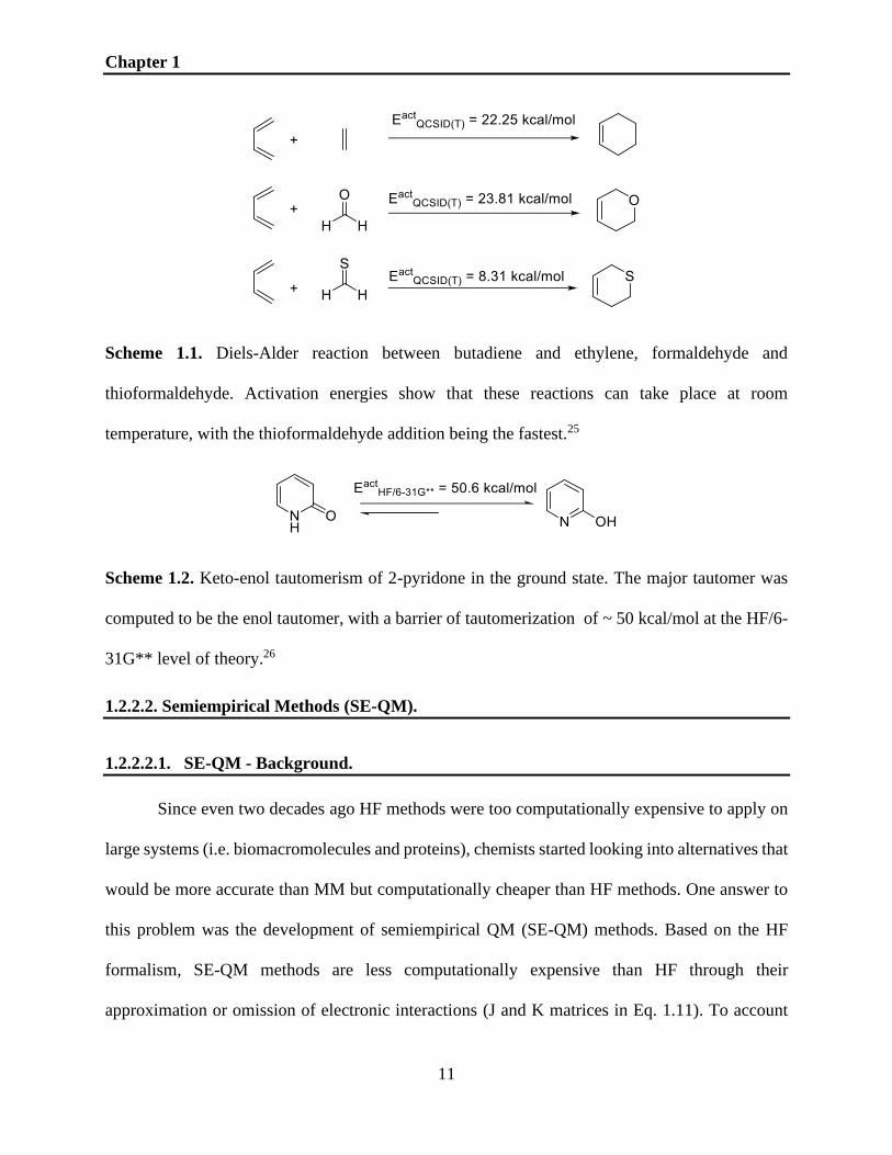
Chapter 1
11
Scheme 1.1. Diels-Alder reaction between butadiene and ethylene, formaldehyde and
thioformaldehyde. Activation energies show that these reactions can take place at room
temperature, with the thioformaldehyde addition being the fastest.25
Scheme 1.2. Keto-enol tautomerism of 2-pyridone in the ground state. The major tautomer was
computed to be the enol tautomer, with a barrier of tautomerization of ~ 50 kcal/mol at the HF/6-
31G** level of theory.26
1.2.2.2. Semiempirical Methods (SE-QM).
1.2.2.2.1. SE-QM - Background.
Since even two decades ago HF methods were too computationally expensive to apply on
large systems (i.e. biomacromolecules and proteins), chemists started looking into alternatives that
would be more accurate than MM but computationally cheaper than HF methods. One answer to
this problem was the development of semiempirical QM (SE-QM) methods. Based on the HF
formalism, SE-QM methods are less computationally expensive than HF through their
approximation or omission of electronic interactions (J and K matrices in Eq. 1.11). To account
Chapter 1
12
for the electronic interactions, SE-QM use empirical parameters that are fitted to reproduce
experimental data.27 Moreover, the most common SE-QM methodologies use specially optimized
Slater-type minimal basis set approximations to ensure fast and relatively reliable calculations.
Several SE-QM have been developed, such as AM1,28 PM3,29 PM6,30 and RM1,31 which have
been extensively used in conjunction with large systems (i.e. water clusters, nucleic acids,
proteins).24,32 Several important developments to SE-QM methods have been made to accurately
depict the non-covalent interactions found in biological systems, including dispersion, hydrogen-
bonding, and halogen-bonding corrections.24
1.2.2.2.2. SE-QM - Limitations.
Several limitations plague SE-QM methods, as they did in the case of the “parent” approach
(HF). First, as was the case with HF, correlation is generally not described. Moreover, when using
SE-QM methods on small organic molecules one must be careful, as qualitatively and
quantitatively wrong results will be obtained for molecules that are dissimilar from the molecules
used to parametrize the methods.24 Another limitation stems from the use of the minimal basis set,
which leads to the underestimation of intermolecular polarization and affects non-covalent
interactions.33 In addition to this, the majority of SE-QM methods only consider valence electrons.
1.2.2.2.3. SE-QM - Applications.
One of the most widely used SE-QM methods is PM6, which has been successfully used
in generating optimized protein structures and determining several protein properties, such as
secondary and tertiary structures. Moreover, PM6 has been used to model the formation of a
tetrahedral intermediate in chymotrypsin (Scheme 1.3).34

Chapter 1
13
Scheme 1.3. Formation of a tetrahedral intermediate in chymotrypsin.34 Distances for the transition
state (TS) are given in Ångstrom. New covalent bond between O-C in the tetrahedral intermediate
is shown in red. R and R’ can be any substituent. The TS was verified to contain only one negative
frequency.34
Another interesting application of SE-QM methods is the prediction of host-guest binding
affinities in supramolecular chemistry. In a study by Muddana and Gilson,35 the PM6-DH+ method
developed by Korth36 (DH+ represents dispersion and hydrogen bonding corrections to the PM6
method) was used to calculate the binding affinities of 29 guest complexes in conjunction with
cucurbit[7]uril. The authors found a strong correlation between computed and experimentally
determined binding free energies, showcasing the versatility of SE-QM methods.
1.2.2.3. Density Functional Theory (DFT).
1.2.2.3.1. DFT - Background.
While HF and SE-QM methods are useful in certain circumstances, there are times when
the system under scrutiny requires computing with a high degree of accuracy, such is the case for
predicting molecular properties of organic molecules, breaking/forming covalent bonds or
computation of stereoselectivities. For these purposes, density functional theory (DFT) was
developed in the 1960s by Kohn and Hohenberg and later by Kohn and Sham. DFT differs
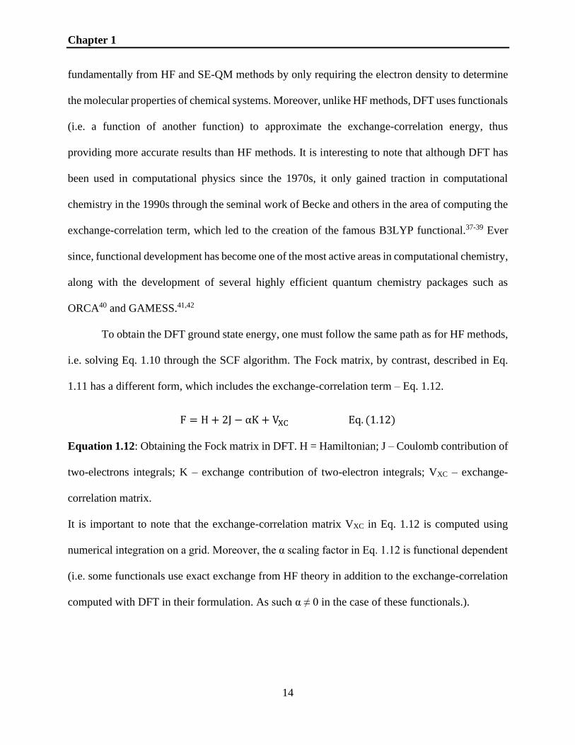
Chapter 1
14
fundamentally from HF and SE-QM methods by only requiring the electron density to determine
the molecular properties of chemical systems. Moreover, unlike HF methods, DFT uses functionals
(i.e. a function of another function) to approximate the exchange-correlation energy, thus
providing more accurate results than HF methods. It is interesting to note that although DFT has
been used in computational physics since the 1970s, it only gained traction in computational
chemistry in the 1990s through the seminal work of Becke and others in the area of computing the
exchange-correlation term, which led to the creation of the famous B3LYP functional.37-39 Ever
since, functional development has become one of the most active areas in computational chemistry,
along with the development of several highly efficient quantum chemistry packages such as
ORCA40 and GAMESS.41,42
To obtain the DFT ground state energy, one must follow the same path as for HF methods,
i.e. solving Eq. 1.10 through the SCF algorithm. The Fock matrix, by contrast, described in Eq.
1.11 has a different form, which includes the exchange-correlation term – Eq. 1.12.
F = H + 2J − αK + VXC Eq. (1.12)
Equation 1.12: Obtaining the Fock matrix in DFT. H = Hamiltonian; J – Coulomb contribution of
two-electrons integrals; K – exchange contribution of two-electron integrals; VXC – exchange-
correlation matrix.
It is important to note that the exchange-correlation matrix VXC in Eq. 1.12 is computed using
numerical integration on a grid. Moreover, the α scaling factor in Eq. 1.12 is functional dependent
(i.e. some functionals use exact exchange from HF theory in addition to the exchange-correlation
computed with DFT in their formulation. As such α ≠ 0 in the case of these functionals.).

Chapter 1
15
1.2.2.3.2. DFT - Limitations.
Although DFT methods account for the correlation term, they still suffer from the same
inability as HF methods to describe intermolecular interactions, especially vdW forces.43
Nevertheless, major advancements have been made in this area through the work of Grimme with
his DFT-Dn(n=1,2,3,4) schemes44 that allow a correct treatment of long-range interactions. Most
importantly, these schemes are easy to implement and very fast to compute, making them a must-
have for any DFT calculation. Grimme has also been the proponent of several low-cost composite
methods for the accurate description of large systems (i.e. biomacromolecules or proteins)
including the PBEh-3c and B97-3c methods.45,46 These methods use relatively small basis sets but
include corrections for basis set superposition error (BSSE) and long-range dispersion interactions,
which makes them highly appealing for biological systems.
Another major limitation of DFT is the self-interaction error (SIE). When describing the
correlation energy using an exchange-correlation functional, the interaction of an electron with
itself is taken into account. This behavior is wrong and is evident primarily in systems with
unpaired electrons. This leads to quantitively and qualitatively wrong results, as is the case for the
dissociation of carbocation radicals, which often give large errors when computing binding
energies.47 Moreover, due to the SIE, DFT encounters issues with describing some transition metal
complexes, including spin states and binding free energies.48
1.2.2.3.3. DFT - Applications.
As outlined above, DFT is highly useful for describing properties of organic molecules and
chemical phenomena such as breaking/forming of covalent bonds and computing
enantioselectivities. These will be discussed in depth in section 1.4 but we will highlight some
examples in this section as well. For instance, DFT (B3LYP/6-31+G** level of theory) has been

Chapter 1
16
successfully used to assign vibrational frequencies and normal modes of flavonoid derriobtusone
A using predicted and experimental IR and Raman spectra (Figure 1.3).49
Figure 1.3. Structure of derriobtusone A (left). Comparison between the experimental and
predicted Raman spectra (middle) and IR spectra (right) for derriobtusone A. Spectra taken from
reference 49.
In addition to molecular properties and vibrational spectra, DFT has been used to rationalize
numerous reaction mechanisms. Among the most interesting ones we mention the mechanism of
the first selenium organocatalyzed syn-dichlorination of alkenes.50 In the original paper, Cresswell
et al.50 proposed PhSeCl as the active catalyst. However, a DFT study by Fu et al.51 at the
B3LYP/6-311++G** level of theory showed that using PhSeCl as the catalyst leads to an
endergonic reaction (Figure 1.4), while using PhSeCl3 as the active catalyst led to a very favourable
exergonic reaction (Figure 1.5).

Chapter 1
17
Figure 1.4. Reaction mechanism in acetonitrile of the selenium organocatalyzed syn-
dichlorination of 2-pentene using PhSeCl as the active catalytic species. The reaction is endergonic
by ~ 17 kcal/mol. Figure reproduced from reference 51.
Figure 1.5. Reaction mechanism in acetonitrile of the selenium organocatalyzed syn-
dichlorination of 2-pentene using PhSeCl3 as the active catalytic species. The reaction is exergonic
by ~ 45 kcal/mol. Figure reproduced from reference 51.

Chapter 1
18
Fu et al. also showed that the rate-limiting step of the reaction has a barrier of only 13.9 kcal/mol
for PhSeCl3 (TS1-2, Figure 1.5), which agrees with the experimental data that the reaction happens
readily.
Beyond the ability of rationalizing reactions mechanisms, DFT has also been used to
develop new organocatalysts. In a study by Fleming et al.52 a highly active urea catalyst was
developed for addition reactions to epoxides (Scheme 1.4).
Scheme 1.4. Reaction scheme for the indole addition to styrene oxide in the presence of a urea
catalyst. Scheme reproduced from reference 52. Catalyst shown in blue.
This catalyst was selected based on structural optimization at the B3LYP/6-31G* level of theory
in the presence of the styrene oxide. The hydrogen-bonding interactions between the catalyst and
epoxide were deemed crucial for the catalyst reactivity (Figure 1.6).

Chapter 1
19
Figure 1.6. Hydrogen bonding interactions between the urea catalyst and styrene oxide. Key
interactions are shown with dashed red lines. Figure reproduced from reference 52.
1.2.3. Quantum Mechanics/Molecular Mechanics (QM/MM).
As outlined in the previous sections, MM methods are very useful at describing entire
proteins or large biomacromolecules, while QM methods are useful at describing organic
molecules with the occasional application to larger systems. However, in some cases, it is highly
desirable to combine the two methods – QM and MM – to study important aspects of chemistry,
such as stereoselective and/or regioselective protein catalysis. The main idea behind this hybrid
approach – QM/MM – is the treatment of a small number of atoms using highly accurate QM
methods (generally the ligand of interest and key amino acids in the active site of the protein) while
treating all the other atoms with MM methods. This approach allows the computation of long-
range electrostatic terms and steric effects that contribute to enzyme reactivity while accurately
describing the bond breaking/formation process between the ligand and active site residues.53 The
QM/MM approach has been used, for example, to propose a credible mechanism for the
regioselective chlorination of tryptophan (Trp) in the biosynthesis of pyrrolnitrin (Scheme 1.5), an
antifungal antibiotic, by the Trp-7-halogenase.54
Scheme 1.5. Transformation of Trp to pyrronitrin.

Chapter 1
20
The QM/MM study showed that two aminoacids, K49 and E346, played a major role in stabilizing
the intermediate products formed during the reaction between hypochlorous acid (HOCl) and Trp
(Scheme 1.6).
Scheme 1.6. Proposed regioselective mechanism from reference 54.
In addition to studying stereoselective protein catalysis, QM/MM methods have also been
used for docking. For example, a QM/MM algorithm developed by Chaskar et al.55 overcomes
some of the FF limitations described in section 1.2.1.4. (polarization effects and metal-bound
complexes). This algorithm was tested on three different sets that included zinc and iron
metalloproteins and compared to classical docking studies. As expected, compared to classical
docking, the QM/MM algorithm showed a significant improvement due to accounting for
polarization and correctly treating oxidation and spin states using QM.
While QM/MM methods are extremely valuable tools and provide accurate results when
used correctly, it must be emphasized that they too suffer from drawbacks, some more serious than
others. First, QM/MM calculations are computationally demanding, and as such extended
simulations on large systems can be performed routinely on standard desktop PCs only using SE-
QM methods for the QM region. If computational resources allow (i.e. access to supercomputers
and parallel computing), QM/MM calculations can employ either HF or DFT for the QM region.

Chapter 1
21
Second, QM/MM simulations are not “black box” calculations – significant work must be put into
generating a correct starting system. As is the case for any molecular dynamics simulation, several
important steps must be undertaken before the simulations can be run: the correct protonation state
must be assigned to all ionizable amino acids in the active site, MM parameters have to be
generated in case they are missing from the FF used in the simulations, and the number and
placement of water molecules near and around the active site must be carefully assessed.56 Third,
when performing a QM/MM calculation, a decision has to be made with regards to counter ions
and charge neutralization. Currently, there is no consensus as to whether to add counter ions to the
system to neutralize the charge due to charged buried groups.56 However, a popular approach is
that after deciding on a pH at which to run the simulation and assignment of protonation states, the
total charge of the system is kept as is, while others propose that the decision to add counter ions
should be made depending on the system at hand.57
1.2.4. Machine Learning (ML).
In the previous sections we have described how computational methods use the information
from nuclei and electrons to compute properties and rationalize various chemical principles. In
this section we will focus on methods that use chemical patterns, including complex combinations
of functional groups and patterns that govern molecular properties to describe and rationalize
various aspects of chemistry.58 Among these methods we will mainly focus on machine learning
(ML), a field of artificial intelligence that uses extensive training sets to gain knowledge from them
and use it for predicting properties of new data.
1.2.4.1. ML – Background.
ML has seen an impressive surge of interest in chemistry in the past decade due to several
factors: 1) increased computational power available even for a non-specialist user, 2) availability

Chapter 1
22
of open-source data sets necessary to create predictive models and 3) development of several easy-
to-use software packages and libraries used to create ML models. A recent review by Cova and
Pais58 explored the exponential growth of publications involving ML models in chemistry over a
10-year timeframe (2008-2018), and showed that the number of publications skyrocketed from a
few hundred in 2008 (counted from 1970 onward) to over 8000 in 2018. This significant increase
was prevalent in fields such as quantum, organic and medicinal chemistry, where ML methods
were used to improved existing methodologies and to aid in the design and synthesis of new
molecules.58 To better understand ML techniques and their applications, we will take a closer look
at the most popular models that have had widespread success in chemistry applications: artificial
neural networks (ANNs) and Random Forest (RF) models.
1.2.4.2. ML - Artificial Neural Networks.
Artificial neural networks (ANNs) are ML models that can fall under two categories. The
first category is that of supervised learning, meaning they require training data in order to learn
and infer the parameters of the function described by the ANN architecture. These parameters are
then used to describe novel data (or testing set). The second category is that of unsupervised
learning, meaning that the ANNs look for patterns in non-labeled input data. ANNs resemble a
biological neural network (Figure 1.7), with the basic unit being the artificial “neuron” connected
to other “neurons” through “synapses”. Neurons (or nodes) can be of three types: input nodes
(which takes numerical data presented as input), hidden nodes, and output nodes. The input data
is presented in the form of activation values i.e. each node has an input value made of a series of
numbers (often normalized in the [0,1] range) that describe molecules. As such, the ANN must
understand the molecular description (i.e. its simplified molecular-input line-entry system
(SMILES) classification),59 and molecular properties and convert them to usable numbers. It is

Chapter 1
23
important to mention that the higher the input number, the greater the activation. As can be seen
in Figure 1.7, the activation values are passed through the neural network by the means of hidden
nodes. The activation values are weighted before reaching the hidden nodes. Each hidden node
can receive several activation values, which it then sums up. However, before a meaningful output
can be delivered by the ANN, the information passing through the network must be translated by
a transfer function. This is done at each node that receives activation values by the means of
common transfer functions such as sigmoid or Gaussian. Depending on the task at hand, several
layers of neurons may be required to produce the required output. The first application of ANNs
in chemistry dates back to 1973, when Hiller et al.60 used an ANN to predict the bioactivity of 1,3-
dioxanes. Ever since, pharmaceutical companies and academic groups alike have used ANNs to
improve the drug discovery rate. For example, Jaen-Oltra et al.61 used ANNs on a series of 111
quinolones (molecules with antibacterial activity) in order to build a model that would predict the
minimum inhibitory concentration (MIC) of quinolones.
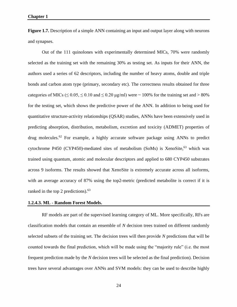
Chapter 1
24
Figure 1.7. Description of a simple ANN containing an input and output layer along with neurons
and synapses.
Out of the 111 quinolones with experimentally determined MICs, 70% were randomly
selected as the training set with the remaining 30% as testing set. As inputs for their ANN, the
authors used a series of 62 descriptors, including the number of heavy atoms, double and triple
bonds and carbon atom type (primary, secondary etc). The correctness results obtained for three
categories of MICs (≤ 0.05, ≤ 0.10 and ≤ 0.20 μg/ml) were ~ 100% for the training set and > 80%
for the testing set, which shows the predictive power of the ANN. In addition to being used for
quantitative structure-activity relationships (QSAR) studies, ANNs have been extensively used in
predicting absorption, distribution, metabolism, excretion and toxicity (ADMET) properties of
drug molecules.62 For example, a highly accurate software package using ANNs to predict
cytochrome P450 (CYP450)-mediated sites of metabolism (SoMs) is XenoSite,63 which was
trained using quantum, atomic and molecular descriptors and applied to 680 CYP450 substrates
across 9 isoforms. The results showed that XenoSite is extremely accurate across all isoforms,
with an average accuracy of 87% using the top2-metric (predicted metabolite is correct if it is
ranked in the top 2 predictions).63
1.2.4.3. ML - Random Forest Models.
RF models are part of the supervised learning category of ML. More specifically, RFs are
classification models that contain an ensemble of N decision trees trained on different randomly
selected subsets of the training set. The decision trees will then provide N predictions that will be
counted towards the final prediction, which will be made using the “majority rule” (i.e. the most
frequent prediction made by the N decision trees will be selected as the final prediction). Decision
trees have several advantages over ANNs and SVM models: they can be used to describe highly

Chapter 1
25
dimensional data, they can discard irrelevant descriptors, and can be interpreted easily by
chemists.64 As such, RF models have been highly sought after in the drug discovery field. For
example, an essential molecular lipophilicity descriptor used in drug discovery is the octanol/water
partition coefficient logP. A highly lipophilic molecule (logP > 5) will be poorly soluble, and as
such will have low bioavailability. In contrast, a lightly lipophilic molecule (logP < 2) will be
soluble and highly bioavailable.
Figure 1.8. Decision tree describing whether a drug candidate would be kept or discarded based
on its logP value.
During QSAR or virtual screening (VS) studies, a decision tree like the one in Figure 1.8
can be built and integrated into a larger RF model to determine whether a molecule would be
suitable for synthesis and testing. In addition to QSAR and VS studies, RF models have also been
used in docking to improve scoring functions. For example, Wang and Zhang65 developed a new
protein-ligand binding scoring function based on RF using a highly accurate training set containing
over 3000 experimentally-determined binding affinities and over 3000 computer-generated
decoys. Their RF model was built using 20 descriptors and exhibited a Pearson coefficient R =
0.73, which was shown to be superior to the best classical scoring function tested (R = 0.64).

Chapter 1
26
Moreover, as was the case with ANNs, RF models can be used to accurately predict SoMs.
Recently, a method developed by Finkelmann et al.66 used an RF model built with atomic
descriptors related to both the electronic and steric environments of atoms in molecules. The model
was tested on the XenoSite dataset and led to an average accuracy of 90.9% using the top2-metric.
1.2.4.4. ML – Limitations.
While ML models are generally robust and provide accurate results, they are not without
drawbacks. First, ML models are only as accurate as the data used for training them. While several
datasets (SoMs, protein-ligand binding affinities etc.) have recently been made available for QSAR
and VS studies, the data might not necessarily be uniform. For example, when it comes to SoM
determination, there are several assays that can be used to determine which CYP isoform is
responsible for substrate oxidation. Depending on the assay and conditions employed (which might
differ between laboratories) non-uniform data will be collected, which will ultimately impact the
ML models that predict SoMs.27 Second, a high-quality dataset must also be large enough for
training as well as highly diverse. If the dataset is small the model will be poorly predictive due to
overfitting of parameters. Moreover, if the dataset is not diverse enough, the RF model can only
be used to predict properties of similar molecules (similar to SE-QM methods discussed in section
1.2.2.2).27
1.3. Computational Tools in the Context of Medicinal Chemistry and Drug Discovery.
In the previous sections we have discussed the background of the most important
computational methods currently in use in chemistry and some applications and drawbacks of
each. In this section we will expand on the usage of these methods in drug discovery and
development, a field tightly entwined to medicinal chemistry. Moreover, we will highlight the

Chapter 1
27
requirements that medicinal chemists have when it comes to the application of these methods in
terms of usability and underlying methodologies.
1.3.1. Computer-Aided Drug Design (CADD).
It is well known that drug discovery is a highly tedious and expensive endeavour. Overall
it takes approximately 9 years on average to bring a drug to the market with a total development
cost of ~$2 billion.67,68 To shorten the required time to bring a drug to the market and to reduce
the associated costs, medicinal chemists have advocated for the introduction of computer-aided
drug design (CADD) techniques in the drug discovery pipeline. Indeed, it has been proposed that
using CADD tools in this process could lead to an overall cost reduction of 50%.69 However, to
streamline the usage of CADD tools in drug design, medicinal chemists require 1) user-friendly
software in a “black box” environment, 2) accurate and reliable software that is ideally contained
within one drug design platform and 3) simple and easy to read output that can be visualized if
necessary (i.e. protein-ligand interactions). These requirements are paramount because medicinal
chemists often have no expertise in computational chemistry. Moreover, to complement the
experimental tools that medicinal chemists have at their disposal and to ensure that the correct
computational tool is used in the drug discovery process, CADD methods have been divided into
two subcategories: structure-based drug design (SBDD) and ligand-based drug design (LBDD).
1.3.1.1. Structure-Based Drug Design (SBDD).
SBDD is a category of CADD that uses the 3D structure of a validated biological target
(enzyme or receptor) in order to develop high-affinity ligands or inhibitors.70 In this method, the
emphasis is put on the interactions between the target and ligand, including binding poses,
conformational preferences and reaction mechanisms.27 Generally, the target structure is

Chapter 1
28
determined through either NMR, X-ray crystallography or homology modelling. Amongst the
most important techniques in SBDD are molecular docking, VS and MD simulations.
1.3.1.1.1. SBDD - Molecular Docking.
Molecular docking is an essential tool in the repertoire of medicinal chemists. In short,
docking is a method that explores the behaviour of a ligand inside the active site of a target. Often
the underlying theory behind docking is MM-based, although rule-based docking methods exist as
well. The docking procedure consists of two distinct steps: conformational search and scoring.
To perform the conformational search, several algorithms can be employed. For example,
the docking program FITTED71
uses a highly efficient genetic algorithm to find the best ligand poses
inside the active site of the target. If during the conformational search the parameters of the ligand
and protein (bond lengths, angles, and torsions) do not change, the docking technique is called
rigid-body docking. This technique is a direct consequence of the “lock and key” mechanism of
enzyme-ligand interactions, which assumes that only the right ligand will fit inside the active site
of a target enzyme. It has been shown that rigid body docking has a far greater accuracy if the
crystal structure was co-crystallized with a ligand rather than in its apo structure.72 If the
parameters change during the docking process to account for variations in the ligand and protein
conformations, the technique is called flexible docking. Flexible docking was developed as a
consequence of the “induced-fit” theory introduced by Koshland,73 where an enzyme can change
conformations to accommodate an incoming ligand. It is worth noting that flexible docking is more
computationally demanding than rigid body docking due to the sampling of different side chain
and/or backbone and ligand conformations.
When the conformational search is complete, the binding poses are scored to determine the
most likely conformation of the ligand inside the active site. While scoring functions differ

Chapter 1
29
between docking programs, they generally involve MM-based energy terms such as electrostatics
and vdW interactions between ligands and target along with more complex terms.
Over time several docking programs have been developed – AutoDock,74 Glide,75 GOLD,76
FITTED – and successfully used in the drug discovery process. Importantly, these docking programs
all have somewhat easy-to-use interfaces that allow medicinal chemists to undertake their own
docking studies. Moreover, at the end of a docking run, it is possible to visualize the preferred
binding poses inside the active site of the enzyme target. This visualization is important because it
gives medicinal chemists the opportunity to assess the structural integrity of the protein-ligand
complex, as well as to visually assess if the desired interactions between enzyme and ligand are
fulfilled. In addition, a medicinal chemist could use their chemical intuition to elicit changes in the
ligand to improve the binding affinity and then dock the improved compound and compare to the
original to test their hypothesis. Success stories that involved molecular docking include the in
silico development of Zanamivir (influenza drug),77 the first neuraminidase inhibitor to be
commercially developed, and the rationalization of nelfinavir HIV-1 protease resistance, which
lead to the development of more potent analogues.78
1.3.1.1.2. SBDD - Virtual Screening.
At the onset of any drug development project a decision must be made with respect to
which type of compounds should be pursued. Knowledge and information about the biological
target are paramount, as well as that of key interactions in the active site of the target that should
be fulfilled by a possible drug. Therefore, the question is: what is the starting point for developing
a new drug?
Thankfully, sustained efforts by several pharmaceutical companies and academic groups
have led to the creation of large commercially available small-molecule libraries that cover a large

Chapter 1
30
area of the available chemical space. Databases such as ZINC79 and Chemspace80 have proven to
be invaluable when it comes to providing a suitable starting point for a drug design project. These
databases can then be screened to obtain a series of drug-like molecules that can be docked into
the target enzyme to assess their suitability as ligands or inhibitors or used in LBDD methods. The
top compounds can then be selected as lead compounds, synthesized, or purchased and biologically
tested. As such, obtaining a hit compound can be done exclusively in silico and the first stage of
the drug development process (i.e. hit discovery) can be resolved in a matter of days or weeks.
This entire approach is known as virtual screening. To enable medicinal chemists to undertake
their own VS studies without proficiency in software development or command line environments,
drug discovery platforms such as FORECASTER81 have been developed. FORECASTER was
developed by chemists for chemists, and it provides inexperienced users with a graphics user
interface (GUI) that automates the process of running a VS study without the need to know the
underlying theories. VS has become standard for drug design and has led to several success stories,
such as finding novel inhibitors for DNA methyltransferase (involved in cancer)82 and a potent
drug candidate against tyrosine phosphorylation regulated kinase 1A (involved in Down
Syndrome).83
1.3.1.1.3. SBDD - MD Simulations.
As described in section 1.3.1.1.1, docking is an essential tool in drug discovery. However,
docking only provides a static picture of ligand-enzyme interactions. At times, it is desirable to
observe the effects of these ligand-enzyme interactions over time to better understand the processes
that take place while the enzyme is performing its biological function. One method of tracking
these interactions and changes in enzyme structure is through MM-based MD simulations.
Through the usage of modern computing facilities, simulations of more than 100000 atoms are

Chapter 1
31
now routine84 and the timescales on which MD simulations can be run range from picoseconds to
milliseconds.17 Moreover, depending on the level of detail required for the simulations, MD can
be performed at either the atomistic level (each atom is represented individually) or using coarse-
grained representations. For example, if one is interested in observing bond breaking/formation
during protein catalysis, it would be advisable to use MD simulations at the atomistic level. This
approach is, however, computationally demanding, and it should only be employed if the protein
of interest is relatively small and the timescale of simulation relatively short. On the other hand, if
one is interested in protein folding, which occurs on a long timescale (micro to milliseconds), a
coarse-grained MD simulation can be undertaken. In the coarse-grained representation, entire
functional groups or amino acid residues are represented by “beads” in order to speed up the
simulations and to reduce the computational cost.85
To perform an MD simulation, several steps must be undertaken prior to starting the
simulation. First, a good initial structure for the enzyme is required. This structure can either be
taken from X-ray crystallography, NMR, homology modeling, or cryogenic electron microscopy
(Cryo-EM). Then, hydrogen atoms must be added to the crystal structure to prepare it for the
simulation and the correct protonation state must be assigned to the ionizable amino acids. Once
the structure is ready for simulation, the overall enzyme charge may be neutralized through the
addition of counter ions, followed by the placement of the enzyme in a box of solvent (water,
methanol etc.) to obtain a realistic solvent effect. While this adds complexity to the system, it
allows a more accurate description of entropic effects (i.e. hydrophobic effects).84 Next, as
described in section 1.2.3, a decision has to be made whether charge equilibration should be
performed or not. Once all these steps have been fulfilled, the simulation can be run. The steps
described above are non-trivial and are in fact largely inaccessible to medicinal chemists.84 As

Chapter 1
32
such, developers of MD software packages such as NAMD86 have spent considerable time in
providing a comprehensive and user-friendly GUI that automates these steps, hiding the underlying
theory for easier use. These developments have led to several successes in the application of MD
simulations to drug discovery, such as identifying cryptic binding sites.87
In one example, a novel trench-like binding site was identified for HIV-1 integrase, which
led to the discovery of raltegravir, the first FDA-approved drug for this enzyme.88 Another
application of MD in drug discovery is the accurate computation of ligand binding energies. For
instance, a series of azoles were optimized as potent anti-HIV agents starting from inactive
scaffolds through free energy perturbation calculations.89 Based on these calculations, two
compounds were selected and tested in vitro where they exhibited high nM activity (300-800 nM
range). To improve their potency, they were subsequently modified based on the ligand binding
energy calculations to improved compounds with low nM (10-20 nM range) activity.
1.3.1.2. Ligand-Based Drug Design (LBDD).
In contrast to SBDD, LBDD is used when 3D information about the biological target of
interest is unavailable. Active compounds such as drugs must be developed indirectly by carefully
studying the known substrates and/or inhibitors of a target.90 The most popular approaches in
LBDD involve QSAR studies and pharmacophore modeling, which will be discussed below.
1.3.1.2.1. LBDD – QSAR.
When compounds (substrates or inhibitors) are known for a biological target, it is desirable
to map the relevant features (key physicochemical characteristics) to understand their activity and
the relation between their structure and activity (structure-activity relationship). Then, analogues
with improved potency and/or drug-likeness can be designed while maintaining the core features
that afford activity. This is the underlying theory behind QSAR, a computational method used for

Chapter 1
33
quantifying the relationship between the structural features of a molecule and its biological
activity.90 To maximize the biological activity of subsequent analogues of a compound of interest,
a mathematical model is built using molecular descriptors of these compounds (such as logP, pKa,
and molecular weight) and the stability and robustness of the model is verified against biological
activity. The paramount aspect of QSAR is the selection of descriptors - only those descriptors that
affect biological activity should be chosen. This can be done using several statistical methods, such
as linear regression, principal component analysis or partial least square analysis.90 Some QSAR
models (comparative molecular field analysis - CoMFA91 and comparative molecular similarity
indices - CoMSIA92) use 3D descriptors to build models that relate to biological activity. The
advantage of applying such descriptors is that they use both steric and electrostatic molecular
features to relate to biological activity. However, these 3D descriptors are highly dependent on the
conformation of the compound of interest. Generally, such compounds are optimized using MM
or QM techniques to obtain the lowest-energy conformation, which is then assumed to be the
biologically active one. This assumption might not always hold, and as such a major pitfall of 3D
QSAR techniques is building erroneous models based on the wrong active conformer.
Nonetheless, 3D QSAR methods - CoMFA and CoMSIA - have been applied successfully to
various aspects of drug design, chiefly the optimization of mercaptobenzensulfonamides as HIV-
1 integrase inhibitors93 and the design of 1,4-dihydropyridines as calcium channel blockers.94
1.3.1.2.2. LBDD - Pharmacophore Modeling.
While pharmacophore modeling has generated interest in drug discovery only in the past
few decades, the concept of a pharmacophore was introduced as early as the beginning of the 20th
century.95 Across the decades, medicinal chemists have offered different definitions for a
pharmacophore, including a highly popular one given by Schueler96 in 1961: “a molecular

Chapter 1
34
framework that carries (phoros) the essential features responsible for a drug’s (pharmacon)
biological activity.” To unify the existing definitions, the International Union of Pure and Applied
Chemistry (IUPAC) provided an updated description of a pharmacophore in 1997: “a
pharmacophore is the ensemble of steric and electronic features that is necessary to ensure the
optimal supramolecular interactions with a specific biological target structure and to trigger (or to
block) its biological response”.97 A pharmacophore is comprised of structural features such as
hydrogen-bond donors/acceptors and hydrophobic, halogen or aromatic moieties that contribute to
a molecule’s biological activity (Figure 1.9).
Figure 1.9. Structure of Clobazam13 (left) and its pharmacophore (right). Red – halogen moiety;
blue – aromatic moiety; green – hydrogen bond acceptor; purple – hydrophobic moiety.
In drug discovery, a pharmacophore model is usually generated on a training set made of
compounds that are known to be active on a specific target. The molecules have their
conformations sampled through various algorithms, followed by molecular alignment and
assembly of their pharmacophore features.98 Sampling algorithms have to account for ligand
flexibility, which is one of the main challenges of pharmacophore modeling. This can be achieved
by pre-generating multiple conformations for each ligand and saving them in a database, or
computing them on-the-fly during the generation of the pharmacophore model. Regardless of
method, the sampling of the conformational space must ensure that all biologically-relevant
conformations have been considered.98

Chapter 1
35
Apart from ligand flexibility, the alignment of various ligands represents a different
challenge. Molecular alignment can be carried out in two different ways: atom-by-atom mapping
and mapping based on molecular features. For structures with similar atomic environments, atom-
by-atom mapping represents a good choice. However, for highly dissimilar ligands, mapping based
on molecular features is more advantageous because it precludes the usage of pre-defined anchor
points necessary for atom-by-atom mapping.98 Another challenge of pharmacophore modeling is
represented by the choice of training set; it has been shown that depending on the training set,
completely different pharmacophore models can be generated for the same target using the same
software.99-101
Despite these challenges, pharmacophore modeling has seen widespread use in the drug
discovery community. A study by Ren et al.102 used pharmacophore modeling in conjunction with
VS to find potent in vitro and in vivo inhibitors of transforming growth factor-β Type I receptor.
In a different example, pharmacophore modeling combined with docking led to the discovery of
potent compounds against human leukotriene A4 hydrolase and the human nonpancreatic secretory
phospholipase A2.103 In another study, successful virtual activity profiling was achieved on a set
of 100 antiviral compounds and several antiviral targets using a novel pharmacophore-based
parallel screening approach.104
1.4. Computational Tools in the Context of Organic Chemistry.
In the previous section we described how computational tools are used to improve the drug
discovery process and the overall molecular discovery rate. Nevertheless, these tools have far-
reaching implications in many other fields, such as organic chemistry and more specifically
organic synthesis. For example, ML methods have been used with some success in retrosynthetic
analyses and synthesis design.105-107 Nonetheless, these methods have several drawbacks. One

Chapter 1
36
drawback is that it does not consider stereochemistry changes during reactions, and it also provides
reaction pathways that are either too long or unfeasible.108 These current drawbacks preclude the
implementation of these tools in wet labs, but do provide an important stepping stone in the overall
endeavour of using computational tools in organic synthesis. Moreover, the area of reaction
prediction and design is still under active development and will likely yield successful
methodologies for experimentalists to use. Apart from the usage of ML methods for synthesis
design, other computational tools have been widely used in organic synthesis to rationalize
reaction mechanisms, chemical reactivity and stereoselectivities of various organic and metal-
based catalysts. The usage of these tools, along with relevant examples and success stories will be
discussed below.
1.4.1. Reaction Mechanisms.
The breaking and formation of bonds occurs on an attosecond timescale.109 Experimental
measurements of such phenomena require incredibly complex equipment, and is beyond the means
of most organic chemists. As such, computational chemistry has taken over the role of explaining
how chemical bonds form and break. Among the most widely used tools to explore reaction
mechanisms is DFT, because of its low computational cost in comparison to post-HF methods and
its relatively high accuracy. DFT is particularly well suited in describing the ground state
geometries of reactants and products, as well as exploring the reaction PES, locating TS structures,
and predicting side products. Increasingly, experimental chemists have collaborated with
computational chemists to rationalize experimental observations. Furthermore, due to significant
advancements in the development of user-friendly, highly efficient and accurate QM packages,
experimental chemists have slowly started running their own DFT studies.110

Chapter 1
37
To understand the necessity of DFT in elucidating reaction mechanisms, we will first refer
to the famous example mentioned in section 1.1: the Sharpless asymmetric dihydroxylation.4 To
understand how important DFT was in this case, we will take a closer look at the possible reaction
mechanisms proposed before theoretical studies were conducted, and how DFT was used to
differentiate between them. The Sharpless asymmetric dihydroxylation of alkenes (Scheme 1.7)
proceeds through an osmium-based catalyst and leads to the formation of chiral diols. This reaction
is of exceptionally high value in organic synthesis because it allows the introduction of chirality
in non-chiral compounds. Since its development, the Sharpless asymmetric dihydroxylation has
been extensively used in the total synthesis of natural products.111
Scheme 1.7. Sharpless asymmetric dihydroxylation of alkenes.
When the reaction was first described, Sharpless proposed that the mechanism went through a
[2+2] cycloaddition step that led to the formation of a 4-membered ring osmaoxetane (Scheme
1.8a), which would undergo ring expansion to convert to a 5-membered ring TS.112 Later, Corey
proposed that the mechanism actually proceeded through a [3+2] cycloaddition step that led to the
direct formation of a 5-membered ring TS without proceeding through an osmaoxetane
intermediate (Scheme 1.8b).113 These proposals sparked a decade-long debate between Corey and
Sharpless, with both producing experimental evidence for their respective mechanisms.
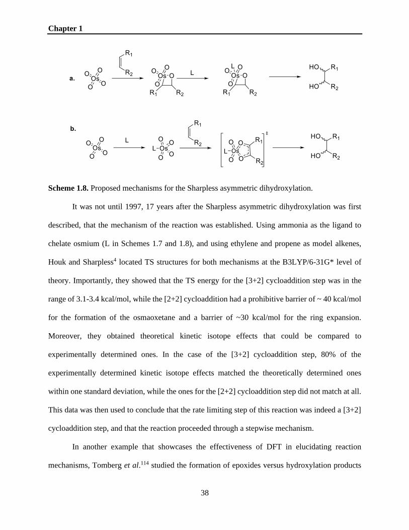
Chapter 1
38
Scheme 1.8. Proposed mechanisms for the Sharpless asymmetric dihydroxylation.
It was not until 1997, 17 years after the Sharpless asymmetric dihydroxylation was first
described, that the mechanism of the reaction was established. Using ammonia as the ligand to
chelate osmium (L in Schemes 1.7 and 1.8), and using ethylene and propene as model alkenes,
Houk and Sharpless4 located TS structures for both mechanisms at the B3LYP/6-31G* level of
theory. Importantly, they showed that the TS energy for the [3+2] cycloaddition step was in the
range of 3.1-3.4 kcal/mol, while the [2+2] cycloaddition had a prohibitive barrier of ~ 40 kcal/mol
for the formation of the osmaoxetane and a barrier of ~30 kcal/mol for the ring expansion.
Moreover, they obtained theoretical kinetic isotope effects that could be compared to
experimentally determined ones. In the case of the [3+2] cycloaddition step, 80% of the
experimentally determined kinetic isotope effects matched the theoretically determined ones
within one standard deviation, while the ones for the [2+2] cycloaddition step did not match at all.
This data was then used to conclude that the rate limiting step of this reaction was indeed a [3+2]
cycloaddition step, and that the reaction proceeded through a stepwise mechanism.
In another example that showcases the effectiveness of DFT in elucidating reaction
mechanisms, Tomberg et al.114 studied the formation of epoxides versus hydroxylation products

Chapter 1
39
in CYP450-mediated aromatic oxidations using the PBE0 functional and a custom built basis set.
This oxidation takes place through a radical mechanism. Using a simplified heme model along
with bromobenzene and phenol as model substrates (Scheme 1.9a), Tomberg et al. showed that
the nature of the intermediate (radical or cationic) played a major role in the resulting product
(Scheme 1.9b). Moreover, the authors were able to show that the spin density during the reaction
resides primarily on the iron if the resulting product was a hydroxide, while residing primarily on
the aromatic ring if the product was an epoxide. The elucidation of this mechanism is of high
importance in transition-metal catalysis, as well as in enzyme catalysis, where CYP450 have been
often used.

Chapter 1
40
Scheme 1.9. a) Simplified heme model used as reactive species in the reaction mechanism, along
with bromobenzene and phenol used as model substrates for the reaction. b) Reaction mechanisms
that lead to the formation of either epoxide or hydroxide.114
1.4.2. Chemical Reactivity.
The effectiveness of DFT studies is not only limited to the study of reaction mechanisms.
In fact, a whole new field of study built around DFT has emerged in the past few decades –
conceptual DFT (cDFT). cDFT has been successfully used in providing the theoretical basis of
qualitative chemical concepts, such as hardness, softness, electronegativity, chemical potential,
electrophilicity, and nucleophilicity.115 For example, the chemical potential μ of a molecule
represents the tendency of electrons to escape from a system in a state of equilibrium.116 Within
the DFT framework, μ can be computed as the sum of the energy of the lowest unoccupied
molecular orbital (LUMO) and highest occupied molecular orbital (HOMO) (Eq. 1.14).115 In
another example, to explain why acid-base reactions proceed in a set direction, Pearson introduced
the concept of “hardness” and “softness”, as well as the hard-soft acid-base (HSAB) theory.117 The
HSAB theory states that a hard nucleophile will preferentially react with a hard electrophile, while
a soft nucleophile will preferentially react with a soft electrophile. Within the framework of DFT,
the chemical hardness can be expressed as the difference between the energies of the LUMO and
the HOMO, while the softness is just the inverse of hardness (Eqs. 1.15-1.16).
μ =1
2 × (εLUMO + εHOMO) Eq. (1.14)
η =1
2 × (εLUMO − εHOMO) Eq. (1.15)
S =1
2η Eq. (1.16)

Chapter 1
41
Equations 1.14-1.16. Description of the global parameters chemical potential, hardness, and
softness.
The softness of a molecule relates to its polarizability, with a larger molecule being softer, thus
more polarizable. Once hardness and chemical potential were introduced as concepts, Parr et al.118
developed an electrophilicity index ω that makes use of them (Eq. 1.17).
ω =μ2
2η Eq. (1.17)
Equation 1.17. Description of the global electrophilicity ω.
This index is an excellent description of the energy stabilization obtained when the molecule
receives an additional electronic charge from the environment.115 Importantly, these indices only
provide information about molecular reactivity and stability. However, sometimes it is useful to
determine exactly which atom(s) within a molecule will react. To this end, local atomic reactivity
indices (LARIs) have been developed to account for the reactivity of individual atoms.
Among these, the most important are the Fukui functions.119 Based on Kenichi Fukui’s
seminal work on the role of the HOMO and LUMO orbitals in chemical reactions,120 the Fukui
functions (or coefficients – FC) relate the atomic electronic density in the HOMO and LUMO
orbitals to the propensity of an individual atom to undergo nucleophilic (f+), electrophilic (f-) or
radical attack (f0) (Eq.1.18-1.20).115
f+ = ρLUMO Eq. (1.18)
f− = ρHOMO Eq. (1.19)
f0 = 1
2 × (ρHOMO + ρLUMO) Eq. (1.20)
Equations 1.18-1.20. Description of the Fukui functions for nucleophilic, electrophilic, and
radical attacks.

Chapter 1
42
The Fukui functions have been applied extensively within the cDFT framework to explain local
atomic reactivity patterns. For example, the reactivity of lignin precursors p-coumarol, coniferol
and sinapol (Figure 1.10) was investigated in order to explain the formation of lignin, an aromatic
polymer present in the walls of wood cells.121
Figure 1.10. Structures of p-coumarol, coniferol and sinapol.
Since the formation of lignin involves a radical mechanism, the f0 values were computed and it
was shown that for p-coumarol and sinapol the β-carbon is the most reactive site, while for
coniferol the most reactive site is in the carbon-oxygen bond region of the hydroxyl group attached
to the γ carbon. In another example, Mendez and Gazquez122 looked at the reactivity of three
enolates: cyclohexanone, phenacyl and butyrolactone (Figure 1.11) using Fukui functions and the
HSAB theory.
Figure 1.11. Structures of the enolate ions of cyclohexanone, phenacyl and butyrolactone.
To understand the difference in reactivity between the different reactive sites, Mendez and
Gazquez computed the f- values for the three enolates. These values showed that the highest values

Chapter 1
43
for the electrophilic Fukui function resided on the carbonyl oxygen atom in all three cases,
followed by the enolate carbon. Moreover, they showed that depending on the substituents on the
enolate, the reactivity order can shift between the enolate carbon and carbonyl oxygen, effectively
changing the reactive site. This can occur if the reagent and solvent is kept constant. However,
changing the solvent can lead to a change in reactivity in the same enolate, which is supported by
experimental evidence.122 Overall, these examples serve as a validation of the usage of cDFT in
organic chemistry, and as proof of the ability of cDFT to aid chemists in their understanding of
chemical reactivity.
1.4.3. Catalyst Design, Screening and Enantioselectivity Computations.
Apart from rationalizing reaction mechanisms and chemical principles, computational
tools can also be used to design new molecules or new reactions. For example, of high interest in
organic chemistry are chiral molecules. To synthesize such molecules one could use biocatalysis
or a chiral pool; however, these methods have numerous drawbacks, such as the relative stability
and specificity of biocatalysts and the reduced number of chiral molecules available in the chiral
pool.18 An alternative to these methods is asymmetric synthesis, which allows one to synthesize
chiral molecules in high yield and purity. To allow for efficient asymmetric syntheses, cheap,
green, selective catalysts must be employed. Most commonly used catalysts in asymmetric
syntheses are metal based, which suffer from poor availability, high cost, and relative toxicity. To
avoid the usage of metals in catalysis, one can explore the organic catalysts for the required
chemical transformations. However, these catalysts must be designed and synthesized, a tedious
process if done only experimentally. Thus, screening and designing new catalysts computationally
has started gaining traction in the organic chemistry field.

Chapter 1
44
To enable the design of selective catalysts, one must first have an accurate method to
compute the stereoselectivity of the catalysts. To this end, several methodologies for designing
catalysts and computing stereoselectivities have been developed, including MM,123,124 QM,125-127
and QM/MM128 techniques. For example, Du et al.126 used DFT to predict the reactivity of
supported metal oxide for the selective catalytic reduction of nitrogen oxides with ammonia. In
their study, they used several DFT descriptors – LUMO, hydrogenation and HOMO energies – to
establish the oxidizing ability and acidity of potential oxide catalysts. In their search they separated
the potential catalysts in three categories: active components, promoters, and inactive
components/support. Those catalysts that exhibited strongly negative hydrogenation energies
(high oxidizing ability), combined with low LUMO energies (high acidity) and high HOMO
energies (possibility for reoxidation) were the active components of the reaction. These were
experimentally tested and found to correlate accurately with the theoretical study, providing an
excellent example about the usage of DFT in obtaining new catalysts.
However, while DFT has been used in catalyst screening and design, it suffers from several
drawbacks. First, the computation times of optimizing ground state geometries, finding TS
structures, and computing enantioselectivities might be prohibitive for organic chemists, especially
when libraries of potential catalysts must be screened. Second, it has been shown that popular
integration grids used for computing the exchange-correlation energy provide quantitatively wrong
results for computed stereoselectivities due to their lack of rotational invariance.129 Thus, due to
these drawbacks and to ensure a fast, efficient, and accurate screening of libraries of potential
catalysts, several academic groups have been working on providing user-friendly computational
platforms that use MM methods. Among the most comprehensive platforms are VIRTUAL
CHEMIST18
and CatVS.130

Chapter 1
45
VIRTUAL CHEMIST, developed in the Moitessier research group at McGill University, is a
state-of-the-art computational platform that allows an organic synthesis experiment to be simulated
from start to finish. Specifically designed for asymmetric synthesis, the platform was validated on
four different types of experiments: one-by-one design, library screening, hit optimization and
substrate scope evaluation. The platform was designed with the necessities of organic chemists in
mind and includes modular workflows that allows experimentalists to create their own experiments
through a few clicks. Most importantly, the underlying methodologies are hidden from the user
and using the platform does not require any computational expertise. When the platform was
developed, three main aspects were given special consideration: 1) preparation of libraries of
catalysts, 2) predicting stereoselectivities, and 3) evaluating catalytic activity.
The most important program in the VIRTUAL CHEMIST platform is the Asymmetric Catalyst
Evaluation (ACE)123 package. Based on the MM3 FF, ACE uses the Hammond-Leffler postulate
(Figure 12 top) to construct the TS as linear combination of reactants and products. The forming
bonds are considered as a combination of covalent bonds, present in the products, and non-covalent
interactions present in the reactants (Eq. 1.21).
ETS = (1 − λ)ER + λEP Eq. (1.21)
Equation 1.21. Description of the linear combination of reactants and products used by ACE to
construct the TS.
To ensure that the TSs are properly described, a Lamarckian genetic algorithm to optimize
and perform an exhaustive conformational space search of TS templates was implemented. After
the TSs for a given reaction have been optimized, ACE computes the stereoselectivities of a given
catalyst (in either vacuum or solvent) using the Curtin-Hammett principle (Figure 1.12 bottom).
Although ACE uses an MM-based FF for the conformational search, TS optimization and

Chapter 1
46
stereoselectivity computation, the accuracy of the program is within 1 kcal/mol when compared to
experimentally determined stereoselectivities (tested on 350 reactions from 7 reaction classes).18
The accuracy and ease-of-use makes the overall platform highly attractive for organic chemists.

Chapter 1
47
Figure 1.12. Top: Hammond-Leffler postulate: the TS resembles the reactants (A) if it is an early
TS and the products (B) if it is a late TS. The step λ controls whether the TS is late or early in the
ACE computations. Bottom: Schematic depiction of the Curtin-Hammet principle.
Stereoselectivity of a catalyst can be computed by converting the difference in energy between
TS1 and TS2 (i.e. ∆∆G‡) to an enantiomeric excess (%ee) ratio.
The underlying theory, auxiliary programs, drawbacks and extensive testing and validation of
VIRTUAL CHEMIST will be discussed in greater detail in Chapter 5.
Another important computational platform in the field of asymmetric synthesis is CatVS,
developed by Rosales et al.130 This platform is based on the quantum guided molecular mechanics
method (Q2MM),131 which allows the development of transition state force fields (TSFFs)132 using
QM data obtained for small model systems of a reaction’s TS. This methodology has been
validated on several reactions, such as metal-catalyzed oxidations and hydrogenations, P450
oxidations, and stereoselective additions to aldehydes.130 To explore the conformational space of
the possible TSs, CatVS uses the Monte Carlo routines available in Macromodel,133 while the
computation of stereoselectivities is done using Boltzmann-averaging of the energies of the
conformations that lead to a specific stereoisomer. To explore the applicability of CatVS to a
reaction of chemical interest, a library of ligands was screened for the Rh-catalyzed asymmetric
hydrogenation of enamides on two substrates (Scheme 1.10).

Chapter 1
48
Scheme 1.10. Overall scheme for the Rh-catalyzed asymmetric hydrogenation of enamides
(left).130 Substrate with a conjugated α-substituent (middle) and substrate with a non-conjugated
α-substituent (right).
To differentiate between screened ligands (L in Scheme 1.10), Rosales et al. set a threshold
of 96% for the enantiomeric excess. In the case of the substrate with a conjugated α-substituent,
CatVS was able to identify four correct ligands and one false positive. In the case of the substrate
with a non-conjugated α-substituent, CatVS found two highly selective ligands and failed to
identify one false negative. Despite these successes, CatVS presents drawbacks, such as the
inability to consider highly flexible or highly charged TSs, as well as the inability to model solvent
effects. Nonetheless, if the TSs of the reaction of interest are rigid and experimental data available
to compare to predictions, CatVS can be highly useful. Moreover, the VS study presented above
was performed on a standard PC in less than 12h per ligand, which makes it highly attractive to
organic chemists due to low computational requirements and fast turnover rate.
1.5. Conclusions.
In this chapter, we presented several computational tools and methodologies, each with
their associated background, limitations, and applications. Among the most interesting tools are
MM, QM, and ML methods, which have seen widespread use in various fields of chemistry. Most
importantly, we described the usage of these methods in the context of drug discovery/medicinal
chemistry and organic chemistry research.
Within drug discovery, computational tools are of extreme importance due to their ability
to shorten the time a drug requires to reach clinical trials, and to potentially reduce the failure rate
(reduced toxicity). Using computational tools in the drug discovery pipeline enables researchers
to test hypotheses much faster than they would experimentally (for example changing various

Chapter 1
49
functional groups on drug candidates and observing the interactions with a biological target
through docking or MD simulations), and allows them to obtain a hit compound in mere days or
weeks. This compound can then be tested for toxicity in silico. For example, computational tools
to assess the potential SoMs can be used to verify whether the lead compound could be metabolized
into harmful reactive metabolites. If this is the case, in silico structural changes can be made to the
compound to remove the possibility of reactive metabolite formation even before attempting
synthesis. This process ensures that only promising molecules are synthesized, which contributes
to a lower cost of the overall drug discovery process.
Within organic chemistry, computational tools can be used to rationalize reaction
mechanisms and chemical reactivity, but also to design new molecules and reactions. Throughout
the years, reaction mechanisms for highly synthetically relevant reactions, such as the Sharpless
asymmetric dihydroxylation and P450-mediated oxidation of aromatic compounds, have been
explained. Moreover, significant advancements in understanding chemical reactivity have been
made through the application of cDFT to chemical principles such as hardness, softness, chemical
potential, and electrophilicity. These examples showcase the power and utility of computational
tools when applied to problems of organic chemistry. In addition to this, we described the ability
to design and screen numerous catalysts in silico in a matter of days with user-friendly
computational platforms. These platforms are designed especially for experimentalists to allow
their manipulation with limited computational expertise. Most importantly, these tools allow
organic chemists to design and perform experiments in silico and to make any necessary
adjustments and changes to their hypotheses and reagents. Indeed, these tools enable scientists to
effectively remove tedious aspects of experimental chemistry and to focus on high-level problem
solving and experimental design.

Chapter 1
50
1.6.Thesis Objectives.
This thesis develops computational tools and protocols to improve the molecular discovery
rate in organic and medicinal chemistry. Overall, the thesis will address the advancements we have
made in this field, by considering three separate but interconnected examples. Chapters 2 and 3
will discuss the development of a computational protocol to accurately model the conformational
preferences of clinically-relevant nucleosides (historically used as drugs against diseases such as
HIV, cancer and herpes), and thereby enable the design and synthesis of those nucleosides with
desirable properties. Chapter 4 will present integration of QM, docking, and ML methods for
CYP450 inhibition prediction in the drug discovery pipeline, while Chapter 5 will focus on
improving the current tedious, costly process of developing asymmetric catalysts by delivering a
computational platform that has been experimentally validated by organic chemists for catalyst
discovery.

Chapter 2
51
Chapter 2 – Accurately Modeling the Conformational Preferences
of Nucleosides – Methodology
Preface.
Existing computational methods are useful in enabling the synthesis of compounds with
highly desirable properties, yet in some cases these methods need to be developed for special
classes of molecules. This is the case of nucleosides, which have historically been used as drugs
against diseases like cancer and HIV. Nucleosides are notorious for their modeling difficulty
because their conformations are highly sensitive to solvent and intrinsic stereoelectronic effects.
Since they owe their activity to their conformation, the ability to predict these conformations is
significant. Currently, experimentalists rely only on the synthesis of various nucleoside analogues
to improve on existing drugs. However, this approach is very iterative and costly, since it requires
a high number of analogues to be synthesized and tested. The work presented in Chapter 2 focuses
on facilitating the synthesis of only desirable nucleosides by developing a computational protocol
that is able to accurately predict the conformational preferences of these nucleosides in solution.
This approach will likely reduce the cost associated with developing new nucleoside-based drugs.
This chapter is based on the work published in the paper:
Burai Patrascu, M.; ‡ Malek-Adamian, E.; Damha, M.J.; and Moitessier, N. J. Am. Chem. Soc.,
2017, 139, 39, 13620-13623.
‡ first author
MBP developed the computational protocol, compiled the training and testing sets and
performed the calculations and data analysis. EMA performed the wet lab experiments and MBP,
EMA, MJD and NM contributed to writing the manuscript.

Chapter 2
52
Abstract.
Sugar puckering of nucleosides impacts nucleic acid structures, hence their biological
function. Similarly, nucleoside-based therapeutics may adopt different conformations affecting
their binding affinity, DNA incorporation, and excision rates. As a result, significant efforts have
been made to develop nucleoside analogues adopting specific conformations to improve
bioactivity and pharmacokinetic profiles of the corresponding nucleoside-containing drugs.
Understanding and ultimately predicting these conformational preferences would significantly
help in the design of more effective structures. We developed a computational protocol based on
hybrid QM/MM umbrella sampling simulations that allows the accurate prediction of the sugar
conformational preferences of chemically modified nucleosides in solution. Moreover, we used
these simulations in conjunction with natural bond orbital (NBO) analysis to gain key insights into
the role of substituents in the conformational preferences of these nucleosides.

Chapter 2
53
2.1. Introduction.
2.1.1. Chemically Modified Oligonucleotides.
Chemically modified oligonucleotides have widespread biological applications: while
classically used as chemical probes due to their specific binding of an intended target,134 they have
been shown in recent decades to become promising therapeutic agents following the advent of
small interfering RNA (siRNA) and antisense oligonucleotide (ASO) technologies. This fact has
been reinforced by the FDA approvals of three ASOs, namely Vitravene (1998), Kynamro (2013),
and more recently Defitelio (2016) for the treatment of cytomegalovirus retinitis, homozygous
familial hypercholesterolemia, and severe hepatic veno-occlusive disease, respectively.135 All
these therapies had to be chemically modified at the nucleotide level in order to increase their
stability, bioavailability, and overall pharmacokinetic properties. Thus, despite recent successes,
there is still much work to be done to improve upon the current technologies, and ideally do all
this and more with intelligent design.136
2.1.2. Nucleoside Reverse Transcriptase Inhibitors (NRTIs).
Over the past decades, nucleoside analogues have also been successfully developed for the
treatment of viral infections and cancer (Figure 2.1). Examples are Zidovudine (AZT),137
Lamivudine (3TC),138 and Emtricitabine (FTC),139 three inhibitors of the HIV’s reverse
transcriptase. Other viruses have been targeted by structurally similar inhibitors including hepatitis
B virus (Telbivudine140), Ebola virus (BCX4430141), and herpes simplex virus (Vidarabine142).
Cancer has also been targeted by nucleosides such as Gemcitabine, which, when incorporated into
DNA, leads to a DNA strand that can no longer be processed by the DNA polymerase.143

Chapter 2
54
Figure 2.1. Nucleoside analogues used as drugs.
2.1.3. Nucleoside Conformation.
It is well established that enzyme inhibitors and other small molecule drugs often owe their
activity to their shape (i.e. conformation) and chemical features (e.g., hydrogen-bond donor,
hydrophobicity). In the field of inhibitor design, high throughput computational methods to
investigate and/or guide the design of this class of small molecule drugs, such as docking
methods,144 are often considering drug flexibility. In the field of chemically modified
oligonucleotides, the problem is much more complex since a subtle structural change in a
nucleotide may have a profound effect on duplexes’ shape and stability. In addition, the size of the
systems is such that identifying the preferred conformations requires significantly more time-
consuming methods.145 Nucleoside building blocks can be tailored to adopt different sugar
conformations (often referred to as the sugar pucker), which, in turn, affect duplex structure,
pairing affinity, and, ultimately, biological activity.146 The puckering can be described with the

Chapter 2
55
pseudorotational circle (Figure 2.2a), the pseudorotational angle P, and the puckering amplitude
Φm (Figure 2.3 and Equations 2.1 and 2.2).147
In general, sugars that adopt the C3’-endo conformation (also referred to as North, Figure
2.a) demonstrate increased binding affinity towards complementary RNA strands.148 For example,
the substitution of a natural nucleoside by a conformationally restricted nucleoside such as locked
nucleic acid (LNA, Figure 2.c)149,150 dramatically improves binding affinity within duplexes due
to the increased pre-organization and resulting reduced entropic cost for duplex formation. There
are, however, synthetically fewer challenging approaches to favor a desired conformation.
Electronegative 2′-substituents, such as 2′-OMe, 2′-methoxy-ethyl (MOE), 2′-F (Figure 2.b),
impart stereoelectronic effects that favor the North conformation.146
Figure 2.2. a) Conformational characterization of the ribose puckering;151 b) 2′-F,4′-OMe-rU
(2.8)152 and clinically-relevant nucleoside analogues.

Chapter 2
56
These specificities render these structural modifications attractive for use not only in ASO
and siRNA, but also for modification of the guide RNA (gRNA) in the CRISPR/Cas9 system due
their ability to resemble RNA structure.153,154 In contrast, the 2′-FANA modification has been
shown to favor the South/East conformation, but it has still been shown to increase binding to
complementary RNA targets, confer nuclease resistance, and is well tolerated by the cellular
machinery needed for gene knockdown.155-157 Notably, the North and South preference of a
nucleoside analogue can also be harnessed to design more effective antivirals and
chemotherapeutics: nucleosides with a sugar pucker in the South range of the pseudorotational
circle are preferentially phosphorylated by kinases, while North type nucleosides are preferentially
incorporated by polymerases.158-160 These conformational considerations allow for more effective
designs with an intended target in mind.
Figure 2.3. Definition of dihedral angles used to calculate the pseudorotational phase angle P in
Eqs. 2.1 and 2.2. R = any substituent.
tanP =(v4 + v1 ) − (v3 + v0)
2v2 (sin 36 + sin 72) Eq. (2.1)
ϕm =v2
cos P Eq. (2.2)
Equations 2.1-2.2. Description of the formulas used to compute the pseudorotational phase angle
P and the puckering amplitude Φm.

Chapter 2
57
2.1.4. Computational Methods.
Nowadays, several computational methods are available at the drug design and discovery
stage, from ligand-based (e.g., QSAR) to structure-based (e.g., docking). However, while these
methods are commonly used (and validated) with enzymes or receptors as drug targets, the
problem at hand with nucleic acids as described herein, are very different. Current methods
developed for small drug molecules binding to proteins can be retrained (and validated) with
nucleic acids or new strategies can be envisioned. In the field of nucleosidic building blocks or
drugs, the biological activity is directly related to the puckering of the ribose (or deoxyribose) ring.
This puckering is, for a large part, controlled by hyperconjugation effects.
On one side, one can consider MM-derived methods, although their accuracy for this class
of molecules must be demonstrated and/or improved.161 On the other side, one can envision QM
techniques, although, investigating the dynamic equilibrium between the different conformations
and the conformational ensemble may be time-consuming. With this in mind, we set out to filter
through all the existing methods and find a suitable computational technique that would accurately
and quickly describe the conformation of nucleosides such as the ones in Figures 2.1-2.2 in
solution. Ideally, the method would properly describe the hyperconjugation effects including the
anomeric effect and potential intramolecular hydrogen bonding effects governing the sugar
puckering and would be able to assign North/South ratios consistent with experimental data e.g.
derived from 1H NMR spectroscopy. Such a method would be an asset since it would allow the
design of numerous nucleosides and nucleoside analogues that can be tested computationally prior
to synthesis, with the only cost being central processing unit (CPU) time.

Chapter 2
58
2.2. Benchmark Study.
Many computational methods have been used to determine the sugar puckering of
furanosides, from QM (primarily DFT) to more time-efficient MM approaches. A close look at the
reports revealed somewhat conflicting information. On one side, pure DFT calculations were used
to determine the sugar puckering of α- and β-D-aldopentofuranosides.162 On the other hand, Roy
and co-workers163,164 reported the use of a special MD technique - umbrella sampling – used in a
pure MM fashion along with the GLYCAM parameter set165 for carbohydrates, advocating for its
use as a principal method of investigation of sugar puckering in mono- and oligosaccharides.
Another report by Roy and co-workers164 on mono- and oligosaccharides showed that when
compared to a QM/MM approach using semi-empirical methods such as SCC-DFTB, the
GLYCAM approach yielded results close to experimental data, while SCC-DFTB did not. By
contrast, Naidoo and Barnett166 showed that between various semi-empirical QM methods tested
on ribose and glucose, SCC-DFTB was the one that produced sugar (ribose and glucose) puckers
close to those obtained by high-level calculations. Moreover, a study by Huang et al.167 claimed
that commonly employed semi-empirical methods such as SCC-DFTB fail to properly describe
sugar puckering, while proposing their own method of correcting their flaws. While some methods
arrive to contradictory results, the system under scrutiny plays a major role in the effectiveness of
these methods. For example, electron-withdrawing substituents on sugar rings such as fluorine
affect sugar puckering due to hyperconjugation effects. While these effects can be described by
QM methods, MM methods are not properly parametrized to take them into account.161 In this sea
of possibilities, one can only make an informed decision by testing all possibilities and choosing
the one that yields the most accurate results for that particular system, especially when

Chapter 2
59
experimental data is available. Therefore, we decided to run our own benchmark study to assess
the suitability of various methods.
2.2.1. DFT Calculations.
To start off our benchmark study we set our sights on nucleoside 2.8 (Figure 2.2)152 for
several key reasons:
1. we had access to high quality experimental data to which we could compare our
predictions;
2. the methoxy substituent at C-4′ alters the stereoelectronics and subsequently the sugar
conformation; and
3. oligonucleotides containing this nucleoside analogue exhibit favorable binding properties,
increased nuclease resistance, and perform well in RNAi gene knockdown experiments.
Therefore, we decided to start our benchmark study with DFT calculations focused on several
envelope conformations that 2.8 could adopt in solution. We optimized these conformations using
an implicit solvent and the energies we obtained for each conformation are given in Table 2.1. As
seen in Table 2.1. our computed data suggested a significantly large North (N) preference with an
energy difference well above 3.5 kcal/mol relative to the South (S) conformer, hence a N/S ratio
greater than 100:1. However, the experimental N/S ratio obtained by NMR experiments at 303K
for 2.8152 revealed a preference for the N conformation in the ratio 87:13 (ΔE(N/S) = 1.15 kcal/mol).
To explain such a deviation, one must look at the underpinnings of DFT. First, although
DFT can describe the hyperconjugation effects, it only provides static conformations of the
molecule, meaning that the dynamic behavior of sugar puckering would not be described fully.
Moreover, the solvent (water) used in DFT-solution phase calculations is implicit.

Chapter 2
60
Table 2.1. Data obtained for different envelope conformations of 2.8 at the M06/def2-TZVP level
of theory.
Envelope
Conformation P* (°) ϕm**(°)
Pucker
Type
Energy
(kcal/mol)
1E 303 26.11 C1’-endo 7.40
2E 168 38.20 C2’-endo 3.64
3E 23 33.71 C3’-endo 0.00
4E 234 41.90 C4’-endo 10.42
1E 124 43.88 C1’-exo 5.84
2E 350 34.59 C2’-exo 7.66
3E 199 32.51 C3’-exo 5.77
4E 56 45.37 C4’-exo 6.65
*P = pseudorotational phase angle; **ϕm = puckering amplitude
As continuum solvation does not consider individual water molecules, the possibility of hydrogen-
bonding between the sugar hydroxyls and water is non-existent. Utilizing explicit water molecules
would add a high degree of complexity (e.g., location, number, placement and orientation of water
molecules), and CPU time to the calculations, thus making the calculations intractable. Poor
placement (and estimate on the number) of water molecules will likely yield incorrect results.
Therefore, we reasoned that the cause of this inaccurate prediction of the N/S ratio likely resides
in the improper computation of intermolecular hydrogen bond strengths, as well as the lack of
explicit waters which would modulate the stereoelectronic effects.
2.2.2. MM Study.
Recently, Roy and co-workers163 suggested umbrella sampling simulations with the
GLYCAM parameter set were suitable for describing furanosides, and thus we turned our attention
to this approach in our study as well. Such simulations allow the description of the system of
interest in a dynamic fashion, at a desired temperature and pressure. However, the major advantage

Chapter 2
61
of using umbrella sampling simulations is that it allows one to overcome high free energy barriers
for conformational changes, thus effectively ensuring that the full conformational landscape is
evenly (or nearly evenly) explored. Nonetheless, such a simulation requires a specific reaction
coordinate in the context of which sugar puckering can be analyzed. Roy and co-workers showed
that the rotation about the exocyclic C4-C5 bond (Figure 2.4c) occurs on a faster time scale than
sugar puckering, thus making the analysis of puckering in the context of an exocyclic torsion
reasonable. We decided to use the same exocyclic torsion as our reaction coordinate. Another
advantage of using umbrella sampling simulations was the significantly lower CPU-time
requirement (since they rely on MM), which enabled the use of explicit solvents that we believe
may be critical for optimal predictions. The free energy (also known as Potential of Mean Force –
PMF) of sugar puckering as well as average sugar pucker population distributions could be easily
obtained from our simulations and the data is shown in Figure 2.4a.
Although this method was able to identify two distinct minima, it assigned the global
energy minimum for 2.8 (and the most populated conformation) to the S conformation. This is
contradicted by experiment, which assigns the N region as the most populated one, thus rendering
the pure MM approach with the GLYCAM parameter set unviable. A closer look at the previous
study shows that the systems previously treated with the AMBER/GLYCAM approach focuses on
mono- and oligosaccharides lacking strong electron-withdrawing substituents in the 2′ and 4′
positions (such as -F and –OMe present in 2.8). It is known that MM methods are not explicitly
parametrized to describe strong hyperconjugation effects such as the anomeric or gauche effect;
because the GLYCAM parameter set does not have specific fluorine parameters, generic
parameters (the ff99SB force field) were applied to our system. Since these electronic effects play
a major role in determining sugar puckering, it is reasonable to assume that the failure of this

Chapter 2
62
method stems from this improper description of these effects. As an additional limitation, since
MM methods explicitly consider nuclei but not electrons, most commonly used force fields used
in MM (including the ff99SB force field used for these calculations) are non-polarizable and thus
molecular polarizability is not taken into account for any given system.
a)
b)
c)
d)
Figure 2.4. a) PMF curve along the pseudorotational phase angle for 2.8 using GLYCAM. Inset
shows the sugar pucker distribution. (blue – N, green – S). b) PMF curves obtained using the RM1,
PM3 and PM3CARB1 semi-empirical methods. c) Exocylic C4-C5 bond rotation was shown to
be on a faster time scale than sugar puckering.163 d) PMF curve of 2.8 using SCC-DFTB. Inset
shows the sugar pucker distribution (blue – N, green – S).

Chapter 2
63
2.2.3. QM/MM Calculations.
Since DFT and MM calculations proved to be unsuitable for this type of system, we turned
our attention to hybrid QM/MM umbrella sampling simulations. The main advantage of using such
methods is that they give the possibility of analyzing the system of interest in a QM fashion, while
the explicit solvent is treated with MM. We decided to test various semi-empirical methods for the
QM region, namely RM1,31 PM3,29 PM3CARB1,168 and SCC-DFTB.169 Time-wise, this approach
performed similarly as the pure MM approach while employing the same computational resources.
A comparison between the PMF curves obtained with RM1, PM3, and PM3CARB1 is
provided in Figure 2.4b. Interestingly, none of these first three semi-empirical methods correctly
distinguished between two distinct minima. Moreover, while RM1 and PM3CARB1 correctly
described the global minimum in the N region, PM3 failed to describe this minimum altogether.
The inability of these methods to model the dynamics of these sugar structures has also been
described by Naidoo and Barnett,166 who argued that these semi-empirical methods produce sugar
rings having inaccurately low conformational free energy barriers. However, this is not the case
when using SCC-DFTB (Figure 2.4d). In the past few years, this method has proven to be fast,
reliable, and accurate when describing various systems, including sugar-containing molecules.166
As can be seen in Figure 2.4d, SCC-DFTB correctly assigned the global minimum in the
N region, while simultaneously finding a local minimum in the S conformation. As we reported in
a previous study152 the calculations yielded two distinct energy minima, one at a pseudorotational
phase angle PN=58.5° (puckering amplitude ϕm = 42.9), corresponding to the global minimum in
the N/E conformation and one at PS=168.5° (puckering amplitude ϕm = 31.2), corresponding to a
local minimum in the S conformation (Figure 2.5). The difference in energy between the N and S
conformation was computed to be ~1.15 kcal/mol, and the integration of the distribution in Figure

Chapter 2
64
2.4d lead to a N/S ratio of 84:16, which is remarkably similar to the experimental N/S ratio of 87:13
(Figure 2.5).
Figure 2.5. Structural information for the N and S minima obtained for 2.8.152
These accurate N/S ratios provided us with confidence in the computed structural
information using this approach. However, testing this method on one compound was not enough
to make assertions about its accuracy, thus we assembled a set of various nucleosides published in
the literature that could serve as a validation set (Chart 2.1). Moreover, we also assembled a set of
modified monosaccharides (Chart 2.1) to perform a comparative study between the method used
here and the various methods used in the literature.
2.3. Validation of the Method on a Set of Nucleosides and Monosaccharides.
Our literature search focused on a variety of monosaccharides,162-164 as well as on
nucleosides with various substituents (or lack thereof) affecting the sugar puckering; moreover,
we decided to include in our set well-known nucleosides, such as AZT.170 Obviously, we restricted
our set to compounds which have an experimentally determined N/S ratio to which we could
compare our theoretical predictions. Furthermore, we chose only those nucleosides that had their
N/S ratios determined in D2O, since our method uses water as a computational solvent. Although
Chapter 2
65
isotope effects might play a very subtle role in sugar puckering, we believe that choosing water as
our solvent would not affect our predictions. Following our search, we settled on the compounds
presented in Chart 2.1, as well as on some of the nucleosides in Figures 2.1 and 2.2.
2.3.1. Application to Monosaccharides Investigations.
We first focused our efforts on monosaccharides 2.9-2.17 (Chart 2.1). Since various
methods have been proposed to study such systems, we thought to verify if the QM/MM approach
using SCC-DFTB would yield N/S ratios and conformers close to experimental ones. The data
computed for monosaccharides 2.9-2.17 is presented in Table 2.2. Crystal structure data171-173 was
available for some monosaccharides and thus we were also able to compare our lowest-energy
conformations to those found in the crystal structures. Before any claims about the accuracy of
SCC-DFTB on monosaccharide puckering can be made, it has to be mentioned that the
experimental N/S ratios obtained for monosaccharides 2.9 (entry 1) and 2.11-2.17 were obtained
using the program PSEUROT174 from NMR spectroscopy data. Thus, the available experimental
data is indirect and is the result of some computations with the associated error. Henceforth the
experimental data obtained with PSEUROT shall be referred to as pseudo-experimental data. This
program requires starting N and S conformations (a two conformation system), which are then
optimized; over multiple runs involving various starting N/S conformations the N/S ratio as well
as the puckering parameters (P and ϕm) are determined and the set of conformers that best replicates
experimental 3JH,H data is selected. However, it is important to note that more than one set of
conformers can replicate the experimental coupling-constant data and thus a decision has to be
made with regards to choosing one over others.162 Moreover, the data obtained between each run
may differ significantly162 which might introduce an inherent error vis-à-vis the pseudo-
experimental N/S ratios. Interestingly, in the case of monosaccharide 2.9 (Table 2.2, entries 1, 2

Chapter 2
66
and 3), we found conflicting reports concerning the pseudo-experimentally determined N/S ratio,
with one report162 claiming that the S pucker was preferred while the other claiming the opposite.164
Overall, the data in Table 2.2 suggests that SCC-DFTB performs well when predicting the
N/S ratios. Moreover, we found that, when compared to the crystal structures conformers, all our
computed structures had a heavy atom position root-mean square deviation (RMSD) less than 1Å
(Figure 2.6). As can be seen in Figure 2.6, the computed conformers for 2.9 and 2.11 are very
similar to the ones obtained in the crystal structure (RMSD = 0.57 and 0.32Å respectively). For
2.12, 2.15, and 2.16 our predicted conformers differ slightly from the ones found in crystal
structures (RMSD = 0.60, 0.69 and 0.80 Å respectively).

Chapter 2
67
Chart 2.1. Compounds subjected to QM/MM umbrella sampling simulations (2.1 and 2.8 are
shown in Figures 2.1 and 2.2).

Chapter 2
68
Figure 2.6. Superposition of the crystal structures and lowest-in-energy predicted conformers of
2.9, 2.11, 2.12, 2.15 and 2.16 (pink – computed structure, green – crystal structure).
The computed structures, with the exception of 2.15, show no intramolecular hydrogen
bonding, which is consistent with the crystal structure data.171 Moreover, we posit that the
differences between the computed and crystal structures arise from a strong intermolecular
hydrogen bonding network present in the crystal structure but broken in solution.152 Having
analyzed the differences between the computed lowest-energy conformers and available crystal
structures we turned our attention to the N/S ratios predicted with SCC-DFTB.

Chapter 2
69
Table 2.2. Comparison between the N/S ratios obtained for monosaccharides.
Entry Monosacch.
Pseudo-
Experimental
N/S ratio162-
164
Crystal
Structure171-
173 Conformer
Method Predicted
N/S ratioa
Predicted
Conformer
N-S
1
2.9
39:61 E4 DFTc,162 ndd E4 - E1
2 83:17b GLYCAM164 79:21 nd
3 83:17b SCC-DFTB164 91:9 nd
4 our method 53:47 E4 -
2E
5 2.10
83:17b nd GLYCAM164 84:16 nd
6 our method 49:51
3T2 - 4TO
7 2.11
87:13 1T2 DFT162 nd E2 - 4E
8 our method 64:36
1T2 - E3
9 2.12
65:35 3E DFT162 nd OE - E3
10 our method 56:44
3T4 - 2E
11 2.13
77:23 nd DFT162 nd E2 - 4E
12 our method 70:30
3T2 - 4T3
13 2.14
0:100 nd DFT162 nd E4 - 2E
14 our method 39:61
3T4 - E1
15 2.15
86:14 E2 DFT162 nd 1E - 4E
16 our method 61:39
3T2 - 2E
17 2.16
0:100 2E DFT nd 3E - E1
18 our method 48:52
3T4 - OE
19 2.17
78:22 nd DFT162 nd E2 - 4E
20 our method 58:42
3T4 - 4T3
a For our method - at 303K based on the Boltzmann population distribution. b Not determined with
PSEUROT. c The DFT predicted N/S conformers are determined in solution using a solvent model.
d nd: not determined.

Chapter 2
70
As mentioned earlier, the analysis of the computed N/S ratio for 2.9 (Table 2.2) proved to
be difficult, since the pseudo-experimental data is conflicting. Nonetheless, the fact that our
computed lowest energy conformer (Appendix A) matched that obtained in the crystal structure
gave us confidence that our ratios were accurate. Furthermore, this assertion was supported by the
data in Table 2.2 which showed good agreement between the pseudo-experimental and computed
data with a few exceptions (monosaccharides 2.10, 2.14, and 2.16). The computed ring pucker
distribution for 2.10 (Appendix A) showed a concentrated ring population in the SE/S region, on
both sides of the W pucker (SW and NW), as well as in the N region. This behaviour was also
described by Evdokimov et al.172 in their furanoside crystal structure analysis where they showed
that furanosides preferentially adopt conformations where the ring substituents have nominal
eclipsing, namely in the SE/SW (P=160°-200°) and NW/N (P=340° - P=20°) areas and avoid
regions of maximum eclipsing (P=90° and P=270°). In the case of 2.14 and 2.16, the puckering
distributions (Appendix A) revealed a three-state system, with important ring populations in the
NE, E and SE conformations. Taking all this into account, we believe that our computations are
dependable and supported by crystal structure studies.
2.3.2. Application to Nucleosides Investigations.
After validating our method on monosaccharides, we turned our attention to the
nucleosides in Chart 2.1. The computed N/S ratios are shown in Table 2.3; this data indicates that
our method predicts the conformational preferences of nucleosides, with a few exceptions
(nucleosides 2.28-2.31, entries 13-16), with ratios close to those derived from experimental NMR
spectroscopy data. For every nucleoside in Table 2.3, we recorded the puckering parameters
(pseudorotational angle P and the puckering amplitude ϕm – Appendix A) as well as the values of
all the relevant angles for each North and South structure (Appendix A). Moreover, since we

Chapter 2
71
wanted to understand why our method worked on some but not on all nucleosides, we decided to
run a natural bond orbital (NBO) analysis on all the nucleosides in Table 2.3. Such an analysis
allows the quantification of the anomeric and gauche effects and the accurate computation of the
energetic contribution of these effects towards the overall puckering. Furthermore, the NBO
analysis allows the computation of the molecular orbitals of every nucleoside, effectively offering
important insight into potential intramolecular hydrogen bonding.
Table 2.3. The predicted N/S ratios obtained for the nucleosides in Chart 2.1.
Entry Nucleoside Experimental
N/S ratio
Predicted
N/S ratioa
Predicted
N/S ratiob
1 2.1 50:50175 55:45 58:42
2 2.8 87:13152 84:16 86:14
3 2.18 100:0 175 80:20 91:9
4 2.19 80:20176 81:19 86:14
5 2.20 75:25175 60:40 58:42
6 2.21 100:0177 100:0 -c
7 2.22 54:46178 56:44 53:37
8 2.23 37:63175 41:59 44:56
9 2.24 39:61175 43:57 45:55
10 2.25 85:15175 66:34 76:24
11 2.26 87:13175 58:42 70:30
12 2.27 58:42175 48:52 56:44
13 2.28 37:63179 60:40 72:28
14 2.29 77:23179 1:99 0:100

Chapter 2
72
a At 303K; based on the Boltzmann population distribution; b At 303K, based on the differences in
energy between the North and South minima; c For entry 6 only one minimum in the North
conformation was observed; d according to our own calculations based on the data provided in the
reference.
2.3.3. Nucleosides – Stereoelectronic Effects.
We started with compound 2.8 (entry 2) by performing NBO analysis on the lowest energy
structures for the North and South conformations (Figure 2.7). The anomeric effect (nO4′ → σ*C4′O)
in the case of the North pucker is more pronounced than in the South pucker (with a computed
difference in energy of 1.9 kcal/mol) due to the position of the anomeric oxygen (above the plane
for the N conformation and within the ring plane for the S conformation). Nonetheless, the
anomeric effect is not the sole contributor to the sugar puckering preference – several gauche
effects also play an important role in this respect. For example, the σC3′H → σ*C4′O and σC3′H →
σ*C2′F gauche effects are more prevalent in the North conformation (with a computed energy
difference of 2.7 and 2.4 kcal/mol respectively), while the σC3′C4’ → σ*C2′F and σC2′H → σ*C3′O
gauche effects are more predominant in the South conformation (with a computed energy
difference of 2.3 and 1.8 kcal/mol respectively). Moreover, we investigated the possibility of
stabilizing intramolecular hydrogen bonding and found that three hydrogen bonds were observed
for the North conformation and only one observed for the South conformation. It is also important
to note that SCC-DFTB was shown to somewhat underestimate hydrogen-bond strengths,181,182
and thus the effects of the intramolecular hydrogen-bonds might be far greater than presented here.
15 2.30 46:54175 61:39 69:31
16 2.31 91:9180(76:24)d 68:32 68:32

Chapter 2
73
Figure 2.7. Anomeric and gauche effects observed after the NBO analysis for 2.8. Relative
energies are given in kcal/mol.
Following this analysis, we set out to understand why computations with compound 2.28
(entry 13) failed to yield a theoretical ratio close to the experimental one. For almost all our
nucleosides (except entry 6), we expected a 2-state equilibrium (with 2 minima distinguishable in
the North and South regions). However, a report by Watts and Damha183 showed that 2′-
fluoroarabinonucleosides can adopt a n-state (n=2, 3 and 4) equilibrium – with potential minima
in the N, NE, SE, and S regions of the pseudorotational circle. While the conformational analysis
of 2′-araF-T (nucleoside 2.28) has only been described once (using the program PSEUROT, which
can only describe 2-state equilibria), it is not unreasonable to assume that it may in fact adopt a 3-
or 4-state equilibrium in solution.
To understand whether compound 2.28 could indeed adopt such an equilibrium, we plotted
the PMF curve and puckering distributions (Figure 2.8). While Figure 2.8 does not show a
significant minimum in the E region, the low energy barrier (~0.5 kcal/mol) for the N-E transition
advances the possibility of a 3-state equilibrium. Moreover, a closer inspection of the inset of
Figure 2.8 reveals that significant puckering populations are present in the NE, SE and S regions
of the pseudorotational circle, thus making the 2-state equilibrium hypothesis unreliable.

Chapter 2
74
Figure 2.8. PMF curve for nucleoside 2.28. Inset shows the sugar puckering distribution along the
pseudorotational angle P.
The NBO analysis we performed on compound 2.28 revealed that the anomeric effect nO4′
→ σ*C4′O was more pronounced in the NE conformation (ΔE= +0.3 kcal/mol). The gauche effects
were overall prevalent in the NE conformation, although the energy differences were somewhat
small. However, the σC3′C4’ → σ*C2′F effect was significantly larger for the NE conformation (ΔE=
+4.0 kcal/mol), most likely allowed by the better orbital overlap when compared to the SE
conformation. Moreover, the molecular orbital analysis revealed no intramolecular hydrogen
bonding that could affect the overall structure of compound 2.28.
We then turned our attention to nucleoside 2.29. Compared to all the other nucleosides in
Table 2.3, compound 2.29 contains a sulfur atom, instead of the ring oxygen, which changes the
stereoelectronic effects governing the sugar puckering. Moreover, the introduction of a sulfur atom
at the 4′ position pushes the conformation of the nucleoside to the North region. However, our
method predicts an overall 1:99 N/S ratio and suggests a primarily South conformation. This
computed data is dissimilar to the experimental value and therefore it is important to understand

Chapter 2
75
the reasons behind this failure. Interestingly, a report by Petraglia and Corminboeuf highlights the
inherent flaw of sulfur atoms in the SCC-DFTB method.184 According to their study, non-covalent
interactions are poorly described by the current SCC-DFTB parametrization of sulfur, thus leading
to qualitatively wrong results. As can be expected, along with stereolectronic effects, non-covalent
interactions (especially polarization effects) play a significant role in sugar puckering. Thus, the
failure of our method in this case could likely be attributed to the poor accuracy of SCC-DFTB
method with sulfur-containing molecules.
In the case of nucleoside 2.30, the apparent discrepancy between the experimental and
theoretical values cannot be explained by an intrinsic flaw in the method. Although, as pointed
earlier, experimental data is only indirect and may be inaccurate in some instances, we decided to
further investigate this case to identify any potential limitations of our methods. When compared
to nucleoside 2.22, the two nucleosides only differ in the identity of the base. Nonetheless, the
molecular orbital analysis of both 2.22 and 2.30 showed a pronounced intramolecular hydrogen
bonding network (Figure 2.9). In 2.30, the base when in the North conformation has one carbonyl
oxygen oriented towards the sugar, which allows for the formation of hydrogen bonds with the 2’-
OH and H3’ atoms (Figure 2.9); these stabilizing interactions contribute to the overall puckering
shift towards the North region. Moreover, the NBO analysis revealed that the anomeric effect is
very slightly in favor of the South conformation (ΔE= -0.1 kcal/mol), while all the
hyperconjugation effects are more dominant in the North conformation. The results are very
similar to 2.22, where the anomeric effect is also more dominant in the South conformation (ΔE=
-0.6 kcal/mol) while the gauche effects are more predominant in the North conformation.

Chapter 2
76
Figure 2.9. Intramolecular hydrogen bonds for the North pucker (a) and South pucker (b) for 2.30.
a) hydrogen bonding between C=O-H2′ and C=O-2′-OH. b) hydrogen bonding between O5-
H(base).
The last nucleoside that presents a deviation from the experimental value was nucleoside
2.31 (entry 16). The introduction of an electron withdrawing substituent in the 4′ position is
expected to shift the sugar puckering towards the North conformation, due to the more pronounced
anomeric (nO4′ → σ*C4′O) effect. Moreover, the experimental data available for this nucleoside
suggests an almost fully North conformation (N/S-91:9), while our prediction, based on a distinct
equation, is different (N/S-68:32). To understand where this discrepancy comes from, we decided
to verify the experimental results associated with this nucleoside in the reported supplementary
information. According to our calculations (based on the data provided in the SI of this original
report180), the N/S ratios are closer to our predictions, namely 66:34. This is in line with our
expectations, since the lack of a strong electron withdrawing substituent in the 2′ position affects
the N/S ratios in favor of the South conformation (see nucleosides 2.18, 2.23 and 2.24). This
expectation is also met by the NBO analysis, which shows a significant hyperconjugation effect
(σC2’H → σ*C3’O) in favor of the South conformation (ΔE= -3.5 kcal/mol).

Chapter 2
77
2.4. Conclusions.
Throughout these investigations, we have observed that neither pure DFT nor pure MM
methods we tested could reproduce the conformational behavior of non-natural nucleosides in
solution. While DFT accounts for hyperconjugation effects, solvent effects such as hydrogen bonds
in water can only be reproduced by MM techniques (explicit solvent molecules). Thus, a hybrid
QM/MM method (nucleoside treated by SCC-DFTB) and water (treated by MM) was the solution
to investigate the conformational preferences of a variety of nucleosides and modified
monosaccharides. The hybrid method yielded reliable structures that closely matched the crystal
structures for the modified monosaccharides, as well as N/S ratios close to experimental ones for
both the monosaccharides and nucleosides. Moreover, our method provided key insights into a)
the role of the substituents on the sugar ring of nucleosides and b) the finely tuned control of sugar
puckering by hyperconjugation effects and intramolecular hydrogen bonding. However, the
method we described here also has some limitations, such as improper sulfur parametrization and
underestimating the strengths of hydrogen bonds. Nonetheless, we believe that if the system of
interest is a non-natural nucleoside, one can obtain reliable structures and N/S ratios (if only for a
qualitative description of one’s system before attempting synthesis) by using a QM/MM approach
involving SCC-DFTB. Moreover, if resources permit, one can attempt the analysis of a non-natural
nucleoside with DFTB3181, which appears to describe hydrogen bonds better.
2.5.Methods.
2.5.1. Initial DFT Study.
Initial DFT calculations on 2.8 were performed in water (COSMO solvent model)185 at the
M06L/def2-TZVP186,187 level of theory using ORCA v.3.0.3.188 Eight idealized envelope
conformations were built and subjected to restrained geometry optimizations (where one dihedral
Chapter 2
78
angle would be constrained in order to maintain the envelope conformation) and frequency
calculations to ensure the geometries were energy-minima. The pseudorotational phase angle P
and puckering amplitudes were determined with the program PROSIT.189
2.5.2. QM/MM/MD Study.
All calculations were carried out in AMBER12190, using SCC-DFTB169 for the QM region
(ligand) and the ff99SB force field191 for the MM region (solvent). Compound 2.8 was initially
optimized using GAMESS-US42,41 at the HF/6-31G* level of theory in order to generate the
electrostatic potential, which was subsequently used to generate the restricted electrostatic
potential (RESP) charges in AMBER12. The system was then constructed by solvating 2.8 in a
pre-equilibrated rectangular box of TIP3P192 water molecules (dimensions 10 x 10 x 10 Å).
Following this step, the topology and coordinate files for the system were generated. Visual
inspection of the final system was undertaken to ensure its integrity. With the solvated system in
hand, 2000 steps of energy minimization were performed (500 steps of steepest descent energy
minimization, followed by 1500 steps of conjugate gradient energy minimization). Then, an
equilibration run of 200ps was performed (NPT, 303K) using a Langevin thermostat,193 with a
collision frequency γ = 2.0 ps-1 and a step of 2fs. The SHAKE194 algorithm was used in order to
fix all the hydrogen-containing bonds to equilibrium values; periodic boundary conditions were
used, with a cut-off of 8Å for non-bonded interactions (including the QM method/TIP3P
electrostatic interactions). The particle mesh Ewald (PME)195,196 method was used to control the
long-range electrostatic interactions. The equilibration run was followed by a production run of
500ns (NVT, 303K, 1atm) where the same conditions as above were applied. System integrity was
ensured at the end of each step described above.

Chapter 2
79
The structure of 2.8 obtained after the production run was used to generate starting
conformations in which the dihedral angle O4′-C4′-C5′-O5′ had values of 60, 120, 180, 240, 300
and 360°. The structures for each angle were subjected to the same protocol described above. The
angles were restrained by applying a harmonic biasing potential, with a force constant of 200
kcal/mol/rad2. For each structure, the angle distribution was plotted to ensure that the dihedral
angle was restrained at the correct value.
2.5.3. Umbrella Sampling Simulations.
The reaction coordinate for the umbrella sampling simulations was chosen to be the
exocyclic torsion angle O4′-C4′-C5′-O5′.Using the above described structures 73 windows were
built (window width of 5° each) to cover the 0-360° range for the O4′-C4′-C5′-O5′ dihedral angle–
each window was subjected to a slightly modified protocol than the one describe above: the
parameters were identical to the ones described above but the equilibration run was 100ps and the
production run was 1ns, leading to a total of 73ns of production runs. Once the simulations were
finished, the systems were visually inspected to ensure integrity was maintained. Data obtained
from umbrella sampling simulations can be readily analyzed by using the weighted histogram
analysis method (WHAM),197 which provides the free energy of the reaction as a function of a
chosen reaction coordinate (also known as potential of mean force or PMF) and average population
distribution for the chosen reaction coordinate. Thus the PMF and average distributions for the
pseudorotational phase angle P were obtained using the WHAM software.198 For the
pseudorotational angle P, a force constant of 0 was used to unbias the angle, since no biasing was
applied in the first place. The lowest-energy structures were obtained by clustering the
conformations during the 73ns simulation, and extracting the most representative conformation for
both North and South.

Chapter 2
80
2.5.4. Natural Bond Orbital (NBO) Analysis.
The 2 minima obtained following the QM/MM calculations for 2.8 were subjected to an
NBO analysis using ORCA v.3.0.3188 and the NBO6 program199,200 at the M06L/def2 TZVP186,187
level of theory. The threshold for the E2 energies (hyperconjugation and anomeric effects) was
0.05 kcal/mol.
2.5.5. Molecular Orbital Analysis.
The molecular orbitals were built for the North and South conformations of 2.8 using the
Molekel201 software. The molecular orbitals used in building the maps were obtained following
the natural bond orbital analysis described above.
Note: the same protocol was applied to all the other compounds studied in this report.
2.5.6. Crystal Structures.
Crystal structures were obtained from the CCSD with the following codes –
monosaccharide 2.9 (CCSD112946), 2.12 (CCSD112951), 2.15 (CCSD112949) and 2.16
(CCSD112950). The crystal structure for monosaccharide 2.11 was taken from the SI of
Evdokimov et al.171

Chapter 3
81
Chapter 3 – Accurately Modeling the Conformational Preferences
of Nucleosides – Applications
Preface.
As described in Chapter 2, QM/MM umbrella sampling simulations can be used to provide
accurate N/S ratios of nucleosides in solution. However, these simulations are also useful in
providing predicted lowest-energy structures that closely resemble crystal structures, which can
help explain phenomena such as atypical fluorine-hydrogen bonds, as well as providing important
insight into the effects of ring substituents on sugar puckering. In this chapter we will explore the
applicability of the methodology developed in Chapter 2 to novel nucleosides that show interesting
properties.
This chapter is based on the work published in the papers:
Malek-Adamian, E.,‡ Burai Patrascu,M.; Jana, S.; Montero-Martinez, S.; Moitessier, N.; and
Damha M.J. J. Org. Chem., 2018, 83, 17, 9839-9849.
EMA designed and performed the wet lab experiments. MBP designed the computational
experiments and performed all the calculations and data analysis. SJ obtained crystal structures.
All authors contributed to writing the manuscript.
O’Reilly, D.;‡ Stein, R.; Burai Patrascu, M.; Jana, S.; Kurrian, J.; Moitessier, N.; and Damha
M.J. Chem. Eur. J., 2018, 24, 61, 16432-16439.
DOR and RS designed the wet lab experiments. DOR performed the wet lab experiments.
MBP designed the computational experiments and performed all the calculations and data analysis.
SJ obtained crystal structures. All authors contributed to writing the manuscript.
‡ first author

Chapter 3
82
Abstract.
In this chapter, we show that the protocol developed in Chapter 2 can be applied to a variety
of nucleosides that exhibit valuable properties. In the first part of this chapter, we explore the
conformational preferences of nucleosides containing various hyperconjugation acceptors at key
positions on the sugar ring. We show that we can obtain accurate N/S ratios for these nucleosides,
as well as compute structures that excellently resemble crystal structures, with heavy atom RMSDs
< 0.8Å in all cases. In the second part of this chapter, we delve into the nature of elusive fluorine-
hydrogen bonds, and we provide computational and experimental evidence of its existence in a
non-natural nucleoside. Overall, this work highlights the application of computational,
crystallographic, and solution-phase NMR experiments in the investigation of stereolectronic
effects and their role in sugar puckering, as well as C−H···F hydrogen bond formation. The
complementarity of these techniques offers invaluable insight into the nature of these effects, and
interactions that are present and play a role in stabilizing nucleic acid structures. Our study opens
the possibility of designing new nucleosides analogues that utilize these subtle but important
interactions to favour diverse conformations and tune their biological activity.

Chapter 3
83
3.1. Introduction.
Nucleoside analogues have been used predominantly as small-molecule therapeutic agents,
as well as for oligonucleotide modification in gene silencing146,202 and, more recently, gene editing
applications.203 In this context, the therapeutic and off-target effects are primarily determined by
the conformation of the nucleotide components. This conformation is also a major factor in
defining the binding affinity toward the target RNA or ssDNA. One of the nucleotide components
that significantly contributes to the overall conformation of nucleosides in solution is the sugar
ring.147 Over the years, multiple modifications to the sugar ring have been proposed:
electronegative substituents at C2′ in the ribo (α) configuration204 such as methoxy (-OMe),205
MOE,206 and fluoro (-F)207 promote the sugar pucker toward the C3′-endo (N) conformation, while
electronegative C2′-β-substituents (e.g. 2′-F) drive the sugar toward the S/E conformation (see
Chapter 2, Figure 2.2). It is important to understand that different sugar puckers lead to the usage
of nucleosides in different ways. As described in Chapter 2 nucleosides that prefer the N
conformation are widely used in RNA targeting applications (e.g. siRNAs and AONs)208 while
those that favor the S/E conformations have been shown to confer nuclease resistance and excellent
tolerance by the cellular machinery needed for gene knockdown.155-157
Generally, to experimentally determine the ratio between N and S conformations in solution
various nucleoside analogues bearing different EDGs or EWGs are synthesized and then subjected
to NMR experiments to obtain 3JH1′‑H2′ coupling constants. These constants are highly sensitive to
the H1′-C1′-C2′-H2′ dihedral angle and thus reflect the type of sugar pucker (Figure 3.1).209

Chapter 3
84
Figure 3.1. Definition of J coupling constants used in experimentally determining N/S equilibrium.
A 3JH1′‑H2′ value in the 0-3 Hz is consistent with a sugar pucker predominantly in the N
conformation, while a 3JH1′‑H2′ value in the 6-9 Hz is representative of a sugar pucker in the S
conformation.209 These coupling constants are then used to obtain the N/S ratio (Eq. 3.1).152,210
% North = 100 – 10 x 𝐽(H1′‑H2′) Eq. (3.1)
Equation 3.1. Experimental determination of %N populations.
This approach allows chemists to determine the overall sugar puckering preferences
enabled by these substituents, but they do not allow any quantification of the amplitude or nature
of their stereoelectronic effects. Moreover, several analogues bearing various combinations of
these substituents must be synthesized and tested to obtain a nucleoside with the desired N/S ratio.
To overcome this, in Chapter 2 we developed a highly robust computational protocol to determine
the sugar puckering of non-natural nucleosides in solution. This methodology also proved effective
in quantifying stereoelectronic effects induced by sugar ring substituents and allowed us to gain
insights into their impact on the sugar puckering. Moreover, this computational protocol allows
the screening and characterization of numerous nucleoside analogues prior to synthesis. This
approach will contribute to reduced synthetic costs and waste production, since only nucleosides
with desired characteristics would be synthesized.
In this chapter, we present our efforts to further our understanding of sugar puckering induced by
various substituents and combinations thereof, and to uncover new evidence for possible

Chapter 3
85
intramolecular interactions provided by these substituents that contribute to the overall sugar
conformation.
3.2. Effect of Fluorine and Methoxy Substituents on Nucleoside Puckering.
In previous studies, we and others have shown that modification at the 4′-position (Figure
3.1) can have a strong effect on the sugar pucker preference.152,158,176,210 More specifically we
showed that 2′-F,4′-OMe-rU also adopts a more N conformation (∼9:1 N/S) and that siRNAs
containing several 2′-F,4′-OMe-rU units in the sense or antisense strands triggered RNAi-mediated
gene silencing with efficiencies comparable to that of 2′-F-rU.152 Furthermore, the C4′-α-OMe
moiety conferred increased nuclease resistance due to the close proximity between the 4′-OMe
substituent and the vicinal 5′- and 3′-phosphate groups. Guided by these results, we report herein
the analysis of the conformations of several new 2′,4′-modified arabino- and ribonucleoside
analogues (Chart 3.1) via computational methods. Moreover, we will draw comparisons to the
conformational analyses of 2’,4’-modified analogues that have been previously reported either by
us or by others. Where appropriate, we will also refer to the NMR and X-ray crystallography
analyses, although they do not represent the main focus of this chapter.
3.2.1. NMR Spectroscopy.
With our set of nucleosides in hand (Chart 3.1), we began to analyze their sugar
conformations by NMR spectroscopy (experiments performed by our collaborators in the Damha
group at McGill University). The percentage of N and S conformers of each ribonucleoside in
solution was calculated by applying Eq. 3.1. (Tables 3.1). Table 3.1 summarizes the percentage of
the N conformation for the nucleosides in Chart 3.1 in D2O. Substitution of the 4′-H for
electronegative substituents 4′-F and 4′-OMe resulted in a larger N bias in all 2′,4′-substituted
nucleosides relative to their corresponding 2′-substituted nucleosides. This effect was more

Chapter 3
86
pronounced in the case of 4′-fluoro substitution, in agreement with a fluorine being a better
acceptor of hyperconjugation than a methoxy group,211 thus providing stronger 4′ anomeric and
gauche effects.
Chart 3.1. Structures of nucleoside analogues studied in this work: (A) 2′-OMe-modified
ribonucleosides, (B) 2′-F-modified ribonucleosides, (C) 2′-F-modified arabinonucleosides. The
structures colored in blue are analyzed here for the first time.
Table 3.1. JH1’-H2’ coupling constants in D2O obtained at 298K and %N populations.
Nucleoside JH1’-H2’ %N
3.1 4.0 60
3.2 2.8 72
3.3 1.3 87
3.4a 1.5 85
3.5a 1.3 87
3.6b 0.0 100
3.7 6.0 40
3.8 2.0 80
3.9c 2.0 80
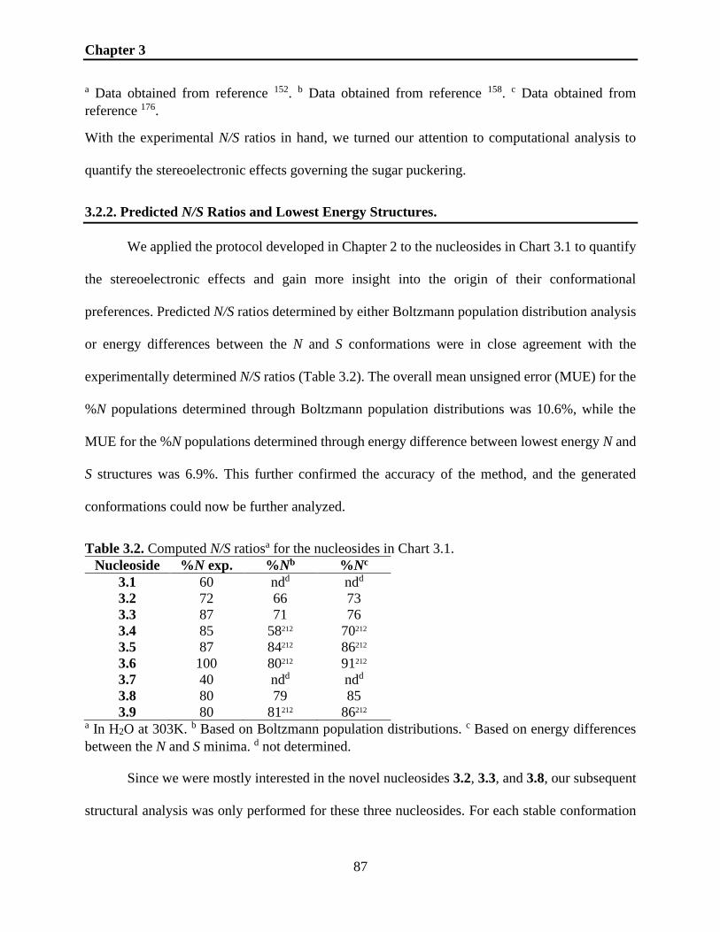
Chapter 3
87
a Data obtained from reference 152. b Data obtained from reference 158. c Data obtained from
reference 176.
With the experimental N/S ratios in hand, we turned our attention to computational analysis to
quantify the stereoelectronic effects governing the sugar puckering.
3.2.2. Predicted N/S Ratios and Lowest Energy Structures.
We applied the protocol developed in Chapter 2 to the nucleosides in Chart 3.1 to quantify
the stereoelectronic effects and gain more insight into the origin of their conformational
preferences. Predicted N/S ratios determined by either Boltzmann population distribution analysis
or energy differences between the N and S conformations were in close agreement with the
experimentally determined N/S ratios (Table 3.2). The overall mean unsigned error (MUE) for the
%N populations determined through Boltzmann population distributions was 10.6%, while the
MUE for the %N populations determined through energy difference between lowest energy N and
S structures was 6.9%. This further confirmed the accuracy of the method, and the generated
conformations could now be further analyzed.
Table 3.2. Computed N/S ratiosa for the nucleosides in Chart 3.1.
Nucleoside %N exp. %Nb %Nc
3.1 60 ndd ndd
3.2 72 66 73
3.3 87 71 76
3.4 85 58212 70212
3.5 87 84212 86212
3.6 100 80212 91212
3.7 40 ndd ndd
3.8 80 79 85
3.9 80 81212 86212 a In H2O at 303K. b Based on Boltzmann population distributions. c Based on energy differences
between the N and S minima. d not determined.
Since we were mostly interested in the novel nucleosides 3.2, 3.3, and 3.8, our subsequent
structural analysis was only performed for these three nucleosides. For each stable conformation

Chapter 3
88
(i.e. lowest energy conformations in the N and S conformations – Figure 3.2), we determined the
pseudorotational phase angle P and the puckering amplitude Φmax (the maximum degree of pucker)
(Table 3.3).
Figure 3.2. Computed lowest energy structures for A. N conformations: left – 3.2; center – 3.3;
right – 3.8 and B. S conformations: left – 3.2; center – 3.3; right – 3.8.
These parameters would be helpful in comparing the computed structures to X-ray crystallography
data. Once these parameters were collected, we proceeded to analyze the hyperconjugation and
anomeric effects that contribute to sugar puckering.

Chapter 3
89
Table 3.3. Puckering parameters obtained for the lowest energy conformations in Figure 3.2.
Nucleoside Conformation P (°) Φmax (°)
3.2 N 60.54 29.98
S 168.48 41.52
3.3 N 55.63 36.09
S 158.60 28.16
3.8 N 47.24 22.06
S 146.11 17.03
3.2.3. Quantifying Stereoelectronic Effects.
Anomeric and hyperconjugation effects through the means of NBO analysis were evaluated
as described in Chapter 2. The anomeric effect nO4′→σ*C4′OMe/F (Figure 3.3A) favors the N
conformation except for 3.8; the strength of the anomeric effect followed the order 3.3 (P = 55.6°)
> 3.2 (P = 60.5°) > 3.8 (P = 47.2°) (values for the anomeric and hyperconjugation effects in
kcal/mol given in Appendix B). Several factors seem to influence the strength of the anomeric
effect: (a) the puckering amplitude of the sugar ring, with a weaker effect observed for lower
amplitudes for both N and S conformations, (b) the hyperconjugation-accepting ability of the 4′-
substituent, and (c) the P angle, with deviations from ideal envelope conformations associated with
weaker anomeric effects.

Chapter 3
90
Figure 3.3. Stereoelectronic effects in 3.8: (A) depiction of the nO4′ → σ*C4′OMe anomeric effect,
(B) depiction of the σC3′C4′→ σ*C2′H hyperconjugation effect, (C) depiction of the σC3′H3′→σ*C4′OMe
hyperconjugation effect.
In the case of 3.8, a plausible explanation for the S conformation exhibiting a slightly larger
anomeric effect is that the N conformation (P = 47.2°, φmax = 22.1°) deviates from an ideal envelope
conformation (P = 54°, φmax = 25−45°). This leads to a poor overlap between the lone pair on the
anomeric oxygen and σ*C4′OMe due to orbital misalignment. However, 3.8 was shown to be
predominantly in the N conformation, and as such, another electronic effect apart from the
anomeric effect should be the driving force behind the observed conformation. Indeed, the data in
Appendix B suggest that the σC3′H3′ →σ*C4′OMe hyperconjugation effect (Figure 3.3C) is the most

Chapter 3
91
pronounced computed electronic effect (with an energy difference of ∼1.9 kcal/mol in favor of the
N conformation), similar in strength to that of 3.2 (∼2.0 kcal/mol) and 3.3 (∼3.1 kcal/mol).
Interestingly, this effect is exhibited in conjunction with a σC3′C4′ → σ*C2′H hyperconjugation effect
(Figure 3.3B) (∼0.8 kcal/mol in favor of the S conformer) that is significantly lower than that
observed for 3.3 (∼3.5 kcal/mol) and 3.2 (∼2.2 kcal/mol), most likely afforded by the orientation
of the fluorine in the arabino configuration. As such, the loss of an important hyperconjugation
effect favoring the S pucker (σC3′C4′ → σ*C2′H), coupled with a strong hyperconjugation effect
favoring the N pucker (σC3′H3′ →σ*C4′OMe), contributes to the observed N conformation of 3.8.
3.2.4. Comparing Computed and Crystal Structures.
The structures of 3.2 and 3.3, first described in this study, were unambiguously confirmed
by X-ray crystallography. Additionally, we obtained the crystal structures of previously reported
3.5 and 3.6.212 These were compared to their predicted conformations by computational analysis,
and the superposition of these are shown in Figure 3.4. 3.3 was crystallized in its most stable
conformation (P1 = 22.4°, Φ1, max= 34.1°, P2 = 21.2°, Φ2, max= 33.8°). In the case of 3.5 (4′-exo), two
slightly different conformations appeared in the asymmetric unit crystal (P1 = 62.3°, Φ1, max = 36.6°,
and P2 = 60.5°, Φ2, max = 37.1°). However, the orientations of the base and the 3′- and 5′-hydroxyls
differ from the computational data. In contrast, 3.2 and 3.6 were crystallized in the S conformation
(P = 163.2°, Φmax = 39.5°) and the E conformation (P = 74.7°, Φmax = 35.4° 28), respectively. It is
important to note that the conformations in which these nucleosides were crystallized do not
necessarily represent the conformations in solution. As discussed in Chapter 2, crystal packing and
intermolecular hydrogen bonding interactions between molecules in different unit cells likely
affect the conformation of the nucleoside in the crystal.213 However, although the positions of
hydrogen-bond accepting/donating substituents on the ring differs between solution and crystals

Chapter 3
92
due to intermolecular hydrogen bonding with solvent/other molecules in the crystal unit, the core
5-membered ring has the same puckering.
Figure 3.4. Superposition between the predicted conformation (green) and the crystal structure
(pink): (A) 3.2, (B) 3.3 (left) unit 1 and (right) unit 2, (C) 3.5 (left) unit 1and (right) unit 2, (D)
3.6.

Chapter 3
93
Overall, the computed structures are in excellent agreement with the crystal structures. One
of the key features to account for when comparing the structures is the heavy atom RMSD.
Importantly, the heavy atom RMSD for all four nucleosides is < 0.8Å (Table 3.5). Moreover, as
can be seen in Figure 3.4, the sugar pucker in all four cases is nearly identical between the
computed and the crystal structures. The major differences that arise between the structures are the
orientations of the substituents, which can be explained through the intermolecular hydrogen
bonding interactions existent in different crystal cells, which affect the orientation of the
substituents containing hydrogen bond acceptors and donors. Nonetheless, in this section we have
shown that the protocol described in Chapter 2 provides invaluable insight into hyperconjugation
effects affecting sugar puckering and highly robust structures that excellently resemble crystal
structures for non-natural nucleosides.
Table 3.4. Heavy atom RMSD between the computed and crystal structures described in Figure
3.4.
Nucleoside Unit Cell Heavy Atom RMSD (Å)
3.2 1 0.47
2 -
3.3 1 0.82
2 0.82
3.5 1 0.51
2 0.59
3.6 1 0.59
2 -

Chapter 3
94
3.3. Atypical Fluorine-Hydrogen Bonds and Their Effects on Nucleoside Conformations.
One of the most important substituents used in controlling ring conformations is fluorine.
Due to its electronegativity, fluorine is an excellent hyperconjugation acceptor (Figure 3.5) and
can thus be used to modulate ring conformations.214,215 Interestingly, fluorine can not only be used
as a hyperconjugation acceptor to modulate conformations, but also as a hydrogen-bond acceptor.
It has been debated for decades whether organic fluorine-hydrogen bonds exist, especially due to
the fact that fluorine rarely accepts hydrogen bonds.216 Moreover, different definitions of what
constitutes a hydrogen bond contribute to this debate – these definitions range from a pure
electrostatic nature of hydrogen bonds, to a combination of electrostatics and polarization effects
as well as a significant covalent bond character.217-219 Irrespective of these definitions, fluorine-
hydrogen bonds can help modulate sugar conformations and thus represent an interesting
component to designing new nucleoside-based drugs.
Figure 3.5. Top. Hyperconjugation in fluorinated pyranose rings. Bottom. Hyperconjugation in
fluorinated furanose rings. The hyperconjugation acceptor (σCF*) is depicted in blue while the
hyperconjugation donor (nO) is depicted in red.
Due to the increasing usage of fluorine in medicinal chemistry applications, several key
pieces of evidence have been found in favour of the existence of fluorine-hydrogen bonds in small
molecules and nucleic acid-based systems.220-222 These recent developments have led IUPAC to

Chapter 3
95
establish guidelines for defining fluorine-hydrogen bonds (Figure 3.6), although different
variations of these parameters have been proposed.223
Figure 3.6. IUPAC guidelines for what constitutes a fluorine-hydrogen bond.
Experimentally, fluorine-hydrogen bonds in nucleosides can be observed by NMR through
scalar JHF coupling.220 This however requires the synthesis of a nucleoside of interest. A cheaper,
more attractive alternative is the computational modeling of nucleosides in which fluorine-
hydrogen bonds are possible. As such, we posited that the protocol developed in Chapter 2 would
be suitable for analyzing nucleosidic fluorine-hydrogen bonds in solution.
3.3.1. Nucleosides That Can Potentially Exhibit Fluorine-Hydrogen Bonds.
It is currently understood that C-F∙∙∙H hydrogen bonds are present in oligonucleotides and
can offer additional stability to the overall structure.183 For example, the hybridization of 2′-F-
ANA oligonucleotides with complementary RNA strands results in the formation of close C-F∙∙∙H
contacts.224 Evidence for these bonds arises from C-F∙∙∙H contacts observed through nuclear
Overhauser effect (NOE) experiments, conformational analysis, and theoretical calculations of
binding free energies.225 On the other hand, 2′-F-araA (Chart 3.2, 3.10) is also hypothesized to
have a C2′-F∙∙∙H8-C interaction based on 1H-NMR and deuterium exchange studies.224 Several
nucleosides,226,227 and more recently, 6′-F-tricyclo-thymidine (6′F-tcT),228 have been proposed to
engage in a similar interaction (Chart 3.2, 3.15). Methods for detecting these interactions in non-
nucleic acid based systems are well developed.220 However, it is less well understood why these

Chapter 3
96
weak intramolecular interactions form and how they influence nucleoside and nucleic acid
structure and stability.
Chart 3.2. Fluorinated nucleosides in which fluorine-hydrogen are hypothesized to occur. The
fluorine and hydrogen atoms between which a hydrogen bond is possible are highlighted in red.
Herein, we examine nucleosides 3.10-3.14 via NMR, X-ray crystallography, and computational
studies. Understanding whether C-F∙∙∙H hydrogen bonds play a role in the conformation and
stability adopted by these systems is important and could lead to the design of new modified
nucleosides that incorporate these interactions.
3.3.2. Analysis of Nucleosides 3.10-3.13.
In D2O, 2′-F-arabinonucleosides (3.10-3.13) exhibit similar sugar conformations, with a
N/S pucker ratio of approximately 2:3 in all cases (Table 3.5). Moreover, since these nucleosides
are in a N/S equilibrium, they pass from one conformation to another through the E conformation
(Figure 2.2). Experimentally, the E conformation is most clearly established through H1′-H4′ NOE

Chapter 3
97
contacts and can cause reduced 3JH1′-H2′.155 Evidence for the existence of the E conformation shows
that; for example, 3.12 exhibits stronger H1′-H4′NOE contacts than 3.13, and thus exhibits a
stronger preference for the E conformation.155 The calculations of these contacts, along with 1H-
19F two-dimensional heteronuclear NOE (HOESY) NMR experiments, show that for nucleosides
3.10-3.13 the distance between the fluorine and hydrogen depicted in red in Chart 3.2 varies
between 2.4 – 2.7Å (Table 3.5, Figure 3.7 – computed lowest energy structures and predicted
distances for nucleosides 3.10 and 3.12).
Table 3.5. Experimental and predicted N/S ratios along with experimental and predicted distances
between the fluorine and hydrogen atoms.
Nucleoside Exp. N/S Pred. N/Sa HOESY Distance
(Å)
Predicted Distance
(Å)
3.10 41/59 47/53 2.5 2.7
3.11 41/59 48/52 2.4 2.7
3.12 38/62 45/55 2.7 2.9
3.13 40/60 60/40212 2.7 2.7
3.14 70/30 60/40 2.3 2.3 a based on Boltzmann population distributions.
Figure 3.7. Lowest energy conformations for 3.10 and 3.12. C-F∙∙∙H-C distance shown with
dashed line. θ is the value of the F∙∙∙H-C angle.
As can be seen in Table 3.5, the N/S ratios are in very close agreement between
experimental and predicted values. Moreover, the predicted distances between the fluorine and
hydrogen atoms are within 0.1-0.3Å of the experimentally determined ones. To probe whether
these distances were short enough to enable fluorine-hydrogen bonds for compounds 3.10-3.13,

Chapter 3
98
we examined the splitting of 13C signals of the purine/pyrimidine bases by fluorine (Figure 3.8).
The purine C8/C4 and the pyrimidine C6/C2 carbons are four bonds away from the 2′-F. If the
interactions were purely long-range in nature, similar 4J2’F-C coupling values would be expected.
However, in 3.10, only the C8 shows significant splitting (4 Hz) from 19F (Appendix B). All other
13C signals showed a splitting of 0.5 Hz or less. The same was true for 3.11. For 3.12 and 3.13, we
compared the C2 and C6 signals; splitting of only the latter was observed.
Figure 3.8. Interactions between fluorine and C8/C6 in purine bases, and between fluorine and
C6/C2 in pyrimidine bases.
In addition to the 13C NMR splitting, we explored the signals of H8 and H6 using 1H NMR.
For nucleosides 3.10-3.13, a small splitting of 1.5 and 2.5 Hz was observed, which may suggest
hydrogen bond-mediated coupling with fluorine as previously proposed for nucleosides, duplexes,
and quadruplexes.229,230 To verify whether the protocol we established in Chapter 2 was capable
of identifying these potential hydrogen bonds in compounds 3.10-3.13, we employed our NBO
analysis protocol on the lowest energy structures obtained following our umbrella sampling
simulations. The F∙∙∙H-C angles for the four compounds were 86°, 54°, 75° and 76° respectively,

Chapter 3
99
which fall outside the typical range of 110-180° necessary for fluorine-hydrogen bonding to occur
(Figure 3.6). However, due to the nature of hydrogen bonding, we posited that electrostatic
interactions might still be possible due to the short distance between the fluorine and hydrogen
atoms. Our NBO analysis however revealed no attractive interaction between the two atoms.
3.3.3. Analysis of Nucleoside 3.14.
Next, we turned our attention to nucleoside 3.14. This nucleoside is analogous to the
previously reported branched nucleoside 3.16 (Figure 3.9),231 which was predicted by DFT
calculations and MD simulations to engage in a weak intramolecular C(sp3)-H∙∙∙F bond between
the hydrogen atom of the 4′-C-CH2 group and F2′.231 Given their similarity and the greater
electronegativity of O vs N, 3.14 was expected to exhibit the same interaction.
Figure 3.9. Analogue of 3.14 that is hypothesized to show a C(sp3)-H∙∙∙F bond.
After synthesizing 3.14, we managed to obtain its crystal structure. This compound
crystallized in its most stable N conformation (P=49.5º). The puckering angle was in very close
agreement with the one obtained for the lowest energy predicted structure of 3.14 (P=52.1º).
Overlay of the two structures revealed a heavy-atom RMSD of 0.78Å (Figure 3.10), while an
analysis of the predicted N/S ratios shows very close agreement to experimentally obtained ones
(Table 3.5).

Chapter 3
100
Figure 3.10. Left: Superposition of crystal structure of 3.14 (green) and predicted structure (pink).
Right: 2D representation of the N conformation for 3.14. Predicted distance (green) between 2′F-
H6′ is 2.3Å, while the C6H6′-2′F angle (purple) is 125.4°.
Importantly, several conclusions can be drawn after analyzing the experimental and
predicted data. First, the predicted lowest energy structure is in excellent agreement with the crystal
structure of 3.14, which gives us confidence that the orientation of the substituents is correct in the
predicted structure. Second, the parameters established in Figure 3.6 are fulfilled when considering
the predicted structure, which shows a H6′-2′F distance of 2.3Å, and a C6H6′-2′F angle of 125.4°.
Combined, these conclusions allow us to posit that a C6H6′∙∙∙2′F interaction is indeed possible. To
verify this, we plotted the electron density and molecular orbitals for the N conformer (Figure
3.11).

Chapter 3
101
Figure 3.11. Top: 2′F-H6′ electron density overlap observed in the N conformation of 3.14.
Bottom: Attractive orbital overlap between 2′F-H6′ in the N conformation.
As can be seen in Figure 3.11, it is clearly visible that an attractive interaction between 2′F
and H6′ exists. As such we proceeded to quantify this interaction through NBO analysis, which
yielded a strength of 0.74 kcal/mol for the C6H6′∙∙∙2′F hydrogen bond. Given the relatively weak
interaction quantified by NBO, we were interested in determining the nature of this bond. To
achieve this, we employed quantum theory of atoms in molecules (QTAIM) analysis. Briefly,
QTAIM explores the idea that chemical bonds can be expressed in terms of the topology of the

Chapter 3
102
molecular electronic density. More specifically, the space occupied by a molecule is divided into
“basins” (or atoms), which are connected through interatomic surfaces (IAS). If these basins
interact through an attractive force, a bond critical point (BCP) in the electron density can be found
and the two basins are said to be connected through a bond path (BP).232 Moreover, at the BCP,
the gradient of the electron density is 0. Importantly, QTAIM can be applied to any system in
which both covalent and non-covalent interactions occur. In 1995, Popelier established that the
existence of IAS, BCP, and BP between a hydrogen-bond donor and acceptor were sufficient to
assert the existence of a hydrogen bond.233 We analyzed the N conformation of 3.14 and we
identified a BCP, BP, and IAS (Figure 3.12), confirming that between C6H6′∙∙∙2′F there was indeed
a hydrogen bond that was most likely electrostatic in nature.234
Figure 3.12. QTAIM BCP (yellow balls) and BP (dashed lines) showing the attractive interactions
between atoms.
To verify whether the predicted C6H6′∙∙∙2′F hydrogen bond could be distinguished
experimentally, we subjected nucleoside 3.14 to [19F-1H] heteronuclear multiple bond correlation
(HMBC) NMR experiments. These experiments showed that the JH6′ -F coupling was in the range
of 1Hz, and that it primarily occurred through-bond rather than through dipole-dipole interactions.

Chapter 3
103
3.4. Conclusions.
In the first part of this chapter we focused on three novel nucleosides containing electron-
withdrawing substituents in key positions on the sugar ring: 2′,4′-diOMe-rU, 2′-OMe,4′-F-rU, and
2′-F,4′-OMe-araU. Conformational analyses of these nucleosides and comparison to other
previously reported 2′,4′-disubstituted nucleoside analogues make it possible to evaluate the effect
of fluorine and methoxy substitution on the sugar pucker, as assessed by NMR, X-ray diffraction,
and computational methods. We found that in all cases the electronegative substituents promote
the N conformation of the sugar puckers. Moreover, we were able to quantify the anomeric and
hyperconjugation effects that arise from the excellent orbital overlaps afforded by the N
conformation when using good hyperconjugation acceptors (-F, -OMe) at key positions (2’ and 4’)
on the sugar ring.
In the second part of this chapter we directly probed the existence of fluorine-hydrogen
bonds in nucleosides using NMR experiments and computational modeling studies in a series of
C2′-fluorinated nucleosides. Specifically, QM/MM analysis and [19F-1H]-HMBC NMR
experiments provided important support for a C-H∙∙∙F hydrogen bond in a 2′-F,4′-C-α-
alkylribonucleoside analogue. This interaction was also supported by QTAIM and NBO analyses
which suggested that a C-H···F interaction (0.74 kcal/mol) indeed exists. In contrast, while
conformational analysis and NMR experiments of 2′-deoxy-2′-fluoroarabinonucleosides indicated
a close proximity between the 2′-F and the nucleobase’s H6/8 protons, molecular simulations did
not provide evidence for a C-H∙∙∙F hydrogen bond.
3.5. Methods.
MD simulations were performed according to the protocol described in Chapter 2. Relevant
angle values and bond distances were calculated in Avogadro v1.2.0. 235 as well as the plotting of

Chapter 3
104
molecular orbitals. Visual QTAIM analysis was performed in Avogadro using wavefunction files
obtained with Gaussian16236 at the M06L/def2-TZVP level of theory. Quantitative QTAIM
analysis was performed using the AIMALL237 program on the same wavefunction files used for
visual QTAIM analysis. NBO analysis was performed using the NBO6200 program. Electron
densities were plotted using Molekel,201 while the lowest energy conformation figures were
rendered with Discovery Studio 4.5.238
Chapter 4
105
Chapter 4 – Predicting Cytochrome P450 Inhibition and
Metabolism at the Drug Development Stage
Preface.
Drug design and discovery is a tedious and costly process. In some cases, after a drug has
reached the market, it shows signs of idiosyncratic toxicity, which culminates with drug
withdrawal from the market. This type of toxicity, along with adverse drug reactions, is a major
hurdle in drug discovery and contributes significantly to the costs associated with bringing a drug
to the market. These adverse drug reactions and toxicity primarily arise from phase 1 metabolism,
where metabolic enzymes – Cytochrome P450 enzymes (CYPs) – are responsible for the
metabolism of 75-90% of xenobiotics. Adverse drug reactions enabled by CYPs can result from
two major routes: CYP inhibition and reactive metabolite formation after CYP oxidation.
Currently, expensive laboratory experiments are necessary to determine these types of
toxicity. Importantly, these experiments can be undertaken only after a compound has been
synthesized or purchased. To reduce the number of drugs that are withdrawn from the market and
to allow the synthesis of drug-like molecules that lack CYP toxicity, we set out to use QM
calculations, docking and ML models to build a tool capable of distinguishing between potential
inhibitors and non-inhibitory molecules before synthesis is even attempted. Moreover, we aimed
to improve our SoM prediction tool IMPACTS to better describe the oxidation products obtained
following a drug’s metabolism by CYPs.

Chapter 4
106
This chapter is partially based on the work presented in the following papers/manuscripts:
Burai Patrascu, M.;‡ Plescia, J.; Kalgutkar, A.; Mascitti, V.; and Moitessier, N. Arkivoc, 2019,
part IV, 280-298.
All authors contributed to writing the manuscript (invited review).
Burai Patrascu, M.;‡ and Moitessier, N. 2020. Improvement of the IMPACTS Drug Metabolism
Tool. – Manuscript in Preparation.
MBP and NM designed the computational experiments. MBP developed the SASA
correction and implemented it in FORECASTER. MBP performed all calculations and analyzed all
the data. MBP and NM contributed to writing the manuscript.
‡ first author
Abstract.
Adverse drug reactions (ADRs) and toxicity are major causes of the high attrition rates
observed in drug discovery and development programs. These adverse reactions generally occur
after phase I metabolism, where cytochrome P450 enzymes (CYPs) metabolize approximately
90% of xenobiotics. Often, these xenobiotics can either inhibit CYPs, or be metabolized into
reactive metabolites that can further interact with DNA and proteins. Experimentally determining
whether a xenobiotic metabolized by CYP enzymes can be toxic/an inhibitor is expensive and
time-consuming. Most importantly, it requires that the xenobiotic be already synthesized.
Computational prediction of CYP toxicity constitutes a viable and more time-efficient alternative.
We have developed a computational tool that relies on QM calculations, docking and ML models
to predict CYP inhibition at the drug development stage. Moreover, to better describe the binding
of drugs to CYPs and identify whether a xenobiotic can be metabolized into a reactive metabolite,
we made significant improvements to our SoM prediction tool IMPACTS.

Chapter 4
107
4.1. Introduction.
Adverse drug reactions (ADRs) and toxicity are major causes of the high attrition rates
observed in drug discovery and development programs. Severe and even fatal toxic effects have
resulted in drug withdrawals, resulting in an enormous financial burden despite huge investments
in toxicology and clinical trials. Although the primary causes of toxicity could be very different,
the first pass bioactivation by metabolic enzymes such as CYPs is often the initiating step. The
produced reactive metabolite further reacts with biomolecules such as proteins, DNA, or
glutathione, leading to hepatotoxicity or DNA mutations causing cancer. Similarly, the co-
administration of drugs with one inhibiting the CYP(s) involved in the metabolism of the other(s)
may lead to the accumulation of the unmetabolised drug(s) resulting in severe toxicity. This
process is known as drug-drug interactions (DDI). Medicinal chemists have relied on “structural
alerts”: functional groups known to possess high toxicity potentials, to flag potentially toxic drug
candidates. Computational prediction of reactive metabolites and DDIs constitutes a viable and
more time-efficient alternative.
4.2. Drug Metabolism, Bioactivation and Toxicity.
Most of the administered drugs are metabolised in the liver to be more efficiently excreted
from the organism. In phase 1 metabolism, the molecules are modified by a set of enzymes,
primarily oxidases and hydrolases. Numerous drugs currently on the market are metabolized by
one of the 57 human CYPs. Out of this set of oxidases, six (CYP1A2, 2C9, 2C19, 2D6, 1E2, and
3A4), expressed mainly in the liver and in the gut, are responsible for more than 90% of this
oxidative metabolism and represent the main focus of medicinal chemists and
pharmacologists.67,239,240 The oxidative metabolism of drugs by CYPs occurs by the means of
heme-mediated oxidation (Chapter 1, Scheme 1.9).

Chapter 4
108
In phase 2 metabolism, the drug (or the metabolite from phase 1) is conjugated to water soluble
moieties (e.g., glucuronic acid), which facilitates its detoxification from the body. The metabolites
produced in this process have their intrinsic pharmacologic effect and toxicity that may differ from
the parent drug. More specifically, they can have longer periods of persistence in the CYP as
inhibitors due to significant intrinsic chemical reactivity, which may result in cell damage. They
can also exhibit high reactivity leading to hepatotoxicity and/or cancer and are referred to as
reactive metabolites. The impact of reactive metabolites and ADR on drug toxicity and drug
withdrawal has been extensively discussed in the literature.241,242 About 75% of the drugs
withdrawn due to ADRs were in fact activated into reactive metabolites.27
While there are several medium throughput techniques available, access to higher
throughput techniques would enable medicinal chemists to make more informed decisions at early
stages of the drug design and development process.243 For instance, predicting the site of
metabolism (SoM), binding mode of small molecules in the CYPs and inhibitory activity of drugs
and their metabolites could be useful to (1) flag potential in vitro hits, (2) help prioritize
experiments, (3) provide key insights enabling the design of compounds with modulated half-life,
(4) predict potentially toxic metabolites, (5) predict potential CYP inhibitors or even (6) predict
the effect of CYP polymorphism (i.e., inter-individual variability).244 A number of computational
approaches have been developed to tackle the challenges associated with drug metabolism and
these include both LBDD and SBDD methods.245-247 Among these approaches is IMPACTS (In-
silico Metabolism Prediction by Activated Cytochromes and Transition States), a fully automated
program developed by the Moitessier group at McGill University, which combines molecular
docking, ligand reactivity estimation, and transition state (TS) structure prediction to predict the
SoMs of drugs metabolized by CYPs. IMPACTS has been shown to accurately predict the SoMs of

Chapter 4
109
over 600 drugs spanning 4 major CYP isoforms.248 Moreover, its implementation in the drug
discovery platform FORECASTER (also developed by the Moitessier group) makes it highly
appealing to medicinal chemists. However, at this current stage, IMPACTS is unable to predict
whether a drug or its metabolites can inhibit CYPs or not.
4.3. CYP Inhibition - Background.
The co-administration of drugs may result in DDIs, due to the ability of a drug to inhibit a
CYP isoform involved in the metabolism of another drug. This leads to the accumulation of the
unmetabolised drug(s) in the human body, causing potentially fatal side effects. CYP inhibition
can either be reversible, quasi-irreversible and irreversible, with the most prevalent form being
reversible inhibition.249 Usually, reversible inhibition occurs when the so-called Type II ligands
(typically molecules containing basic nitrogen atom(s))250 coordinate to the heme iron (Figure 4.1).
An important example of such a ligand is ketoconazole, an antifungal compound that inhibits
CYP3A4 (Figure 4.2). In the case of quasi-irreversible and irreversible inhibition, at least one
catalytic cycle is required for the formation of reactive metabolites that will then interact with the
heme moiety.249
Figure 4.1. a. Reversible CYP inhibition. b. Quasi-irreversible CYP inhibition (MC = metabolic
intermediate complex). c. Irreversible CYP inhibition (RM = reactive metabolite).

Chapter 4
110
Quasi-irreversible CYP inhibition requires the formation of a metabolic intermediate complex
(MC), which can be displaced by in vivo incubation with compounds that have high affinity for
CYP enzymes. Examples of drugs that inhibit CYPs quasi-irreversibly are erythromycin and
lapatinib.251,252 For irreversible inhibition, a reactive metabolite (RM) can either alkylate the heme
(for example by adding to the double bonds – see Figure 4.1c) or interact with key residues in the
CYP active site i.e. acylation of a critical lysine residue by chloramphenicol is well documented.253
Both these mechanisms inactivate the protein, which is then incapable of performing its biological
function. To restore enzyme function, biosynthesis of new enzymes is required.
Figure 4.2. Reversible CYP inhibition of CYP3A4 by ketoconazole. Protein Data Bank (PDB)
code: 2V0M. Active site snapshot. Ligand carbons are shown in purple; heme iron is shown in
orange.

Chapter 4
111
CYP inhibition is a major topic in drug discovery and has been the focus of several
inhibition prediction studies. While quasi-irreversible and irreversible inhibition can be predicted
through SoM methods (by identifying the formation of potential RMs), reversible CYP inhibition
must be treated separately. To understand the importance of reversible CYP inhibition, one can
refer to the study by Vitaku et al.254 that showed that 84% of FDA approved drugs contain at least
one nitrogen atom, with 59% containing at least one nitrogen-containing heterocycle. Thus, there
is a possibility that some of these drugs are Type II ligands that can inhibit CYPs.
Although there are several approaches reported in the literature for predicting reversible
CYP inhibition, particularly based on ML algorithms,255,256 these do not offer insight on the heme-
ligand binding profiles and are not generally transferable (i.e. their quality depends on the chemical
space explored for the training set). In addition to ML methods, docking has also been used to
investigate reversible CYP inhibition. The main advantage of docking methods over ML methods
in this particular case is the ability to visualize the interactions between the ligand and the heme,
which would allow medicinal chemists to undertake any changes necessary to a potential drug to
modulate its binding to CYPs. Moreover, docking allows an isoform-specific description and
visualization of CYP inhibition. For example, it is known that CYP1A2, which accounts for
approximately 15% of the total CYPs, preferentially oxidizes aromatic hydrocarbons and
heterocyclic and aromatic amines due to its narrow active site.243 Such information is highly useful
when developing an inhibition model, since it captures essential enzymatic properties.
The key to determine heme-drug binding energy in docking is to appropriately evaluate the
iron-ligand binding process (coordination). Most commonly used docking programs do not model
the heme-nitrogen coordination explicitly and are thus unsuitable for predicting CYP inhibition
for Type II ligands. To the best of our knowledge, EADock is the only program which has been

Chapter 4
112
trained to predict heme coordination, although the accuracy of 62% (31/50 heme structures that
exhibited iron-nitrogen coordination) remains low.257 Therefore, a framework to predict iron
coordination and displacement of water when localized within a heme is required (in the CYP
resting state there is a water molecule that acts as a distal heme ligand). Herein we set out to
develop a novel predictor of reversible CYP inhibition and implement it in the drug discovery
platform FORECASTER. This tool combines accurate high-level QM calculations on model systems
with the predictive power of the docking program FITTED. Moreover, to complement these tools,
we sought to build an artificial neural network (ANN) capable of analyzing thousands of data
points and to provide accurate predictions on whether a drug or its metabolites can be a reversible
CYP inhibitor. To understand the power of this approach, a drug design and design project such
as the one presented in Figure 4.3 can be undertaken completely within FORECASTER, without the
need for costly HTS.
Figure 4.3. A typical drug design and development project that can be undertaken in FORECASTER.

Chapter 4
113
It is important to note that the time-consuming QM calculations need only be performed once for
the development of the model, which will be described in detail below. The entire in silico part of
the workflow presented in Figure 4.3 can be resolved in a matter of weeks starting from a library
of > 500,000 molecules, which could tremendously speed up the development process of a novel
drug.
4.4. CYP Inhibition – Model Development – Preview.
Since the model we proposed has three distinct phases – QM calculations, docking and
ANN development – we outlined the protocol required for each phase (Figure 4.4).
Figure 4.4. Protocol for developing a reversible CYP inhibition model to be implemented in
FORECASTER.
As can be seen in Figure 4.4., each of these phases is comprised of multiple steps which must be
tackled sequentially to ensure a robust model is built.

Chapter 4
114
4.4.1. CYP Inhibition – Model Development – QM – Step 1.
A significant percentage of FDA approved drugs contain nitrogen heterocycles which
could be capable of coordinating to the iron atom of the heme moiety. We proposed to compile a
list of nitrogen heterocycles bearing various substituents and nitrogen hybridizations that cover as
much of the chemical space as possible (Chart 4.1). This chart was also built based on the data we
acquired from the PDB (Table 4.1) for CYP isoforms with resolution better than 2.5Å. These
heterocycles represent our model systems for Type II ligands.
Chart 4.1. Set of nitrogen-containing heterocycles used as model systems for Type II ligands. The
binding nitrogen atom is depicted in red.

Chapter 4
115
Table 4.1. Data acquired from the PDB for CYP isoforms with resolution better than 2.5Å that
contain iron-coordinating nitrogen ligands.
Entry PDB Code Resolution Isoform Fe-Coordination Nitrogen Hybridization
1 1e9x 2.10 CYP51 yes sp2
2 1ea1 2.21 CYP51 yes sp2
3 1pha 1.63 CAM yes sp2
4 2fdw 2.05 2A6 yes sp3
5 3e6i 2.20 2E1 yes sp2
6 3ibd 2.00 2B6 yes sp2
7 3mdr 2.00 46A1 yes sp3
8 3mdt 2.30 46A1 yes sp2
9 3mdv 2.40 46A1 yes sp2
10 3nxu 2.00 3A4 yes sp2
11 3qoa 2.10 2B6 yes sp2
12 3r9c 2.14 164A2 yes sp2
13 3swz 2.40 17A1 yes sp2
14 3t3q 2.10 2A6 yes sp2
15 3t3r 2.40 2A6 yes sp2
16 3t3z 2.35 20 yes sp2
17 3tbg 2.10 2D6 yes sp2
18 3tjs 2.25 3A4 yes sp3
19 4d75 2.25 3A4 yes sp2
20 4eji 2.10 2A13 yes sp2
21 4fia 2.10 46A1 yes sp
22 4k9w 2.40 3A4 yes sp2
23 4uhi 2.05 CYP51 yes sp2
24 4xrz 2.40 2D6 yes sp2
25 5ese 2.20 CYP51 yes sp2
26 5esf 2.25 CYP51 yes sp2
27 5esh 2.15 CYP51 yes sp2
28 5hs1 2.10 CYP51 yes sp2
29 5irq 2.20 17A1 yes sp2
30 5k7k 2.30 2C9 yes sp2
31 5tz1 2.00 CYP51 yes sp2
32 5uys 2.39 17A1 yes sp2
33 5vce 2.20 3A4 yes sp2
34 6bcz 2.23 3A4 yes sp2
35 6bd7 2.42 3A4 yes sp2
36 6bd8 2.38 3A4 yes sp2
37 6bdh 2.25 3A4 yes sp2

Chapter 4
116
As can be seen in Chart 4.1, the set is comprised of a combination of five and six membered
rings, both aromatic and aliphatic. In the case of six membered aromatic rings, we were interested
in studying how different substituents affect the binding nitrogen reactivity, and, as such, we
ensured that these rings contained both EWG and EDG in the ortho, para, and meta positions. In
contrast, in the case of five membered aromatic rings, we wanted to study whether different
heteroatoms in the heterocycle would enhance or decrease nitrogen binding to iron and so we
looked into various combinations of heterocycles containing two, three or four heteroatoms.
4.4.2. CYP Inhibition – Model Development – QM – Step 2.
Because the iron-nitrogen coordination process is highly dynamic and requires
consideration from both steric and electronic effects, we decided to capture the energetics of this
process using QM calculations. Several aspects were considered before the start of the PES
calculations for the ligands in Chart 4.1 and are outlined further. a) Since docking is a static process
and the mobility of the heme moiety cannot be modeled with FITTED, we decided to undertake all
our QM calculations with a pre-optimized truncated heme moiety that would not be further
optimized during the iron-nitrogen coordination process of the ligands in Chart 4.1. The carboxylic
acid, methyl, and terminal ethylene chains were removed to reduce computational cost. This
approach eliminates heme mobility as a variable from developing a new MM potential for the iron-
nitrogen coordination process. b) To obtain an optimized heme structure that was suitable for the
coordination process of all ligands in Chart 4.1, we used the most sterically hindered ligand (4.18,
Chart 4.1) in the optimization process. This ensures that the heme structure used during the iron-
nitrogen coordination process of the ligands in Chart 4.1 sterically allows all ligands to bind. The
optimized heme structure used in all PES calculations is shown in Figure 4.5. c) To determine
what level of theory was suited for the PES calculations, we used compound 4.14 as a benchmark

Chapter 4
117
ligand. For this purpose, we tested several methods (see section 4.6 for full description of
methodology) and we observed that a PBE0(D3BJ)/def2-SVP/ LANLDZ(Fe) level of theory
offered the most accurate and cost-efficient approach.258 d) Once steps a-c) were completed, we
investigated the computational conditions necessary for obtaining relevant PESs for the iron-
nitrogen binding process. Since we were interested in the formation of the iron-nitrogen bond, we
decided to perform unidimensional PES scans where the coordinate used in the scan was the iron-
nitrogen bond distance. The distance was varied from 10Å – where there is no interaction (or very
little) between the ligand and heme – to 1.6Å – where there is a repulsion between the iron and
nitrogen – in increments of 0.2Å, thus obtaining 43 unique structures across the PES. At every
point on the PES, the ligand was optimized while the heme was kept frozen at the pre-optimized
geometry.
Figure 4.5. Left) Optimized heme-4.18 complex. Ligand carbons shown in purple. Right)
Optimized truncated heme moiety used in obtaining the PES scans. Hydrogens omitted for clarity.
Cysteine residue is represented by -S-Me. Iron atom is shown in orange.

Chapter 4
118
For each of the ligands presented in Chart 4.1 the protocol described at point d) was carried
out. As an example, the full PES scan of ligand 4.1 is presented in Figure 4.6 along with snapshots
of the binding process at 10.0 (no interaction), 2.0 (minimum) and 1.6Å (repulsion) (purple dots).
The PES scans of the other ligands in Chart 4.1 are given in Appendix C.
Figure 4.6. PES scan showing the binding process of ligand 4.1 to heme. Snapshots are given at
an iron-nitrogen distance of 10.0, 2.0 and 1.6Å. Ligand carbons are colored in purple. Hydrogens
omitted for clarity.
Importantly, the PES scans revealed that for compounds 4.7, 4.8 and 4.30 the binding process is
unfavorable. In all three cases, the binding process led to highly distorted ligand structures, which

Chapter 4
119
contributed to the instability of the final complex. These compounds were not considered in the
development of the new MM potential.
4.4.3. CYP Inhibition – Model Development – Docking – Step 1.
With the QM data in hand, we thought to develop a new MM potential to be implemented
in FITTED. Since van der Waals (vdW) interactions are described in FITTED using a Lennard-Jones
12-6 (LJ(12-6)) potential (see Equation 1.8), the first step was to obtain the FITTED energy profile
for the same 43 unique structures used in section 4.4.2. An overlay of the energy profiles obtained
with QM and FITTED for compound 4.1 is given in Figure 4.7 (orange curve).
Figure 4.7. Overlay of QM and FITTED energy profiles obtained for compound 4.1.
As can be seen in Figure 4.7, the LJ(12-6) potential is unable to describe the iron-nitrogen
coordination process. As such, the development of a new LJ potential, similar to the one we had
-60
-40
-20
0
20
40
60
80
0 2 4 6 8 10 12Ener
gy (
kcal
/mo
l)
Fe-N Distance (Angstrom)
DFT
LJ(12-6) Potential
LJ(8-4) Potential
LJ(6-3) Potential
LJ(8-4) Potential With Offset

Chapter 4
120
previously developed for zinc coordination, was necessary. In this context we decided to verify
whether two of the most commonly used LJ potentials (8-4 and 6-3, Equations 4.1 and 4.2) could
be able to describe this process better than the LJ(12-6) potential. As can be seen in Figure 4.7, the
LJ(6-3) potential (green curve) describes an energy minimum (~ 37 kcal/mol) that is too low in
energy compared to the QM minimum (~ 28 kcal/mol). Moreover, the iron-nitrogen distance at
which this minimum occurs is offset by 0.4Å when compared to the QM minimum (2.4Å vs 2Å).
EvdW(8−4) = ∑ εij [(Rmin,ij
rij)
8
− (Rmin,ij
rij)
4
]
pairs i,j
Eq. (4.1)
EvdW(6−3) = ∑ εij [(Rmin,ij
rij)
6
− (Rmin,ij
rij)
3
]
pairs i,j
Eq. (4.2)
Equations 4.1-4.2. LJ(8-4) and LJ(6-3) potentials for computing vdW interactions.
In contrast, the energy minimum (~ 31 kcal/mol) described by the LJ(8-4) potential is very
close in energy to the QM one. However, the minimum described by the LJ(8-4) potential was also
offset by 0.2Å when compared to the QM minimum (2.2Å vs 2Å). To verify whether incorporating
the offset in the computation of the LJ(8-4) potential would improve the energy profile described
by FITTED, we plotted the potential containing the offset in Figure 4.7. Interestingly, this led to an
excellent overlap between the QM and FITTED energy profiles, with an overall MAE of 0.63
kcal/mol between the two curves. The necessity of using an offset was not a singular occurrence;
in all cases, we observed that the LJ(8-4) potential required the inclusion of this offset to properly
described the binding process. This led to the implementation of the modified potential shown in
Equation 4.3 into FITTED for describing the iron-nitrogen binding process. Importantly, the overall
Chapter 4
121
MAE across all compounds used in the development of the new potential is 0.66 kcal/mol, which
suggests that FITTED would now be capable to describe the iron-nitrogen binding process with QM
precision at an MM cost.
EvdW(8−4)−FITTED = 4εσ8
(r − 0.2)8−
4εσ4
(r − 0.2)4 Eq. (4.3)
Equation 4.3. Modified LJ(8-4) potential implemented in FITTED. ε – energy minimum obtained
after subtracting the original FITTED profile from the QM profile. σ – distance (in Å) at which there
is repulsion between the iron and nitrogen (in all cases σ = 1.6Å).
4.4.4. CYP Inhibition – Model Development – Docking – Step 2.
In FITTED, users can select two different docking modes depending on the nature of the
protein (normal protein or metalloprotein).259 Depending on the mode of choice, FITTED uses
different conditions for preparing and processing the crystal structures for docking, as well as for
performing docking (different scaling terms for non-covalent interactions, including different LJ
potentials for vdW interactions). Thus, the new LJ(8-4) potential was implemented only in the
metalloprotein mode of FITTED. Afterwards, we assembled a representative set of CYP-ligand
complexes from the PDB in order to perform a self-docking study for both protein and
metalloprotein docking modes. This set is comprised of 85 diverse crystal structures (see Appendix
C for full list), with and without iron-coordinating nitrogen ligands. Briefly, self-docking assesses
the ability of a docking program to dock a ligand extracted from a crystal structure to that same
crystal structure and compare the RMSD between the docked pose and original crystal structure.
Generally, an RMSD less than 2.0Å between the predicted and crystal structure is considered to
be adequate.

Chapter 4
122
The results of the self-docking study in both docking modes are given in Figure 4.8.
Interestingly, when using the 2.0Å threshold for success of self-docking, there is a minimal
difference between the docking modes (63.5 vs. 61.2% accuracy). This seems surprising,
considering that the original LJ (12-6) did not properly describe the iron-nitrogen coordination
process. However, before any conclusions can be made about the difference in accuracy between
the two docking modes, we must take a closer look at the failures and differences in results and
best binding poses between the two.
Figure 4.8. % accuracy of protein vs. metalloprotein mode in the self-docking of heme proteins.
0
10
20
30
40
50
60
70
80
90
100
0 1 2 3 4 5 6
% A
ccu
racy
RMSD (Angstrom)
Protein vs Metalloprotein Docking Mode
Protein Docking Mode
Metalloprotein Docking Mode

Chapter 4
123
One of the most striking differences in results is for the crystal structure with PDB id 3CZH
(CYP2R1 in complex with Vitamin D2, non-iron coordinating ligand). In the case of the protein
mode, the RMSD was 0.54Å, while for the metalloprotein mode it was 9.45Å (Figure 4.9). As can
be seen in Figure 4.9, vitamin D2 is a large ligand that spans a significant portion of CYP2R1’s
active site. However, although large, vitamin D2 is rigid, containing only 5 rotatable bonds. This
in turn should allow docking to perform well, as evident from the protein mode RMSD. One
possible explanation for the inability of the metalloprotein mode to obtain a better RMSD lies in
the stochastic nature of the docking process. FITTED relies on a genetic algorithm where, at the
beginning of the docking process, an initial population of 100 conformations is generated
randomly. If the ligand is large and/or flexible, then the number of initial conformations should be
increased to explore the conformational space thoroughly. If the number of initial conformations
is too small, then it is likely that a suitable conformation is not found. However, in the interest of
speed vs. accuracy, as well as to be consistent with our previous self-docking studies, we decided
to use 100 initial conformations for all the crystal structures assembled for this self-docking study,
irrespective of the ligand size.
Another example in which the protein (RMSD = 6.30Å) and metalloprotein (RMSD =
0.69Å) modes differ significantly is in the case of the crystal structure with the PDB id 4EJI
(CYP2A13 in complex with an iron-coordinating nitrogen ligand – Figure 4.10). While in the
protein mode the best docked pose suggests the nitroso group to be close to the iron, in the
metalloprotein mode the pyridine nitrogen is correctly bound to the iron. Importantly, the N-Fe
bond length in the crystal ligand is 2.05Å, while the bond length in the best docked pose in
metalloprotein mode is 2.07Å, suggesting that the new LJ(8-4) potential can properly describe
iron-nitrogen coordination.

Chapter 4
124
Figure 4.9. Self-docking results for 3CZH – active site snapshot. Green – crystal ligand; Orange
– protein mode; Yellow – metalloprotein mode. Oxygen atom in ligands are colored red.
Figure 4.10. Self-docking results for 4EJI – active site snapshot. Green – crystal ligand; Orange –
protein mode; Yellow – metalloprotein mode. In the ligands, nitrogen atoms are colored in blue,
while oxygen atoms are colored in red.
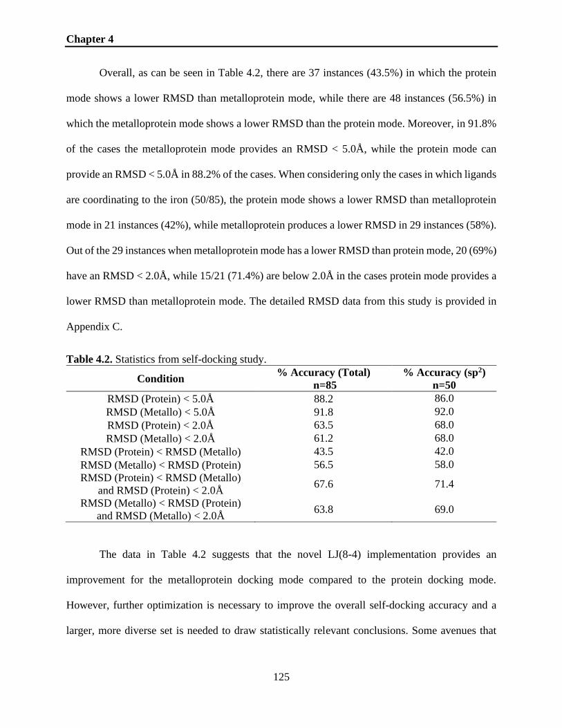
Chapter 4
125
Overall, as can be seen in Table 4.2, there are 37 instances (43.5%) in which the protein
mode shows a lower RMSD than metalloprotein mode, while there are 48 instances (56.5%) in
which the metalloprotein mode shows a lower RMSD than the protein mode. Moreover, in 91.8%
of the cases the metalloprotein mode provides an RMSD < 5.0Å, while the protein mode can
provide an RMSD < 5.0Å in 88.2% of the cases. When considering only the cases in which ligands
are coordinating to the iron (50/85), the protein mode shows a lower RMSD than metalloprotein
mode in 21 instances (42%), while metalloprotein produces a lower RMSD in 29 instances (58%).
Out of the 29 instances when metalloprotein mode has a lower RMSD than protein mode, 20 (69%)
have an RMSD < 2.0Å, while 15/21 (71.4%) are below 2.0Å in the cases protein mode provides a
lower RMSD than metalloprotein mode. The detailed RMSD data from this study is provided in
Appendix C.
Table 4.2. Statistics from self-docking study.
Condition % Accuracy (Total)
n=85
% Accuracy (sp2)
n=50
RMSD (Protein) < 5.0Å 88.2 86.0
RMSD (Metallo) < 5.0Å 91.8 92.0
RMSD (Protein) < 2.0Å 63.5 68.0
RMSD (Metallo) < 2.0Å 61.2 68.0
RMSD (Protein) < RMSD (Metallo) 43.5 42.0
RMSD (Metallo) < RMSD (Protein) 56.5 58.0
RMSD (Protein) < RMSD (Metallo)
and RMSD (Protein) < 2.0Å 67.6 71.4
RMSD (Metallo) < RMSD (Protein)
and RMSD (Metallo) < 2.0Å 63.8 69.0
The data in Table 4.2 suggests that the novel LJ(8-4) implementation provides an
improvement for the metalloprotein docking mode compared to the protein docking mode.
However, further optimization is necessary to improve the overall self-docking accuracy and a
larger, more diverse set is needed to draw statistically relevant conclusions. Some avenues that

Chapter 4
126
could be pursued include the development of optimized heme force field parameters, along with
optimized scaling factors for non-covalent interactions specifically designed for heme proteins.
4.4.5. CYP Inhibition – Model Development – ANN – Steps 1 and 2.
As discussed in Chapter 1 and in one of our recently published reviews,27 an ANN is only
as good as the data used to train it. For CYP inhibition, this is especially true. It is important to
mention that there are several types of assays used to determine CYP inhibition, including
luciferase-based assays260 or LC/MS/MS-based assays261 to determine whether a compound
inhibits a specific CYP. One important characteristic of these assays is that they indiscriminately
detect inhibition, whether it is reversible or irreversible. These assays also measure different
parameters such as AC50 (half maximal activity) or IC50 (half maximal inhibitory concentration)
and have different thresholds for inhibition. Thus, it is paramount to account for different assays
when assembling a training and testing set for determining the accuracy of an ANN. If possible,
the set should contain thousands of data points (both inhibitors and non-inhibitors) and be built
using data obtained with the same type of assay. Ideally, this data should be obtained from one
source, since this would ensure that the data was gathered in the same manner and the systematic
errors would be consistent throughout the assay.
To this end, we built a relevant set of CYP inhibitors that could be used as training and
testing sets for our ANN. Following our literature search, we selected the AID-1851 CYP450 panel
bioassay published on PubChem by the National Center for Advancing Translational Sciences as
the source of our set.262 This is a luciferase-based assay that determines the AC50 of ~17000
compounds in five major CYP isoforms: CYP1A2, 2C9, 2C19, 2D6, and 3A4. Briefly, the assay
measures the dealkylation of various pro-luciferin substrates to luciferin, which is then measured
using luminescence after a luciferase detecting agent has been added. Inhibitors limit the

Chapter 4
127
production of luciferin and decrease the measured luminescence. According to the assay,
compounds with AC50 equal or less than 10 μM are considered active.
As it is the case with most publicly available datasets, we had to curate it to obtain a usable
set of drug-like compounds. Briefly, we initially filtered the 17000 compounds for atoms
commonly found in drugs (C, N, H, O, F, Br, Cl, I, Si, S, P) and then subjected the set to filtering
based on Lipinski’s rule of 5 (molecular weight < 500 Da, hydrogen bond acceptors < 10, hydrogen
bond donors < 5 and a logP < 5). Then, we split the full set into two subsets for each isoform
comprising active and inactive compounds. The final number of compounds per set per isoform is
given in Table 4.3.
Table 4.3. Breakdown of sets per isoform.
Isoform Activity Number of Compounds
Number of compounds containing a
nitrogen atom capable of coordinating
to the heme iron
1A2 active 4453 3330
inactive 6132 2835
2C9 active 2708 1764
inactive 7823 4333
2C19 active 4111 2526
inactive 6580 3535
2D6 active 1905 934
inactive 9953 5862
3A4 active 3118 2182
inactive 6932 3657
For all isoforms, the active and inactive sets were then converted from 2D to 3D using our
program CONVERT and prepared for docking using SMART. SMART is also capable of assigning
atomic and molecular descriptors to compounds, including molecular weight, number of hydrogen
bond donor and acceptors, number of rings and stereocenters, logP (a measure of hydrophobicity),
logS (a measure of solubility in water), topological polar surface area, and number of heteroatoms
(N, O and S). We believed that these descriptors could be as important as the docking data since

Chapter 4
128
they provide essential information about the compounds. As such, after the docking process was
complete, for each active and inactive a detailed breakdown of various energy terms from the best
docking run (vdW, electrostatic, hydrogen bond energy etc.) and a breakdown of descriptors was
output to be further used in the development of the ANN.
4.4.6. CYP Inhibition – Model Development – ANN – Step 3.
There are many flavors of ANNs available in the literature. Amongst these, one of the most
common ones is the supervised ANN using a “back-propagation” algorithm.263 Developed in 1986
by Rumelhart, Hinton, and Williams,264 back-propagation quickly became the algorithm of choice
for ANNs developed in chemistry.
Figure 4.11. A schematic depiction of the back-propagation algorithm. Reproduced from
reference 263.
Briefly, as depicted in Figure 4.11, the input data is delivered through the layers of neurons.
If an ANN has multiple layers, the output data from layer n becomes the input data for layer n+1.
Chapter 4
129
The main goal of such an ANN is for predictive output data to be delivered by the final layer.
However, in the case of back-propagation, this is not the case in the beginning. The final layer will
predict output data, which will then be compared to an expected value, which is known beforehand
(experimental data coming with the dataset). The next step involves computing the error between
the expected and output values by the final layer, which is then used to correct the data from the
final layer using a conjugate gradient method. Subsequently, the weights from the penultimate
layer are corrected with respect to the final layer. This process occurs layer by layer until the input
layer is reached. Thus, the error is propagated backwards from bottom to top and is used to correct
the weights in each layer. The main goal of this algorithm is to minimize the error in the output
layer.
We believed that an ANN using a back-propagation algorithm was robust for our needs,
and thus we implemented it in our drug discovery platform FORECASTER and connected it to our
docking program FITTED. To remove the need for manual intervention in building the training and
testing sets, we decided to automate this aspect as well (although the user can still select the
training:testing set ratio). Afterwards, we opted for a single hidden layer, which would take as
input both the docking and ligand data obtained in section 4.4.6. After building the ANN, we set
out to identify the most appropriate descriptors for evaluating CYP inhibition and we found that
out of 25 distinct descriptors a combination of docking-based energy values (vdW, electrostatic,
hydrogen bond energy, metal coordination, Score and MatchScore) and ligand-based descriptors
(number of rotatable bonds, net charge, number of hydrogen bond donors and acceptors) was
optimal. The Score output by FITTED after docking describes how favorable the electronic
interactions a ligand makes with the amino acids in the active site are, while MatchScore describes

Chapter 4
130
how well a ligand fits inside the active site of an enzyme.265,266 Once these tasks were completed,
we proceeded to assess the accuracy of our ANN in distinguishing inhibitors vs non-inhibitors.
4.4.7. CYP Inhibition – Model Development – ANN – Step 4.
Several aspects must be accounted for when training a ANN. First, the accuracies of both
the training and testing sets must be compared to ensure overfitting did not occur. Second,
important insight into the behaviour of the ANN can be obtained if one computes the specificity
and sensitivity, along with the positive and negative predicted values (PPV and NPV). The
specificity of an ANN in the context of CYP inhibition describes the proportion of molecules
predicted to be inactive among those that are experimentally inactive, while the sensitivity
describes the proportion of molecules predicted to be active among those that are experimentally
active. The PPV describes the probability that a predicted active is experimentally active while the
NPV describes the probability that a predicted inactive is experimentally inactive. In our case, we
computed all these parameters for each specific isoform (Table 4.4).
Table 4.4. ANN results.
CYP Accuracy Sensitivity Specificity PPV NPV
1A2 94.6 91.1 97.2 95.9 93.8
80.6 75.1 84.7 78.2 82.3
2D6 89.3 36.0 99.5 93.7 89.0
85.1 27.4 96.2 57.8 87.4
2C9 93.5 76.9 99.3 97.3 92.6
79.9 49.4 90.5 64.3 83.8
2C19 89.3 79.8 95.2 91.2 88.3
78.3 65.9 86.0 74.8 80.1
3A4 91.6 76.7 97.1 90.8 91.9
80.2 54.4 89.8 66.3 84.2
As can be seen in Table 4.4, the accuracy of the ANN for the training set is excellent.
However, the accuracy of the testing set is lower in all cases, indicating that overtraining has

Chapter 4
131
occurred. Moreover, in the case of CYP 2D6, our ANN performs poorly in terms of sensitivity in
both the training and testing set cases. The same holds true for 2C9 and 3A4 in the case of the
testing sets. It is clear from these results that more work is needed to improve the ANN and to
avoid overfitting. To put the results in Table 4.5 in context, we have assembled data from three
different publications that use the same bioassay to develop machine learning methods that
discriminate between inhibitors and non-inhibitors. These results are given in Table 4.6 and show
that throughout the literature the problem of overfitting seems apparent. Nonetheless, the
foundation of our unique docking-ligand-ML approach to discriminate between inhibitors vs. non-
inhibitors is laid, and further improvements are expected in the future.
Table 4.5. Comparison of our ANN with literature. Accuracies are given for testing and (training)
sets.
Reference 1A2 2C9 2C19 2D6 3A4
Sun et al.267 0.79
(0.93)
0.77
(0.89)
0.86
(0.89)
0.90
(0.85)
0.73
(0.87)
Cheng et al.268 0.73 0.87 0.81 0.88 0.76
Li et al.269 0.97
(0.89)
0.86
(0.86)
0.81
(0.84)
0.89
(0.88)
0.89
(0.85)
Our ANN 0.81
(0.95)
0.80
(0.94)
0.78
(0.89)
0.85
(0.89)
0.80
(0.92)
4.5. SoM Prediction – IMPACTS 2.0 – Background.
For many years, we have been developing accurate software for drug discovery and
development. For instance, in 2012, we developed IMPACTS, a tool outperforming experts in the
prediction of SoM of xenobiotics by CYPs.248 IMPACTS was developed based on the understanding
of the CYP-mediated drug metabolism mechanism. Briefly, IMPACTS, is a hybrid method based on
both ligand docking and ligand activation energies. Prior to docking of a drug-like molecule, the
atoms that could potentially constitute SoMs are assigned pre-computed activation energies,
obtained following the reaction of a set of representative fragments with the active CYP450 species

Chapter 4
132
responsible for oxidation. Then, IMPACTS docks the molecule using routines derived from our in-
house docking program FITTED, creates the likely transition states, and uses the collected
information to decide which SoM will be preferred (Figure 4.13). The original version of IMPACTS
showed an accuracy of 77% across 4 isoforms (CYP1A2, 2C9, 2D6 and 3A4).
With the implementation of our CYP inhibition prediction tool into FORECASTER and
expansion of our drug metabolism-related predictive software, we sought to revisit IMPACTS
through a fresh look at CYP-mediated drug metabolism mechanism in hopes of improving its
accuracy.
Figure 4.12. Automated IMPACTS protocol.
4.5.1. SoM Prediction – Improving IMPACTS – Approach.
As with many enzymatic reactions, the rate of CYP oxidation is driven by 1) stabilization
of the transition state by the enzyme, 2) proper positioning of the reacting partners, 3) substrate
reactivity, and 4) modified kinetics (e.g. first order in enzyme, second order in solution) of the
chemical process. To tackle this problem, the original version of IMPACTS was modeling the
transition state (#1) of the substrate enzyme complex using routines from our docking program

Chapter 4
133
FITTED (#1 and #2) considering the reactivity of each potential reactive SoMs of the substrate from
DFT calculations of fragments (#3) and assuming similar effect of the kinetics on every substrate
(#4). While all these factors were considered, we believed that there was space for improvement.
Over the years, we have found that water molecules and protein flexibility could be critical for
optimal binding mode prediction. We are also aware of the impact of the basis set and functionals
in DFT calculation on the accuracy of the resulting predictions. At this stage, our research focused
on the following factors: 1) an improved docking program (FITTED’s accuracy has improved
throughout the years) including a more accurate consideration of protein flexibility, 2) higher-level
calculations of fragment energy of activation, and 3) additional consideration of steric effects.
The first step of our study consisted in assessing the accuracy of the current version of
IMPACTS on the training set used in 2012. The accuracy values presented throughout this chapter
are average values obtained over five different runs to ensure reproducibility (including standard
deviations). The detailed data obtained from these runs can be accessed in Appendix C. As can be
seen in Figure 4.13, the overall accuracy of IMPACTS has not changed significantly (within 2%
overall). This small variation in accuracy can be attributed to significant changes made to the way
molecules are prepared for docking (correctly treating aromaticity in molecules, proper resonance
structure attribution and improved charging scheme) as well as to the docking process itself
(improved convergence parameters and the nature of the stochastic process of docking). Moreover,
we checked whether reducing the number of available SoM’s prior to docking would improve the
accuracy of IMPACTS. As such, we allowed only the top 5 activation energies to be considered in
the docking process. However, this adjustment did not change the accuracy dramatically (Figure
4.13).

Chapter 4
134
Figure 4.13. Accuracy using the current version of IMPACTS compared to the one determined in
2012.
With these results in hand, we investigated the different aspects presented in our approach to see
whether IMPACTS could be improved.
4.5.2. SoM Prediction – Improving IMPACTS – Ligand Reactivity.
In the past few decades, several developments have been made in the field of chemical
reactivity. Amongst these are chemical reactivity descriptors – computed values that can be used
to determine whether a molecule or an atom in a molecule is reactive.270 Molecular reactivity
descriptors offer information across an entire molecule (i.e. chemical softness, hardness etc.) but
provide no usable information about local sites of reactivity. For example, the HSAB theory
developed by Pearson states that a hard molecule will preferentially react with a hard molecule as
opposed to a soft one.117 In contrast, LARIs have been developed to account for reactivity of
individual atoms. Amongst these are the Fukui coefficients developed in the context of frontier
molecular orbital (FMO) theory. These coefficients offer information about nucleophilic,

Chapter 4
135
electrophilic, and radical attacks and have been discussed in Chapter 1 and thoroughly throughout
the literature. To help with our efforts in the field of drug discovery, we implemented FCs as well
as other LARIs and molecular properties (global hardness, softness, nucleophilicity,
electrophilicity etc.) in the context of both HF and DFT in our QM program QUEMIST (for a
detailed description of the development and implementation of QUEMIST see Chapter 5).
Since the CYP oxidation mechanism proceeds through radical attack on the SoM, we
investigated whether FCs could be used in conjunction with or as a substitution to our activation
energies to provide a more accurate description of the radical attack on potential SoMs.
Preliminary results showed that computationally demanding atom-condensed FCs from Hirshfeld
atomic charges can increase the accuracy of IMPACTS by no more than 2% overall.271 In addition,
a major drawback of this approach is that it requires three separate QM single point energy
calculations for the neutral, anionic, and cationic molecules to obtain the FCs. Moreover, these
coefficients showed a high dependence on the type of atomic charges used (i.e. Mulliken, Hirshfeld
etc.). To offset these drawbacks and to reduce the computational cost associated with computing
FCs, we turned our attention to a method that allows the quantification of atom-condensed FCs
directly from only one QM energy calculation performed on the neutral molecule.272,273 The QM
information (molecular orbitals, orbital energies and overlap matrix) is easily obtained using
QUEMIST. The FC’s are then normalized in the 0-100 range and used automatically within IMPACTS
itself. A comparison between the accuracies obtained in 2012 and 2019 (with and without FCs) is
given in Figure 4.14.

Chapter 4
136
Figure 4.14. Accuracy using the current version of IMPACTS with and without FCs.
As can be seen in Figure 4.14, the usage of FCs (computed at the HF/def2-SVP level of
theory) did not provide the expected accuracy improvement for IMPACTS. A detailed analysis of
the results shows that across all sets the FCs have the highest values on aromatic carbons, which
is consistent with aromatic rings being electron rich. However, this disfavors potential SoMs
represented by sp3 carbons, which generally have a low FC. This fact is particularly evident for
the 2D6 set, which exhibits a high decrease in accuracy due to 72% of SoMs being comprised of
sp3 carbons.
4.5.3. SoM Prediction – Improving IMPACTS – New Activation Energies.
After assessing the usage of FCs in the prediction of SoMs, we posited that the approach
developed in 2012 to assign activation energies could be improved. As such, we embarked on a

Chapter 4
137
journey similar to that expanded in SMARTCyp 3.0274 and decided to improve the assignment of
activation energies through the following protocol:
1. Survey the literature and collect fragments of interest found in drug molecules (i.e.
styrene, thiophene etc.)
2. Design and implement a fragment-matching algorithm that could efficiently
identify fragments of interest in any given drug molecule.
3. For the fragments of interest – obtain TSs at the ωB97X-D3//def2-SVP
(geometrical counterpoise correction - gCP)/def2-SVP (zero-point energy - ZPE) for the reactive
atoms using a methoxy radical model.
4. Assign activation energies during IMPACTS based on the fragment-search protocol.
If the fragment is not found, the activation energy is assigned based on the old protocol. Our
approach led to a set of 156 fragments and over 450 TSs (e.g. o,m,p-substituted aryl fragments
were counted as separate TSs). For the QM calculations, our choice of ωB97X-D3//def2-
SVP(gCP)/def2-SVP(ZPE) level of theory was based on functional quality, speed, and accuracy,275
while the choice of methoxy radical was based on our previous work and that of others.248,276 While
we expected comparable accuracies to the original activation energies, we were surprised to see a
major drop in accuracy (almost 13% overall), especially for 2D6 (Table 4.6). We attributed this to
the relatively small basis set we used to compute the energies, as well as to the fact that due to the
vastness of the chemical space we probably did not cover enough fragments to assign them
properly.

Chapter 4
138
Table 4.6. Accuracy of IMPACTS when using the new activation energies.
Isoform Run 1 Run 2 Run 3 Run 4 Run 5 Overall
Accuracy
Std.
Dev.
1A2 66.4 68.6 69.3 68.6 65.0 67.6 1.6
2C9 70.5 69.0 67.3 67.4 69.8 68.8 1.3
2D6 47.1 48.4 49.7 45.9 51.0 48.4 1.8
3A4 67.2 67.2 65.9 66.9 66.2 66.7 0.5
Moreover, the choice of a methoxy model, while the fastest in terms of speed, precludes the
description of the possible radical spin transfer to the heme iron during the oxidation process.
4.5.4. SoM Prediction – Improving IMPACTS – Steric Effects and Ligand Accessibility.
In our quest to improve the accuracy of IMPACTS we were set on improving the activation
energies obtained in 2012. However, from the investigations described above, the activation
energies were reliable and multiple efforts to further improve them proved to be unfruitful. As
such, we turned our attention to the other aspect of the CYP metabolism, namely sterics. While
the docking routines are considering some of these effects, precluding some unrealistic binding
modes, the intrinsic accessibility of the SoMs was not being addressed. To expand on this, we
decided to “pre-filter” the potential SoMs using a very simple sterics descriptor – solvent
accessible surface area (SASA). We implemented the Shrake-Rupley277 algorithm for computing
SASA in FORECASTER and developed an equation (Eq.4.4) to integrate the sterics descriptor within
the activation energies:
Corrected Eact = Eact − ∆ × SASAatomic Eq. (4.4)
Equation 4.4. Corrected activation energies for IMPACTS. ∆ is a correction factor that has an
optimized default value of 0.1.
This approach would ensure that both intrinsic reactivity and accessibility would be accounted for
at the moment of docking with IMPACTS. The results of this approach are presented in Figure 4.15.

Chapter 4
139
Figure 4.15. Accuracy using the current version of IMPACTS with and without SASA.
Figure 4.15 shows that the accuracy for each isoform increases significantly when adding
the SASA correction. Overall, the accuracy of IMPACTS increases by almost 5% to when compared
to the data in Figure 4.13 (80% overall). The decision to limit the number of SoM’s for docking to
5 proved to be an inspired one in this case, since this condition shows the highest accuracy overall
(Figure 4.15).
4.5.5. SoM Prediction – Improving IMPACTS – IMPACTS 2.0.
To test whether the data in Figure 4.15 was consistent across different sets, as well as across
different isoforms that were not involved in the initial testing procedure, we assembled new sets
for CYP1A2, 2C9, 2C19, 2E1, and 2D6 totaling 1125 drug molecules. The results in Figure 4.16
show that our SASA correction approach improves the accuracy of the overall set by 3%.
Importantly, the use of SASA correction brings all isoforms over 70% accuracy.

Chapter 4
140
Figure 4.16. Accuracy using the current version of IMPACTS on external sets.
In the case of the external sets, limiting IMPACTS to 5 SoMs did not have the same effect as for our
internal sets i.e. the accuracy with 5 SoMs is roughly the same as the one using all SoMs.
4.5.6. SoM Prediction – Improving IMPACTS – IMPACTS 2.0 – Protein Flexibility.
To verify whether protein flexibility played a major role in the results we had obtained so
far, we decided to run IMPACTS on both the development and external sets in the flexible protein
docking mode. For this purpose, we chose the best conditions we had determined during our study
i.e. running IMPACTS on 5 SoMs using the SASA correction. To ensure that flexible docking is
possible, we assembled a set of crystal structures from the PDB for each isoform except 1A2 and
2C19 (only one crystal structure available). This mode does not significantly affect the accuracy
for most CYP isoforms. However, the accuracy in the case of 2C9 drops with both sets indicating
that the selected protein structure in rigid mode is likely the one preferred by most substrates. As

Chapter 4
141
observed with our previous version, adding flexibility to the protein is only adding noise to the
calculations (Figures 4.17 and 4.18).
Figure 4.17. Accuracy using IMPACTS 2.0 on external sets with SASA correction in both rigid and
flexible protein docking mode. 2C9-5 refers to all five selected isoforms used in docking; 2C9-3
refers to three representative isoforms used in docking. Same holds true for 2D6-5 and 2D6-3.

Chapter 4
142
Figure 4.18. Accuracy using IMPACTS 2.0 on development sets with SASA correction in both rigid
and flexible protein docking mode. 2C9-5 refers to all five selected isoforms used in docking; 2C9-
3 refers to three representative isoforms used in docking. Same holds true for 2D6-5 and 2D6-3.
Overall, we thoroughly studied different avenues in which we could improve IMPACTS and
managed to obtain a significant gain in overall accuracy for a very small computational cost.
4.6. Conclusions.
In this chapter we explored the expansion of our predictive drug metabolism software
available in our drug discovery platform FORECASTER. First, we employed a unique QM-docking-
ML approach to discriminate between CYP inhibitors vs. non-inhibitors. To this end we developed
a novel LJ(8-4) potential to describe nitrogen-iron coordination and we implemented it into our
docking program FITTED. We tested the accuracy of this novel implementation on a set of 85 CYP
proteins assembled from the PDB by performing a self-docking study using both the protein and

Chapter 4
143
metalloprotein docking modes available in FITTED. Overall, we observed that the metalloprotein
docking mode with the novel LJ(8-4) performs slightly better at describing nitrogen-iron
coordination than the protein mode. Afterwards, we assembled a set of experimentally determined
inhibitors and non-inhibitors using a publicly available bioassay for five major CYP isoforms
(1A2, 2C9, 2C19, 2D6, and 3A4), followed by subsequent docking to each specific isoform and
the development of a back-propagation ANN. This ANN contains a single hidden layer and takes
as input both docking energy terms and ligand properties. After training and testing our ANN, we
observed that overfitting had occurred and that more work was needed to improve its accuracy
across all five tested isoforms. Compared to existing ML methods trained on the same bioassay
data, our ANN performs similarly. It is worth noting that overfitting had occurred in the other
reported methods as well. Further studies are ongoing in our research group to further improve the
current ANN methodology, including the usage of specific interactions with key residues for each
of the isoforms, reducing sensitivity to poorly balanced sets (i.e. 2D6), evaluating the use of
multiple hidden layers and optimizing the fitting parameters.
4.7. Methods.
All QM calculations for obtaining the PES profiles for the nitrogen heterocycles were
performed with ORCA v.3.0.3.188 As exemplified in the main text, we considered different
computational methods to obtain the PES profiles (option c) was eventually chosen based on the
results and cost vs. accuracy comparison):
a) B3LYP + def2-SVP + D3BJ + LANLDZ(Fe)
b) B3LYP + def2-TZVP + D3BJ + LANLDZ(Fe)
c) PBE0 + def2-SVP + D3BJ + LANLDZ(Fe)
d) PBE0 + def2-TZVP + D3BJ + LANLDZ(Fe)
e) SCS-MP2 + def2-SVP + LANLDZ(Fe)
f) SCS-MP2 + def2-TZVP + LANLDZ(Fe)

Chapter 4
144
The ANN was written from scratch in C++ and implemented into our drug discovery platform
FORECASTER. The SASA correction algorithm was written from scratch in C++ and implemented
into our drug discovery platform FORECASTER. Self-docking study was performed with
FORECASTER subversion 5815. IMPACTS study was performed with FORECASTER subversion 5764.
The internal and development sets for testing IMPACTS will be available for download at
http://moitessier-group.mcgill.ca/software.html.

Chapter 5
145
Chapter 5 – From Desktop to Benchtop – A Paradigm Shift in
Asymmetric Synthesis
Preface.
In Chapter 1, we introduced some aspects of asymmetric catalysts, including different ways
to obtain chiral molecules and presenting several drawbacks related to transition-metal catalysis
and biocatalysis. Recently, it was established that small organic molecules, such as proline (a
naturally occurring amino acid), could catalyze reactions and induce enantioselectivity. This
sparked the beginning of organocatalysis, which soon started gaining momentum. The benefits of
organocatalysts are appealing: they are cheaper, have lower toxicity, greater availability when
compared to metals, a higher substrate scope, and better stability when compared to enzymes.
Many of these catalysts could be synthesized from enantiopure starting materials, usually natural
products which are available in enantiopure form. Although several efficient asymmetric
organocatalysts have been synthesized and reported for different chemical transformations in the
past 20 years, progress in the field has been slow. This is mainly due to the difficulty in predicting
how active and selective a catalyst would be before designing and synthesizing it.
When developing a new organocatalyst, a popular method for testing catalytic activity and
selectivity relies on high throughput library screening (HTS). This method entails the synthesis or
purchase of a vast amount of potential catalysts, which make up the library, and screening of their
performance as enantioselective catalysts of a given reaction. This approach is not only costly, but
also tedious and is, in general, a relatively low success rate process. The same basic HTS process
has been applied in drug discovery. However, recent advances in computational chemistry tools
have enabled the use of software which could predict the binding ability of a molecule to a known

Chapter 5
146
target, thus reducing the number of molecules that need to be synthesized experimentally. Yet,
very little work has been successfully done for enantioselectivity prediction of organocatalysts by
computational tools. These tools are mostly used nowadays to help rationalize observations such
as selectivity post facto rather than for design. The complexity of developing such tools requires
the use of time and resource-intensive computations and a deep understanding of computational
chemistry.
To streamline the process of catalyst design and to improve the overall molecular discovery
rate by allowing chemists to synthesize only active, selective catalysts, we have focused our efforts
to develop the VIRTUAL CHEMIST platform. This platform allows organic chemists to simulate an
entire asymmetric synthesis project from start to finish, without the need for computational
chemistry expertise.
This chapter is based on the work published in the paper below with a more detailed description
of the program QUEMIST:
Burai Patrascu, M.;‡ Pottel, J.; Pinus, S.; Bezanson, M.; Norrby, P.O.; and Moitessier, N. Nat.
Catal., accepted, 2020.
NM developed ACE and the UI for the VIRTUAL CHEMIST platform. JP and NM developed the
CONSTRUCTS software. MBP developed QUEMIST and implemented it in the VIRTUAL CHEMIST
platform. MBP and SP performed the VS studies. PON developed Q2MM. All authors contributed
to writing the manuscript.
‡ first author

Chapter 5
147
Abstract.
The organic chemist’s toolbox is vast with technologies to accelerate the synthesis of novel
chemical matter. The field of asymmetric catalysis is one approach to access new areas of chemical
space and computational power is today sufficient to assist in this exploration. Unfortunately,
existing techniques generally require computational expertise and are therefore under-utilized in
synthetic chemistry. We present in this chapter our platform VIRTUAL CHEMIST that allows bench
chemists to predict outcomes of asymmetric chemical reactions ahead of testing in the lab, in just
a few clicks. Modular workflows facilitate the simulation of various sets of experiments, including
the four realistic scenarios discussed: one-by-one design, library screening, hit optimization, and
substrate scope evaluation. Catalyst candidates are screened within hours and the
enantioselectivity predictions provide substantial enrichments compared to random testing. The
achieved accuracies within ~1 kcal/mol provide new opportunities for computational chemistry in
asymmetric catalysis.

Chapter 5
148
5.1. Introduction.
Organic chemistry research is vital to the discovery, optimization, and ton-scale production
of numerous small molecules, such as novel drugs that treat life-threatening diseases. It contributes
to the design of innovative materials comprising modern electronics and low power consumption
organic light-emitting diodes (OLEDs), and to the development of novel agricultural practices,
cosmetics, textiles, inks, and paints, to name a few. Unfortunately, a major hurdle in the production
of these complex small molecules is the challenging syntheses they often require. Although several
research groups are focused on the development and optimization of new methodologies, they are
often reaction-specific and universalizing them for mainstream wet lab chemistry requires
substantial work.
For the design of novel organic synthetic methodologies to access novel compounds,
chemists often make use of the vast organic chemistry toolbox at their disposal; chemists routinely
incorporate NMR, mass spectrometry (MS), and chromatography. These complex scientific
technologies are largely accessible without expert knowledge of their inner workings. For
example, synthetic chemists run standard 1H, 13C, and various 2D NMR experiments without
necessarily understanding and/or manipulating the magnetic pulse sequences. In contrast,
computational chemistry remains largely inaccessible to the experimental chemistry community;
complex theoretical calculations are neglected since coding/programming knowledge – sometimes
advanced experience – is often a prerequisite. The omission of computational techniques from the
larger toolbox is regrettable since interpreting unexpected observations278 and proposing new
reaction mechanisms,279,280 have been attributed, in part, to computations.
With the rise of QM – HF and DFT – and MM methods – docking, MD simulations –
organic chemists have caught a glimpse of the power and utility of such computations.

Chapter 5
149
Computational experts frequently collaborate with experimentalists to rationalize the observations
of the organic chemists. However, rather than only offering post facto theories, computational
chemistry could prospectively hypothesize and screen organic chemistry transformations. We
remain sanguine at such a possibility upon consideration of a similar successful implementation
of computer simulations in drug discovery.88,281 After the pioneering development of DOCK—a
structure-based drug discovery tool—in 1982, an entire field of research emerged. In fact, many
computational techniques including ML, MD simulations,282 molecular docking,283 and
pharmacophore modelling284 are now commonplace, addressing research challenges in drug
discovery. Theoretically, analogous computational techniques could tackle synthetic chemistry
challenges; already, robotics285 and synthetic planning computational tools286,287 have been
reported and will likely be incorporated into many chemistry laboratories soon.
5.2. Asymmetric Synthesis and Stereoselectivity Prediction.
Among synthetic methodologies are asymmetric transformations. While biocatalysis and
the use of the chiral pool are common approaches for the synthesis of chiral molecules (e.g., chiral
drugs and chiral materials), their application is limited (substrate specificity and stability of
biocatalysts, limited available chiral molecules). Asymmetric synthesis is an attractive alternative
to generating chiral molecules in high quantity and purity. In practical terms, cheap, selective,
synthetically accessible, and green asymmetric catalysts are highly desired to shorten synthetic
routes to complex small molecules. The vastness of the chemical space suggests that many
organocatalysts or transition metal catalysts exist, but their discovery is challenging, tedious, and
physically intractable using solely traditional experimental techniques.288 The exploration of the
chemical space can, however, be more efficient when performed computationally. Furthermore,

Chapter 5
150
virtually applying identified and selected catalysts to predict stereoselectivity for a specific
reaction is within reach.289
Several groups have focused on the prediction of stereoselectivity of asymmetric
transformations.125,290,291 Among the proposed approaches are statistical models,292,293 ANNs,294,295
DFT, 125,290,296-303 QM/MM,128 and MM-based methods (Q2MM124,131 and ACE 123,304), with DFT
being the most widely used. However, despite the demonstration of their feasibility, it was not
until 2009 that the first use of DFT for screening a small sized set of asymmetric catalysts and
substrates was reported, 305 with little communicated thereafter. ANNs are newer on this scene but
require a plethora of data and may not be appropriate to discover novel catalysts. Generally, most
software in this domain has been plagued by poor usability and time inefficiency, although some
research groups have been making progress in these aspects (i.e. CatVS described in Chapter 1).
We posit that organic chemists should be able to truly screen potential asymmetric catalysts
computationally. More broadly, we aim to continue to shift the organic chemistry paradigm to
consider virtual asymmetric catalyst discovery and design as a complement to traditional and
automated asymmetric catalysis. We present herein our efforts to develop a platform (VIRTUAL
CHEMIST) that integrates all the tools, accessories, and automation required to be moved to organic
chemistry labs for designing experiments rather than rationalizing data.
5.3. Challenges and Methodologies.
To deliver this technology to the hands of organic chemists, the accessibility aspect must
be addressed without sacrificing accuracy. Regarding accessibility: this technology should not
require large computational resources, should ideally be useable on a standard desktop computer
(Windows, Linux, MacOS), and should be substantially faster than the experiments being
simulated. We believe that this software should bring knowledge complementary to that of

Chapter 5
151
chemists, taking advantage of complex calculations (machine) and years of expertise (human). For
example, chemists should be able to interact with this technology instructing the software for
specially desired properties (e.g. protecting groups, water solubility, and commercial availability
of chemicals). Regarding accuracy: a difference of only 1 kcal/mol between diastereomeric
transition states can distinguish highly from weakly stereoselective catalysts. To put this margin
of error in context, in the drug discovery process, one often investigates molecules hitting a target
with reasonable binding affinity. In this case, an accuracy of a few kcal/mol can differentiate
between strong, weak, and non-binders (e.g., 4 kcal/mol would differentiate between a nanomolar
and a micromolar enzyme inhibitor). As such, accuracy is a major challenge in asymmetric catalyst
screening. The ultimate objective of this endeavour is to deliver software simulating an entire
organic chemistry project from A to Z. Consider a general guide toward the development of a
novel Diels-Alder organocatalyst to illustrate such a project (Figure 5.1).
In this scenario, we would need software to virtually (1) prepare libraries of potential
catalysts and to understand chemistry concepts such as chirality, functional group compatibility
(chemoselectivity) and similarity, (2) evaluate the catalytic activity of the potential catalysts, and
(3) evaluate the enantioselectivity induced by these catalysts.

Chapter 5
152
Figure 5.1. Top: Organocatalyzed Diels-Alder reaction. Bottom: Workflows undertaken by wet-
lab chemists vs. those undertaken by computational chemists.
Ideally, a common platform would seamlessly execute all three actions without user
intervention. Chemists should also be able to instruct the software through sketches using a
program they are familiar with (e.g., ChemDraw). To run the gamut of simulations mentioned
above, several transformations and computations must be automated and concealed from the user;
herein lays an often forgotten, yet major challenge of this platform. We built on and expanded our
drug discovery platform FORECASTER GUI to create a new platform, VIRTUAL CHEMIST. This new
UI contains a 2D sketcher for drawing input catalysts and substrates and an easy-to-use 3D
graphical interface for visualizing the calculated output TS structures (Figure 5.2). Additionally,
resulting data is summarized in the UI (e.g., TS structures' potential energies, predicted
enantioselectivities). Finally, we made strides toward universal application by enabling the
creation of modular workflows.

Chapter 5
153
5.3.1. Preparation of Libraries of Catalysts.
Previously reported programs SELECT (searches for analogues or dissimilar compounds,
optimizes library diversity) and REDUCE (filters chemical library for presence of functional groups
such as secondary amines for organocatalyzed Diels-Alder cycloaddition)81 are accessible in
modular workflows. A library of synthetic analogues can also be generated using previously
developed and reported searching and combinatorial tools, FINDERS and REACT2D.306 In contrast
to other virtual combinatorial library tools,307 these programs consider stereochemistry change
during a reaction (e.g., in a Mitsunobu reaction), ensuring that the asymmetric catalysts virtually
screened are truly synthetically accessible.
5.3.2. Predicting Enantioselectivities.
Generally, for each catalyst candidate, the software must compile a TS, parameterize that
system, and then compute energies. First, where does a TS come from? As an example, consider
the diethyl zinc addition to aldehydes previously investigated with Q2MM.308 TSs were provided
as supporting information using a common ‘xyz’ Cartesian coordinate format. These structures
(text files) could be used as a starting point for screening asymmetric catalysts without any GUI
or QM training. As shown in Figure 5.2, provided Cartesian coordinates yield TS templates that
are subsequently used to assemble realistic TS structures for a series of catalysts and substrates.

Chapter 5
154
Figure 5.2. Screening catalysts for diethylzinc addition to aldehydes. A) From reported Cartesian
coordinates and drawn catalysts and substrates to accurate TSs. B) Workflow corresponding to the
tasks shown in A.
5.3.2.1. Preparing the TSs for Enantioselectivity Computations.
All the steps described above were successfully integrated into a single program
(CONSTRUCTS - Converting and Orienting Native Structures on Templates of Rotatable and
Unoptimized Chemical Transition States). Briefly, CONSTRUCTS uses simple text files (TS of
simple models) and 2D sketches of substrates and catalysts (Figure 5.2A) to build reasonable 3D
TS structures. The sketches of catalysts and substrates are converted into 3D structures using the
program CONVERT81 integrated into CONSTRUCTS and geometrically optimized using MM routines
developed for this purpose. CONSTRUCTS then assembles the obtained 3D structures of catalysts
and substrates into a TS structure by superimposing corresponding atoms onto a previously-stored
template. This template is based on reported TS structures which are generalized and stored within
the program for any given asymmetric reaction. Once the 3D structures are built, they are
processed by SMART,81 also integrated into CONSTRUCTS, which assigns atomic charges and atom

Chapter 5
155
types, identifies rings and flexible bonds. The entire process of generating 3D TS structures for a
given reaction is exemplified in Figure 5.3 using the proline-catalyzed aldol reaction.
Figure 5.3. (a) Proline-catalyzed aldol reaction. (b) Sketches used as input. (c) Automatically
generated 3D TS structure after SMART (4 different TSs are possible in this reaction but only one
shown here as example). (d) The scheme of the TS is given in 2D for clarity.
5.3.2.2 ACE.
As described in section 1.4.3, ACE is the software which predicts stereoselectivity of
reactions using the Hammond-Leffler and Curtin-Hammett principles. The underlying theory of
ACE has been described in detail in section 1.4.3. In this section we will focus on the applications
and limitations of the software. Being an MM-based method, ACE inherits all the limitations
associated with MM, and more specifically with FFs. For example, the MM3 FF has no parameters
for metals, and as such transition-metal catalyzed reactions (i.e. the Sharpless asymmetric
dihydroxylation of alkenes – Scheme 1.7) cannot be modeled. This limitation is significant given
the popularity of transition-metal catalysis and the importance of searching for cheaper transition
metal catalysts or repurposing of existing ones. Another limitation refers to the necessity of
knowing the mechanism of the reaction beforehand, in order to build proper TSs that can later be
optimized. If the mechanism of the reaction is unknown ACE cannot be used in a predictive way.
c) d)
Chapter 5
156
To expand the usability of ACE, we decided to add the option to use Q2MM-derived TSFFs
(described in Chapter 1). This decision has two-fold consequences: it improves the usability of
Q2MM, which requires external MM packages and routines to perform conformational searches
(now taken care of ACE) and it gives ACE the opportunity to use FFs developed for Q2MM for
important reactions such as diethylzinc addition to aldehydes,308 Sharpless asymmetric
dihydroxylation of alkenes,309 and rhodium-catalyzed hydrogenation of activated alkenes.310
5.3.2.3. QUEMIST.
One way of parametrizing metals in a FF is using on-the-fly QM calculations on model
systems that can describe a reaction of interest. However, these calculations require computational
chemistry expertise and the usage of external QM packages to obtain the parameters. To offset
these drawbacks, we implemented our own QM package – QUEMIST (QUantum Energy of
Molecules Inducing Structural Transformations) – in the VIRTUAL CHEMIST and FORECASTER
platforms. QUEMIST is a cross-platform software written in C++ capable of performing HF, MP2
and DFT single point energy calculations as well as computation of HF gradients (analytically),
geometry optimizations, and Hessian matrix calculations (numerically) necessary for generating
parameters for ACE.
QUEMIST is capable of using a variety of basis sets (Cartesian for the Windows version and
Cartesian and spherical for the Linux/MacOS versions) obtained from the Basis Set Exchange.311
The linear algebra routines necessary to perform the highly demanding computations use the
efficient Eigen3 library.312 The Linux/MacOS versions of the program use the highly efficient
LIBINT integral engine313 as well as the LIBXC library for exchange-correlation functionals (in the
case of DFT).314 The pseudocode for the single point energy and geometry optimization/Hessian
calculations routines available in QUEMIST is given in Appendix D.

Chapter 5
157
To generate FF parameters for ACE we implemented the Seminario algorithm, which is
used to compute parameters following a Hessian matrix calculation.315 The Hessian matrix is a 3N
x 3N matrix (where N is the number of atoms in the molecule) that contains the information about
the change in energy with respect to changes in atomic coordinates (x,y,z). In short, this algorithm
allows the computation of bond and bond-angle force constants from the eigendecomposition of
the Hessian matrix in terms of atomic pair-wise interactions. For example, if one requires to
compute the force constant of the C-C bond in ethanol (Figure 5.4a, blue bond), the Hessian
submatrix corresponding to the interactions between the two carbons must be first extracted from
the complete Hessian matrix (Figure 5.4b).
Figure 5.4. (a) Structure of ethanol. C1-C2 bond subjected to force constant computation is shown
in blue. C1-C2-O2 angle subjected to force constant computation is shown in green. (b) Hessian
submatrix extracted from the complete Hessian matrix depicting the interactions between the two
carbon atoms in the x,y and z coordinates.
This submatrix is known as the interatomic force constant matrix and its analysis allows
the determination of the nature of the interaction between atoms (in this case, the two carbon
atoms). The three eigenvalues and eigenvectors associated with this submatrix can then be used to
compute the force constant of the bonded interaction through the relationship described in Eq. 5.1.

Chapter 5
158
kC1C2 = ∑λ𝑖C1C2
3
i=1
| u⃗ C1C2 ⋅ v⃗ C1C2 i | Eq. (5.1)
Equation 5.1. Description of the formula used to compute the bond force constant according to
the Seminario algorithm.
A positive λi value corresponds to a reaction force on carbon C1 due to the displacement
of carbon C2 that is in the same direction as the eigenvector v⃗ i. If the bond between carbons C1
and C2 is not in the direction of any of the eigenvectors v⃗ i, the force constant kC1C2 can have
contributions from multiple eigenvalues. These contributions are proportional to the projection of
the eigenvector v⃗ i onto the unit vector u⃗ C1C2. If all three λi eigenvalues are positive, it follows that
for any displacement occurring on carbon C2, there will always be a restoring force on carbon C1
that seeks to maintain the equilibrium bond length. According to the original Seminario algorithm,
this necessarily means that atoms C1 and C2 are pairwise stable, equivalent to describing the atoms
as being bonded.315 Importantly, Eq. 5.1 allows the computation of force constants for atoms
involved in bonds that are not covalent in nature (i.e. strongly polarized dative bonds found in
transition-metal catalysis).
The Seminario algorithm also allows for the computation of bond angle force constants.
For example, one might want to compute the force constant for the C1-C2-O angle in ethanol
(Figure 5.4, green). The first step is identical to the one used in computing the force constants for
bonds i.e. extracting the Hessian submatrices for the C1-C2 and O-C2 bonds and computing the
eigenvectors v⃗ C1C2 i and v⃗ OC2
i and eigenvalues λ𝑖C1C2 and λ𝑖
OC2. Once this is done, unit vectors u⃗ PO
and u⃗ PC1 perpendicular to the C1-C2 and O-C2 bonds are built. These unit vectors represent the
displacements of atoms C1 and O when the angle opens or closes. The unit vectors, eigenvectors,

Chapter 5
159
and eigenvalues, along with the bond lengths RC1C2 and ROC2, can then be used to assemble Eq.
5.2, which gives the bond angle force constant.
1
kθ=
1
RC1C22 ∑ λi
C1C23i=1 | u⃗ PC1 ⋅ v⃗ C1C2
i |+
1
ROC22 ∑ λi
OC23i=1 | u⃗ PO ⋅ v⃗ OC2
i | Eq. (5.2)
Equation 5.2. Description of the formula used to compute the bond angle force constant according
to the Seminario algorithm.
Recently, Allen et al.316 proposed a modified Seminario method for computing bond angle
force constants to account for the geometry of the molecule and the number of angles the central
atom in an angle is part of. For example, the bond force constant computation of angle C1-C2-O
now changes to account for the presence of atom C2 in the angles C1-C2-H1 and C1-C2-H2. This
is shown in Eq.5.3.
1
kθ=
1 + ∑ | u⃗ PC1 ⋅ u⃗ PC1
i |2𝑁
𝑖=1 − 1𝑁 − 1
RC1C22 ∑ λi
C1C23i=1 | u⃗ PC1 ⋅ v⃗ C1C2
i |+
1 + ∑ | u⃗ PO ⋅ u⃗ PO
i |2𝑀
𝑖=1 − 1𝑀 − 1
ROC22 ∑ λi
OC23i=1 | u⃗ PO ⋅ v⃗ OC2
i | Eq. (5.3)
Equation 5.3. Description of the updated formula by Allen et al.316 used to compute the bond
angle force constant.
The N and M variables in Eq. 5.3 are the total number of angles in which C2 is the central angle
and that involves the movement of the C1-C2 (N) and O-C2 (M) bonds. The updated formula for
computing the bond angle force constants was shown to reduce the error in the force constants by
6% on a set of 70 representative molecules.316 We have thus decided to use the implementation of
Eq.5.3 in our program. One drawback of the original Seminario algorithm is related to the
computation of dihedral angle force constants. Because of the nature of the definition of the
torsional angle term in the MM3 FF (see Eq.1.6), force constants for dihedral angles cannot be

Chapter 5
160
determined because of the lack of V1, V2 and V3 terms in the original algorithm. As such, all
dihedrals force constants are set to 0.
Of course, the theory and equations described above are somewhat tedious and may not be
of interest to an organic chemist. Thus, we automated the generation of these parameters and
concealed the underlying theory and equations to allow the development of parameters in a user-
friendly manner. At the end of any Hessian calculation, QUEMIST will analyze the Hessian matrix
for imaginary frequencies to ensure the optimized structure is a minimum on the PES and will
write out a customized FF file containing the atoms, atomic charges, hybridization and atomic
coordinates, along with the bond and bond angle force constants in the units used in the MM3 FF.
If a negative or imaginary force constant is found, a warning message will be output in the FF file
for the respective bond/bond angle. This file will then be automatically loaded into ACE during the
enantioselectivity computations, thus making user intervention obsolete. An example of the
customized FF parameters obtained for ethanol at the HF/6-31G* level of theory is given in Figure
5.5.

Chapter 5
161
Figure 5.5. Customized FF parameters obtained for ethanol at the HF/6-31G* level of theory.
In the case of a new reaction being implemented in ACE, FF parameters have to be derived
for both reactants and products (i.e. geometry optimizations followed by Hessian matrix
calculations have to be undertaken separately for both reactants and products, generating different
customized FF parameters). However, it is essential to note that once the FF parameters have been
determined for a model system of a reaction of interest, they are stored and re-used every time. As

Chapter 5
162
such, every reaction of interest need be parametrized only once. For example, a workflow for
implementing the Sharpless asymmetric dihydroxylation of alkenes is presented in Figure 5.6.
Figure 5.6. Workflow for implementing the Sharpless asymmetric dihydroxylation of alkenes in
ACE. R1=R2=Me; L=NMe3.
Importantly, the protocol shown in Figure 5.6 can be applied to any reaction of interest as long as
the mechanism is known. Moreover, all the steps for obtaining the FF parameters are clearly
outlined in the GUI and require little to no user input since the default parameters for the geometry
optimizations and Hessian matrix calculations have been optimized over multiple reactions and
substrates.
5.3.3. Evaluating Catalytic Activity.
While ACE can accurately compute the stereoselectivities of potential catalysts, it is unable
to determine whether a catalyst is reactive or not (i.e. if it would catalyze a reaction or not). To

Chapter 5
163
offset this limitation, we implemented several global and local reactivity parameters in QUEMIST
(Figure 5.7) in the context of HF and cDFT frameworks.270,272,273,317,318
Figure 5.7. Top: Global reactivity parameters for ethanol at the HF/pc-1 level of theory. Bottom:
Local reactivity parameters (Fukui functions) for the oxygen atom in ethanol at the HF/pc-1 level
of theory.
We embedded QUEMIST into SMART to allow the computation of these parameters along
with multiple other descriptors such as molecular properties and presence of functional groups.
These descriptors are essential when screening a library of catalysts to ensure that only desirable
catalysts are selected for CONSTRUCTS and ACE. For example, depending on the reaction of
interest, one could filter possible catalysts by a global parameter such as electrophilicity (in the

Chapter 5
164
case of Shi epoxidation) or by a local parameter such as the nucleophilic Fukui function on an sp3
nitrogen atom (as is the case of the organocatalyzed Diels-Alder reaction).
5.4. Validation of the Platform.
To assess the applicability of the tools presented above, we envisioned four different
realistic scenarios:
1. A chemist may draw catalysts one by one and test the potential stereoinduction.
2. A chemist may screen a large database of chiral molecules to identify novel chemical
series.
3. A chemist may search for analogues as part of a lead optimization of a hit molecule (with
analogy to drug discovery).
4. A chemist may assess the substrate scope of a specific catalyst.
5.4.1. Scenario #1 – One by One Design.
A chemist may want to test one catalyst at a time and virtually identify the most promising.
In this scenario, each catalyst may be drawn using the provided sketcher; TS templates are either
available directly or may be built from literature data, as described in the sections above. We tested
this scenario on over 350 reactions from 7 reaction classes (Figure 5.8, complete set given in
Appendix D) and compared the results from random predictions to assess the accuracy of the
methodology (Figure 5.9).

Chapter 5
165
Figure 5.8. ACE-optimized TS structures for selected reactions. General reaction schemes are
drawn, followed by 3D and 2D representations of transition state models.

Chapter 5
166
To evaluate accuracy, we first visualized the TS structures (Figure 5.8). As previously
observed,123,304 ACE-generated TS structures resemble those previously proposed (see Appendix
D for references). We then investigated whether the stereoselectivity predictions were accurate.
The error of the prediction of 𝛥𝛥𝐺⧧ between the major diastereomeric TS’s was computed and
compared to a random assignment (Figure 5.9). We note that none of the FFs used by ACE in these
tests have been trained specifically on these reactions. Since Q2MM TSFFs have been derived to
complement MM3* and ACE is using MM3, the accuracy presented herein may underestimate the
accuracy of the TSFFs.
Figure 5.9. Left: Mean unsigned error for 𝛥𝛥𝐺⧧ (kcal/mol) between the predicted and
experimentally measured reactions for each catalyst/auxiliary-substrate pair; 1 to 7 refer to seven
reaction types using ACE; 8-10 refers to three reactions using ACE and reported Q2MM-derived
TSFFs. The black dots refer to the error should we select a random value from -4.12 to 4.12
kcal/mol (i.e., maximum stereoselectivity of 1000:1). In red is shown the average of the unsigned
error over the set of catalysts/auxiliaries used for each reaction type. Right: Predicted vs. observed
0
1
2
3
4
5
6
7
0 1 2 3 4 5 6 7 8 9 10
Un
sign
ed e
rro
r (k
cal/
mo
l)
Reaction
Diels Alder aux. Organocat. Diels-AlderAldol EpoxidationDihydroxylation Et2Zn additionHydrogenation Dihydroxylation TSFFEt2Zn add. TSFF Hydrogenation TSFF
y = 0.75xR² = 0.78
-3.5
-2.5
-1.5
-0.5
0.5
1.5
2.5
3.5
-4.5 -3.0 -1.5 0.0 1.5 3.0 4.5
observed DDG‡ (kcal/mol)
pre
dic
ted
DD
G‡
(kca
l/m
ol)

Chapter 5
167
𝛥𝛥𝐺⧧ for a set of 51 asymmetric catalyst/substrate pairs (epoxidation reaction). Positive 𝛥𝛥𝐺⧧
represents one enantiomer, while negative 𝛥𝛥𝐺⧧ represents the other enantiomer.
As can be seen in Figure 5.9, the overall average error ranges between 0.94-0.97 kcal/mol
(over five runs). This ~1.0 kcal/mol value, often referred to as chemical accuracy, is the gold
standard in quantum chemistry and catalysis.319 With this accuracy, the platform can distinguish
poor asymmetric catalysts (0% ee, 𝛥𝛥𝐺⧧ ~0 kcal/mol) from good asymmetric catalysts (90% ee,
𝛥𝛥𝐺⧧ ~1.4 kcal/mol) and good from excellent asymmetric catalysts (99% ee, 𝛥𝛥𝐺⧧ ~2.8
kcal/mol). It is noteworthy that some of the catalysts used in this set have been reported producing
various enantioselectivities depending on conditions (e.g., acid co-catalyst, solvent and
temperature, see for example 320). Although, ACE considers solvent (implicit model) and
temperature (Boltzmann population), manipulating the two parameters did not improve accuracy.
The nature of the acid co-catalyst in the Diels–Alder reaction was not considered.
ACE produces a similar average mean unsigned error (within 0.2 kcal/mol) whether using
the original MM3 implementation or the Q2MM-generated TSFF. A closer look at the Shi
epoxidation reaction (Figure 5.9 right), revealed that most weakly stereoselective catalysts (e.g.,
𝛥𝛥𝐺⧧ <1.0 kcal/mol) were predicted to be weak, while most strongly stereoselective (e.g., 𝛥𝛥𝐺⧧
> 2.0 kcal/mol) were predicted to induce strong stereoselectivity. We then investigated the false-
positives and false-negatives that, in large part, result from poor parameters in the MM3 force field
rather than intrinsic problems in the methodologies. For example, sugar derivatives such as 6,
conjugated systems (aniline nitrogen and axial chirality) such as 3, sulfonamides (5), silylethers
(4), polycyclic compounds (8, 9) and complex phosphine ligands (10) are not well parameterized
in MM3 (Figure 5.10). In particular, phenyl sulfonamides have a very specific torsional energy

Chapter 5
168
profile (although MM3 parameters for alkyl sulfonamides have been reported 321), while
phosphines can adopt different cone angles.322
Figure 5.10. Example of substrates and catalysts which resulted in 𝛥𝛥𝐺⧧ errors of 2 kcal/mol or
more.
Overall, the data demonstrated that this platform can be used to retrospectively evaluate
asymmetric catalysts through interaction with the chemists and prompted us to start a larger virtual
screening study.
5.4.2. Scenario #2 – Novel Chemical Series.
A chemist may be looking for a new chemical series as catalysts for a known reaction. To
exemplify this scenario, we chose the Shi epoxidation and organocatalyzed Diels-Alder reaction.
The two well-characterized reactions are chosen here due to the existence of few known, highly

Chapter 5
169
selective catalysts. As a result, we expect to generate decoys from library filtering and attempt to
recover the known molecules embedded in this list.
A library of ca. 140,000 chiral amines was assembled from the ZINC database323 for the
Diels-Alder reaction and the workflow shown in Figure 6A was assembled. Molecular descriptors
were computed for these molecules and used to extract only those of interest (MW<500, uncharged
compounds, only secondary amines, aldehydes, and other reactive functional groups removed).
Then any molecules too similar to known catalysts (e.g., proline methyl ester in organocatalyzed
reactions) were removed since the objective was to discover “new chemical series”. At this stage,
nearly 10,000 potential catalysts were selected. SELECT was used to remove analogues and pick
the most diverse molecules (for optimal computing time). To ensure that no duplicates were left,
our program DIVERSE was applied. 1,307 candidate catalysts remained for screening.
The evaluation of the 1,307 chiral secondary amines was carried out in two steps. A second
workflow (Figure 5.11B) filters molecules for their reactivity. It is well established that some
amines are more reactive (basic and/or nucleophilic) than others.324 In this workflow, various
reactivity parameters were computed using QUEMIST. Subsequently, REDUCE filtered molecules
predicted to be less reactive than proline methyl ester (a known catalyst for the Diels-Alder
reaction) based on the nucleophilicity indices computed with QUEMIST. CONSTRUCTS processed
the remaining 798 molecules to assemble the TS structures that are finally used by ACE to compute
stereoselectivity. These calculations were completed in 10 days using a single core. Six known
catalysts were added to the library to assess the accuracy of ACE to recover them (Figure 5.11C).

Chapter 5
170
Figure 5.11. A) Workflow for selecting most diverse molecules for screening with description of
the actions on the right. B) Workflow for screening molecules with description of the actions on
the right. C) Ranking of predicted catalyst enantioselectivity by ACE in the Shi epoxidation and
Diels-Alder reactions. The red lines in the bar indicates the ranks of known stereoselective
catalysts. The graph indicates the portion of known catalysts vs. the portion of molecules from the
ZINC database.

Chapter 5
171
The same overall process was applied to the search for Shi epoxidation catalysts starting
from chiral ketones (very few in available chiral chemical databases) complemented with chiral
secondary alcohols converted into chiral ketones using our program REACT2D. 18 known
stereoselective catalysts were added to the library (Figure 5.11C). Most of the known
stereoselective catalysts are ranked high, shown in Figure 5.11C (Area Under Receiver Operating
Curve (AUROC): 0.79 for Shi Epoxidation and 0.92 for Diels-Alder).
The evaluation of the program in this second scenario suggests that our platform can
virtually screen numerous chemicals and discover novel chemical series of asymmetric catalysts.
In addition, the options to use these programs in workflows enable chemists to guide the platform
towards novel chemical series with specific features and to reduce chemical compatibility issues.
5.4.3. Scenario #3 – Virtual Analogue Search.
A chemist may have a hit molecule (e.g., from Scenario #2) and will look for analogues
with improved selectivity. We used a detailed study by Gerosa et al.325 to simulate this scenario.
In this report, chiral pyrrolidine derivatives were synthesized and tested as organocatalysts for the
Diels-Alder cycloaddition after the core scaffold was identified as a promising candidate. As
shown in Figure 5.12, this research project can be simulated within a single workflow. Imines are
synthesized and subsequently reacted with a chiral dipolarophile to make three potential
diastereomers. These pyrrolidines are then assessed in both endo-Diels Alder and exo-Diels Alder
cycloadditions. In practice, each reaction step requires extensive experimental work to isolate and
characterize the stereoisomers.
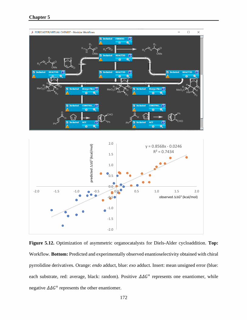
Chapter 5
172
Figure 5.12. Optimization of asymmetric organocatalysts for Diels-Alder cycloaddition. Top:
Workflow. Bottom: Predicted and experimentally observed enantioselectivity obtained with chiral
pyrrolidine derivatives. Orange: endo adduct, blue: exo adduct. Insert: mean unsigned error (blue:
each substrate, red: average, black: random). Positive 𝛥𝛥𝐺⧧ represents one enantiomer, while
negative 𝛥𝛥𝐺⧧ represents the other enantiomer.
y = 0.8568x - 0.0246R² = 0.7434
-2.0
-1.5
-1.0
-0.5
0.0
0.5
1.0
1.5
2.0
-2.0 -1.5 -1.0 -0.5 0.0 0.5 1.0 1.5 2.0
observed DDG‡ (kcal/mol)
pre
dic
ted
DD
G‡
(kca
l/m
ol)

Chapter 5
173
As seen in Figure 5.12, this virtual lead optimization had a mean unsigned error as low as
0.33 kcal/mol. The most stereoselective catalysts predicted by ACE were the best (endo) and
second best (exo) experimentally. This study was completed in just a few days on a standard
Windows PC and could be extended to hundreds of analogues.
5.4.4. Scenario #4 – Catalyst Substrate Scope.
A chemist may evaluate the potential substrate scope of a given catalyst. This last set of
calculations was done using (DHQD)2PHAL, a now commercially available catalyst for the
Sharpless asymmetric dihydroxylation of alkenes. This catalyst has been virtually (and previously
experimentally) applied to 25 substrates and compared to experimental data (Figure 5.13).
Figure 5.13. Substrate scope study with (DHQD)2PHAL. Insert: mean unsigned error (blue: each
substrate, red: average, black: random). Positive 𝛥𝛥𝐺⧧ represents (R) and (R,R) isomers, while
negative 𝛥𝛥𝐺⧧ represents the other isomers.
y = 0.8645x - 0.0948R² = 0.6104
-4.0
-3.0
-2.0
-1.0
0.0
1.0
2.0
3.0
4.0
-4.0 -3.0 -2.0 -1.0 0.0 1.0 2.0 3.0 4.0
observed DDG‡ (kcal/mol)
pre
dic
ted
DD
G‡
(kca
l/m
ol)
Chapter 5
174
Overall, this last simulation suggests that the catalyst would be highly enantioselective
(≥97%ee) on ca. 25% of the substrates and on ca. 20% it would be poorly selective (≤40%ee), in
excellent agreement with the experiments. However, we observed a poorer reproducibility for
dihydroxylation (large standard deviation over multiple runs) than with the other reactions (Figure
5.10, Table 5.1). This can be explained by the significantly larger size and flexibility of the
catalysts used in dihydroxylation (Figure 5.10) and suggests a limitation of the approach. More
time and computational resources may be required to adequately search the conformational space
of such systems. Three substrates are consistently poorly predicted (over 5 runs). One of these
failures can be attributed to the poor parameterization of sulfur-containing groups (tosylate in this
case). The other two are a cis olefin (the FF parameters were developed using a trans olefin) and
a naphthalene derivative which contributes significant π-π interactions with the catalyst.
Interestingly, the predicted average enantioselectivity varies from 67 to 76%ee over 5 runs while
it is 73.6%ee experimentally with an overall good correlation with experiments.
5.5. Reproducibility.
Because ACE relies on a stochastic method (genetic algorithm with random generation of
conformations to start from), we ran the same experiments 5 times with different seed numbers
(affecting the random number generator) to evaluate the reproducibility of the method for scenarios
#1, #3 and #4 (Table 5.1). As can be seen in Table 5.1, the accuracy on all the reaction sets is highly
reproducible. However, when looking at individual results, dihydroxylation seems to be less
reproducible likely due to the significantly large size and flexibility of the systems.

Chapter 5
175
Table 5.1. Reproducibility of ACE on scenarios #1, #3 and #4.
Entry Reaction MUE 𝜟𝜟𝑮⧧ (std dev.)
Whole seta Average individual a
1 Diels-Alder with chiral aux. 0.93 (0.00) 0.93 (0.01)
2 Aldol reaction 0.94 (0.02) 0.94 (0.07)
3 Organocatalyzed Diels Alder 0.99 (0.03) 0.99 (0.10)
4 Epoxidation 0.44 (0.02) 0.44 (0.05)
5 Dihydroxylation 1.14 (0.03) 1.14 (1.30)
6 Dihydroxylation (TSFF) 1.39 (0.15) 1.39 (1.25)
7 Et2Zn addition 0.83 (0.01) 0.83 (0.09)
8 Et2Zn addition (TSFF) 1.07 (0.05) 1.07 (0.23)
9 Hydrogenation 1.42 (0.04) 1.42 (0.21)
10 Hydrogenation (TSFF) 1.44 (0.05) 1.44 (0.25)
11 Lead optimization study 0.32 (0.01) 0.32 (0.02)
12 Substrate scope study 0.96 (0.08) 0.96 (0.62)
a Whole set: MUE is average over the whole set of catalyst/substrate systems for each seed and
average and standard deviation for these 5 overall accuracy values are measured. Average
individual: the standard deviation is computed for each catalyst/substrate systems and averaged
over the set.
5.6. Conclusions.
Our efforts to interface computational and organic chemistry have led to the creation of the
VIRTUAL CHEMIST platform, which aims to shift the paradigm of pursuing asymmetric synthesis
projects. This platform is user-friendly (designed for organic chemists) and highly customizable
through the introduction of modular workflows. The power of these modular workflows and of the

Chapter 5
176
individual programs making up the VIRTUAL CHEMIST software suite (free for academic use) has
been demonstrated through the in-depth analysis of four realistic scenarios which could comprise
various asymmetric synthesis projects. We believe that every computational approach carries its
own caveats.
Here, we acknowledge that the methodology presented requires a mechanism-based
transition state to study—much like docking potential drug molecules requires a target structure.
Additionally, the MM-based computations suffer from current FF limitations, although efforts are
ongoing to overcome this obstacle. Last, large catalytic systems provide a challenge for
conformational searching in transition state optimization and can lead to simulations trapped in
local energy minima. Notwithstanding these obstacles, we demonstrated the reliability and
accuracy of our platform, which can distinguish weak from good, and good from great asymmetric
catalysts with chemical accuracy in most cases. With this platform, chemists could now test ideas
in a matter of hours, a fraction of the time needed to synthesize and test novel catalysts. We believe
that our computational approach will lead to a more efficient catalyst discovery, as our simulated
experiments allow a broader exploration of the chemical space than experiments allow, in a shorter
amount of time. Moving forward, we hope that computational chemistry will have the same impact
on organic chemistry as NMR, MS and chromatography had at the time of their incorporation into
the chemists’ toolbox or as structure-based design software had in medicinal chemistry.

Chapter 6
177
Chapter 6 – Conclusions and Future Work
Looking back over the last 60 years of computational chemistry development, it is evident
that the current state of the field has surpassed the expectations of its pioneers. With the advent of
increased computational power for even a simple user, along with the development of highly
efficient and user-friendly computational tools, the usage of these tools within the experimental
community has become widespread. This, in turn, allows experimentalists to provide essential
feedback to the computational chemistry community, which drives the computational development
efforts forward. There is a plethora of applications of computational tools in experimental
chemistry, but, in this thesis, we have focused on nucleoside modeling, cytochrome P450
inhibition prediction and the development of a virtual asymmetric catalysis platform.
To begin with, in Chapter 1 we gave a brief overview of computational tools and their
applications in organic and medicinal chemistry. These tools range from fast and less accurate
methods such as molecular mechanics (MM) to accurate, time-consuming, and computationally
expensive quantum mechanics (QM) methods. One can also combine these two methodologies to
run QM/MM simulations or can move away from these methods to focus on machine learning
(ML) methods. We showed that MM is widely used in fields ranging from protein dynamics and
folding to docking and catalyst design while QM methods are useful in explaining reaction
mechanisms, describing chemical reactivity and predicting drug sites of metabolism (SoMs), as
well as designing catalysts. To describes events such as bond breaking/forming in enzyme
catalysis, MM and QM methods must be combined to yield accurate, cost, and time-effective
calculations (QM/MM calculations). Due to their cumbersome setup which requires expertise in
computational chemistry, QM/MM simulations are generally less accessible to medicinal
chemists, but efforts are continuously made to make these simulations more user-friendly. The last

Chapter 6
178
class of computational methods we discussed was ML, which has become widespread in
computational chemistry, and has led to some very interesting applications, particularly in
medicinal chemistry. For example, several ML tools have been proposed for predicting the SoMs
of drug-like molecules. These tools are fast and easy to use when setup in user-friendly
environments (i.e. standalone programs or webservers) but are highly dependent on the quality of
the data they have been trained on.
Following the introduction to computational tools in Chapter 1, in Chapter 2 we focused
our attention on nucleoside modeling. Generally, nucleosides preferentially adopt two different
conformations that are in equilibrium in solution: North and South, determined through the
computation of the pseudorotational phase angle P. The distinction between these conformations
is important, since nucleosides with a sugar pucker in the South conformation are preferentially
phosphorylated by kinases, while North type nucleosides are preferentially incorporated by
polymerases. To establish the North/South equilibrium, each nucleoside must be synthesized and
subjected to NMR experiments. This methodology involves significant synthetic cost, waste
production, energy expenditure, and time. To expedite the process and reduce the cost associated
with synthesizing nucleosides, we developed a medium-throughput computational protocol based
on hybrid QM/MM umbrella sampling simulations that allows the accurate determination of
North/South equilibrium in silico. This approach allows the design and North/South ratio
determination of hundreds of nucleoside analogues with the only cost being CPU time. In our
study, we observed that our approach yields accurate North/South ratios for a range of non-natural
nucleosides and low-energy structures that are comparable to crystal structures in the case of a set
of carbohydrates. However, this methodology is not without fault. For example, we discovered
that sulfur-containing nucleosides are not properly described by our simulations due to the lack of

Chapter 6
179
specific parameters for sulfur-containing rings in SCC-DFTB, the semiempirical model used for
the QM part of the simulations. Future work would thus involve the development of more accurate
parameters for heavy atoms such as sulfur. Moreover, it would be interesting to benchmark the
duration of the simulations at which a North/South equilibrium convergence arises. For now, our
simulations run for 73 ns, but this time could be shortened depending on the results of the
benchmark (in real time 1 ns of simulation takes on average 12-14 hours on 12 CPUs; however,
having supercomputers at our disposal allows us to run the simulations in parallel, which means
that all 73 ns of simulation can be run at the same time). In addition, the current methodology is
fairly involved and requires some computational expertise in setting up the simulations. Thus, it
would be essential to explore the implementation of a user-friendly way to setup the simulations
and analyze the results, which could make it highly attractive to organic and medicinal chemists.
Taking advantage of the methodology developed in Chapter 2, we decided to apply this
tool to non-natural nucleosides that exhibited valuable properties as described in Chapter 3. In this
chapter, we focused on two different situations. First, we determined the conformational
preferences of nucleosides containing various electronegative substituents at key positions on the
sugar ring. These substituents are excellent hyperconjugation acceptors and are known to modulate
the sugar conformations. Using our methodology, we demonstrated that we could obtain both
accurate North/South ratios for these nucleosides and computed low-energy structures that are
close to crystallographic ones, with heavy atom RMSDs < 1Å. Second, we explored the nature of
nucleosidic fluorine-hydrogen bonds, and we provided evidence (confirmed by experimental data)
of their existence.
Further work. From this work, we gained invaluable insight into how non-natural nucleosides
with different electronegative substituents behave in solution, which opens the possibility of

Chapter 6
180
designing novel nucleosides that make use of subtle interactions. Further work in this area is
underway. We have recently started a collaboration with Prof. Jack Szostak’s laboratory at Harvard
University in which we are using our methodology to establish the origin of RNA life. The RNA
world hypothesis proposes an early stage in the evolution of life in which RNA was responsible
for both catalysis and genetic inheritance. Before the evolution of protein enzymes, a replicase
made of RNA (ribozyme) may have catalyzed RNA synthesis. A more challenging problem is how
these ribozymes could have emerged from a non-enzymatic process of chemical RNA replication.
Currently, the chemical copying of RNA is not able to produce RNA products of the length and
complexity necessary to sustain ribozyme evolution. An essential component in this process is a
primer, which is added by an enzyme to the RNA template to be copied. Thus, we aim to study the
effect of the sugar conformation of the terminal residue of the primer on the rate of chemical RNA
copying. Moreover, we are further working on establishing a protocol for describing RNA-RNA
and DNA-RNA duplexes involving oligonucleotides comprised of non-natural nucleosides, which
would give us important information into how oligonucleotides would behave in macromolecular
complexes.
Another area of interest for organic and medicinal chemists is the xenobiotic metabolism
by Cytochrome P450 enzymes, which was discussed in Chapter 4. As part of phase 1 metabolism,
six CYP isoforms metabolize up to 90% of drugs currently on the market. Depending on the nature
of the drug, CYPs can metabolize it either to harmless or toxic metabolites. Moreover, if a patient
is concurrently taking multiple drugs metabolized by the same CYP isoform, the metabolism of
these drugs is altered, giving rise to drug-drug interactions. These drug-drug interactions can also
arise if one of the drugs metabolized by a CYP isoform is an inhibitor of that isoform. Most
commonly, inhibition by these drugs is reversible and takes place if a drug contains a basic nitrogen

Chapter 6
181
atom with an available lone pair that can coordinate to the heme iron (so-called Type II ligands).
Currently, CYP inhibition and toxicity is assessed using expensive experimental assays. To offset
this, we proposed a novel predictor comprised of QM, docking, and ML to enable the detection of
potential CYP inhibitors in silico, without the need to synthesize compounds of interest. Using
QM on a set of representative Type II ligands, we obtained QM energy profiles which we used to
develop a novel LJ(8-4) vdW potential in FITTED that could describe nitrogen-iron coordination.
Our self-docking study performed on 85 CYP crystal structures assembled from the PDB showed
that the novel potential can describe the nitrogen-iron coordination. Then, we developed an ANN
that could distinguish between inhibitors and non-inhibitors, and we determined its accuracy on a
set of five major CYPs using curated sets of compounds obtained from experimental bioassays.
While our ANN proved to be accurate for the training set, we observed that overtraining had
occurred, which affected the accuracy on the testing sets. In addition, we worked on improving
our SoM prediction tool IMPACTS, a hybrid method comprised of both QM-derived activation
energies for possible SoMs and docking. Our work focused on different areas, such as reactivity
indices for SoMs or new activation energies. In the end, it was a fast-to-compute SASA correction
for SoM accessibility that provided the best overall increase in accuracy (~5%). The work
presented in this chapter will be valuable and aid medicinal chemists in the drug design and
development process.
Future work. Efforts are ongoing in our research group to improve the CYP inhibition tool: 1) we
are extracting key interactions between isoform-specific residues and the ligands and including
them into the ANN input; 2) we are trying to balance out the sets to improve sensitivity; 3) we are
evaluating the use of multiple hidden layers as opposed to only one currently in use; 4) we are
optimizing hyperparameters such as dropout rate and conjugate gradient parameters; 5) we are

Chapter 6
182
currently testing a variety of ML methods, including SVM, and Random Forest models, to see
which one performs better in the task of predicting CYP inhibition.
In the last chapter (Chapter 5) we described a unique computational platform – VIRTUAL
CHEMIST – designed for organic chemists to undertake an asymmetric synthesis project from A-Z,
using only a few clicks. This platform was designed with the needs of experimentalists in mind,
meaning that no computational chemistry expertise is needed to use it. Moreover, we implemented
a user-friendly GUI that makes the entire process streamlined and easy to use, along with modular
workflows, which allows users to create their own customized projects. We validated VIRTUAL
CHEMIST on four different realistic scenarios. In the first scenario, we validated ACE on over 350
reactions from seven well-known reaction classes, obtaining an overall average mean unsigned
error (MUE) of ~ 1kcal/mol. Due to the inclusion of metal-catalyzed reactions in this set, as well
as the lack of parameters for metals in the MM3 FF used by ACE, we resorted to developing our
own QM program QUEMIST, which can optimize model systems involving any type of atom and
obtain customized FF parameters that can be used by ACE. In the second scenario, we determined
the recovery rate of known catalysts for the Shi Epoxidation and organocatalyzed Diels-Alder
cycloaddition reactions. Using VIRTUAL CHEMIST, we curated libraries for both reactions starting
from several hundred thousand molecules, and we seeded the libraries with known catalysts. Then
we computed the enantioselectivities with ACE and ranked the compounds in terms of their %ee,
obtaining an AUROC of 0.79 for Shi Epoxidation and 0.92 for organocatalyzed Diels-Alder
cycloaddition. In the third scenario we reproduced a study from the literature in which chiral
pyrrolidine derivatives were synthesized after the identification of a promising core scaffold. Using
VIRTUAL CHEMIST, we prepared the necessary customized workflow and assessed the derivatives
in both endo-Diels Alder and exo-Diels Alder cycloadditions, managing to find the best (endo) and

Chapter 6
183
second best (exo) analogues that had been determined experimentally. In the fourth scenario we
determined the substrate scope of (DHQD)2PHAL, a commercially available catalyst for the
Sharpless asymmetric dihydroxylation. Our predicted average enantioselectivity varied from 67-
76 %ee over 5 runs while it is 73.6 %ee experimentally, showing that our platform can be used
reliably in such a scenario.
Future work in this area is currently underway. We are set to improve the performance of our
predictive software, as well as to improve the GUI. Based on the invaluable feedback we have
received from the organic chemistry community, we are working on implementing new features
to improve the accuracy and usability of the platform and post-calculation data processing. For
example, we are working on providing users the ability to potentially obtain improved %ee’s by
running single point DFT energy calculations using QUEMIST on the lowest-energy transition states
that ACE produces and using these energies in the stereoselectivity computations. This approach
would have the added advantage of including electrons and more accurate dispersion corrections,
which play a significant role in large catalytic systems. Moreover, we are committed to providing
VIRTUAL CHEMIST users the ability to automate AUROC computations, as well as a streamlined
processing of results in the case of thousands of screened molecules.
Overall, the work presented in this thesis aims to aid organic and medicinal chemists in
their endeavours. We have made all efforts to provide detailed descriptions of the hypotheses,
study designs, results and limitations for each chapter. Moreover, we are committed to keeping all
the software we develop free for academic use, and are fully transparent in our validation studies,
with all our results being available for download.
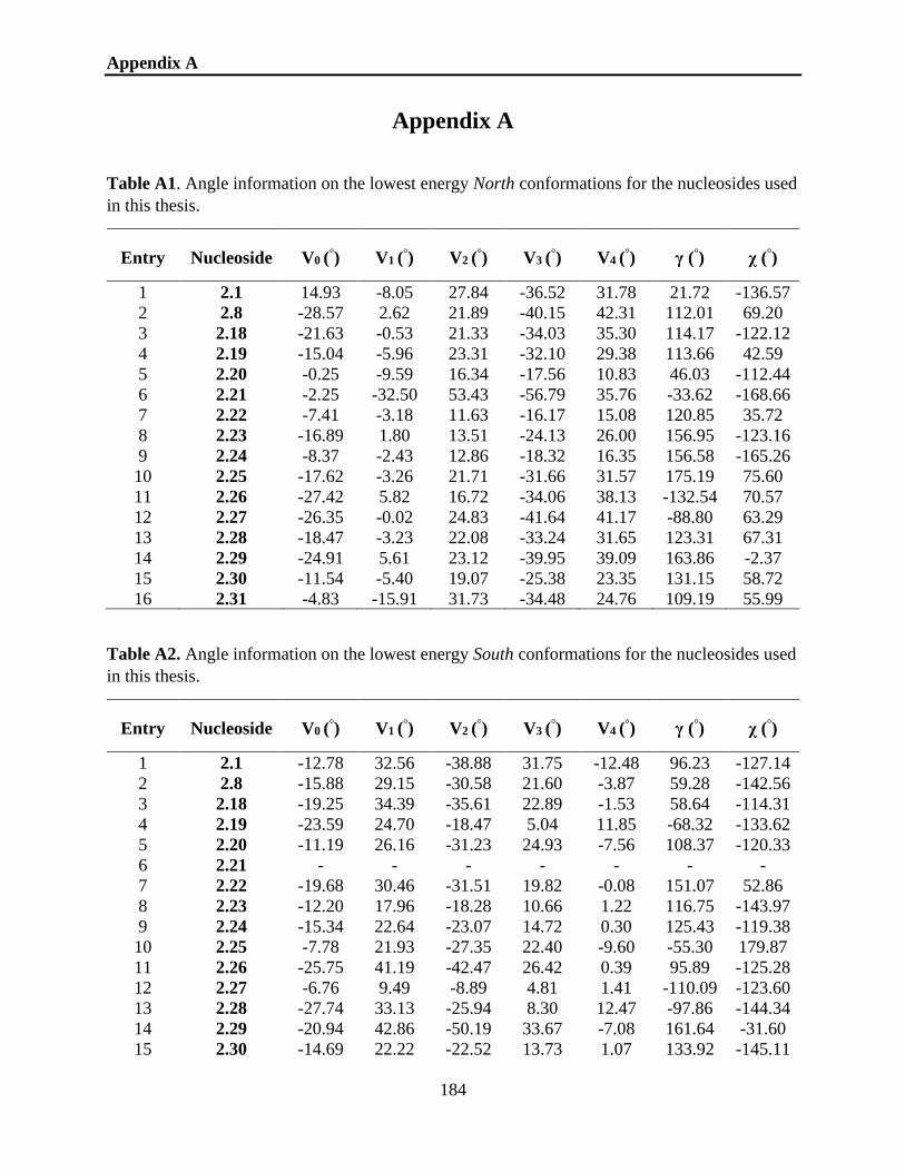
Appendix A
184
Appendix A
Table A1. Angle information on the lowest energy North conformations for the nucleosides used
in this thesis.
Entry Nucleoside V0 (°) V1 (°) V2 (°) V3 (°) V4 (°) γ (°) χ (°)
1 2.1 14.93 -8.05 27.84 -36.52 31.78 21.72 -136.57
2 2.8 -28.57 2.62 21.89 -40.15 42.31 112.01 69.20
3 2.18 -21.63 -0.53 21.33 -34.03 35.30 114.17 -122.12
4 2.19 -15.04 -5.96 23.31 -32.10 29.38 113.66 42.59
5 2.20 -0.25 -9.59 16.34 -17.56 10.83 46.03 -112.44
6 2.21 -2.25 -32.50 53.43 -56.79 35.76 -33.62 -168.66
7 2.22 -7.41 -3.18 11.63 -16.17 15.08 120.85 35.72
8 2.23 -16.89 1.80 13.51 -24.13 26.00 156.95 -123.16
9 2.24 -8.37 -2.43 12.86 -18.32 16.35 156.58 -165.26
10 2.25 -17.62 -3.26 21.71 -31.66 31.57 175.19 75.60
11 2.26 -27.42 5.82 16.72 -34.06 38.13 -132.54 70.57
12 2.27 -26.35 -0.02 24.83 -41.64 41.17 -88.80 63.29
13 2.28 -18.47 -3.23 22.08 -33.24 31.65 123.31 67.31
14 2.29 -24.91 5.61 23.12 -39.95 39.09 163.86 -2.37
15 2.30 -11.54 -5.40 19.07 -25.38 23.35 131.15 58.72
16 2.31 -4.83 -15.91 31.73 -34.48 24.76 109.19 55.99
Table A2. Angle information on the lowest energy South conformations for the nucleosides used
in this thesis.
Entry Nucleoside V0 (°) V1 (°) V2 (°) V3 (°) V4 (°) γ (°) χ (°)
1 2.1 -12.78 32.56 -38.88 31.75 -12.48 96.23 -127.14
2 2.8 -15.88 29.15 -30.58 21.60 -3.87 59.28 -142.56
3 2.18 -19.25 34.39 -35.61 22.89 -1.53 58.64 -114.31
4 2.19 -23.59 24.70 -18.47 5.04 11.85 -68.32 -133.62
5 2.20 -11.19 26.16 -31.23 24.93 -7.56 108.37 -120.33
6 2.21 - - - - - - -
7 2.22 -19.68 30.46 -31.51 19.82 -0.08 151.07 52.86
8 2.23 -12.20 17.96 -18.28 10.66 1.22 116.75 -143.97
9 2.24 -15.34 22.64 -23.07 14.72 0.30 125.43 -119.38
10 2.25 -7.78 21.93 -27.35 22.40 -9.60 -55.30 179.87
11 2.26 -25.75 41.19 -42.47 26.42 0.39 95.89 -125.28
12 2.27 -6.76 9.49 -8.89 4.81 1.41 -110.09 -123.60
13 2.28 -27.74 33.13 -25.94 8.30 12.47 -97.86 -144.34
14 2.29 -20.94 42.86 -50.19 33.67 -7.08 161.64 -31.60
15 2.30 -14.69 22.22 -22.52 13.73 1.07 133.92 -145.11

Appendix A
185
16 2.31 -9.89 26.79 -34.23 28.98 -11.62 153.75 56.80
Table A3. Puckering information obtained for the nucleosides following the umbrella sampling
simulations
*P = pseudorotational phase angle; **ϕm = puckering amplitude;
Entry Nucleoside PN* (°) ϕm**(°) PS* (°) ϕm**(°)
1 2.1 41.3 37.0 179.5 38.9
2 2.8 58.5 43.0 168.5 31.2
3 2.18 54.0 36.3 165.1 36.9
4 2.19 44.5 32.7 135.5 25.7
5 2.20 20.7 17.5 177.1 31.3
6 2.21 20.8 57.1 0.0 0.0
7 2.22 44.8 16.4 162.7 33.0
8 2.23 58.9 26.1 159.8 19.5
9 2.24 45.7 18.4 161.7 24.3
10 2.25 49.3 33.3 181.6 27.4
11 2.26 64.0 38.1 162.6 44.5
12 2.27 55.0 43.3 154.8 9.8
13 2.28 49.7 34.1 140.8 33.5
14 2.29 57.0 42.5 171.5 50.8
15 2.30 43.1 26.1 160.7 23.9
16 2.31 26.3 35.4 182.1 34.3

Appendix A
186
Table A4. Data obtained following the NBO analysis carried out at the M06L/def2-TZVP level
of theory.
Entry Nucleoside
ΔσC3’H –
σ*C4’R
(kcal/mol)
ΔσC3’H –
σ*C2’R
(kcal/mol)
ΔσC2’H –
σ*C3’R
(kcal/mol)
ΔσC3’C4’ –
σ*C2’R
(kcal/mol)
ΔσC1’2’ –
σ*C3’R
(kcal/mol)
ΔnO4’ -
σ*C4’R
(kcal/mol)
1 2.1 +1.8 +1.5 -4.7 -2.5 +1.8 +1.8
2 2.8 +2.7 +2.4 -1.8 -2.3 +0.2 +1.9
3 2.18 +5.2 +2.3 -3.4 -3.3 +2.2 +7.7
4 2.19 +2.8 -0.3 +0.3 +2.2 +1.3 +5.0
5 2.20 +2.1 +0.3 -1.6 +1.1 +1.2 +1.1
6 2.21 +2.8 +2.5 0.0 +0.1 +5.8 +7.5
7 2.22 +1.2 +0.8 +0.5 +1.2 +1.0 -0.6
8 2.23 +0.4 +0.3 -0.8 -0.3 +0.4 +3.6
9 2.24 +1.8 +0.7 -1.4 -0.6 +1.1 +2.2
10 2.25 +1.9 +2.2 -2.3 -2.1 +1.37 +1.1
11 2.26 +1.8 +3.1 -2.9 -2.3 +1.5 +1.5
12 2.27 +1.9 +2.0 -1.1 -1.0 +2.2 +1.2
13 2.28 +0.8 +0.0 +0.3 +4.0 +1.9 +0.3
14 2.29 +3.3 +1.4 +0.5 +1.8 +1.4 +2.2
15 2.30 +0.9 +0.2 +0.4 +1.7 +1.6 -0.1
16 2.31 +3.7 +0.0 -3.5 +1.3 +1.8 +0.8
The values in Table A4 are presented as energy differences of the stereoelectronic effects found in
the North and South conformation (a + value denotes a stereoelectronic effect dominant in the
North conformation, while a – value denotes a stereoelectronic effect dominant in the South
conformation).

Appendix A
187
The molecular orbitals depicting intramolecular hydrogen bonding (wireframe) for the North and
South conformations were determined using the molecular orbitals obtained following the natural
bond orbital analysis. The structures were built in Molekel, using an isosurface value of 0.01.
Figure A1. Intramolecular hydrogen bonds for the North and South puckers for 2.22. Left – North
conformation – hydrogen bond between C=O and C5’-OH. Right – South conformation –
hydrogen bonds between C5’-OH-C=O and C=O-C2’-OH.
Figure A2. Intramolecular hydrogen bonds for the North pucker for 2.25. Hydrogen bonds
between C5’-OH-O4’ and C=O-H2’ and C=O-H3’.
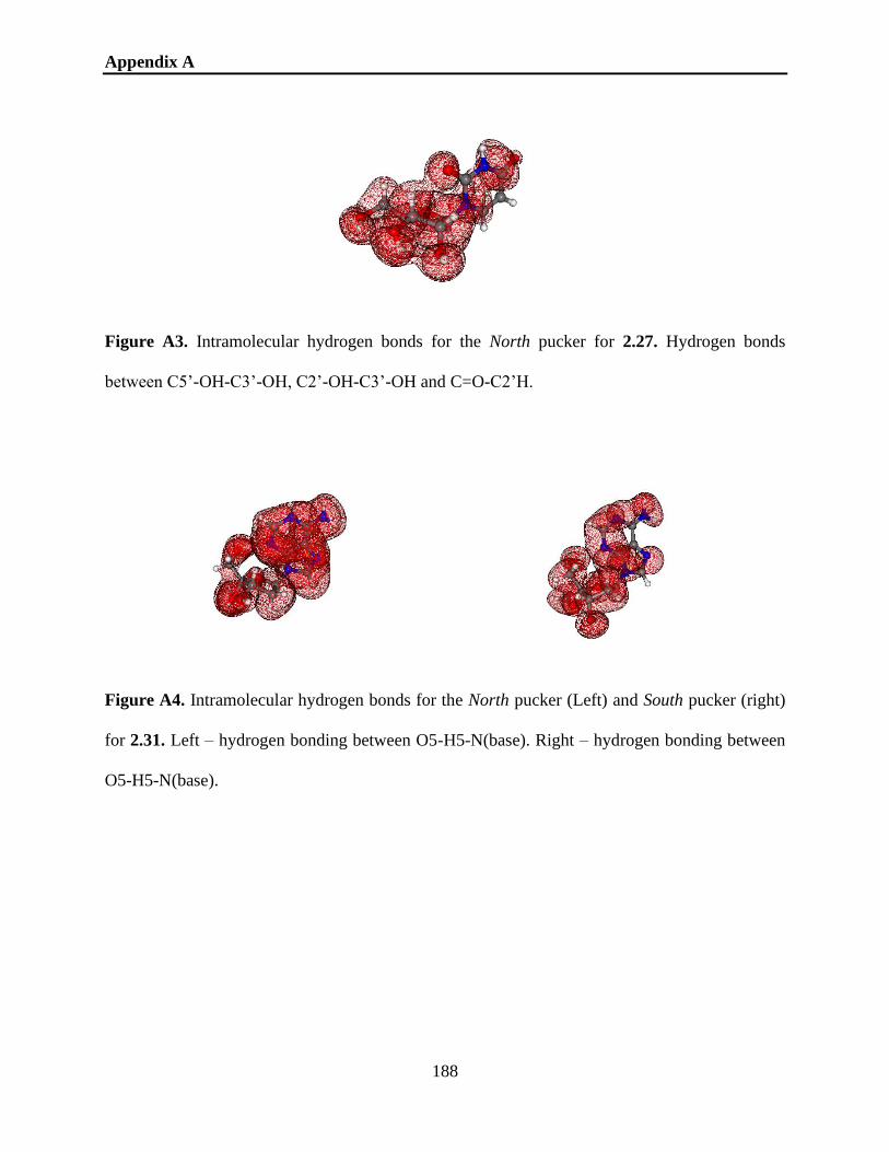
Appendix A
188
Figure A3. Intramolecular hydrogen bonds for the North pucker for 2.27. Hydrogen bonds
between C5’-OH-C3’-OH, C2’-OH-C3’-OH and C=O-C2’H.
Figure A4. Intramolecular hydrogen bonds for the North pucker (Left) and South pucker (right)
for 2.31. Left – hydrogen bonding between O5-H5-N(base). Right – hydrogen bonding between
O5-H5-N(base).

Appendix A
189
The puckering distributions and PMFs were obtained using the weighted histogram analysis
method. For an optimal resolution 73 bins were selected for constructing the graphs and curves.
Figure A5. PMF curve for 2.1 along the pseudorotational angle P. Inset shows the puckering
distribution around the same angle. Blue – Northern conformation, Green – Southern
conformation.

Appendix A
190
Figure A6. PMF curve for 2.18 along the pseudorotational angle P. Inset shows the puckering
distribution around the same angle. Blue – Northern conformation, Green – Southern
conformation.

Appendix A
191
Figure A7. PMF curve for 2.19 along the pseudorotational angle P. Inset shows the puckering
distribution around the same angle. Blue – Northern conformation, Green – Southern
conformation.

Appendix A
192
Figure A8. PMF curve for 2.20 along the pseudorotational angle P. Inset shows the puckering
distribution around the same angle. Blue – Northern conformation, Green – Southern
conformation.

Appendix A
193
Figure A9. PMF curve for 2.21 along the pseudorotational angle P. Inset shows the puckering
distribution around the same angle. Blue – Northern conformation.

Appendix A
194
Figure A10. PMF curve for 2.22 along the pseudorotational angle P. Inset shows the puckering
distribution around the same angle. Blue – Northern conformation, Green – Southern
conformation.

Appendix A
195
Figure A11. PMF curve for 2.23 along the pseudorotational angle P. Inset shows the puckering
distribution around the same angle. Blue – Northern conformation, Green – Southern
conformation.

Appendix A
196
Figure A12. PMF curve for 2.24 along the pseudorotational angle P. Inset shows the puckering
distribution around the same angle. Blue – Northern conformation, Green – Southern
conformation.

Appendix A
197
Figure A13. PMF curve for 2.25 along the pseudorotational angle P. Inset shows the puckering
distribution around the same angle. Blue – Northern conformation, Green – Southern
conformation.

Appendix A
198
Figure A14. PMF curve for 2.26 along the pseudorotational angle P. Inset shows the puckering
distribution around the same angle. Blue – Northern conformation, Green – Southern
conformation.

Appendix A
199
Figure A15. PMF curve for 2.27 along the pseudorotational angle P. Inset shows the puckering
distribution around the same angle. Blue – Northern conformation, Green – Southern
conformation.

Appendix A
200
Figure A16. PMF curve for 2.29 along the pseudorotational angle P. Inset shows the puckering
distribution around the same angle. Blue – Northern conformation, Green – Southern
conformation.
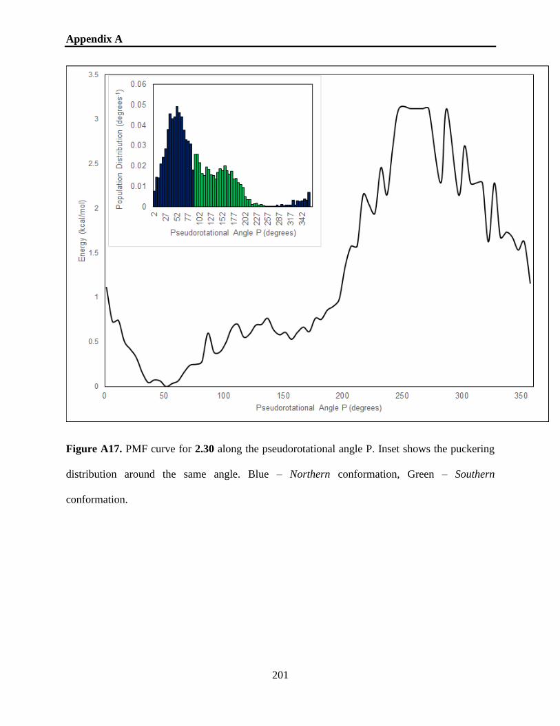
Appendix A
201
Figure A17. PMF curve for 2.30 along the pseudorotational angle P. Inset shows the puckering
distribution around the same angle. Blue – Northern conformation, Green – Southern
conformation.

Appendix A
202
Figure A18. PMF curve for 2.31 along the pseudorotational angle P. Inset shows the puckering
distribution around the same angle. Blue – Northern conformation, Green – Southern
conformation.

Appendix A
203
Figure A19. PMF curve for 2.9 along the pseudorotational angle P. Inset shows the puckering
distribution around the same angle. Blue – Northern conformation, Green – Southern
conformation.
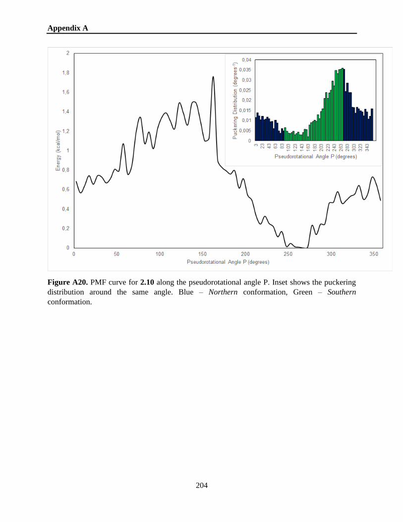
Appendix A
204
Figure A20. PMF curve for 2.10 along the pseudorotational angle P. Inset shows the puckering
distribution around the same angle. Blue – Northern conformation, Green – Southern
conformation.

Appendix A
205
Figure A21. PMF curve for 2.11 along the pseudorotational angle P. Inset shows the puckering
distribution around the same angle. Blue – Northern conformation, Green – Southern
conformation.

Appendix A
206
Figure A22. PMF curve for 2.12 along the pseudorotational angle P. Inset shows the puckering
distribution around the same angle. Blue – Northern conformation, Green – Southern
conformation.

Appendix A
207
Figure A23. PMF curve for 2.13 along the pseudorotational angle P. Inset shows the puckering
distribution around the same angle. Blue – Northern conformation, Green – Southern
conformation.

Appendix A
208
Figure A24. PMF curve for 2.14 along the pseudorotational angle P. Inset shows the puckering
distribution around the same angle. Blue – Northern conformation, Green – Southern
conformation.

Appendix A
209
Figure A25. PMF curve for 2.15 along the pseudorotational angle P. Inset shows the puckering
distribution around the same angle. Blue – Northern conformation, Green – Southern
conformation.

Appendix A
210
Figure A26. PMF curve for 2.16 along the pseudorotational angle P. Inset shows the puckering
distribution around the same angle. Blue – Northern conformation, Green – Southern
conformation.

Appendix A
211
Figure A27. PMF curve for 2.17 along the pseudorotational angle P. Inset shows the puckering
distribution around the same angle. Blue – Northern conformation, Green – Southern
conformation.

Appendix A
212
Figure A28. E4 conformer – monosaccharide 2.9.
Figure A29. 4TO conformer – monosaccharide 2.10.
Figure A30. 1T2 conformer – monosaccharide 2.11.

Appendix A
213
Figure A31. 3E conformer – monosaccharide 2.12.
Figure A32. 3T2 conformer – monosaccharide 2.13.
Figure A33. E1 conformer – monosaccharide 2.14.

Appendix A
214
Figure A34. 3T2 conformer – monosaccharide 2.15.
Figure A35. OE conformer – monosaccharide 2.16.

Appendix A
215
Figure A36. 3T4 conformer – monosaccharide 2.17.

Appendix B
216
Appendix B
Figure B1. PMF and distribution for 3.2. Experimentally determined N/S ratio is 72:28; predicted
N/S ratio is 66:34 (based on Boltzmann population distribution). Ratio by energy difference: 73:27.
Table B1. Dihedral angle data obtained for the lowest energy structures of 3.2 in Figure 3.2. The
dihedral angles are described in Chapter 2.
Conf. V0 (°) V1 (°) V2 (°) V3 (°) V4 (°) χ (°) γ (°)
North -21.39 3.03 14.74 -26.68 29.22 -147.16 -55.87
South -19.83 37.71 -40.68 27.58 -4.44 -136.14 102.10

Appendix B
217
Table B2. Hyperconjugation and anomeric effects obtained for the lowest energy structures of 3.2
in Figure 3.2. Energies given in kcal/mol. Conf. σC3’H3’ –
σ*C2’OMe
nO4’ –
σ*C4’OMe
nO4’ –
σ*C2’OMe
σ C2’H2’ –
σ*C3’OH
σ C3’H3’ –
σ*C4’OMe
σC3’C4’ –
σ*C2’OMe
σC1’C2’ –
σ*C3’OH
σ C3’H3’–
σ* C2’H2’
σ C2’H2’ –
σ* C3’H3’
North 1.95 10.47 0.06 0.74 2.15 0.54 1.34 0.71 0.93
South 0.00 9.88 0.52 3.63 0.10 4.08 0.08 0.24 0.35
Δ +1.95 +0.59 -0.46 -2.89 +2.05 -3.54 +1.26 +0.47 +0.58
Figure B2. PMF and distribution for 3.3. Experimentally determined N/S ratio is 87:13; predicted
N/S ratio is 71:29 (based on Boltzmann population distribution). Ratio by energy difference: 76:24.

Appendix B
218
Table B3. Dihedral angle data obtained for the lowest energy structures of 3.3 in Figure 3.2. The
dihedral angles are described in Chapter 2.
Conf. V0 (°) V1 (°) V2 (°) V3 (°) V4 (°) χ (°) γ (°)
North -22.81 0.08 20.38 -33.73 35.07 -130.03 10.57
South -17.84 27.09 -26.21 14.94 1.63 -129.18 -79.39
Table B4. Hyperconjugation and anomeric effects obtained for the lowest energy structures of 3.3
in Figure 3.2. Energies given in kcal/mol. Conf. σC3’H3’ –
σ*C2’OMe
nO4’ –
σ*C4’F
nO4’ –
σ*C2’OMe
σ C2’H2’ –
σ*C3’OH
σ C3’H3’ –
σ*C4’F
σC3’C4’ –
σ*C2’OMe
σC1’C2’ –
σ*C3’OH
σ C3’H3’–
σ* C2’H2’
σ C2’H2’ –
σ* C3’H3’
North 2.00 14.12 0.00 0.09 3.63 0.00 1.48 0.47 0.35
South 0.00 11.13 0.29 2.97 0.49 2.23 0.00 0.29 0.44
Δ +2.00 +2.99 -0.29 -2.88 +3.14 -2.23 +1.48 +0.18 -0.09
Figure B3. PMF and distribution for 3.8. Experimentally determined N/S ratio is 80:20; predicted
N/S ratio is 79:21 (based on Boltzmann population distribution). Ratio by energy difference: 85:15.

Appendix B
219
Table B5. Dihedral angle data obtained for the lowest energy structures of 3.8 in Figure 3.2. The
dihedral angles are described in Chapter 2.
Conf. V0 (°) V1 (°) V2 (°) V3 (°) V4 (°) χ (°) γ (°)
North -11.40 -3.17 14.98 -20.98 20.64 54.97 -34.78
South -13.92 16.47 -14.14 6.35 5.19 55.25 -139.92
Table B6. Hyperconjugation and anomeric effects obtained for the lowest energy structures of 3.8
in Figure 3.2. Energies given in kcal/mol. Conf. σC3’H3’ –
σ*C2’H2’ nO4’ –
σ*C4’OMe nO4’ –
σ*C2’H2’ σ C3’H3’ –
σ*C4’OMe σC3’C4’ –
σ*C2’H2’ σC1’C2’ –
σ*C3’OH σ C2’F – σ*
C3’H3’
North 1.10 12.60 0.00 3.23 0.22 1.40 0.11
South 0.50 12.74 0.11 1.36 0.99 0.73 0.21
Δ +0.6 -0.14 -0.11 +1.87 -0.77 +0.67 -0.10
Figure B4. Portion of the 13C spectrum of 3.10 in DMSO-d6 showing the region where the C8 and
C4 signals appear.

Appendix C
220
Appendix C
PES scans for the ligands in Chart 4.1.
Figure C1. PES Scan for ligand 4.1. Red – QM. Blue – new potential developed in FITTED.
-35
-30
-25
-20
-15
-10
-5
0
5
10
15
20
0 5 10 15
Ener
gy (
kcal
/mo
l)
Fe-N Distance (Angstrom)
DFT
LJ(8-4) + FITTED

Appendix C
221
Figure C2. PES Scan for ligand 4.2. Red – QM. Blue – new potential developed in FITTED.
Figure C3. PES Scan for ligand 4.3. Red – QM. Blue – new potential developed in FITTED.
-35
-30
-25
-20
-15
-10
-5
0
5
10
15
20
0 5 10 15
Ener
gy (
kcal
/mo
l)
Fe-N Distance (Angstrom)
QM
LJ(8-4)+MM
-40
-30
-20
-10
0
10
20
0 5 10 15
Ener
gy (
kcal
/mo
l)
Fe-N Distance (Angstrom)
QM
LJ(8-4)+MM

Appendix C
222
Figure C4. PES Scan for ligand 4.4. Red – QM. Blue – new potential developed in FITTED.
Figure C5. PES Scan for ligand 4.5. Red – QM. Blue – new potential developed in FITTED.
-35
-30
-25
-20
-15
-10
-5
0
5
10
15
20
0 5 10 15
Ener
gy (
kcal
/mo
l)
Fe-N Distance (Angstrom)
QM
LJ(8-4)+MM
-35
-30
-25
-20
-15
-10
-5
0
5
10
15
20
0 5 10 15
Ener
gy (
kcal
/mo
l)
Fe-N Distance (Angstrom)
QM
LJ(8-4) + MM

Appendix C
223
Figure C6. PES Scan for ligand 4.6. Red – QM. Blue – new potential developed in FITTED.
Figure C7. PES Scan for ligand 4.9. Red – QM. Blue – new potential developed in FITTED.
-35
-30
-25
-20
-15
-10
-5
0
5
10
15
20
0 5 10 15
Ener
gy (
kcal
/mo
l)
Fe-N Distance (Angstrom)
QM
LJ(8-4)+MM
-30
-25
-20
-15
-10
-5
0
5
10
15
20
0 5 10 15
Ener
gy (
kcal
/mo
l)
Fe-N Distance (Angstrom)
QM
LJ(8-4)+MM
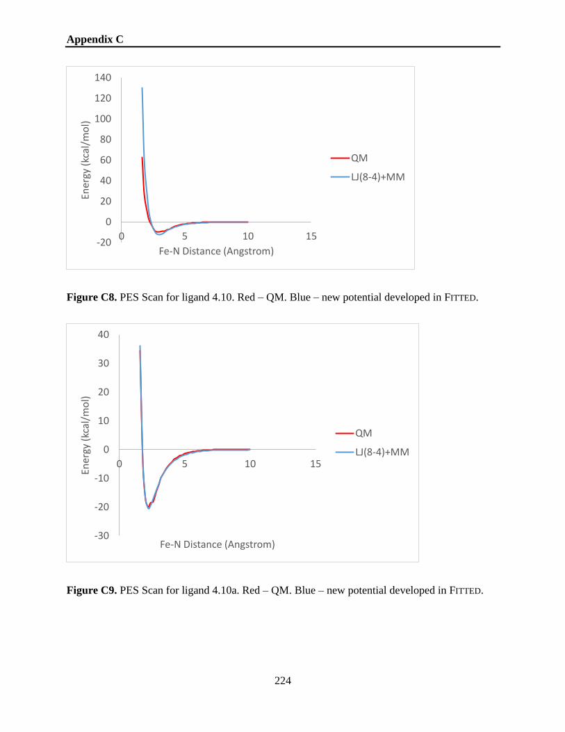
Appendix C
224
Figure C8. PES Scan for ligand 4.10. Red – QM. Blue – new potential developed in FITTED.
Figure C9. PES Scan for ligand 4.10a. Red – QM. Blue – new potential developed in FITTED.
-20
0
20
40
60
80
100
120
140
0 5 10 15
Ener
gy (
kcal
/mo
l)
Fe-N Distance (Angstrom)
QM
LJ(8-4)+MM
-30
-20
-10
0
10
20
30
40
0 5 10 15
Ener
gy (
kcal
/mo
l)
Fe-N Distance (Angstrom)
QM
LJ(8-4)+MM

Appendix C
225
Figure C10. PES Scan for ligand 4.11. Red – QM. Blue – new potential developed in FITTED.
Figure C11. PES Scan for ligand 4.12. Red – QM. Blue – new potential developed in FITTED.
-30
-20
-10
0
10
20
30
40
50
0 5 10 15Ener
gy (
kcal
/mo
l)
Fe-N Distance (Angstrom)
QM
LJ(8-4)+MM
-40
-20
0
20
40
60
80
100
0 5 10 15
Ener
gy (
kcal
/mo
l)
Fe-N Distance (Angstrom)
QM
LJ(8-4)+MM

Appendix C
226
Figure C12. PES Scan for ligand 4.13. Red – QM. Blue – new potential developed in FITTED.
Figure C13. PES Scan for ligand 4.14. Red – QM. Blue – new potential developed in FITTED.
-35
-30
-25
-20
-15
-10
-5
0
5
10
15
0 5 10 15
Ener
gy (
kcal
/mo
l)
Fe-N Distance (Angstrom)
DFT
LJ(8-4) + FITTED
-30
-25
-20
-15
-10
-5
0
5
10
15
0 5 10 15
Ener
gy (
kcal
/mo
l)
Fe-N Distance (Angstrom)
QM
LJ(8-4)+MM

Appendix C
227
Figure C14. PES Scan for ligand 4.15. Red – QM. Blue – new potential developed in FITTED.
Figure C15. PES Scan for ligand 4.16. Red – QM. Blue – new potential developed in FITTED.
-30
-25
-20
-15
-10
-5
0
5
10
15
0 5 10 15
Ener
gy (
kcal
/mo
l)
Fe-N Distance (Angstrom)
QM
LJ(8-4) + MM
-25
-20
-15
-10
-5
0
5
10
15
0 5 10 15
Ener
gy (
kcal
/mo
l)
Fe-N Distance (Angstrom)
QM
LJ(8-4) + MM

Appendix C
228
Figure C16. PES Scan for ligand 4.17. Red – QM. Blue – new potential developed in FITTED.
Figure C17. PES Scan for ligand 4.18. Red – QM. Blue – new potential developed in FITTED.
-30
-20
-10
0
10
20
30
0 5 10 15
Ener
gy (
kcal
/mo
l)
Fe-N Distance (Angstrom)
QM
-25
-20
-15
-10
-5
0
5
10
15
20
25
30
0 5 10 15
Ener
gy (
kcal
/mo
l)
Fe-N Distance (Angstrom)
QM
LJ(8-4) + MM

Appendix C
229
Figure C18. PES Scan for ligand 4.19. Red – QM. Blue – new potential developed in FITTED.
Figure C19. PES Scan for ligand 4.20. Red – QM. Blue – new potential developed in FITTED.
-30
-25
-20
-15
-10
-5
0
5
10
0 5 10 15
Ener
gy (
kcal
/mo
l)
Fe-N Distance (Angstrom)
QM
LJ(8-4) + MM
-30
-25
-20
-15
-10
-5
0
5
10
15
20
25
0 5 10 15
Ener
gy (
kcal
/mo
l)
Fe-N Distance (Angstrom)
QM
LJ(8-4) + MM
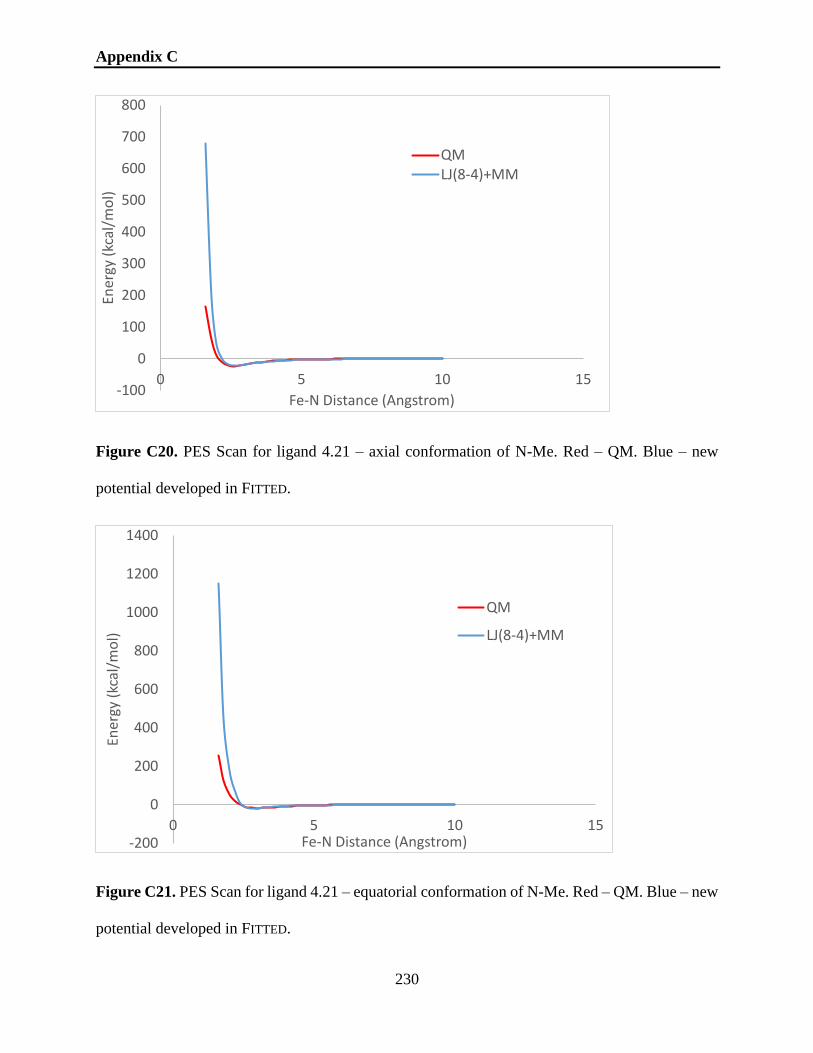
Appendix C
230
Figure C20. PES Scan for ligand 4.21 – axial conformation of N-Me. Red – QM. Blue – new
potential developed in FITTED.
Figure C21. PES Scan for ligand 4.21 – equatorial conformation of N-Me. Red – QM. Blue – new
potential developed in FITTED.
-100
0
100
200
300
400
500
600
700
800
0 5 10 15
Ener
gy (
kcal
/mo
l)
Fe-N Distance (Angstrom)
QMLJ(8-4)+MM
-200
0
200
400
600
800
1000
1200
1400
0 5 10 15
Ener
gy (
kcal
/mo
l)
Fe-N Distance (Angstrom)
QM
LJ(8-4)+MM

Appendix C
231
Figure C22. PES Scan for ligand 4.22 – axial conformation of N-Me. Red – QM. Blue – new
potential developed in FITTED.
Figure C23. PES Scan for ligand 4.22 – equatorial conformation of N-Me. Red – QM. Blue – new
potential developed in FITTED.
-200
0
200
400
600
800
1000
1200
0 5 10 15
Ener
gy (
kcal
/mo
l)
Fe-N Distance (Angstrom)
QM
LJ(8-4)+MM
-200
0
200
400
600
800
1000
1200
0 5 10 15
Ener
gy (
kcal
/mo
l)
Fe-N Distance (Angstrom)
QM
LJ(8-4)+MM

Appendix C
232
Figure C24. PES Scan for ligand 4.23 – axial conformation of N-Me. Red – QM. Blue – new
potential developed in FITTED.
Figure C25. PES Scan for ligand 4.23 – equatorial conformation of N-Me. Red – QM. Blue – new
potential developed in FITTED.
-100
0
100
200
300
400
500
600
700
800
900
0 5 10 15
Ener
gy (
kcal
/mo
l)
Fe-N Distance (Angstrom)
QM
LJ(8-4)+MM
-100
0
100
200
300
400
500
600
700
0 5 10 15
Ener
gy (
kcal
/mo
l)
Fe-N Distance (Angstrom)
QMLJ(8-4)+MM

Appendix C
233
Figure C26. PES Scan for ligand 4.24. Red – QM. Blue – new potential developed in FITTED.
Figure C27. PES Scan for ligand 4.24a. Red – QM. Blue – new potential developed in FITTED.
-30
-25
-20
-15
-10
-5
0
5
10
15
20
25
0 5 10 15
Ener
gy (
kcal
/mo
l)
Fe-N Distance (Angstrom)
QMLJ(8-4)+MM
-30
-25
-20
-15
-10
-5
0
5
10
15
20
0 5 10 15
Ener
gy (
kcal
/mo
l)
Fe-N Distance (Angstrom)
QM
LJ(8-4)+MM

Appendix C
234
Figure C28. PES Scan for ligand 4.25. Red – QM. Blue – new potential developed in FITTED.
Figure C29. PES Scan for ligand 4.26. Red – QM. Blue – new potential developed in FITTED.
-25
-20
-15
-10
-5
0
5
10
15
20
0 5 10 15
Ener
gy (
kcal
/mo
l)
Fe-N Distance (Angstrom)
QM
LJ(8-4)+MM
-25
-20
-15
-10
-5
0
5
10
15
20
0 5 10 15
Ener
gy (
kcal
/mo
l)
Fe-N Distance (Angstrom)
QM
LJ(8-4)+MM

Appendix C
235
Figure C30. PES Scan for ligand 4.27. Red – QM. Blue – new potential developed in FITTED.
Figure C31. PES Scan for ligand 4.27a. Red – QM. Blue – new potential developed in FITTED.
-30
-25
-20
-15
-10
-5
0
5
10
15
20
25
0 5 10 15
Ener
gy (
kcal
/mo
l)
Fe-N Distance (Angstrom)
QM
LJ(8-4)
-25
-20
-15
-10
-5
0
5
10
15
20
0 5 10 15
Ener
gy (
kcal
/mo
l)
Fe-N Distance (Angstrom)
QM
LJ(8-4)+MM

Appendix C
236
Figure C32. PES Scan for ligand 4.28. Red – QM. Blue – new potential developed in FITTED.
Figure C33. PES Scan for ligand 4.28a. Red – QM. Blue – new potential developed in FITTED.
-25
-20
-15
-10
-5
0
5
10
15
0 5 10 15
Ener
gy (
kcal
/mo
l)
Fe-N Distance (Angstrom)
QM
LJ(8-4)+MM
-30
-20
-10
0
10
20
30
40
50
0 5 10 15Ener
gy (
kcal
/mo
l)
Fe-N Distance (Angstrom)
QM
LJ(8-4)+MM

Appendix C
237
Figure C34. PES Scan for ligand 4.28b. Red – QM. Blue – new potential developed in FITTED.
Figure C35. PES Scan for ligand 4.29. Red – QM. Blue – new potential developed in FITTED.
-30
-20
-10
0
10
20
30
40
50
60
0 5 10 15
Ener
gy (
kcal
/mo
l)
Fe-N Distance (Angstrom)
QM
LJ(8-4)+MM
-35
-30
-25
-20
-15
-10
-5
0
5
10
15
20
0 5 10 15
Ener
gy (
kcal
/mo
l)
Fe-N Distance (Angstrom)
QM
LJ(8-4)+MM

Appendix C
238
Figure C36. PES Scan for ligand 4.31. Red – QM. Blue – new potential developed in FITTED.
Figure C37. PES Scan for ligand 4.32. Red – QM. Blue – new potential developed in FITTED.
-500
0
500
1000
1500
2000
2500
3000
0 5 10 15
Ener
gy (
kcal
/mo
l)
Fe-N Distance (Angstrom)
QM
LJ(8-4)+MM
-30
-25
-20
-15
-10
-5
0
5
10
0 5 10 15
Ener
gy (
kcal
/mo
l)
Fe-N Distance (Angstrom)
QM
LJ(8-4) + MM

Appendix C
239
Figure C38. PES Scan for ligand 4.33. Red – QM. Blue – new potential developed in FITTED.
Figure C39. PES Scan for ligand 4.34. Red – QM. Blue – new potential developed in FITTED.
-30
-25
-20
-15
-10
-5
0
5
10
15
20
0 5 10 15
Ener
gy (
kcal
/mo
l)
Fe-N Distance (Angstrom)
QM
LJ(8-4) + MM
-30
-25
-20
-15
-10
-5
0
5
10
15
20
0 2 4 6 8 10 12
Ener
gy (
kcal
/mo
l)
Fe-N Distance (Angstrom)
QM
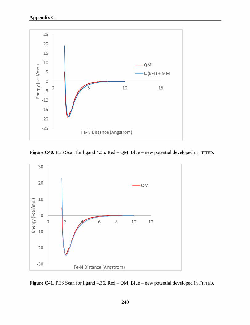
Appendix C
240
Figure C40. PES Scan for ligand 4.35. Red – QM. Blue – new potential developed in FITTED.
Figure C41. PES Scan for ligand 4.36. Red – QM. Blue – new potential developed in FITTED.
-25
-20
-15
-10
-5
0
5
10
15
20
25
0 5 10 15
Ener
gy (
kcal
/mo
l)
Fe-N Distance (Angstrom)
QM
LJ(8-4) + MM
-30
-20
-10
0
10
20
30
0 2 4 6 8 10 12
Ener
gy (
kcal
/mo
l)
Fe-N Distance (Angstrom)
QM

Appendix C
241
Figure C42. PES Scan for ligand 4.37. Red – QM. Blue – new potential developed in FITTED.
Figure C43. PES Scan for ligand 4.37a. Red – QM. Blue – new potential developed in FITTED.
-25
-20
-15
-10
-5
0
5
10
15
20
25
30
0 2 4 6 8 10 12
Ener
gy (
kcal
/mo
l)
Fe-N Distance (Angstrom)
QM
LJ(8-4) + MM
-20
-15
-10
-5
0
5
10
15
20
25
30
0 5 10 15Ener
gy (
kcal
/mo
l)
Fe-N Distance (Angstrom)
QM
LJ(8-4) + MM

Appendix C
242
Figure C44. PES Scan for ligand 4.37b. Red – QM. Blue – new potential developed in FITTED.
Figure C45. PES Scan for ligand 4.38. Red – QM. Blue – new potential developed in FITTED.
-30
-20
-10
0
10
20
30
40
50
60
0 5 10 15
Ener
gy (
kcal
/mo
l)
Fe-N Distance (Angstrom)
QM
LJ(8-4)+MM
-30
-25
-20
-15
-10
-5
0
5
10
15
20
0 5 10 15
Ener
gy (
kcal
/mo
l)
Fe-N Distance (Angstrom)
QM
LJ(8-4)+MM

Appendix C
243
Figure C46. PES Scan for ligand 4.39. Red – QM. Blue – new potential developed in FITTED.
Figure C47. PES Scan for ligand 4.40. Red – QM. Blue – new potential developed in FITTED.
-35
-30
-25
-20
-15
-10
-5
0
5
10
15
20
0 5 10 15
Ener
gy (
kcal
/mo
l)
Fe-N Distance (Angstrom)
QM
LJ(8-4)+MM
-30
-25
-20
-15
-10
-5
0
5
10
15
20
0 5 10 15
Ener
gy (
kcal
/mo
l)
Fe-N Distance (Angstrom)
QM
LJ(8-4)+MM

Appendix C
244
Table C1. Data used to build the new MM potential in FITTED (see Equation 4.1 in Chapter 4).
Inhibitor
(FITTED atom
type)
A B ε
(kcal/mol)
σ
(A) Offset
QM
Min.
(A)
MM
Min.
(A)
MAE
(kcal/mol)*
1(nb) 6066.2118 925.6305 35.31 1.6 +0.2 2.00 2.00 0.63
2(nb) 6323.9098 964.9521 36.81 1.6 +0.2 2.00 2.00 0.62
3(nb) 6607.3776 1008.2058 38.46 1.6 +0.2 2.00 2.00 0.74
4(nb) 6004.3642 916.1933 34.95 1.6 +0.2 2.00 2.00 0.54
5(nb) 6238.0105 951.8449 36.31 1.6 +0.2 2.00 2.00 0.61
6(nb) 6416.6811 979.1078 37.35 1.6 +0.2 2.00 2.00 0.63
9(n2) 5952.8246 908.3289 34.65 1.6 +0.2 2.00 2.00 0.43
10(n2) 6871.9476 1048.5760 40.00 1.6 +0.2 3.00 3.00 3.38
10a(n2) 4782.8756 729.8089 27.84 1.6 +0.2 2.20 2.20 0.33
11(n2) 5129.9089 782.7619 29.86 1.6 +0.2 2.20 2.20 0.48
12(n2) 6871.9476 1048.5760 40.00 1.6 +0.2 2.60 2.60 0.54
13(nb) 5576.5855 850.9194 32.46 1.6 +0.2 2.00 2.00 0.69
14(nb) 6012.9542 917.5040 35.00 1.6 +0.2 2.00 2.00 0.63
15(nb) 6294.7040 960.4956 36.64 1.6 +0.2 2.00 2.20 0.37
16(nb) 5463.1984 833.6179 31.80 1.6 +0.2 2.20 2.20 0.40
17(nb) 7038.5924 1074.0040 40.97 1.6 +0.2 2.20 2.40 0.88
18(nb) 5021.6757 766.2469 29.23 1.6 +0.2 2.40 2.40 0.86
19(nb) 5755.2561 878.1824 33.50 1.6 +0.2 2.20 2.20 0.49
20(nb) 5478.6603 835.9772 31.89 1.6 +0.2 2.20 2.20 0.54
21-ax(n3) 6871.9477 1048.5760 40.00 1.6 +0.2 2.60 2.60 0.42
21-eq(n3) 6871.9477 1048.5760 40.00 1.6 +0.2 3.00 3.00 0.48
22-ax(n3) 9105.3307 1389.3632 53.00 1.6 +0.2 2.60 2.60 0.77
22-eq(n3) 9105.3307 1389.3632 53.00 1.6 +0.2 3.00 3.00 0.87
23-ax(n3) 8589.9346 1310.7200 50.00 1.6 +0.2 2.60 2.60 0.62
23-eq(n3) 858.9935 131.0720 5.00 1.6 +0.2 3.00 2.80 2.20
24(n2) 5382.4530 821.2972 31.33 1.6 +0.2 2.00 2.20 0.36
24a(n2) 4781.1576 729.5468 27.83 1.6 +0.2 2.00 2.20 0.32
25(n2) 5081.8053 775.4220 29.58 1.6 +0.2 2.00 2.20 0.37
26(n2) 5056.0355 771.4898 29.43 1.6 +0.2 2.00 2.20 0.39
27(n2) 5567.9956 849.6087 32.41 1.6 +0.2 2.00 2.20 0.33
27a(n2) 3980.5757 607.3876 23.17 1.6 +0.2 2.00 2.20 0.36
28(n2) 4191.8881 639.6314 24.40 1.6 +0.2 2.00 2.00 0.35
28a(n2) 6012.6542 917.5040 35.00 1.6 +0.2 2.20 2.20 0.65
28b(n2) 4810.3633 734.0032 28.00 1.6 +0.2 2.60 2.40 0.46
29(nb) 6016.3902 918.0283 35.02 1.6 +0.2 2.00 2.00 0.50
31(n3) 6871.9477 1048.5760 40.00 1.6 +0.2 3.00 3.00 0.74
32(n2) 5239.8601 799.5392 30.50 1.6 +0.2 2.00 2.00 0.45
33(n2) 5325.7594 812.6464 31.00 1.6 +0.2 2.00 2.20 0.62
34(n2) 6098.8535 930.6112 35.50 1.6 +0.2 2.00 2.00 0.58
35(n2) 4552.6653 694.6816 26.50 1.6 +0.2 2.00 2.20 0.85
36(n2) 5669.3568 865.0752 33.00 1.6 +0.2 2.00 2.20 0.85
37(n2) 3951.3699 602.9312 23.00 1.6 +0.2 2.00 2.20 0.85

Appendix C
245
37a(n2) 4123.1686 629.1456 24.00 1.6 +0.2 2.20 2.20 0.95
37b(n2) 4466.7660 681.5744 26.00 1.6 +0.2 2.20 2.20 0.75
38(nb) 5904.7210 900.9889 34.37 1.6 +0.2 2.00 2.00 0.45
39(nb) 5995.7743 914.8826 34.90 1.6 +0.2 2.00 2.00 0.49
40(nb) 5995.7743 914.8826 34.90 1.6 +0.2 2.00 2.00 0.38
Table C2. Set used for self-docking along with docking results for both docking modes.
Entry Protein Resolution CYP
Isoform
Fe-
Coordination
Nitrogen
Hybridization
Reference
Ligands
RMSD
(Protein)
RMSD
(Metalloprotein)
1 1e9x 2.1 51 yes sp2 1 0.554 0.55
2 1ea1 2.21 51 yes sp2 1 0.43 0.376
3 1nr6 2.1 2C5 no x 1 0.498 0.545
4 1pha 1.63 CAM yes sp2 1 2.303 2.326
5 1r9o 2 2C9 no x 1 1.237 0.269
6 1z11 2.05 2A6 no x 1 0.299 0.303
7 2bdm 2.3 2B4 yes sp2 1 1.025 1.006
8 2fdw 2.05 2A6 yes sp3 1 5.464 5.453
9 2nnj 2.28 2C8 no x 1 4.629 4.653
10 2p85 2.35 2A13 no x 2 1.006 2.615
11 3czh 2.3 2R1 no x 1 0.54 9.449
12 3e6i 2.2 2E1 yes sp2 1 0.134 0.172
13 3ebs 2.15 2A6 no x 1 1.526 1.681
14 3ibd 2 2B6 yes sp2 1 0.257 1.401
15 3mdr 2 46A1 yes sp3 1 0.742 0.934
16 3mdt 2.3 46A1 yes sp2 1 0.604 2.449
17 3mdv 2.4 46A1 yes sp2 1 0.723 0.744
18 3n9y 2.1 11A1 no x 1 0.859 0.859
19 3n9z 2.17 11A1 no x 1 0.44 0.431
20 3na1 2.25 11A1 no x 1 0.527 0.354
21 3nxu 2 3A4 yes sp2 1 4.469 3.937
22 3qoa 2.1 2B6 yes sp2 1 1.858 1.65
23 3r9c 2.14 164A2 yes sp2 2 1.08 0.879
24 3swz 2.4 17A1 yes sp2 1 0.412 0.297
25 3t3q 2.1 2A6 yes sp2 1 0.337 0.383
26 3t3r 2.4 2A6 yes sp2 1 0.373 0.317
27 3t3z 2.35 2E1 yes sp2 1 0.482 0.483
28 3tbg 2.1 2D6 yes sp2 2 0.686 0.477
29 3tjs 2.25 3A4 yes sp3 1 8.222 7.606
30 3ua1 2.15 3A4 no x 1 0.774 0.548
31 4d75 2.25 3A4 yes sp2 1 3.117 4.168
32 4dvq 2.49 11B2 no x 1 0.529 0.526
33 4ejh 2.35 2A13 no x 1 5.572 5.471
34 4eji 2.1 2A13 yes sp2 2 6.304 0.687

Appendix C
246
35 4ejj 2.3 2A6 no x 1 4.473 4.462
36 4fia 2.1 46A1 yes sp 1 2.506 3.013
37 4i91 2 2B6 no x 1 2.659 2.63
38 4k9w 2.4 3A4 yes sp2 1 8.177 3.617
39 4key 2.05 BM3 no x 1 0.467 0.484
40 4kpa 2 BM3 no x 1 1.17 0.934
41 4nz2 2.45 2C9 no x 1 0.582 1.795
42 4rql 2.1 2B6 no x 1 3.595 1.54
43 4rrt 2.2 2B6 no x 1 3.499 3.501
44 4tt5 2.18 119 yes sp2 1 0.526 0.479
45 4uhi 2.05 51 yes sp2 1 0.544 0.884
46 4wmz 2.05 51 yes sp2 1 0.404 0.447
47 4wnu 2.26 2D6 no x 1 0.397 0.448
48 4wnv 2.35 2D6 no x 1 6.194 2.236
49 4wpd 2 119 yes sp2 1 0.515 0.502
50 4xrz 2.4 2D6 yes sp2 1 0.366 0.367
51 4zdz 2.3 51 yes sp2 1 1.379 1.389
52 4ze0 2.2 51 yes sp2 1 1.389 1.387
53 4ze3 2.2 51 yes sp2 1 1.213 1.757
54 4zv8 2.24 2B6 no x 1 2.857 2.862
55 5a1r 2.45 3A4 no x 1 3.756 3.558
56 5a5i 2 2C9 no x 1 1.978 2.292
57 5e58 2.4 2B35 yes sp2 2 1.481 1.542
58 5ese 2.2 51 yes sp2 1 0.715 0.692
59 5esf 2.25 51 yes sp2 1 0.798 0.697
60 5esh 2.15 51 yes sp2 1 1.185 1.355
61 5hs1 2.1 51 yes sp2 1 1.397 1.376
62 5irq 2.2 17A1 yes sp2 1 1.513 1.44
63 5k7k 2.3 2C9 yes sp2 1 2.444 2.556
64 5l92 2.1 109E1 no x 1 1.045 1.033
65 5l94 2.25 109E1 no x 1 6.342 6.299
66 5tz1 2 51 yes sp2 1 1.202 0.92
67 5uap 2.24 2B6 no x 2 0.597 0.526
68 5uec 2.27 2B6 no x 2 3.619 3.682
69 5uys 2.39 17A1 yes sp2 1 0.484 0.368
70 5vce 2.2 3A4 yes sp2 1 6.037 4.226
71 5vcg 2.2 3A4 no x 1 1.045 0.964
72 5w0c 2 2C9 no x 1 2.493 2.706
73 5x23 2 2C9 no x 1 4.716 4.664
74 5x24 2.48 2C9 no x 1 3.32 3.509
75 5xxi 2.3 2C9 no x 1 3.272 3.207
76 6a16 2 90B1 yes sp2 1 1.022 0.299
77 6a17 2.3 90B1 yes sp2 1 0.294 0.287
78 6bcz 2.23 3A4 yes sp2 1 2.086 3.104
79 6bd7 2.42 3A4 yes sp2 1 2.536 5.327

Appendix C
247
80 6bd8 2.38 3A4 yes sp2 1 6.084 3.13
81 6bdh 2.25 3A4 yes sp2 1 4.855 4.505
82 6f85 2.05 260A1 yes sp2 1 4.676 4.641
83 6jo1 2.1 102A1 no x 1 0.713 0.838
84 6m7x 2.1 11B1 yes sp2 1 0.484 0.556
85 6ung 2.3 3A4 yes sp2 1 8.103 7.615
Rigid Docking.
Table C3. Accuracy of Impacts 2019 over 5 runs using all activation energies.
Isoform Run 1 Run 2 Run 3 Run 4 Run 5 Overall
Accuracy
Std.
Dev.
1A2 77.4 77.4 77.4 73.7 74.5 76.1 1.6
2C9 76.0 80.6 79.8 80.6 78.3 79.1 1.7
2D6 70.1 74.5 73.9 71.3 75.2 73.0 2.0
3A4 74.7 74.7 74.4 73.7 73.7 74.2 0.5
Table C4. Accuracy of Impacts 2019 over 5 runs using the top 5 activation energies.
Isoform Run 1 Run 2 Run 3 Run 4 Run 5 Overall
Accuracy
Std.
Dev.
1A2 77.4 78.1 77.4 74.5 78.1 77.1 1.3
2C9 76.0 79.1 78.3 79.1 76.7 77.8 1.3
2D6 70.1 72.0 71.3 70.1 72.0 71.1 0.9
3A4 72.7 72.4 70.3 71.0 72.0 71.7 0.9
Table C5. Accuracy of Impacts 2019 over 5 runs using all activation energies and FCs.
Isoform Run 1 Run 2 Run 3 Run 4 Run 5 Overall
Accuracy
Std.
Dev.
1A2 73.0 72.3 70.8 75.9 72.3 72.8 1.7
2C9 70.5 72.9 70.5 73.6 73.6 72.2 1.4
2D6 63.1 68.2 61.1 61.1 63.1 63.3 2.6
3A4 67.2 67.6 66.9 68.6 67.2 67.5 0.6
Table C6. Accuracy of Impacts 2019 over 5 runs using the top 5 activation energies and FCs.
Isoform Run 1 Run 2 Run 3 Run 4 Run 5 Overall
Accuracy
Std.
Dev.
1A2 73.7 74.5 70.1 71.5 70.8 72.1 1.7
2C9 74.4 72.1 70.5 73.6 72.1 72.5 1.4
2D6 56.1 56.1 56.7 58.6 58.0 57.1 1.0

Appendix C
248
3A4 67.2 66.2 67.2 68.6 70.6 68.0 1.5
Table C7. Accuracy of Impacts 2019 over 5 runs using all activation energies and SASA
correction.
Isoform Run 1 Run 2 Run 3 Run 4 Run 5 Overall
Accuracy
Std.
Dev.
1A2 81.0 83.9 81.8 81.0 79.6 81.5 1.4
2C9 81.4 84.5 82.2 84.5 85.3 83.6 1.5
2D6 77.1 77.7 75.8 77.1 76.4 76.8 0.7
3A4 75.4 75.4 72.2 74.4 75.8 74.6 1.3
Table C8. Accuracy of Impacts 2019 over 5 runs using the top 5 activation energies and SASA
correction.
Isoform Run 1 Run 2 Run 3 Run 4 Run 5 Overall
Accuracy
Std.
Dev.
1A2 82.5 83.2 84.7 86.1 83.2 83.9 1.3
2C9 84.5 86.8 83.7 86.0 83.7 84.9 1.3
2D6 75.2 76.8 75.2 75.8 74.5 75.5 0.8
3A4 76.8 75.4 76.1 77.1 77.5 76.6 0.7
Table C9. Accuracy of Impacts 2019 over 5 runs using all activation energies, SASA correction
and FCs.
Isoform Run 1 Run 2 Run 3 Run 4 Run 5 Overall
Accuracy
Std.
Dev.
1A2 78.8 78.1 77.4 77.4 78.1 78.0 0.5
2C9 75.2 79.8 76.0 76.7 76.0 76.7 1.6
2D6 74.5 73.9 74.5 77.1 75.2 75.0 1.1
3A4 67.2 70.3 70.0 70.4 67.9 69.2 1.3
Table C10. Accuracy of Impacts 2019 over 5 runs using the top 5 activation energies, SASA
correction and FCs.
Isoform Run 1 Run 2 Run 3 Run 4 Run 5 Overall
Accuracy
Std.
Dev.
1A2 81.0 81.0 81.8 81.0 80.3 81.0 0.5
2C9 79.1 80.6 80.6 79.8 80.6 80.1 0.6
2D6 70.1 68.8 70.7 69.4 70.1 69.8 0.7
3A4 71.3 71.7 71.7 72.0 72.0 71.7 0.4

Appendix C
249
Table C11. Accuracy of Impacts 2019 over 5 runs using all activation energies.
Isoform Run 1 Run 2 Run 3 Run 4 Run 5 Overall
Accuracy
Std.
Dev.
1A2 66.4 68.6 69.3 68.6 65.0 67.6 1.6
2C9 70.5 69.0 67.3 67.4 69.8 68.8 1.3
2D6 47.1 48.4 49.7 45.9 51.0 48.4 1.8
3A4 67.2 67.2 65.9 66.9 66.2 66.7 0.5
Table C12. Accuracy of Impacts 2019 over 5 runs using the top 5 activation energies.
Isoform Run 1 Run 2 Run 3 Run 4 Run 5 Overall
Accuracy
Std.
Dev.
1A2 63.5 63.5 65.0 63.5 63.5 63.8 0.6
2C9 64.3 65.1 65.1 65.1 66.7 65.3 0.8
2D6 43.3 43.3 42.7 42.7 43.3 43.1 0.3
3A4 63.1 63.1 64.8 62.8 64.2 63.6 0.8
Table C13. Accuracy of Impacts 2019 over 5 runs using all activation energies.
Isoform Run 1 Run
2 Run 3 Run 4 Run 5
Overall
Accuracy
Std.
Dev.
1A2 (270) 78.1 79.6 80.0 79.6 78.1 79.1 0.8
2C9 (225) 72.0 73.3 74.7 75.1 73.3 73.7 1.1
2C19 (218) 69.7 69.7 70.6 70.6 71.1 70.3 0.6
2D6 (270) 70.4 68.5 70.7 67.7 68.5 69.2 1.2
2E1 (142) 65.7 66.9 70.4 66.2 66.9 67.2 1.7
Total molecules: 1125
Table C14. Accuracy of Impacts 2019 over 5 runs using the top 5 activation energies.
Isoform Run 1 Run 2 Run 3 Run 4 Run 5 Overall
Accuracy
Std.
Dev.
1A2 81.1 80.7 80.0 80.6 80.4 80.6 0.4
2C9 71.6 72.4 74.2 74.2 71.1 72.7 1.3
2C19 70.6 72.9 72.9 69.3 70.6 71.3 1.4
2D6 70.4 69.6 70.0 69.3 69.3 69.7 0.4
2E1 67.6 68.3 68.3 70.0 68.3 68.5 0.8

Appendix C
250
Table C15. Accuracy of Impacts 2019 over 5 runs using all activation energies and SASA
correction.
Isoform Run 1 Run 2 Run 3 Run 4 Run 5 Overall
Accuracy
Std.
Dev.
1A2 80.7 78.1 80.4 81.1 80.4 80.1 1.1
2C9 73.3 76.0 74.6 73.8 73.8 74.3 0.9
2C19 76.1 75.7 75.7 77.1 76.6 76.2 0.5
2D6 75.5 74.4 77.4 77.0 74.8 75.8 1.2
2E1 70.0 70.4 70.4 72.5 70.4 70.7 0.9
Table C16. Accuracy of Impacts 2019 over 5 runs using the top 5 activation energies and SASA
correction.
Isoform Run 1 Run 2 Run 3 Run 4 Run 5 Overall
Accuracy
Std.
Dev.
1A2 80.4 81.9 81.9 80.7 80.7 81.1 0.6
2C9 75.1 72.4 74.2 74.2 75.1 74.2 1.0
2C19 75.7 74.8 73.9 76.6 76.6 75.5 1.0
2D6 73.3 73.7 73.0 72.2 73.0 73.0 0.5
2E1 67.6 72.5 69.0 72.5 73.2 71.0 2.2
Flexible Docking.
To run flexible docking one must ensure that the population size used for selecting suitable
individuals for docking is large enough. As such, the population size used for flexible docking is
increased to 200 (in comparison to rigid docking – 100) and the maximum number of generations
is increased to 100 (in comparison to rigid docking – 50).
Table C17. Accuracy of Impacts 2019 over 5 runs using the top 5 activation energies, SASA
correction and flexible docking – initial sets.
Isoform Run 1 Run 2 Run 3 Run 4 Run 5 Overall
Accuracy
Std.
Dev.
1A2a 82.5 83.2 84.7 86.1 83.2 83.9 1.3
2C9b 77.5 76.7 77.5 76.7 77.5 77.2 0.4
2C9c 76.7 76.7 76.7 74.4 76.7 76.2 0.9
2D6d 72.6 75.2 75.8 76.4 73.9 74.8 1.4
2D6e 75.2 73.2 74.5 75.2 73.9 74.4 0.8
3A4 74.7 76.1 76.1 75.4 74.1 75.3 0.8

Appendix C
251
a results from rigid docking, isoform does not have multiple crystal structures to allow flexible
docking
b results obtained using 5 crystal structures: 1R9O, 5K7K, 5XXI, 4NZ2, 5A5J
c results obtained using 3 crystal structures: 1R9O, 5K7K, 5XXI
d results obtained using 5 crystal structures: 3QM4, 3TBG, 4WNU, 5TFT, 2F9Q
e results obtained using 3 crystal structures: 3QM4, 3TBG, 4WNU
Table C18. Accuracy of Impacts 2019 over 5 runs using the top 5 activation energies, SASA
correction and flexible docking – external sets.
Isoform Run 1 Run 2 Run 3 Run 4 Run 5 Overall
Accuracy
Std.
Dev.
1A2a 80.4 81.9 81.9 80.7 80.7 81.1 0.6
2C9b 72.7 71.8 71.8 71.8 71.8 72.0 0.4
2C9c 72.9 71.6 72.0 71.1 70.7 71.7 0.8
2C19a 75.7 74.8 73.9 76.6 76.6 75.5 1.0
2D6d 74.1 74.4 75.9 74.8 74.8 74.8 0.6
2D6e 74.1 75.2 74.4 75.2 74.4 74.7 0.5
2E1 72.5 73.9 71.1 73.2 71.8 72.5 1.0 a results from rigid docking, isoform does not have multiple crystal structures to allow flexible
docking
b results obtained using 5 crystal structures: 1R9O, 5K7K, 5XXI, 4NZ2, 5A5J
c results obtained using 3 crystal structures: 1R9O, 5K7K, 5XXI
d results obtained using 5 crystal structures: 3QM4, 3TBG, 4WNU, 5TFT, 2F9Q
e results obtained using 3 crystal structures: 3QM4, 3TBG, 4WNU

Appendix C
252
Flexible Docking – PDB Codes.
Flexible docking requires several crystal structures to ensure mutations across isoforms
and active sites, with the aim of accurate docking. To this end we have assembled several PDB
files/isoform (where available). The crystal structure PDB codes are given below:
CYP1A2
• 2HI4 (original, used in rigid docking) – 1.95Å resolution
• N/A – no other crystal structures are available for this isoform
CYP2C9
• 1R9O (original, used in rigid docking) – 2.00Å resolution
• 4NZ2 – 2.45Å resolution
• 5A5J – 2.90Å resolution
• 5K7K – 2.30Å resolution
• 5XXI – 2.30Å resolution
CYP2C19
• 4GQS (original, used in rigid docking) – 2.87Å resolution
• N/A – no other crystal structures are available for this isoform
CYP2D6
• 3QM4 (original, used in rigid docking) – 2.85Å resolution
• 3TBG – 2.10Å resolution

Appendix C
253
• 4WNU – 2.26Å resolution
• 5TFT – 2.71Å resolution
• 2F9Q – 3.00Å resolution
CYP3A4
• 3NXU (original, used in rigid docking) – 2.00Å resolution
• 1W0E – 2.80Å resolution
• 2J0D – 2.75Å resolution
• 4D78 – 2.80Å resolution
• 5TE8 – 2.70Å resolution
CYP2E1
• 3E6I (original, used in rigid docking) – 2.20Å resolution
• 3T3Z – 2.35Å resolution
• 3GPH – 2.70Å resolution
• 3E4E – 2.60Å resolution

Appendix D
254
Appendix D
All ACE and CONSTRUCTS calculations were performed with subversion 5679 of the
ACE/FORECASTER platforms. The Windows/Linux/MacOS subversion can be requested from
Nicolas Moitessier: [email protected].
Single point energy calculation using QUEMIST within the HF framework– pseudocode:
void function quemist – single point energy calculation {
set molecule and determine number of alpha and beta electrons
initialize LIBINT variables (if Linux/MacOS versions used)
create basis set as per user instructions
compute overlap integral matrix - S
compute kinetic integral matrix - T
compute nuclear attraction integral matrix - V
compute Hamiltonian = T + V
orthogonalize basis set using canonical orthogonalization {
compute eigenvectors and eigenvalues of overlap matrix S
define diagonal ortho matrix = eigenvalues of S on the principal diagonal
for (i = 0 to number of basis functions) {
if (absolute value of ortho(i,i) less than 1e-08) {
ortho(i, i) = 0.0
}
else {
ortho(i, i) = 1.0 / square root of ortho(i, i)
}
}
define unitary matrix U = eigenvectors of S
calculate the transformation matrix:
X = U * ortho
calculate the transpose of the transformation matrix:
Xp = XT
}
compute initial guess density matrix using the superposition of atomic densities in the minimal
basis STO-3G
project orbitals in actual basis set and obtain true guess density matrix
compute Schwarz boundaries for performing the Cauchy-Schwarz inequality when
computing electron repulsion integrals
initialize DIIS
for (iteration = 0 to max number of iterations requested by the user)
{
initialize Fock matrix F = Hamiltonian

Appendix D
255
compute 2e integrals and the Coulomb (J) and exchange matrices (K) and add them
to F:
F = F + J - 0.5 * K
compute electronic energy of the iteration
add nuclear repulsion energy to the electronic energy
obtain the difference in energy between iterations by subtracting the previous
iteration energy from the current iteration energy
obtain DIIS error matrix
if (iteration larger than 2) {
extrapolate Fock matrix using DIIS
}
diagonalize the Xp * F * X matrix
obtain orbital matrix C = X * (eigenvectors of Xp * F * X matrix)
obtain orbital energy matrix orbenergy = eigenvalues of the Xp * F * X matrix
check if orbitals are orthonormal
obtain new density matrix using the occupied orbitals from the orbital matrix C
obtain convergence density matrix as the difference between the new density matrix
and the previous density matrix
compute rms and maximum absolute error of the convergence density matrix
assign current energy to the last energy variable
if (difference in energy less than energy threshold OR rms less than density
threshold OR maximum absolute error less than density threshold OR DIIS error less than DIIS
threshold) {
convergence flag is true
failure flag is false
}
if (convergence flag is true) {
save current energy
save current orbitals
save current rms
save current maximum absolute error in the density matrix
save current DIIS error
exit for loop
}
else {
if (iteration less than 2) {
Current density matrix = (1 – damping factor) * new density matrix
+ damping factor * current density matrix;
}
else {
Current density matrix = new density matrix
}
}

Appendix D
256
if (reach maximum iterations AND convergence flag is false) {
failure flag is true
print failure message
}
}
If (failure flag is false)
{
print convergence details
print orbitals and orbital energies
print details of the convergence iteration
print Mulliken population analysis
print Mayer Bond Order Analysis
print Mayer Free Valence Electrons
}
}
Geometry optimization / Hessian calculation using QUEMIST and generation of FF
parameters – pseudocode:
void function quemist – geometry optimization {
set molecule and determine number of alpha and beta electrons
initialize basis set
determine redundant internal coordinates
determine degrees of freedom
determine energy at initial point (see void quemist – single point energy)
save xyz coordinates from the initial energy evaluation to coordinate file
initialize trust radius to 0.5
for (i = 0 to max number of geometry optimization steps requested by user)
{
run single point energy of the coordinates at iteration i
compute gradient (g) of coordinates at iteration i
save gradient of the iteration in gradient vector
determine norm of the gradient
if (i equals 0) {
initialize initial Hessian with the unit matrix
diagonalize initial Hessian to obtain eigenvalues
check if Hessian is positive definite based on eigenvalue values
obtain augmented Hessian (aug.Hessian) using the gradient and initial
Hessian
diagonalize augmented Hessian
obtain minimum value (mvaug) in augmented Hessian
obtain new search direction (sd) = - inverse of (aug.Hessian - mvaug *
identity matrix) * gradient
save new sd in sd vector

Appendix D
257
if (norm of sd > trust radius) {
scale sd components so that the norm of the sd is equal to the trust
radius
}
else {
accept norm of the sd as the length of the step
}
obtain new coordinates (nc) = coords. at initial point + sd
save current hessian in hessian vector
}
else {
update hessian at current iteration using the information from the hessian,
gradient, and sd from the previous iteration (BFGS formula)
diagonalize hess to obtain eigenvalues
check if Hessian is positive definite based on eigenvalue values
obtain augmented Hessian (aug.Hessian) using the gradient and initial
Hessian
diagonalize augmented Hessian
obtain minimum value (mvaug) in augmented Hessian
obtain new sd = - inverse of (aug.Hessian - mvaug * identity matrix) *
gradient
save new sd in sd vector
if (norm of sd > trust radius) {
scale sd components so that the norm of the sd is equal to the trust
radius
}
else {
accept norm of the sd as the length of the step
}
obtain new coordinates (nc) = coords. at initial point + sd
save current hessian in hessian vector
}
obtain max. error (fmax) and max rms (frms) in gradient
obtain max. error (dmax) and max rms (drms) in atomic displacements
check if thresholds have been met:
• If energy difference between iterations is < 0.0005
• If fmax < 0.0003
• If frms < 0.0001
• If dmax < 0.0020
• If drms < 0.0040
if (4 of 5 conditions are met) {
signal convergence
print orbital data, Mulliken Population Analysis and Mayer Bond Order
data
} else {
continue optimization until convergence is reached

Appendix D
258
save coordinates at this step in xyz file
if (convergence is reached and Hessian flag computation has been found) {
compute true Hessian numerically by using finite differences and a
step increment of 0.005
if (Hessian contains negative eigenvalues) {
print warning message that the geometry is not minimum
}
compute the force field parameters using the Hessian matrix and
Seminario algorithm
create parameter file named
molfilename_customized_ff_parameters.txt
}
}
}
}
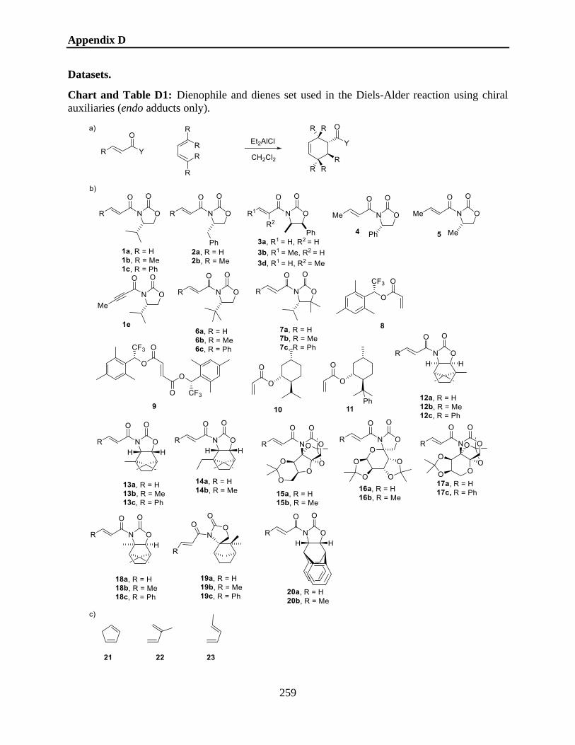
Appendix D
259
Datasets.
Chart and Table D1: Dienophile and dienes set used in the Diels-Alder reaction using chiral
auxiliaries (endo adducts only).
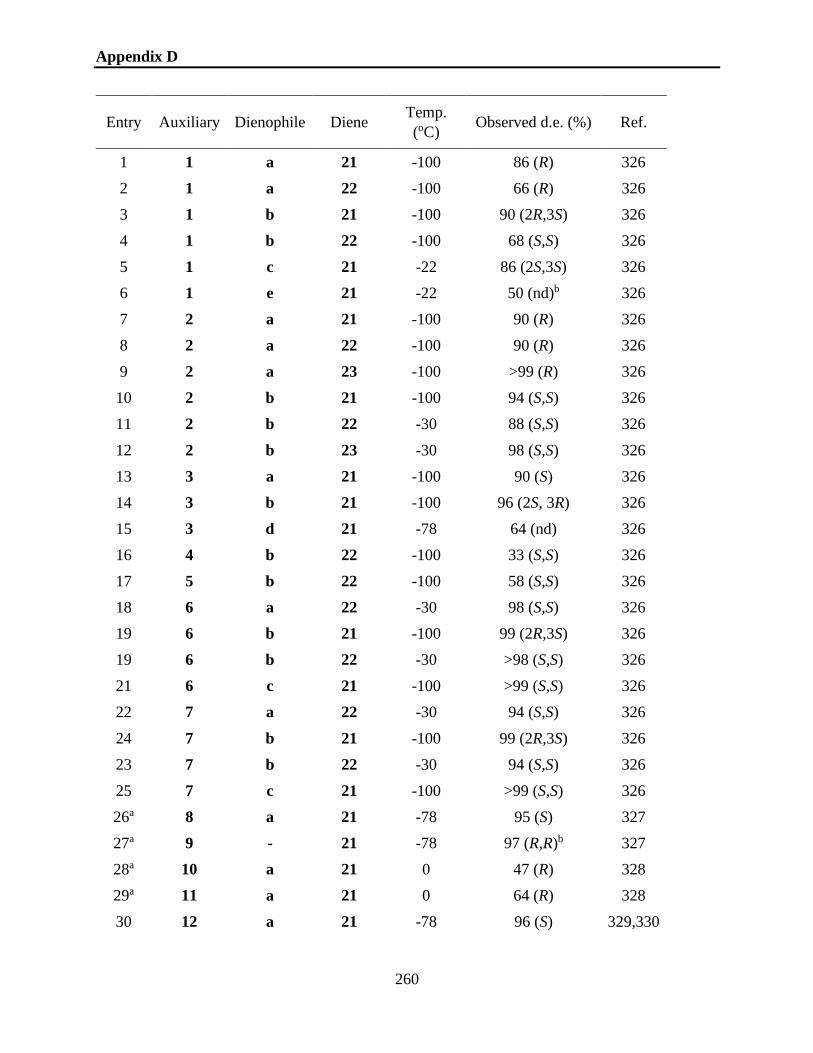
Appendix D
260
Entry Auxiliary Dienophile Diene Temp.
(oC) Observed d.e. (%) Ref.
1 1 a 21 -100 86 (R) 326
2 1 a 22 -100 66 (R) 326
3 1 b 21 -100 90 (2R,3S) 326
4 1 b 22 -100 68 (S,S) 326
5 1 c 21 -22 86 (2S,3S) 326
6 1 e 21 -22 50 (nd)b 326
7 2 a 21 -100 90 (R) 326
8 2 a 22 -100 90 (R) 326
9 2 a 23 -100 >99 (R) 326
10 2 b 21 -100 94 (S,S) 326
11 2 b 22 -30 88 (S,S) 326
12 2 b 23 -30 98 (S,S) 326
13 3 a 21 -100 90 (S) 326
14 3 b 21 -100 96 (2S, 3R) 326
15 3 d 21 -78 64 (nd) 326
16 4 b 22 -100 33 (S,S) 326
17 5 b 22 -100 58 (S,S) 326
18 6 a 22 -30 98 (S,S) 326
19 6 b 21 -100 99 (2R,3S) 326
19 6 b 22 -30 >98 (S,S) 326
21 6 c 21 -100 >99 (S,S) 326
22 7 a 22 -30 94 (S,S) 326
24 7 b 21 -100 99 (2R,3S) 326
23 7 b 22 -30 94 (S,S) 326
25 7 c 21 -100 >99 (S,S) 326
26a 8 a 21 -78 95 (S) 327
27a 9 - 21 -78 97 (R,R)b 327
28a 10 a 21 0 47 (R) 328
29a 11 a 21 0 64 (R) 328
30 12 a 21 -78 96 (S) 329,330

Appendix D
261
32 12 b 21 -78 97 (2S,3R) 329,330
33 12 c 21 -22 98 (R,R) 329,330
34 13 a 21 -78 81 (R) 331
35 13 b 21 -78 >99 (2R,3S) 331
36 13 c 21 -22 >99 (S,S) 331
37 14 a 21 -78 >95 (R) 331
38 14 b 21 -78 >99 (2R,3S) 331
39 15 a 21 -78 82 (S) 332
40 15 b 21 -22 94 (2S,3R) 332
41 16 a 21 -78 80 (R) 333
42 16 b 21 -78 89 (2R,3S) 333
43 17 a 21 -78 87 (S) 334
44 17 c 21 -22 63 (2S,3R) 334
45 18 a 21 -78 92 (S) 330
46 18 b 21 -78 94 (2S,3R) 330
47 18 c 21 -78 94 (R,R) 330
48 19 a 21 -78 98 (R) 330
49 19 b 21 -78 98 (S,S) 330
50 19 c 21 -78 98 (2R,3S) 330
51 20 a 21 -78 89 (R) 335
52 20 b 21 -78 96 (R) 335
a Me2AlCl is used in place of Et2AlCl. b does not match with the template with CONSTRUCTS.

Appendix D
262
Chart and Table D2: Catalysts and alkenes set used in the epoxidation reaction.
Entry Catalyst Substrate Temperature (oC) Observed e.e. (%) Ref
1 47 66 25 29 (R) 336
2 47 67 25 56 (R,R) 336
3 47 68 25 76 (R,R) 336
4 47 69 25 69 (R,R) 336
5 47 70 25 18 (1R,2S) 336
6 47 71 25 73 (R,R) 336

Appendix D
263
7 47 72 25 22 (R) 336
8 47 73 25 83 (R) 336
9 48 68 25 54 (R,R) 336
10 49 68 25 86 (R,R) 336
11 50 68 25 83 (R,R) 337,338
12 51 66 25 48 (R) 339
13 51 68 25 93-95 (R,R) 337,339
14 51 69 25 82 (R,R) 339
15 51 73 25 98 (R,R) 339
16 51 75 25 3 (R,R) 339
17 52 66 25 2 (S) 338
18 52 68 25 64 (S,S) 338
- 52 72 25 8 (S) 338
19 53 67 25 70 (R,R) 340
20 53 68 25 86 (R,R) 340
21 54 67 25 22 (R,R) 340
22 55 67 25 0 (R,R) 340
23 56 67 0 88 (R,R) 341
24 56 68 0 94 (R,R) 341
25 56 69 0 59 (R,R) 341
26 56 74 0 43 (R) 341
27 57 66 25 19 (S) 342
- 57 68 25 81 (S,S) 342
28 57 72q 25 7 (S) 342
29 58 77 -10 93 (2S,3R)a 343
30 59 76 -10 92 (2S,3R)a 343
31 60 66 -10 15-24 (R) 344
32 60 67 -10 88-95 (R,R) 344,345
33 60 68 0 95-98 (R,R) 344,345
34 60 69 - 91-98 (R,R) 344,345
35 60 70 - 12-32 (1S,R) 344
36 60 71 - 92-95 (R,R) 344,345

Appendix D
264
37 60 72 - 20-28 (S) 344
38 60 73 - 92-96 (R) 344,345
39 61 66 -10 15 (R) 346
40 61 67 -10 87 (R,R) 346
41 61 68 0 88 (R,R) 346
42 62 66 -10 31 (R) 346
43 62 67 -10 88 (R,R) 346
44 62 68 0 89 (R,R) 346
45 63 66 -10 24 (S) 346
46 63 67 -10 77 (S,S) 346
47 64 66 -10 14 (R) 346
48 64 67 -10 46 (R,R) 346
49 64 68 0 66 (R,R) 346
50 65 67 -10 38 (R,R) 346
51 65 68 0 72 (R,R) 346
a Substrates containing 2 double bonds, CONSTRUCTS cannot differentiate double bonds by
reactivity and will simply react the first one it finds. These substrates cannot be considered.

Appendix D
265
Chart and Table D3: Dienophile and dienes set used in the organocatalyzed Diels-Alder
reactions.
Entry Catalyst Substrate Observed e.e. (%) Ref.
1 1 20 exo 3-17 (2S) 347
2 1 20 endo 0-9 (2R) 347
3 2 20 exo 3-36 (2S) 347
4 2 20 endo 0-36 (2R) 347
5 3 18 exo 66-89 (2R) 347
6 3 18 endo 57-83 (2R) 347
7 3 19 exo 68-84 (2S) 347
8 3 19 endo 58-60 (2S) 347
9 3 20 exo 69-72 (2S) 347
10 3 20 endo 45-58 (2R) 347
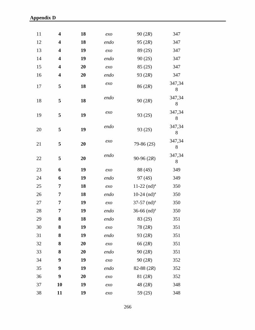
Appendix D
266
11 4 18 exo 90 (2R) 347
12 4 18 endo 95 (2R) 347
13 4 19 exo 89 (2S) 347
14 4 19 endo 90 (2S) 347
15 4 20 exo 85 (2S) 347
16 4 20 endo 93 (2R) 347
17 5 18 exo
86 (2R) 347,34
8
18 5 18 endo
90 (2R) 347,34
8
19 5 19 exo
93 (2S) 347,34
8
20 5 19 endo
93 (2S) 347,34
8
21 5 20 exo
79-86 (2S) 347,34
8
22 5 20 endo
90-96 (2R) 347,34
8
23 6 19 exo 88 (4S) 349
24 6 19 endo 97 (4S) 349
25 7 18 exo 11-22 (nd)a 350
26 7 18 endo 10-24 (nd)a 350
27 7 19 exo 37-57 (nd)a 350
28 7 19 endo 36-66 (nd)a 350
29 8 18 endo 83 (2S) 351
30 8 19 exo 78 (2R) 351
31 8 19 endo 93 (2R) 351
32 8 20 exo 66 (2R) 351
33 8 20 endo 90 (2R) 351
34 9 19 exo 90 (2R) 352
35 9 19 endo 82-88 (2R) 352
36 9 20 exo 81 (2R) 352
37 10 19 exo 48 (2R) 348
38 11 19 exo 59 (2S) 348

Appendix D
267
39 12 19 exo 57 (2R) 348
40 13 19 exo 74 (2R) 348
41 14 19 exo 9 (R) 353
42 14 19 endo 15 (R) 353
43 15 19 exo 38 (S) 353
44 15 19 endo 27 (R) 353
45 16 19 exo 53 (R) 353
46 16 19 endo 39 (R) 353
47 17 18 exo 88 (S) 353
48 17 19 exo 72-92 (R) 353
49 17 19 endo 68-91 (R) 353
a Absolute stereochemistry not assigned.

Appendix D
268
Chart and Table D4: Catalysts and aldehydes set used in the organocatalyzed aldol reaction.
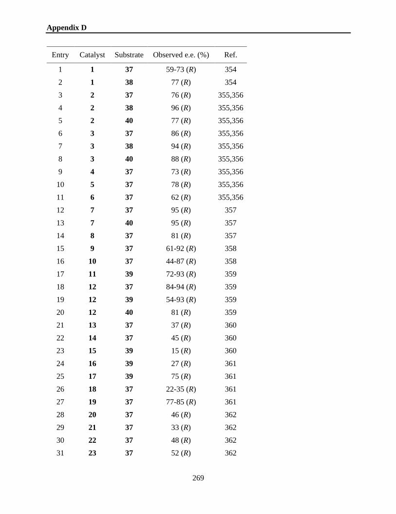
Appendix D
269
Entry Catalyst Substrate Observed e.e. (%) Ref.
1 1 37 59-73 (R) 354
2 1 38 77 (R) 354
3 2 37 76 (R) 355,356
4 2 38 96 (R) 355,356
5 2 40 77 (R) 355,356
6 3 37 86 (R) 355,356
7 3 38 94 (R) 355,356
8 3 40 88 (R) 355,356
9 4 37 73 (R) 355,356
10 5 37 78 (R) 355,356
11 6 37 62 (R) 355,356
12 7 37 95 (R) 357
13 7 40 95 (R) 357
14 8 37 81 (R) 357
15 9 37 61-92 (R) 358
16 10 37 44-87 (R) 358
17 11 39 72-93 (R) 359
18 12 37 84-94 (R) 359
19 12 39 54-93 (R) 359
20 12 40 81 (R) 359
21 13 37 37 (R) 360
22 14 37 45 (R) 360
23 15 39 15 (R) 360
24 16 39 27 (R) 361
25 17 39 75 (R) 361
26 18 37 22-35 (R) 361
27 19 37 77-85 (R) 361
28 20 37 46 (R) 362
29 21 37 33 (R) 362
30 22 37 48 (R) 362
31 23 37 52 (R) 362

Appendix D
270
32 24 37 49 (R) 362
33 25 37 44 (R) 362
34 26 37 64 (R) 362
35 27 37 69-93 (R) 362
36 27 38 98 (R) 362
37 27 40 84 (R) 362
38 28 37 15 (R) 363
39 29 37 72 (R) 363
40 30 37 15 (R) 363
41 31 37 87-99 (R) 363
42 31 38 >99 (R) 363
43 31 39 99 (R) 363
44 32 37 17 (R) 363
45 33 37 67 (R) 363
46 34 37 96 (R) 364
47 35 37 60 (R) 364
48 36 37 95 (R) 364
49 36 40 96 (R) 364

Appendix D
271
Chart and Table D5: Catalysts and substrates set used in the dihydroxylation reaction.
Entry Catalyst Substrate Observed e.e. (%) Ref.
1 1a 1 97 (R) 365,36
6
2 1b 1 97 (S) 365,36
6
3 2a 1 80 (R) 365
4 3a 1 99 (R) 365
5 3b 1 97 (S) 365
6 4a 1 98 (R) 365

Appendix D
272
7 4b 1 96 (S) 365
8 5a 1 96 (R) 366,36
7
9 5b 1 93 (S) 366
10 6a 1 80-92 (R) 366
11 6b 1 79-85 (S) 366
12 7a 1 87 (R) 368
13 8a 1 60-74 (R) 369
368
14 8b 1 54 (S) 369
15 9a 1 78 (R) 368
16 10 1 93 (R) 370
17 11 1 21 (S) 371
18 12a 1 89 (R) 372
19 12b 1 85 (S) 372
20 14 1 76 (R) 367
21 1a 2 94 (R) 365
22 1b 2 93 (S) 365
23 2a 2 69 (R) 365
24 3a 2 96 (R) 365
25 3b 2 92 (S) 365
26 4a 2 94 (R) 365
27 4b 2 94 (S) 365
28 5a 2 93 (R) 366
29 6a 2 72 (R) 366
30 8a 2 33 (R) 369
31 12a 2 82 (R) 372
32 1a 3 >99.5 (R,R) 373
33 1b 3 >99.5 (S,S) 373
34 5a 3 99 (R,R) 367
35 7a 3 98 (R,R) 368
36 8a 3 85-88 (R,R)
99 (R,R)
369
368

Appendix D
273
37 8b 3 78 (S,S) 369
38 9a 3 99 (R,R) 368
39 10 3 99.5 (R,R) 370
40 11 3 40 (S,S) 371
41 14 3 92 (R,R) 367
42 8a 4 65 (R,R) 369
43 8b 4 55 (S,S) 369
44 10 4 97 (R,R) 370
45 11 4 19 (S,S) 371
46 12a 4 92 (R,R) 372
47 1a 5 42 (1R,2S) 365,37
4
48 2a 5 35 (1R,2S) 365,37
4
51 3a 5 20 (1R,2S) 365
50 4a 5 53 (1R,2S) 365
51 11 5 12 (1S 2R) 371
52 12a 5 63 (1R,2S) 372
53 1a 6 64 -
54 1b 6 66 -
55 2a 6 92 -
56 2b 6 87 -
57 3a 6 59 -
58 3b 6 65 -
59 4a 6 67 -
60 4b 6 73 -
61 7a 6 79 (R) -
62 8a 6 44 (R) -
63 9a 6 79 (R) -

Appendix D
274
Chart and Table D6: Catalysts and substrates set used in the diethylzinc addition to aldehyde
reaction.

Appendix D
275
Entry Catalyst Substrate Observed e.e. (%) Ref.
1 1 41a 90 (S) 375
2 1 41c 78 (S) 375
3 1 41d 88 (S) 375
4 2 41a 97 (R) 376,377
5 2 41c 95 (R) 376,377
6 2 41d 88 (R) 376,377
7 3 41a 85 (R) 376,377
8 3 41d 78 (R) 376,377
9 4 41a 67 (R) 376
10 5 41a 98 (S) 378
11 5 41b 90 (S) 378
12 5 41d 61 (S) 378
13 6 41a 24 (R) 379
14 7 41a 75 (S) 379
15 8 41a 24 (S) 379
16 9 41a 68 (R) 380
17 10 41a 81.8 (S) 320
18 11 41a 99 (S)a 381
19 11 41c 99 (S)a 381
20 11 41d 80 (S)a 381
21 12 41a 84 (S) 382
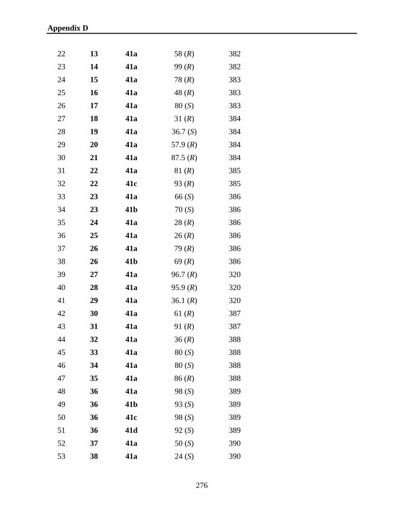
Appendix D
276
22 13 41a 58 (R) 382
23 14 41a 99 (R) 382
24 15 41a 78 (R) 383
25 16 41a 48 (R) 383
26 17 41a 80 (S) 383
27 18 41a 31 (R) 384
28 19 41a 36.7 (S) 384
29 20 41a 57.9 (R) 384
30 21 41a 87.5 (R) 384
31 22 41a 81 (R) 385
32 22 41c 93 (R) 385
33 23 41a 66 (S) 386
34 23 41b 70 (S) 386
35 24 41a 28 (R) 386
36 25 41a 26 (R) 386
37 26 41a 79 (R) 386
38 26 41b 69 (R) 386
39 27 41a 96.7 (R) 320
40 28 41a 95.9 (R) 320
41 29 41a 36.1 (R) 320
42 30 41a 61 (R) 387
43 31 41a 91 (R) 387
44 32 41a 36 (R) 388
45 33 41a 80 (S) 388
46 34 41a 80 (S) 388
47 35 41a 86 (R) 388
48 36 41a 98 (S) 389
49 36 41b 93 (S) 389
50 36 41c 98 (S) 389
51 36 41d 92 (S) 389
52 37 41a 50 (S) 390
53 38 41a 24 (S) 390

Appendix D
277
54 39 41a 97 (S) 390
55 40 41a 29 (R) 390 a This catalyst features an aziridine which does not match with the template used in Constructs.
Chart and Table D7: Ruthenium ligands and substrates set used in the hydrogenation reaction.

Appendix D
278
Entry Catalyst Substrate Observed e.e. (%)a Ref.
1 1 11 29 (S) 391
2 2 11 30 (S) 391
3 3 11 87 (R) 391
4 4 11 86 (S) 391
5 5 11 37 (R) 391
6 6 11 74 (S) 391
7 1 12 67 (S) 391
8 2 12 78 (S) 391
9 3 12 36 (R) 391
10 4 12 94 (S) 391
11 5 12 82 (R) 391
12 6 12 60 (S) 391
13 1 13 30 (S) 391
14 2 13 17 (S) 391
15 3 13 82 (R) 391
16 4 13 96 (S) 391
17 5 13 80 (R) 391
18 6 13 88 (S) 391
19 1 14 49 (S) 391
20 2 14 55 (S) 391
21 3 14 22 (R) 391
22 4 14 95 (S) 391
23 5 14 75 (R) 391
24 6 14 53 (S) 391
25 1 15 18 (S) 391
26 2 15 8 (S) 391
27 3 15 71 (R) 391
28 4 15 65 (S) 391
29 5 15 57 (R) 391
30 6 15 81 (S) 391
31 1 16 54 (S) 391

Appendix D
279
32 2 16 24 (S) 391
33 3 16 24 (R) 391
34 4 16 78 (S) 391
35 5 16 72 (R) 391
36 6 16 67 (S) 391
37 1 17 56 (S) 391
38 2 17 45 (S) 391
39 3 17 79 (R) 391
40 4 17 95 (S) 391
41 5 17 82 (R) 391
42 6 17 80 (S) 391
43 7 17 98 (S)b 392
44 1 18 49 (S) 391
45 4 18 96 (S) 391,393
46 5 18 95 (R) 391
47 7 18 99 (S)b 392
48 8 18 21 (R)b 394
49 1 19 83 (S) 393
50 3 19 95 +(R) 393
51 4 19 95 (S) 393
52 5 19 91 (R) 393
53 7 19 99 (S)b 392
54 8 19 15 (R)b 394
55 4 20 55 (S) 391
56 5 20 0 391
57 9 20 96 (R) 310
58 10 20 98.2 (R) 310
59 9 21 96.2 (R) 310
60 10 21 97.5 (R) 310
61 9 22 85.1 (R) 310
62 10 22 96.8 (R) 310
63 9 23 96.8 (R) 310
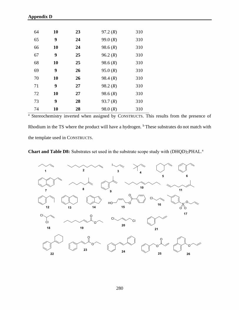
Appendix D
280
64 10 23 97.2 (R) 310
65 9 24 99.0 (R) 310
66 10 24 98.6 (R) 310
67 9 25 96.2 (R) 310
68 10 25 98.6 (R) 310
69 9 26 95.0 (R) 310
70 10 26 98.4 (R) 310
71 9 27 98.2 (R) 310
72 10 27 98.6 (R) 310
73 9 28 93.7 (R) 310
74 10 28 98.0 (R) 310 a Stereochemistry inverted when assigned by CONSTRUCTS. This results from the presence of
Rhodium in the TS where the product will have a hydrogen. b These substrates do not match with
the template used in CONSTRUCTS.
Chart and Table D8: Substrates set used in the substrate scope study with (DHQD)2PHAL.a

Appendix D
281
Entry Substrate Observed e.e. (%) Ref.
1 1 79 (R) 365
2 2 84 (R) 365
3 3 63 (S) 365
4 4 64 (R) 365
5 5 88 (R) 365
6 6 97 (R) 365
7 7 99 (R) 365
8 8 78 (R) 365
9 9 94 (R) 365
10 10 97 (R,R) 365
11 11b 98 (R) 365
12 12 35 (1R,2S) 365
13 13 15 (1R,2S) 365
14 14 42 (1R,2S) 365
15 15 64 (1S,2R) 365
16 16 63 (S) 372
17 17 40 (S) 372
18 18 63 (S) 372
19 19 99 (2S,3R) 372
20 20 94 (S,S) 372
21 21 44 (R) 372
22 22 99 (R,R) 373
23 23 97 (2S, 2R) 373
24 24 >99.5 (R,R) 373
25 25 77 (S) 373
26 26 91 (S) 373 a (DHQD)2PHAL is catalyst 1a in Table D5. b the two double bonds cannot be distinguished by
CONSTRUCTS. This substrate was discarded.

Chapter 7
282
Chapter 7 – References
(1) Council, N. R.: Mathematical Challenges from Theoretical/Computational
Chemistry; The National Academies Press: Washington, DC, 1995.
(2) Lipkowitz, K. B.; Boyd, D. B.: Reviews in Computational Chemistry - Volume 1,
1990.
(3) W. J. Hehre; W. A. Lathan; R. Ditchfield; M. D. Newton, a.; Pople, J. A. Gaussian
70 (Quantum Chemistry Program Exchange, Program No. 237, 1970). 1970.
(4) DelMonte, A. J.; Haller, J.; Houk, K. N.; Sharpless, K. B.; Singleton, D. A.;
Strassner, T.; Thomas, A. A. Experimental and Theoretical Kinetic Isotope Effects for Asymmetric
Dihydroxylation. Evidence Supporting a Rate-Limiting “(3 + 2)” Cycloaddition. Journal of the
American Chemical Society 1997, 119, 9907-9908.
(5) McCammon, J. A.; Gelin, B. R.; Karplus, M. Dynamics of folded proteins. Nature
1977, 267, 585-590.
(6) The Nobel Prize in Chemistry 1998. (accessed January 21 2020).
(7) The Nobel Prize in Chemistry 2013. (accessed January 21 2020).
(8) Cornell, W. D.; Cieplak, P.; Bayly, C. I.; Gould, I. R.; Merz, K. M.; Ferguson, D.
M.; Spellmeyer, D. C.; Fox, T.; Caldwell, J. W.; Kollman, P. A. A Second Generation Force Field
for the Simulation of Proteins, Nucleic Acids, and Organic Molecules J. Am. Chem. Soc. 1995,
117, 5179−5197. Journal of the American Chemical Society 1996, 118, 2309-2309.
(9) Wang, J.; Wolf, R. M.; Caldwell, J. W.; Kollman, P. A.; Case, D. A. Development
and testing of a general amber force field. Journal of Computational Chemistry 2004, 25, 1157-
1174.
(10) Harder, E.; Damm, W.; Maple, J.; Wu, C.; Reboul, M.; Xiang, J. Y.; Wang, L.;
Lupyan, D.; Dahlgren, M. K.; Knight, J. L.; Kaus, J. W.; Cerutti, D. S.; Krilov, G.; Jorgensen, W.
L.; Abel, R.; Friesner, R. A. OPLS3: A Force Field Providing Broad Coverage of Drug-like Small
Molecules and Proteins. Journal of Chemical Theory and Computation 2016, 12, 281-296.
(11) Champion, C.; Barigye, S. J.; Wei, W.; Liu, Z.; Labute, P.; Moitessier, N. Atom
Type Independent Modeling of the Conformational Energy of Benzylic, Allylic, and Other Bonds
Adjacent to Conjugated Systems. Journal of Chemical Information and Modeling 2019, 59, 4750-
4763.
(12) Vanommeslaeghe, K.; Guvench, O.; MacKerell, A. D., Jr. Molecular mechanics.
Curr Pharm Des 2014, 20, 3281-3292.
(13) Clobazam in Treatment of Refractory Epilepsy: The Canadian Experience. A
Retrospecti. Epilepsia 1991, 32, 407-416.
(14) Mobley, D. L.; Bannan, C. C.; Rizzi, A.; Bayly, C. I.; Chodera, J. D.; Lim, V. T.;
Lim, N. M.; Beauchamp, K. A.; Shirts, M. R.; Gilson, M. K.; Eastman, P. K. Open Force Field
Consortium: Escaping atom types using direct chemical perception with SMIRNOFF v0.1. bioRxiv
2018, 286542.
(15) Lengauer, T.; Rarey, M. Computational methods for biomolecular docking.
Current Opinion in Structural Biology 1996, 6, 402-406.
(16) Khanna, V.; Ranganathan, S.; Petrovsky, N.: Rational Structure-Based Drug
Design. In Encyclopedia of Bioinformatics and Computational Biology; Ranganathan, S.,
Gribskov, M., Nakai, K., Schönbach, C., Eds.; Academic Press: Oxford, 2019; pp 585-600.

Chapter 7
283
(17) Voelz, V. A.; Bowman, G. R.; Beauchamp, K.; Pande, V. S. Molecular simulation
of ab initio protein folding for a millisecond folder NTL9(1-39). Journal of the American Chemical
Society 2010, 132, 1526-1528.
(18) Burai Patrascu, M.; Pottel, J.; Pinus, S.; Bezanson, M.; Norrby, P.-O.; Moitessier,
N. From Desktop to Benchtop – A Paradigm Shift in Asymmetric Synthesis. ChemRxiv 2019.
(19) Ren, P.; Wu, C.; Ponder, J. W. Polarizable Atomic Multipole-Based Molecular
Mechanics for Organic Molecules. Journal of Chemical Theory and Computation 2011, 7, 3143-
3161.
(20) Roothaan, C. C. J. New Developments in Molecular Orbital Theory. Reviews of
Modern Physics 1951, 23, 69-89.
(21) Kohn, W.; Sham, L. J. Self-Consistent Equations Including Exchange and
Correlation Effects. Physical Review 1965, 140, A1133-A1138.
(22) Pople, J. A.; Beveridge, D. L.; Dobosh, P. A. Approximate Self‐Consistent
Molecular‐Orbital Theory. V. Intermediate Neglect of Differential Overlap. The Journal of
Chemical Physics 1967, 47, 2026-2033.
(23) Szabo, A.; Ostlund, N. S.: Modern quantum chemistry : introduction to advanced
electronic structure theory; 1st ed., Rev. ed.; McGraw-Hill: New York, 1989. pp. xiv, 466 pages :
illustrations ; 24 cm.
(24) Christensen, A. S.; Kubař, T.; Cui, Q.; Elstner, M. Semiempirical Quantum
Mechanical Methods for Noncovalent Interactions for Chemical and Biochemical Applications.
Chemical Reviews 2016, 116, 5301-5337.
(25) Barone, V.; Arnaud, R. Study of prototypical Diels-Alder reactions by a hybrid
density functional/Hartree-Fock approach. Chemical Physics Letters 1996, 251, 393-399.
(26) Barone, V.; Adamo, C. A theoretical investigation of potential energy surfaces
governing the photochemical tautomerization of 2-pyridone. Chemical Physics Letters 1994, 226,
399-404.
(27) Burai Patrascu, M.; Plescia, J.; Kalgutkar, A.; Mascitti, V.; Moitessier, N.
Computational methods for prediction of drug properties - application to Cytochrome P450
metabolism prediction. Arkivoc 2019, 2019, 280-298.
(28) Dewar, M. J. S.; Zoebisch, E. G.; Healy, E. F.; Stewart, J. J. P. Development and
use of quantum mechanical molecular models. 76. AM1: a new general purpose quantum
mechanical molecular model. Journal of the American Chemical Society 1985, 107, 3902-3909.
(29) Stewart, J. J. P. Optimization of parameters for semiempirical methods II.
Applications. Journal of Computational Chemistry 1989, 10, 221-264.
(30) Stewart, J. J. P. Optimization of parameters for semiempirical methods V:
Modification of NDDO approximations and application to 70 elements. Journal of Molecular
Modeling 2007, 13, 1173-1213.
(31) Rocha, G. B.; Freire, R. O.; Simas, A. M.; Stewart, J. J. P. RM1: A
reparameterization of AM1 for H, C, N, O, P, S, F, Cl, Br, and I. Journal of Computational
Chemistry 2006, 27, 1101-1111.
(32) Bikadi, Z.; Hazai, E. Application of the PM6 semi-empirical method to modeling
proteins enhances docking accuracy of AutoDock. Journal of Cheminformatics 2009, 1, 15.
(33) Matsuzawa, N.; Dixon, D. A. Semiempirical calculations of hyperpolarizabilities
for donor-acceptor molecules: comparison to experiment. The Journal of Physical Chemistry 1992,
96, 6232-6241.

Chapter 7
284
(34) Stewart, J. J. P. Application of the PM6 method to modeling proteins. Journal of
Molecular Modeling 2009, 15, 765-805.
(35) Muddana, H. S.; Gilson, M. K. Calculation of Host–Guest Binding Affinities Using
a Quantum-Mechanical Energy Model. Journal of Chemical Theory and Computation 2012, 8,
2023-2033.
(36) Korth, M. Third-Generation Hydrogen-Bonding Corrections for Semiempirical
QM Methods and Force Fields. Journal of Chemical Theory and Computation 2010, 6, 3808-3816.
(37) Becke, A. D. Density‐functional thermochemistry. III. The role of exact exchange.
The Journal of Chemical Physics 1993, 98, 5648-5652.
(38) Lee, C.; Yang, W.; Parr, R. G. Development of the Colle-Salvetti correlation-
energy formula into a functional of the electron density. Physical Review B 1988, 37, 785-789.
(39) Becke, A. D. Perspective: Fifty years of density-functional theory in chemical
physics. The Journal of Chemical Physics 2014, 140, 18A301.
(40) Neese, F. Software update: the ORCA program system, version 4.0. WIREs
Computational Molecular Science 2018, 8, e1327.
(41) Schmidt, M. W.; Baldridge, K. K.; Boatz, J. A.; Elbert, S. T.; Gordon, M. S.; Jensen,
J. H.; Koseki, S.; Matsunaga, N.; Nguyen, K. A.; Su, S.; Windus, T. L.; Dupuis, M.; Montgomery,
J. A. General atomic and molecular electronic structure system. J. Comp. Chem. 1993, 14, 1347-
1363.
(42) Gordon, M. S.; Schmidt, M. W.: Advances in electronic structure theory: GAMESS
a decade later. In Theory and Applications of Computational Chemistry: the first forty years;
Dykstra, C. E., Frenking, G., Kim, K. S., Scuseria, G. E., Eds.; Elsevier, 2005; pp 1167-1189.
(43) Vondrášek, J.; Bendová, L.; Klusák, V.; Hobza, P. Unexpectedly Strong Energy
Stabilization Inside the Hydrophobic Core of Small Protein Rubredoxin Mediated by Aromatic
Residues: Correlated Ab Initio Quantum Chemical Calculations. Journal of the American
Chemical Society 2005, 127, 2615-2619.
(44) Grimme, S. Density functional theory with London dispersion corrections. WIREs
Computational Molecular Science 2011, 1, 211-228.
(45) Grimme, S.; Brandenburg, J. G.; Bannwarth, C.; Hansen, A. Consistent structures
and interactions by density functional theory with small atomic orbital basis sets. The Journal of
Chemical Physics 2015, 143, 054107.
(46) Brandenburg, J. G.; Bannwarth, C.; Hansen, A.; Grimme, S. B97-3c: A revised
low-cost variant of the B97-D density functional method. The Journal of Chemical Physics 2018,
148, 064104.
(47) Lundberg, M.; Siegbahn, P. E. M. Quantifying the effects of the self-interaction
error in DFT: When do the delocalized states appear? The Journal of Chemical Physics 2005, 122,
224103.
(48) Harvey, J. N. On the accuracy of density functional theory in transition metal
chemistry. Annual Reports Section "C" (Physical Chemistry) 2006, 102, 203-226.
(49) Marques, A. N. L.; Mendes Filho, J.; Freire, P. T. C.; Santos, H. S.; Albuquerque,
M. R. J. R.; Bandeira, P. N.; Leite, R. V.; Braz-Filho, R.; Gusmão, G. O. M.; Nogueira, C. E. S.;
Teixeira, A. M. R. Vibrational spectroscopy and DFT calculations of flavonoid derriobtusone A.
Journal of Molecular Structure 2017, 1130, 231-237.
(50) Cresswell, A. J.; Eey, S. T. C.; Denmark, S. E. Catalytic, stereospecific syn-
dichlorination of alkenes. Nature Chemistry 2015, 7, 146-152.
Chapter 7
285
(51) Fu, L.; Mu, X.; Li, B. Reaction mechanism of organoselenium-catalyzed syn-
dichlorination of alkenes: a DFT study. Journal of Molecular Modeling 2018, 24, 91.
(52) Fleming, E. M.; Quigley, C.; Rozas, I.; Connon, S. J. Computational Study-Led
Organocatalyst Design: A Novel, Highly Active Urea-Based Catalyst for Addition Reactions to
Epoxides. The Journal of Organic Chemistry 2008, 73, 948-956.
(53) Ainsley, J.; Lodola, A.; Mulholland, A. J.; Christov, C. Z.; Karabencheva-
Christova, T. G.: Chapter One - Combined Quantum Mechanics and Molecular Mechanics Studies
of Enzymatic Reaction Mechanisms. In Advances in Protein Chemistry and Structural Biology;
Karabencheva-Christova, T. G., Christov, C. Z., Eds.; Academic Press, 2018; Vol. 113; pp 1-32.
(54) Karabencheva-Christova, T. G.; Torras, J.; Mulholland, A. J.; Lodola, A.; Christov,
C. Z. Mechanistic Insights into the Reaction of Chlorination of Tryptophan Catalyzed by
Tryptophan 7-Halogenase. Scientific Reports 2017, 7, 17395.
(55) Chaskar, P.; Zoete, V.; Röhrig, U. F. On-the-Fly QM/MM Docking with Attracting
Cavities. Journal of Chemical Information and Modeling 2017, 57, 73-84.
(56) Senn, H. M.; Thiel, W.: QM/MM Methods for Biological Systems. In Atomistic
Approaches in Modern Biology: From Quantum Chemistry to Molecular Simulations; Reiher, M.,
Ed.; Springer Berlin Heidelberg: Berlin, Heidelberg, 2007; pp 173-290.
(57) Ibragimova, G. T.; Wade, R. C. Importance of Explicit Salt Ions for Protein
Stability in Molecular Dynamics Simulation. Biophysical Journal 1998, 74, 2906-2911.
(58) Cova, T. F. G. G.; Pais, A. A. C. C. Deep Learning for Deep Chemistry: Optimizing
the Prediction of Chemical Patterns. Frontiers in Chemistry 2019, 7, 809.
(59) Hirohara, M.; Saito, Y.; Koda, Y.; Sato, K.; Sakakibara, Y. Convolutional neural
network based on SMILES representation of compounds for detecting chemical motif. BMC
Bioinformatics 2018, 19, 526.
(60) Hiller, S. A.; Golender, V. E.; Rosenblit, A. B.; Rastrigin, L. A.; Glaz, A. B.
Cybernetic methods of drug design. I. Statement of the problem—The perceptron approach.
Computers and Biomedical Research 1973, 6, 411-421.
(61) Jaén-Oltra, J.; Salabert-Salvador, M. T.; García-March, F. J.; Pérez-Giménez, F.;
Tomás-Vert, F. Artificial Neural Network Applied to Prediction of Fluorquinolone Antibacterial
Activity by Topological Methods. Journal of Medicinal Chemistry 2000, 43, 1143-1148.
(62) Zhou, Y.; Cahya, S.; Combs, S. A.; Nicolaou, C. A.; Wang, J.; Desai, P. V.; Shen,
J. Exploring Tunable Hyperparameters for Deep Neural Networks with Industrial ADME Data
Sets. Journal of Chemical Information and Modeling 2019, 59, 1005-1016.
(63) Zaretzki, J.; Matlock, M.; Swamidass, S. J. XenoSite: Accurately Predicting CYP-
Mediated Sites of Metabolism with Neural Networks. Journal of Chemical Information and
Modeling 2013, 53, 3373-3383.
(64) Svetnik, V.; Liaw, A.; Tong, C.; Culberson, J. C.; Sheridan, R. P.; Feuston, B. P.
Random Forest: A Classification and Regression Tool for Compound Classification and QSAR
Modeling. Journal of Chemical Information and Computer Sciences 2003, 43, 1947-1958.
(65) Wang, C.; Zhang, Y. Improving scoring-docking-screening powers of protein–
ligand scoring functions using random forest. Journal of Computational Chemistry 2017, 38, 169-
177.
(66) Finkelmann, A. R.; Göller, A. H.; Schneider, G. Site of Metabolism Prediction
Based on ab initio Derived Atom Representations. ChemMedChem 2017, 12, 606-612.
(67) Dalvie, D.; Kalgutkar, A. S.; Chen, W. Practical approaches to resolving reactive
metabolite liabilities in early discovery. Drug Metabolism Reviews 2015, 47, 56-70.

Chapter 7
286
(68) Kaitin, K. I. Deconstructing the Drug Development Process: The New Face of
Innovation. Clinical Pharmacology & Therapeutics 2010, 87, 356-361.
(69) Taft, C. A.; da Silva, V. B.; da Silva, C. H. T. d. P. Current topics in computer‐
aided drug design. Journal of Pharmaceutical Sciences 2008, 97, 1089-1098.
(70) Aparoy, P.; Reddy, K. K.; Reddanna, P. Structure and ligand based drug design
strategies in the development of novel 5- LOX inhibitors. Curr Med Chem 2012, 19, 3763-3778.
(71) Corbeil, C. R.; Englebienne, P.; Moitessier, N. Docking Ligands into Flexible and
Solvated Macromolecules. 1. Development and Validation of FITTED 1.0. Journal of Chemical
Information and Modeling 2007, 47, 435-449.
(72) Pagadala, N. S.; Syed, K.; Tuszynski, J. Software for molecular docking: a review.
Biophys Rev 2017, 9, 91-102.
(73) Koshland Jr, D. E. The Key–Lock Theory and the Induced Fit Theory. Angewandte
Chemie International Edition in English 1995, 33, 2375-2378.
(74) Forli, S.; Huey, R.; Pique, M. E.; Sanner, M. F.; Goodsell, D. S.; Olson, A. J.
Computational protein-ligand docking and virtual drug screening with the AutoDock suite. Nat
Protoc 2016, 11, 905-919.
(75) Friesner, R. A.; Banks, J. L.; Murphy, R. B.; Halgren, T. A.; Klicic, J. J.; Mainz, D.
T.; Repasky, M. P.; Knoll, E. H.; Shelley, M.; Perry, J. K.; Shaw, D. E.; Francis, P.; Shenkin, P.
S. Glide: A New Approach for Rapid, Accurate Docking and Scoring. 1. Method and Assessment
of Docking Accuracy. Journal of Medicinal Chemistry 2004, 47, 1739-1749.
(76) Jones, G.; Willett, P.; Glen, R. C.; Leach, A. R.; Taylor, R. Development and
validation of a genetic algorithm for flexible docking11Edited by F. E. Cohen. Journal of
Molecular Biology 1997, 267, 727-748.
(77) von Itzstein, M.; Wu, W.-Y.; Kok, G. B.; Pegg, M. S.; Dyason, J. C.; Jin, B.; Van
Phan, T.; Smythe, M. L.; White, H. F.; Oliver, S. W.; Colman, P. M.; Varghese, J. N.; Ryan, D.
M.; Woods, J. M.; Bethell, R. C.; Hotham, V. J.; Cameron, J. M.; Penn, C. R. Rational design of
potent sialidase-based inhibitors of influenza virus replication. Nature 1993, 363, 418-423.
(78) Jenwitheesuk, E.; Samudrala, R. Improved prediction of HIV-1 protease-inhibitor
binding energies by molecular dynamics simulations. BMC Struct Biol 2003, 3, 2-2.
(79) Irwin, J. J.; Shoichet, B. K. ZINC--a free database of commercially available
compounds for virtual screening. Journal of chemical information and modeling 2005, 45, 177-
182.
(80) Hoffmann, T.; Gastreich, M. The next level in chemical space navigation: going far
beyond enumerable compound libraries. Drug Discovery Today 2019, 24, 1148-1156.
(81) Therrien, E.; Englebienne, P.; Arrowsmith, A. G.; Mendoza-Sanchez, R.; Corbeil,
C. R.; Weill, N.; Campagna-Slater, V.; Moitessier, N. Integrating Medicinal Chemistry,
Organic/Combinatorial Chemistry, and Computational Chemistry for the Discovery of Selective
Estrogen Receptor Modulators with Forecaster, a Novel Platform for Drug Discovery. Journal of
Chemical Information and Modeling 2012, 52, 210-224.
(82) Kuck, D.; Singh, N.; Lyko, F.; Medina-Franco, J. L. Novel and selective DNA
methyltransferase inhibitors: Docking-based virtual screening and experimental evaluation.
Bioorganic & Medicinal Chemistry 2010, 18, 822-829.
(83) Wang, D.; Wang, F.; Tan, Y.; Dong, L.; Chen, L.; Zhu, W.; Wang, H. Discovery
of potent small molecule inhibitors of DYRK1A by structure-based virtual screening and bioassay.
Bioorganic & Medicinal Chemistry Letters 2012, 22, 168-171.

Chapter 7
287
(84) Hospital, A.; Goñi, J. R.; Orozco, M.; Gelpí, J. L. Molecular dynamics simulations:
advances and applications. Adv Appl Bioinform Chem 2015, 8, 37-47.
(85) Kmiecik, S.; Gront, D.; Kolinski, M.; Wieteska, L.; Dawid, A. E.; Kolinski, A.
Coarse-Grained Protein Models and Their Applications. Chemical Reviews 2016, 116, 7898-7936.
(86) Nelson, M. T.; Humphrey, W.; Gursoy, A.; Dalke, A.; Kalé, L. V.; Skeel, R. D.;
Schulten, K. NAMD: a Parallel, Object-Oriented Molecular Dynamics Program. The International
Journal of Supercomputer Applications and High Performance Computing 1996, 10, 251-268.
(87) Schames, J. R.; Henchman, R. H.; Siegel, J. S.; Sotriffer, C. A.; Ni, H.;
McCammon, J. A. Discovery of a Novel Binding Trench in HIV Integrase. Journal of Medicinal
Chemistry 2004, 47, 1879-1881.
(88) Durrant, J. D.; McCammon, J. A. Molecular dynamics simulations and drug
discovery. BMC Biology 2011, 9, 71.
(89) Zeevaart, J. G.; Wang, L.; Thakur, V. V.; Leung, C. S.; Tirado-Rives, J.; Bailey, C.
M.; Domaoal, R. A.; Anderson, K. S.; Jorgensen, W. L. Optimization of Azoles as Anti-Human
Immunodeficiency Virus Agents Guided by Free-Energy Calculations. Journal of the American
Chemical Society 2008, 130, 9492-9499.
(90) Acharya, C.; Coop, A.; Polli, J. E.; Mackerell, A. D., Jr. Recent advances in ligand-
based drug design: relevance and utility of the conformationally sampled pharmacophore
approach. Curr Comput Aided Drug Des 2011, 7, 10-22.
(91) Cramer, R. D.; Patterson, D. E.; Bunce, J. D. Comparative molecular field analysis
(CoMFA). 1. Effect of shape on binding of steroids to carrier proteins. Journal of the American
Chemical Society 1988, 110, 5959-5967.
(92) Klebe, G.; Abraham, U.; Mietzner, T. Molecular Similarity Indices in a
Comparative Analysis (CoMSIA) of Drug Molecules to Correlate and Predict Their Biological
Activity. Journal of Medicinal Chemistry 1994, 37, 4130-4146.
(93) Kuo, C.-L.; Assefa, H.; Kamath, S.; Brzozowski, Z.; Slawinski, J.; Saczewski, F.;
Buolamwini, J. K.; Neamati, N. Application of CoMFA and CoMSIA 3D-QSAR and Docking
Studies in Optimization of Mercaptobenzenesulfonamides as HIV-1 Integrase Inhibitors. Journal
of Medicinal Chemistry 2004, 47, 385-399.
(94) Shaldam, M.; Tawfik, H.; El-Bastawissy, E.; El-Moselhy, T. The Application of
CoMFA Approach for the Design of 1,4-Dihydropyridines as Calcium Channel Blockers.
CHEMISTRY and BIOLOGY INTERFACE 2016, 6, 350-356.
(95) Ehrlich, P. Über den jetzigen Stand der Chemotherapie. Berichte der deutschen
chemischen Gesellschaft 1909, 42, 17-47.
(96) Schueler, F. W. Chemobiodynamics and Drug Design. Journal of Pharmaceutical
Sciences 1961, 50.
(97) Wermuth, C.-G.; Robin Ganellin, C.; Lindberg, P.; Mitscher, L. A.: Chapter 36 -
Glossary of Terms Used in Medicinal Chemistry (IUPAC Recommendations 1997). In Annual
Reports in Medicinal Chemistry; Bristol, J. A., Ed.; Academic Press, 1998; Vol. 33; pp 385-395.
(98) Yang, S.-Y. Pharmacophore modeling and applications in drug discovery:
challenges and recent advances. Drug Discovery Today 2010, 15, 444-450.
(99) Toba, S.; Srinivasan, J.; Maynard, A. J.; Sutter, J. Using Pharmacophore Models
To Gain Insight into Structural Binding and Virtual Screening: An Application Study with CDK2
and Human DHFR. Journal of Chemical Information and Modeling 2006, 46, 728-735.

Chapter 7
288
(100) Hecker, E. A.; Duraiswami, C.; Andrea, T. A.; Diller, D. J. Use of Catalyst
Pharmacophore Models for Screening of Large Combinatorial Libraries. Journal of Chemical
Information and Computer Sciences 2002, 42, 1204-1211.
(101) Vadivelan, S.; Sinha, B. N.; Irudayam, S. J.; Jagarlapudi, S. A. R. P. Virtual
Screening Studies to Design Potent CDK2-Cyclin A Inhibitors. Journal of Chemical Information
and Modeling 2007, 47, 1526-1535.
(102) Ren, J.-X.; Li, L.-L.; Zou, J.; Yang, L.; Yang, J.-L.; Yang, S.-Y. Pharmacophore
modeling and virtual screening for the discovery of new transforming growth factor-β type I
receptor (ALK5) inhibitors. European Journal of Medicinal Chemistry 2009, 44, 4259-4265.
(103) Wei, D.; Jiang, X.; Zhou, L.; Chen, J.; Chen, Z.; He, C.; Yang, K.; Liu, Y.; Pei, J.;
Lai, L. Discovery of Multitarget Inhibitors by Combining Molecular Docking with Common
Pharmacophore Matching. Journal of Medicinal Chemistry 2008, 51, 7882-7888.
(104) Steindl, T. M.; Schuster, D.; Laggner, C.; Langer, T. Parallel Screening: A Novel
Concept in Pharmacophore Modeling and Virtual Screening. Journal of Chemical Information and
Modeling 2006, 46, 2146-2157.
(105) Law, J.; Zsoldos, Z.; Simon, A.; Reid, D.; Liu, Y.; Khew, S. Y.; Johnson, A. P.;
Major, S.; Wade, R. A.; Ando, H. Y. Route Designer: A Retrosynthetic Analysis Tool Utilizing
Automated Retrosynthetic Rule Generation. Journal of Chemical Information and Modeling 2009,
49, 593-602.
(106) Blurock, E. S. Computer-aided synthesis design at RISC-Linz: automatic extraction
and use of reaction classes. Journal of Chemical Information and Computer Sciences 1990, 30,
505-510.
(107) Kayala, M. A.; Baldi, P. ReactionPredictor: Prediction of Complex Chemical
Reactions at the Mechanistic Level Using Machine Learning. Journal of Chemical Information
and Modeling 2012, 52, 2526-2540.
(108) Feng, F.; Lai, L.; Pei, J. Computational Chemical Synthesis Analysis and Pathway
Design. Frontiers in Chemistry 2018, 6, 199.
(109) Wu, J.; Magrakvelidze, M.; Schmidt, L. P. H.; Kunitski, M.; Pfeifer, T.; Schöffler,
M.; Pitzer, M.; Richter, M.; Voss, S.; Sann, H.; Kim, H.; Lower, J.; Jahnke, T.; Czasch, A.;
Thumm, U.; Dörner, R. Understanding the role of phase in chemical bond breaking with
coincidence angular streaking. Nature Communications 2013, 4, 2177.
(110) Cheng, G.-J.; Zhang, X.; Chung, L. W.; Xu, L.; Wu, Y.-D. Computational Organic
Chemistry: Bridging Theory and Experiment in Establishing the Mechanisms of Chemical
Reactions. Journal of the American Chemical Society 2015, 137, 1706-1725.
(111) Heravi, M. M.; Zadsirjan, V.; Esfandyari, M.; Lashaki, T. B. Applications of
sharpless asymmetric dihydroxylation in the total synthesis of natural products. Tetrahedron:
Asymmetry 2017, 28, 987-1043.
(112) Hentges, S. G.; Sharpless, K. B. Asymmetric induction in the reaction of osmium
tetroxide with olefins. Journal of the American Chemical Society 1980, 102, 4263-4265.
(113) Corey, E. J.; Jardine, P. D.; Virgil, S.; Yuen, P. W.; Connell, R. D. Enantioselective
vicinal hydroxylation of terminal and E-1,2-disubstituted olefins by a chiral complex of osmium
tetroxide. An effective controller system and a rational mechanistic model. Journal of the
American Chemical Society 1989, 111, 9243-9244.
(114) Tomberg, A.; Pottel, J.; Liu, Z.; Labute, P.; Moitessier, N. Understanding P450-
mediated Bio-transformations into Epoxide and Phenolic Metabolites. Angewandte Chemie
International Edition 2015, 54, 13743-13747.

Chapter 7
289
(115) Chattaraj, P. K.; Roy, D. R.: Chapter 9 - Conceptual Density Functional Theory of
Chemical Reactivity. In Advances in Mathematical Chemistry and Applications; Basak, S. C.,
Restrepo, G., Villaveces, J. L., Eds.; Bentham Science Publishers, 2015; pp 196-221.
(116) Kohn, W.; Becke, A. D.; Parr, R. G. Density Functional Theory of Electronic
Structure. The Journal of Physical Chemistry 1996, 100, 12974-12980.
(117) Pearson, R. G. Hard and soft acids and bases—the evolution of a chemical concept.
Coordination Chemistry Reviews 1990, 100, 403-425.
(118) Parr, R. G.; Szentpály, L. v.; Liu, S. Electrophilicity Index. Journal of the American
Chemical Society 1999, 121, 1922-1924.
(119) Parr, R. G.; Yang, W. Density functional approach to the frontier-electron theory
of chemical reactivity. Journal of the American Chemical Society 1984, 106, 4049-4050.
(120) Fukui, K. Role of Frontier Orbitals in Chemical Reactions. Science 1982, 218, 747.
(121) Martinez, C.; Rivera, J. L.; Herrera, R.; Rico, J. L.; Flores, N.; Rutiaga, J. G.; López,
P. Evaluation of the chemical reactivity in lignin precursors using the Fukui function. Journal of
Molecular Modeling 2007, 14, 77.
(122) Mendez, F.; Gazquez, J. L. Chemical Reactivity of Enolate Ions: The Local Hard
and Soft Acids and Bases Principle Viewpoint. Journal of the American Chemical Society 1994,
116, 9298-9301.
(123) Corbeil, C. R.; Thielges, S.; Schwartzentruber, J. A.; Moitessier, N. Toward a
Computational Tool Predicting the Stereochemical Outcome of Asymmetric Reactions:
Development and Application of a Rapid and Accurate Program Based on Organic Principles.
Angewandte Chemie International Edition 2008, 47, 2635-2638.
(124) Rosales, A. R.; Quinn, T. R.; Wahlers, J.; Tomberg, A.; Zhang, X.; Helquist, P.;
Wiest, O.; Norrby, P.-O. Application of Q2MM to predictions in stereoselective synthesis.
Chemical Communications 2018, 54, 8294-8311.
(125) Houk, K. N.; Cheong, P. H.-Y. Computational prediction of small-molecule
catalysts. Nature 2008, 455, 309-313.
(126) Du, X.; Gao, X.; Hu, W.; Yu, J.; Luo, Z.; Cen, K. Catalyst Design Based on DFT
Calculations: Metal Oxide Catalysts for Gas Phase NO Reduction. The Journal of Physical
Chemistry C 2014, 118, 13617-13622.
(127) Wheeler, S. E.; Seguin, T. J.; Guan, Y.; Doney, A. C. Noncovalent Interactions in
Organocatalysis and the Prospect of Computational Catalyst Design. Accounts of Chemical
Research 2016, 49, 1061-1069.
(128) Reid, J. P.; Simón, L.; Goodman, J. M. A Practical Guide for Predicting the
Stereochemistry of Bifunctional Phosphoric Acid Catalyzed Reactions of Imines. Accounts of
Chemical Research 2016, 49, 1029-1041.
(129) Andrea N., B.; Steven, W.: Popular Integration Grids Can Result in Large Errors
in DFT-Computed Free Energies, 2019.
(130) Rosales, A. R.; Wahlers, J.; Limé, E.; Meadows, R. E.; Leslie, K. W.; Savin, R.;
Bell, F.; Hansen, E.; Helquist, P.; Munday, R. H.; Wiest, O.; Norrby, P.-O. Rapid virtual screening
of enantioselective catalysts using CatVS. Nature Catalysis 2019, 2, 41-45.
(131) Hansen, E.; Rosales, A. R.; Tutkowski, B.; Norrby, P.-O.; Wiest, O. Prediction of
Stereochemistry using Q2MM. Accounts of Chemical Research 2016, 49, 996-1005.
(132) Eksterowicz, J. E.; Houk, K. N. Transition-state modeling with empirical force
fields. Chemical Reviews 1993, 93, 2439-2461.
(133) Schrödinger Suite v.2017-2.

Chapter 7
290
(134) Nagata, S.; Tsuchiya, M.; Asano, S.; Kaziro, Y.; Yamazaki, T.; Yamamoto, O.;
Hirata, Y.; Kubota, N.; Oheda, M.; Nomura, H.; Ono, M. Molecular cloning and expression of
cDNA for human granulocyte colony-stimulating factor. Nature 1986, 319, 415-418.
(135) Stein, C. A.; Castanotto, D. FDA-Approved Oligonucleotide Therapies in 2017.
Mol. Ther. 2017, 25, 1069-1075.
(136) Dolgin, E. Spinal muscular atrophy approval boosts antisense drugs. Nat. Biotech.
2017, 35, 99-100.
(137) Broder, S. The development of antiretroviral therapy and its impact on the HIV-
1/AIDS pandemic. Antiviral Res. 2010, 85, 1.
(138) Soudeyns, H.; Yao, X. I.; Gao, Q.; Belleau, B.; Kraus, J. L.; Nguyen-Ba, N.; Spira,
B.; Wainberg, M. A. Anti-human immunodeficiency virus type 1 activity and in vitro toxicity of
2'-deoxy-3'-thiacytidine (BCH-189), a novel heterocyclic nucleoside analog. Antimicrob. Agents
and Chemother. 1991, 35, 1386-1390.
(139) Liotta, D. C.; Painter, G. R. Discovery and Development of the Anti-Human
Immunodeficiency Virus Drug, Emtricitabine (Emtriva, FTC). Acc. Chem. Res. 2016, 49, 2091-
2098.
(140) Dienstag, J.; Easley, C.; Kirkpatrick, P. Telbivudine. Nat. Rev. Drug Discov. 2007,
6, 267-268.
(141) Warren, T. K.; Wells, J.; Panchal, R. G.; Stuthman, K. S.; Garza, N. L.; Van
Tongeren, S. A.; Dong, L.; Retterer, C. J.; Eaton, B. P.; Pegoraro, G.; Honnold, S.; Bantia, S.;
Kotian, P.; Chen, X.; Taubenheim, B. R.; Welch, L. S.; Minning, D. M.; Babu, Y. S.; Sheridan,
W. P.; Bavari, S. Protection against filovirus diseases by a novel broad-spectrum nucleoside
analogue BCX4430. Nature 2014, 508, 402-405.
(142) Whitley , R.; Arvin , A.; Prober , C.; Burchett , S.; Corey , L.; Powell , D.; Plotkin
, S.; Starr , S.; Alford , C.; Connor , J.; Jacobs , R.; Nahmias , A.; Soong , S.-J. A Controlled Trial
Comparing Vidarabine with Acyclovir in Neonatal Herpes Simplex Virus Infection. New Engl. J.
Med. 1991, 324, 444-449.
(143) Plunkett, W.; Huang, P.; Gandhi, V. Preclinical characteristics of gemcitabine.
Anti-Cancer Drugs 1995, 6, 7-13.
(144) Moitessier, N.; Englebienne, P.; Lee, D.; Lawandi, J.; Corbeil, C. R. Towards the
development of universal, fast and highly accurate docking/scoring methods: A long way to go.
Br. J. Pharmacol. 2008, 153, S7-S26.
(145) Yurenko, Y. P.; Zhurakivsky, R. O.; Ghomi, M.; Samijlenko, S. P.; Hovorun, D.
M. How Many Conformers Determine the Thymidine Low-Temperature Matrix Infrared
Spectrum? DFT and MP2 Quantum Chemical Study. J. Phys. Chem. B 2007, 111, 9655-9663.
(146) Deleavey, G. F.; Damha, M. J. Designing chemically modified oligonucleotides for
targeted gene silencing. Chem. Biol. 2012, 19, 937-954.
(147) Altona, C. T.; Sundaralingam, M. Conformational analysis of the sugar ring in
nucleosides and nucleotides. New description using the concept of pseudorotation. Journal of the
American Chemical Society 1972, 94, 8205-8212.
(148) Kawasaki, A. M.; Casper, M. D.; Freier, S. M.; Lesnik, E. A.; Zounes, M. C.;
Cummins, L. L.; Gonzalez, C.; Cook, P. D. Uniformly modified 2'-deoxy-2'-fluoro-
phosphorothioate oligonucleotides as nuclease-resistant antisense compounds with high affinity
and specificity for RNA targets. J. Med. Chem. 1993, 36, 831-841.

Chapter 7
291
(149) Obika, S.; Nanbu, D.; Hari, Y.; Andoh, J.-i.; Morio, K.-i.; Doi, T.; Imanishi, T.
Stability and structural features of the duplexes containing nucleoside analogues with a fixed N-
type conformation, 2′-O,4′-C-methyleneribonucleosides. Tetrahedron Lett. 1998, 39, 5401-5404.
(150) Koshkin, A. A.; Singh, S. K.; Nielsen, P.; Rajwanshi, V. K.; Kumar, R.; Meldgaard,
M.; Olsen, C. E.; Wengel, J. LNA (Locked Nucleic Acids): Synthesis of the adenine, cytosine,
guanine, 5-methylcytosine, thymine and uracil bicyclonucleoside monomers, oligomerisation, and
unprecedented nucleic acid recognition. Tetrahedron 1998, 54, 3607-3630.
(151) Li, F.; Sarkhel, S.; Wilds, C. J.; Wawrzak, Z.; Prakash, T. P.; Manoharan, M.; Egli,
M. 2′-Fluoroarabino- and Arabinonucleic Acid Show Different Conformations, Resulting in
Deviating RNA Affinities and Processing of Their Heteroduplexes with RNA by RNase H.
Biochemistry 2006, 45, 4141-4152.
(152) Malek-Adamian, E.; Guenther, D. C.; Matsuda, S.; Martinez-Montero, S.; Zlatev,
I.; Harp, J.; Burai Patrascu, M.; Foster, D.; Fakhoury, J.; Perkins, L.; Manoharan, R. M.; Taneja,
N.; Bisbe, A.; Charisse, K.; Maier, M.; Kallanthottathil, R. G.; Egli, M.; Manoharan, M.; Damha,
M. J. 4′-C-Methoxy-2′-Deoxy-2′-Fluoro Modified Ribonucleotides Improve Metabolic Stability
and Elicit Efficient siRNA-Mediated Gene Silencing. J. Am. Chem. Soc. 2017, 139, 14542-14555.
(153) Sander, J. D.; Joung, J. K. CRISPR-Cas systems for editing, regulating and
targeting genomes. Nat. Biotech. 2014, 32, 347-355.
(154) Monia, B. P.; Lesnik, E. A.; Gonzalez, C.; Lima, W. F.; McGee, D.; Guinosso, C.
J.; Kawasaki, A. M.; Cook, P. D.; Freier, S. M. Evaluation of 2'-modified oligonucleotides
containing 2'-deoxy gaps as antisense inhibitors of gene expression. J. Biol. Chem. 1993, 268,
14514-14522.
(155) Trempe, J.-F.; Wilds, C. J.; Denisov, A. Y.; Pon, R. T.; Damha, M. J.; Gehring, K.
NMR Solution Structure of an Oligonucleotide Hairpin with a 2‘F-ANA/RNA Stem: Implications
for RNase H Specificity toward DNA/RNA Hybrid Duplexes. J. Am. Chem. Soc. 2001, 123, 4896-
4903.
(156) Damha, M. J.; Wilds, C. J.; Noronha, A.; Brukner, I.; Borkow, G.; Arion, D.;
Parniak, M. A. Hybrids of RNA and Arabinonucleic Acids (ANA and 2‘F-ANA) Are Substrates
of Ribonuclease H. J. Am. Chem. Soc. 1998, 120, 12976-12977.
(157) Kalota, A.; Karabon, L.; Swider, C. R.; Viazovkina, E.; Elzagheid, M.; Damha, M.
J.; Gewirtz, A. M. 2′-Deoxy-2′-fluoro-β- d -arabinonucleic acid (2′F-ANA) modified
oligonucleotides (ON) effect highly efficient, and persistent, gene silencing. Nucl. Acids Res. 2006,
34, 451-461.
(158) Martínez-Montero, S.; Deleavey, G. F.; Kulkarni, A.; Martín-Pintado, N.;
Lindovska, P.; Thomson, M.; González, C.; Götte, M.; Damha, M. J. Rigid 2′,4′-
Difluororibonucleosides: Synthesis, Conformational Analysis, and Incorporation into Nascent
RNA by HCV Polymerase. J. Org. Chem. 2014, 79, 5627-5635.
(159) Marquez, V. E.; Siddiqui, M. A.; Ezzitouni, A.; Russ, P.; Wang, J.; Wagner, R. W.;
Matteucci, M. D. Nucleosides with a Twist. Can Fixed Forms of Sugar Ring Pucker Influence
Biological Activity in Nucleosides and Oligonucleotides? J. Med. Chem. 1996, 39, 3739-3747.
(160) Marquez, V. E.; Ben-Kasus, T.; Barchi, J. J.; Green, K. M.; Nicklaus, M. C.;
Agbaria, R. Experimental and Structural Evidence that Herpes 1 Kinase and Cellular DNA
Polymerase(s) Discriminate on the Basis of Sugar Pucker. J. Am. Chem. Soc. 2004, 126, 543-549.
(161) Liu, Z.; Pottel, J.; Shahamat, M.; Tomberg, A.; Labute, P.; Moitessier, N.
Elucidating Hyperconjugation from Electronegativity to Predict Drug Conformational Energy in
a High Throughput Manner. J. Chem. Inf. Model. 2016, 56, 788-801.

Chapter 7
292
(162) Houseknecht, J. B.; Lowary, T. L.; Hadad, C. M. Gas-and Solution-Phase
Energetics of the Methyl α-and β-d-Aldopentofuranosides. J. Phys. Chem. A 2003, 107, 5763-
5777.
(163) Islam, S. M.; Richards, M. R.; Taha, H. A.; Byrns, S. C.; Lowary, T. L.; Roy, P.-
N. Conformational analysis of oligoarabinofuranosides: Overcoming torsional barriers with
umbrella sampling. J. Chem. Theor. Comput. 2011, 7, 2989-3000.
(164) Islam, S. M.; Roy, P.-N. Performance of the SCC-DFTB Model for Description of
Five-Membered Ring Carbohydrate Conformations: Comparison to Force Fields, High-Level
Electronic Structure Methods, and Experiment. J. Chem. Theor. Comput. 2012, 8, 2412-2423.
(165) Kirschner K.N.; Yongye A.B.; Tschampel S.M.; González-Outeiriño J.; Daniels
C.R.; Foley B.L.; R.J., W. GLYCAM06: a generalizable biomolecular force field. Carbohydrates.
J. Comp. Chem. 2008, 29, 622-655.
(166) Barnett, C. B.; Naidoo, K. J. Ring Puckering: A Metric for Evaluating the Accuracy
of AM1, PM3, PM3CARB-1, and SCC-DFTB Carbohydrate QM/MM Simulations. J. Phys.
Chem. B 2010, 114, 17142-17154.
(167) Huang, M.; Giese, T. J.; Lee, T.-S.; York, D. M. Improvement of DNA and RNA
Sugar Pucker Profiles from Semiempirical Quantum Methods. J. Chem. Theor. Comput. 2014, 10,
1538-1545.
(168) McNamara, J. P.; Muslim, A.-M.; Abdel-Aal, H.; Wang, H.; Mohr, M.; Hillier, I.
H.; Bryce, R. A. Towards a quantum mechanical force field for carbohydrates: a reparametrized
semi-empirical MO approach. Chem. Phys. Lett. 2004, 394, 429-436.
(169) Elstner, M.; Porezag, D.; Jungnickel, G.; Elsner, J.; Haugk, M.; Frauenheim, T.;
Suhai, S.; Seifert, G. Self-consistent-charge density-functional tight-binding method for
simulations of complex materials properties. Phys. Rev. B 1998, 58.
(170) Fischl, M. A.; Richman, D. D.; Grieco, M. H.; Gottlieb, M. S.; Volberding, P. A.;
Laskin, O. L.; Leedom, J. M.; Groopman, J. E.; Mildvan, D.; Schooley, R. T.; et al. The efficacy
of azidothymidine (AZT) in the treatment of patients with AIDS and AIDS-related complex. A
double-blind, placebo-controlled trial. New Engl. J. Med. 1987, 317, 185-191.
(171) Evdokimov, A.; Gilboa, A. J.; Koetzle, T. F.; Klooster, W. T.; Schultz, A. J.;
Mason, S. A.; Albinati, A.; Frolow, F. Structures of furanosides: geometrical analysis of low-
temperature X-ray and neutron crystal structures of five crystalline methyl pentofuranosides. Acta
Cryst. Sec. B 2001, 57, 213-220.
(172) Evdokimov, A. G.; Martin, J. M. L.; Kalb, A. J. Structures of Furanosides: A Study
of the Conformational Space of Methyl α-d-Lyxofuranoside by Density Functional Methods. J.
Phys. Chem. A 2000, 104, 5291-5297.
(173) Evdokimov, A.; Gilboa, A. J.; Koetzle, T. F.; Klooster, W. T.; Martin, J. M. L.
Structures of Furanosides: Density Functional Calculations and High-Resolution X-ray and
Neutron Diffraction Crystal Structures. J. Phys. Chem. A 1999, 103.
(174) De Leeuw, F. A. A. M.; Altona, C. Computer-assisted pseudorotation analysis of
five-membered rings by means of proton spin–spin coupling constants: Program PSEUROT. J.
Comp. Chem. 1983, 4, 428-437.
(175) Yamada, K.; Wahba, A. S.; Bernatchez, J. A.; Ilina, T.; Martínez-Montero, S.;
Habibian, M.; Deleavey, G. F.; Götte, M.; Parniak, M. A.; Damha, M. J. Nucleotide Sugar Pucker
Preference Mitigates Excision by HIV-1 RT. ACS Chem. Biol. 2015, 10, 2024-2033.

Chapter 7
293
(176) Martínez-Montero, S.; Deleavey, G. F.; Dierker-Viik, A.; Lindovska, P.; Ilina, T.;
Portella, G.; Orozco, M.; Parniak, M. A.; González, C.; Damha, M. J. Synthesis and Properties of
2′-Deoxy-2′,4′-difluoroarabinose-Modified Nucleic Acids. J. Org. Chem. 2015, 80, 3083-3091.
(177) Morita, K.; Takagi, M.; Hasegawa, C.; Kaneko, M.; Tsutsumi, S.; Sone, J.;
Ishikawa, T.; Imanishi, T.; Koizumi, M. Synthesis and properties of 2′-O,4′-C-Ethylene-Bridged
nucleic acids (ENA) as effective antisense oligonucleotides. Bioorg. Med. Chem. 2003, 11, 2211-
2226.
(178) Lipnick, R. L.; Fissekis, J. D. A comparative conformational study of certain 2'-
deoxy-2'-fluoro-arabinofuranosylcytosine nucleosides. Biochim. Biophys. Acta Nucl. Acids Prot.
Synth. 1980, 608, 96-102.
(179) Watts, J. K.; Sadalapure, K.; Choubdar, N.; Pinto, B. M.; Damha, M. J. Synthesis
and Conformational Analysis of 2‘-Fluoro-5-methyl-4‘-thioarabinouridine (4‘S-FMAU). J. Org.
Chem. 2006, 71, 921-925.
(180) Petrová, M.; Páv, O.; Buděšínský, M.; Zborníková, E.; Novák, P.; Rosenbergová,
Š.; Pačes, O.; Liboska, R.; Dvořáková, I.; Šimák, O.; Rosenberg, I. Straightforward Synthesis of
Purine 4′-Alkoxy-2′-deoxynucleosides: First Report of Mixed Purine–Pyrimidine 4′-
Alkoxyoligodeoxynucleotides as New RNA Mimics. Org. Lett. 2015, 17, 3426-3429.
(181) Gaus, M.; Cui, Q.; Elstner, M. DFTB3: Extension of the Self-Consistent-Charge
Density-Functional Tight-Binding Method (SCC-DFTB). J. Chem. Theor. Comput. 2011, 7, 931-
948.
(182) Yang; Yu, H.; York, D.; Cui, Q.; Elstner, M. Extension of the Self-Consistent-
Charge Density-Functional Tight-Binding Method: Third-Order Expansion of the Density
Functional Theory Total Energy and Introduction of a Modified Effective Coulomb Interaction. J.
Phys. Chem. A 2007, 111, 10861-10873.
(183) Watts, J. K.; Damha, M. J. 2′F-Arabinonucleic acids (2′F-ANA) — History,
properties, and new frontiers. Can. J. Chem. 2008, 86, 641-656.
(184) Petraglia, R.; Corminboeuf, C. A Caveat on SCC-DFTB and Noncovalent
Interactions Involving Sulfur Atoms. J. Chem. Theor. Comput. 2013, 9, 3020-3025.
(185) Klamt, A.; Schüürmann, G. COSMO: a new approach to dielectric screening in
solvents with explicit expressions for the screening energy and its gradient. J. Chem. Soc. Perkin
Trans 2 1993, 799-805.
(186) Zhao, Y.; Truhlar, D. G. The M06 suite of density functionals for main group
thermochemistry, thermochemical kinetics, noncovalent interactions, excited states, and transition
elements: two new functionals and systematic testing of four M06-class functionals and 12 other
functionals. Theor. Chem. Acc. 2008, 120, 215-241.
(187) Weigend, F.; Ahlrichs, R. Balanced basis sets of split valence, triple zeta valence
and quadruple zeta valence quality for H to Rn: Design and assessment of accuracy. . Phys. Chem.
Chem. Phys. 2005, 7, 3297-3305.
(188) Neese, F. The ORCA program system. Wiley Interdisc. Rev. Comp. Mol. Sci. 2012,
2, 73-78.
(189) Sun, G.; Voigt, J. H.; Filippov, I. V.; Marquez, V. E.; Nicklaus, M. C. PROSIT:
pseudo-rotational online service and interactive tool, applied to a conformational survey of
nucleosides and nucleotides. J. Chem. Inf. Comput. Sci. 2004, 35, 1752-1762.
(190) Case, D.; Darden, T.; Cheatham III, T.; Simmerling, C.; Wang, J.; Duke, R.; Luo,
R.; Walker, R.; Zhang, W.; Merz, K. AMBER 12. University of California: San Francisco 2012.

Chapter 7
294
(191) Lindorff-Larsen, K.; Piana, S.; Palmo, K.; Maragakis, P.; Klepeis, J. L.; Dror, R.
O.; Shaw, D. E. Improved side-chain torsion potentials for the Amber ff99SB protein force field.
Proteins 2010, 78, 1950-1958.
(192) Jorgensen, W. L.; Chandrasekhar, J.; Madura, J. D.; Impey, R. W.; Klein, M. L.
Comparison of simple potential functions for simulating liquid water. J. Chem. Phys. 1983, 79,
926-935.
(193) Adelman, S.; Doll, J. Generalized Langevin equation approach for atom/solid‐
surface scattering: General formulation for classical scattering off harmonic solids. J. Chem. Phys.
1976, 64, 2375-2388.
(194) Ryckaert, J.-P.; Ciccotti, G.; Berendsen, H. J. Numerical integration of the cartesian
equations of motion of a system with constraints: molecular dynamics of n-alkanes. J. Comp. Phys.
1977, 23, 327-341.
(195) Darden, T.; York, D.; Pedersen, L. An N log (N) method for Ewald sums in large
systems. J. Chem. Phys. 1993, 98, 10089-10092.
(196) Essmann, U.; Perera, L.; Berkowitz, M. L.; Darden, T.; Lee, H.; Pedersen, L. G. A
smooth particle mesh Ewald method. J. Chem. Phys. 1995, 103, 8577-8593.
(197) Kumar, S.; Rosenberg, J. M.; Bouzida, D.; Swendsen, R. H.; Kollman, P. A. The
weighted histogram analysis method for free‐energy calculations on biomolecules. I. The method.
J. Comp. Chem. 1992, 13, 1011-1021.
(198) Grossfield, A., WHAM: the weighted histogram analysis method, version 2.0.2.
2008.
(199) Weinhold, F. Natural bond orbital analysis: a critical overview of relationships to
alternative bonding perspectives. J. Comp. Chem. 2012, 33, 2363-2379.
(200) Glendening, E.; Badenhoop, J.; Reed, A.; Carpenter, J.; Bohmann, J.; Morales, C.;
Landis, C.; Weinhold, F. Natural bond orbital analysis program: NBO 6.0. Theoretical Chemistry
Institute, University of Wisconsin, Madison, WI 2013.
(201) Varetto, U., Molekel 5.4. 0.8. Swiss National Supercomputing Centre, Manno,
Switzerland. 2009.
(202) Khvorova, A.; Watts, J. K. The chemical evolution of oligonucleotide therapies of
clinical utility. Nature Biotechnology 2017, 35, 238-248.
(203) Hendel, A.; Bak, R. O.; Clark, J. T.; Kennedy, A. B.; Ryan, D. E.; Roy, S.;
Steinfeld, I.; Lunstad, B. D.; Kaiser, R. J.; Wilkens, A. B.; Bacchetta, R.; Tsalenko, A.; Dellinger,
D.; Bruhn, L.; Porteus, M. H. Chemically modified guide RNAs enhance CRISPR-Cas genome
editing in human primary cells. Nature Biotechnology 2015, 33, 985-989.
(204) Plavec, J.; Tong, W.; Chattopadhyaya, J. How do the gauche and anomeric effects
drive the pseudorotational equilibrium of the pentofuranose moiety of nucleosides? Journal of the
American Chemical Society 1993, 115, 9734-9746.
(205) Nishizaki, T.; Iwai, S.; Ohtsuka, E.; Nakamura, H. Solution Structure of an
RNA·2‘-O-Methylated RNA Hybrid Duplex Containing an RNA·DNA Hybrid Segment at the
Center. Biochemistry 1997, 36, 2577-2585.
(206) Teplova, M.; Minasov, G.; Tereshko, V.; Inamati, G. B.; Cook, P. D.; Manoharan,
M.; Egli, M. Crystal structure and improved antisense properties of 2'-O-(2-methoxyethyl)-RNA.
Nature Structural Biology 1999, 6, 535-539.
(207) Pallan, P. S.; Greene, E. M.; Jicman, P. A.; Pandey, R. K.; Manoharan, M.; Rozners,
E.; Egli, M. Unexpected origins of the enhanced pairing affinity of 2'-fluoro-modified RNA.
Nucleic acids research 2011, 39, 3482-3495.

Chapter 7
295
(208) Berger, I.; Tereshko, V.; Ikeda, H.; Marquez, V. E.; Egli, M. Crystal structures of
B-DNA with incorporated 2'-deoxy-2'-fluoro-arabino-furanosyl thymines: implications of
conformational preorganization for duplex stability. Nucleic acids research 1998, 26, 2473-2480.
(209) Erande, N.; Gunjal, A. D.; Fernandes, M.; Gonnade, R.; Kumar, V. A. Synthesis
and structural studies of S-type/N-type-locked/frozen nucleoside analogues and their incorporation
in RNA-selective, nuclease resistant 2′–5′ linked oligonucleotides. Organic & Biomolecular
Chemistry 2013, 11, 746-757.
(210) Martínez-Montero, S.; Deleavey, G. F.; Martín-Pintado, N.; Fakhoury, J. F.;
González, C.; Damha, M. J. Locked 2′-Deoxy-2′,4′-Difluororibo Modified Nucleic Acids: Thermal
Stability, Structural Studies, and siRNA Activity. ACS Chemical Biology 2015, 10, 2016-2023.
(211) Alabugin, I. V.; Zeidan, T. A. Stereoelectronic Effects and General Trends in
Hyperconjugative Acceptor Ability of σ Bonds. Journal of the American Chemical Society 2002,
124, 3175-3185.
(212) Burai Patrascu, M.; Malek-Adamian, E.; Damha, M. J.; Moitessier, N. Accurately
Modeling the Conformational Preferences of Nucleosides. Journal of the American Chemical
Society 2017, 139, 13620-13623.
(213) Thompson, H. P. G.; Day, G. M. Which conformations make stable crystal
structures? Mapping crystalline molecular geometries to the conformational energy landscape.
Chemical Science 2014, 5, 3173-3182.
(214) Martins, F. A.; Freitas, M. P. The Fluorine gauche Effect and a Comparison with
Other Halogens in 2-Halofluoroethanes and 2-Haloethanols. European Journal of Organic
Chemistry 2019, 2019, 6401-6406.
(215) Hunter, L. The C-F bond as a conformational tool in organic and biological
chemistry. Beilstein J Org Chem 2010, 6, 38-38.
(216) Dunitz, J. D.; Taylor, R. Organic Fluorine Hardly Ever Accepts Hydrogen Bonds.
Chemistry – A European Journal 1997, 3, 89-98.
(217) Klein, R. A. Electron Density Topological Analysis of Hydrogen Bonding in
Glucopyranose and Hydrated Glucopyranose. Journal of the American Chemical Society 2002,
124, 13931-13937.
(218) Isaacs, E. D.; Shukla, A.; Platzman, P. M.; Hamann, D. R.; Barbiellini, B.; Tulk, C.
A. Covalency of the Hydrogen Bond in Ice: A Direct X-Ray Measurement. Physical Review
Letters 1999, 82, 600-603.
(219) Masunov, A.; Dannenberg, J. J. Theoretical Study of Urea. I. Monomers and
Dimers. The Journal of Physical Chemistry A 1999, 103, 178-184.
(220) Dalvit, C.; Invernizzi, C.; Vulpetti, A. Fluorine as a Hydrogen-Bond Acceptor:
Experimental Evidence and Computational Calculations. Chemistry – A European Journal 2014,
20, 11058-11068.
(221) Dalvit, C.; Piotto, M.; Vulpetti, A. Fluorine NMR spectroscopy and computational
calculations for assessing intramolecular hydrogen bond involving fluorine and for characterizing
the dynamic of a fluorinated molecule. Journal of Fluorine Chemistry 2017, 202, 34-40.
(222) Parsch, J.; Engels, J. W. C−F···H−C Hydrogen Bonds in Ribonucleic Acids.
Journal of the American Chemical Society 2002, 124, 5664-5672.
(223) Champagne, P. A.; Descroches, J.; Paquin, J.-F. Organic Fluorine as a Hydrogen-
Bond Acceptor: Recent Examples and Applications. Synthesis 2015, 47, 306-322.
(224) Anzahaee, M. Y.; Watts, J. K.; Alla, N. R.; Nicholson, A. W.; Damha, M. J.
Energetically Important C−H···F−C Pseudohydrogen Bonding in Water: Evidence and

Chapter 7
296
Application to Rational Design of Oligonucleotides with High Binding Affinity. Journal of the
American Chemical Society 2011, 133, 728-731.
(225) Watts, J. K.; Martín-Pintado, N.; Gómez-Pinto, I.; Schwartzentruber, J.; Portella,
G.; Orozco, M.; González, C.; Damha, M. J. Differential stability of 2'F-ANA*RNA and
ANA*RNA hybrid duplexes: roles of structure, pseudohydrogen bonding, hydration, ion uptake
and flexibility. Nucleic acids research 2010, 38, 2498-2511.
(226) Wilds, C. J.; Damha, M. J. 2′-Deoxy-2′-fluoro-β-d-arabinonucleosides and
oligonucleotides (2′F-ANA): synthesis and physicochemical studies. Nucleic Acids Research
2000, 28, 3625-3635.
(227) Jenkins, I. D.; Verheyden, J. P. H.; Moffatt, J. G. 4'-Substituted nucleosides. 2.
Synthesis of the nucleoside antibiotic nucleocidin. Journal of the American Chemical Society
1976, 98, 3346-3357.
(228) Dugovic, B.; Leumann, C. J. A 6′-Fluoro-Substituent in Bicyclo-DNA Increases
Affinity to Complementary RNA Presumably by CF–HC Pseudohydrogen Bonds. The Journal of
Organic Chemistry 2014, 79, 1271-1279.
(229) Dickerhoff, J.; Weisz, K. Nonconventional C–H···F Hydrogen Bonds Support a
Tetrad Flip in Modified G-Quadruplexes. The Journal of Physical Chemistry Letters 2017, 8,
5148-5152.
(230) Gillis, E. P.; Eastman, K. J.; Hill, M. D.; Donnelly, D. J.; Meanwell, N. A.
Applications of Fluorine in Medicinal Chemistry. Journal of Medicinal Chemistry 2015, 58, 8315-
8359.
(231) Gore, K. R.; Harikrishna, S.; Pradeepkumar, P. I. Influence of 2′-Fluoro versus 2′-
O-Methyl Substituent on the Sugar Puckering of 4′-C-Aminomethyluridine. The Journal of
Organic Chemistry 2013, 78, 9956-9962.
(232) Bader, R. F. W. Definition of Molecular Structure: By Choice or by Appeal to
Observation? The Journal of Physical Chemistry A 2010, 114, 7431-7444.
(233) Koch, U.; Popelier, P. L. A. Characterization of C-H-O Hydrogen Bonds on the
Basis of the Charge Density. The Journal of Physical Chemistry 1995, 99, 9747-9754.
(234) Fonseca, T. A. O.; Freitas, M. P.; Cormanich, R. A.; Ramalho, T. C.; Tormena, C.
F.; Rittner, R. Computational evidence for intramolecular hydrogen bonding and nonbonding
X···O interactions in 2'-haloflavonols. Beilstein J Org Chem 2012, 8, 112-117.
(235) Hanwell, M. D.; Curtis, D. E.; Lonie, D. C.; Vandermeersch, T.; Zurek, E.;
Hutchison, G. R. Avogadro: an advanced semantic chemical editor, visualization, and analysis
platform. Journal of Cheminformatics 2012, 4, 17.
(236) Frisch, M. J.; Trucks, G. W.; Schlegel, H. B.; Scuseria, G. E.; Robb, M. A.;
Cheeseman, J. R.; Scalmani, G.; Barone, V.; Petersson, G. A.; Nakatsuji, H.; Li, X.; Caricato, M.;
Marenich, A. V.; Bloino, J.; Janesko, B. G.; Gomperts, R.; Mennucci, B.; Hratchian, H. P.; Ortiz,
J. V.; Izmaylov, A. F.; Sonnenberg, J. L.; Williams; Ding, F.; Lipparini, F.; Egidi, F.; Goings, J.;
Peng, B.; Petrone, A.; Henderson, T.; Ranasinghe, D.; Zakrzewski, V. G.; Gao, J.; Rega, N.;
Zheng, G.; Liang, W.; Hada, M.; Ehara, M.; Toyota, K.; Fukuda, R.; Hasegawa, J.; Ishida, M.;
Nakajima, T.; Honda, Y.; Kitao, O.; Nakai, H.; Vreven, T.; Throssell, K.; Montgomery Jr., J. A.;
Peralta, J. E.; Ogliaro, F.; Bearpark, M. J.; Heyd, J. J.; Brothers, E. N.; Kudin, K. N.; Staroverov,
V. N.; Keith, T. A.; Kobayashi, R.; Normand, J.; Raghavachari, K.; Rendell, A. P.; Burant, J. C.;
Iyengar, S. S.; Tomasi, J.; Cossi, M.; Millam, J. M.; Klene, M.; Adamo, C.; Cammi, R.; Ochterski,
J. W.; Martin, R. L.; Morokuma, K.; Farkas, O.; Foresman, J. B.; Fox, D. J.: Gaussian 16 Rev.
C.01. Wallingford, CT, 2016.

Chapter 7
297
(237) T. A. Keith: AIMAll (Version 17.11. 14). In TK Gristmill Software, 2017.
(238) Systemes, D.: Discovery Studio v.4.5. San Diego, 2018.
(239) Guengerich, F. P. Cytochrome P450 and Chemical Toxicology. Chemical Research
in Toxicology 2008, 21, 70-83.
(240) Stjernschantz, E.; Vermeulen, N. P. E.; Oostenbrink, C. Computational prediction
of drug binding and rationalisation of selectivity towards cytochromes P450. Expert Opinion on
Drug Metabolism & Toxicology 2008, 4, 513-527.
(241) Ivanov, S. M.; Lagunin, A. A.; Poroikov, V. V. In silico assessment of adverse drug
reactions and associated mechanisms. Drug Discovery Today 2016, 21, 58-71.
(242) Wong, Y. C.; Qian, S.; Zuo, Z. Regioselective biotransformation of CNS drugs and
its clinical impact on adverse drug reactions. Expert Opinion on Drug Metabolism & Toxicology
2012, 8, 833-854.
(243) Kato, H. Computational prediction of cytochrome P450 inhibition and induction.
Drug Metabolism and Pharmacokinetics 2020, 35, 30-44.
(244) He, S. M.; Zhou, Z. W.; Li, X. T.; Zhou, S. F. Clinical Drugs Undergoing
Polymorphic Metabolism by Human Cytochrome P450 2C9 and the Implication in Drug
Development. Curr Med Chem 2011, 18, 667-713.
(245) Jones, J. P.; Mysinger, M.; Korzekwa, K. R. Computational Models for
Cytochrome P450: A Predictive Electronic Model for Aromatic Oxidation and Hydrogen Atom
Abstraction. Drug Metabolism and Disposition 2002, 30, 7.
(246) Hennemann, M.; Friedl, A.; Lobell, M.; Keldenich, J.; Hillisch, A.; Clark, T.;
Göller, A. H. CypScore: Quantitative Prediction of Reactivity toward Cytochromes P450 Based
on Semiempirical Molecular Orbital Theory. ChemMedChem 2009, 4, 657-669
(247) Naven, R. T.; Louise-May, S. Computational toxicology: Its essential role in
reducing drug attrition. Human & Experimental Toxicology 2015, 34, 1304-1309.
(248) Campagna-Slater, V.; Pottel, J.; Therrien, E.; Cantin, L. D.; Moitessier, N.
Development of a computational tool to rival experts in the prediction of sites of metabolism of
xenobiotics by p450s. J Chem Inf Model 2012, 52, 2471-2483.
(249) Lin, J. H.; Lu, A. Y. H. Inhibition and Induction of Cytochrome P450 and the
Clinical Implications. Clinical Pharmacokinetics 1998, 35, 361-390.
(250) Ahlström, M. M.; Zamora, I. Characterization of Type II Ligands in CYP2C9 and
CYP3A4. Journal of Medicinal Chemistry 2008, 51, 1755-1763.
(251) Orlando, R.; Piccoli, P.; De Martin, S.; Padrini, R.; Palatini, P. Effect of the
CYP3A4 inhibitor erythromycin on the pharmacokinetics of lignocaine and its pharmacologically
active metabolites in subjects with normal and impaired liver function. Br J Clin Pharmacol 2003,
55, 86-93.
(252) Takakusa, H.; Wahlin, M. D.; Zhao, C.; Hanson, K. L.; New, L. S.; Chan, E. C. Y.;
Nelson, S. D. Metabolic intermediate complex formation of human cytochrome P450 3A4 by
lapatinib. Drug Metab Dispos 2011, 39, 1022-1030.
(253) Ortiz de Montellano, P. R.: Cytochrome P450 : structure, mechanism, and
biochemistry. 4th edition. ed.; Springer: Cham, 2015.
(254) Vitaku, E.; Smith, D. T.; Njardarson, J. T. Analysis of the Structural Diversity,
Substitution Patterns, and Frequency of Nitrogen Heterocycles among U.S. FDA Approved
Pharmaceuticals. Journal of Medicinal Chemistry 2014, 57, 10257-10274.
(255) Rostkowski, M.; Spjuth, O.; Rydberg, P. WhichCyp: prediction of cytochromes
P450 inhibition. Bioinformatics 2013, 29, 2051-2052.

Chapter 7
298
(256) Terfloth, L.; Bienfait, B.; Gasteiger, J. Ligand-Based Models for the Isoform
Specificity of Cytochrome P450 3A4, 2D6, and 2C9 Substrates. Journal of Chemical Information
and Modeling 2007, 47, 1688-1701.
(257) Röhrig, U. F.; Grosdidier, A.; Zoete, V.; Michielin, O. Docking to heme proteins.
Journal of Computational Chemistry 2009, 30, 2305-2315.
(258) Rydberg, P.; Olsen, L. The Accuracy of Geometries for Iron Porphyrin Complexes
from Density Functional Theory. The Journal of Physical Chemistry A 2009, 113, 11949-11953.
(259) Pottel, J.; Therrien, E.; Gleason, J. L.; Moitessier, N. Docking Ligands into Flexible
and Solvated Macromolecules. 6. Development and Application to the Docking of HDACs and
other Zinc Metalloenzymes Inhibitors. Journal of Chemical Information and Modeling 2014, 54,
254-265.
(260) Cali, J. J.; Ma, D.; Sobol, M.; Simpson, D. J.; Frackman, S.; Good, T. D.; Daily,
W. J.; Liu, D. Luminogenic cytochrome P450 assays. Expert Opinion on Drug Metabolism &
Toxicology 2006, 2, 629-645.
(261) Serenella, Z.; Stefano, F.; Mahmud, K. Evaluation of Cytochrome P450 Inhibition
Assays Using Human Liver Microsomes by a Cassette Analysis /LC-MS/MS. Drug Metabolism
Letters 2010, 4, 120-128.
(262) NCATS: Cytochrome panel assay with activity outcomes. NCBI, Ed.: PubChem,
2009.
(263) Gasteiger, J.; Zupan, J. Neural Networks in Chemistry. Angewandte Chemie
International Edition in English 1993, 32, 503-527.
(264) Rumelhart, D. E.; Hinton, G. E.; Williams, R. J. Learning representations by back-
propagating errors. Nature 1986, 323, 533-536.
(265) Englebienne, P.; Moitessier, N. Docking Ligands into Flexible and Solvated
Macromolecules. 4. Are Popular Scoring Functions Accurate for this Class of Proteins? Journal
of Chemical Information and Modeling 2009, 49, 1568-1580.
(266) Englebienne, P.; Moitessier, N. Docking Ligands into Flexible and Solvated
Macromolecules. 5. Force-Field-Based Prediction of Binding Affinities of Ligands to Proteins.
Journal of Chemical Information and Modeling 2009, 49, 2564-2571.
(267) Sun, H.; Veith, H.; Xia, M.; Austin, C. P.; Huang, R. Predictive Models for
Cytochrome P450 Isozymes Based on Quantitative High Throughput Screening Data. Journal of
Chemical Information and Modeling 2011, 51, 2474-2481.
(268) Cheng, F.; Yu, Y.; Shen, J.; Yang, L.; Li, W.; Liu, G.; Lee, P. W.; Tang, Y.
Classification of Cytochrome P450 Inhibitors and Noninhibitors Using Combined Classifiers.
Journal of Chemical Information and Modeling 2011, 51, 996-1011.
(269) Li, X.; Xu, Y.; Lai, L.; Pei, J. Prediction of Human Cytochrome P450 Inhibition
Using a Multitask Deep Autoencoder Neural Network. Molecular Pharmaceutics 2018, 15, 4336-
4345.
(270) Gomez-Jeria, J. S. A New Set of Local Reactivity Indices within the Hartree-Fock-
Roothaan and Density Functional Theory Frameworks. Canadian Chemical Transactions 2013, 1,
25-55.
(271) Tomberg, A. Towards Virtual Biocatalysis: Computational Methods Development
for Organometallic Catalysts and Enzyme Engineering. McGill University, 2017.
(272) Contreras, R. R.; Fuentealba, P.; Galván, M.; Pérez, P. A direct evaluation of
regional Fukui functions in molecules. Chemical Physics Letters 1999, 304, 405-413.
Chapter 7
299
(273) Pino-Rios, R.; Yañez, O.; Inostroza, D.; Ruiz, L.; Cardenas, C.; Fuentealba, P.;
Tiznado, W. Proposal of a simple and effective local reactivity descriptor through a topological
analysis of an orbital-weighted fukui function. Journal of Computational Chemistry 2017, 38, 481-
488.
(274) Olsen, L.; Montefiori, M.; Tran, K. P.; Jørgensen, F. S. SMARTCyp 3.0: enhanced
cytochrome P450 site-of-metabolism prediction server. Bioinformatics 2019.
(275) Mardirossian, N.; Head-Gordon, M. Thirty years of density functional theory in
computational chemistry: an overview and extensive assessment of 200 density functionals.
Molecular Physics 2017, 115, 2315-2372.
(276) Olsen, L.; Rydberg, P.; Rod, T. H.; Ryde, U. Prediction of Activation Energies for
Hydrogen Abstraction by Cytochrome P450. Journal of Medicinal Chemistry 2006, 49, 6489-
6499.
(277) Shrake, A.; Rupley, J. A. Environment and exposure to solvent of protein atoms.
Lysozyme and insulin. Journal of Molecular Biology 1973, 79, 351-371.
(278) Wang, A.; Chen, Y.; Walter, E. D.; Washton, N. M.; Mei, D.; Varga, T.; Wang, Y.;
Szanyi, J.; Wang, Y.; Peden, C. H. F.; Gao, F. Unraveling the mysterious failure of Cu/SAPO-34
selective catalytic reduction catalysts. Nat. Commun. 2019, 10, 1137.
(279) Wang, X.-G.; Li, Y.; Liu, H.-C.; Zhang, B.-S.; Gou, X.-Y.; Wang, Q.; Ma, J.-w.;
Liang, Y.-M. Three-Component Ruthenium-Catalyzed Direct meta-Selective C-H Activation of
Arenes: A New Approach to The Alkylarylation of Alkenes. J. Am. Chem. Soc. 2019.
(280) Meucci, E. A.; Nguyen, S. N.; Camasso, N. M.; Chong, E.; Ariafard, A.; Canty, A.
J.; Sanford, M. S. Nickel(IV)-Catalyzed C–H Trifluoromethylation of (Hetero)arenes. J. Am.
Chem. Soc. 2019, 141, 12872-12879.
(281) Borhani, D. W.; Shaw, D. E. The future of molecular dynamics simulations in drug
discovery. J Comput Aid Mol Des 2012, 26, 15-26.
(282) Liu, X.; Shi, D.; Zhou, S.; Liu, H.; Liu, H.; Yao, X. Molecular dynamics
simulations and novel drug discovery. Expert Opinion on Drug Discovery 2018, 13, 23-37.
(283) Wang, G.; Zhu, W. Molecular docking for drug discovery and development: a
widely used approach but far from perfect. Future Medicinal Chemistry 2016, 8, 1707-1710.
(284) Santosh, A. K.; Alpeshkumar, K. M.; Evans, C. C.; Sudha, S. Pharmacophore
Modeling in Drug Discovery and Development: An Overview. Medicinal Chemistry 2007, 3, 187-
197.
(285) Sanderson, K. Automation: Chemistry shoots for the Moon. Nature 2019, 568, 577-
579.
(286) Segler, M. H. S.; Preuss, M.; Waller, M. P. Planning chemical syntheses with deep
neural networks and symbolic AI. Nature 2018, 555, 604.
(287) Zheng, S.; Rao, J.; Zhang, Z.; Xu, J.; Yang, Y. Predicting Retrosynthetic Reaction
using Self-Corrected Transformer Neural Networks. chemRxiv 2019, preprint.
(288) Marques-Lopez, E.; Herrera, R. P.; Christmann, M. Asymmetric organocatalysis in
total synthesis--a trial by fire. Nat Prod Rep 2010, 27, 1138-1167.
(289) Maldonado, A. G.; Rothenberg, G. Predictive modeling in homogeneous catalysis:
a tutorial. Chem Soc Rev 2010, 39, 1891-1902.
(290) Brown, J. M.; Deeth, R. J. Is enantioselectivity predictable in asymmetric catalysis.
Angewandte Chemie - International Edition 2009, 48, 4476-4479.

Chapter 7
300
(291) Harper, K. C.; Sigman, M. S. Predicting and optimizing asymmetric catalyst
performance using the principles of experimental design and steric parameters. Proc. Natl. Acad.
Sci. USA 2011, 108, 2179-2183.
(292) Reid, J. P.; Sigman, M. S. Holistic prediction of enantioselectivity in asymmetric
catalysis. Nature 2019, 571, 343-348.
(293) Norrby, P. O. Holistic models of reaction selectivity. Nature 2019, 571, 332-333.
(294) Beker, W.; Gajewska, E. P.; Badowski, T.; Grzybowski, B. A. Prediction of Major
Regio-, Site-, and Diastereoisomers in Diels–Alder Reactions by Using Machine-Learning: The
Importance of Physically Meaningful Descriptors. Angew. Chem. Int. Ed. 2019, 58, 4515-4519.
(295) Zahrt, A. F.; Henle, J. J.; Rose, B. T.; Wang, Y.; Darrow, W. T.; Denmark, S. E.
Prediction of higher-selectivity catalysts by computer-driven workflow and machine learning.
Science 2019, 363, eaau5631.
(296) Reid, J. P.; Sigman, M. S. Comparing quantitative prediction methods for the
discovery of small-molecule chiral catalysts. Nature Reviews Chemistry 2018, 2, 290-305.
(297) Bahmanyar, S.; Houk, K. N. The origin of stereoselectivity in proline-catalyzed
intramolecular aldol reactions. Journal of the American Chemical Society 2001, 123, 12911-12912
Aldol Reaction
Proline.
(298) Gordillo, R.; Houk, K. N. Origins of stereoselectivity in Diels-Alder cycloadditions
catalyzed by chiral imidazolidinones. Journal of the American Chemical Society 2006, 128, 3543-
3553.
(299) Ford, D. D.; Nielsen, L. P. C.; Zuend, S. J.; Musgrave, C. B.; Jacobsen, E. N.
Mechanistic Basis for High Stereoselectivity and Broad Substrate Scope in the (salen)Co(III)-
Catalyzed Hydrolytic Kinetic Resolution. J. Am. Chem. Soc. 2013, 135, 15595-15608.
(300) Lin, H.; Pei, W.; Wang, H.; Houk, K. N.; Krauss, I. J. Enantioselective
Homocrotylboration of Aliphatic Aldehydes. J. Am. Chem. Soc. 2013, 135, 82-85.
(301) Lam, Y.-h.; Houk, K. N. How Cinchona Alkaloid-Derived Primary Amines Control
Asymmetric Electrophilic Fluorination of Cyclic Ketones. J. Am. Chem. Soc. 2014, 136, 9556-
9559.
(302) Lam, Y.-h.; Houk, K. N. Origins of Stereoselectivity in Intramolecular Aldol
Reactions Catalyzed by Cinchona Amines. J. Am. Chem. Soc. 2015, 137, 2116-2127.
(303) Wolf, L. M.; Denmark, S. E. A Theoretical Investigation on the Mechanism and
Stereochemical Course of the Addition of (E)-2-Butenyltrimethylsilane to Acetaldehyde by
Electrophilic and Nucleophilic Activation. J. Am. Chem. Soc. 2013, 135, 4743-4756.
(304) Weill, N.; Corbeil, C. R.; De Schutter, J. W.; Moitessier, N. Toward a
computational tool predicting the stereochemical outcome of asymmetric reactions: Development
of the molecular mechanics-based program ACE and application to asymmetric epoxidation
reactions. Journal of Computational Chemistry 2011, 32, 2878-2889.
(305) Schneebeli, S. T.; Hall, M. L.; Breslow, R.; Friesner, R. A. Quantitative DFT
Modeling of the Enantiomeric Excess for Dioxirane-Catalyzed Epoxidations. J. Am. Chem. Soc.
2009, 131, 3965-3973
(306) Pottel, J.; Moitessier, N. Customizable Generation of Synthetically Accessible,
Local Chemical Subspaces. J. Chem. Inf. Model. 2017, 57, 454-467.
(307) van Hilten, N.; Chevillard, F.; Kolb, P. Virtual Compound Libraries in Computer-
Assisted Drug Discovery. J. Chem. Inf. Model. 2019, 59, 644-651.

Chapter 7
301
(308) Rasmussen, T.; Norrby, P. O. Modeling the stereoselectivity of the beta-amino
alcohol-promoted addition of dialkylzinc to aldehydes. J. Am. Chem. Soc. 2003, 125, 5130-5138
(309) Norrby, P. O.; Rasmussen, T.; Haller, J.; Strassner, T.; Houk, K. N. Rationalizing
the stereoselectivity of osmium tetroxide asymmetric dihydroxylations with transition state
modeling using quantum mechanics- guided molecular mechanics. J. Am. Chem. Soc. 1999, 121,
10186-10192
(310) Donoghue, P. J.; Helquist, P.; Norrby, P.-O.; Wiest, O. Prediction of
Enantioselectivity in Rhodium Catalyzed Hydrogenations. J. Am. Chem. Soc. 2009, 131, 410-411
(311) Pritchard, B. P.; Altarawy, D.; Didier, B.; Gibson, T. D.; Windus, T. L. New Basis
Set Exchange: An Open, Up-to-Date Resource for the Molecular Sciences Community. Journal of
Chemical Information and Modeling 2019, 59, 4814-4820.
(312) Guennebaud, G.; Jacob, B.; others. Eigen v3. 2010.
(313) Valeev, E. F. Libint: A library for the evaluation of molecular integrals of many-
body operators over Gaussian functions. http://libint.valeyev.net/ 2019, version 2.5.0-beta.2.
(314) Marques, M. A. L.; Oliveira, M. J. T.; Burnus, T. Libxc: A library of exchange and
correlation functionals for density functional theory. Computer Physics Communications 2012,
183, 2272-2281.
(315) Seminario, J. M. Calculation of intramolecular force fields from second-derivative
tensors. International Journal of Quantum Chemistry 1996, 60, 1271-1277.
(316) Allen, A. E. A.; Payne, M. C.; Cole, D. J. Harmonic Force Constants for Molecular
Mechanics Force Fields via Hessian Matrix Projection. Journal of Chemical Theory and
Computation 2018, 14, 274-281.
(317) Tiznado, W.; Chamorro, E.; Contreras, R.; Fuentealba, P. Comparison among Four
Different Ways to Condense the Fukui Function. The Journal of Physical Chemistry A 2005, 109,
3220-3224.
(318) Chattaraj, P. K.; Maiti, B.; Sarkar, U. Philicity: A Unified Treatment of Chemical
Reactivity and Selectivity. The Journal of Physical Chemistry A 2003, 107, 4973-4975.
(319) Harvey, J. N.; Himo, F.; Maseras, F.; Perrin, L. Scope and Challenge of
Computational Methods for Studying Mechanism and Reactivity in Homogeneous Catalysis. ACS
Cat. 2019, 9, 6803-6813.
(320) Yang, X.; Shen, J.; Da, C.; Wang, R.; Choi, M. C. K.; Yang, L.; Wong, K.-y. Chiral
pyrrolidine derivatives as catalysts in the enantioselective addition of diethylzinc to aldehydes.
Tetrahedron Asym. 1999, 10, 133-138.
(321) Liang, G.; Bays, J. P.; Bowen, J. P. Ab initio calculations and molecular mechanics
(MM3) force field development for sulfonamide and its alkyl derivatives. J. Mol. Struct.
THEOCHEM 1997, 401, 165-179.
(322) Immirzi, A.; Musco, A. A method to measure the size of phosphorus ligands in
coordination complexes. Inorg. Chim. Acta 1977, 25, L41-L42.
(323) Sterling, T.; Irwin, J. J. ZINC 15 – Ligand Discovery for Everyone. J. Chem. Inf.
Model. 2015, 55, 2324-2337.
(324) Hall, H. K. Correlation of the Base Strengths of Amines. J. Am. Chem. Soc. 1957,
79, 5441-5444.
(325) Gerosa, G. G.; Spanevello, R. A.; Suárez, A. G.; Sarotti, A. M. Joint Experimental,
in Silico, and NMR Studies toward the Rational Design of Iminium-Based Organocatalyst Derived
from Renewable Sources. J. Org. Chem. 2015, 80, 7626-7634.

Chapter 7
302
(326) Evans, D. A.; Chapman, K. T.; Bisaha, J. Asymmetric Diels-Alder cycloaddition
reactions with chiral .alpha.,.beta.-unsaturated N-acyloxazolidinones. J. Am. Chem. Soc.1 1988,
110, 1238-1256
(327) Corey, E. J.; Cheng, X.-M.; Cimprich, K. A. 1-Mesityl-2,2,2-trifluoroethanol, an
outstanding new chiral controller for catalyzed diels-alder reactions. Tetrahedron Lett.1 1991, 32,
6839-6842
(328) Oppolzer, W.; Kurth, M.; Reichlin, D.; Moffatt, F. A reinvestigation of asymmetric
induction in diels-alder reactions to chiral acrylates. Tetrahedron Lett. 1981, 22, 2545-2548
(329) Banks, M. R.; Blake, A. J.; Cadogan, J. I. G.; Dawson, I. M.; Gosney, I.; Grant, K.
J.; Gaur, S.; Hodgson, P. K. G.; Knight, K. S.; Smith, G. W.; Stevenson, D. E. Enantiospecific
preparation of [(2,6)-endo]-5-aza-1,10,10-trimethyl-3-oxatricyclo[5.2.1.02,6]decan-4-one by a
nitrene-mediated route from [(1)-endo]-(-)-borneol and its utility as a chiral auxiliary in some
asymmetric transformations. Tetrahedron 1992, 48, 7979-8006
(330) Banks, M. R.; Blake, A. J.; Brown, A. R.; Cadogan, J. I. G.; Gaur, S.; Gosney, I.;
Hodgson, P. K. G.; Thorburn, P. Exploiting steric shielding: Tuning terpenoid-derived oxazolidin-
2-ones as chiral auxiliaries for the Diels-Alder reaction. Tetrahedron Lett. 1994, 35, 489-492
(331) Banks, M. R.; Blake, A. J.; Cadogan, J. I. G.; Doyle, A. A.; Gosney, I.; Hodgson,
P. K. G.; Thorburn, P. Asymmetric Diels-Alder reactions employing modified camphor-derived
oxazolidin-2-one chiral auxiliaries. Tetrahedron 1996, 52, 4079-4094
(332) Banks, M. R.; Cadogan, J. I. G.; Gosney, I.; Gaur, S.; Hodgson, P. K. G. Highly
regio- and stereo-specific preparation of a new carbohydrate-based 1,3-oxazin-2-one by the INIR
method and its applications in some asymmetric transformations. Tetrahedron Asym. 1994, 5,
2447-2458
(333) Banks, M. R.; Blake, A. J.; Cadogan, J. I. G.; Dawson, I. M.; Gaur, S.; Gosney, I.;
Gould, R. O.; Grant, K. J.; Hodgson, P. K. G. (5R)-7,8:9,10-Di-O-isopropylidene-2,6-dioxa-4-
azaspiro[4,5]decan-3-one: A new chiral spirooxazolidin-2-one derived from D-(+)-galactose for
use in asymmetric transformations. J. Chem. Soc. Chem. Commun. 1993, 1146-1148
(334) Banks, M. R.; Cadogan, J. I. G.; Gosney, I.; Gould, R. O.; Hodgson, P. K. G.;
McDougall, D. Preparation of enantiomerically pure fructose-derived 1,3-oxazin-2-one by INIR
methodology and its application as a chiral auxiliary in some model asymmetric reactions.
Tetrahedron 1998, 54, 9765-9784
(335) Matsunaga, H.; Kimura, K.; lshizuka, T.; Haratake, M.; Kunleda, T.
Conformationally rigid chiral [4+2]cycloadduct-based 2-oxazolidinones as new auxiliairies.
Tetrahedron Lett. 1991, 32, 7715-7718.
(336) Armstrong, A.; Ahmed, G.; Dominguez-Fernandez, B.; Hayter, B. R.; Wailes, J. S.
Enantioselective Epoxidation of Alkenes Catalyzed by 2-Fluoro-N-Carbethoxytropinone and
Related Tropinone Derivatives. J. Org. Chem. 2002, 67, 8610-8617
(337) Armstrong, A.; Hayter, B. R.; Moss, W. O.; Reeves, J. R.; Wailes, J. S. Alkene
epoxidation catalyzed by bicyclo[3.2.1]octan-3-ones: effects of structural modifications on
catalyst efficiency and epoxidation enantioselectivity. Tetrahedron Asym. 2000, 11, 2057-2061
(338) Armstrong, A.; Dominguez-Fernandez, B.; Tsuchiya, T. Bicyclo[3.2.1]octanone
catalysts for asymmetric alkene epoxidation: the effect of disubstitution. Tetrahedron 2006, 62,
6614-6620.
(339) Armstrong, A.; Moss, W. O.; Reeves, J. R. Asymmetric epoxidation catalyzed by
esters of [alpha]-hydroxy-8-oxabicyclo[3.2.1]octan-3-one. Tetrahedron Asym. 2001, 12, 2779-
2781

Chapter 7
303
(340) Solladié-Cavallo, A.; Jierry, L.; Klein, A.; Schmitt, M.; Welter, R. [alpha]-Fluoro
decalones as chiral epoxidation catalysts: fluorine effect. Tetrahedron Asym. 2004, 15, 3891-3898
(341) Denmark, S. E.; Matsuhashi, H. Chiral Fluoro Ketones for Catalytic Asymmetric
Epoxidation of Alkenes with Oxone. J. Org. Chem. 2002, 67, 3479-3486
(342) Armstrong, A.; Tsuchiya, T. A new class of chiral tetrahydropyran-4-one catalyst
for asymmetric epoxidation of alkenes. Tetrahedron 2006, 62, 257-263.
(343) Burke, C. P.; Shi, Y. Regio- and Enantioselective Epoxidation of Dienes by a Chiral
Dioxirane: Synthesis of Optically Active Vinyl cis-Epoxides. Angew. Chem. Int. Ed. 2006, 45,
4475-4478
(344) Wang, Z. X.; Tu, Y.; Frohn, M.; Zhang, J. R.; Shi, Y. An Efficient Catalytic
Asymmetric Epoxidation Method. J. Am. Chem. Soc. 1997, 119, 11224-11235
(345) Tu, Y.; Wang, Z.-X.; Shi, Y. An Efficient Asymmetric Epoxidation Method for
trans-Olefins Mediated by a Fructose-Derived Ketone. J. Am. Chem. Soc. 1996, 118, 9806-9807.
(346) Wang, Z. X.; Miller, S. M.; Anderson, O. P.; Shi, Y. Asymmetric Epoxidation by
Chiral Ketones Derived from Carbocyclic Analogues of Fructose. J. Org. Chem. 2001, 66, 521-
530
(347) Hartikka, A.; Hojabri, L.; Bose, P. P.; Arvidsson, P. I. Synthesis and application of
novel imidazole and 1H-tetrazolic acid containing catalysts in enantioselective organocatalyzed
Diels-Alder reactions. Tetrahedron Asym. 2009, 20, 1871-1876.
(348) Ahrendt, K. A.; Borths, C. J.; MacMillan, D. W. C. New strategies for organic
catalysis: The first highly enantioselective organocatalytic diels - Alder reaction [16]. J. Am. Chem.
Soc. 2000, 122, 4243-4244.
(349) Gotoh, H.; Hayashi, Y. Diarylprolinol silyl ether as catalyst of an exo-selective,
enantioselective diels-alder reaction. Org. Lett. 2007, 9, 2859-2862.
(350) Bonini, B. F.; Capitò, E.; Comes-Franchini, M.; Fochi, M.; Ricci, A.; Zwanenburg,
B. Aziridin-2-yl methanols as organocatalysts in Diels-Alder reactions and Friedel-Crafts
alkylations of N-methyl-pyrrole and N-methyl-indole. Tetrahedron Asym. 2006, 17, 3135-3143.
(351) He, H.; Pei, B. J.; Chou, H. H.; Tian, T.; Chan, W. H.; Lee, A. W. M. Camphor
sulfonyl hydrazines (CaSH) as organocatalysts in enantioselective Diels-Alder reactions. Org.
Lett. 2008, 10, 2421-2424.
(352) Lemay, M.; Ogilvie, W. W. Aqueous enantioselective organocatalytic Diels-Alder
reactions employing hydrazide catalysts. A new scaffold for organic acceleration. Org. Lett. 2005,
7, 4141-4144.
(353) Kano, T.; Tanaka, Y.; Maruoka, K. exo-selective asymmetric Diels-Alder reaction
catalyzed by diamine salts as organocatalysts. Org. Lett. 2006, 8, 2687-2689.
(354) Shi, L. X.; Sun, Q.; Ge, Z. M.; Zhu, Y. Q.; Cheng, T. M.; Li, R. T. Dipeptide-
catalyzed direct asymmetric aldol reaction. Synlett 2004, 2215-2217
(355) List, B.; Lerner, R. A.; Barbas III, C. F. Proline-catalyzed direct asymmetric aldol
reactions [13]. J. Am. Chem. Soc. 2000, 122, 2395-2396.
(356) Sakthivel, K.; Notz, W.; Bui, T.; Barbas III, C. F. Amino acid catalyzed direct
asymmetric aldol reactions: A bioorganic approach to catalytic asymmetric carbon-carbon bond-
forming reactions. J. Am. Chem. Soc. 2001, 123, 5260-5267.
(357) Wagner, M.; Contie, Y.; Ferroud, C.; Revial, G. Enantioselective Aldol Reactions
and Michael Additions Using Proline Derivatives as Organocatalysts. Int. J. Org. Chem. 2014, 4,
55-67.

Chapter 7
304
(358) Cobb, A. J. A.; Shaw, D. M.; Longbottom, D. A.; Gold, J. B.; Ley, S. V.
Organocatalysis with proline derivatives: Improved catalysts for the asymmetric Mannich, nitro-
Michael and aldol reactions. Org. Biomol. Chem. 2005, 3, 84-96.
(359) Gryko, D.; Lipiński, R. L-prolinethioamides - Efficient organocatalysts for the
direct asymmetric aldol reaction. Adv. Synth. Cat. 2005, 347, 1948-1952.
(360) Tang, Z.; Jiang, F.; Cui, X.; Gong, L. Z.; Mi, A. Q.; Jiang, Y. Z.; Wu, Y. D.
Enantioselective direct aldol reactions catalyzed by L-prolinamide derivatives. Proc. Natl Acad.
Sci. USA 2004, 101, 5755-5760.
(361) Gryko, D.; Chromiński, M.; Pielacińska, D. J. Prolinethioamides versus
Prolinamides in Organocatalyzed Aldol Reactions—A Comparative Study. Symmetry 2011, 3,
265-282.
(362) Tang, Z.; Jiang, F.; Yu, L. T.; Cui, X.; Gong, L. Z.; Mi, A. Q.; Jiang, Y. Z.; Wu, Y.
D. Novel small organic molecules for a highly enantioselective direct aldol reaction. J. Am. Chem.
Soc. 2003, 125, 5262-5263
(363) Tang, Z.; Yang, Z. H.; Chen, X. H.; Cun, L. F.; Mi, A. Q.; Jiang, Y. Z.; Gong, L.
Z. A highly efficient organocatalyst for direct Aldol reactions of ketones with aldedydes. J. Am.
Chem. Soc. 2005, 127, 9285-9289
(364) Wang, B.; Liu, X. W.; Liu, L. Y.; Chang, W. X.; Li, J. Highly efficient direct
asymmetric aldol reactions catalyzed by a prolinethioamide derivative in aqueous media. Eur. J.
Org. Chem. 2010, 5951-5954.
(365) Becker, H.; King, S. B.; Taniguchi, M.; Vanhessche, K. P. M.; Sharpless, K. B.
New ligands and improved enantioselectivities for the asymmetric dihydroxylation of olefins. J.
Org. Chem. 1995, 60, 3940-3941
(366) Crispino, G. A.; Makita, A.; Wang, Z. M.; Sharpless, K. B. A comparison of ligands
proposed for the asymmetric dihydroxylation. Tetrahedron Lett. 1994, 35, 543-546
(367) Corey, E. J.; Noe, M. C.; Grogan, M. J. A mechanistically designed mono-cinchona
alkaloid is an excellent catalyst for the enantioselective dihydroxylation of olefins. Tetrahedron
Lett. 1994, 35, 6427-6430
(368) Sharpless, K. B.; Amberg, W.; Beller, M.; Chen, H.; Hartung, J.; Kawanami, Y.;
Labben, D.; Manoury, E.; Ogino, Y.; Shibata, T.; Ukita, T. New ligands double the scope of the
catalytic asymmetric dihydroxylation of olefins. J. Org. Chem. 1991, 56, 4585-4588
(369) Jacobsen, E. N.; Marko, I.; Mungall, W. S.; Schroder, G.; Sharpless, K. B.
Asymmetric Dihydroxylation via Ligand-Accelerated Catalysis. J. Am. Chem. Soc. 1988, 110,
1968-1970.
(370) Huang, J.; Corey, E. J. A Mechanistically Guided Design Leads to the Synthesis of
an Efficient and Practical New Reagent for the Highly Enantioselective, Catalytic Dihydroxylation
of Olefins. Org. Lett. 2003, 5, 3455-3458
(371) Oishi, T.; Hirama, M. Synthesis of chiral 2,3-disubstituted 1,4-
diazabicyclo[2.2.2]octane. New ligand for the osmium-catalyzed asymmetric dihydroxylation of
olefins. Tetrahedron Lett. 1992, 33, 639-642.
(372) Becker, H.; Barry Sharpless, K. A New Ligand Class for the Asymmetric
Dihydroxylation of Olefins. Angew. Chem. Int. Ed. 1996, 35, 448-451
(373) Sharpless, K. B.; Amberg, W.; Bennani, Y. L.; Crispino, G. A.; Hartung, J.; Jeong,
K. S.; Kwong, H. L.; Morikawa, K.; Wang, Z. M.; Xu, D.; Zhang, X. L. The osmium-catalyzed
asymmetric dihydroxylation: A new Ligand class and a process improvement. J. Org. Chem. 1992,
57, 2768-2771

Chapter 7
305
(374) Wang, Z. M.; Kakiuchi, K.; Sharpless, K. B. Osmium-catalyzed asymmetric
dihydroxylation of cyclic cis-disubstituted olefins. J. Org. Chem. 1994, 59, 6895-6897
(375) Soai, K.; Yokoyama, S.; Ebihara, K.; Hayasaka, T. A new chiral catalyst for the
highly enantioselective addition of dialkylzinc reagents to aliphatic aldehydes. J. Chem. Soc.
Chem. Commun. 1987, 1690-1691.
(376) Ohga, T.; Umeda, S.; Kawanami, Y. Enantioselective addition of diethylzinc to
aldehydes catalyzed by chiral amino alcohols. Substituent effect and nonlinear effect. Tetrahedron
2001, 57, 4825-4829.
(377) Kawanami, Y.; Mitsuie, T.; Miki, M.; Sakamoto, T.; Nishitani, K. New Chiral
Ligands Derived from (S)-Leucine for the Enantioselective Addition of Diethylzinc to Aldehydes.
Tetrahedron 2000, 56, 175-178.
(378) Kitamura, M.; Suga, S.; Kawai, K.; Noyori, R. Catalytic asymmetric induction.
Highly enantioselective addition of dialkylzincs to aldehydes. J. Am. Chem. Soc. 1986, 108, 6071-
6072.
(379) Guijarro, D.; Pinho, P.; Andersson, P. G. Enantioselective Addition of Dialkylzinc
Reagents to N-(Diphenylphosphinoyl) Imines Promoted by 2-Azanorbornylmethanols. J. Org.
Chem. 1998, 63, 2530-2535.
(380) Wassmann, S.; Wilken, J.; Martens, J. Synthesis and application of C2-symmetrical
bis-β-amino alcohols based on the octahydro-cyclopenta[b]pyrrole system in the catalytic
enantioselective addition of diethylzinc to benzaldehyde. Tetrahedron Asym. 1999, 10, 4437-4445.
(381) Lawrence, C. F.; Nayak, S. K.; Thijs, L.; Zwanenburg, B. N-Trityl-
Aziridinyl(diphenyl)methanol as an Effective Catalyst in the Enantioselective Addition of
Diethylzinc to Aldehydes. Synlett 1999, 10, 1571-1572.
(382) Binder, C. M.; Bautista, A.; Zaidlewicz, M.; Krzemiński, M. P.; Oliver, A.;
Singaram, B. Dual Stereoselectivity in the Dialkylzinc Reaction Using (−)-β-Pinene Derived
Amino Alcohol Chiral Auxiliaries. J. Org. Chem. 2009, 74, 2337-2343.
(383) Steiner, D.; Sethofer, S. G.; Goralski, C. T.; Singaram, B. Asymmetric addition of
diethylzinc to aldehydes catalyzed by β-amino alcohols derived from limonene oxide. Tetrahedron
Asym. 2002, 13, 1477-1483.
(384) Dai, W.-M.; Zhu, H.-J.; Hao, X.-J. Chiral ligands derived from abrine. Part 6:
Importance of a bulky N-alkyl group in indole-containing chiral β-tertiary amino alcohols for
controlling enantioselectivity in addition of diethylzinc toward aldehydes. Tetrahedron Asym.
2000, 11, 2315-2337.
(385) Joshi, S. N.; Malhotra, S. V. Enantioselective addition of diethylzinc to aldehydes
catalyzed by a β-amino alcohol derived from (+)-3-carene. Tetrahedron Asym. 2003, 14, 1763-
1766.
(386) Sibi, M. P.; Chen, J.-x.; Cook, G. R. Reversal of stereochemistry in diethylzinc
addition to aldehydes by a simple change of the backbone substituent in L-serine derived ligands.
Tetrahedron Lett. 1999, 40, 3301-3304.
(387) Shi, M.; Satoh, Y.; Masaki, Y. Chiral C2-symmetric 2,5-disubstituted pyrrolidine
derivatives as catalytic chiral ligands in the reactions of diethylzinc with aryl aldehydes. J. Chem.
Soc. Perkin Trans 1 1998, 2547-2552.
(388) Kossenjans, M.; Soeberdt, M.; Wallbaum, S.; Harms, K.; Martens, J.; Gunter
Aurich, H. Utilization of industrial waste materials. Part 14.[dagger] Synthesis of [small beta]-
amino alcohols and thiols with a 2-azabicyclo[3.3.0]octane backbone and their application in
enantioselective catalysis. J. Chem. Soc. Perkin Trans 1 1999, 2353-2365.

Chapter 7
306
(389) Solà, L.; Reddy, K. S.; Vidal-Ferran, A.; Moyano, A.; Pericàs, M. A.; Riera, A.;
Alvarez-Larena, A.; Piniella, J.-F. A Superior, Readily Available Enantiopure Ligand for the
Catalytic Enantioselective Addition of Diethylzinc to α-Substituted Aldehydes. J. Org. Chem.
1998, 63, 7078-7082.
(390) Paleo, M. R.; Cabeza, I.; Sardina, F. J. Enantioselective Addition of Diethylzinc to
Aldehydes Catalyzed by N-(9-Phenylfluoren-9-yl) β-Amino Alcohols. J. Org. Chem. 2000, 65,
2108-2113.
(391) Scott, J. W.; Keith, D. D.; Nix, G.; Parrish, D. R.; Remington, S.; Roth, G. R.;
Townsend, J. M.; Valentine, D.; Yang, R. Catalytic asymmetric hydrogenation of methyl (E)- and
(Z)-2-acetamido-3-alkylacrylates. The Journal of Organic Chemistry 1981, 46, 5086-5093.
(392) Tang, W.; Capacci, A. G.; White, A.; Ma, S.; Rodriguez, S.; Qu, B.; Savoie, J.;
Patel, N. D.; Wei, X.; Haddad, N.; Grinberg, N.; Yee, N. K.; Krishnamurthy, D.; Senanayake, C.
H. Novel and Efficient Chiral Bisphosphorus Ligands for Rhodium-Catalyzed Asymmetric
Hydrogenation. Org. Lett. 2010, 12, 1104-1107.
(393) Knowles, W. S. Asymmetric hydrogenation. Acc. Chem. Res. 1983, 16, 106-112.
(394) Hopkins, J. M.; Dalrymple, S. A.; Parvez, M.; Keay, B. A. 3,3‘-Disubstituted
BINAP Ligands: Synthesis, Resolution, and Applications in Asymmetric Hydrogenation. Org.
Lett. 2005, 7, 3765-3768.


