
Frequency-dependent viscosity of xenon
near the critical point
Robert F. Berg, Michael R. Moldover,
Physical and Chemical Properties Division
National Institute of Standards and Technology
Gaithersburg, MD 20899-8380 USA
and Gregory A. Zimmerli
NYMA Incorporated,
National Center for Microgravity Research
c/o NASA Lewis Research Center, MS 110-3
Cleveland, OH 44135
20 January 1999
ABSTRACT
We used a novel, overdamped oscillator aboard the Space Shuttle to measure the viscosity
r/of xenon near its critical density Pc and temperature To. In microgravity, useful data were
obtained within 0.1 mK of To, corresponding to a reduced temperature t = (T- To)�To =
3 x 10 -7. The data extend two decades closer to Tc than the best ground measurements, and
they directly reveal the expected power-law behavior 7/o¢ t-"z,. Here u is the correlation
length exponent, and our result for the small viscosity exponent is z_ = 0.0690=t: 0.0006. (All
uncertainties are one standard uncertainty.) Our value for z, depends only weakly on the
form of the viscosity crossover function, and it agrees with the value 0.067 + 0.002 obtained
from a recent two-loop perturbation expansion [H. Hao, R.A. Ferrell, and J.K. Bhattacharjee,
preprint (1.997)]. The measurements spanned the frequency range 2 Hz __<f _< 12 Hz and
revealed viscoelasticity when t < 10 -5, further from Tc than predicted. The viscoelasticity
scales as AfT, where T is the fluctuation-decay time. The fitted value of the viscoelastic time-
scale parameter A is 2.0 + 0.3 times the result of a one-loop perturbation calculation. Near
To, the xenon's calculated time constant for thermal diffusion exceeded days. Nevertheless,
the viscosity results were independent of the xenon's temperature history, indicating that
the density was kept near Pc by judicious choices of the temperature vs. time program.
Deliberately bad choices led to large density inhomogeneities. At t > 10 -5, the xenon
approached equilibrium much faster than expected, suggesting that convection driven by
microgravity and by electric fields slowly stirred the sample.
PACS index categories: 51.20.+d; 05.70Jk; 64.60.Ht; 83.50.Fc; 83.85.Jn
2

1. Introduction
As the liquid-vapor critical point is approached, the shear viscosity r/(() measured in the limit
of zero frequency diverges as _z,, where ( is the correlation length, which itself diverges on the
critical isochore as t -V. (Here, t = (T - To), Tc is the critical temperature, and u = 0.630.)
The viscosity exponent z n is central to the theory of dynamic critical phenomena [1]; the
quantity 3 + z n is called the "dynamic critical exponent" and it characterizes transport
phenomena in all near-critical fluids with a scalar order parameter. Because the exponent
zn = 0.069 is so small, it is very difficult to measure accurately on Earth in a pure fluid
such as xenon. Far from the critical point, the separation of the viscosity's divergent critical
contribution from the analytic background contribution is uncertain because the critical
contribution is a small fraction of the total and because the separation depends sensitively
upon the "crossover function" H (_), which is known only approximately. Close to the critical
point, the very compressible xenon stratifies in the Earth's gravity and the divergence of
the viscosity is blunted in a manner that depends upon the height of the viscometer. As
illustrated by Figure 1, stratification visibly bhmted the divergence of the viscosity of xenon
near tmi, = 3 x 10 -5, even when the measurements were made using a high-Q oscillator only
0.7 mm high. The arguments of Ref. [2] show that t,_i, scales with the height h and the
acceleration of gravity g as (gh) TM. Thus, a significant reduction of tmi, requires either a
viscometer with h << 0.7 mm on Earth or the use of microgravity.
Here we report results obtained with a novel viscometer that we integrated into the
:'Critical Viscosity of Xenon" (CVX) experiment package and operated aboard the Space
Shuttle Mission STS-85. In the Shuttle's microgravity environment (approximately 1 x 10 -s
m.s-2), CVX obtained useful viscosity data at tmh, = 3 X 10 -7, two decades in l closer to
Tc than the best ground-based measurements. Indeed, the present data are useful closer
to Tc than the data from any prior studies of liquid-vapor critical points, including those
conducted in microgravity (e.9. [3, 4, 5][6, 7]). The CVX data yielded a nmre accurate
value of z, than previous work, and it also produced the first accurate measurements of the
frequency dependence of viscosity near any critical point.

The CVX viscometerwasa torsion oscillator that wasdriven at frequenciesin the range
2 Hz < f < 12 Hz. Both the in-phase and the quadrature components of the oscillator's
response to the driving torque were measured. This permitted us to separately deduce the
real and the imaginary components of the viscosity, Re (7/) and Im (7/). Both components are
required to fully test theory. The imaginary component is the elastic part of the response
to shear stress that is ordinarily studied either at much higher frequencies or in complicated
fluids such as polymer melts. In near-critical fluids, Im (r/) # 0 when f_- > 1, where f is the
frequency of the measurement and T is the fluctuation-decay time
7- - (1.1)
where kB is Boltzmann's constant. At the very low frequencies used by CVX, the viscoelastic
behavior of xenon was evident when t = 10 -s and it was dominant when t = 10 -6. (See
Figure 2.)
The theoretical model used to analyze the CVX data combined the scaling function S (z)
for near-critical viscoelasticity from Ref. [8], the crossover function H (_c) from Ref. [9], and
the background viscosity 7/0 from Appendix C of Ref. [10] to obtain the prediction
V (_, f) = v0exp lz, g (£)] [S (Az)] -z'/(3+,") . (1.2)
In Eq.(1.2), the scaled frequency is defined by z = --iTrfT, and we introduced the parameter
A into the argument of the scaling function S (z) to obtain agreement with our data. Accu-
rate measurements of the scaling function require accurate measurements of r/(4, f) in the
region where is large and where z is varied through a large range from z << 1 to z >> 1.
Measurements prior to CVX were unable to achieve these conditions [11, 12, 13, 14].
The CVX viscosity data at 2 Hz, 3 Hz: 5 Hz, 8 Hz, and 12 Hz were used to determine
five parameters. Two are the "universar' parameters % and A; two are the wave vectors qc
and qo that occur in the crossover flmction for xenon; and one is the value of T¢ on CVX's
temperature scale. When all of the data within the range 10 -_ < t < 10 -4 were fitted for
these parameters, we obtained zo = 0.0690=1=0.0006, qc = 0.051±0.007, and qo = 0.16+0.05.
(Tile uncertainties indicated throughout lhis report are one standard uncertainty and they
6_T7/_"3 = -r0t-v(S+z,),ksT_

As discussed in Section 5.3, the CVX data determined the product AT0 = 2.31 + 0.06 ps
with a relative uncertainty of 0.03. The relative uncertainty of A is larger (0.15) because of
the uncertainty of the correlation length amplitude _0 that propagated into To and then into
ATo. The uncertainty A could be reduced by a factor of five if the uncertainty of _0 were
reduced, perhaps by additional measurements on Earth.
The present research was preceded by viscosity studies on Earth of xenon and carbon
dioxide near their liquid-vapor critical points [10] and binary liquid mixtures near their
consolute points [14]. The latter belong to the same dynamic universality class as pure fluids
but are less influenced by gravity. We now identify the ways that CVX complements the
previous research.
For tests of theory, i.e. Eq.(1.2), a simple pure fluid such as xenon has three advantages
in comparison with binary liquid mixtures near consolute points. First, the dependences
of the noncritical viscosity r/o (p,T) on density p and temperature T are weak compared
with the dependencies of r_0 (x, T) on mole fraction x and temperature for binary liquids.
For pure fluids, the temperature dependence is indistinguishable from the well-understood
dilute gas behavior r/0 (0, T) [19]. This means that r/0 (p, T) has a temperature dependence
that is weaker than for binary liquids, and its use in fits to Eq.(l:2) adds no free parameters.
Second, the fluid-dependent parameter qv that appears in the crossover function H (_) [9] is
known for xenon', it has not been determined for any binary liquid. (The other parameter
in H (_) is the effective cutoff wave vector qD that is used in a mode coupling integral over
momentum space. It is a free parameter related to the amplitude of the viscosity divergence.)
Third, current technology allows the conditions of low frequency and shear rate to be met
more easily with pure fluids than with liquid mixtures because the decay time r is at least
100 times faster in pure fluids than in mixtures at the same reduced temperature.
Major divisions of the remainder of this manuscript are titled: Apparatus, Tempcrature
time]ine, Data reduction, and Results. Appendices deal with: Tabulated viscosity data,
Electrostriction, Frequency-dependent scaling function S (z), and Estimation of qc.
2. Apparatus
The flight apparatus consisted of the cell holding the xenon sample and the oscillator, the
surrounding thermostat, and the electronics, all contained in two flight cannisters. Here we
provide an overview. Additional details can be found in References [17] and [18].
2.1. Oscillator and sample cell
The heart of the CVX viscometer, shown in Figure 5, was an oscillator contained in a thick-
walled copper sample cell. The oscillator was an 8 x 19 nun rectangle of screen that was cut
out of a larger piece of nickel screen. The screen consisted of 0.03-mm wide wires formed
by electrodeposition (Buckbee-Mears [20]) and spaced 0.85 mm apart. When the screen was
cut, two wires were left extending from the edges of the rectangle. They served as torsion
wires and were soldered to a stiff yoke that was centered between four electrodes parallel to
the screen. We chose the oscillator's dimensions so that it could be assembled by hand and
so that it would be sensitive to changes of viscosity at low frequency. The oscillator's mass
was approximately 1 rag.
Four electrodes were used to apply torque to the oscillator. To do so, diagonally opposite
pairs of electrodes were charged to different voltages while the screen remained grounded.
The electrodes were 10 x 12 mm rectangles of 0.13 mm thick brass sheet soldered to 1 mm
diameter wires that acted as both mechanical supports and as electrical leads. The electrodes
lay in two planes located approximately 4 nun above and below the plane of the oscillator.
The screen's yoke and the four electrodes were supported by feedthroughs in the brass end
plate. The complete assembly was inspected for dust and then placed into the sample cell.
The sample cell had an outer diameter that was 38 mm, and an inner, cylindrical space
was 38 rmn long and 19 mm in diameter. One end of the ceil was sealed by a sapphire
window that had been coated with tin oxide to eliminate static charges. The other end w_s
sealed by a brass plate containing five electrical feedthroughs connected to the oscillator
and the four surrounding electrodes. The two sealing gaskets were made of indium-coated
copper wire. The seals and feedthroughs were tested for leaks with a mass spectrometcr

leak detector while the cell waspressurizedwith helium at 12 MPa. The cell washeated
to 100°C, pumped for four hours to removevolatile contaminants; then it wascooled to
roomtemperatureand isolatedfrom the vacuumpump. The oscillator's quality factor Q was
monitored during the next four days. The time dependence of Q indicated that outgassing
was negligible.
The torsion oscillator's resonance frequency f0, quality factor Q, and elastic aftereffect
were measured in vacuum as functions of temperature. These measurements were used
later in a model of the oscillator's anelasticity to predict the frequency and temperature
dependence of the oscillator's spring constant and its internal losses [21] at all frequencies.
Near To, f0 -- 11 Hz and Q __ 1000. See Figure 6. No other mode was detected at frequencies
between 0 Hz and 100 Hz.
2.2. Loading xenon at critical density
In order to obtain meaningful viscosity data close to To, the density of the xenon near the
oscillator had to be within a few percent of Pc. To attain this we controlled both the average
density and the density gradients. The average density was determined when the cell was
loaded.
After characterization of the oscillator in vacuum, the sample cell was filled with xenon
(Matheson 99.995%) through a copper fill line. To adjust the loading, the cell was immersed
and held horizontally in a thermostatted fish tank at a temperature less than 2 mK below To.
Xenon was added or removed to bring the liquid-vapor meniscus to the cell's midplane. The
fill line was crimped, cut, and sealed by soldering. Epoxy was poured around the electrical
feedthroughs as a precaution against leaks. The cell was weighed one year before and one
year after the flight. The difference between the weighings indicated that less than 0.02% of
the sample was lost during this period.
We observed the height of the meniscus when the sample was in equilibrium a few mK
below To. The inferred average density was (1 - 0.0015 + 0.0017)Pc. This difference from Pc
decreased the correlation length. At the lower bound of the fitting range, t = 1 x 10 -s, the

r ,p
(0 10 +0"3sh °_0.corresponding decrease of the viscosity at 0 Hz was x . -0.001
We measured Tc by recording the temperatures at which the meniscus appeared and
disappeared while the cell was immersed in the fish tank. The thermometer was a platinum
resistance thermometer immersed near the cell. Measurements made three years and one
year before the flight fell in the range T_ = 289.736 + 0.006 K.
The xenon lowered the oscillator's Q from 1000 to less than 1. This overdamping made the
viscometer insensitive to vibrations associated with normal Shuttle operations and it led to
other advantages. The overdamped oscillator was sensitive to viscosity changes in the range 2
to 12 Hz. This allowed the oscillator to be calibrated by exploiting a hydrodynamic similarity.
The data at multiple frequencies provided a powerful check on the viscometer's accuracy,
and they helped reveal the viscoelasticity of xenon near T_. Finally, the overdamping made
the oscillator rugged enough to survive the strong accelerations associated with launch and
touchdown.
2.3. Thermostat
Maintaining sample homogeneity near Tc required that temperature differences within the
sample be small. The CVX thermostat achieved such small temperature differences. It
consisted of three concentric aluminum shells surrounding the thick-walled copper sample
cell. The cylindrical shells and their end caps were made from 6-mm-thick aluminum with a
radial gap of 13 mm between shells. The large radial gap and stiff, glass-filled polycarbonate
spacers between shells made the design mechanically robust a_ld insensitive to errors of de-
siga_ and construction. The 38-mm separation between end caps allowed easy installation of
the cell and its wiring. The weak coupling between shells that resulted from the large gaps
increased the thermostat's response time to more than one hour: However, this was accept-
able because the thermostat's response time was less than the sample's internal response
time near the critical point. The thermostat's construction and operation are described in
more detail elsewhere {18, 17, 22].
The performance of the thermostat was verified by using a semiconductor thermopile to
1(}

measurethe temperature differenceimposedalonga thin-walled steelsamplecell both while
controlling the thermostat at constant temperature and while ramping it at 10 #K.s -1 [22].
Extrapolating the results to CVX indicated that, while ramping at the slowest rate of-0.05
#K-s -1, the temperature difference along the thick-walled copper cell was only -0.11 #K.
We added half of this value to the difference caused by the thermistor's power to obtain a
maximum difference of 0.11 #K of the cell's wall temperature from its average value. This
corresponded to a density difference of 0.003pc at t = 1 × 10 -s, which was acceptable.
2.4. Flight cannisters
The CVX flight package consisted of two sealed 0.8-m-tall aluminum "Hitchhiker" cannisters.
The "Experiment" cannister, shown in Figure 7, contained the thermostat and the more
sensitive analog electronics. It also contained electrical batteries that were used to maintain
the thermostat's temperature above Tc during descent when no power was available from
the Shuttle. Keeping the sample above Tc during descent prevented the formation of liquid
whose sloshing could have damaged the oscillator. The "Avionics" cannister contained power
conditioners, an accelerometer, and the data acquisition and control electronics. It also
contained the four computers dedicated to the tasks of viscometry, temperature control,
accelerometry, and communications.
The cannisters were mounted in the Space Shuttle's open payload bay, where the external
heat load varied greatly depending on whether the bay was oriented toward deep space, the
Earth, or the Sun. These heat load variations changed the Experiment cannister's interior
temperature, which in turn affected the gain of the viscometry electronics. To minimize
these temperature changes, the sides of the cannister were thermally isolated and the ma._s
of the cannister's lid was increased to 45 kg. A heater attached to the underside of the lid
provided additional temperature control. Betwcen mission days 1 and 10, the Experiment
cannister's interior temperature was maintained within 1 K of 12 °C.
The electronics and the thermostat were cooled only via radiation from the Experiment
cannister's lid. Thus, too large a heat load on the Experiment cannister would have caused
11

a disastrousloss of thermostat control. Covering the cannister lid with appropriate radi-
ator tape and limiting the duration of the Shuttle's Sun-facingorientations preventedthis
potential problem.
2.5. Electronics
2.5.1. Oscillator drive voltages
The viscosity was deduced from the ratio of the torque applied to the oscillator to the
deflectionof the oscillator. Figure 8 is a schematicdiagram of the circuit elementsthat
wereusedto apply the torque and to measurethe deflection. The paired 162k_ resistors
and 1000pF capacitorsallowedthe simultaneouspresenceat the electrodesof the sub-audio
frequencyvoltage usedto drive the oscillator and the 10 kHz voltage used to detect the
oscillator'sdeflection. The 1 M_ resistorat the input of the lock-in amplifier groundedthe
oscillator at low frequencies. A smaller resistor would have decreasedthe signal-to-noise
ratio unacceptably,and a larger resistor would have preventedeffectivegrounding. The
interelectrodecapacitancesCA, Ca, Cc, and Co shown in Figure 8 were approximately 0.3
pF. This was much smaller than the cable capacitance Ccable; however, the 10 kHz signal
was still detected with a satisfactory signal-to-noise ratio.
In normal operation, the torque applied to the oscillator was proportional to a time-
dependent voltage created by summing 400 equal-amplitude sine waves at frequencies evenly
spaced from fl = 1/32 Hz to 12.5 Hz,
4OO
V_,, (t) = A E sin [27rnf_t + ¢ (n)]. (2.1)n_-|
This waveform had a period of 32 s. The phases ¢ (n) of the 400 components were chosen
to minimize the waveform's maximum excursion. A digital-to-analog converter with 16-bit
voltage resolution and 512-Hz time resolution generated the waveform. A lowpass filter
smoothed the steps in the waveform. Occasionally, low-frequency measurements were made
with a similar waveform whose duration was 512 s, and whose lowest frequency was fl =
1/512 ttz.
12

Becausethe electrostatic torque wasproportional to the squareof the drive voltages,we
used analogcircuits to transform the input voltage Vin. A bias voltage VDC was added to
Vin (t), and the square root of the sum,
Yl (t)= +VDc 11 + (Yin(t)/YDc)] 1/2 (2.2)
was obtained. This voltage was applied to one of the diagonally connected electrode pairs.
A similar voltage, but of opposite phase,
(t) = -Voc[1- (t)/voc)] , (2.3)
was applied to the other electrode pair. (The opposite sign of the voltages Vl and V2 reduced
the torque's nonlinearity.) The torque applied to the oscillator was approximately
[v,,,(t)CAV_cL°_ (2.4)x0 + 'x0
where Lo_¢ is the oscillator's length, x (t) is the displacement at the oscillator's tip, and
x0 "_ 4 mm is the gap between the oscillator and one electrode. The second term of Eq. (2.4)
represents a "softening" of the oscillator's spring that lowered the oscillator's resonant fre-
quency f0. (See Section 4.3) The square-root circuit and the approximate symmetry of the
electrode pairs made the torque on the oscillator very nearly a linear function of Vii, (t). The
square-root circuit was necessary for linearity because the ratio Vi,/VDc was as large as 0.2.
This ratio could not be decreased significantly by increasing the bias voltage above its actual
value, VDC = 30 V. Such an increase of VDc would have risked pulling the oscillator against
one of the electrode pairs, and it would have added nonlinearity to the oscillator's equation
of motion. The lowpass filter following the square-root circuit suppressed noise at 10 kHz.
2.5.2. Oscillator displacement detection
The oscillator's displacement was detected by the unbalance of a capacitance bridge. See
Figure 8. The bridge was driven by a 3 Vr,_, 10 kHz oscillator. An inductive voltage divider
was adjusted to approximately balance the bridge. The out-of-balance signal was h_d to a
13

lock-in amplifier which generateda sub-audiofrequencyvoltagetout that was linear in the
differenceof the capacitances
Ac (t) = (CA+ Co) - (CB+ CC). (2.5)
This difference was approximately proportional to the oscillator's displacement x (t).
Ac(t) 4CA (t) . (2.6)\x0 ]
The value of x0 was a compromise between increasing the sensitivity and increasing the
nonlinearity as the gap was decreased.
The viscometry's input and output signals, Vi, and tout were processed infive steps. (1)
Anti-alias filters removed frequencies above 128 Hz. (2) The signals were simultaneously dig-
itized at 512 Hz, in synchrony with the digital-to-analog converter which created Vi, (t). (3)
The resulting time records were Fourier transformed, and all but the 400 lowest frequencies
were discarded, thereby digitally filtering the data. (4) The transfer function,
Vo.t (/) (2.7)Gm._ (f) ---Vi, (f) '
was computed from the ratio of Fourier transforms of Vi, and Vout. ) (5) This function was
stored as 401 complex numbers. In normal operation, the 32 s of data collection were followed
by 32 s during which the data were processed, stored, and transmitted to ground. The same
32 s waveform drove the oscillator during both hah, es of this 64 s cycle. The accuracy of the
signal processing was verified by constructing a passive lowpass filter with a transfer function
that resembled that of the overdamped oscillator. Tile filter's transfer function mea.sured by
the CVX instrument agreed with that measured by a commercial spectrum analyzer (Hewlett
Packard 35660A). It also agreed with the transfer function calculated from the values of the
filter's components.
The inductive voltage divider shown on Figure 8 was developed by NIST's Electricity
Division to fit on a single circuit card. Such a small size was possible because CVX's divider
required only nine bits of resolution, much less than the twenty bits typical of commercial
programmable dividers. The lock-in amplifier (Ithaco model 410) also fit on a single card.
14

2.5.3. Electric field effects
Electric fields drove the oscillator. Thus, they were essential to CVX's operation; however,
they had two secondary effects.
The first effect of the electric fields was an increase of the xenon density via electrostric-
tion. Electrostriction was of greatest concern in the immediate vicinity of the oscillator be-
cause the oscillator's damping depended approximately upon a weighted integral of (r/p) 1/2
over a volume within a viscous penetration length of the oscillator's surface. Appendix B
demonstrates that electrostriction had a negligible influence on CVX's operation because it
increased the average density near the oscillator by less than Ap/pc = 0.001, the uncertainty
in the sample's average density.
The second effect of the electric fields was electric-field-driven (dielectrophoretic) con-
vection, which caused parcels of cooler, denser fluid to move toward regions of high electric
field. Dielectrophoretic convection is analogous to the buoyancy-driven convection on Earth
that transports cooler, denser regions that form near the top of a cell to the bottom of the
same cell. In microgravity, such regions formed near the cell's boundary when the cell was
cooled, and they formed in the cell's interior when the cell was warmed. Spinodal decom-
position also caused their formation when the sample's temperature was brought below To.
The characteristic pressure (chemical potential per unit mass) that drove dielectrophoretic
convection in the gap between the oscillator and the electrodes was estimated as PE _ 0.13
mPa, four times greater than the hydrostatic pressure caused by microgravity.
2.5.4. Oscillator amplitude effects
During the experiment, the oscillator's naaximum displacement was 0.03 mm at the tip of
the screen. The resulting product ;rT of shear rate _ and fluctuation-decay time T was
sufficiently low that CVX did not encounter near-critical shear thinning [23]. The oscillator
dissipated approximately 7 pW in the xenon. The resulting rate of density change near
the oscillator/_ was approximately proportional to the local power per unit volume Q' and
15

inverselyproportional to xenon's heat capacityat constantpressureCp.The estimate
P= (OP/aT)PC2', (2.8)pcCp
integrated over the duration of the experiment, was negligible.
Increasing the oscillator's amplitude by a factor of two during ground tests demonstrated
that the viscometer's response was independent of amplitude.
2.5.5. Temperature measurement and control
Each thermostat shell had an embedded thermistor whose temperature was measured once
every eight seconds with a resistance bridge. The shell's temperature was controlled by a
proportional-integral-derivative algorithm. The middle shell's temperature was set 0.03 K
below that of the inner shell, and the outer shell was set 0.3 K below that of the middle
shell. A thermistor embedded in the cell's copper wall operated at a power of approximately
0.6 #W. Its temperature was read by an AC bridge and lock-in amplifier.
By choosing each bridge's reference resistor to have a value near that of its thermistor
at To, the need for an adjustable component, such as a ratio transformer, was eliminated.
Temperature was inferred from the bridge's unbalance instead of from the adjustment re-
quired to balance the bridge. Far from To, the gain of the lock-in amplifier was decreased
to accommodate the bridge's large unbalance. Within 50 mK of To, the rms scatter in the
cell's apparent temperature was approximately 10 ttK.
The cell's thermistor was calibrated against the inner shell's thermistor to simplify the
cell's temperature control. The inner shell's thermistor calibration consisted of a fit of the
Steinhart-Hal-t equation [24] to the resistances at 0°C, 25°C, and 50°C. The manufacturer
stated that these three calibration points had an uncertainty of 0.05 K. Thus, the uncertainty
of the reduced temperature t was approximately 0.002t, and temperature scale nonlinearity
contributed negligible error to the derived value of the viscosity exponent. As an independent
verification of the calibration's accuracy, the cell's thermistor found Tc = 289.721 K. To
within 0.02 K, this value is consistent with the value Tc = 289.736 i 0.006 K measured
16

with a platinum resistancethermometer in the fish tank on the ground and with the value
289.74-I- 0.02 quoted elsewhere for xenon [25]. The thermometry's stability was verified by
comparing the temperature of the cell Tcell with that of the inner shell Ti,. The difference
Tcell - Ti, measured during flight drifted less than 0.1 mK per day, and it differed from the
difference measured nine months earlier by only 0.5 mK.
3. Temperature timeline
The density of a pure fluid near its critical point is extremely sensitive to temperature
gradients. For example, at Pc and Tc + 1 mK, the isobaric thermal expansivity of xenon is
more than a million times larger than that of an ideal gas; thus even a tiny temperature
gradient can induce a significant density gradient. In the absence of gravity, this effect
limits the fluid's homogeneity. Once formed, the density gradient can be long-lived because
microgravity allows very small values of thermal diffusivity DT throughout the sample. At
Tc + 1 mK, the slowest thermal time constant calculated for the CVX sample in the absence
of convection was about one week.
CVX's conservative design did not rely on convection to ensure that the density would
be sufficiently uniform. Instead, temperature gradients were minimized by careful design of
the sample cell, the surrounding thermostat, and the sequence of temperature changes, or
"temperature timeline'. To keep the sample's density acceptably close to the critical density
Pc, the temperature timeline shown in Figure_ 3 used a two-part strategy. Far from To, the
temperature was changed by large, rapid steps, causing large, temporary inhomogeneities in
the sample. Each step was followed by a waiting period which exceeded the xenon's longest
equilibration time constant and which brought the xenon's density close to Pc. Close to To,
although the xenon's temperature was changed without waiting for equilibrium, the density
remained sufficiently close to Pc to obtain meaningful measurements of viscosity.
Candidate timelines were tested with a numerical model of entropy transport within the
sample. The model contained two simplifications which allowed efficient testing. First, the
xenon sample was modeled as an infinitely long cylinder whose density depended only on the
17

radial coordinate. In this approximation, the modelwasone-dimensional,and heat conduc-
tion through the cell's internal parts wasignored. Second,xenon'spropertieswereestimated
by an approximation to the cubic model equation of state. (The model is summarizedin
Reference[2].) In this approximation, termsof order 02 and higher were dropped to remove
the need for iterative calculations. Keeping the state parameter 0 << 1 made the approxi-
mation valid. Figure 9 shows the density deviations calculated for a timeline similar to that
used by CVX. Below Tc + 100 inK, the density deviation in the cell's interior (r/Rcen = O)
is less than 0.13%. Heat conduction through the copper wires that supported the electrodes
reduced this to less than 0.06%.
Our confidence in the model's physics came from a recent microgravity experiment [4],
in which Wilkinson et al. demonstrated agreement between the measured and calculated
values of thermal equilibration time constants in a sample of SFG near the critical point.
Our confidence in the numerical calculations came from a numerical calculation that
could also be described by two analytic calculations. The numerical example calculated the
density change Ap (t) in the sample's interior during and after a 2000 s ramp of the boundary
temperature from To+0.8 K to To+ 1.0 K. During the ramp, Ap (t) increased until it reached
its maximum value at 2000 s. After the ramp, Ap (t) decayed, becoming exponential after
8000 s. The decay's time constant agreed with the first analytic calculation, which gave
5200 s for the cylinder's slowest radial mode. The maximum value of 0.0022pc agreed with
the second analytic calculation. This calculation was the adiabatic upper bound to the
density change which occurs in the cell's interior following a sudden change of the cell wall's
temperature from T1 to T2. The bound is
Ap < dT __ (Pc� Pc) T2
P---_- , s (Tc/P_ (--_OT)po , cvdT, (3.1)
where cv is the constant-volume heat capacity. Eq. (3.1) shows that changing the temperature
from Tc + 0.1 K to Tc induced changes of density in the sample's interior that were less
than 0.2%. Because this constraint is independent of the rate of temperature change, the
maximum temperature ramp near Tc was limited by other considerations. The ramp rate
had to be slow enough that the viscosity would not. change significantly during the time
18

requiredto measureit.
The timeline usedby CVX includedthe following features.
1. Each temperature step was followedby a waiting period at constant temperature to
observethe sample'sapproachto equilibrium.
2. The viscometer'scalibration data weretaken during the waiting period at Tc + 1 K.
3. An initial "fast" temperature ramp passed through Tc at the rate -1 #K.s -1 and located
T¢ on the cell's thermometer to within 0.1 mK.
4. A later series of "slow" temperature ramps, the slowest of which passed through Tc at
the rate -0.05 #K.s -1 and collected most of the data near T_.
4. Data reduction
During the mission, most data were downlinked in nearly real time for preliminary analysis,
thereby allowing adjustments to the timeline. After the mission, all of the experimental data
were retrieved from CVX's hard disk. They comprised approximately 104 measurements of
the transfer function Gme_ (f), plus accompanying temperature measurements. Figure 10
shows typical measurements of magnitude and phase of Gme_ (f). After culling and averaging
the data, we used a portion of the data from T_ + 1 K to calibrate the viscometer. Viscosity
data were then derived from the averaged Grnea_ (f) by combining the calibration with the
model for the oscillator's equation of motion.
After the mission, data farther above T¢ were collected. For these ground measurements,
we calibrated the viscometer at Tc + 5 K instead of at Tc + 1 K due to concerns about internal
waves at low frequencies near T_ [26]. Appendix A lists viscosity values derived from the
microgravity and ground measurements.
19

4.1. Culling and averaging of the data
The orbital environment influenced CVX in unexpected ways. Figure 11 shows [Gme_ (1 Hz)[
measured during a 24-hour period. The data include oscillations with a 45-minute period and
three "spikes" which lasted approximately five minutes each. Such oscillations and spikes
occurred throughout the mission, and they affected the magnitude of the transfer function
at all frequencies. The oscillations' period was half of the Shuttle's orbital period, which
suggests that they were not driven directly either by the Shuttle's exposure to the sun or by
the direction of the Earth's magnetic field. In ground tests, exposure of CVX to magnetic
field variations comparable to those in orbit did not influence Gm_ (f). The minima of the
oscillations occurred when the Shuttle was near the equator, and the spikes usually occurred
when the Shuttle was near the South Atlantic Anomaly, a region of minimum magnetic field
near Argentina. For low Earth orbit, both regions are associated with larger fluxes of the
charged particles trapped in the Earth's magnetic field. Thus, the timing of the oscillations
and the spikes, and their absence in ground tests of CVX, are consistent with the hypothesis
that they were caused by charged particles.
Because the oscillations and the spikes were present only in the magalitude data, they were
a time-dependent response of the instrument a_ad not of either the sample or the oscillator.
We excluded the spikes from the data, and we suppressed the oscillations by averaging
the remaining data in groups of 45 minutes. Each group was thus the average of up to 42
measurements. We did not weight the averaged data by the number of measurements in each
group. Instead, we simply excluded from groups containing fewer than 30 measurements.
The cell's temperature was averaged in a corresponding manner.
Figure 12 shows that the orbital environment also greatly increased the noise at frequen-
cies below 0.1 Hz. In contrast to the oscillations and the spikes, this very low-frequency
noise was present in both the phase and the magnitude, suggesting that either the sample,
the oscillator, or both were directly affected. This in-orbit noise prevented our use of the
low frequency measurements for deriving the transducer factor kt,./ko (see Section 4.3).
In addition to data adversely affected by the orbital environment, we excluded data taken
2O

while the sample'sdensity distribution wasfar from equilibrium. Suchdata weretakenbelow
Tc and during and following large steps of temperature.
4.2. Hydrodynamic similarity and the viscometer's calibration
The viscometer's calibration exploited a hydrodynamic similarity which applies to the hy-
drodynamics of an immersed oscillator [27]. This analysis assumed that the fluid was homo-
geneous and that the oscillator moved as a rigid bod): The similarity can bc introduced by
considering the transfer function of a damped harmonic torsional oscillator. The oscillator's
response to a steady sinusoidal force at frequency f is given by
o(f) = _ 1- T0 + _ , (4.1)
where k, Q, and f0 are the oscillator's spring constant, quality factor, and undamped res-
onance frequency respectively, and G (f) is the ratio of the angular displacement of the
oscillator to the external torque applied to the oscillator. By giving Q a frequency depen-
dence appropriate for linearized hydrodynamics, this expression can describe the response
of an immersed oscillator over a wide range of frequencies. For small amplitude oscillations,
the response is
c(f) = -_ 1 - To + i To s (R/,5) , (4.2)
where R and Ps are a characteristic length and density of the oscillator respectively. The
function B (R/5) characterizes the oscillator's damping in terms of the viscous penetration
length, defined by
5 _- V _ _ (4.3)7rpf 'w
where r/ and p are the fluid's viscosity and density. At the nominal frequency of 5 Hz,
5 __ 60/_m. Thus 5 is larger than the nominal diameter of a screen wire (2R = 28 pro), but
much less than the distance between wires (847 #m).
The viscosity enters G (f) only through the function B (R/5). Most oscillating-body
viscometers are sensitive to viscosity changes only in a narrow range of frequencies near f0,
21

and B (R/6) must be calculated from the hydrodynamic theory for an idealized geometry.
In contrast, we determined B (R/6) by measuring G (/) when the xenon was in a reference
state of known r/ and p far from Tc and then inverting Eq.(4.6) below. This procedure
calibrated the viscometer for changes in the viscosity with respect to the reference viscosity.
We emphasize that this calibration did not require knowledge of the geometry of either the
oscillator or the surrounding electrodes, and it was indifferent to the choices of the parameters
R and Ps. The accuracy of this technique was demonstrated in Reference [27]. There, the
viscosity of carbon dioxide was measured using a viscometer much like the CVX viscometer,
and the results agreed with accurate published data acquired by conventional means.
The CVX viscometer's calibration was derived during flight from an average of four
45-minute measurements of G (f) near the temperature Tc + 1 K. At this temperature, we
equated the viscosity with that determined by the high-Q torsion oscillator [10], which had an
uncertainty of 0.8%. After applying the corrections described below, useful values of B (R/_)
were derived from the transfer function at frequencies from 0.3 to 12.5 Hz, corresponding to
a range of _ much broader than that encountered upon approaching Tc at fixed frequency.
We represented the magnitude and phase of B (R/_) by polynomial functions of In (R/_) in
the range 0.05 < R/_ < 0.4.
Figure 13 shows the measured values of B (R/_) and an approximation to B (R/_) derived
from an analytical model of the oscillator. This model is Stokes' solution for the viscous force
exerted on a transversely oscillating cylinder. We used the modern formulation [28],
4K, (z)] (4.4)Ucy,(R/6) =-i 1 + z/¢0(z)J '
where Kn (z) is the modified Bessel function of order n, and z - (1 + i) (R/_).
4.3. Corrections to the ideal transfer function
Figure 10 shows an example of the measured transfer function O,,e_ (f). Several effects
caused G_ (/) to differ from the response G (/) given by Eq.(4.2). The largest effect was
due to the driving and detection electronics shown in Figure 8, which acted like a lowpass
22

filter with atransfer function (Telex.The transfer function of the electronicsGel_ was obtained
by disconnecting the driving and detection stages from the cell and measuring their transfer
functions independently.
The oscillator's torsion spring was not ideal because slow relaxation processes within the
nickel itself caused internal friction and creep. At the low amplitudes used in our measure-
ments, these phenomena could be described as linear anelastic effects [21]. We corrected for
anelasticity by generalizing the spring constant k to a complex function of frequency
k = k0[1+ ¢ (f) + i¢ (/)1, (4.5)
where k0 is the real part of the spring constant at the resonance frequency. The real functions
¢ (f) and ¢ (f), were measured in vacuum from 0.001 to 10 Hz at several temperatures [21].
The oscillator's resonance frequency f0 was corrected for its dependence on temperature
and for the electrostatic spring softening induced by the DC voltage VDC applied to the
cell's electrodes. Both effects could be measured in vacuum only. Due to xenon's dielectric
constant, we expected a 0.4% decrease of f0 upon filling the cell, and this was included in the
correction to f0. (The function B (R/_5) accounted for the xenon's effect on the oscillator's
hydrodynamic mass.)
We did not correct Gme_(f) to aCCOUnt for a second mode of the oscillator at higher
frequency. A mode near 54 Hz, near the calculated bending frequency, was seen in vacuum
measurements of a similar oscillator. However, no such mode was seen below 100 Hz with the
CVX oscillator. Perhaps the bending mode was shifted to higher frequencies by stiffening
caused by a slight crease of the nickel screen.
With these corrections, the transfer function becomes
G,._(f):Ge,,_(f) \ko] l +¢(f)+i¢(f)--t- i B (R/6)] -'
(4G)
where kt,. is a real constant given by the product
= (oseillatortorque_ (, outpu_tvoltage '_ ( 1 )k,r k _volt-_ge / \oscillator displacement/ _ "(4.7)
23

The product of transducer factors ktr related the measured voltages Vin and Vout to the
oscillator's torque and displacement. We assumed that kt,. was independent of frequency.
Determination of the ratio kt,-/ko requires accurate knowledge neither of k0 nor of the
transducer factors. For example, in ground tests we obtained kt,-/ko from measurements of
Gr, e_(f) made near 0.01 Hz, where viscous damping was insignificant. Derivation of the
value
kt_ _ IGm,,_ (0.01 Hz)[
k-_- = 1 - ¢ (0.01 Hz) (4.8)
required knowledge only of the real part of the anelastic correction. In orbit, we were unable
to measure kt,./ko in a similar fashion because the signal-to-noise ratio of Cme_ (0.01 Hz)
decreased by a factor of 10 or more. Instead, we set kt,./ko to the value that made Re (7?)
independent of frequency for f > 1 Hz in the temperature range 3 × 10 -5 < t < 5 x 10 -2
where viscoelastic effects were absent. The in-orbit and ground values of kt,-/ko agreed within
0.3%.
The parameter kt,./ko had linear dependences on the Experimental cannister's temper-
ature, the cell's temperature, and time. The effects of these dependences can be seen in
Figure 14, which is a plot of [Cme,_ (0.5 Hz)l. At 0.5 Hz, [Gme,_] is nearly independent of the
sample's viscosity; thus, only unintentional dependences are present. The dependence on the
Experimental Cannister's temperature probably originated in the electronics; its coefficient
was determined in ground tests. The dependence on the cell's temperature was assumed to
result from the temperature dependence of the elastic constant of the torsion fiber and the
thermal expansion of the capacitors. The torsion constant's temperature dependence was
inferred from measurements of dfo/dT, and changes in the capacitance were determined by
fitting [Cm_ (0.5 Itz)] to a linear ' : - -' =function of the cell s temperature. The coefficient of the
linear time dependence was determined by fitting to IC,,e_._ (0.:5=Hz)l. The origin of this time
dependence was unknown. However, a similar time dependence occurred in ICm,,_ (0 Hz)l:
which was linear ill the oscillator's average displacement; both time dependences may have
resulted from creep in the oscillator's equilibrium position.
24

(T - T_) raised to a small power such as zo, all of our results would have been unchanged.
As an additional check on the data reduction, we systematically varied various data
reduction parameters from their nominal values. We changed the density by 1% from Pc.
We changed the calibration viscosity by 3%. We changed the oscillator's vacuum resonance
frequency by 3% from f0. We perturbed the transfer function Gel_ used to describe the
electronics. None of these variations caused significant changes in the data's consistency.
5. Results
5.1. Sample homogeneity
5.1.1. History independence
Density inhomogeneities that were induced by temperature changes caused no problems.
Figure 15 supports this claim by showing the oscillator's phase measured at 2 Hz during a ten-
day period. On Figure 15, measurements made at 300 mK, 100 mK, 30 inK, and 3 mK above
Tc are highlighted by boxes. At each temperature, measurements were repeated as much as
seven days later and with very different temperature histories. The phase measurements
agreed to within 1 mrad. This corresponds to an agreement in density of 0.1%.
Figure 4 shows that the sample's density could be kept near Pc even within 0.1 mK of To.
Data collected during three ramps through Tc are shown. The slowest ramp, at -0.05 #K.s -1 ,
collected most of the data near To. The medium ramp, at -1 #K.s -_, was intended only to
locate Tc to within 1 mK. Nevertheless, it gave results above Tc that were indistinguishable
from those of the slowest ramp. Furthermore, after culling data points as described eaalier,
the data at higher temperatures also were independent of the sample's temperature history.
On Figure 4, data from the fastest ramp at -33 #K-s -1 are displaced above and to the
left of the equilibrium data. Because this ramp started at Tc + 0.2 K, Eq.(3.1) permits
the sample's interior density to decrease by up to 0.3%. This decrease is consistent with
the data's vertical displacement. (Also, the thermometer's lag of several seconds caused a
horizontal displacement of 0.1 mK.) Note also the ramp-rate dependence of the phase at 2
27

Hz below To. This time dependence is consistent with phase separation.
5.1.2. Equilibration
When the cell's temperature was held constant, the viscosity rapidly approached a steady
value, typically within one hour. (See Figure 15.) Even after accounting for heat conduction
through the cell's metal electrodes, this was approach was faster than expected from the
xenon's thermal diffusivity. At 300 inK, 100 mK, 30 mK, and 3 mK above T_, the sample's
calculated time constants were 1 h, 2 h, 6 h, and 30 h, respectively.
Three phenomena contributed to the rapid approaches to equilibrium. First, convection
driven by gravity and by electric fields slowly stirred the xenon. The stirring was effective
because the open geometry around the oscillator reduced viscous damping of the convective
flow. For example, if a density deviation Ap = 0.01pc had occurred in a region of charac-
teristic size L = 4 mm, an acceleration 10 -6 of Earth's gravity would have turned over that
portion of the sample in a time of order r//(gLAp) _ 3 minutes. Second, the oscillator was
thermally isolated from the cell wall, and it had negligible heat capacity. Thus, the deviation
of the density caused by a temperature step above Tc was equal to that of the cell's interior
(Eq.(3.1)) and not of the much larger deviation that occurred near the cell's boundaries. For
example, the initial density deviation in the cell's interior following the steps from Tc + 300
mK to T¢ + 100 mK was only 0.3%. Third, the oscillator was insensitive to deviations of
the density from Pc if the deviations averaged to zero over the oscillator's surface. This
insensitivity occurred because the oscillator's response was approximately proportional to
the surface-averaged value of _ and, above Tc + 1 mK and for small deviations from Pc,
the viscosity is proportional to the density.
To demonstrate the viscometer's sensitivity to density inhomogeneities, we deliberately
created an inhomogeneous sample by cooling the cell to Tc - 9 mK and then warming it to
Tc +0.5 mK. We then observed the apparent viscosity for four hours. This set of observations
is labeled "B" and enclosed by an oval on Figure 15. It can be compared to the set labeled
:'A" that was cooled to Tc - 0.5 mK and then warmed to T_ 4-3 inK. Because xenon's thermal
28

diffusivity at Tc + 0.5 mK is three times smaller than at Tc + 3 mK, one might expect the
approach to equilibrium of set B to be three times slower than the approach of set A. Instead,
the approach of set B was slower by much more than a factor of three; the apparent viscosity
differed from the equilibrium viscosity by 5% at the end of the four-hour observation.
One contribution to set B's slower equilibration was the limited thermal conductance
of the copper wire that connected each electrode to the cell wall. Below approximately
Tc + 1 mK, the conductance of the copper wire was exceeded by that of the xenon between
the electrode and the cell wall, and the length Ltherma I that governed the sample's thermal
diffusion was the cell's 19 mm diameter. In contrast, Ltherma 1 for set A was the 8 mm gap
between the electrodes.
Another possible contribution to set B's slower equilibration was the size of its inhomo-
geneities. They were formed at Tc - 9 mK, where surface-tension-driven flows ensured that
the liquid and vapor regions quickly grew as large as the sample's dimensions. In contrast,
set A's inhomogeneities were formed between Tc and _ - 0.5 mK during a two-hour period;
this is sufficiently brief that the liquid and vapor regions may not have had enough time to
grow as large as the 8 mm interelectrode gap [7]. In that case, Lthermal Was limited to the size
of set A's inhomogeneities, thereby speeding the decay of the inhomogeneities by thermal
diffusion.
5.2. Fits to the data
5.2.1. Model of the data
Our model of the frequency-dependent data was Eq.(1.2). The frequency scaling function
S (z), including corrections to two typographic errors in Ref. [8], is given in Appendix C. We
introduced the parameter A into the argument of the scaling function to obtain agreement
with our data. Setting A -= 1 caused large systematic deviations from tile fits.
In Eq.(1.2), the background viscosity was described by the sum of analytic functions of
the density and the temperature:
r_o(T,P) = ,700 (T) + '10, (P). (5.1)
29

Thesefunctions weredetermined from the viscositymeasuredby others far from the critical
point. (SeeAppendix C of Reference[10].) For consistencywith the measurementsof
Reference[10], weset r/0 (To, Pc) = (51.3 :i: 0.4)/zPa.s. The present results are not sensitive
to this description of r/0. We used the value Pc = 1116 kg.m -3 determined from N_-ger and
Balzarini's Sample No. I [29]. Both Sample No.1 and CVX used high purity xenon from
Matheson. We estimated the uncertainty of Pc as the difference of 1.3 kg.m -3 between the
values for Samples No. 1 and 2.
Ideally the exponent characterizing the divergence of any thermophysical property would
be determined from data so close to Tc that the critical anomaly is much larger than the non-
critical background. The small value of the exponent z, makes this impossible for viscosity,
and the most accurate determination of z_ from the data requires knowledge of the back-
ground viscosity r/0 and of the crossover function H (_). Recently, Luettmer-Strathmann,
Sengers, and Olchowy [30, 31] published equations designed to describe the crossover behav-
ior of both viscosity and thermal conductivity with a single fluid-dependent wave-number
cutoff qD. We used the older crossover function by Bhattacharjee et al. [9] for viscosity
because it is simpler and has the same asymptotic behavior as the newer function. The older
crossover function makes approximations not used in the newer function. The chief approx-
imation is neglect of the divergence in the constant-volume heat capacity cy [32]. Because
we fitted to data only at reduced temperatures less than 10 -3, where the heat capacity ratio
Cy/Cp < 0.002, this approximation introduced negligible errors.
Tile following subsections describe the results for To, z_, A, qc, and qD obtained by fitting
the model to the viscosity data. The fit included the values of Re (77) and Im (_]) measured
at 2 Hz, 3Hz, 5 Hz, 8 Hz, and 12 Hz within the range 10 -6 < t < 10 -4 . Expanding the
range of fitted data to 10 -6 < t < 10 -3 caused negligible changes in the fitted parameters,
while slightly increasing the fit's systematic deviations: The value of reduced chi-squared
increased from 0.97 to 1.05.
3O

5.2.2. Viscosity cusps near Tc
The fit ignored the data within 0.3 mK of Tc and yielded T_ = (16.571237 + 0.000008) °C.
The standard uncertainties quoted here and below represent a coverage factor of one (68070
confidence interval), and they allow for the correlations among the parameters. (We recall
that our thermometer's uncertainty with respect to ITS90 was 50 mK.) The phase and
magnitude data exhibited cusps close to the fitted value of To. The minimum in the phase
at 2 Hz shown in Figm-e 4 is an example of such a cusp. As illustrated in Figure 16, the
phase at frequencies higher than 2 Hz exhibited a sharp local maximum. Table 1 lists the
temperatures of three example cusps obtained by separate fits to data in a 2 mK span that
included T_.
Table 1: Cusps near Tc
Cusp (T_p- T_) / #K
phase at 2 Hz +56
magnitude at 5 Hz -1
phase at 5 Hz 5 Hz -17
Each value of Tc,sp was determined to within 10 #K. The values of Tcmp are thus mutually
inconsistent even though they all differ from Tc by less than 60 #K. We allowed Tc to be a
fitted parameter because T_ # Temp. Viscoelasticity and time-dependent phase separation
determine Tc,sp.
5.2.3. Viscosity exponent z,_
The viscosity exponent was obtained by dividing the fitted value, uz, = 0.04349 =1=0.00035,
by the correlation length exponent, u = 0.630, [33, 34] to obtain z, -- 0.0690 ± 0.0006. This
value for z, is 7°70 larger than the value obtained from the high-Q torsion oscillator [10], even
though the two data sets agree at t > 3 x 10 -4, where gravity had negligible influence on the
high-Q data, and even though both data sets were analyzed with the same crossover function.
The high-Q data led to a lower value of z, because they were obtained at larger reduced
31

temperatures,wherethe inaccuracyof the crossoverfunction used here and in Ref. [10]is
more important. Consistentwith this attribution, fits to the presentdata at larger reduced
temperaturesyieldedsmaller valuesof %. Thesefits alsoshowedsystematicdeviationsthat
would not havebeendetectedin the high-Q data becausethe latter had morenoise.
Two recentpapersby Hao, FerreU,and Bhattacharjee haverefined the theoretical esti-
mate of %. The first paper [35] is a modecoupling calculation of z_ in a two-term epsilon
expansion. In contrast to earlier work by Siggia et a!. [36], Hao et al. found that vertex
corrections were significant, and they argued that a two-loop perturbation expansion in three
dimensions would give a more accurate result. The second paper [15] gives the more accurate
calculation, which leads to z_ = 0.067 + 0.002, where the uncertainty is the authors' "rough
estimate of the inaccuracy introduced by various approximations". Thus the experimental
and theoretical values of zo agree within their combined uncertainties.
5.2.4. Viscoelastic time scale A
The value of A was obtained by replacing the fluctuation-decay time 70 with the free pa-
rameter 7"_. This procedure yielded 7"_ = (2.31 + 0.06) ps, thereby determining the fre-
quency scale Az with a relative uncertainty of 0.03. However, the relative uncertainty of
the ratio A = 7"_/TO = 2.0 + 0.3 is 0.15 because of the larger uncertainty of the fluctuation-
decay time amplitude TO, given by Eq.(1.1). For xenon, 7-0 = (1.15 + 0.17) ps, and the
uncertainty of 7"o is dominated by the uncertainty of xenon's correlation length amplitude,
_0 = (0.184 + 0.009) nm, which we estimated as the difference between the two measurements
reported by Ciittinger and Cannell [37].
Bhattacharjee and Ferrell's theory of near-critical viscoelasticity [38, 8] was stimulated
by Bruschi et al.'s high-frequency measurements of viscosity near the critical point of CO2
{ll]. These measurements, and later measurements by Bruschi in CO2 [12] and by Izumi
et al. in xenon [13], showed only qualitative agreement with theory. Berg and Moldover's
single-frequency measurements of two binary liquids required viscoelasticity in the analysis.
(See Figure 9 in [14].) However, the magafitude of the observable viscoelastic effect was only
32
0.5%,in hindsight weseethat their data are consistentwith A > 1.
In contrast to these previous measurements, the present data provide a quantitative test
of the predicted functional forms. As shown by Figure 2, the functional form S (Az) describes
the data for both Re (r/) and Im (r/) over a wide range of scaled frequency (0.0004 < Az < 33),
provided that the viscoelastic time scale is adjusted by the factor A = 2.04-0.3. In particular,
the description is consistent with the prediction that Im (r/) / Re (r/) approaches 0.035 for large
values of z.
5.2.5. Wavevectors qc and qD
Fitting to the logarithms In (qc(o) and In (qD_O) instead of qc_o and qD(O made the fitting
routine more robust. The values obtained were qc_o = 0.051 4-0.007 and qD_0 = 0.16 4- 0.05.
The fitted value of qc_0 agrees with the independent value 0.059 4- 0.004 determined fromi
published data that do not include the near-critical viscosity. See Appendix D.
6. Acknowledgements
We thank the CVX development team led by A.M. Peddle and J.L. Myers at NYMA Inc.,
the TAS-01 Mission team led by N.F. Barthelme, and the STS-85 crew. We thank R.A.
Ferrell, R.W. Gammon, and R.A. Wilkinson for stimulating and critical comments. The
CVX project was managed by R.W. Lauver and I. Bibyk through the NASA Lewis Research
Center and was funded by the NASA Microgravity Science and Applications Division.
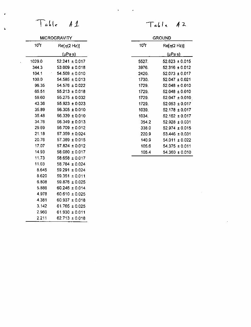
A. Appendix: Tablulated viscosity data
Table A1 and A2 give values of Re (r/) outside the viscoelastic region. Only data taken at 2
Hz are listed. The data at higher frequencies were consistent with those at 2 Hz; however,
they had smaller signal-to-noise ratios. Some of the values represent a single 45-minute
data point, and their uncertainty al was estimated as the standard deviation of all of the
33

45-minutepoints from a fit to the data in the range10-° < t < 10 -3. The other values are
averages of N 45-minute points, and their uncertainty was estimated as az/v/'N.
Table A3 gives values of Re (7) and Im (7) / Re (77) inside the viscoelastic region. Each
temperature represents a single 45-minute data point.
34
MICROGRAVITY
10St
1029.0
344.3
104.1
100.0
96.35
65.51
59.60
43.36
35.89
35.48
34.76
29.69
21.18
20.76
17.07
1493
11.73
11.03
8.645
8.620
6.808
5.886
4.978
4.381
3.142
2.960
2.211
ReIr/(2 Hz)]
(IJPa-s)
52.241 + 0.017
53.009 ± 0.018
54.509 + 0.010
54.585 ± 0.013
54.576 + 0.022
55.213 + 0.018
55.275 + 0.032
55.923 + 0.023
56.305 ± 0.010
56.339 + 0.010
56.349 ± 0.013
56.709 + 0.012
57.359 + 0.024
57.389 ± 0.015
57.824 + 0.012
58.080 + 0.017
58.658 + 0.017
58.784 + 0.024
59.291 + 0.024
59.351 + 0.011
59.876 + 0.025
60.246 ± 0.014
60.610 ± 0.025
60.937 + 0.018
61.765 + 0.025
61.930 ± 0.011
62.713 ± 0.018
GROUND
/r?..
10st
5527.
3976.
2420.
1730.
1729.
1729.
1729.
1729.
1039.
1034.
354.2
338.0
220.9
140.9
105.6
105.4
Re[r/(2 Hz)]
(pPa.s)
52.623 ± 0.015
52.316 ± 0.012
52.073 ± 0.017
52.047 ± 0.021
52.048 ± 0.010
52.048 ± 0.010
52.047 ± 0.010
52.053 ± 0.017
52.178 ± 0.017
52.162 ± 0.017
52.928 ± 0.031
52.974 ± 0.015
53.446 ± 0.031
54.011 ± 0.022
54.375 ± 0.011
54.360 ± 0.010

106t
2 Hz
+ 0.04
Re(o)/(mPa-s)
3 Hz 5 Hz 8 Hz 12 Hz
+0.04 +0.05 +0.07 +0.11
19.91 63.00 63.00 62.99 63.04 6292
18.91 63.14 63.13 63.12 63.09 62.94
16.63 63.46 63.47 63.41 63.51 63.47
15.70 63.62 63.64 63.63 63.60 63.55
13.80 63.96 63.97 63.99 63.91 63.95
12.72 64.18 64.18 64.17 64.23 63.93
11.92 64.33 64.36 64.36 64.37 64.19
11.03 64.53 64.53 64.50 64.50 64.36
t0.27 64.71 64.72 64.70 64.66 64.66
9.76 64.83 64.84 64.84 64.85 64.62
9.27 64.96 64.99 64.98 64.99 64.79
8.84 65.13 65.11 65.06 65.06 64.81
8.38 65.27 65.26 65.26 65.16 65.27
7.87 65,43 65.42 65.40 65.40 65.35
7.41 65.58 65.57 65.53 65.48 65.24
6.97 65.77 65.79 6570 65.71 65.57
6.21 66.09 66.08 66.05 65.95 65.83
5.34 66.47 66.49 66.38 66.41 66.11
4.88 66,77 66.74 66.68 66.63 66.56
4,40 67.00 67.01 66.93 66.90 66.43
3.95 67.31 67.30 67.28 67.12 66.81
3.49 67.64 67.60 67.46 67.25 67.11
3.02 68.00 67.95 67.81 67.59 67.45
2,60 68,37 68.25 68.17 67.93 67.51
2,19 68.82 68.74 68.53 68.19 67,58
1.69 69,38 69.24 68,92 68,56 68,22
128 69.94 69.71 69.39 68,85 68.60
0,79 70.65 70.33 69.81 69.36 68.68
0.31 71.43 70.98 70,39 69.71 69.05
-lO'lm(q)lRe(q)
2Hz 3Hz 5Hz 8Hz 12Hz
+8 +6 ±4 +8 ±15
5 9 7 17 11
6 8 -1 9 4
7 2 8 25 7
9 7 11 12 28
5 7 15 17 -13
-8 9 12 31 15
5 13 18 12 10
2 12 11 31 23
9 14 18 42 56
5 15 20 29 51
5 12 24 39 58
5 15 16 50 3
2 15 22 47 24
9 17 32 43 17
3 19 26 53 72
18 21 20 40 45
17 28 40 64 63
22 32 43 62 62
39 45 57 82 76
28 44 58 92 115
38 56 69 94 103
48 63 71 107 118
55 79 84 113 111
77 98 102 145 123
90 110 131 157 175
111 131 155 178 222
143 169 187 207 198
179 213 237 265 253
268 290 300 319 306

B. Appendix: Electrostriction
The relative increase in the density Ap/pc caused by a time-independent, electric field E is
p--:-= _ X_, (B.1)
where PE = (exe/e0 - 1)eoE2/2 is the induced change in chemical potential per unit mass,
Pc is xenon's critical pressure, and e0 and exe are the dielectric constants of vacuum and
xenon. Electrostriction is conspicuous near Tc because of the large density changes resulting
from the large value of X_, the reduced susceptibility at constant temperature.
As a first step toward calculating E, we ignored the oscillator's presence and modeled the
electric field between the viscometer's driving electrodes as that in a parallel plate capacitor.
See Figure 17. If the voltages on the two electrodes are 1/1 and V2, and the distances from
the oscillator to the two electrodes are xl and x2, this electric field is
Eo = (I/1 - 1/2) (B.2)(zl +
Electrostriction due to E0 was insignificant.
Next we modeled the field concentrated near one of the thin wires comprised by the
oscillator. We adapted Spangenberg's [39] model for the electric potential in a vacuum tube,
consisting of two electrodes and a grid modeled as planar array of parallel line charges. The
radial field Er near one of the wires, modeled as a cylinder, is
Er(r,O) = (El + f2) _ + E0 1 + cos(0). (B.3)
Here r and 0 are cylindrical coordinates centered on the wire, R is the radius of the wire,
and a >> R is the spacing between wires. The first term in Eq.(B.3) originates in the wire's
induced line charge, and it disappears when the fields El -- V1/xi and E2 - V2/z2 are equal
and opposite. It is a factor of two smaller than in Spangenberg's model because the charge
induced on the CVX oscillator was spread over transverse as well as longitudinal wires. The
second term originates in the wire's induced line dipole; it was added to Spangenberg's model
to create a zero potential surface at r = R.
37

We applied Eq.(B.3) to CVX using the valuesa = 0.85 mm, R = 0.009 ram, and
Vl = -V2 = VDC = 30 V. We allowed for asymmetry in the viscometer's construction by
estimating the unequal distances xl = 3 mm and x2 = 5 ram. At the wire's surface, the field
was concentrated by the factor E,-/Eo = 6. At Tc + 0.3 mK, the associated density increase
was only 0.05% and thus negligible.
C. Appendix: Frequency-dependent scaling function S (z)
Bhattacharjee and Ferrell calculated the frequency-dependent viscosity of a classical fluid
near its critical point. The relevant portion of their results in Reference [8] are reproduced
here, correcting two typographic errors in the original published expressions for In (5'4) and
for R (z).
The dependence of the viscosity on correlation length _ and frequency f is
(c.1)
where the argument of the scaling function S (z) is the scaled frequency defined by z =
--ilrfT. Bhattacharjee and Ferre]l used the decoupled-mode theory to calculate S(z) to
single-loop order. They accurately approximated their result in closed form by an average
of calculations in two and four dimensions.
Here, the tilde refers to additional rescalings given by
(C.2)
_ (z) = s_ ((2/e)' z) and
The scaling functions $2 and $4 are given by
S4 - S4 ((8/e) z) . (C3)
and
= + In z (c.4)
--z +_ lnz+ 5--+7 R(z), (C.5)
38
References
[1] P.C. Hohenberg and S.I. Halperin, Rev. Mod. Phys. 49, 435 (1977).
[2] M.R. Moldover, J.V. Sengers, R.W. Gammon, and R.J. Hocken, Rev. Mod. Phys. 51,
79 (1979).
[3] R.W. Gammon, J.N. Shaumeyer, M.E. Briggs, H. Boukari, D. Gent, and R.A. Wilkin-
son, page 137, Proceedings of the 1997 NASA/JPL Microgravity Fundamental Physics
Workshop, (NASA Document D-15677, JPL, Pasadena, CA) (1998).
[4] R.A. Wilkinson, G.A. Zimmerli, H. Hao, M.R. Moldover, R.F. Berg, W.L. Johnson,
R.A. Ferrell, and R.W. Gammon, Phys. Rev. E 57, 436 (1998).
[5] G.A. Zimmerli, R.A. Wilkinson, R.A. Ferrell, and M.R. Moldover, preprint (1998).
[6] J. Straub, A. Haupt, and L. Eicher, Int. J. Thermophys. 16, 1033 (1995).
[7] Y. Garrabos, B. Le Neindre, P. Guenoun, B. Khalil, and D. Beysens, Eurphys. Lett.
19, 491 (1992).
[8] J.K. Bhattacharjee and R.A. Ferrell, Phys. Rev. A 27, 1544 (1983).
[9] J.K. Bhattacharjee, R.A. Ferrell, R.S. Basu, and J.V. Sengers, Phys. Rev. A 24, 1469
(1981). (The crossover function from this reference is also summarized in Appendix A
of Reference [10].)
[10] R.F. Berg and M.R. Moldover, J. Chem. Phys. 93, 1926 (1990).
[11] L. Bruschi and hl. Santini, Phys. Lett. A 73, 395 (1979).
[12] L. Bruschi, II Nuovo Cimento 1D, 362 (1982).
41

[13] Y. Izumi, Y. Miyake, and R. Kono, Phys. Rev.A 23, 272 (1981).
[14] R.F. Bergand M.R. Moldover, J. Chem.Phys. 89, 3694(1988).
[15] H. Hao, R.A. Ferrell, and J.K. Bhattacharjee, preprint (1997). Hao et al. used the
value r/= 0.040 for the exponent r/that appears in the correlation function to obtain
z_ = 0.066. We used the value r/ = 0.035 (see [33, 34]) in their expressions to obtain
z, = 0.O67.
[16] R.A. Ferrell and J.K. Bhattacharjee, Phys. Rev. A 31, 1788 (1985).
[17] R.F. Berg and M.R. Moldover, Science Requirements Document, report to NASA Lewis
Research Center, 60009-DOC-006 (1993).
[18] A.M. Peddle, Flight instrument specification for the Critical Viscosity of Xenon flight
project, 60009-DOC-014 (1996).
[19] M.J. Assael, Z.A. Gallis, and V. Vosovic, High Temp. - High Press. 28, 583 (1996).
[20] In order to describe materials and experimental procedures adequately, it is occasion-
ally necessary to identify commercial products by manufacturer's name or label. In no
instance does such identification imply endorsement by the National Institute of Stan-
dards and Technology, nor does it imply that the particular product or equipment is
necessarily the best available for the purpose.
[21] R.F. Berg, Rev. Sci. Instrum. 66, 4665 (1995).
[22] R.F. Berg, G.A. Zimanerli, and M.R. Moldover, Int. J. Thermophys. 19, 481 (1998).
[23] D.W. Oxtoby, J. Chem. Phys. 62, 1463 (1975).
[24] I.S. Steinhart and S.R. ttart, Deep Sea Res. 15,497 (1968).
[25] V.A. Rabinovich, A.A. Vasserman, V.I. Nedostup, L.S. Veksler, Thermophysical Proper-
ties of Neon, Argon, Krypton, and Xenon (Hemisphere Publishing, Washington, 1987).
42

[26] R.F. Berg, M.J. Lyell, G.B. McFadden,and R.G. Rehm,Phys. Fluids 8, 1464(1996).
[27] R.F. Berg, Int. J. Thermophys.16, 1257(1995).
[28] R.E. Williams and R.G. Hussey,Phys. Fluids 11, 2083(1972).
[29] U. N//rger and D.A. Balzarini, Phys.Rev. B 42, 6651(1990).
[30] J. Luettmer-Strathmann, J.V. 8engers,and (].A. Olchowy,J. Chem. Phys. 103, 7482
(1995).
{31] J.V. Sengersand J. Luettmer-Strathmann, Chapter 6 in Transpor_ Properties of Fluids,
edited by J. Millat, J.H. Dymond, and C.A. Nieto de Castro (Cambridge University
Press, New York, 1996).
[32] J.V. Sengers, private communication (1998).
[33] H.W.J. B15te, E. Luijten, and J.R. Heringa, J. Phys. A: Math. Gen. 28, 6289 (1995).
[34] R. Guida and J. Zinn-Justin, Nucl. Phys. B 489 [FS], 626 (1997).
[35] H. Hao, R.A. Ferrell, and J.K. Bhattacharjee, preprint (1997).
[36] E.D. Siggia, B.I. Halperin, and P.C. Hohenberg, Phys. Rev. B 13, 2110 (1976).
[37] H. Giittinger and D.S. Cannell, Phys. Rev. A 24, 3188 (1981).
[38] J.K. Bhattacharjee and R.A. Ferrell, Phys. Lett. 27A, 290 (1980).
[39] K.R. Spangenberg, Vacuum Tubes (McGraw-Hill, New York, 1948).
[40] J.V. Sengers and M.R. Moldover, Phys. Lett. 66A, 44 (1978).
[41] R. Tofeu, B. Le Neindre, and P. Bury, Compte Rendus Acad. Sci. Paris B 273, 113
(1971).
43

E. Figures
1. Log-log plot of xenon's viscosity measured near the critical point. The asymptotic line
has the slope z_/v = 0.0435 deduced from the present microgravity data. Near To, the
CVX microgravity data (Re (r/) at 2 Hz) depart from the asymptotic line because of
viscoelasticity. The two sets of ground data depart from the asymptotic line further
from Tc because the xenon stratified in Earth's gravity.
2. Xenon's viscosity at critical density measured at frequencies from 2 to 12 Hz. The solid
curves resulted from fitting Eq.(1.2) to the data in the range 10 -6 < t < 10 -4. (a) The
real viscosity Re (r/). Near t = 10 -s, the data depart from the 0 Hz curve because of
viscoelasticity. (b) The ratio Im (r/)/Re (r/). For clarity, the ratio data at frequencies
above 2 Hz are displaced downward by integer multiples of 0.005; otherwise they would
coincide at t > 10 -s.
3. The temperature timeline followed by CVX. Both panels show the same data but with
different vertical scales.
4. Viscometer response as a function of temperature very near To. Both panels show data
at three ramp rates. On the lower panel, the temperature scale is expanded by a factor
of 8. (a) Above T_, data collected at the fastest ramp rate of -33 pK.s -1 reflect the
0.3% lower density caused by starting the ramp at Tc + 0.2 K. (b) Above T¢, data
collected while ramping at -0.05 /_K.s -l agree with those collected five days earlier
while ramping 20 times faster.
5. Cutaway view of the CVX viscometer cell. The cylindrical volume occupied by the
xenon was 38 mm long and 19 mm in diameter. Torque was applicd to the screen by
applying different voltages to diagonal pairs of electrodes while maintaining the screen
at ground potential.
44

6. The magnitude of the oscillator's transfer function measured in vacuum and in xenon
at critical density.
7. Cross-section of the Experimental cannister.
8. Simplified diagram of the circuit used to drive and detect the oscillator's motion.
9. The normalized density deviations calculated for a timeline similar to that used by
CVX. Each curve was calculated for at a radius r within a cylinder with isothermal
walls at radius Reel1.
10. The oscillator's transfer function Gme_ (f) in the frequency region used to determine
the viscosity.
11. Oscillations and spikes in the magnitude data at 1 Hz. The oscillation's 45-minute
period was half that of the Shuttle's orbital period. The minima of the oscillations
occurred when the Shuttle was near the Earth's equator. The three spikes indicated
by arrows occurred when the Shuttle was near the South Atlantic Anomaly.
12. Examples of the transfer function's magnitude measured at very low frequencies, where
noise was much greater in orbit than on Earth.
13. The calibration function B (R/_). The smooth curves indicate B (R/_5) calculated
from the hydrodynamic theory of a transversely oscillating circular cylinder of radius
R = 13.4/_m. (a) Magnitude scaled to reveal departures from the dominant (R/6) 3/2
behavior. (b) Phase.
14. The time dependence of the oscillator parameter ktr. The solid curve is a fit to the
transfer function's magnitude at 0.5 Hz, assuming that kt,. was a linear function of the
cell's temperature, the Experiment cannister's temperature, and time.
15. The transfer function's phase at 2 Hz as a function of time. The height of the boxes
corresponds to 0.2% of the density. The reproducibility of the oscillator's phase at 300
45

16.
17.
mK, 100mK, 30mK, and 3 mK aboveTc demonstrates that density deviations could
be reduced to within 0.1% of the average density at these temperatures. Filled points
were obtained below To. The points denoted "A" and "B" were obtained shortly after
warming the sample from below To. As discussed in the text, the equilibration of set
B was much slower than that of set A.
Cusps in the data very close to To. These data were taken at 5 Hz; similar features
occurred at other frequencies above 2 Hz. (a) Maximum damping (minimum ampli-
tude) of the oscillator occurred within 0.01 mK of T_, corresponding to t --- =[=3x 10 -_.
(b) A maximum of the phase located within 20 #K of To. The inset shows that the
maximum was superposed on a broader minimum.
Model cross section of the CVX electrodes used to calculate electric fields. The field
near the screen depended on the potentials Vl and V_, the distances xl, x2, and a, and
the wire radius R.
46

70
03
13_
6003o003
>
5O107
00
CVX
microgravity
high-Q oscillatorground []
z_ z3
CVX
ground
106 10s
asymptoticpower law
10 "4
t= (T-Tc) / Tc
1 0 -3
CVX calibration
at Tc+ 1 K
1 0 °2 10-1
1
Figure 1 lgOg.jnb

26
24
_ 22
° !_ 20.I calibration
18- I JL/ atTc+
1 K
," .',--_16 , , ,
0 1 2 3 4
16.9
! | I I I I !
5 6 7 8 9 10 11
16.8
OO
16.7
CLE
16.6
16.5
0
• -33 pK/s
m m _
-0.05 pK/si I I I I I I I I
2 3 4 5 6 7 8 9 100
11 12
Mission Elapsed Time / days
t C
12
m C

iI_ I (a)
04 -0.86 0
-0.90h __ I _ -_.oo,_s
-0.92 '_
16.570 16.575 16.580-0.88
N"i-04
-0.9003
t-"Q.
I
16.571
II
• -0.05 #K/s
[] -1.00 I_K/s
0 -33 i_K/s
16.572
(b)q
Temperature (°C)
Tc 1.jnb

o_"0
(1)i,.,
iim
r-Q.Q.

1000
(.-0
(3{.-
Q)cOc-
i.
0(1)
c-"
E
100
10
0.1
0.010.001
vacuum I
ixenon,1116 kg/m 3
(17 °C)0 o 0 00£
0
0
0
0o00
o
frequency / Hz
0.01 0.1 1 10 100

DEC 10 '12 09;32 FR HYMR 216 9?? _269 TO 913019694020 P.02/02
II
7

0
N
-I-
C_4
|
I
I
I
I
I
I
I
I
I
N
_11 : 5 1 I,
IJ° ,,,

0.005 I
r/Rcel I
°°°° [ _----7-- o.6" __ _ .
IV/ I ! I Tc+ 3mKli T,.+loomKI I To+10mK
-0.005 l _1_--__-_ I Tc + 30lmK I ,
4 5 6 7 8
time / days
rhovsT.jnb

"0-'I
o_
c-
E
o9c-
o9
[.-{3.
0.3
0.2
0.1
I I I I
0.0 I I I I I
0 2 4 6 8 100
-1
I
0 2
-2
I I I I
I I
4 6
frequency / Hz
! 1
12
8 10 12

0.308
i
Nt
0.304"I'-"
C
0.300E
0.296 {{5
Mission Elapsed Time / days
6

,-" 0.30
c-
coc-
0
"0
c-0')a_E
0.20.001
/ _ ground test
fhght
frequency / Hz
Iowfreq 1.jnb

3.3
3.2
53
.__. 3.1
3.0
2.90.0
30-
En
m 20 -CDI.,,
(_a/ o _ calculatedo measured
0
/1\_ / •
I I
0.1 0.2 0.3 0.4
(b)
calculated
° measuredo o
%0
10 I I I I
0.0 0.1 0.2 0.3 0.4
R/8
cylinder2.inb

N-r"LrJO
t-E_03E
0.302
0.300
0.298
0.296
o measured
modeled
[]
• [] # ' rl
8
0.294 I I I ! I I I I I I I0 1 2 3 4 5 6 7 8 9 10 11
Mission Elapsed Time / days
12
I
0.SHz.jnb

-0.78300 mK
100 mK
N-1-
c-O.
I
2
A
I I I I I 1 ....
3 4 5 6 7 8
Mission Elapsed Time / days
B
I
9 10
30 mK
3mK
mK
2Hz.jnb

NTLO
"O
(.-
E
N'r"It')
(Do3
c'-Q..
0.124
0.120
0.116
-1.8O
(a),II
B
o
I
16.571
I(b) :4
go
o °_°
°°o'_o_ e_+
_oo
o_ o • °
I
16.571
[]
[]
/ Tc "_o
vS'
EZ,_
[][]
single measurement
45-minute average
16.572 16.573
+1
, {
_,%.'."_"..:o I. _'°_, o ,, 16.57° _'_1.__,_,_oOoo o °
o °_a"-! oO_,o •8oo o '+""_o e,,,l_,_'U°O o
o _..,Zo°t-_o ",°° _'o:'.'°'_4__oI_'D [] [] []
° ° +% oo° q_'-'_o
0o o
0000000 OI
16.59
[] [][]
I
16.572
I
16.573
Cell temperature (°C)
5Hzslow.jnb

2R
"_''"_-"_'---', ' + 3 0 V
x2t
X 1
a
• • • OV


