
For Review Only
Differential Transformation Method for Vibration of
Membranes
Journal: Songklanakarin Journal of Science and Technology
Manuscript ID SJST-2017-0432.R1
Manuscript Type: Original Article
Date Submitted by the Author: 14-Feb-2018
Complete List of Authors: Mansilp, Kamonpad; King Mongkut's Institute of Technology Ladkrabang, mathematics Kasemsuwan, Jaipong; King Mongkut's Institute of Technology Ladkrabang, mathematics
Keyword: Vibration of Membrane, Differential Transformation Method, Analytical Solution, Approximate Solution.
For Proof Read only
Songklanakarin Journal of Science and Technology SJST-2017-0432.R1 Mansilp
For Review Only
DIFFERENTIAL TRANSFORMATION METHOD FOR VIBRATION OF
MEMBRANES
Original Article
Kamonpad Mansilp1*, and Jaipong Kasemsuwan
2
1,2Department of Mathematics, Faculty of Science,
King Mongkut's Institute of Technology Ladkrabang,
Bangkok 10520, Thailand.
* Corresponding author, Email address: [email protected]
Abstract
The purpose of this research is to apply the three-dimensional differential transform
method to estimate solutions to the equation of motion for vibration in a membrane with
certain boundary condition problems. The analytical solutions without an external force and
damping term under the initial and boundary conditions are presented. We found that the
comparison results between the analytical solution and the estimated solution are in good
agreement in case of no damping and the external force. Furthermore, the differential
transform method can be used to find approximated solutions taking into account both an
external force and damping term. This cannot be achieved via an analytical solution.
2010 Mathematics Subject Classification: 35G20, 35L05, 35L10 , 35L70.
Keywords: Vibration of Membrane, Differential Transformation Method, Analytical
Solution, Approximate Solution.
Page 3 of 30
For Proof Read only
Songklanakarin Journal of Science and Technology SJST-2017-0432.R1 Mansilp
123456789101112131415161718192021222324252627282930313233343536373839404142434445464748495051525354555657585960

For Review Only
1. Introduction
Many researchers have attempted to understand several phenomena occurring in
nature by applying knowledge from different field such as mechanical engineering, electrical
engineering, industrial engineering, energy and medicine. Most of these problems have been
studied by employing some form of mathematical modeling using both ordinary differential
equation (ODE) and partial differential equation (PDE). These problems require an accurate
solution, either as an analytical solution or approximate solution. The differential transform
method (DTM) is among the most effective mathematical methods for finding solutions to
these differential equations (Hatami, Ganji, & Sheikholeslami, 2017).
The differential transform method (DTM) is based on the high-order Taylor series
expansion. This method is a powerful tool for solving linear and non-linear ordinary
differential equations (Ayaz, 2004; Arikoglu, & Ozkol, 2006; Catal, 2008) and for solving
two-and three-dimensionals partial differential equations in both linear and non-linear
problems. DTM can be used to solve the differential equation subject to initial and boundary
conditions having both linear and non-linear terms within an acceptable error range.
The two-dimensional differential transform method (2D-DTM) is used to find the
solutions of both linear PDEs (Chen & Ho, 1999; Othman, & Mahdy, 2010; Ayaz, 2003;
Yang, Liu, & Bai, 2006) and nonlinear PDEs (Bildik, Konuralp, Bek, & Kucukarslan, 2006;
Kangalgil & Ayaz, 2009; Biazar & Eslami, 2010; Biazar, Eslami, & Islam, 2012).
Additionally, the three-dimensional differential transform method (3D-DTM) is
applied to find the solutions of linear and non-linear PDEs (Saravanan & Magesh, 2013;
Bagheri & Manafianheris, 2012). It is noted that the differential transform method can be
used to solve multidimensional PDEs such as the Westervelt equation (Jafari, Sadeghi, &
Biswas, 2012), heat-like and wave-like equations (Tabaei, Celuk, & Tabaei, 2012), and fuzzy
Page 4 of 30
For Proof Read only
Songklanakarin Journal of Science and Technology SJST-2017-0432.R1 Mansilp
123456789101112131415161718192021222324252627282930313233343536373839404142434445464748495051525354555657585960

For Review Only
partial differential equations (Mirzaee & Yari, 2015) as well as the linear and nonlinear
system of PDEs (Ayaz, 2004; Zedan & AliAlghamdi, 2012).
Many researchers are concerned with the use of non-linear PDEs by applying several
transform methods as follows. The Fitzhuah Nangumo (FN) equation is a mathematical
model for solving scientific and engineering problems by using q-HATM and the fractional
reduced differential transform method (FRDTM) which is based on DTM (Kumar, Singh, &
Baleanu, 2017).
The numerical solutions to non-linear fractional dynamical model of interpersonal and
romantic relationships are presented by applying q-homotopy analysis via the Sumudu
transform method (q-HASTM) (Singh, Kumar, Qurashi, & Baleanu, 2017).
Jeffery-Hamel flow in non-parallel walls, which relates to non-linear PDE and occurs
in fluid dynamics and other scientific applications, is solved by using an efficient hybrid
computational technique, the homotopy analysis transform method (HATM) (Singh, Rashidi,
Sushila, & Kumar, 2017).
The homotopy perturbation Sumudu transform method (HPSTM) and homotopy
analysis Sumuda transform method (HASTM) are more convenient than the homotopy
perturbation method (HPM) and the homotopy analysis method (HAM) since they produce a
comparative analytical study for a system of time factional non-linear differential equations
(Choi, Kumar, Singh, & Swroop, 2016).
Further examples of the application of PDEs by Laplace transform method to various
problem include Case I-application of drum head vibration solving by separation of variables
method, and Case II and III-application of signal transmission and application of chemical
communication in insects. All three cases give simulations on the solutions implemented by
MATLAB software (Ojwando, 2016).
Page 5 of 30
For Proof Read only
Songklanakarin Journal of Science and Technology SJST-2017-0432.R1 Mansilp
123456789101112131415161718192021222324252627282930313233343536373839404142434445464748495051525354555657585960
For Review Only
A modified He-Laplace method (MHLM) is applied to solve space and time nonlinear
fractional differential-difference equations (NFDDEs) (Prakash, Kothandapan, & Bharathi,
2016).
In our previous work, we studied the suspended vibrating string equation using 2D –
DTM. It was found that DTM can be applied to various problems of the suspended string
equation.
In this proposed work, we study further the vibration equation in three dimensions of
the motion of a membrane using the 3D-DTM. The oscillation of a membrane-like plate,
which is determined by the tension and insignificant resistance to the bending. The
differential transform method was applied to find solutions of the motion equation of a
membrane with an external force and damping term. We compare the results with an
analytical solution. We show in detail the derivation of the transformed formula of DTM
which is of the nth power form (to be shown in theorem 3.6). The obtained formula helps
simplify the use of DTM in solving non-linear PDEs. It is noted that the formula requires
high computation to find a complete solutions mainly due to the fact that the formula is in the
recursive form.
The equation of motion of a membrane
The equation of motion for the forced transverse vibration of a membrane, after (Rao,
2011) is as follows:
2 2 2
2 2 2( , , ) ( , ) ,
w w wP f x y t x y
x y tρ
∂ ∂ ∂+ + = ∂ ∂ ∂
(1)
where ( , , )f x y t is the pressure acting in the z direction(external force), P is the intensity of
tension at a point equal to production of the tensile stress and the thickness of the membrane,
Page 6 of 30
For Proof Read only
Songklanakarin Journal of Science and Technology SJST-2017-0432.R1 Mansilp
123456789101112131415161718192021222324252627282930313233343536373839404142434445464748495051525354555657585960

For Review Only
and ( , )x yρ is the mass per unit area. We assume that ( , , ) 0f x y t = , 1,P = and ( , ) 1.x yρ =
Then Eq.(1) leads to:
2 2 2
2 2 2.
w w w
x y t
∂ ∂ ∂+ =
∂ ∂ ∂
(2)
The initial conditions of (2) after (Rao, 2011) are:
( , ,0) sin sin , 0 , 0 ,
( , ,0) 0, 0 , 0 ,
x yw x y x a y b
a b
wx y x a y b
t
π π= ≤ ≤ ≤ ≤
∂= ≤ ≤ ≤ ≤
∂
we assumed that 1a = and 1b = .Therefore, the boundary conditions of the equation of motion
of a membrane are definded thus:
( ,0, ) 0, 0 1,
(0, , ) 0, 0 1,
( ,1, ) 0, 0 1,
(1, , ) 0, 0 1, .
w x t x
w y t y
w x t x
w y t y t
= ≤ ≤
= ≤ ≤
= ≤ ≤
= ≤ ≤ ∈�
(3)
An analytical solution
The following is the derivation of the analytical solution of the problem (2).
Considering the initial conditions ( , ,0) sin sinw x y x yπ π= and ( , ,0) 0,w
x yt
∂=
∂ the boundary
conditions are shown in (3).The general solution can be derived by the separation of variables
technique:
( , , ) ( ) ( ) ( ),w x y t X x Y y T t= (4)
Subject to the eigenvalue, 2 2,ω α− and
2β , can be written (2)
2( ) ( ) ( ),
( ) ( ) ( )
X x Y y T t
X x Y y T tω
′′ ′′ ′′+ = = −
2( ) ( ),
( ) ( )
X x Y y
X x Y yω
′′ ′′+ = −
Page 7 of 30
For Proof Read only
Songklanakarin Journal of Science and Technology SJST-2017-0432.R1 Mansilp
123456789101112131415161718192021222324252627282930313233343536373839404142434445464748495051525354555657585960
For Review Only
and
2 2( ) ( ),
( ) ( )
X x Y y
X x Y yω α
′′ ′′− = + =
2( ),
( )
X x
X xα
′′− =
then 2( ) ( ) 0,X x X xα′′ + =
2 2( ),
( )
Y y
Y yα ω
′′= −
assumed 2 2 2 ,α ω β− + = 2 2( ) ( ) ( ) 0,Y y Y yα ω′′ + − + =
then 2( ) ( ) 0,Y y Y yβ′′ + =
and
2( ),
( )
T t
T tω
′′=
then 2( ) ( ) 0,T t T tω′′ + =
2( ) ( ) 0,X x X xα′′ + = (5)
2( ) ( ) 0Y y Y yβ′′ + = , (6)
2( ) ( ) 0.T t T tω′′ + = (7)
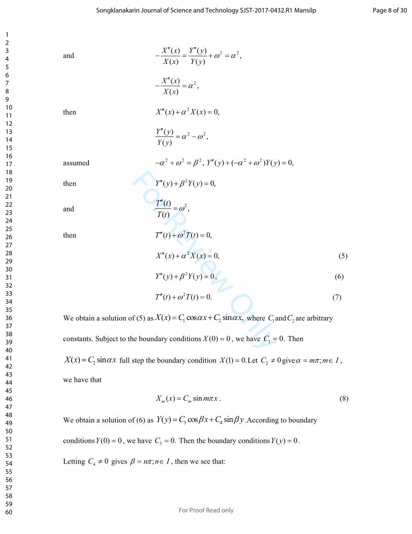
We obtain a solution of (5) as 1 2( ) cos sin ,X x C x C xα α= + where 1C and 2C are arbitrary
constants. Subject to the boundary conditions (0) 0X = , we have 1 0.C = Then
2( ) sinX x C xα= full step the boundary condition (1) 0.X = Let 2 0C ≠ give ;m m Iα π= ∈ ,
we have that
( ) sinm mX x C m xπ= . (8)
We obtain a solution of (6) as 3 4( ) cos sinY y C x C yβ β= + .According to boundary
conditions (0) 0Y = , we have 3 0.C = Then the boundary conditions ( ) 0Y y = .
Letting 4 0C ≠ gives ;n n Iβ π= ∈ , then we see that:
Page 8 of 30
For Proof Read only
Songklanakarin Journal of Science and Technology SJST-2017-0432.R1 Mansilp
123456789101112131415161718192021222324252627282930313233343536373839404142434445464748495051525354555657585960

For Review Only
( ) sin .n nY y C n yπ= (9)
From
2 2 2
2 2
,
.m n
ω β α
ω π
= +
= +
We obtain a solution of (7) as
( ) cos sinmn mn mnT t A t B tω ω= + .
Then
2 2 2 2( ) cos sinmn mn mnT t A m n t B m n tπ π= + + + . (10)
According to (8), (9) and (10) can be written
( )( )
2 2
2 2
( , , ) ( ) ( ) ( ),
sin sin cos
sin sin sin ,
mn
mn m n
mn m n
W x y t X x Y y T t
A C C m x n y m n t
B C C m x n y m n t
π π π
π π π
=
= +
+ +
(11)
where mn mn m nF A C C= , mn mn m nH B C C= and for all ,m n I∈
By using the superposition principle (11) become
( )( )
1 1
2 2
1 1
2 2
( , , ) ( , , ),
sin sin cos ,
sin sin sin .
mn
m n
mn
m n
mn
w x y t w x y t
F m x n y m n t
H m x n y m n t
π π π
π π π
∞ ∞
= =
∞ ∞
= =
=
= +
+ +
∑∑
∑∑ (12)
According to the initial condition ( , ,0) sin sinw x y x yπ π= and ( , ,0) 0.w
x yt
∂=
∂ By using
Fourier series, we have
1 ; 1 1,
0; ,
2 .
mn
mn
F m and n
H m n I
ω π
= = =
= ∈
=
Substituting 11 1F = , 0mnH = and 2ω π=
in (12), we obtain the analytical solution:
Page 9 of 30
For Proof Read only
Songklanakarin Journal of Science and Technology SJST-2017-0432.R1 Mansilp
123456789101112131415161718192021222324252627282930313233343536373839404142434445464748495051525354555657585960

For Review Only
( , , ) sin sin cos 2 .w x y t x y tπ π π= (13)
In the case of the problem (2) with damping term are represented by
2 2 2
2 2 2.
w w w w
t x y t
∂ ∂ ∂ ∂= + −
∂ ∂ ∂ ∂
By similar calculation, we obtain the solution of , ( )m nT t as
2 2
2, , ,
1 4 1 4( ) ( cos sin )
2 2
t
m n m n m nT t e A t B tω ω− − −
= + . (14)
Considering (14), we can see that substituting 2ω π=
to (14), it make 21 4ω− be the
complex number. Therefore ( )T t are not solvable.
2. Three-Dimensional Differential transform method
The basic definitions and fundamental operations of differential transform are defined
below.
Definition 2.1 The three-dimensional differential transform of function ( , , )w x y t is defined
as:
(0,0,0)
1 ( , , )( , , )
! ! !
k h m
k h m
w x y tW k h m
k h m x y t
+ +∂=
∂ ∂ ∂0, 0 0.k h and m≥ ≥ ≥
Definition 2.2 The inverse three-dimensional differential transform of sequence
{ }, , 0
( , , )k h m
W k h m∞
=is defined as:
0 0 0
( , , ) ( , , ) .k h m
k h m
w x y t W k h m x y t∞ ∞ ∞
= = =
= ∑∑∑
(14)
Page 10 of 30
For Proof Read only
Songklanakarin Journal of Science and Technology SJST-2017-0432.R1 Mansilp
123456789101112131415161718192021222324252627282930313233343536373839404142434445464748495051525354555657585960

For Review Only
3. The fundamental operations of three-dimensional differential transform method .
From Table 1 theorem 3.1-3.5 shown in (Yang, Liu, & Bai, 2006).
The following is the derivation of theorem 3.6:
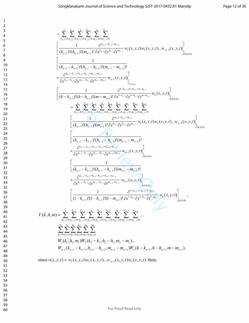
If 1 2 1( , , ) ( , , ) ( , , )... ( , , ) ( , , )n nv x y t w x y t w x y t w x y t w x y t−= then,
1 1 1 3 13 32 2 2
1 2 1 2 1 2 2 1 2 1 2 10 0 0 0 0 0 0 0 0 0 0 0
1 1 1 1 2 2 1 2 1 2 1
1 1 2 1 2 1 2 1 1
( , , ) ...
( , , ) ( , , )...
( , , ) ( , ,
n n n
n n n n n n
mk h m k h mk hk h m
k k h h m m k k h h m m
n n n n n n n n n n
V k h m
W k h m W k k h h m m
W k k h h m m W k k h h
− − −
− − − − − −= = = = = = = = = = = =
− − − − − − − − −
=
− − −
− − − − −
∑ ∑ ∑ ∑ ∑ ∑ ∑∑∑∑ ∑ ∑
1 ).nm m −−
For : , : ; , : , : ; ,n nV I W I n I v w n I x+ + + +→ → ∈ → → ∈ ∈� � � � � � �
and , , 0,1,2,3,...k h m =
By definition of the three-dimensional differential transform:
(0,0,0)
1 ( , , )( , , ) ,
! ! !
k h m
k h m
v x y tV k h m
k h m x y t
+ + ∂= ∂ ∂ ∂
we obtain 1 2 1( , , ) ( , , ) ( , , )... ( , , ) ( , , )n nv x y t w x y t w x y t w x y t w x y t−=
Then by using definition (13), we have:
1 1 1
1 1 1
1 1
1 2 1
(0,0,0)
0 0 0 1 1 1 1 1 1
1( , , ) ( , , ) ( , , )... ( , , ) ( , , )
! ! !
1 ! ! !
! ! ! ( )!( )! ( )!( )! ( )!( )!n n n
n n n
n n
k h m
n nk h m
k h m
k h m n n n n n n
k h m
k h
V k h m w x y t w x y t w x y t w x y tk h m x y t
k h m
k h m k k k h h h m m m
x y t
− − −
− − −
− −
+ +
−
= = = − − − − − −
+ +
∂= ∂ ∂ ∂
=− − −
∂
∂ ∂ ∂
∑ ∑ ∑
1
1 1 1
1 1 1
1 2
1
(0,0,0)
( , , ) ( , , )...
( , , ) ( , , )
n
n n n
n n n
m
k k h h m m
n nk k h h m m
w x y t w x y t
w x y t w x y tx y t
−
− − −
− − −
− + − + −
− − − −
∂∂ ∂ ∂
1 1 1
1 1 1
1 1 1
1 1 1
1 1 1
0 0 0
1 2 1
1 1 1 (0,0,0)
1 1 1
1( , , ) ( , , )... ( , , )
( )!( )!( )!
1
( )!( )!( )!
n n n
n n n
n n n
n n n
n n n
k h m
k h m
k h m
nk h m
n n n
k k h h m m
nk k h h m m
n n n
w x y t w x y t w x y tk h m x y t
wk k h h m m x y t
− − −
− − −
− − −
− − −
− − −
= = =
+ +
−− − −
− + − + −
− − −− − −
=
∂ ∂ ∂ ∂
∂− − − ∂ ∂ ∂
∑ ∑ ∑
(0,0,0)
( , , )x y t
Page 11 of 30
For Proof Read only
Songklanakarin Journal of Science and Technology SJST-2017-0432.R1 Mansilp
123456789101112131415161718192021222324252627282930313233343536373839404142434445464748495051525354555657585960
For Review Only
1 1 1
1 2 1 2 1 2
2 2 2
2 2 2
0 0 0 0 0 0
1 2 2
2 2 2 (0,0,0)
1 2 1 2 1 2
1( , , ) ( , , )... ( , , )
( )!( )!( )!
1
( )!( )!( )!
n n n
n n n n n n
n n n
n n n
k h mk h m
k k h h m m
k h m
nk h m
n n n
n n n n n n
w x y t w x y t w x y tk h m x y t
k k h h m m
− − −
− − − − − −
− − −
− − −
= = = = = =
+ +
−− − −
− − − − − −
=
∂ ∂ ∂ ∂
− − −
∂×
∑ ∑ ∑ ∑ ∑ ∑
1 2 1 2 1 2
1 2 1 2 1 2
(0,0 ,0)
1 1 1
1 1 1
1
1 1 1 (0,0,0)
( , , )
1( , , )
( )!( )!( )!
n n n n n n
n n n n n n
n n n
n n n
k k h h m m
nk k h h m m
k k h h m m
nk k h h m m
n n n
w x y tx y t
w x y tk k h h m m x y t
− − − − − −
− − − − − −
− − −
− − −
− + − + −
−− − −
− + − + −
− − −− − −
∂ ∂ ∂
∂ − − − ∂ ∂ ∂
1 2 1 2 1 2
1 2 3 1 2 3 1 2 3
2 2 2
2 2 2
0 0 0 0 0 0 0 0 0
1 2 3
3 3 3 (0,0,0)
2
1( , , ) ( , , )... ( , , )
( )!( )!( )!
1
(
n n n n n n
n n n n n n n n n
n n n
n n n
k k h h m mk h m
k k k h h h m m m
k h m
nk h m
n n n
n n
w x y t w x y t w x y tk h m x y t
k k
− − − − − −
− − − − − − − − −
− − −
− − −
= = = = = = = = =
+ +
−− − −
−
=
∂ ∂ ∂ ∂
−
∑ ∑ ∑ ∑ ∑ ∑ ∑ ∑ ∑
2 3 2 3 2 3
2 3 2 3 2 3
1 2 1 2 1 2
1 2
3 2 3 2 3
2
(0,0,0)
1 2 1 2 1 2
)!( )!( )!
( , , )
1
( )!( )!( )!
n n n n n n
n n n n n n
n n n n n n
n n
n n n n
k k h h m m
nk k h h m m
n n n n n n
k k h h m m
k k
h h m m
w x y tx y t
k k h h m m
x y
− − − − − −
− − − − − −
− − − − − −
− −
− − − − −
− + − + −
−− − −
− − − − − −
− + − + −
−
− −
∂× ∂ ∂ ∂
− − −
∂×∂ ∂ 1 2 1 2
1 1 1
1 1 1
1
(0,0,0)
1 1 1
1 1 1
1 1 1 (0,0,0)
( , , )
1( , , ) ,
(1 )!(1 )!(1 )!
n n n n
n n n
n n n
nh h m m
k h m
nk h m
n n n
w x y tt
w x y tk h m x y t
− − − −
− − −
− − −
−− −
− + − + −
− − −− − −
∂
∂ − − − ∂ ∂ ∂
1 2 1 2 1 2
1 2 3 1 2 3 1 2 3
3 13 34 4 4
3 2 3 2 3 2
0 0 0 0 0 0 0 0 0
0 0 0 0 0 0
1 1 1 1 2 2 1 2 1 2 1
1 1 2 1
( , , ) ...
( , , ) ( , , )...
( ,
n n n n n n
n n n n n n n n n
k k h h m mk h m
k k k h h h m m m
k h mk h m
k k h h m m
n n n n
V k h m
W k h m W k k h h m m
W k k h
− − − − − −
− − − − − − − − −= = = = = = = = =
= = = = = =
− − − −
=
− − −
−
∑ ∑ ∑ ∑ ∑ ∑ ∑ ∑ ∑
∑∑∑∑ ∑ ∑
2 1 2 1 1 1, ) ( , , ).n n n n n n nh m m W k k h h m m− − − − − −− − − − −
since 1 2 1( , , ) ( , , ) ( , , )... ( , , ) ( , , )n nv x y t w x y t w x y t w x y t w x y t−= then,
Page 12 of 30
For Proof Read only
Songklanakarin Journal of Science and Technology SJST-2017-0432.R1 Mansilp
123456789101112131415161718192021222324252627282930313233343536373839404142434445464748495051525354555657585960
For Review Only
1 1 1 3 13 32 2 2
1 2 1 2 1 2 2 1 2 1 2 10 0 0 0 0 0 0 0 0 0 0 0
1 1 1 1 2 2 1 2 1 2 1
1 1 2 1 2 1 2 1 1
( , , ) ...
( , , ) ( , , )...
( , , ) ( , ,
n n n
n n n n n n
mk h m k h mk hk h m
k k h h m m k k h h m m
n n n n n n n n n n
V k h m
W k h m W k k h h m m
W k k h h m m W k k h h
− − −
− − − − − −= = = = = = = = = = = =
− − − − − − − − −
=
− − −
− − − − −
∑ ∑ ∑ ∑ ∑ ∑ ∑∑∑∑ ∑ ∑
1 ).nm m −−
4. Application
In this section, we apply the three-dimensional differential transform method to the
vibration of a membrane. We demonstrate four examples of the problem under different
conditions. The conditions are (i) without damping term, (ii) with damping term, (iii) with
external force, and (iv) with damping term and external force. The initial and boundary
conditions as defined as follows.
Example 4.1 Considering the equation of the motion for the vibration of a membrane
2 2 2
2 2 2,
w w w
t x y
∂ ∂ ∂= +
∂ ∂ ∂ (15)
with the initial and boundary conditions,
( , ,0) sin sin , 0 1, 0 1,
( , ,0) 0, 0 1, 0 1,
x yw x y x y
a b
wx y x y
t
π π= ≤ ≤ ≤ ≤
∂= ≤ ≤ ≤ ≤
∂
,
( ,0, ) 0, 0 1,
(0, , ) 0, 0 1,
( ,1, ) 0, 0 1,
(1, , ) 0, 0 1, .
w x t x
w y t y
w x t x
w y t y t
= ≤ ≤
= ≤ ≤
= ≤ ≤
= ≤ ≤ ∈�
(16)
Comparing (15) to the general terms of PDEs in Table 1, we have:
( , , ) ( , . ) ( , , ) 1.a x y t b x y t c x y t= = =
Then for all 0, 0i j≥ ≥ and 0,r ≥ we have
( , , ) ( , , ) ( , , ) ( , , ).A i j r B i j r C i j r i j rδ= = =
The following Kronecker symbols can be used:
Page 13 of 30
For Proof Read only
Songklanakarin Journal of Science and Technology SJST-2017-0432.R1 Mansilp
123456789101112131415161718192021222324252627282930313233343536373839404142434445464748495051525354555657585960
For Review Only
1; 0( , , ) ( ) ( ) ( ) ( , ) ( ) ( ).
0; ,
x y tx y t x y t x y x y
otherwiseδ δ δ δ δ δ δ
= = == = =
By applying DTM and Kronecker symbols to the given equation of motion for the vibration
of a membrane, we have
]
0 0 0
0 0 0
1( , , 2)
( 2)( 1) (0,0,0)
( 2)( 1) ( , , ) ( 2, , )
( 2)( 1) ( , , ) ( , 2, ) ,
1( 2)( 1)( 2)( 1) ( 2, , ) ( , 2, ),
( 2)( 1)
k h m
i j r
k h m
i j r
W k h mm m
k i k i A i j r W k i h j m r
h i h i B i j r U k i h j m r
k k h h W k h m W k h mm m
δ
= = =
= = =
+ =+ +
× − + − + − + − −
+ − + − + − − + −
+ + + + + ++ +
∑∑∑
∑∑∑
that is
[ ]( , , 2) ( 2)( 1)( 2)( 1) ( 2, , ) ( , 2, ) /
( 2)( 1)( 2)( 1).
W k h m k k h h W k h m W k h m
m m m m
+ = + + + + + +
+ + + + (17)
Comparing between the coefficient of Taylor’s series of sine and the series in the definition
(14)
2 4 6 8 10 123 5 7 9 112 4 6 8 10 12
sin( )sin( ) ...2! 4! 6! 8! 10! 12!
x y xt x t x t x t x t x tπ π π π π π
π π ≅ − + − + − +
0 0 2
0 0
3 2
2 2
( , ,0) (0,0,0) (1,1,0) (2,1,0)
(3,1,0) ... (0,1,0) (1,2,0)
(2,2,0) ...
k h
k h
W k h x y W x y W xy W x y
W x y W xy W xy
W x y
∞ ∞
= =
= + +
+ + + +
+ +
∑∑ (18)
Then, we have
0 0,1,2,... 0,2,4,6,...
( )( , ,0) 1,5,9,... 1,3,5,7,...
( )!
( )3,7,11,.. 1,3,5,7,...
( )!
k h
k h
if k and h
k hU k h if k and h
k h
k hif k and h
k h
π
π
+
+
= = +
= = =+
− += =
+
, (19)
Page 14 of 30
For Proof Read only
Songklanakarin Journal of Science and Technology SJST-2017-0432.R1 Mansilp
123456789101112131415161718192021222324252627282930313233343536373839404142434445464748495051525354555657585960
For Review Only
and from the initial condition (16)
( , ,1) 0, , 0,1, 2,3,...W k h k h= = , (20)
and from the boundary condition (16), we have
( ,0, ) 0, , 0,1,2,3,...,
(0, , ) 0, , 0,1,2,3,...,
( ,1, ) 0, , 0,1, 2,3,...,
(1, , ) 0, , 0,1, 2,3,...,
W k m k m
W h m h m
W k m k m
W h m h m
= =
= =
= =
= =
(21)
for each , ,k h m substituting(19)-(21) and by recursive method of (17), we obtain the
coefficients ( , , )W k h m for the series solution.
That is
2 4 2 6 4 8 6 4 3 6 2 31 1( , , ) .
1 1.
6 0 6.
9 6xy t xy t xy t xy x yu x y t t x yπ π π π π π− + −= +− +
As the result in (14), we can not apply the separation of variables technique to find the
analytical solution to the problem with damping term as equation (22). In the following
example, we apply the DTM to find the approximate solution to the problem.
Example 4.2 Considering the equation of motion for the vibration of a membrane with
damping term.
2 2 2
2 2 2,
w w w w
tt x y
∂ ∂ ∂ ∂= + −
∂∂ ∂ ∂ (22)
comparing (22) to general terms of PDEs in table 1, we have
( , , ) ( , . ) ( , , ) 1, ( , , ) 1.a x y t b x y t c x y t d x y t= = = = −
Then for all 0, 0i j≥ ≥ and 0,r ≥ we have
( , , ) ( , , ) ( , , ) ( , , ), ( , , ) ( , , ).A i j r B i j r C i j r i j r D i j r i j rδ δ= = = = −
By applying DTM and Kronecker symbols to the given equation of motion for the vibration
of a membrane, we have:
Page 15 of 30
For Proof Read only
Songklanakarin Journal of Science and Technology SJST-2017-0432.R1 Mansilp
123456789101112131415161718192021222324252627282930313233343536373839404142434445464748495051525354555657585960

For Review Only
[]
( , , 2) ( 2)( 1)( 2)( 1) ( 2, , ) ( , 2, )
( 1) ( , 1, ) / ( 2)( 1).
W k h m k k h h W k h m W k h m
h W k h m m m
+ = + + + + + +
− + + + + (23)
For each , ,k h m substituting(19)-(21) and by recursive method of (23), we obtain the
coefficients ( , , )W k h m for the series solution.
That is
2 2 6 4 4 2 3 6 4 3 6 2 5 8 4 55 5 5 5 1 1( , , ) ...
2 6 12 36 48 144w x y t t x t x t x t x t x t xπ π π π π π= − + + − − + +
Example 4.3 Considering the equation of motion for the vibration of a membrane with
external force.
2 2 23
2 2 2.
w w ww
t x y
∂ ∂ ∂= + −
∂ ∂ ∂ (24)
Comparing (24) to general terms of PDEs in table 1, we have:
( , , ) ( , . ) ( , , ) 1, ( , , ) 1.a x y t b x y t c x y t q x y t= = = = −
Then for all 0, 0i j≥ ≥ and 0,r ≥ we have:
( , , ) ( , , ) ( , , ) ( , , ), ( , , ) ( , , ).A i j r B i j r C i j r i j r Q i j r i j rδ δ= = = = −
By applying DTM and Kronecker symbols to the given equation of motion for the vibration
of a membrane, we have
[
]
2 2 2
2 1 2 1 2 1
1 1 1 1
0 0 0 0 0 0
2 2 1 2 1 2 1 3 2 2 2
( , , 2) ( 2)( 1)( 2)( 1) ( 2
( , , )
( , , )
, , ) ( , 2, )
( 2)( 1)( / ., , )
k h mk h m
k k h h m m
W k h m
W k k h h m m W
W k h m k k h h W k h m W k h m
m mk k h h m m
= = = = = =
+ = + + + +
−
+ +
+− − − − +−
−∑∑∑∑∑∑ (25)
For each , ,k h m substituting (19)-(21) and by recursive method of (25), we obtain the
coefficients ( , , )W k h m for the series solution.
That is:
8 8 102 4 2 6 4 6 4 3 6 2 31 1 1 1
( 3( ))6 30 6 18 36 6 6
( , , ) ...xy t xy t xy t xy x yw x y t x ytπ π π
π π π π π− + + − + − + +− −=
Page 16 of 30
For Proof Read only
Songklanakarin Journal of Science and Technology SJST-2017-0432.R1 Mansilp
123456789101112131415161718192021222324252627282930313233343536373839404142434445464748495051525354555657585960

For Review Only
Example 4.4 Considering the equation of the motion for the vibration of a membrane
with external force and damping term.
2 2 23
2 2 2.
w w w ww
tt x y
∂ ∂ ∂ ∂= + − −
∂∂ ∂ ∂
(26)
Comparing (26) to general terms of PDEs in table 1, we have
( , , ) ( , . ) ( , , ) 1, ( , , ) ( , , ) 1.a x y t b x y t c x y t d x y t q x y t= = = = = −
Then for all 0, 0i j≥ ≥ and 0,r ≥ we have
( , , ) ( , , ) ( , , ) ( , , ), ( , , ) ( , , ) ( , , ).A i j r B i j r C i j r i j r D i j r Q i j r i j rδ δ= = = = = −
By applying DTM and Kronecker symbols to the given equation of motion for the vibration
of a membrane, we have:
[
]
2 2 2
2 1 2 1 2 1
1 1 1 1 2 2 1 2 1 2 1
0 0 0 0 0 0
3 2 2 2
( , , 2) ( 2)( 1)( 2)( 1) ( 2, , ) ( ,
( , , ) ( , , )
( ,
2, )
(
,
1) ( , 1, )
) / ( 2)( 1).
k h mk h m
k k h h m m
W k h m k k h h W k h m W k h m
h W k h
W k h m W k k h h
m
m
m m
W k k mh h m m
= = = = = =
− − −
− − −
+ = + + + + + +
− + +
+ +
−∑∑∑∑∑∑ (27)
For each , ,k h m substituting (19)-(21) and by recursive method of (27), we obtain the
coefficients ( , , )W k h m for the series solution.
That is:
6 4
2 2 4 4 6 6 4 2 3 6 4 33 21 1 1 1 1
1/ 6 ( ( ) ( 2 ))2 30 12 12
(3
, , ) .6
..t x t x t xw x y t tt x xπ π π π π π π= +− + + − ++ − −
5. Results and Discussion
Next, we will show the results from examples 4.1 to– 4.4.
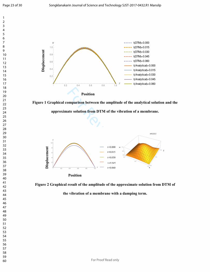
Figure 1 Graphical comparison between the amplitude of the analytical solution and the
approximate solution from DTM of the vibration of a membrane.
Page 17 of 30
For Proof Read only
Songklanakarin Journal of Science and Technology SJST-2017-0432.R1 Mansilp
123456789101112131415161718192021222324252627282930313233343536373839404142434445464748495051525354555657585960
For Review Only
In Figure 1, at the initial time, the approximate solution (dashed blue lines) obtained
from DTM in Example 4.1 is close to the analytical solution (solid orange line) calculated
from equation (13). With increasing time, both results continue to lie close to each other.
Figure 2 Graphical result of the amplitude of the approximate solution from DTM of
the vibration of a membrane with a damping term.
The graphical results of the approximate solution from DTM of the vibration of a
vibrating membrane with a damping term (Example 4.2) are shown in Fig.2. We found that
the amplitude of vibration is less than that of the vibrating membrane without a damping
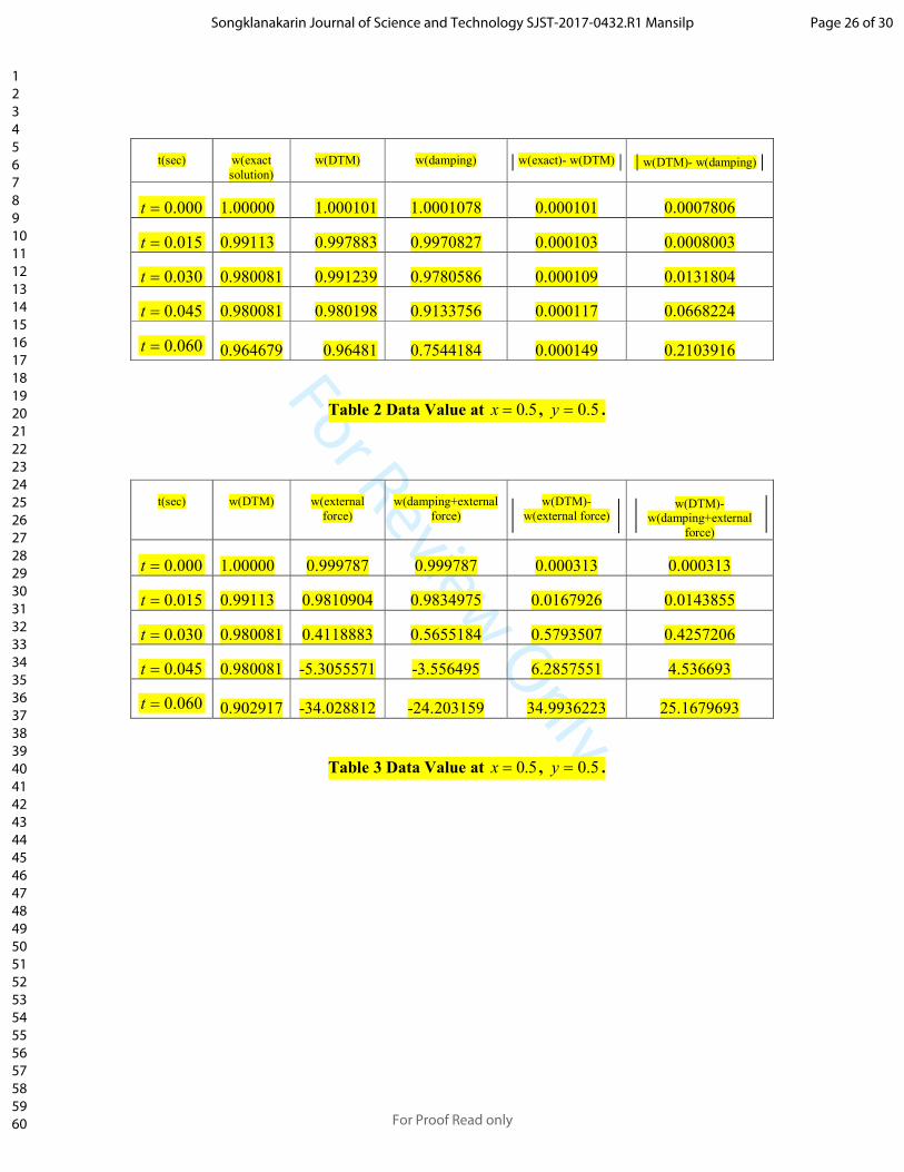
term, as shown by the results in Table (2).
The values for the exact solution, approximate solution with a damping term and error
for the vibration of membrane are shown in Tables 2 below.
Table 2 Data Value at 0.5x = , 0.5y = .
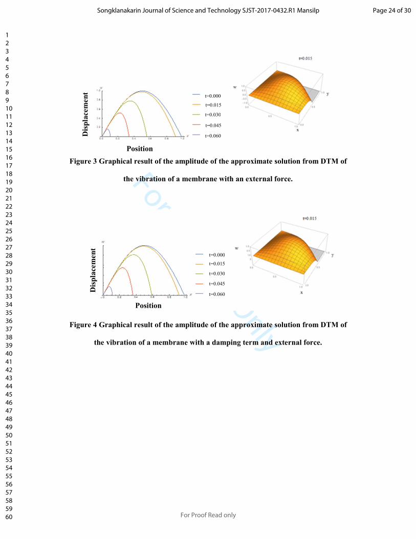
Figure 3 Graphical result of the amplitude of the approximate solution from DTM of
the vibration of a membrane with an external force.
The graphical results of the approximate solution from DTM of the vibration of a
membrane with the external force (Example 4.3) are shown in Fig.3. We found that the
amplitude of vibration is less than that of the vibrating membrane without the external force,
as shown by the results in Table (3).
Figure 4 Graphical result of the amplitude of the approximate solution from DTM of
the vibration of a membrane with a damping term and external force.
The graphical results of the approximate solution from DTM of the vibration a
membrane with a damping term and external force (Example 4.4) are shown in Fig.4. We
found that the amplitude of vibration is less than that of the vibrating membrane without a
damping term and external force as shown by the results in Table (3).
Page 18 of 30
For Proof Read only
Songklanakarin Journal of Science and Technology SJST-2017-0432.R1 Mansilp
123456789101112131415161718192021222324252627282930313233343536373839404142434445464748495051525354555657585960

For Review Only
The values of the approximate solution for the vibration of a membrane with the
external force, with the external force and a damping term, and error for the vibration of a
membrane are shown in Table 3 below.
Table 3 Data Value at 0.5x = , 0.5y = .
6. Conclusions
We found that the analytical solutions and approximate solutions are very similar in
case of the problem with no damping and external force. In the case of the problem with a
damping term and external, the analytical solutions are not solvable. Therefore the DTM is
used to find the approximate solutions. The obtained results show that the addition of a
damping term, and addition of external force in the equation of motion of the membrane, can
cause the amplitude of motion for the vibration of a membrane to decrease.
Acknowledgments
This research is supported by Rajamangala University of Technology Tawan-ok
:Chantaburi Campus, Thailand.
References
Arikoglu, A., & Ozkol, I. (2006). Solution of differential-difference equations by using
differential transform method. Applied Mathematics and computation, 181, 153-162.
Ayaz, F. (2003). On the two-dimentional differential transform method. Applied
Mathematics and computation, 143, 361-374.
Ayaz, F. (2004). Applications of differential transform method to differential-algebraic
equations. Applied Mathematics and computation, 152, 549-657.
Ayaz, F. (2004). Solutions of the system of differential equations by differential
Page 19 of 30
For Proof Read only
Songklanakarin Journal of Science and Technology SJST-2017-0432.R1 Mansilp
123456789101112131415161718192021222324252627282930313233343536373839404142434445464748495051525354555657585960

For Review Only
transform method. Applied Mathematics and computation, 147, 547-567.
Bagheri, M., & Manafianheris, J. (2012). Differential Transform Method for Solving
The Linear and Nonlinear Westervelt Equation. Journal of Mathematical, 3, 81-91.
Biazar, J., & Eslami, M. (2010). Analytic solution for telegraph equation by differential
transform method. Physics letter A, 374, 2904-2906.
Biazar, J., Eslami, M., & Islam, M. R. (2012). Differential transform method for special
systems of integral equations. Journal of King Saud University-Science, 24, 211-
214.
Bildik, N., Konuralp, A., Bek, F. O., & Kucukarslan, S. (2006). Solution of different
type of the partial differential equation by differential transform method and
adomain’s decomposition method. Appliedmathematics and computation, 172, 551-
567.
Catal, S. (2008), Solution of free vibration equations of beam on elastic soil by using
differential transform method. Applied mathematical modeling, 32, 1744-1757.
Chen, C., & Ho, S. (1999). Solving partial differential equations by two- dimentional
differential transform method. Applied Mathematics and computation, 106, 171-
179.
Choi, J., Kumar, D., Singh, J., & Swroop, R. (2016). Analytical techniques for system of time
fractional nonlinear differential equations. Journal of the Korean Mathematical
Society, 54, 1209-1229. doi:10.4134/JKMS.j160423
Hatami, M., Ganji, D., & Sheikholeslami, M. (2017). Differential Transformation
Method for Mechanical engineering problems. Academic Press is an imprint of
Elsevier, United Kingdom.
Jafari, H., Sadeghi, S., & Biswas, A. (2012). The differential transform method for
Page 20 of 30
For Proof Read only
Songklanakarin Journal of Science and Technology SJST-2017-0432.R1 Mansilp
123456789101112131415161718192021222324252627282930313233343536373839404142434445464748495051525354555657585960

For Review Only
solving multidimensional partial differential equations. Indian Journal of Science
and Technology, 5(2).
Kangalgil, F., & Ayaz, F. (2009), Solitary wave solutions for the KdV and mKdV
equations by differential transform method. Chaos, Solitons & Fractals, 41, 464-
472.
Kumar, D., Singh, J., & Baleanu, D. (2017). A New Numerical Algorithm for Fractional
Fitzhugh-Nagumo Equation Arising in Transmission of Nerve Impulses. Nonlinear
Dynamics, doi:10.1007/s11071-017-3870-x
Mirzaee, F., & Yari, M. K. (2015). A novel computing three-dimension differential
transform method for solving fuzzy partial differential equations. Aim Shams
Engineering Journal, 7(2), 695-708.
Ojwando, C. A. (2016). Application of Partial Differential Equations to Drum Head
Vibration, Signal Transmission, and Chemical Communication in Insects, American
Journal of Applied Mathematics, 4, 169-174. doi:10.11648.j.ajam.20160404.11.html
Othman, I. A., & Mahdy, A. M. S. (2010). Differential Transformation method and
variation iteration method for cauchy reaction-diffusion problems. The Journal
Mathematics and Computer science, 2, 61-75.
Prakash, J., Kothandapani, M., & Bharathi, V. (2016). Numerical approximations of
nonlinear fractional differential-difference equations by using Modified He-Laplace
method, Alexandria Engineering Journal, 55, 645-651.
doi:10.1016/j.aej.2015.12.006
Rao, S. (2004). Mechanical Vibrations. University of Miami, Pearson Education,
Inc.publishing as Prentice Hall, NJ 07458.
Saravanan, A., & Magesh, N. (2013). A comparison between the reduced differential
transform method and the Adomain decomposition method for the Newell-
Page 21 of 30
For Proof Read only
Songklanakarin Journal of Science and Technology SJST-2017-0432.R1 Mansilp
123456789101112131415161718192021222324252627282930313233343536373839404142434445464748495051525354555657585960

For Review Only
Whitehead-Segel equation. Journal of the Egyptian mathematical society, 21,
259-265.
Singh, J., Kumar, D., Qurashi, M. A., & Baleanu, D. (2017). A Novel Numerical Approach
for a Nonlinear Fractional Dynamical Model of Interpersonal and Romantic
Relationships. Entropy, 19(7), 375. doi:10.3390/e19070375
Singh, J., Rashidi, M., Sushila, M., & Kumar, D. (2017). A hybrid computational approach
for Jeffery-Hamel flow in non-parallel walls, Neural Computing and Applications,
doi:10.1007/s00521-017-3198-y
Tabaei, K., Celik, E., & Tabaei, R. (2012). The differential transform method for solving
heat-like and wave-like equations with variable coefficients. Turkish journal of
Physics, 36, 87-98. doi:10.3906/fiz-1102-6
Yang, X., Liu, Y., & Bai, S. (2006). A numerical solution of second-order linear partial
differential equations by differential transform. Applied Mathematics and
computation, 173, 792-802.
Zedan, A., & AliAlghamdi, M. (2012). Solution of (3+1)-Dimensional Nonlinear Cubic
Schrodinger Equation by Differential Transform Method. Mathematical Problems in
Engineering, doi:1155/2012/531823
Page 22 of 30
For Proof Read only
Songklanakarin Journal of Science and Technology SJST-2017-0432.R1 Mansilp
123456789101112131415161718192021222324252627282930313233343536373839404142434445464748495051525354555657585960
For Review Only
Figure 1 Graphical comparison between the amplitude of the analytical solution and the
approximate solution from DTM of the vibration of a membrane.
Figure 2 Graphical result of the amplitude of the approximate solution from DTM of
the vibration of a membrane with a damping term.
0.2 0.4 0.6 0.8 1.0X
0.2
0.4
0.6
0.8
1.0
W t DTM 0.000
t DTM 0.015
t DTM 0.030
t DTM 0.045
t DTM 0.060
t Analytical 0.000
t Analytical 0.015
t Analytical 0.030
t Analytical 0.045
t Analytical 0.060
Displacement
Position
Displacement
Position
t=0.060
t=0.045
t=0.030
t=0.015
t=0.000
Page 23 of 30
For Proof Read only
Songklanakarin Journal of Science and Technology SJST-2017-0432.R1 Mansilp
123456789101112131415161718192021222324252627282930313233343536373839404142434445464748495051525354555657585960
For Review Only
Figure 3 Graphical result of the amplitude of the approximate solution from DTM of
the vibration of a membrane with an external force.
Figure 4 Graphical result of the amplitude of the approximate solution from DTM of
the vibration of a membrane with a damping term and external force.
Displacement
Position
t=0.060
t=0.045
t=0.000
t=0.015
t=0.030
Displacement
Position
t=0.060
t=0.045
t=0.015
t=0.000
t=0.060
t=0.030
Page 24 of 30
For Proof Read only
Songklanakarin Journal of Science and Technology SJST-2017-0432.R1 Mansilp
123456789101112131415161718192021222324252627282930313233343536373839404142434445464748495051525354555657585960

For Review Only
The fundamental operations of three-dimensional differential transform method
Original function Transformed form
2
2
( , , )3.1 ( , , ) ( , , )
w x y tv x y t a x y t
x
∂=
∂
0 0 0
( , , ) ( 2)( 1)
( , , ) ( 2, , ).
k h m
i j r
V k h m k i k i
A i j r W k i h j m r
= = =
= − + − +
− + − −
∑∑∑
2
2
( , , )3.2 ( , , ) ( , , )
w x y tv x y t b x y t
y
∂=
∂
0 0 0
( , , ) ( 2)( 1)
( , , ) ( , 2, ).
k h m
i j r
V k h m h i h i
B i j r U k i h j m r
= = =
= − + − +
− − + −
∑∑∑
2
2
( , , )3.3 ( , , ) ( , , )
w x y tv x y t c x y t
t
∂=
∂
0 0 0
( , , ) ( 2)( 1)
( , , ) ( , , , 2).
k h m
i j r
V k h m m i m i
C i j r W k i h j m r
= = =
= − + − +
− − − +
∑∑∑
( , , )3.4 ( , , ) ( , , )
w x y tv x y t d x y t
t
∂=
∂ 0 0 0
( , , ) ( 1) ( , , )
( , , ) ( , 1, ).
k h m
i j r
V k h m h i D i j r
D i j r W k i h j m r
= = =
= − +
− − + −
∑∑∑
3.5 ( , , )n l s
v x y t x y t=
( , , ) ( , , ) (( ) ( ) ( ),
1 , 1 , 1 ,( ) ( ) ( )
0 , 0 , 0 ,
V k h m k n h l m s k n h l m s where
k n h l m sk n h l m p
k n h l m s
δ δ δ δ
δ δ δ
= − − − = − − −
= = = − = − = − =
≠ ≠ ≠
3.6 ( , , ) ( , , ) ( , , )n
v x y t p x y t w x y t=
1 1 1 3 13 32 2 2
1 2 1 2 1 2 2 1 2 1 2 10 0 0 0 0 0 0 0 0 0 0 0
1 1 1 1 2 2 1 2 1 2 1
1 1 2 1 2 1 2 1 1
( , , ) ...
( , , ) ( , , )...
( , , ) ( , ,
n n n
n n n n n n
mk h m k h mk hk h m
k k h h m m k k h h m m
n n n n n n n n n n
V k h m
W k h m W k k h h m m
W k k h h m m W k k h h
− − −
− − − − − −= = = = = = = = = = = =
− − − − − − − − −
=
− − −
− − − − −
∑ ∑ ∑ ∑ ∑ ∑ ∑∑∑∑∑∑
1).nm m−−
33.7 ( , , ) ( , , ) ( , , )v x y t q x y t w x y t=
2 2 2
2 1 2 1 2 1
1 1 1 1
0 0 0 0 0 0
2 2 1 2 1 2 1 3 2 2 2
( , , )( , ,
( , , ) ( , ).
)
,
k h mk h m
k k h h m m
W k h m
W k k h h m m
V k h m
W k k h h m m
= = = = = =
− − − − −
=
−
∑∑∑∑∑∑
Table 1 The fundamental operations of DTM
Page 25 of 30
For Proof Read only
Songklanakarin Journal of Science and Technology SJST-2017-0432.R1 Mansilp
123456789101112131415161718192021222324252627282930313233343536373839404142434445464748495051525354555657585960
For Review Only
t(sec) w(exact
solution)
w(DTM) w(damping) w(exact)- w(DTM)
w(DTM)- w(damping)
0.000t = 1.00000 1.000101 1.0001078 0.000101 0.0007806
0.015t = 0.99113 0.997883 0.9970827 0.000103 0.0008003
0.030t = 0.980081 0.991239 0.9780586 0.000109 0.0131804
0.045t = 0.980081 0.980198 0.9133756 0.000117 0.0668224
0.060t =
0.964679 0.96481 0.7544184
0.000149 0.2103916
Table 2 Data Value at 0.5x = , 0.5y = .
t(sec) w(DTM) w(external
force)
w(damping+external
force)
w(DTM)-
w(external force)
w(DTM)-
w(damping+external
force)
0.000t = 1.00000 0.999787 0.999787 0.000313 0.000313
0.015t = 0.99113 0.9810904 0.9834975 0.0167926 0.0143855
0.030t = 0.980081 0.4118883 0.5655184 0.5793507 0.4257206
0.045t = 0.980081 -5.3055571 -3.556495 6.2857551 4.536693
0.060t =
0.902917 -34.028812 -24.203159 34.9936223 25.1679693
Table 3 Data Value at 0.5x = , 0.5y = .
Page 26 of 30
For Proof Read only
Songklanakarin Journal of Science and Technology SJST-2017-0432.R1 Mansilp
123456789101112131415161718192021222324252627282930313233343536373839404142434445464748495051525354555657585960

For Review Only
The calculation of the examples 4.2.
2 2 2
2 2 2,
w w w w
tt x y
∂ ∂ ∂ ∂= + −
∂∂ ∂ ∂ (1)
The initial conditions are:
( , ,0) sin sin , 0 , 0 ,
( , ,0) 0, 0 , 0 ,
x yw x y x a y b
a b
wx y x a y b
t
π π= ≤ ≤ ≤ ≤
∂= ≤ ≤ ≤ ≤
∂
(2)
we assumed that 1a = and 1b = .Therefore, the boundary conditions of the equation of
motion of a membrane are definded thus:
( ,0, ) 0, 0 1,
(0, , ) 0, 0 1,
( ,1, ) 0, 0 1,
(1, , ) 0, 0 1, .
w x t x
w y t y
w x t x
w y t y t
= ≤ ≤
= ≤ ≤
= ≤ ≤
= ≤ ≤ ∈ �
(3)
An analytical solution
The following is the derivation of the analytical solution with damping term.
Considering the initial conditions ( , ,0) sin sinw x y x yπ π= and ( , ,0) 0,w
x yt
∂=
∂ the boundary
conditions are shown in (2).The general solution can be derived by the separation of variables
technique:
( , , ) ( ) ( ) ( ),w x y t X x Y y T t= (4)
Subject to the eigenvalue, 2 2,ω α− and
2β , can be written (1)
( ) ( ) ( ) ( ),
( ) ( ) ( ) ( )
T t X x Y y T t
T t X x Y y T t
′′ ′′ ′′ ′= + −
2( ) ( ),
( ) ( )
X x Y y T T
X x Y y T Tω
′′ ′′ ′′ ′+ = + = −
Page 27 of 30
For Proof Read only
Songklanakarin Journal of Science and Technology SJST-2017-0432.R1 Mansilp
123456789101112131415161718192021222324252627282930313233343536373839404142434445464748495051525354555657585960

For Review Only
and
2 2( ) ( ),
( ) ( )
X x Y y
X x Y yω α
′′ ′′− = + =
2( ),
( )
X x
X xα
′′− =
then 2( ) ( ) 0,X x X xα′′ + =
2 2( )( ),
( )
Y y
Y yω α
′′= − −
assumed 2 2 2 ,ω α β− =
then 2( ) ( ) 0,Y y Y yβ′′ + =
then 2( ) ( ) 0,X x X xα′′ + = (5)
2( ) ( ) 0Y y Y yβ′′ + = , (6)
2( ) ( ) ( ) 0.T t T t T tω′′ ′+ + = (7)
We obtain a solution of (5) as 1 2( ) cos sin ,X x C x C xα α= + where 1C and 2C are arbitrary
constants. Subject to the boundary conditions (0) 0X = , we have 1 0.C = Then
2( ) sinX x C xα= full step the boundary condition (1) 0.X = Let 2 0C ≠ give ;m m Iα π= ∈ ,
we have that
( ) sinm mX x C m xπ= . (8)
We obtain a solution of (6) as 3 4( ) cos sinY y C x C yβ β= + .According to boundary
conditions (0) 0Y = , we have 3 0.C = Then the boundary conditions ( ) 0Y y = .
Letting 4 0C ≠ gives ;n n Iβ π= ∈ , then we see that:
( ) sin .n nY y C n yπ= (9)
From
Page 28 of 30
For Proof Read only
Songklanakarin Journal of Science and Technology SJST-2017-0432.R1 Mansilp
123456789101112131415161718192021222324252627282930313233343536373839404142434445464748495051525354555657585960

For Review Only
2 2 2
2 2
,
.m n
ω β α
ω π
= +
= +
2( ) ( ) ( ) 0.T t T t T tω′′ ′+ + =
2 2 0r r ω+ + =
21 1 4,
2 2r
ω−= − ± (10)
We obtain a solution of (7) as
2 2
2, , ,
1 4 1 4( ) ( cos sin )
2 2
t
m n m n m nT t e A t B t
ω ω− − −= + . (11)
According to (8), (9) and (11) can be written
2
2
2
2
( , , ) ( ) ( ) ( ),
1 4sin sin cos
2
1 4sin sin sin ,
2
mn
t
mn m n
t
mn m n
W x y t X x Y y T t
A C C m x n y t e
B C C m x n y t e
ωπ π
ωπ π
−
−
=
−= ⋅
−+ ⋅
(12)
where mn mn m nF A C C= , mn mn m nH B C C= and for all 1,2,3,...mn =
By using the superposition principle (12) become
1 1
2
2
1 1
2
2
( , , ) ( , , ),
1 4sin sin coscos ,
2
1 4sin sin sin cos .
2
mn
m n
t
mn
m n
t
mn
w x y t w x y t
F m x n y t e
H m x n y t e
ωπ π
ωπ π
∞ ∞
= =
−∞ ∞
= =
−
=
−= ⋅
−+ ⋅
∑∑
∑∑ (13)
According to the initial condition ( , ,0) sin sinw x y x yπ π= and ( , ,0) 0.w
x yt
∂=
∂ By using
Fourier series, we have
Page 29 of 30
For Proof Read only
Songklanakarin Journal of Science and Technology SJST-2017-0432.R1 Mansilp
123456789101112131415161718192021222324252627282930313233343536373839404142434445464748495051525354555657585960

For Review Only
2
1 ; 1 1, 2
1.
1 8
mn
mn
F m and n
H
ω π
π
= = = =
=−
Substituting 1mnF = and2
1
1 8mn
Hπ
=−
in (13), we obtain the analytical solution:
2 2
2
2
1 8 1 1 8( , , ) (cos sin )(sin sin )
2 21 8
t
w x y t e t t x yπ π
π ππ
− − −= +
− (14)
Since 2ω π= when substituting to (11), we obtain that 21 4ω− is complex number.
Therefore
( )T t can not be solved.
Page 30 of 30
For Proof Read only
Songklanakarin Journal of Science and Technology SJST-2017-0432.R1 Mansilp
123456789101112131415161718192021222324252627282930313233343536373839404142434445464748495051525354555657585960


