
United Arab Emirates UniversityScholarworks@UAEU
Theses Electronic Theses and Dissertations
2008
Flow in Porous Media and Environmental ImpactNoujoud M Jawhar
Follow this and additional works at: https://scholarworks.uaeu.ac.ae/all_theses
Part of the Environmental Sciences Commons
This Thesis is brought to you for free and open access by the Electronic Theses and Dissertations at Scholarworks@UAEU. It has been accepted forinclusion in Theses by an authorized administrator of Scholarworks@UAEU. For more information, please contact [email protected].
Recommended CitationJawhar, Noujoud M, "Flow in Porous Media and Environmental Impact" (2008). Theses. 419.https://scholarworks.uaeu.ac.ae/all_theses/419
United Arab Emirate University
Dean hip of Graduate Studies M.Sc. Program in Environmental Sciences
FLOW IN POROUS MEDIA AND ENVIRONMENT AL IMPACT
By
Noujoud M. Jawhar
A thesis
Submitted to
The United Arab Emirates University
In partial fulfillment of the requirements
for the degree of M.Sc. in Environmental Sciences
2008

United Arab Emirates Uni versity Deanship of Graduate Studies
M.Sc . Program in Environmental Sciences
FLOW IN POROUS MEDIA AND EVIRONMENTAL
IM PA C T
By
Noujoud M. Jawhar
A thesis Submitted to
United Arab Emirates University In partial fulfi l lment of the requirements
For the degree of M .Sc. in Environmental Sciences
SUP ERVISED BY
Dr. F. Allan Dr. M. Anwar Dr. M. Syam
Professor Professor Professor
Department of Department of Head Department of Mathematics Mathematics Mathematical Sciences
Faculty of Science Acting Dean, College of Faculty of Science Science
UAE University UAE University UAE University
11

The The i of Noujoud Mohamed Jawhar for the Degree of Ma ter of ci nc in Environmental is approved.
4�···· ............... .
Examining Committee Member, Dr. Fathi M. Allan
Examining Committee Member, Dr. Ali Mohammed Sayfy
Examining Committee Member, Dr. Saud Khashan
it . . . . . . . . . . . . . . . . . . . . . . . . . . . . . . . . . . . . . . . . . . . . . . . . . . . . . .
s istant Chief Academic Officer for Graduate Studies, Prof. Ben Bennani
United Arab Emirates University
200812009
A CKNOWLEDGMENT
FIrst and foremost, I want to thank all members of the United Arab Emirates
niversity for providing an excel lent and inspiring working atmosphere . In particular,
the director of the environmental sciences graduate program, Dr. Tarek Youssef, who
has created an optimum infrastructure, so that a lack of resources is unimaginable . His
managerial ski l l s and uncompromising quest for excellence shape all his students
signi ficantly during their time at the institute. I would also l ike to thank the faculty
and staff at the United Arab Emirates University for the help and support throughout
the course of my studies, in partic ular, Dr. Abdul Majeed A l khajah, Dr. Mohamad el
Deeb, and Dr. Waleed Hamza. A special thanks to Dr. Muhammad Hajj i for his
enormous support and help with Mathematica while developing the mathematical
models .
Thi s work would not have been completed without help and support of many
individuals. I would l ike in particular to thank my advisor Dr. Fathi Al lan for his great
insight, help, and very useful advice and guidance throughout the course of my
research at UAEU. I truly learned a lot from him from both technical as well as
professional perspectives. I have a lways appreciated and admired h is motivation and
dri ve for excellence.
I also would l ike to thank the other members of my committee, Dr.
Mohammad N. Anwar and Dr. Muhamad Syam for their guidance and assistance
which was very valuable and indispensable in the process of completing this research .
I thank them for taking from their valuable t ime to direct, and support this work.
111

Finally. I am very grateful for the support of my parents, my sisters. and my
brothers, and my husband Imad for his enduring patience, understanding, and love,
and my precIOus chi ldren Alaa. Hassan, and Hanan who were my great inspiration .
They pro ided me wi th indispensable support that was essential during the course of
my study, and for the completion of this work .
i v

ABSTRACT
Recently, a great deal of interest has been focused on the investigation of
transport phenomenon in di sordered systems . In particular, fluid flow through porous
media has attracted m uch attention due to its importance in several technological
processes such as fi l tration. catalysis, chromatography spread of hazardous wastes,
petroleum exploration, and recovery. Furthermore, flow through porous media is an
important environmental problem that has environmental impl ications in several areas
such as the study of poll ution, fate of contaminants, contaminations issues re lated to
agriculture, c iv i l constructions, coastal management, and many more .
In this thesis, the f luid flow through mult i- layers porous media is investigated.
A mathematical model for the flow velocit ies is set to describe the flow through these
different layers, together wi th initial and boundary conditions. More attention is made
to the veloci ty profiles at the interface. The model is then sol ved with two different
methods the shooting method and the finite difference method. We consider a finite
width three porous layer problem, where the layers have different permeabi l i ty values
which introduce a discontinui ty in the penneabi l i ty at the interface region . At the
interface the continuity of the veloci ty and shear stress are imposed. A comparison
between the nonl inear shooting method and the finite difference approach is then
made and it shows that the shooting method is more accurate and more efficient.
v

TABLE OF CONTENTS
Section Title Page
Nu mber
Supervi or's Page ii
Acknowledgements i i i
Ab tract (in English) v
Table of Contents vi
Li t of Tables ix
List of Figures x
1.0 INTRODUCTION 1.1 Porous Medi um 1
1 .2 Porosity 4
1 .2 . 1 Factors Affecting Porosity 5
A. Uniformity of grain size 5
B. Degree of cementation 5
C. Amount of compaction 5
1 .2 .2 Classification of Porosity 6
1.3 Darcy's Law 7
1.4 Permeability 1 0
1 .4. 1 Classification of Permeabi l i ty 14
1 .5 Soi l Structure 1 5
1.6 Water Movement 1 6
1 .6 . 1 Water Movement Through Soi l 18
VI
1 .6 .2 How Soil Texture A ffects Water Movement 1 9
l .6 .3 Infiltrat ion 20
1.7 Saturated Vs. Unsaturated Flow 2 1
1 .7. 1 Unsaturated Water Flow 2 1
l .7 .2 Saturated Water Flow 22
2.0 OBJECTIVES 23
3.0 MA TERIALS AND METH ODS 25
4.0 MA THEMAT I C A L MOD E L ING OF FLllD FLOW IN
POROUS MEDIA 4.1 Simple Mathematical Model 27
5.0 NUMERICAL METHODS
5.0 More Complicated Mathematical Model
5.1 Finite Difference Approach 34
5.2 Non Linear Shooting Method 40
6.0 FLUID FLOW T HROU G H MUL T ILAYER OF 42
FIN I TE DEPTH
7.0 RESULTS 46
Vll

8.0 ENVIRONMENTAL IMPA C T 5 5
9.0 REFERENCES 58
ABSTRACT I N A RABIC
TITLE PAGE IN A RABI C
vi i i

LIST OF TABLES
Table I Values of Hydraulic Conductivity 1 3
Table I I Values of Penneabi l i ty 1 3
Table III Values of Porosity and Penneabili ty 1 4
Table IV Case 1 : shooting method Vs . Fini te difference 49
Table V Case 2: shooting method Vs . Fin i te difference 49
Table VI Case 3: shooting method Vs. Fin i te difference 50
ix
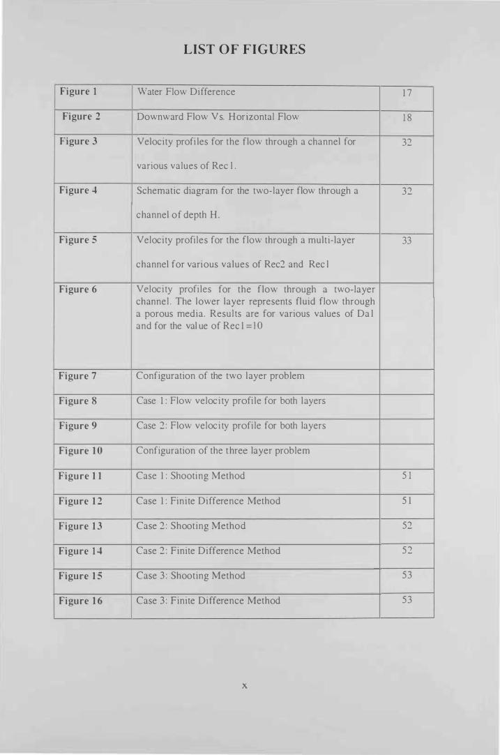
LIST O F FIGURES
Figure 1 Water Flow Difference 1 7
Figure 2 Downward Flow V s. Horizontal Flow 1 8
Figure 3 Velocity profi les for the flow through a channel for 32
various values of Ree l .
Figure 4 Schematic diagram for the two-layer flow through a 32
channel of depth H .
Figure 5 Veloci ty profi les for the flow through a multi- layer 33
channel for various values of Rec2 and Rec l
Figure 6 Veloc i ty profi les for the flow through a two-layer channel . The lower layer represents fluid flow through a porous media. Resul ts are for various values of Da l and for the val ue of Rec 1 = 1 0
Figure 7 Configuration of the two layer problem
Figure 8 Case I: Flow veloc i ty profi le for both layers
Figure 9 Case 2 : Flow veloc i ty profi le for both layers
Figure 1 0 Configuration of the three layer problem
Figure 1 1 Case 1 : Shooting Method 5 1
Figure 1 2 Case 1 : Fini te Difference Method 5 1
Figure 1 3 Case 2 : Shooting Method 52
Figure 1 4 Case 2 : Finite Difference Method 52
Figure 1 5 Case 3 : Shooting Method 53
Figure 1 6 Case 3 : Finite Difference Method 53
x

1. 0 I TRaDUCTION
1.1 Porou Medium
A porous medium is a material that consists of a solid matrix with an
interconnected void. The interconnec tedness of the pores a l lows the flow of one or
more fl uids though the material. In the simplest situation which is a single phase flow,
the void is saturated by a single fluid . In two phase fl ow, a liquid and a gas share the
void pace. Fluid flow in a porous medium resembles that of a pouring a cup of water
for example over soil and letting the water flow into the soil due to the gravi tational
forces [ 1 ] .
A porous material or structure must pass at least one of the fol lowing two tests
in order to be qualified as a porous medium. The first test, it must contain spaces,
cal led pores or voids, free of solids imbedded in the solid or semisolid matrix . The
pores usually contain some fl uid, such as water, oil, or a mixture of different fluids.
The second test is that i t must be permeable to a variety of fluids . That is fl uids should
be able to penetrate through one face of the material and emerge on the other side. To
disti nguish between a porous sol id and jus t any sol id is a straight-forward process
since the infi l tration of viscous flow is a predetermined condi tion for the material to
qual ify as a porous medium.
Porous materials are encountered l i teral ly everywhere in everyday l ife, in
technology, and in nature . Many natural substances such as rocks, and biological
tissues such as lungs and bones, and man made materials such as cements, foams and
ceramics can be considered as porous media. More examples of porous material
inc lude soil which is capable of performing i ts function of sustaining plant l ife only

becau e it can hold water in i ts pore spaces. Bui lding materials such as bricks,
concrete, l imestone, and sand tone are examples of porous materials and they are
considered to be better thermal insulators because of their porous nature [2 ] .
The concept of porous media i s used in many areas of applied science and
engineering. It is used in mechanics such as geo-mechanics, soi l and rock mechanics,
in engineering such as petroleum and construction engineering, in geosciences such as
hydrogeology and geophysics, in biology and biophysics, in material sciences, and
many more fie lds of science. However, the most important areas of technology that
depend significant ly on the properties of porous media are hydrology, which relates to
water movement in earth and sand structures , petroleum engineering which is mainly
concerned with petroleum, and natural gas production, exploration well dri l l ing, and
logging [ 1 ]. Additionally, the flow of blood and other body fluids and electro-
osmosis are few examples where porous m edia plays a cri tical role in medicine and
biological engineering. Fluid flow through porous media has emerged as a separate
field of study because it i s a subject of most common interest [3].
The porosi ty cp and the permeabili ty k are two important quanti ties that
describe the properties of a porous medi um. The porosity of a porous medi um is
defined as :
pore volume matrix volume
(1 .0 )
where the pore volume denotes the total volume of the pore space in the matrix and
the matrix volume is the total vol ume of the matrix including the pore space. Thus,
porosity is greater than or equal zero and less than or equal 1 . Porosity equals to zero
2

when the pore volume equals to zero, i . e . there is no flow. Porosity equals to 1 when
the pore olume is the same as the matrix volume [4] .
The permeabi l i ty k describes the abi l i ty of the fl uid to flow through the porous
medium. It is often cal led the absolute permeabi l i ty, and it is a quantity that depends
only on the geometry of the medium. There has been much effort to establ ish relations
between the permeabi l i ty and the porosity. However, a general formula seems to be
impossible to find, and the permeabi l i ty is found to be proportional to rpm, where m is
in the range of 3 to 6 depending on the geometry of the medium [3 ,4],
The fl uid flowing in the pore space is characterized by the dynamical vi scosi ty
Jl. The viscosi ty indicates the resistance i n the fluid due to i ts deformations. At the
microscopic level there are friction forces in the fluid caused by the in terchange of
momentum in col l isions between the molecules. Thus, the viscosity of the fluid is set
by the strength of the friction forces [3] .
Fluid flow through a porous medium is often given by the Darcy equation .
Consider a porous medium of absolute permeabi l i ty k in a homogeneous gravi tation
fie ld where one fl uid of vi scosity Jl is injected through the medium by applying a
pressure gradient \1 P across the matrix . Then the flow rate U of the fl uid through the
medium is given by Darcy's equation :
-7 k �
U = - - (\1P- pg) ,u
(1 . 1 )
Where g denotes the acceleration due to the gravi tational forces and p is the
densi ty of the fI uid [4] .
3

1.2 Porosity
From a hydrologic point of VIew, the fundamental interests in a porous
medium are i ts abi li ty to hold and transmit water. Porosi ty is the most important term
among many other terms that relate to the water holding potential of a medium. The
porosity <p of a porous medium is defined as the fraction of the total volume of the
medium that is occupied by void space such as in equation ( 1 .0) .
In defining <p in this way a l l the void space is assumed to be connected. If
some of the pore space in a medium are disconnected from the remainder, then
effective porosity is introduced which is defined as the ratio of connected voi d to total
olume. Depending on the type of the porous medium, the porosi ty may vary from
near zero to almost unity . For example certain types of volcanic rocks have very low
porosities, while fibrous filters and insulators are highly porous substances [5]. There
are many types of void space, but it is important to distinguish between two kinds of
pore space. The first one forms a continuous phase within the porous medi um cal led
interconnected or effecti ve pore space . The other one consists of isolated or non
interconnected pores dispersed over the medium. Moreover, pore space has a direct
effect upon productive value of soi ls because of its influence upon water holding
capac i ty and upon the movement of air, water, and roots through the soi l . For
example, when the pore space of a productive soi l is reduced 1 0 percent, movement of
air, water, and roots is greatly restric ted and growth is very seriously impeded [1].
1 .2. 1 Factors Affecting Porosity
There are many factors that affect porosity. and there has been a lot of effort
done to determine approximate l imits of porosities values . The factors governing the
magnitude of porosity are the fol lowing.
4

A. Uniformity of grain size : unifonnity or sorting is the gradation of grains.
If small particles of si l t or c lay are mixed wIth larger sand grains, the effective
porosi ty wil l be considerably reduced. Sorting depends on at least four major
factors which are size range of the material , type of deposition current
characteristics, and the duration of the sedimentary process [ 5] .
B. Degree of cementation: The highly cemented sandstones have low
porosi ties, whereas the soft unconsol idated rocks have high porosities. The
cementation process is very essenti al because fi l l ing void space with mineral
material wil l reduce porosity.
C. Amount of compaction: Duri ng and after deposition, compaction tends
to close voids and squeeze fluid out to bring the mineral particles closer
together especial ly the finer grained sedimentary rocks. Generally porosi ty is
lower in deeper, older rocks, but exceptions to this basic trend are common
[ 5 ] .
5

1 .2.2 Cia sification of porosity
Additional tenns should be introduced regarding tenninology with respect to
the porosity namely the primary and the secondary fonns. The primary porosity refers
to the original porosity of the medium upon deposition . Secondary porosity refers to
that portion of the total porosity resulti ng from processes such as dissol ution. For
example, l imestone has a very low primary porosity upon deposition . If raised above
sea leveL di ssolution processes can lead to the fonnation of caves with very large
secondary porosity. A similar interpretation applies to the distinction between solid
and fractured rock. The rock matrix has very low porosity. The presence of fractures
increases the secondary porosity over the primary porosity. The secondary porosity of
a medi um is not always greater than its primary porosity, for example, a sand deposit
that may become cemented over time to form sandstone. The chemical ly precipitated
cementing agents occupy part of the pore space, therefore reducing the overall
porosity [ 1 , 4] .
During sedimentation some of the pore spaces initia l ly developed became
isolated from the other pore spaces by various processes such as cementation and
compaction. Thus. many of the pores wil l be interconnected, whereas others wi l l be
completely i solated. This leads to two disti nct categories of porosity, namely total or
absolute and effective. Absolute porosity i s the ratio of the total void space in the
sample to the bu lk volume of that sample regardless of whether or not those void
spaces are interconnected. A rock may have considerable absolute porosity and yet
have no fluid conducti vity for lack of pore interconnection . Examples of this are lava
and pumice stone .
Effective porosity is the ratio of the interconnected pore volume to the bulk
volume. Thi s porosity is an indication of the abil ity of a rock to conduct fluids, but it
6

should not be used as a measure of the flu id conductivity of a rock. It is affected by a
number of factors inc luding the type, conten t and hydration of the c lays present in the
rock, the heterogeneity of grain sizes, the packing and cementation of the grains, and
any weathering and leaching that may have affected the rock. Experimental
techniques for measuring porosi ty must take these facts into consideration [ 1 3, 5 ] .
For natural media, <t> does not normal ly exceed 0 .6 . For beds of solid spheres
of uniform diameter, <t> varies between 0. 2545 and 0.4764. For man made materials
such as metal l ic foams <t> can approach the val ue l . Table I I I i l l ustrates the different
values of porosity and other properties of common porous materials [4] .
1.3 DA RCY'S LAW
The science of groundwater flow originates from about 1 856, in which year
the c i ty engineer of Dijon, Hemy Darcy, published the results of the investigations
that he had carried out for the design of a water supply system based on subsurface
water carried to the val ley in which Dijon i s located, by permeable layers of soi l , and
supplied by rainfal l on the surroundings. Since that time the basic law of groundwater
movement carries h is name, but the presentation has been developed, and the law has
been generalized in several ways [6 ] . Henry Darcy's investigations revealed
proportional i ty between flow rate and the applied pressure di fference. In modern
notation this is expressed by equation ( l . 1 ) , where 'V P is the pressure gradient in the
flow direction, and J.l is the viscosity of the fluid. The coefficient k is the permeabil i ty,
and it is independent of the nature of the fl uid but i t depends on the geometry of the
medium, U is the flow rate, g denotes the acceleration due to the gravi tational forces,
and p is the density of the fluid.
7

It is useful [0 consider as a point of reference, the hydrostatics in a porous
medium, the pores of which are completely filled with a fluid of density p . If the
pressure in the fluid is denoted by p, the principles of hydrostatics teach that in the
absence of flow the pressure increases with depth, and the local pressure gradient is
equal to pg, where g is the gravity acceleration. Thus, with the positive z-axis
pointing upwards, if there is no flow we have:
ap = 0 , ax
ap = 0 , ay
ap + pg = 0 , a:::
(1 .2 )
(l.3 )
(1.4 )
These equations express equilibrium of the pore fluid. They are independent of
the actual pore geometry, provided that all the pores are interconnected [1].
In the case when the pore fluid moves with respect to the solid matrix a frictional
resistance is generated, due to the viscosity of the fluid and the small dimensions of
the pores. The essence of Darcy's experiments result is that for relatively slow
movements the frictional resistance is proportional to the flow rate. If inertia effects
are disregarded, and if the porous medium is isotropic, that is the geometry of the pore
space is independent of the direction of flow, the equations of equilibrium can be
written as:
ap + jl qx = 0 ax k
8
(l . 5 )
(1.6)

CJp 11 -+-q� = O CJ;: k ' (1.7 )
Where )..l is the viscosity of the fluid, and k indicates the permeability of the
porous medium. The quantities qx, qy, and qz, are the three components of the
specific discharge vector, where specific discharge denotes the discharge through a
certain area of soil, di vided by that area [6] .
Darcy's law is a simple mathematical statement which summarizes several
familiar properties that groundwater flowing in aquifers demonstrates. Such properties
include first if there is no pressure gradient over a distance, no flow occurs. Second
if there is a pressure gradient, flow will occur from high pressure towards low
pressure; the greater the pressure gradient the greater the discharge rate. Third, the
discharge rate of fluid will often be different through different formation materials, or
even through the same material in a different direction, even if the same pressure
gradient exists in both cases [3, 5 6 ] .
9

1.3 PERMEAB I L I TY
It is the term used for the conductivity of the porous medium with respect to
permeation by a fluid. It has limited usefulness because its value in the same porous
ample may vary with the properties of the permeating fluid and the mechanism of
permeation. This quantity is called permeability k, and its value is uniquely
determined by the pore structure. Darcy is the practical unit of permeability [3, 4]. A
porous material has k equals to 1 Darcy if a pressure difference of 1 atmosphere will
produce a flow rate of 1 cm3/sec of a fluid with 1 cP viscosity through a cube having
sides 1 cm of length. Thus:
1 Darcy [�*lep)
sec (1 .8 )
(latm 3) , --*lem em
One Darcy is a relatively high permeability, and the permeability of most
reservoir rock is less than one Darcy.
Measurement of permeability in the case of isotropic media is usually done on
linear, mostly cylindrically shaped, core samples. The experiment would be arranged
in a way to have either horizontal or vertical flow through the sample. Both liquids
and gases have been used to measure penneability. However, liquids sometimes
change the pore structure, thus the permeability changes as well, and that is due to the
rearrangement of some particles, swelling of certain materials in the pores such as
clays, and chemical reactions. In principle, measurement at a single steady flow rate
permits calculation of the permeability from Darcy's law, however there is usually
considerable experimental error when measuring, that is why it is advised to perform
measurements at various low flow rates, plot the low rates versus the pressure drop
1 0

and fit a straight line to the data point. According to Darcy's law, this line must pass
through the origin. However, the scatter of the data points might sometimes cause the
best fitting straight line not to pass through the origin. If the dara points cannot be
fitted with a straight line, the Darcy's law is not applicable and the system needs to be
investigated to find the reasons of the deviation [1, 3, 6].
There are two parameters that describe the permeability, the penneability k,
and the hydraulic conductivity K, related to each other by the following equation:
Where p is the density of the fluid, g is the gravity, and j...l is the fluid's
iscosity. The most fundamental property is the permeability k which only depends
upon the properties of the pore space. Because of the factors 11 and p in this equation
the hydraulic conductivity also depends upon the fluid properties, in particular upon
the viscosity. This means that more effort is required to let a more viscous fluid flow
through a porous medium. It also means that K through the viscosity depends upon
the temperature. In areas with great fluctuations between the temperatures in summer
and winter, seasonal variations in the groundwater discharge may result [5].
One of the most important properties of soils is the velocity of water flow though
the pore spaces caused by a given force. A measure of how easily a fluid, for example
water, can pass through a porous medium for example soils. The permeability of soil
is defined as the velocity of flow caused by a unit hydraulic gradient. It is not
influenced by the hydraulic slope, and this is an important point of difference between
permeability and infiltration. Also the tenn permeability is used for designating flow
through soils in any direction. It is influenced most by the physical properties of the
soil. In saturated field soils penneability varies between wide limits: from less than 1
11

foot per year in compact clay soils, up to several thousand feet per year in gravel
formations. For unsaturated soils, the moisture content is one of the dominant factors
influencing permeability [7, 8, 9].
Furthermore, many physical and chemical characteristics of soils are related to
their texture. Fine grained soils have a much larger surface area than coarse grained
oils. Thus, their mineral structure is different, resulting in a much greater capacity for
sorption of chemicals. On the other hand, well sorted, coarse grained soils have a
much smaller sorption capacity and a much larger permeability, for example,
cemented sediments include sandstone and shale. Depending on the degree of
cementation, sandstone can be very permeable and can serve as an excellent source
for water supply. Shale has very low permeability because shale deposits are hydro
geologically significant when they act as confining beds bounding more permeable
strata. Carbonate rocks such as limestone have relatively high amounts of void space
but have low permeability. Igneous and metamorphic rocks have small amounts of
void space about less than 1 percent of the rock mass. In addition, the few present
pores are small and not interconnected, resulting in permeabilities that may be
regarded as zero for almost all practical problems [5 10, 1 1]. However, all rocks such
as sedimentary, igneous, and metamorphic can be fractured by earth stresses. Tables I
and II illustrate the different values of permeability and hydraulic conductivity of
common porous materials Fractured rock is quite different from unfractured rock and
that is because water may move easily through the fractures giving the rock mass a
higher permeability although not much capability for storing water within the pore
space. In addition, rock that is fractured by earth stresses may develop directional
characteristics to its permeability, having a greater potential for allowing flow in
certain directions.
12

Table I Values of Hydraulic Conductivity
Material Hydraulic cond uctivity K (m/s) Clay 1 0-1 U to 1 0-15 Silt 1 0-lS to 1 0-0 Sand 1O.� to 1 0-) Gravel 1 0-': to 1 0-1
Table I I Values of Permeability
Material Permeability k (m.t) Clay 1 0-1/ to 1 0- 1) Silt lO-D to 1O-1j Sand 1 0-1- to lO-IU Gravel 1 0-" to 1 0-lS
Table III alues of Porosity and Permeability
Material Porosity Brick 0. 1 2-0.34 Cigarette cigarette filters 0. 1 7-0.49 Coal 0.02-0. 1 2 Concrete 0.02-0.07 copper powder, 0.09-0.34 Fiberglass 0.88-0.93 granular crushed rock 0.45 Hair 0.95 -0.99 Leather 0.56-0.59 Limestone 0.04-0. 1 0 Sand 0.37-0.50 Sandstone 0.08-0.38 silica grains 0.65 silica powder 0.37-0.49 Soil 0.43-0.54
1 3
Permeability [cru2] 4.8* 1 0-11- 2.2* 1 0-" 1 . 1 .8* 1 0-)
3 . 3* 1 0'0- l . 5* 1O-)
9 .5* 1O-1U- 1 .2* 1 0-" 2* 1 0-'- 4.5* 1O-IU 2* 1 0-'- 1 . 8* 1 0-0 5* 1 0-1-- 3* 1 0-0
1 . 3* 1O-lu_ 5 . 1 * lO'IU 2.9* 1 0-"- 1 .4* 1 0"

1.4.1 elas ification of permeability
There are two types of permeability, pnmary permeability, which is also
known as the matrix permeability, and secondary permeability. Matrix permeability
originated at the time of deposition of sedimentary rocks where secondary
permeability resulted from the alteration of the rock matrix by compaction,
cementation, fracturing and solution. While compaction and cementation generally
reduce the primary permeability, fracturing and solution tend to increase it. For
example, in some reservoir rocks, in particular low porosity carbonates, secondary
permeability provides the main conduit for fluid migration.
Furthermore, there are many factoring affecting the magnitude of
permeability. First factor is the shape and size of sand grains. That is if the rock is
composed of large and uniformly rounded grains, its permeability will be
considerably high and of the same in both directions horizontally and vertically.
Permeability of reservoir rocks is generally lower, especially in the vertical direction,
if the sand grains are small and of irregular shape. Cementation is another factor. Both
porosity and permeability are influenced by the extent of cementation and the location
of the cementing material within the pore space. Fracturing and solution is another
factor. Fracturing is not an important cause of secondary permeability in sandstones,
except where they are interbedded with shales and limestones [5].
1.S SOIL S TRU CTU RE
Soil structure is described in terms of the size and the shape of particles. It is
very helpful to realize the differences among soils in order to better understand
retention and movement of water, because these phenomena are governed to a large
extent by pore size and shape distributions. Large pores can conduct more water,
1 4

more rapidly than fine pores. If we rely on the basic relationships between pore-size
distributions, flow rales, and suctions, hydrau lic properties of soi ls can be calculated
based on observed physical properties of soi ls . However, measuring soil partic le size
and structure is much harder than experimental measurements of water content and
water mo ements in soi ls . Soi l is the loose surface of the earth consisting of sol id
partic les, water and air. The solid partic l es are usually less than 2 mi l l imeters in
diameter, and are categorized based on their diameter size. We have sand which has a
diameter of 0 .05 to 2 mi l l imeters silt from 0.002 to 0.05 mi l l imeters, and clay less
than 0.002 mi l l imeters. As a result, the texture of the soil depends on the relative
proportions of sand, si lt and c lay, and can be defined as a coarse or fine soi l . For
example, sandy loam is a coarse soi l , whereas c lay loam is a fine soil [ 1 2] .
1.6 WATER MOVEMENT
In order for water to move from one point to another, two conditions must be
met. First, there must be a difference in hydraulic head between the two points, that is
L1H which is the difference or change in total water potential between points in the
soi l . Second, the soi l between these two poin ts must be permeable enough to allow the
movement of water [ 1 2, 2] . Hydraulic conductivity (K) is a measure of the abi l i ty of a
soil to transmit water. The larger the K of a soi l , the greater wi l l be the movement of
water through it for any given hydraulic gradient . Darcy's Law for l iquid movement
in porous media states that the rate of water flow (q) through a given soi l segment is
equal to the hydraulic conductivity of that soil multiplied by the hydraulic gradient
that exi sts in that soi l . Therefore, Darcy's Law is written mathematical ly as fol lows:
1 5

.:ill q = - K - ,
L (1. 10 )
where q is the flux, or flow rate in centimeters per hour or day; K is the hydraul ic
conductivity in centimeters per hour or day; iJH is the hydraulic head difference
between two poin ts in centimeters; and L is the distance between the two points in
centimeters [13].
A soi l has a maxImum K value when it is saturated (Ksal)' K values are
characteristically different for different soi l s , depending upon soi l structure and pore-
s ize distribution. To i l lustrate this , we use the diagram in Figure 1, i n which soi ls with
different pore size distributions are represented by sets of capi l l aries of varying
diameter. The sand contains relatively l arge pores, but the pores in the c lay are finer.
At saturation, al l pores are fil led with water. Large pores conduct much more water
than fine pores. When the pore radius is twice as large, for example , about sixteen
times of more water can be conducted. I t i s c lear in Figure 1 there are much longer
arrows from the larger pores than from the smaller ones [1, 12].
1 6

Sat:ura"'ted Unsat:ura1:ed
o Air-filled pores • Liquid-filled POI-CS
Figure 1 : Water Flow Difference [ 1 2]
Sand
Sandy loan,.
Clay
In addi tion, we notice that the sand is more penneable than the c lay at
saturation, but the opposite is true when the soi ls are unsaturated. The large pores,
which resulted in a high hydraulic conductivity for the sand at saturation, become
fil led with air as the soi l becomes unsaturated. More water-fi l led fine pores remain in
the c lay.
Moreover, the direction (upward, downward, or lateral) and magnitude of
water flow in soi l s depends on the direction and magni tude of hydraulic head gradient
and the degree of water saturation of the soi l . As a result, we see that there can be no
flux of water (q) in soil wi thout both a hydraulic gradient �H and hydraulic L
conducti vity (K). A soi l having a very high hydraulic conductivity wi l l expenence
l i tt le water movement if there is a very low hydraulic gradient. On the other hand, a
1 7

high hydraulic gradient bet een two poin ts in the soi l wil l not cause water flow if K is
es ential ly zero due to the occurrence of impermeable soi l between the two points
[ 1 3 ] .
1.6.1 Water Movement through Soil
Water movement in soi l is quite s imple and easy to understand, but at the
same time it can be complex to be comprehended. It is based on the concept that an
object that can move freely, wil l move impulsively from a higher potential energy
state to one of lower potential energy, so is the case with water. A unit volume of
water tends to move from an area of higher potential energy to one of lower potential
energy [ 14 ] .
o ownwa rd Flow
Potential at top of soil is greater than at bottom.
Figure 2: Downward Flow vs. Horizontal Flow
1 8
Horizontal Flow
' . � .. . .
. � . . - ,,& '\ -
�.:.:�:.... -�-.: ... � --'. Potential at right is greater
than at left.

After applying water to the ground's surface. it e i ther evaporates into the
atmosphere. or percolates into the soi l . The way in which water moves through soi l is
dependent primari ly on the properties of the soi l. the interaction between water and
the soi l , the soil moisture gradient, and the c hanges in soil properties with depth. The
size, numbers and continuity of soil pore spaces affect the rate of water movement
and the distance that water can move. The spaces between sol id particles are pore
spaces, which contain water and air. Even though a fine soil has smaller soil pores
than a coarse soi l , it has a much greater n umber of pore spaces than a coarse soi l .
Therefore, water tends to move more s low l y through a fine soi l such as c lay loam than
through a coarse soil such as sand [ 1 4]. As water moves into the pore spaces, it
displaces the air whi le fi l l ing the pores wi th water. If the pore spaces are blocked by
entrapped air bubbles, the continuity of pore spaces to conduct water is broken. Thus,
water movement is reduced through these discontinuous pores. Water movement
through soi l pores is further influenced by the interaction of water with the sol id soi l
particles, which are composed mainly of mineral materials and a smal l percentage of
organic materials . The water moving through the soil pore spaces is s imilar to water
moving through a capi l lary tube.
1 .6.2 How Texture Affects Water Movement through Soil
Water general ly flows downward to deeper depths and from wetter areas to
drier ones. This movement of water through soil occurs due to two forces; first the
downward pul l of gravity and second the forces of attraction between water molecules
and soil particles . Just as gravity pulls all objects toward the center of the earth, it
pul l s water molecules downward through the soi l . In sandy soi l s, this is the primary
cause of water draining downward through soil to groundwater. In c lay soi ls, forces of
attraction between soil and water molecules also play a key role in determining
19

movement of soi l water. Just as soil types vary in texture and structure, they also vary
in their abi lity to conduct and hold water. Thus, soi l pore size is a significant factor in
how water moves through soi l . In genera l , water moves through large pores, such as
in sandy soi ls, more quickly than through smal ler pores, suc h as in silty soi l , or
through the much smal ler pores found in c l ay soi l [ 1 5 ] .
1.6.3 Infiltration
It is the movement of water into soil from the surface . Water infi ltration is
largely governed by the surface properties of the soi l . A soil h igh in organic matter,
having good structure, and has medium to coarse texture wil l usual ly have a rapid
infi l tration rate . Many other factors, such as water movement wi thin soi l , roughness
of the ground surface , vegetative cover, and slope, wi l l also affect infi l tration [ 1 6] .
Water already in the soil profi le must move downward before more water can enter at
the surface . Permeabi l i ty or hydraulic conductivity is a term that describes the ease
with which water moves within a soil. Permeable soi ls conduct water readily through
their mass. Other soi ls may conduct water slowly or have restricting layers or
horizons which l imit or prevent downward movement of water. Soi ls or soil layers
which do not conduct water, at a l l , are termed impermeable . Permeabil i ty, hke
infi l tration, is largely determined by texture, structure, and organic matter content
[ 1 4] .
20

1.7 SATURATED VS. UNSA TURATED FLOW
1 .7.1 Un atu rated water flow
When the soil pore spaces are partial ly fi l led with water, the soi l is
unsaturated. Unsaturated water flow is sl ow, and occurs mainly by adjusting the
thickness of water fi lms, or capi l lary water that surrounds the soil partic les. Water in
unsaturated soil tends to have little movement. The soil moisture gradient, which is
the difference in tbe water content from one soil zone to anotber, is the driving force
for unsaturated water flow. Water flows from pores in wetter soi l zones to pores in
drier soi l zones. Water under unsaturated conditions can move downward,
horizontal ly or upward, depending on the posi tion of the drier soi l zone in re lation to
the wetter soil zone [ 1 7] .
1 .7.2 Saturated Water Flow
Soil is considered saturated when all pore spaces are fi l led with water.
Saturated water flow is ratber rapid, and occurs main ly by draining the gravi tational
water occupying the pore spaces between the soil particles . The size of the soil pores
is the main influence on saturated water flow. Like a capi l lary tube, the soil pores
should be continuously connected to each o ther in order to form a conduit for water to
move through the soi l . Coarse soi l bas larger pores, enabling it to conduct saturated
water flow faster than fine-textured soi l . Gravitational forces are the main driving
force for saturated water flow . The direction of saturated water flow is usually
downward. Horizontal or lateral water flow in soil under saturated conditions occurs
slowly because the force of gravity doesn't assist horizontal water flow. Upward
2 1
saturated water flow is very l imited because the force of gravity holds back the
upward flow [ 1 7 , 1 8] .
22

2.0 OBJECTI VES AND LITERATURE REVIEW
Many environmental and engineeri n g problems can be characterized by a fluid
flo through porous channels with different permeabi l i ty . Examples of these flows
are the oil flow through ground layer and the flow of underground water.
The main objective of this work is to study the fl uid mechanics of multi layer flows
(More than two layers). The problem of the two layers flows was investigated by
several authors [20, 2 1 ] . Beavers and Joseph [ 20] considered the interface region
between a porous media and a fluid layer. They presented a description of the veloci ty
gradient using an empirical data that depends on the veloci ty in the fl uid layer and the
porous region .
Later Vafai and Thiyagaraja, [ 22] showed that the idea of Beavers and Joseph is true
only for the l inear regime. While Vafai and Kim [23] studied the fluid mechanics of
the interface region between a porous medium and a fluid layer, and derived an exact
solution for the velocity. Al lan and Hamdan [24] studied the fluid mechanics of the
interface region between two porous media, and an exact sol ution was also obtained.
Solbakken. and Andersson [25] studied the lubricated plane channel by means of
direct numerical simulations. Their results indicate that the veloci ty at the interface
region of the lubrication plane plays a very significant role in the development of
turbulent flow.
Lemos [ 26] considered a channel partial ly fi l led with a porous layer through which an
incompressible f luid flows in turbulent regime. At the interface, a j ump conditions are
assumed and numerical simulation were used to investigate the veloci ty field. The
results obtained indicated that the fl u id flow depends heavi ly on the velocity
distribution at the interface .
Specifical ly the obj ecti ves of this work are :
23

1 . Developing the mathematical model that describes the flow through each
regIOn.
2 . Specifying the in itial and boundary conditions for each region.
3. Developing the interface conditions for each region.
4. Solving the governing equations e i ther numerically or analytical ly .
5 . Study the effect of the two parameters, the Reynolds number and the Darcy
number on the veloci ty at the interface region.
24

3.0 MA TERIA L S AND M E T HODS
The methodology of the suggested work i s consistent with the research goals. I t i s
divided into the fol lowing series of work:
• Literature Review
The l i terature review associated with the physical and mathematical
formulation of the problem was reviewed, and the previous work was also
presented. A detailed appl ication of the problem was also investigated.
• Problem Formulation
The developed mathematical models of the problem were implemented
using Mathematica. In addition, a suitable boundary and initial conditions
were chosen so that the problem is wel l posed and exact solution is therefore
possible.
• Sol ution Techniques
The method of solution of the problem under consideration was presented.
And as expected an exact solution for the system of equations describing
the problem was obtained.
2 5

• Computer Program
Mathematica was used to wri te the required programs. Two Mathematica
programs were developed to solve the non l inear system of equations
where the unknowns were the velocities at the interface region . A
comparison between the results of the two programs was later made to find
which method is more efficient .
26

4.0 M A THEMA TICAL MODELLING OF FLUID FLOW
I N POROUS MEDIA
4.1 S i mple Mathematical Model
4.1 . 1 Fluid Flow th rough a channel of fini te depth
A simple mathematical model describing the fluid flow through channels
which has fin i te depth is presented along w ith suitable boundary conditions. An exact
sol ution is obtained for various settings of the flow; including the existence of two
l ayers of flows with di fferent veloci ties, and the existence of porous media in one of
the sides of the channel [27 ] . In thjs model , the attention was devoted to the
discussion of several cases where exact solutions can be obtained.
First of all , flow through a channel of fini te depth is investigated where
paral le l flow occurs. A flow is paral le l if only one velocity component is different
from zero that is al l fluid particles are moving in one direction. For example if the
velocity components are u, v and w and if the components v and w are zero
everywhere , it fol lows at once from the equation of continuity that au
== 0 , which ax
means that the component u cannot depend on x . Thus, for paral le l flow we have :
u = u (y, t ) ; v == 0 ; w == 0 , (4 .0)
2 7

Furthennore, from the avier Stockes the pressure for the y and z directions of the
pressure p, we have
(4.1)
(4 .2)
In th is case, the pressure depends on x only. Add to that, a l l the convective tenns
vani sh in the equation for the x direction, so we have:
(4. 3)
And this is a linear differential equation for u(y, z, t) which a simple sol ution can be
obtai ned for the case of steady flow in a channel with two parallel flats wal l s . By
making the distance between the walls to be 2H, the former equation
becomes:
(4.4)
With boundary condition u = O for y = + H or - H .
Since ap =0 , the pressure gradient in the direction of flow is constant, as seen from az
equation (4.4). Thus, if [�): = a , which is a constant, the sol ution for Eqn. (4.4)
together with the above boundary condi tions wil l be :
1 2 2 u = (--)a(H - y ) , 2
(4.5)
Figure 3 shows the velocity profi les for the flow through a c hannel for various values of u.
28

Another s Imple sol ution can be obtained to equation (4.4) known as Couette
flow between two paral lel flat walls where one of the them is at rest and the other is
moving in its own plane with a veloci ty U while having the fol lowing boundary
condi tions:
U (0)=0 , and u (H )= U ,
We obtain the sol ution which i s shown in figure 3 ;
Y H 2 Y Y u = (-)U - (-) Re c(-)(l - -) H 2 H H '
4.1 .2 Fluid flow through a two layer channel
(4.6)
In addi tion, if an imaginary interface is p laced at the l ine y = O , and parallel to the
flow field then one has to worry about the interface veloc i ty . In thi s case, additional
boundary conditions are needed. Assume that two fluids with di fferent veloc i ties are
flowing at the two layers of the channel as shown in Figure 4. A ssume further that the
fluid flow in the two regions are governed by:
d:lI; = Re c, for i = 1, 2 ,
d - y . (4.7 )
Then the additional boundary condition for the veloci ties at the interface wi l l be:
which means that the veloc i ty is continuous. In this case the exact solution is given
by:
(4.8 )
And
29

Re c y Re c )1 2 II (Y ) = lI - 2 + U }' _ 2 . 2 lOt 2 I 2 ' (4 .9)
To solve for u IOt ' an additional condition is needed which is given by the smoothness
of the veloc i ty :
dU I (0) = dU 2 (0) dy dy
Using this condi tion and sol ving for u leads to the fol lowing value : lOt
II = Re ci + Re c2
(4. 1 0) lOt 4
Figure 5 shows the velocity profiles for different values of Rec ) and Rec2.
4. 1 .3 Fluid flow through a two layer porous media
ow, consider another case that i s s imi lar to the one above where a barrier is
placed at the l ine y = 0 [27] . Let us assume that the upper region i s governed by
equation (4.4) and the lower region is governed by :
d 2U U Rec 1 + --1 _ __ I = 0
d " D ' y - �
(4. 1 1 )
Where quantities have been rendered dimensionless wi th respect to the characteristic
length H, and the characteristic velocity UXl, using the definitions :
Then the conditions at the interface region wi l l be :
du (0)= dU I (0)
dy dy (4. 1 2)
Solving equations (4.4) and (4. 1 1 ) subject to (4. 1 2) leads to the fol lowing sol utions :
30

Re e l )' u (y) = u1nl + 2
e io;; [ Da{ - 1 + e in.. )( - 1 + e k. ) Rec 1 - ( 1 + e � } '"' ) U ICy ) = - --�-�------=--�----=-2 ----=-__ --2-__ ____=__�
- l + e JDaT
(4. 1 3)
Condition (4. 1 2) can now be used to find the value of u ml and it is found to be of the form :
,JDai ( - 1 + e To,;; )( 1 - 2,JDai + e *' + 2 rv;;1e io:r ) Ree l
umt =
( ) 2 1 - JDal + ek + JDale k
Figure 6 shows the veloci ty profi les for different val ues of Da l whi le Rec 1 = 1 0
3 1

Figure 3 : Veloci ty profiles for the flow through a channel for various values of Ree l . e 0 interface region) .
Figure 4: Schematic diagram for the two-layer flow through a channel of depth H .
Region 1
. terlac e !"egion ---------------------
Region 2
32

Figure 5: Velocity profi les for the flow through a mul ti- layer channel for various values of Rec:! and Rec i
Figure 6: Veloc i ty profi les for the flow through a two-layer channe l . The lower layer represents fluid flow through a porous media. Results are for various val ues of Da 1 and for the value of Rec l = l O
:D a.l=l 0 0
- 0 . $ o _ � l
33

5.0 NUMERICAL METHODS
5. 1 A M ore Compl icated Mathematical Model
A two dimensional shooting method is well known and applied to solve
coupled non l inear second order boundary v alue problems. The coupl ing i s manifested
by common boundary conditions at the i n terface. Examples for which the exact
solutions are known are used to verify the accuracy validation of the algorithm .
Differential equations play an important role in many fields of science and
engineeri ng. They model many important physical phenomenons . These di fferential
equations can be ordinary or partial , l inear or nonl inear. The exact solution of many
differential equations is not easi ly obtainable. For this reason, researchers have
developed numerical schemes to approximate their solutions. The general second
order boundary value problem takes the fonn:
y " (x )= f (x , y , y') , a 5: x5:b , y (a ) = a , ) (b)= /3 ( 5.0)
where primes denote differentiation with respect to x .
However, two coupled boundary value problems are more of a concern more
precisely numerical ly solving the fol lowing two problems:
, " ( ) - f ( ') < <b Y x - x , y , y , a _ x_ ,
and
z " (x)= g (X , : , Z ' ) , b 5:x5:c
(5.1 )
(5.2)
Where f and g are continuous and differentiable functions, with the fol lowing left and
right boundary condi tions :
y (a)= a, z. (c)=/3 (5. 3)
and the interface condition
34

Y (b - )= :: (b � ) , )" (b - ) = z ' (b · ) (5 .4 )
The shooting method solves the two problems separately as initial alue
problems in their domains with the missing conditions y'(a) and z'(c) are set of two
parameters t and s, (Y ' (a )=t , - ' (c )= s ). This wil l result in a system of two nonlinear
equations in the two unknowns t and s. The two dimensional ewton's method i s then
used to solve for t and s.
The fol lowing is a review of the n on l inear shooting method for second order
nonl inear boundary value problems and the deriving of the two dimensional shooting
method to solve (5 . 1 ) and (5 .2) subject to ( 5 .3) and (5 .4) i s presented.
Consider the nonl inear ODE:
Y" (x)= f (x , y y ') , a 5, x5,b
with boundary conditions
(5 .5 )
(5 .6 )
The non l inear shooting method solves (5 . 5 ) as an initial value problem, i . e . , solves
y" (x)= f (x . y , y ') , a � x5,b (5 .7 )
with init ial conditions
y(a )= a , y ' (a)= t , (5 . 8 )
where t is an appropriate parameter so that the sol ution to (5 .7) and (5 .8 ) , denoted by
y (x , t ) , satisfies the boundary condition ( 5 .6) at x=b , i .e . , y (b , t )=/3 . In order for
(5 .6) to be satisfied, the parameter t has to be the zero of the function y (b , t ) - /3.
However, the solution y (x ) i s not known. In implementation, one solves a sequence
of (5 .7-5 .8) with t = tk until the l imit of y (b , tk ) -/3 as k goes to infini ty near zero.
35

In pJred by the shooting method for second order nonl inear ODEs. we derive a two
dimensional shooting method for coupled nonlinear second order ODEs as follows.
Consider the two ODEs:
y " (x)= f (x , y , y ') a � x � b , y (a )=a (5 .9 )
" " (x)= g (x . z , d, b � x � c , z (c)= fJ (5 . 1 0) Where f and g are continuous and differentiable functions with respect to their
variables.
The interface conditions (coupl ing conditions) are
(5 . 1 1 )
To solve the above problem, we sol ve the two initial value problems:
)' ' ' (x)= f (x , y , y ' ) , a � x�b , y (a )=a , Y ' (a )= s (5 . 1 2) and
, , ( -)- ( 7 ') z x - g x , Z , ,,- , (5 . 1 3)
For y(x s) a � x �b , and for z (x , t ) , b�x� c . The parameters s and t are to be
determined such that (5 . 1 1 ) is satisfied, i . e . ,
y(b- ; s ) - �(b+ ; t )=O y ' (b - ; s ) - z ' (b+ ; t )=O (5 . 1 4)
To determine s and t, we regard (5 . 1 4) as a nonlinear system of two equations of two
unknowns, then the two dimensional Newton's method is used [28, 29] .
For the fol lowing example whose exact solution i s known, we apply the
algorithm described above to validate its accuracy.
36

Consider the following two problems:
" ,1 1 , x 1 5 ( ) ( ) 3 v = - v - - - )' - )' - - + - + In x 1 :S; x :S; 2 v I =-- - 2 4 1 6 ' ' - 4 '
and
with interface conditions at x = 2 ,
(5 . 1 5 )
(5 . 1 6)
(5 . 1 7)
It can be verified that the exact solutions to the above problem (5 . 1 5 ) and
(5 . 1 6) are:
1 7, (X) =_+ In(x) , x
(5 . 1 8 )
(5 . 1 9 )
Applying the algorithm, we solve in order the following initial value problems:
And
z" = z'+ 2(z -ln(x))3 -� , (5 . 2 1) x
Then using the obtained solutions of (5 . 20), y(x; tk ) , y ' (x; tk ) , 1 :S; x :S; 2 , and of (5 . 2 1 ),
" 2 I I 1 , , U =- )' U --u -u 2
'
And
u" = v' +6(z - In x )2 V,
1 :S; x :S; 2, u (l)=O, u ' (l)= l (5 . 22)
(5 .23)
3 7
For U(X; lk )' u ' (x; tk ) , V(X; Sk ) ' V' (X; Sk ) '
From which u(2; tk ), Ll ' (2; r,, ) v(2; Sk ) ' v ' (2 ; Sk ) are used i n the calculation of the
Jacobian matrix and i ts inverse to update tk and Sk .
The same algorithm is applied to solve a two layer flow problem Consider
flow through a channel composed of two different porous layers [28] .
The upper layer i s bounded above by a sol i d impermeable wal l corresponding to
y = 1 , and the lower layer is bounded below by a solid impermeable wall
corresponding to y = - 1 . The y = 0 , corresponds to the interface region . Two
combinations of models wi l l be considered when simulating. First, when both layers
are modeled by the same model the Darcy-Lapwood-Forchheimer-Brinkman (DFB )
or the Darcy-Lapwood-Brinkman (DLB) model . Second, the two layers are modeled
one by the DFB model and the other by the DLB model . For each combination,
different values of permeabi lity values are considered.
3 8

Figure 7 : Configuration of the two porous layers:
Up:)!':r ",o-U:S DOUrC 3it't/
-, �
Case 1 : The DLB-DLB combination
The flow in both layers is governed by the DLB model , where Re is the Reynold
number, and C is a dimensionless pressure gradient:
U u" = Re C + - ,
k b
" R C u u = e + - , k t
- 1 :S; Y � 0, y(- I )=O
o � y � 1, y(l )=O
(5 .24)
(5 .25 )
With the interface conditions £1 (0- )= £1 (0 + ) and u , (O- )=u , (O+ ) . The permeabi l i ties are
denoted by kb and k, for the lower and upper layer respectively.
Equations 5 . 24 and 5 . 25 are linear, and their exact sol utions can be easi ly found. But
we are interested in applying the algori thm discussed above.
3 9

Figure 8 : Case 1 : Flow veloc i ty profi les for both layers, with kt = 1 and kb =
0.005 ; 0.0 1 ; 0. 1 ; 1 ; 10; 1 00. Re = 1 0; C = - 1 0; Lower graph corresponds to smal ler
kb.
- 1 - 0 . s; o . s; 1
Case 2: The DLB-DFB combination
The flow in the top layer is governed by the DLB model , and the lower layer i s
governed by the DFB, the governing equati ons are :
" R C U U = e + - , k b
- l � y � O, y(- l )=O (5 .26)
And
" U RCd 2 U = Re C + - + -- u k, Jkr
(5 .27 )
40
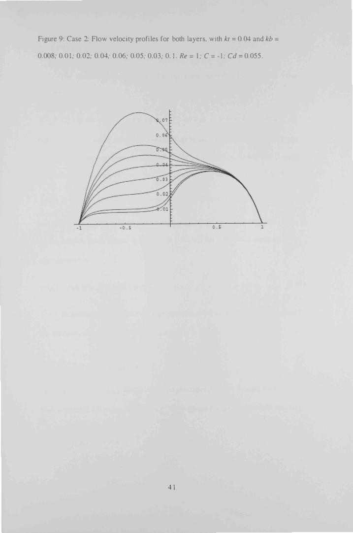
Figure 9 : Case 2: Flow veloci ty profi les for both layers, with kt = 0. 04 and kb =
0. 008; 0. 0 1 ,' 0. 02; 0. 04,' 0. 06; 0. 05,' 0.03; 0. 1 . Re = 1 ,' C = - 1 ,' Cd = 0. 055 .
1 . 07
4 1

5.2 FINITE D I FFERENCE APP ROACH
The fin i te di fference method for the linear second order boundary value
problem,
y" = p(x)y'+q(X) Y + rex), a ::; x ::; b, y (a) = a, y(b) = /3, (5 .28)
requires that difference quotient approximations be used to approximate both y' and
y " . First, we select an integer N > ° and divide the interval [a, b] into (N+ l ) equal
ubin tervals whose endpoints are the mesh poin ts x, = a + ih for i = 0, 1 , . . . . . , N + 1 ,
where h = b - a . Choosing the step s ize h in this manner faci l i tates the appl ication N + 1
of a matrix a lgori thm which sol ves a l inear system involving an N X N matrix [29] .
At the in terior mesh points, x, ' for i =O, I, . . . . . , N , the differential equation to be
approximated i s :
y" (X, ) = p(x; )y' (X, )+q(x, )y(x, )+ r(x, ), (5 . 29 )
Expanding y in a third Taylor polynomial about Xi and evaluated at XI+ I and
XI- I , we have, assuming that yE C4 [XI _ I , XI + I] ,
V" (XI) = J, [ y(xl + I ) - 2y(xl ) + y(xl _ I )] _ � y4 (�/ )' . h - 1 2 (5 .30 )
for some �, i n (X,_I ' x,+I ). This is cal led the centered difference fonnula for y" ( XI ) .
Then a centered difference formula for y'( xl ) i s obtained in a simi lar manner resul ting ln,
V' (XI ) = _1 [ y(xl + I ) - y(xl - I) _ h"
y" ' (T7, ) - 2h 6 (5 .3 1 )
42

for some '7, in (X,_I ' XI+I ) .
The use of these formulas in Equation (5 .29) results in the equation :
Y(XI + I) - 2y(xl ) + Y(XI - I ) [ Y(XI T I ) - Y(XI - I ) J -'-----'------=--h-=-2 --'---=--:'--'- = P (XI )
2h + q (XI ) Y (XI )
+ r(xl ) -�� [2p(xl ) y' " ('7, ) - l (�, ) J , (5 .32)
Define \\'0 = a , WN+I =/3
And
1 + 1 I 1-1 +p(x ) 1 + 1 I -I + q(x )W = - rex ) ( - w + 2 \V . - WW ) ( w - w ) 11 " I 2h I I I '
Rewrite this to get,
(5 .33)
(5 .34)
And the resulting system of equations is expressed in the tridiagonal N"X,N matrix
Aw=b,
Which i s a nonlinear system that can be solved by any i terative scheme for the
unknowns Wi.
43

5.3 THE NON LINEAR SHOOTING METHOD
The shooting technique for the nonl inear second order boundary value
problem
y" = I (x, y, y' ) , a � x � b, yea) = a, y(b) = (J, (5 .35)
i s s imilar to the l inear technique except that the solution to a nonlinear problem can
not be expressed as a linear combination of the solutions to the two initial value
problems. Instead, we approximate the sol ution to the boundary value problem by
using the solutions to a sequence of init ial value problems involving a parameter t.
these problems have the form
y" = I (x, y, y ' ) , a � x � b, y(a) = a, y ' (a) = t , (5 .36)
We do this by c hoosing t = t k ' in a manner to ensure that the I imit of y (b, t k )
as k goes to infin i ty equals y(b )= {J , where y (x, tk ) denotes the solution to the in i tial
value problem (5 . 36) with t = fk ' and y(x) denotes the solution to the boundary val ue
problem (5 . 35) .
Thi s technique i s cal led shooting method, by analogy to the procedure of
firing objects at a stationary target . We start with a parameter to that determines the
init ial elevation at which the object is fired from the poin t (a, a) and along the curve
described by the solution to the initial value problem (5 .36) .
44

If y(b, co ) i s not sufficiently close to p, we correct our approximation by choosing
elevations tl ' t 2 , and so on unti l y(b, lk ) is sufficiently close to hitting p [29] .
We next determine t with
y(b, t ) - fJ = O
Thi s i s a non linear equation and there are many methods avai lable to solve i t
such as the secant method. We j ust need to choose initial approximations to and t 1 , and
then generate the remaining terms of the sequence by
(y(b, lk - 1 ) - /3)(lk - 1 - lk - �) tk = tk - 1 - , k = 2,3, . . . . . y(b, £k - 1 ) - y(b, tk - ")
4 5

6.0 Fluid Flow through Mu lti layer of Finite Depth
In this section, we shal l present the mathematical formulations of the models
equations governing the three channel problem, where the middle region i s of fin i te
width H , and the upper and lower regions are of fin i te heights . The mathematical
formulations govern the flow of viscous fluid through porous media. The flow
through porous media has typically been described by Darcy's law which is only
suitable for s low flow through low permeabi l i ty media. Also, it ignores many physical
attri butes such as inertial effects and the viscous shear effects . When dealing with
viscous fluid flows and high permeabi l i ty medium, Darcy's law becomes not valid and
other flow models which account for these effects have to be adopted. Two popular
models are knowns as Darcy-Lapwood- B rinkman (DLB ) and the Darcy-Lapwood-
Forchheimer-Bri nkman (DFB ) models . The DLB model is suitable when viscous
shear effects are important and macroscopic inertia is sufficient to describe the flow
inertia through the porous materia l . The DFB model accounts for viscous shear
effects, and describes both microscopic and macroscopic inertia in the medium. The
flows described by these models are encountered in various natural , physical,
biological , and industrial settings.
If we assume that the flow i s planar, ful ly developed and driven by a constant
pressure gradient, then, in dimensionless form, the governing equation for the DFB
model i s
(6.0)
46

Where u (y ) , - 1 � Y � 1 , is the veloc i ty of the fluid, and the various parameters in
(6.0) are defined in terms of physical parameters as fol lows.
• Re = pU _ L is the Reynolds number with p is the fl uid density, Uoo is the Jl
free stream c haracteristic veloc i ty, �l is the fluid viscosity, and L i s the channel
characteri stic length .
• K i s the permeabi l i ty of the porous channe l .
• Cd is the fonn drag coefficient .
• C < 0 is a dimensionless pressure gradient.
When Cd = 0 , we obtain the DLB model equation
d 211 = Re C +!!.-dy '2 k ' (6 . 1 )
In this work, we consider flow through a channel composed of three different
porous layers . The upper ( lower) layer is bounded above (below) by a sol id
impermeable wal l , corresponding to y = - 2 and y = 1 . The y = 0 and y = - 1
correspond to the i nterface region . Since the upper (lower ) layer i s bounded above
(below) by sol i d impermeable wal l , a no slip condition is valid to assume, that is ,
u = 0 at the sol id boundaries y = - 2 and y = 1 . At the interface between the three
layers along y = 0 , - 1 , we assume that the veloc i ty and shear stress are continuous.
Thi s assumption is real istic and makes it possible to determine the fluid veloci ty at the
interface.
47

Then we apply the fini te difference method to solve the three layer flow
problem. The solution is approximated at grid point Y" and the solution u (O) , and its
derivative u ' (O) , at the interface are later approximated to be compared with the
imulation results of the non l inear shooting method.
_ _ _ _ _ _ _ _ _ _ _ _ In�r1"c:'" =;1 em _ _ _ _ _ _ _ _
Figure 1 0: Configuration of the three layer problem.
48

7.0 RESULTS A N D DISCUSS I O N
For our problem, w e assume that the flow is planar, fully developed, and
driven by a constant pressure gradient . We consider the flow through a channel which
is compo ed of three different porous layers . The flow through the layers i s governed
by two different flow models . The upper and lower layers are bounded by sol id,
impermeable wal ls on which a no slip condi tion i s val id. Near the sol id walls, strong
viscous shear effects are present, and hence one must choose a flow model that i s
compatible wi th the presence of macroscopic solid boundary. The interactions
between the fl uids in the three layers of the channel take place at the interface regions
between the porous layers. As a result , there will be a discontinui ty in the
permeabi l i ty at the i nterface due to the a ssumption that the interface between the
layers is sharp. In addition, across the interface, the momentum transfer and shear
stress effects are transmitted from the faster flow region to the slower flow region .
However, i t i s assumed that the velocity and shear stress are continuous along the
interface which makes it possible to determi ne the fluid veloc ity at the in terface .
The OFB (Darcy-Lapwood-Forchheimer-Brinkrnan) model is known to be
compatible wi th the presence of a macroscopic boundary. As a result, we choose the
OFB flow model to govern the top and bottom layer. Then, the governing equation for
the OFB model for the top and bottom layer i s :
(7.0)
Where u (y) , - 2 � y � - 1 and 0 � y � 1 , is the velocity of the fluid and the
various parameters in (7.0) are defined as fol lows:
49

• Re = pU _L is the Reynolds number with p is the fluid density, Drt, is the free JL
stream characteristic velocity, )l is the fluid viscosity, and L is the channel
characteristic length.
• K is the permeability of the porous channel.
• Cd is the form drag coefficient.
• C < 0 is a dimensionless pressure gradient.
The flow in the middle layer is governed by the DLB (Darcy-Lapwood-
Brinkman) model which has the following governing equation:
u u" = Re C + - , -1 � )' � O ,
km (7.1)
where km is the permeability associated with the middle layer. The permeabilities
are denoted by kl and kb for the upper and lower layers respectively. The
boundary conditions associated with the configuration above are as follows:
• Conditions along the solid walls: the no slip condition is employed at the
solid walls, thus
u (- 2) = 0 , and u(l) = 0
5 0
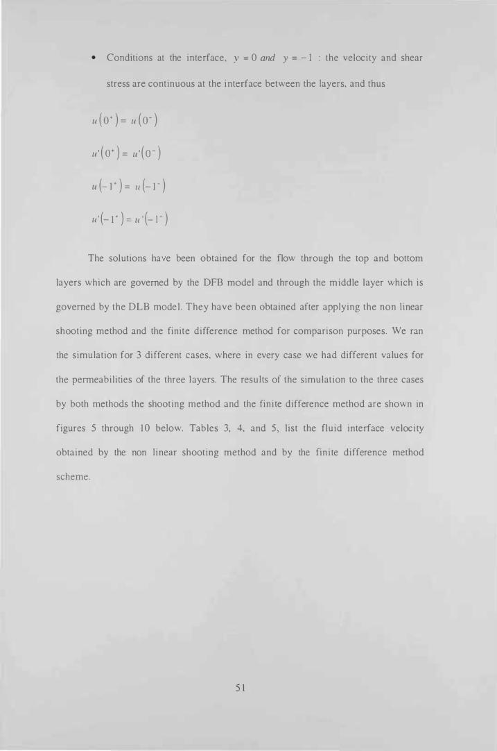
• Conditions at the interface, y = 0 and y = - 1 : the veloci ty and shear
stress are continuous at the interface between the layers, and thus
u ( o+ ) = u ( O- )
ll ' ( O+ ) = u ' ( O - )
U (_ 1 T ) = ll (- l - )
u ' (- l + ) = u ' (- l - )
The solutions ha e been obtained for the flow through the top and bottom
layers which are governed by the DFB model and through the middle layer which is
governed by the DLB mode l . They have been obtained after applying the non l inear
shooting method and the finite difference method for comparison purposes. We ran
the simulation for 3 different cases, where in every case we had different values for
the permeabil ities of the three layers. The resul ts of the simulation to the three cases
by both methods the shooting method and the fin i te difference method are shown in
figures 5 through 1 0 below. Tables 3, 4, and 5 l ist the flu id interface veloc i ty
obtained by the non l inear shooting method and by the fin i te difference method
scheme.
5 1

Table IV : Case I of the comparison between two methods : The
interface velocities for the alues : Kb= 0. 1 , Kc= 0.2, Kt= 1 0, a = -2, b= l c l = - 1 ,
c 2 = 0, R = 1 C = - 1 Cd = 0 . 1
Fi nite Shooting Method Difference Difference
U(m) 0. 143945 0. 14309 1 0.000854 U(2m) 0.278743 0.277 124 0.00 16 19
Table V : Case I I of the comparison between two methods : The
interface velocities for the values : Kb= 0. 1 , Kc= 0. 1 0, Kt= 1 0, a = -2, b= l , c 1 = - 1 ,
c 2 = 0, R = 1 , C = - 1 , C d = 0 . 1
Fin i te Shooting Method Difference Difference
U(m) 0.0994792 0.099396 0.0000832 U(2m) 0.1 94545 0. 19261 0.001935
5 2

Table VI : Case I I I of the comparison between two methods : The
interface veloci ties for the values: Kb= 0 .5 , Kc= 10, Kt= 0. 1 , a = -2, b= l , c 1 = - 1 ,
c2 = 0, R = 1 , C = - 1 , Cd = 0. 1
Finite Shooting Method Difference Di fference
U(m) 0.458824 0.458096 0.000728 U(2m) 0.286518 0.292454 0.005936
5 3

Iter. = 7
0.20
0 . 15
0 . 10
0.05
-2.0 - 1 .5 - 1 .0 -0.5 0.5 l .0
E_b = - 10 2.82029 10
Figure 1 1 : shooting method: With Kb= 0. 1 , Kc= 0 .2 , Kt= 1 0, a = -2 , b= l , c l = a + (b-a)/3, c2 = a + 2(b-a)/3
0.30 r
0.20
0.1 5
0.1 0
0.05
-2.0 - 1 .5 - 1 .0 -0.5 0.5 1 .0
Figure 1 2: fin i te difference method: With Kb= 0. 1 , Kc= 0.2, Kt= 1 0, a = -2 b= l , c 1 = a + (b-a)/3, c2 = a + 2(b-a)/3
54

Iter. = 7
.1 5
0. 10
0.05
-2.0 - l .5 - 1 .0 -0.5 0.5 1 .0
E_b = -10
4.3325 1 10
Figure 13 : shooting method: With Kb= 0. 1 , Kc= 0. 1 0, Kt= l a, a = -2 , b= l , c l = a +
(b-a)/3 , c2 = a + 2 (b-a)/3, R = 1 , C = - 1 , Cd = 0. 1
. 1 5
0 . 10
0.05
-2.0 - 1.5 - 1 .0 -0.5 0.5 l .0 Figure 1 4: Finite difference method: Kb= 0. 1 , Kc= 0. 1 0, Kt= 1 0, a = -2, b= l , c l = a + (b-a)/3, c2 = a + 2(b-a)/3, R = 1 , C = - 1 , Cd = 0. 1
55

Iter. = 20
0 .5
0.2
0 . 1
-2.0 - 1 .5 - 1 .0 -0.5 0.5 1 .0
E_b = - 10
4. 1 2895 1 0
Figure 1 5 : shooting method: With Kb= 0 . 5 , Kc= 1 0, Kt= 0. 1 , a = -2, b= l , c 1 = a + (ba)/3, c2 = a + 2(b-a)/3
0.5
0.4
0 . 1
-2 .0 - 1 .5 - l .0 -0 .5 0.5 l .0
Figure 1 6 : Finite difference method : With Kb= 0 .5 , Kc= 1 0, Kt= 0. 1 , a = -2, b= l c 1 = a + (b-a)/3 , c2 = a + 2(b-a)/3
5 6

The results of applying the shooting method to the three layer flow problem show
that the algori thm is more efficient and more accurate than the fin i te difference
method. In particu lar, we note that, in all cases, the interface veloc i ty and shear stress
values obtained by the fi nite di fference approach tend to the values obtained by the
shooting method. This demonstrates that the shooting method gives a better resolution
at the interface . The results show that the ve locity profi le is simi lar in al l three cases.
For the parameter values considered i n this work, the convergence of Newton's
method was very fast. In all cases considered, convergence was achieved in first and
second case in 7 i terations and for the third case in 20 i terations . On the other hand,
the finite difference method was time consuming as i t has to handle a large system.
57

C HA PTER EIGHT
8 .0 ENVI RONMENTAL I MPACT
Porous materials are encountered l i terally everywhere in everyday life , in
technology, and in nature . Many natural substances such as rocks, and biological
tissues such as lungs and bones, and man made materials such as cements, foams and
ceramics c an be considered as porous media. More examples of porous material
incl ude soil, bui lding materials such as bricks, concrete, l imestone, and sandstone.
The concept of porous media is used in many areas of appl ied science and
engineering . I t i s used in mechanics such as geo-mechanics, soi l and rock mechanics,
in engineering such as petroleum and construction engineering, in geosciences such as
hydrogeology and geophysics, in biology and biophysics, in material sciences, and
many more fields of science. However, the most important areas of technology that
depend s ign ificantly on the properties of porous media are hydrology, which re lates to
water movement in earth and sand structures, petroleum engineering which is mainly
concerned with petroleum, and natural gas production, exploration, well dri l l ing, and
logging. Additional ly, the flow of blood and other body fluids, and electro-osmosis
are few examples where porous media plays a critical role in medicine and biological
engi neering .
Consequently, flow through porous media has become an important
environmental problem that had attracted the attention of many scientists . It has many
environmental impl ications in several areas such as the study of pollution, fate of
contaminants, contaminations issues re lated to agricul ture, civi l constructions, coastal
management, and flow of ground water, oil and gas in the ground layers are also
5 8

typical problems. In addition, flow through porous media finds agricul tural
appl ications in irrigation processes and the movement of nutrients, ferti l izers, and
pol lutants into plants Fluid flow through porous media has emerged a separate field of
study because it is a subject of most common interest.
Differential equations play an important role in many fields of science and
engineering. They model many importan t physical phenomenon. In Fact, fluid
mechanics of the interface region of multilayer flows has gained interest over the past
three decades due to i ts applications in various physical settings . These appl ications
include packed bed heat exchangers, heat pipes thermal insulati on petroleum
reservoirs nuclear waste reposi tories, and geothermal engi neering [ 1 ] ,
In general, petroleum products represent a dangerous potential source of
groundwater pollu tion and sediment contamination due 0 the toxicity of a number of
the oi l components, such as benzene toluene, ethylene and xylene. These can reach
the water table through various pathways, inc luding highway runoff, direct oi l spi l l s
resulting from road accidents, wave washing of oi l spi l led in coastal waters, and the
improper disposal of hydrocarbon products through urban sewer systems.
Due to the costly c lean up processes of oi l contaminated sediments, i t is
imperative to predict the outreach of oi l components, their motion in the sediment, the
physical and chemical behavior of the redistributed oi l and how the oi l components
reach the water table . A l arge volume of work, both theoretical and experimental , has
been carried out in this fie ld in recent years and has been centered around a single and
mul tiphase flow through porous media [2 ] .
S 9

For example, organic tissues are porous media permeated by organic liquid.
They are made of packed ce l ls which constantly absorb organic material and nutrients
from the liquid environment outside them to feed, grow, and duplicate. On the other
hand, they constantly produce waste prod ucts, mainly water, and a multi tude of
chemical factors . At the end, when cel ls d ie , their membrane ruptures releasing their
content and in particular re-usable organic materials . One can then model these
bodies as growing and deformable porous media and study the fi l tration of organic
l iquids through them. Of course, this is not the only field which involves porous
media with mass exchanges. Other examples can be found in composite material
manufacturing, crystal l ization , petroleum and chemical engineering, glaciology,
sedimentation and erosion, contamination and decontamination of soi ls .
60

REFER ENCES
1 . ie ld, D . , Bej an , A. 1 999. Convection i n Porous Media. Springer: New York, 2nd
edi tion .
2 . Porous Media. (n . d.) Retrieved on November 26th, 2007, from :
http://www .fys .uio.no/-eaker/thesis/node5 . htrnl#SECTION004 1 0000000000000000
3 .Dul l ien F. (Feb 1 0 1 997) . Porous Media : Fluid Transport and Pore Structure .
Academics Porous Media. Retrieved on November 26lh, 2007, from:
http://www.fys. uio.no/-eaker/thesis/node5 . html#SECTION004 1 00000000000000003
4. Hansen, V .E . , Israelsen, O.W. ( 1 962) . Irrigation Principles and Practices. John
Wiley and Sons : New York, 3rd edition .
5 . Tiab, D . , Donaldson, E. ( 1 999). Theory and Practice of Measuring Reservoir Rock
and Fluid Transport Properties. Butterworth-Heinemann publ ished by the Gulf
Publ ishing Company, Houston, Tx.
6 . Verraij t, A. Groundwater Flow. The Macmi l lan Press : Hong kong, 2nd
edition .
7 . Dul len, F. ( 1 979) . Porous Media : Flui d Transport and Pore Structure . Academic
Press: New York.
8. Fredlund, D .G . , XING, A. (March 1 8 , 1 994). Predicting the permeabi l ity function
for unsaturated soi l s using the soi l -water. Retrieved on November 1 2, 2007, from:
http://www.soil vi sion .com/downloads/docs/pdf/research/cangeopredict. pdf
6 1

9 . Wal ter, T. , Gao, B . , Parlange, J . Y . (September 1 7 , 2007) . Modeling Soi l : Sol ute
Release into Runoff with Infi l tration . Science direct: Elsevier, Journal of Hydrology,
volume 347, is ues 3-4.
1 0. Saturated Hydraulic Conductivity. (n . d . ) Retrieved on November 1 2, 2007 from:
http://soi I s . usda.gov Itechnicalltechnotes/note6. html
1 1 . Water In Soi l . ( 1 997). Retrieved on November 1 2, 2007 from:
h ttp://www.css.comel l .edu/faculty/h mv l /watrsoil/wts l . htm
1 2 . Bouma, J. Brown R . B . (n .d . ) . Soi l as a Porous Medium. Retrieved on ovember
1 5 , 2007, from : http://edis. ifas.ufl . edulscripts/htmlgen.exe?DOCUMENT SS 1 08
1 3 . I srae lsen 0., Hansen, V . ( 1 962) . Irrigation Principles and Practices. John Wi ley
and sons: New York, 3rd edition .
1 4. ofziger D.L. (March 1 8 , 2003) . Water Movement in Soi ls . Retrieved on
ovember 1 2, 2007, from: http://soi lphysics .okstate .edulsoftware/waterlinfil .htrnl
1 5 . Soi l Structure . (November 5 , 2007) . W i kipedia: the free encyc lopedia. Retrieved
on ovember 1 2 , 2007 from : http://en .wikipedia.org/wiki/Soi l structure
1 6. Water Movement in Soi l . (n .d . ) . Retrieved on November 1 2, 2007, from:
h ttp://weather.nmsu.edu/teaching Material/soi I252/Chapl O.htm
1 7 . Trautmann N . , Porter, K. (n .d . ) . Water and the Soi l . Retrieved on November 1 5 ,
2007, from: http ://pmep.cce .comel l .edulfacts-slides-self/facts/wat -so-grw8S . h tml
62

1 8 . Watson, l , Hardy, L. (et a l ) . (September 1 995) . How Water Moves Through Soi l .
Rerrieved on ovember 1 51h , 2007 from :
http://cals.arizona.edu/pubs/water/az95 1 6 .pdf
1 9 . Physics of Porous Media. ( ovember 2 1 , 1 995) . Retrieved on November 261\ 2007 from : http://www.fys .uio.no/faststofflcoop/cop92/node29. h tml
20. Beavers, G.S . , Joseph, D .D . ( 1 967). Boundary conditions at a natural ly permeable
wal l . Journal of Fluid Mechanics, volume 30, issue 1 , pp. 1 97 .
2 1 . Be a ers, G .S . , Sparrow, E . M . and Masha, B .A . ( 1 974). Experiments of coupled
paral le l flows in a channel and a bounding porous medium. Applied Mathematics ,
volume 20, pp. 596 .
22. Vafai , K . , Thiyagaja , R . ( 1 987) . Analys is of flow and heat transfer at the interface
region of a porous medium. International journal of heat Mass and Transfer, Vol ume
30, pp 1 39 1 .
23. Vafai, K., Kim, S . J . ( 1 990). Fluid mechanics of the interface region between a
porous medium and a fluid layer: an exact solution . International journal of heat mass
and transfer, Volume 1 1 , i ssue 3 pp. 334.
24. Al lan , F., Hamdan, M . H . (2002). Fluid mechanics at the interface region between
two porous layers. Applied Mathematics Computations, Volume 1 28, Issue 1 , pp. 37 .
63

25 . olbakken S . , Andersson, H. (2005 . Direct numerical simulation of lubricated
channel flow. Fluid Dynamic Research, Volume 37, Issue 3, pp 203-230.
26. Lemos, M . , Renato, S. (2006) . Turbulent over a layer of a highly permeable
medium simulated with a diffusion jump m odel for the interface . International journal
of heat mass and transfer, ol ume 49, issues 3-4, pp. 546-556.
�7 . Allan, F. , Abu Ghniem, S . , Hasan, S . ( 2007) . Simple Mathematical Models for the
Fluid Flow through Channels . Preprin ts .
28 . Allan, F. Hajj i , M . A . , (2008) . Mathematical Manipulation of the Interface Region
of Multilayer Flow. International Journal of Porous Media (accepted).
29. Burden, R.L. and Faires, J .D . , (200 1 ) . Numerical Analysis. 7th ed. , Brooks/Cole.
30. Deeba, E., Khuri, S .A . and Xie, S. (2000). An A lgori thm for Solving Boundary
Value Problems, Journal of Computational Physics . vol . 5 59, pp. 1 25- 1 38 .
3 1 . Ford, R .A . , and Hamdan, M.H . , ( 1 998) . Coupled Parallel Flow Through
Composite Porous Layers. Applied Mathematics and Computations, vol . 97, pp. 26 1 -
27 1 .
32 . Charbeneau, R . (2000). Groundwater H ydraul ics and Pol lutant Transport]rentice
Hal l : New Jersey .
64

33 . Hwang, ., H i ta, C . ( 1 987). Fundamentals of Hydraul ic Engineering Systems.
Prentice Hal l : ew Jersey.
34. Verruij t, A. ( 1 982) . Theory of Groundwater Flow. The Macmil lan Press: London,
_ nd edition .
35 . Schwab, G . , Fangmeier, D. , Ell iot , W . ( 1 996) . Soil and Water Management
Systems . John Wi ley and sons: Toronto, 4th edition .
36. A l l an F. Hamdan, M.H. (2002). F lu id Mechanics of The Interface Region
Between Two porous Layers. Applied Mathematics Computation, vol . 1 28 , no. 1 , pp.
37-43 .
37. Rudraiah, N. ( 1 986) . Flow Past Porous Layers and Their Stabi lity. Encyclopedia
of Fluid Mechanics, S l urry Flow Technology, ch . 14 .
38 . Assher, UM. , Matthij , R .M.M. , and Russel R .D. ( 1 995) . Numerical solution of
boundary val ue problems for ordinary differential equations . Society for industrial
and Applied Mathematics, Phi ladelphia, PA .
39. B . C . Chandra Sekhara, K . Rajani, N . Rudraiah. ( 1 987) . Effect of sl ip on porous
walled squeeze fi lms in the presence of a magnetic field . Appl . Sci . Res . Vol ume 34,
pp. 393 .
40. Verwoerd, W.S . (February 2009) . New stochastic model for dispersion in
heterogeneous porous media: Application to unbounded domains. Applied
Mathematical Model l ing, Volume 33, Issue 2 , Pages 605-625 .
65

4 1 . Karim, M. , Tanimoto, K . , and Hieu , P. D. (January 2009) . Modell ing and
simulation of wave transformation in porous structures using VOF based two-phase
flow mode l . Applied Mathematical Mode l l ing, Vol ume 33 Issue 1 , January 2009
Pages 343-360.
42. Reckner, M. Wang, F .Y. (December 1 5 , 2008). Non-monotone stochastic
general ized porous media equations . Journal of Di fferential Equations, Volume 245 ,
Issue 1 2, Pages 3898-3935 .
43 . A . Ramirez, A. Romero, F. Chavez, F . Carri l lo, S . Lopez. ( ovember 2008) .
Mathematical simulation of oil reservoir properties. Chaos, Solitons &
Fractals , Volume 38, Issue 3, Pages 778-788 .
44. Polubarinova K . ( 1 960) . Theory of Groundwater Movement, Princeton Uni versity
Press, Princeton NJ.
45. Harr, M. ( 1 962). Groundwater and Seepage. McGraw Hi l l , New York.
46. Awartani , M.M. , Hamdan, M . H . (2005 ) . Ful ly developed flow through a porous
channel bounded by flat plates. Applied M athematics, volume 1 69, pp. 749.
47. M. Khan, Ehnber Naheed, C . Fetecau, T. Hayat. (November 2008). Exact
solutions of starting flows for second grade fluid in a porous medium.
International Journal of Non-Linear Mechanics, Volume 43, Issue 9, Pages 868-879
66

U AEU LI BRARY
IIIIIII illllll\ II\i IIIII IIIII I�I IIIII IIIII IIIII I� IIII 1 000456956


o�1 �yJI WI)_A I �� 4WI w�IJ�1 o..)L..c.
�I _ 1- � La . \� . f'� � � Y.
�I
2008


