
Flexible Specification of Large Systems ofNonlinear PDEs
Hans Petter Langtangen1,2 Mikael Mortensen3,1
Center for Biomedical Computing
Simula Research Laboratory1
Dept. of Informatics, University of Oslo2
Dept. of Mathematics, University of Oslo3
[HPC]3 at KAUST, Feb 6, 2012

FEniCS PDE tools
PDE systems toolsand CFD

1 FEniCS PDE tools
2 PDE system tools and CFD

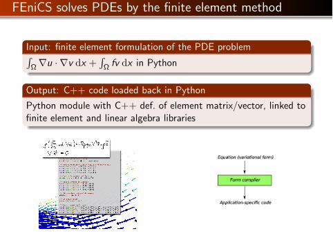
FEniCS solves PDEs by the finite element method
Input: finite element formulation of the PDE problemΩ∇u ·∇v dx +
Ωfv dx in Python
Output: C++ code loaded back in Python
Python module with C++ def. of element matrix/vector, linked tofinite element and linear algebra libraries

FEniCS solves PDEs by the finite element method
Input: finite element formulation of the PDE problemΩ∇u ·∇v dx +
Ωfv dx in Python
Output: C++ code loaded back in Python
Python module with C++ def. of element matrix/vector, linked tofinite element and linear algebra libraries
FEniCS solves PDEs by the finite element method
Input: finite element formulation of the PDE problemΩ∇u ·∇v dx +
Ωfv dx in Python
Output: C++ code loaded back in Python
Python module with C++ def. of element matrix/vector, linked tofinite element and linear algebra libraries

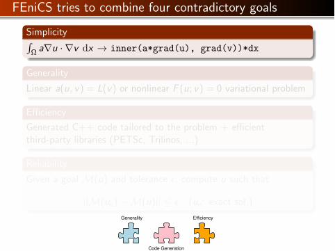
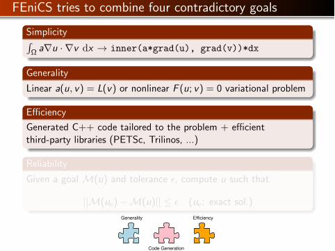
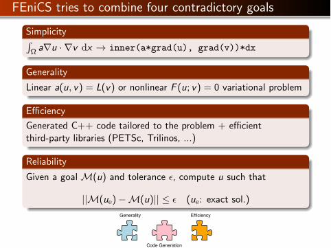
FEniCS tries to combine four contradictory goals
SimplicityΩa∇u ·∇v dx → inner(a*grad(u), grad(v))*dx
Generality
Linear a(u, v) = L(v) or nonlinear F (u; v) = 0 variational problem
Efficiency
Generated C++ code tailored to the problem + efficientthird-party libraries (PETSc, Trilinos, ...)
Reliability
Given a goal M(u) and tolerance , compute u such that
||M(ue)−M(u)|| ≤ (ue: exact sol.)
Generality Efficiency
Code Generation
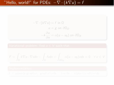
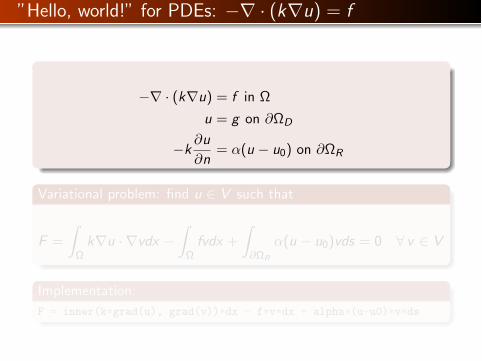
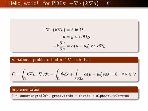
”Hello, world!” for PDEs: −∇ · (k∇u) = f

”Hello, world!” for HPC3: ut +∇ · F (u) = 0
”Hello, world!” for PDEs: −∇ · (k∇u) = f
−∇ · (k∇u) = f in Ω
u = g on ∂ΩD
−k∂u
∂n= α(u − u0) on ∂ΩR
Variational problem: find u ∈ V such that
F =
Ω
k∇u ·∇vdx −
Ω
fvdx +
∂ΩR
α(u − u0)vds = 0 ∀ v ∈ V
Implementation:
F = inner(k*grad(u), grad(v))*dx - f*v*dx + alpha*(u-u0)*v*ds
”Hello, world!” for PDEs: −∇ · (k∇u) = f
−∇ · (k∇u) = f in Ω
u = g on ∂ΩD
−k∂u
∂n= α(u − u0) on ∂ΩR
Variational problem: find u ∈ V such that
F =
Ω
k∇u ·∇vdx −
Ω
fvdx +
∂ΩR
α(u − u0)vds = 0 ∀ v ∈ V
Implementation:
F = inner(k*grad(u), grad(v))*dx - f*v*dx + alpha*(u-u0)*v*ds

”Hello, world!” for PDEs: −∇ · (k∇u) = f
−∇ · (k∇u) = f in Ω
u = g on ∂ΩD
−k∂u
∂n= α(u − u0) on ∂ΩR
Variational problem: find u ∈ V such that
F =
Ω
k∇u ·∇vdx −
Ω
fvdx +
∂ΩR
α(u − u0)vds = 0 ∀ v ∈ V
Implementation:
F = inner(k*grad(u), grad(v))*dx - f*v*dx + alpha*(u-u0)*v*ds
”Hello, world!” for PDEs: −∇ · (k∇u) = f
−∇ · (k∇u) = f in Ω
u = g on ∂ΩD
−k∂u
∂n= α(u − u0) on ∂ΩR
Variational problem: find u ∈ V such that
F =
Ω
k∇u ·∇vdx −
Ω
fvdx +
∂ΩR
α(u − u0)vds = 0 ∀ v ∈ V
Implementation:
F = inner(k*grad(u), grad(v))*dx - f*v*dx + alpha*(u-u0)*v*ds
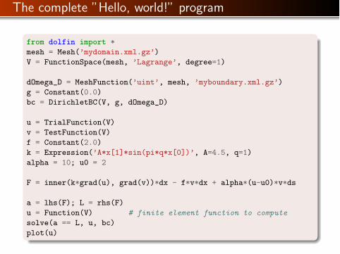
The complete ”Hello, world!” program
from dolfin import *
mesh = Mesh(’mydomain.xml.gz’)
V = FunctionSpace(mesh, ’Lagrange’, degree=1)
dOmega_D = MeshFunction(’uint’, mesh, ’myboundary.xml.gz’)
g = Constant(0.0)
bc = DirichletBC(V, g, dOmega_D)
u = TrialFunction(V)
v = TestFunction(V)
f = Constant(2.0)
k = Expression(’A*x[1]*sin(pi*q*x[0])’, A=4.5, q=1)
alpha = 10; u0 = 2
F = inner(k*grad(u), grad(v))*dx - f*v*dx + alpha*(u-u0)*v*ds
a = lhs(F); L = rhs(F)
u = Function(V) # finite element function to compute
solve(a == L, u, bc)
plot(u)
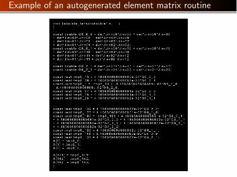
Example of an autogenerated element matrix routine

Mixed formulation of −∇ · (k∇u) = f
PDE problem:
∇ · q = f in Ω
−k−1q = ∇u in Ω
Variational problem: find (u, q) ∈ V × Q such that
F =
Ω
∇ · q v dx −
Ω
fv dx +
Ω
k−1q · p dx +
Ω
∇ · p u dx
∀ (v , p) ∈ V × Q
Principal implementation line:
F = div(q)*v*dx - f*u*dx + (1./k)*inner(q,p)*dx + div(p)*u*dx
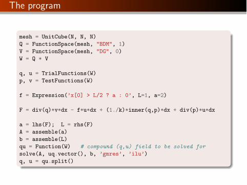
The program
mesh = UnitCube(N, N, N)
Q = FunctionSpace(mesh, "BDM", 1)
V = FunctionSpace(mesh, "DG", 0)
W = Q * V
q, u = TrialFunctions(W)
p, v = TestFunctions(W)
f = Expression(’x[0] > L/2 ? a : 0’, L=1, a=2)
F = div(q)*v*dx - f*u*dx + (1./k)*inner(q,p)*dx + div(p)*u*dx
a = lhs(F); L = rhs(F)
A = assemble(a)
b = assemble(L)
qu = Function(W) # compound (q,u) field to be solved for
solve(A, uq.vector(), b, ’gmres’, ’ilu’)
q, u = qu.split()
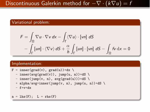
Discontinuous Galerkin method for −∇ · (k∇u) = f
Variational problem:
F =
Ω
∇u ·∇v dx −
Γ
∇u · [vn] dS
−
Γ
[un] · ∇v dS +α
h
Γ
[un] · [vn] dS −
Ω
fv dx = 0
Implementation:
F = inner(grad(v), grad(u))*dx \
- inner(avg(grad(v)), jump(u, n))*dS \
- inner(jump(v, n), avg(grad(u)))*dS \
+ alpha/avg*inner(jump(v, n), jump(u, n))*dS \
- f*v*dx
a = lhs(F); L = rhs(F)
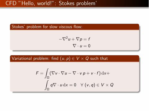
CFD ”Hello, world!”: Stokes problem’
Stokes’ problem for slow viscous flow:
−∇2u +∇p = f
∇ · u = 0
Variational problem: find (u, p) ∈ V × Q such that
F =
Ω
(∇v ·∇u −∇ · v p + v · f ) dx+
Ω
q∇ · u dx = 0 ∀ (v , q) ∈ V × Q
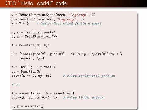
CFD ”Hello, world!” code
V = VectorFunctionSpace(mesh, ’Lagrange’, 2)
Q = FunctionSpace(mesh, ’Lagrange’, 1)
W = V * Q # Taylor-Hood mixed finite element
v, q = TestFunctions(W)
u, p = TrialFunctions(W)
f = Constant((0, 0))
F = (inner(grad(v), grad(u)) - div(v)*p + q*div(u))*dx + \
inner(v, f)*dx
a = lhs(F); L = rhs(F)
up = Function(W)
solve(a == L, up, bc) # solve variational problem
# or
A = assemble(a); b = assemble(L)
solve(A, up.vector(), b) # solve linear system
u, p = up.split()

Again, code ≈ math
Key mathematical formula:
F =
Ω
(∇v ·∇u −∇ · v p + v · f ) dx +
Ω
q∇ · u dx
Key code line:
F = (inner(grad(v), grad(u)) - div(v)*p + inner(f,v)*dx + \
q*div(u))*dx
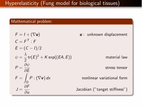
Hyperelasticity (Fung model for biological tissues)
Mathematical problem:
F = I + (∇uuu) uuu : unknown displacement
C = FT : F
E = (C − I )/2
ψ =λ
2tr(E )2 + K exp((EA,E )) material law
P =∂ψ
∂Estress tensor
F =
Ω
P : (∇vvv) dx nonlinear variational form
J =∂F
∂uJacobian (”tanget stiffness”)
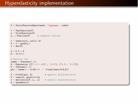
Hyperelasticity implementation
V = VectorFunctionSpace(mesh, ’Lagrange’, order)
v = TestFunction(V)u = TrialFunction(V)u_ = Function(V) # computed solution
I = Identity(u_.cell().d)F = I + grad(u_)J = det(F)
C = F.T * FE = (C-I)/2
# Material law
lamda = Constant(1.0)A = Expression ([[’1.0 + x[0]’, ’0.3’], [’0.3’, ’2.3’]])K = Constant(1.0)psi = lamda/2 * tr(E)**2 + K*exp(inner(A*E,E))
P = F*diff(psi, E) # symbolic differentiation
F = inner(P, grad(v))*dxJ = derivative(F, u_, u) # symbolic differentiation
A = assemble(J)
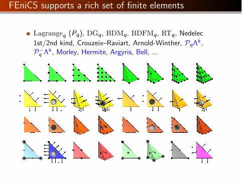
FEniCS supports a rich set of finite elements
Lagrangeq (Pq), DGq, BDMq, BDFMq, RTq, Nedelec
1st/2nd kind, Crouzeix–Raviart, Arnold-Winther, PqΛk ,P−q Λk , Morley, Hermite, Argyris, Bell, ...

Parallel computing
Distributed computing via MPI:mpirun -n 32 python myprog.py
Shared memory via OpenMP:# In program
parameters[’num_threads’] = Q

Automated error control
Input
a(u, v) = L(v) orF (u; v) = 0
Goal M(u)
> 0
Output
u such that
M(ue)−M(u) ≤
(ue: exact solution)

FEniCS automatatically generates a posteriori errorestimators and refinement indicators
Solve
Dual Estimate
uh
Indicate
Refine
ηTT∈Th
ηh <
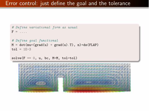
Error control: just define the goal and the tolerance
# Define variational form as usual
F = ....
# Define goal functional
M = dot(mu*(grad(u) + grad(u).T), n)*ds(FLAP)
tol = 1E-3
solve(F == 0, u, bc, M=M, tol=tol)

Example: compute shear stress in a bone implant
Polymer-fluid mixture
Nonlinear hyperelasticity
Complicated constitutive law
Novel mixeddisplacement-stressdiscretization viaArnold-Winther element
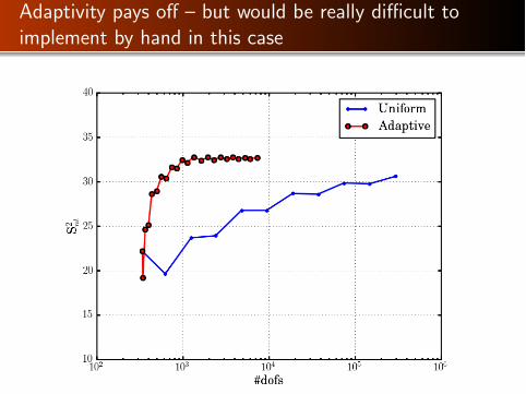
Adaptivity pays off – but would be really difficult toimplement by hand in this case

fenicsproject.org

FEniCS is easy to install
Easiest on Ubuntu (Debian):sudo apt-get install fenics
Mac OS X drag and drop installation (.dmg file)
Windows binary installer
Automated installation from source (compile & link)

FEniCS is a multi-institutional project
Initiated 2003 by Univ. of Chicago and Chalmers Univ. ofTechnology (Ridgway Scott and Claes Johnson)
Important contributions fromUniv.of Chicago (Rob Kirby, Andy Terrel, Matt Knepley, R. Scott)Chalmers Univ. of Technology (Anders Logg, Johan Hoffman,Johan Janson)Delft Univ. of Technology (Garth Wells, Kristian Oelgaard)
Current key institutions:Simula Research Laboratory (Anders Logg, Marie Rognes, MartinAlnæs, Johan Hake, Kent-Andre Mardal, ...)Cambridge University (Garth Wells, ...)
About 20 active developers
Lots of application developers

1 FEniCS PDE tools
2 PDE system tools and CFD
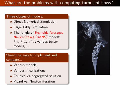
What are the problems with computing turbulent flows?
Three classes of models:
Direct Numerical Simulation
Large Eddy Simulation
The jungle of Reynolds-AveragedNavier-Stokes (RANS) models:k-, k-ω, v2-f , various tensormodels, ...
Should be easy to implement andcompare...
Various models
Various linearizations
Coupled vs. segregated solution
Picard vs. Newton iteration
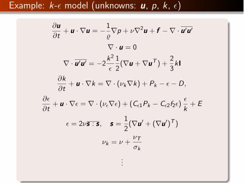
Example: k- model (unknowns: uuu, p, k , )
∂uuu
∂t+ uuu ·∇uuu = −1
∇p + ν∇2uuu + fff −∇ · uuuuuu
∇ · uuu = 0
∇ · uuuuuu = −2k2
1
2(∇uuu +∇uuuT ) +
2
3kI
∂k
∂t+ uuu ·∇k = ∇ · (νk∇k) + Pk − − D,
∂
∂t+ uuu ·∇ = ∇ · (ν∇) + (C1Pk − C2f2)
k+ E
= 2νsss : sss, sss =1
2(∇uuu + (∇uuu)T )
νk = ν +νTσk
...
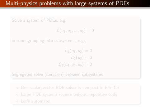
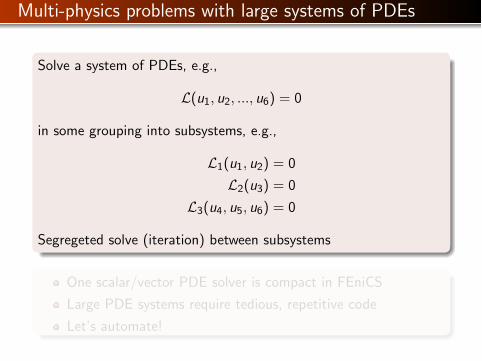
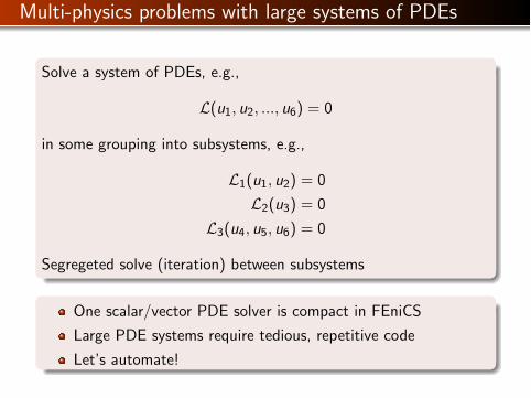
Multi-physics problems with large systems of PDEs
Solve a system of PDEs, e.g.,
L(u1, u2, ..., u6) = 0
in some grouping into subsystems, e.g.,
L1(u1, u2) = 0
L2(u3) = 0
L3(u4, u5, u6) = 0
Segregeted solve (iteration) between subsystems
One scalar/vector PDE solver is compact in FEniCS
Large PDE systems require tedious, repetitive code
Let’s automate!

Download from launchpad.net: bzr branch lp:cbcpdesys

Principles for solving a system of PDEs L(u1, u2, ...) = 0
List the names of unknowns: u1, u2, ...
Automatically create standard FEniCS objects:FunctionSpace V_u1 (mesh, element_u1, degree_u1)
Function u1_ (V_u1)
TrialFunction u1 (V_u1)
TestFunction v_u1 (V_u1)
Let the user supply the form:inner(u1*grad(u2), grad(v_u2)) ...
Let the user specify degree of implicitness:[[’u1’, ’u2’], [’u3’], [’u4’, ’u5’, ’u6’]]
= 3 PDE systems: 2× 2, scalar, 3× 3
Automatically create mixed function spaces, linear systems,Jacobians, call up nonlinear solves, etc.
Easy to optimize (precomputed matrices, etc.)

What needs to be programmed by a user?
Name the unknowns
Problem instance containing problem-specific parameters
PDESystem instance with list of unknowns grouped intosubsystems
For each subsystem, a PDESubSystem subclass with methodform to specify a variational formclass NavierStokes(PDESubSystem):
def form(self, u, v_u, u_, u_1, p, v_p, nu, dt, f,
**kwargs):
return (1/dt)*inner(u - u_1, v_u)*dx + \
inner(u_1*nabla_grad(u_1), v_u) + \
nu*inner(grad(u), grad(v_u))*dx - \
inner(p, div(v_u))*dx + inner(div(U), v_p)*dx

Inner details & ideas
The user defines the notation (names of unknowns + forms)
The library must be general
Callbacks to the user must have argument namescorresponding to the user’s notation
No classical code generation (just Python)
Heavy use of string operations, eval and **kwargs
Store data as dicts (and attributes for convenience)
Send the namespaces (user’s and generated) around
Rely on simple naming conventions: u, u , v k, V u, ...

Currently implemented solvers for CFD
Navier-Stokes solvers
Fully coupled
SegregatedChorinIncremental pressure correction
RANS models
Spalart-Allmaras
k − Low-Reynolds modelsStandard k −
v2 − f modelOriginalLien-Kalizin
Elliptic relaxationLRR-IPSSG

A k equation in a turbulence model
PDE for turbulent kinetic energy k (unknowns: u, k , )
0 = −u ·∇k +∇ · (νk(u, k , )∇k) + Pk(u, k , )−
Typical linearization (underscore subscript: old value)
0 = −u− ·∇k +∇ · (νk−∇k) + Pk− −

Variational form and Python code: code ≈ math
Variational form (k and vk are trial and test functions)
Fk = −
Ω
u− ·∇k vk dx −
Ω
νk−∇k ·∇vk dx +
Ω
(Pk−− ) vk dx
Corresponding code
F_k = - inner(dot(u_, grad(k)), v_k)*dx \
- nu_k_*inner(grad(k), grad(v_k))*dx \
+ (P_k_ - e)*v_k*dx

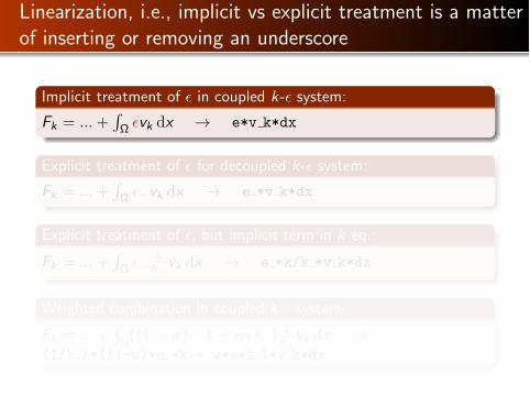
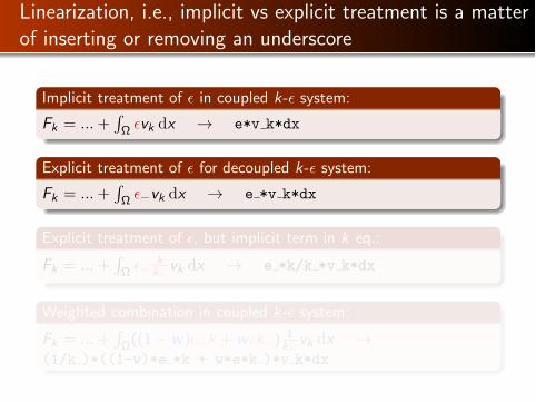
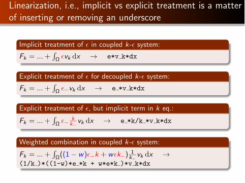
Linearization, i.e., implicit vs explicit treatment is a matterof inserting or removing an underscore
Implicit treatment of in coupled k- system:
Fk = ...+Ωvk dx → e*v k*dx
Explicit treatment of for decoupled k- system:
Fk = ...+Ω−vk dx → e *v k*dx
Explicit treatment of , but implicit term in k eq.:
Fk = ...+Ω−
kk−
vk dx → e *k/k *v k*dx
Weighted combination in coupled k- system:
Fk = ...+Ω((1− w)−k + wk−)
1
k−vk dx →
(1/k )*((1-w)*e *k + w*e*k )*v k*dx
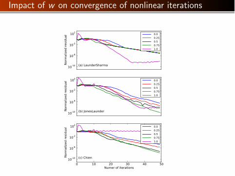
Impact of w on convergence of nonlinear iterations
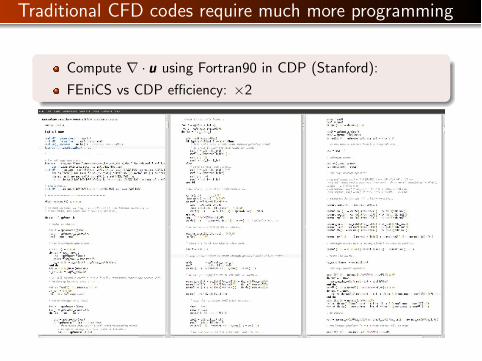
Traditional CFD codes require much more programming
Compute ∇ · uuu using Fortran90 in CDP (Stanford):
FEniCS vs CDP efficiency: ×2
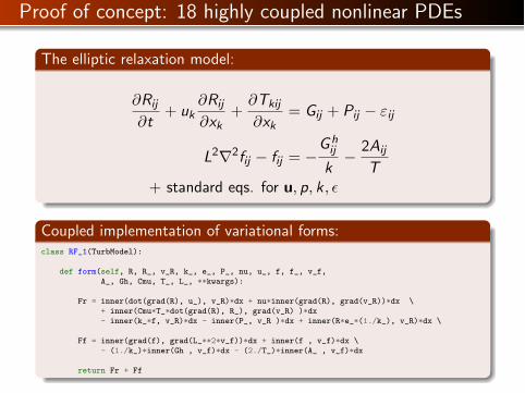
Proof of concept: 18 highly coupled nonlinear PDEs
The elliptic relaxation model:
∂Rij
∂t+ uk
∂Rij
∂xk+
∂Tkij
∂xk= Gij + Pij − εij
L2∇2fij − fij = −Ghij
k−
2Aij
T+ standard eqs. for u, p, k ,
Coupled implementation of variational forms:class RF_1(TurbModel):
def form(self, R, R_, v_R, k_, e_, P_, nu, u_, f, f_, v_f,A_, Gh, Cmu, T_, L_, **kwargs):
Fr = inner(dot(grad(R), u_), v_R)*dx + nu*inner(grad(R), grad(v_R))*dx \+ inner(Cmu*T_*dot(grad(R), R_), grad(v_R) )*dx- inner(k_*f, v_R)*dx - inner(P_, v_R )*dx + inner(R*e_*(1./k_), v_R)*dx \
Ff = inner(grad(f), grad(L_**2*v_f))*dx + inner(f , v_f)*dx \- (1./k_)*inner(Gh , v_f)*dx - (2./T_)*inner(A_ , v_f)*dx
return Fr + Ff

Diffusor as validation problem
Consider a diffusor with flow through an expanding channel:
Reτ = 395
Separation and recirculation
Elliptic relaxation model

Redistribution parameter Reynolds stresses
Ongoing work: libraries built on FEniCS
Uncertainty quantification: (generalized) multivariatepolynomial chaos with dependent variables
non-intrusiveintrusive (new PDEs :-)
PDE constrained optimization for inverse problems(define Lagrangian, autogenerate the rest)
Block preconditioning
Automated adaptive time integration for PDEs
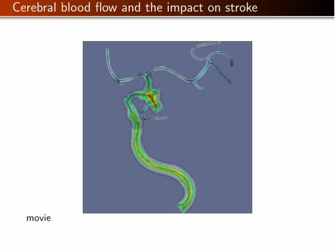
Cerebral blood flow and the impact on stroke
movie

Summary
Follow links and read more
FEniCS: Python FEM mathsyntax with HPC
pdesys package: flexiblesyntax for PDE systems
Vast collection of CFDsolvers
More info
The FEniCS tutorial
The FEniCS book onlaunchpad.net and Springer
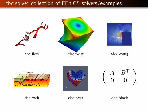
cbc.solve: collection of FEniCS solvers/examples
cbc.flow cbc.twist cbc.swing
cbc.rock cbc.beat cbc.block
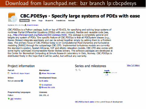
Download from launchpad.net: bzr branch lp:cbcpdesys


