
FLEXIBLE INFLATION TARGETS, FOREX INTERVENTIONS AND EXCHANGE RATE VOLATILITY IN EMERGING COUNTRIES
Juan Carlos Berganza and Carmen Broto
Documentos de Trabajo N.º 1105
2011

FLEXIBLE INFLATION TARGETS, FOREX INTERVENTIONS AND EXCHANGE RATE
VOLATILITY IN EMERGING COUNTRIES
FLEXIBLE INFLATION TARGETS, FOREX INTERVENTIONS
AND EXCHANGE RATE VOLATILITY IN EMERGING COUNTRIES
Juan Carlos Berganza and Carmen Broto (*)
BANCO DE ESPAÑA
(*) Contact authors: [email protected]; [email protected]. We thank Esther López for excellent assistance with the databases and Enrique Alberola, Raquel Carrasco, Luis Molina, Juan Ruiz and José María Serena for their helpful comments. We also thank seminar participants at Banco de España, the XXXV Simposio de Análisis Eco-nómico (Madrid), VIII ESCB workshop on EMEs (Saariselkä, Finland) and XV CEMLA conference (La Paz, Bolivia). The opinions expressed in this document are solely responsibility of the authors and do not represent the views of the Banco de España.
Documentos de Trabajo. N.º 1105
2011

The Working Paper Series seeks to disseminate original research in economics and fi nance. All papers have been anonymously refereed. By publishing these papers, the Banco de España aims to contribute to economic analysis and, in particular, to knowledge of the Spanish economy and its international environment.
The opinions and analyses in the Working Paper Series are the responsibility of the authors and, therefore, do not necessarily coincide with those of the Banco de España or the Eurosystem.
The Banco de España disseminates its main reports and most of its publications via the INTERNET at the following website: http://www.bde.es.
Reproduction for educational and non-commercial purposes is permitted provided that the source is acknowledged.
© BANCO DE ESPAÑA, Madrid, 2011
ISSN: 0213-2710 (print)ISSN: 1579-8666 (on line)Depósito legal: M. 17229-2011Unidad de Publicaciones, Banco de España
Abstract
Emerging economies with infl ation targets (IT) face a dilemma between fulfi lling the theoretical
conditions of “strict IT”, which imply a fully fl exible exchange rate, or applying a “fl exible IT”,
which entails a de facto managed fl oating exchange rate with FX interventions to moderate
exchange rate volatility. Using a panel data model for 37 countries we fi nd that, although IT
lead to higher exchange rate instability than alternative regimes, FX interventions in some
IT countries have been more effective to lower volatility than in non-IT countries, which may
justify the use of “fl exible IT” by policymakers.
Keywords: Infl ation targeting; Exchange rate volatility; Foreign exchange interventions;
Emerging economies.
JEL classifi cation: E31; E42; E52; E58; F31.

Resumen
Las economías emergentes con metas de infl ación (MI) se enfrentan a un dilema entre
cumplir las condiciones teóricas de una «MI estricta», lo que implica un tipo de cambio
totalmente fl exible, o seguir una gestión más activa de su moneda («MI fl exible»), lo que
supone implementar intervenciones cambiarias para moderar su volatilidad. Utilizando un
modelo de datos de panel para 37 países, mostramos que, a pesar de que las MI implican
una mayor inestabilidad del tipo de cambio que regímenes alternativos, las intervenciones
realizadas por algunos países con MI han sido más efi caces para reducir la volatilidad que
aquellas de países sin MI. Este resultado puede justifi car la utilización de «MI fl exibles» por
parte de los bancos centrales.
Palabras claves: Metas de infl ación, volatilidad del tipo de cambio, intervenciones
cambiarias, economías emergentes.
Códigos JEL : E31; E42; E52; E58; F31.

BANCO DE ESPAÑA 9 DOCUMENTO DE TRABAJO N.º 1105
1 Introduction
Since New Zealand adopted an inflation target (IT hereafter) in 1990, an increasing num-
ber of countries have implemented this monetary policy framework. According to IMF
(2005) and Little and Romano (2009), after Israel adopted its IT in 1997, 18 emerg-
ing countries (EMEs onwards) have changed their exchange rate regime (from fixed to
floating) and their nominal anchor (from exchange rate to inflation). See Table 1 for a
summary of IT adoption dates in EMEs. Although the effectiveness of IT to lower the
inflation level and volatility still remains controversial,1 this framework has been more
durable than other monetary policy strategies (Mihov and Rose, 2008). One of the main
reasons for this is that IT countries have benefited from the credibility gains from ex-
plicitly announcing the target, which helped to anchor and lower inflation expectations
(Mishkin and Schmidt-Hebbel, 2007).2
A flexible nominal exchange rate constitutes, at least from a theoretical standpoint, a
requirement for a well functioning full-fledged IT regime (Mishkin and Savastano, 2001).
Its rationale is based on the policy dilemma of the “impossibility of the Holy Trinity",
as in a context of capital mobility, an independent monetary policy cannot be combined
with a fixed exchange rate or a peg to another currency through interventions in the
foreign exchange markets (also known as forex or FX interventions); see Obstfeld et
al. (2005). Some economists state that one of the costs of IT is precisely the higher
volatility of exchange rates as a result of the floating exchange rate regime, which can
entail negative effects of particular relevance for EMEs given their greater financial and
real vulnerabilities (Cavoli, 2009). In fact, this is the basis of the “fear of floating" (Calvo
and Reinhart, 2002), which is a phenomenon mostly associated to EMEs.3 Accordingly,
1See Ball and Sheridan (2005) or Brito and Bystedt (2010) for some empirical evidence against the
positive role of IT in developed and emerging countries, respectively.2This effect is even stronger in EMEs, as their initial credibility is lower than that of developed
countries (Gonçalves and Salles, 2008).3According to Cavoli (2009), the main reasons to justify the “fear of floating" are: (i) trade contraction
–higher exchange rate volatility will discourage other countries to engage trade–; (ii) a higher pass-
through from exchange rate to domestic prices in EMEs than in developed countries; and, (iii) balance
sheet effects provoked by currency mismatches (liability dollarization).
BANCO DE ESPAÑA 10 DOCUMENTO DE TRABAJO N.º 1105
during economic booms EMEs also experience “fear of appreciation" given their concerns
for their loss of competitiveness (Levy-Yeyati and Sturzenegger, 2007).
Thus, exchange rate monitoring under IT poses some challenges for EMEs that dif-
fer from those in advanced economies. This might justify their more active role of the
exchange rate policies–particularly in those countries where the exchange rate has pre-
viously played a key role as nominal anchor–despite the theoretical reservations about
it. Consequently, in practice, EMEs with IT generally have less flexible exchange rate
arrangements, intervene more frequently in foreign exchange markets than their advanced
economy counterparts and have a greater response to real exchange rate movements (see
Aizenmann et al., 2008, and Chang, 2008).4
This adaptive way of implementing IT has been called “flexible IT" and it has gen-
erated an intense debate about its validity and viability in EMEs, compared with “strict
or pure IT", where the exchange rate does not enter in the reaction function of central
banks.5 That is, implicitly there is a policy dilemma between fulfilling the theoretical
requirements of IT and strictly follow it, or applying a “flexible IT", in the sense of using
FX interventions to smoothen the exchange rate volatility.
To this respect, there are different views in the literature. On the one hand, some
authors like Bernanke et al. (1999) hold that attending to IT and reacting to the ex-
change rate are mutually exclusive as FX interventions could confuse the public about the
priorities of the central bank, which distorts expectations. On the other hand, less strict
authors argue that central banks might interfere with the exchange rate volatility. For
instance, according to Cordero (2009), FX interventions are fully justified, as far as EMEs
need to maintain stable and competitive real exchange rates. In fact, following Taylor
(2000), some authors include the exchange rate in the policy reaction function arguing
that it helps to mitigate the impact of shocks, by dampening exchange rate volatility
4In contrast to EMEs, the most common reason to perform FX interventions in IT advanced economies
is to correct an exchange rate misalignment (Stone et al., 2009). In EMEs, there are other reasons to
intervene, apart from moderating the exchange rate volatility (for instance, to influence on the exchange
rate or to accumulate reserves).5The term “flexible", as defined in Svensson (2010), refers to IT central banks that look, not only for
price stability, but also consider other variables, such as the output gap or the exchange rate.
BANCO DE ESPAÑA 11 DOCUMENTO DE TRABAJO N.º 1105
(Kirnasova et al., 2006; Cavoli, 2008).
Other papers reach halfway conclusions about the role of exchange rates in IT regimes
from a more theoretical point of view. For instance, Stone et al. (2009) show that it
depends on the structure of the economy, the nature of the shocks, and the way in which
the exchange rate enters the policy rule. In the same line, Parrado (2004) finds that the
adoption of flexible or managed exchange rates in a small open economy under IT depends
on the nature and the sources of the shocks to the economy. Thus, the social loss is much
higher under “flexible IT” than under “strict IT” for real and external shocks, while for
nominal shocks the opposite holds. On the contrary, Yilmazkuday (2007) concludes with
a calibrated model for Turkey that the welfare loss function is minimized under “flexible
IT” for all the types of shocks. Finally, Roger et al. (2009) use a DSGE model to show
that financially vulnerable EMEs are especially likely to benefit from some exchange rate
smoothing given the perverse impact of exchange rate movements on activity.
In line with this debate, the main objective of our paper is to analyze empirically the
relationship between IT, FX interventions and the exchange rate volatility. That is, we
try to answer if there is any difference in terms of exchange rate volatility between the use
of FX interventions in IT and non-IT countries. In other words, we want to analyze if the
“fear of floating” and “fear of appreciating” behavior of some central banks may justify
halfway policies between the fixed and fully floating, such as the “flexible IT”—which, in
practice, is the most frequent way of EMEs to implement IT—.
Our study of the link between these three variables is based on a panel data model
for 37 IT and non-IT EMEs from the first quarter of 1995 to the first quarter of 2010.
Note that we cover the last financial crisis, whose effects on the relationship between IT
adoption, FX interventions and exchange rate volatilities have not been analyzed in detail
yet.6 This crisis constitutes a natural experiment to test these links in turbulent periods
(Habermeier et al. 2009), as the relatively more important role of the exchange rate
policy in EMEs with IT than in developed ones became clear.7 Thus, once we analyze
the panel for the whole sample period, we also replicate our analysis for the time previous
6Among the few exceptions, see de Carvalho (2010).7The tensions following the onset of the crisis were heightened by inflation pressures—nearly all EMEs
with IT overshot their targets in 2008—, great exchange rate volatility, and financial stress.

BANCO DE ESPAÑA 12 DOCUMENTO DE TRABAJO N.º 1105
to the onset of the financial crisis and the subsequent sub-sample. We date the beginning
of the crisis on 2008:Q3.
We conclude that, although IT leads to higher exchange rate volatility than alterna-
tive regimes, the FX interventions of some IT countries, mainly in Latin America, have
been more effective to lower the exchange rate volatility than those performed in non-IT
countries, especially after the onset of the crisis. Thus, our results support the implemen-
tation of “flexible IT” by policymakers, as FX interventions under IT seem to be even
more effective than those of non-IT countries in mitigating the exchange rate volatility.
This outcome represents an additional argument in favor of IT, which have demonstrated
to be sustainable during the crisis.8
The paper is organized as follows. After the introduction, Section 2 briefly displays
the literature and Section 3 describes the data set, including the three main variables
of the analysis—exchange rate volatility, FX interventions and a dummy variable that
captures the fact of having an IT—. Then, Section 4 presents the methodology that will
be used to analyze the panel data set. In Section 5, we report the main empirical findings.
Finally, Section 6 concludes the paper.
2 Overview of the empirical literature
Previous empirical contributions on the analysis of the exchange rate volatility, IT adop-
tion and FX interventions were mostly based on case studies for specific countries. For
instance, Domac and Mendoza (2004) analyze this link for two IT countries—namely,
Mexico and Turkey—and conclude that negative FX interventions (foreign exchange sales)
decreased their exchange rate volatility, whereas Guimaraes and Karacadag (2004), on the
contrary, consider that these interventions had a limited effect on volatility.9 For Brazil,
Minella et al. (2003) highlight the importance of transparency of interventions to avoid
a credibility deterioration of monetary policy as a result of misunderstandings about the
policy objective. Gersl and Holub (2006) and Kamil (2008) analyze the role of FX inter-
8In fact, no EME suspended IT after the financial crisis and only two countries adjusted their range.9These two papers consider asymmetric effects, that is, a different effect of positive or negative
interventions on the exchange rate volatility.

BANCO DE ESPAÑA 13 DOCUMENTO DE TRABAJO N.º 1105
ventions in two other IT countries, the Czech Republic and Colombia, respectively, and
conclude that occasional interventions may be useful to stabilize the currency, although
they are less effective when there is no consistency between monetary and exchange rate
policy goals.
There are some empirical papers for a wide sample of EMEs that separately analyze
two of our three main variables, namely, exchange rate volatility and IT, or the former
variable and FX interventions. On the one hand, the literature on the effect of IT on
the exchange rate volatility is not conclusive. Edwards (2007) studies if the exchange
rate volatility is different in IT and non-IT countries and concludes that the volatility
increases with IT as a result of their flexible exchange rate regime, but after controlling
for this variable this link disappears. De Gregorio et al. (2005) find the same evidence for
Chile. By contrast, Rose (2007) studies a panel dataset and finds that, as a result of IT
credibility gains, IT deliver the best outcomes in terms of lower exchange rate volatility,
higher output growth and lower inflation than alternative regimes.
On the other hand, the empirical literature on the link between FX interventions and
exchange rate volatility, without considering the monetary regime, is not quite developed
either. Most of these contributions fit GARCH models for specific countries (Domınguez,
1998, and Edison et al., 2006 analyze developed countries). Finally, IMF (2007) analyzes
five Asian managed-floating countries from 2000 to 2007 and finds limited evidence on
interventions dampening the exchange rate volatility.
Our paper contributes to the previous literature in at least three directions. First, we
analyze empirically the effect of FX interventions on the exchange rate volatility of IT
and non-IT EMEs. To our knowledge, this is the first empirical application that combines
the three variables for a panel of EMEs, and not for case studies on individual countries.
Second, in our setting, interventions can be asymmetric, in the sense of allowing a different
impact of positive and negative interventions (foreign exchange purchases or sales), which
is also a novel approach in a panel data framework. Finally, we also analyze the period
of the recent global crisis, which has not been much studied in this setting yet.
BANCO DE ESPAÑA 14 DOCUMENTO DE TRABAJO N.º 1105
3 Data and explanatory variables
We perform a panel data analysis to test the implications in terms of exchange rate
volatility of FX interventions in IT countries. Our sample consists of 37 countries: we
compare the group of 18 EMEs that have already adopted IT (IMF, 2005, and Little and
Romano, 2009) and a control group of 19 non-targeting countries—see Appendix A for
the complete country list—. In the control group we explicitly exclude countries with
a fixed exchange rate with the dollar or any other hard currency (like the euro) in the
whole sample period as their exchange rate volatility is zero.10 We also exclude fully
dollarized countries as they relinquish any possibility of having an autonomous exchange
rate policy.11 Finally, for the sake of comparability of both groups and following Lin
and Ye (2009), our control group includes non-targeting EMEs that have a real GDP per
capita and population at least as large as that of the poorest and smallest IT country,
which guarantees their economic relevance. With this selection criteria our control group
represents all emerging regions and covers a broad range of exchange rate regimes.
The sample runs from 1995:Q1 to 2010:Q1. The choice of the initial period rested
on avoiding the potential problems of extreme movements in the exchange rates of many
EMEs until the mid-nineties, especially in Latin America, under a context of hyperin-
flation. We have also excluded some countries, such as Serbia, due to problems of data
availability at the beginning of the sample period. If possible, we have obtained missing
observations at the beginning or at the end of of the sample with national sources, so
that our panel is strongly balanced.
To measure the exchange rate volatility, σERt, we calculate the quarterly standard
deviation of daily returns. The percent return of the nominal exchange rate against the
dollar for a country i follows this expression,
rt = 100 × (Δ log Et) (1)
where, ∀t = 1, ..., T , Et is the bilateral nominal exchange rate in t and Δ is the difference
10There are some relevant currencies, like the Chinese yuan, that are in our control group although
China had a currency peg during most of the sample period. However, given its economic relevance and
as its currency peg does not cover all the sample period, we include China in our sample.11We use Carranza et al. (2009) to identify fully dollarized countries or with fixed exchange rates.
BANCO DE ESPAÑA 15 DOCUMENTO DE TRABAJO N.º 1105
operator (a positive rt is a depreciation of the local currency against the dollar).12 In the
paper we use the nominal bilateral exchange rate against the dollar as it has advantages
in terms of data availability and it is a rather intuitive choice as the dollar is used in most
EMEs to borrow in (Carranza et al., 2009).13 Note that this proxy is not necessarily the
best volatility approximation.14 Finally, our measure is less smooth than that proposed
in Rose (2007), who uses the standard deviation over a four year window of monthly data.
Regarding IT, we build a binary dummy variable for each EME, ITt, that is one
after formal IT adoption and zero otherwise (see Rose, 2007). To disentangle the formal
IT adoption date, we follow IMF (2005) and Little and Romano (2009)—see Table 1—.
Note that, given that dating IT adoption is not straightforward, we consider that of the
formal or explicit IT adoption for all countries, which may differ from the date of the IT
announcement—when the IT could be combined with alternative objectives, such as the
exchange rate or a money aggregate—.
We approximate FX interventions with ΔRES, where RES is the ratio of foreign
exchange reserves over GDP.15 This variable approximates the pace of reserve accumu-
lation -or losses- as well as FX interventions of a country (a positive value indicates a
net purchase of foreign currency). However, one weakness of ΔRES as proxy of FX
interventions is that we cannot distinguish if the reserve variation is associated to a real
intervention in the exchange rate markets or to alternative reasons.16
In our analysis we are also interested in possible asymmetric effects of FX interven-
tions. That is, we want to know if there is a different effect on the exchange rate volatility
12Following Harvey et al. (1994), we subtract the mean of Δ log Et to guarantee zero mean returns.13Nominal effective exchange rates are available by JP Morgan only for a small number of EMEs,
whereas IFS data—available at a monthly frequency—, which were used by Edwards (2007) and Rose
(2007), also suffer from this limitation.14For instance, the volatility of a fixed exchange rate is zero, but if the exchange rate collapses as a
result of persistent misalignments their volatility jumps.15To measure RES we tried to minimize the distortional effects of local currency depreciation on
nominal GDP denominated in dollars. We have also tried to clean the effect of IMF disbursements and
repayments on RES. Nevertheless, this process is not straightforward, so that we have just considered
the two biggest repayments of our sample (Brazil (2005:Q4) and Argentina (2006:Q1)).16One option that is out of the scope of this paper would be to estimate an unobservable threshold to
disentangle those reserve variations that are truly linked to interventions (Kim and Sheen, 2002).
BANCO DE ESPAÑA 16 DOCUMENTO DE TRABAJO N.º 1105
in the case of an accumulation or a loss of reserves (positive or negative FX interventions).
For this type of analysis we use for all countries and periods the interaction of ΔRESit
with a dummy variable, Dit, that is 1 if the stock of reserves over GDP decreases and
zero otherwise. That is, ∀i = 1, ..., N , and ∀t = 1, ..., T ,
Dt = 1, if ΔRESt < 0
Dt = 0, otherwise.(2)
Table 2 reports some summary statistics for IT and non-IT countries of σER, RES,
the FX interventions as proxied by ΔRES, and the negative interventions, D × ΔRES.
We analyze the full sample and the period before and after the crisis. Regarding σER,
the mean volatility is higher in IT countries, especially in after the crisis, whereas non-IT
countries exhibit a higher coefficient of variation than IT countries, which means that
volatility jumps in these economies are greater. With respect to the stock of reserves, the
mean RES in the pre-crisis period is similar in both types of countries, but after the crisis
it is 0.29 in non-IT countries and 0.19 in IT countries. That is, once the more severe
phase of the crisis was over, non-IT countries strongly accumulated reserves, whereas
in IT countries this mean is rather stable. Regarding ΔRES, it is surprising that, on
average, IT and not-IT countries implement a similar volume of FX interventions in the
full sample, despite the requirements of a “strict IT”. However, contrary to IT countries,
in the post-crisis period non-IT countries had on average negative FX interventions.
These statistics of ΔRESt mask negative interventions, as defined by D×ΔRES. In the
post-crisis period IT countries did sell foreign reserves, violating the principles of “strict
IT”.
Finally, for the robustness of our results, we also use five control variables (see Ap-
pendix B for more details). Specifically, we employ (1) the degree of trade openness, as
higher openness increases the reaction to real exchange rate shocks (Cavoli, 2008); (2)
current account (as percentage of GDP); (3) the natural logarithm of population, (4) the
real GDP per capita and (5) one financial variable that approximates global risk aversion,
proxied by the implied volatility of the S&P index (VIX).17 Table 3 shows the pairwise
correlations of the five control variables and the main variables of our analysis.
17In previous versions we also considered other control variables, which we have omitted due to its lack
of significance or multicolinearity problems. This is the case of the exchange rate regime as classified by
BANCO DE ESPAÑA 17 DOCUMENTO DE TRABAJO N.º 1105
4 Empirical model and econometric issues
4.1 The model
We fit nine panel data models that we denote as M1 to M9, which are based on combi-
nations between IT , RES, ΔRES and D. The estimation procedure is based on pooled
OLS with time dummies. We fit the models for the full sample, and also for two sub-
samples: From 1995:Q1 to 2008:Q2, to characterize the period previous to the turmoil,
and from 2008:Q3 to 2010:Q1, to analyze the impact of the recent financial crisis. Models
M1 to M3 are built out of this expression,
σERit = β0 + β1σERit−1 + β2ITit + β3RESit + β4RESit × ITit +∑
j
δjXjit + εit, (3)
where, ∀i = 1, ..., N , and ∀t = 1, ..., T , the exchange rate volatility, σERit, is a function
of σERit−1—to capture volatility persistence—, ITit, RESit, the interaction between both
variables and the set of five controls, Xit.
In models M4 and M5, we increase the number of drivers in (3) with Dit × RESit
and ITit ×Dit ×RESit, that will provide information about the possible different impact
of reserve variations on the exchange rate volatility under an accumulation of reserves,
where Dit = 0, or a loss, where Dit = 1.
Finally, in models from M6 to M9 we include ΔRESit, which approximates the pace
of reserve accumulation -or losses- of country i. In particular, M6 follows this expression
σERit = β0 + β1σERit−1 + β2ITit + β3ΔRESit +∑
j
δjXjit + εit, (4)
whereas in models M7 to M9 we extend (4) by also regressing the interaction of ΔRESit
with ITit and/or Dit. For the sake of clarity we omit RESit in specifications from M6 to
M9. The combination of these variables lead us to analyze if in IT countries the effect of
FX interventions in the exchange rate volatility is different to that in non-IT countries.
Moreover, we can also study if this effect is asymmetric, that is, if the impact of the
purchases or sales of reserves on the volatility is different and to check whether there
Ilzetzki et al. (2008) given its severe multicollinearity problems with IT and the volatility of commodities
prices (as measured by the CRB index).

BANCO DE ESPAÑA 18 DOCUMENTO DE TRABAJO N.º 1105
has been a punishment for these interventions under an IT regime in the form of higher
exchange rate volatility than in non-IT countries.
Finally, we also estimate the panel model using a six-quarter rolling window.18 This
allows us to analyze the evolution of total effects of positive and negative interventions
on IT and non-IT countries along the sample period. These time-varying coefficients let
us know, for instance, if these links have changed during the last crisis.
4.2 Statistical inference
As mentioned, we distinguish between (i) countries with IT or not; and, (ii) countries
that have lost or accumulated reserves (D=1 or D=0, respectively). Their combination
lead to four possible total effects of FX interventions on σER, so that we can use their
coefficients to perform statistical inference. We calculate these four possible total effects
from the sum of the relevant coefficients. Namely, (1) the estimate for ΔRES indicates
the impact of positive FX interventions performed by a non-IT country, whereas (2) the
coefficient of ΔRES + (D × ΔRES) indicates that of negative interventions in non-IT
countries; (3) ΔRES + (IT × ΔRES) denotes the effect of positive interventions in IT
countries, and, finally (4) ΔRES + (IT ×ΔRES) + (D ×ΔRES) + (IT ×D ×ΔRES)
stands for the impact of negative interventions in IT countries.
Statistical inference is useful to analyze more formally the significance of the effects
of interventions on the exchange rate volatility depending on the IT adoption or on the
intervention sign. To this end we propose two Wald-type tests. First, we analyze if the
impact of negative interventions held on IT countries is different than that of non-IT
countries. To confirm this hypothesis, we test this null,
H0 : βIT×ΔRES + βIT×D×ΔRES = 0, (5)
where βj denotes the coefficient of the explanatory variable j. If interventions performed
by IT counties have a different effect on σER, the null in (5) will be rejected. Second, we
study if the effect of interventions in IT countries is significatively asymmetric, that is, if
negative interventions have a different effect on σER than that of positive interventions,
18The length of the rolling window has been chosen so as to coincide with the post-crisis sample size.
BANCO DE ESPAÑA 19 DOCUMENTO DE TRABAJO N.º 1105
by testing this null hypothesis,
H0 : βD×ΔRES + βIT×D×ΔRES = 0 (6)
If interventions are asymmetric, this null will be rejected. In Section 5 we interpret some
of these statistics.
4.3 Econometric issues
As mentioned, our estimation procedure is based on pooled OLS with time dummies. Our
estimation approach entails several problems. First, we cannot use country fixed effect
dummies, as IT is time-invariant in certain subperiods, so that country fixed effects would
translate to the intercept. However, the set of control variables allows us to control for
the unobserved heterogeneity across countries.
Another difficulty in the analysis is the potential for endogeneity biases as a result of
reverse causality and omitted variables. Although the Generalized Method of Moments
(GMM) estimator of Arellano and Bond (1991) is well-known to tackle endogeneity issues
in a dynamic panel data framework, we must discard this procedure, as GMM is only
consistent in short panels (N >> T ), but this is not our case (T = 61 and N = 37).
As regards reverse causality, it could be a concern when analyzing the link between our
three main variables. For instance, with respect to the relationship between exchange rate
volatility and FX interventions, one can interpret that FX interventions help to manage
market uncertainty but, on the other hand, it can be inferred that FX interventions
might simply coincide with periods of higher uncertainty, which is precisely the reason to
intervene. To further analyze this relation, we have also performed several Hausman-Wu
tests (Hausman, 1983; Wu, 1973). According to these tests, we can consider ΔRES
as exogenous to σER in t, as all tests failed to reject the null of exogeneity (these tests
are available upon request), so that ΔRES would be independent of the errors in the
models.19
19As an additional robustness test of our pooled OLS estimates, we have also tried to address the
possible reverse causality biases by also performing instrumental variables (IV) estimators using lagged
FX interventions as instruments. We chose these lagged variables as instruments of ΔRES as they can
be regarded as exogenous to the exchange rate volatility and are correlated with ΔRES. However, the

BANCO DE ESPAÑA 20 DOCUMENTO DE TRABAJO N.º 1105
On the other hand, the causality relation between the exchange rate volatility and IT
adoption seems clearer. Edwards (2007) or Rose (2007) study the effect on the exchange
rate volatility of following an IT. However, Goncalves and Carvalho (2008) analyze the
opposite causality relation and show that the volatility of the real exchange rate (as a
proxy of adverse shocks) is not statistically significant to explain the probability of IT
adoption. Regarding possible omitted variable bias, the set of control variables helps to
identify them.
5 Empirical results
5.1 The role of IT adoption and RES
Table 4 reports the estimates for models from M1 to M9 for the whole sample period—
upper panel—, as well as for the pre-crisis and post-crisis period—central panel and lower
panel, respectively—.
Is IT associated with higher exchange rate volatility? As a first result, IT seems to
be related to higher σER, given the positive and significant coefficients of IT in Table 4.
This link is robust across specifications and it is even higher and more significant after
the crisis, when this relation exacerbated (as also reported in Table 2). This result is
in line with De Gregorio et al. (2005) or Edwards (2007), and contrary to Rose (2007),
who concludes that IT does not come at the expense of higher exchange rate volatility.
This positive association could be mostly explained by the own exchange rate regime.
However, we explicitly exclude this control variable in the model as it is highly correlated
with IT , which leads to serious multicollinearity problems.20
As shown in Table 4 there is a negative link between RES and σER for the whole
sample and the coefficients, around -0.4 , are quite robust across specifications. It can
correlation between ΔRESt and ΔRESt−1 is relatively low. Also note that in the main results of the IV
estimates the effect of σERt−1 and IT dominates, and prevents identifying the effects of interventions.20To prove this a priori assumption, we have added as control variable the exchange rate regime as
measured by the monthly coarse classification of Ilzetzki et al. (2008). This index labels countries from
1 to 6 in increasing order according to their degree of exchange rate flexibility. As expected, this control
leads to non-significant IT coefficients and multicollinearity.
BANCO DE ESPAÑA 21 DOCUMENTO DE TRABAJO N.º 1105
be interpreted that higher stocks of reserves coincide with more stable exchange rates.
The negative relation is even higher in IT countries, as shown by the estimates of IT ×RES from M3 to M5. This might be a consequence of the higher flexibility of their
exchange rates, which exacerbates the favorable effect of reserve accumulation on σER.
This negative association cannot be identified after the crisis in non-IT countries, as
the estimates for IT countries—usually higher than in non-IT countries—dominate the
relation between RES and σER.
5.2 The effect of FX interventions on the volatility
As mentioned, we also distinguish periods of appreciatory pressures (when the central
bank buys reserves) from those of depreciatory pressures (when the central bank sells
reserves), with D as defined in (2). As shown by the estimates of IT × RES × D in M4
and M5 of Table 4, the negative link between RES and σER seems to be different under
appreciatory or depreciatory pressures for the whole sample and for the pre-crisis period
in IT countries. That is, under depreciatory pressures, those IT countries with a higher
buffer of foreign reserves have a lower exchange rate volatility.
Models from M6 to M9 in Table 4 report the results that directly involve ΔRES. The
analysis of the impact of FX interventions on the exchange rate volatility is particularly
relevant. As already stated, EMEs intervene very frequently, even under IT, as a common
way to stabilize the exchange rate. We have three main results. First, FX interventions
seem to lower the exchange rate volatility only in IT countries, whereas, surprisingly, in
non-IT countries interventions are not significant. This result is robust across subsamples.
In fact, we clearly reject the null hypothesis in (5), so that negative interventions in IT
and non-IT countries have a different impact on the volatility.21
Second, regarding the sign of interventions, the sales of reserves tend to be significant
in IT countries in both subsamples (the estimates of IT × D × ΔRES are negative
and significant).22 After the crisis positive interventions are also significant. However,
21The p-value associated with the joint Wald-type test for M9 is 0.008.22Under a negative intervention, IT × D × ΔRES is negative, so that a positive coefficient implies a
negative effect on σER.

BANCO DE ESPAÑA 22 DOCUMENTO DE TRABAJO N.º 1105
both effects are asymmetric in the sense that the impact of negative interventions is
significatively different than that of positive interventions, as confirmed by the test of the
null in (6).23
Finally, in IT countries, the total effect of lower reserves on the exchange rate volatility
increases after the crisis, as shown by the sum of coefficients, ΔRES + (IT × ΔRES) +
(D × ΔRES) + (IT × D × ΔRES).
We complete this analysis with the study of the time-varying effect of negative and
positive FX interventions on the exchange rate volatility in IT and non-IT countries.
Figure 1 and Figure 2 represent the coefficients of the total effects of negative and positive
interventions, respectively, obtained after fitting again the panel using a six-quarter rolling
window. According to Figure 1, in non-IT countries the effect of negative interventions
is negative (that is, sales of foreign reserves are associated even with greater exchange
rate volatility) or close to zero at the end of the sample, although this effect is not
significant.24 Meanwhile, since 2005 in IT countries this link is increasingly positive
and significant. Thus, Figure 1 confirms previous results in the sense that negative
interventions seem to be useful to lower the exchange rate volatility, especially in the last
part of the sample, whereas in non-IT countries these interventions have a limited role in
shaping the volatility.
On the other hand, Figure 2, that represents the coefficients of the rolling window
estimates for IT and non-IT countries under positive interventions, illustrates that in non-
IT countries this effect is around zero along the sample. Nevertheless, in IT countries
the total coefficient becomes negative, especially since 2008.25 Again, these conclusions
confirm our previous results.
All in all, our results support the role of FX interventions in IT countries, especially
during crisis periods. Our outcomes also express some doubts about the effectiveness of
23We reject the null hypothesis of symmetric effects on the exchange rate volatility of positive and
negative interventions at 10%, and the p-value of the test for M9 is 0.081.24We have also calculated the t-values of the sum of coefficients with the delta method. These results
are available upon request.25The total effect of positive FX interventions is non significant for non-IT countries, whereas in IT
countries they are significant since 2008.
BANCO DE ESPAÑA 23 DOCUMENTO DE TRABAJO N.º 1105
FX interventions performed by non-IT countries to reduce the exchange rate volatility.
Finally, we do not identify either any significant effect of interventions of IT countries in
tranquil periods under appreciatory pressures.
5.3 Analysis by region
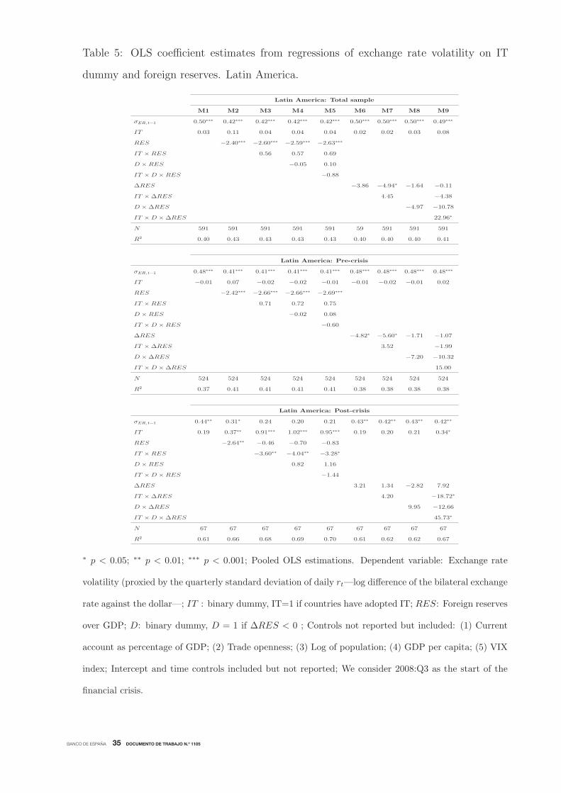
Finally, we also perform the same analysis by region, namely Latin America, Emerging
Asia and Eastern Europe. Tables 5 to 7 report these estimates, respectively.
Regarding Latin America, the main result in Table 5 is that IT× ΔRES and IT ×D×ΔRES are significant in the post-crisis period. That is, FX interventions carried out
by IT countries during the crisis were associated with lower σER, which is again a result
favorable to the use of FX interventions during crisis times in IT countries. On the other
hand, the positive link between IT and σER is identified only in the post-crisis period.
One possible interpretation might be that before the crisis σER has extreme values in
some non-IT and IT countries—before IT adoption—corresponding to different domestic
crisis episodes (for instance, Argentine, Mexico or Brazil). Finally, in Latin America
the negative relation between RES and σER is stronger in IT countries, but only in the
pre-crisis period, when a considerable amount of reserves was accumulated.
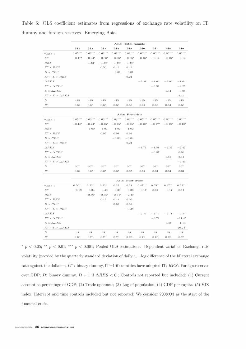
According to the estimates for Emerging Asia in Table 6, IT loses its significance in
the post-crisis period. Besides, RES is only significant in the post-crisis period and its
coefficient is higher than for the whole country sample and ΔRES plays no role neither
for IT nor non-IT countries. Finally, regarding Eastern Europe, the positive link between
IT and σER is only identified in the pre-crisis period, as reported in Table 7. However, we
do not find any significant relation between RES and the exchange rate volatility and, as
in Emerging Asia, ΔRES is not significant in any specification, as far as these estimates
seem to be dominated by the dynamics of σERt−1. All in all, the full sample results for the
post-crisis period regarding ΔRES reported in Table 4 seem to be dominated by certain
counties from our Latin American sample.

BANCO DE ESPAÑA 24 DOCUMENTO DE TRABAJO N.º 1105
6 Conclusions
In this paper we have analyzed empirically the link between exchange rate volatility,
IT and FX interventions. As far as in practice most central banks with IT have tried
to conduct monetary policy with some form of price stabilization objective and also
manage movements in its currency (“flexible IT”), these FX interventions might have
implications for monetary policy and the use of policy rules. In this sense, “flexible IT”
imply a departure from the corner solutions derived from the “impossibility Holy Trinity”
of fixed exchange rates, independent monetary policy and perfect capital mobility and
have several broad implications for the role of the exchange rate in IT countries.
To analyze this question we estimate a panel data model for 37 IT and non-IT EMEs.
We study the impact of IT adoption and foreign reserve movements—that we roughly
interpret as FX interventions—on the exchange rate volatility. We also perform this
analysis for the period previous to the onset of the financial crisis and the subsequent
sub-sample. This exercise is useful to disentangle if IT does make a difference in terms
of the impact of FX interventions on the exchange rate volatility.
We confirm that exchange rates are more volatile under IT than under other regimes
in EMEs, which is against the results in Rose (2007). However, we also show that FX
interventions in IT countries do play a useful role in containing the exchange rate volatil-
ity, especially the negative ones (sales of foreign reserves). This outcome is particularly
significant after the onset of the recent financial crisis in Latin America. Surprisingly,
this role of negative FX interventions in the moderation of the exchange rate volatility is
not identified in non-IT countries.
All in all, we support the view that there is some scope for EMEs that have adopted IT
to interpret the implementation of their IT mechanisms with certain degree of flexibility.
Thus, “flexible IT” regimes are not only sustainable, but also FX interventions performed
under this scheme are even more effective than those of non-IT countries in mitigating
extreme volatility periods. However, there is still some room for future research to analyze
if these episodes of heavy FX interventions have not undermined the credibility of these
central banks.

BANCO DE ESPAÑA 25 DOCUMENTO DE TRABAJO N.º 1105
Appendix A: Country list
Inflation targeters Non-inflation targeters
Brazil Peru Albania Guatemala
Colombia Philippines Algeria India
Czech Republic Poland Argentina Jamaica
Chile Romania Cambodia Malaysia
Ghana Slovak Republic China Morocco
Hungary South Africa Costa Rica Russia
Indonesia South Korea Croatia Singapore
Israel Thailand Dominican Republic Ukraine
Mexico Turkey Egypt Uruguay
Vietnam
Appendix B: Definition of variables and data sources
• IT: Dummy variable that is one if the country had a formal IT in that quarter.
Source: IMF (2005) and Little and Romano (2009).
• Reserves, RESit: Foreign exchange reserves over nominal GDP in US dollars.
Source: International Financial Statistics (IMF).
• Openness: Exports plus imports as a percentage of GDP. Source: International
Financial Statistics (IMF), Datastream and national sources.
• Current account: Current account as a percentage of GDP. Source: International
Financial Statistics (IMF), Datastream and national sources.
• Population: Logarithm of population (thousand persons). Source: World Economic
Outlook (IMF).
• GDP per capita: Gross domestic product based on purchasing-power-parity (PPP)
per capita. Source: World Economic Outlook (IMF).
• VIX: Implicit volatility of the S&P 500 index. Source: Datastream.

BANCO DE ESPAÑA 26 DOCUMENTO DE TRABAJO N.º 1105
References
[1] AIZENMAN, J., M. HUTCHISON and I. NOY (2008). Inflation targeting and real
exchange rates in emerging markets, NBER Working Paper No. 14561.
[2] ARELLANO, M., and S. R. BOND (1991). “Some tests of specification for panel
data: Monte Carlo evidence and an application to employment equations”, Review
of Economic Studies. 58, pp. 277-298.
[3] BALL, L., and N. SHERIDAN (2005). “Does Inflation Targeting Matter?”, in B.
Bernanke and M. Woodford (eds.), The Inflation Targeting Debate, The University
of Chicago Press, Chicago, pp. 249-276.
[4] BERNANKE, B., T. LAUBACH, A. POSEN and F. MISHKIN (1999). Inflation
targeting: Lessons from the international experience. Princeton, NJ: Princeton Uni-
versity Press.
[5] BRITO, R., and B. BYSTEDT (2010). “Inflation targeting in emerging economies:
panel evidence”, Journal of Development Economics, 91, pp. 198-210.
[6] CALVO, G., and C. REINHART (2002). “Fear of floating”, Quarterly Journal of
Economics, 117, pp. 379-408.
[7] CARRANZA, L., J. E. GALDÓN-SÁNCHEZ and J. GÓMEZ-BISCARRI (2009).
“Exchange rate and inflation dynamics in dollarized economies”, Journal of Devel-
opment Economics, 89, pp. 98-108.
[8] DE CARVALHO, I. (2010. Inflation targeting and the crisis: An empirical assess-
ment, IMF Working Paper 10/45.
[9] CAVOLI, T. (2008). “The exchange rate and optimal monetary policy rules in open
and developing economies: some simple analytics”, Economic Modelling, 25, pp.
1011-1021.
[10] – (2009). “Is fear of floating justified? The East Asia experience”, Journal of Policy
Modeling, 31, pp. 1-16.
BANCO DE ESPAÑA 27 DOCUMENTO DE TRABAJO N.º 1105
[11] CHANG, R. (2008). Inflation targeting, reserves accumulation, and exchange rate
management in Latin America, Borradores de Economía 487, Banco de la República
de Colombia.
[12] CORDERO, J. (2009). “Inflation targeting and the real exchange in a small economy:
A structuralist approach”, in G. Epstein and E. Yeldan (eds.), Beyond Inflation
Targeting, pp. 44-67.
[13] DOMAÇ, I., and A. MENDOZA (2004). Is there room for foreign exchange inter-
ventions under an inflation targeting framework? Evidence from Mexico and Turkey,
World Bank Policy Research Working Paper 3288.
[14] DOMÍNGUEZ, K. M. (1998). “Central bank intervention and exchange rate volatil-
ity”, Journal of International Money and Finance, 17, pp. 161-190.
[15] EDISON, H., P. CASHIN and H. LIANG (2006). “Foreign exchange intervention
and the Australian dollar: has it mattered?”, International Journal of Finance and
Economics, 11, pp. 155-171.
[16] EDWARDS, S. (2007). “The relationship between exchange rates and inflation tar-
geting revisited”, in F. Mishkin and K. Schmidt- Hebbel, K. (eds.), Monetary Policy
under Inflation Targeting, Banco Central de Chile, Santiago, pp. 373-413.
[17] GERŠL, A., and T. HOLUB (2006). “Foreign exchange interventions under inflation
targeting: The Czech experience”, Contemporary Economic Policy, 24, pp. 475-491.
[18] GONÇALVES, C. E., and A. CARVALHO (2008). “Who chooses to inflation tar-
get?”, Economics Letters, 99, pp. 410-413.
[19] GONÇALVES, C. E, and J. SALLES (2008). “Inflation targeting in emerging
economies: What do the data say?”, Journal of Development Economics, 85, pp.
312-318.
[20] DE GREGORIO, J., A.TOKMAN and R. VALDÉS (2005). Flexible exchange rate
with inflation targeting in Chile: Experience and issues, Inter-American Development
Bank, Working Paper No. 540.

BANCO DE ESPAÑA 28 DOCUMENTO DE TRABAJO N.º 1105
[21] GUIMARÃES, R., and C. KARACADAG (2004). The empirics of foreign exchange
intervention in emerging market countries: The cases of Mexico and Turkey, IMF
Working Paper 04/123.
[22] HABERMEIER, K., I. ÖTKER, L. JÁCOME, A. GIUSTINIANI, K. ISHI, D.
VÁVRA, T. KISINGAY and F. VÁZQUEZ (2009). Inflation pressures and monetary
policy options in emerging and developing countries - A cross regional perspective,
IMF Working Paper 06/278.
[23] HARVEY, A., E. RUIZ and N. SHEPHARD (1994). “Multivariate stochastic vari-
ance models”, The Review of Economic Studies, 61, pp. 247-264.
[24] HAUSMAN, J. (1983). “Specification and estimation of simultaneous equation mod-
els”, in Z. Griliches and M. D. Intrillgator (eds.), Handbook of Econometrics, Vol. I.
North-Holland, Amsterdam.
[25] ILZETZKI, E., C. REINHART and K. ROGOFF (2008). “Exchange rate arrange-
ments into the 21st Century: Will the anchor currency hold?”, Quarterly Journal of
Economics, pp. 119, 1-48. (Updated database).
[26] INTERNATIONAL MONETARY FUND (IMF) (2005). “Does inflation targeting
work in emerging markets?”, in World Economic Outlook, September, pp. 161-186.
[27] – (2007). Regional Economic Outlook, Asia and Pacific, October.
[28] KAMIL, H. (2008). Is central bank intervention effective under inflation targeting
regimes? The case of Colombia, IMF Working Paper 08/88.
[29] KIM, S., and J. SHEEN (2002). “The determinants of foreign exchange intervention
by central banks: evidence from Australia”, Journal of International money and
Finance, 21, pp. 619-649.
[30] KIRNASOVA, T., C. LEITH and S. WREN-LEWIS (2006). “Should central banks
target consumer prices or the exchange rate?”, The Economic Journal, 116, pp.
208-231.
BANCO DE ESPAÑA 29 DOCUMENTO DE TRABAJO N.º 1105
[31] LEVY-YEYATI, E., and F. STURZENEGGER (2007). Fear of Appreciation, KSG
Working Paper 07-047, Harvard University.
[32] LIN, S., and H. YE (2009). “Does inflation targeting make a difference in developing
countries?”, Journal of Development Economics, 89, pp. 118-123.
[33] LITTLE, J. S., and T. F. ROMANO (2009). Inflation targeting - Central bank prac-
tice overseas, Public Policy Briefs No. 08-1, Federal Reserve Bank of Boston.
[34] MIHOV. I., and A. ROSE (2008). “Is old money better than new? Duration and
monetary regimes”, Economics: The Open-Access, Open-Assessment E-Journal, 2,
2008-13.
[35] MINELLA, A., P. SPRINGER DE FREITAS, I. GOLDFAJN and M. K. MUINHOS
(2003). “Inflation targeting in Brazil: Constructing credibility under exchange rate
volatility”, Journal of International Money and Finance, 22, pp. 1015-1040.
[36] MISHKIN, F., and M. SAVASTANO (2001). “Monetary policy strategies for Latin
America”, Journal of Development Economics, 66, pp. 415-444.
[37] MISHKIN, F., and K. SCHMIDT-HEBBEL (2007). “Does inflation targeting make
a difference?”, in F. Mishkin and K. Schmidt- Hebbel (eds.), Monetary Policy under
Inflation Targeting, Banco Central de Chile, Santiago, pp. 291-372.
[38] OBSTFELD, M., J. C. SHAMBAUGH and A. M. TAYLOR (2005). “The trilemma
in history: Tradeoffs among exchange rates, monetary policies, and capital mobility”,
The Review of Economics and Statistics, 87, pp. 423-438.
[39] PARRADO, E. (2004). Inflation targeting and exchange rules in an open economy,
IMF Working Paper 04/21.
[40] ROGER, S., J. RESTREPO and C. GARCÍA (2009). Hybrid inflation targeting
regimes, IMF Working Paper 09/234.
[41] ROSE, A. (2007). “A stable international monetary system emerges: Inflation tar-
geting is Bretton Woods, reversed”, Journal of International Money and Finance,
26, pp. 663-681.

BANCO DE ESPAÑA 30 DOCUMENTO DE TRABAJO N.º 1105
[42] STONE, M., S. ROGER, S. SHIMIZU, A. NORDSTROM, T. KISINBAY and
J. RESTREPO (2009). The role of exchange rate in inflation-targeting emerging
economies, IMF Ocassional Paper No. 267.
[43] SVENSSON, L. (2010). Inflation targeting, NBER Working Paper 16654.
[44] TAYLOR, J. (2000). “Low inflation, pass-through and the pricing power of firms”,
European Economic Review, 7, pp. 1389-1408.
[45] WU, D. (1973).”Alternative tests of independence between stochastic regressors and
disturbances”, Econometrica, 41, pp. 733-750.
[46] YILMAZKUDAY, H. (2007). “Inflation targeting supported by managed exchange
rate”, Applied Economics, 39, pp. 2011-2026.

BANCO DE ESPAÑA 31 DOCUMENTO DE TRABAJO N.º 1105
Figure 1: Six-quarter rolling window estimates. Total effect of negative FX interventions
(D = 1) on the exchange rate volatility in non-IT (left), and IT countries (right).
−25
−20
−15
−10
−50
Non−I
T co
untri
es
2000q1 2002q3 2005q1 2007q3 2010q1
−10
010
20IT
cou
ntrie
s
2000q1 2002q3 2005q1 2007q3 2010q1
Figure 2: Six-quarter rolling window estimates. Total effect of positive FX interventions
(D = 0) on the exchange rate volatility in non-IT (left), and IT countries (right).
−10
010
2030
Non−I
T co
untri
es
2000q1 2002q3 2005q1 2007q3 2010q1
−50
510
IT c
ount
ries
2000q1 2002q3 2005q1 2007q3 2010q1
BANCO DE ESPAÑA 32 DOCUMENTO DE TRABAJO N.º 1105
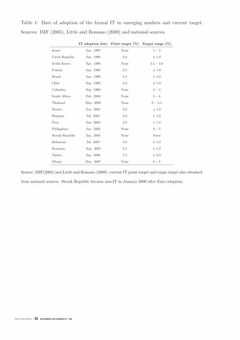
Table 1: Date of adoption of the formal IT in emerging markets and current target.
Sources: IMF (2005), Little and Romano (2009) and national sources.
IT adoption date Point target (%) Target range (%)
Israel Jun. 1997 None 1 − 3
Czech Republic Jan. 1998 3.0 ± 1.0
South Korea Apr. 1998 None 3.5 − 4.0
Poland Jan. 1999 2.5 ± 1.0
Brazil Jun. 1999 4.5 ± 2.0
Chile Sep. 1999 3.0 ± 1.0
Colombia Sep. 1999 None 2 − 4
South Africa Feb. 2000 None 3 − 6
Thailand May. 2000 None 0 − 3.5
Mexico Jan. 2001 3.0 ± 1.0
Hungary Jul. 2001 3.0 ± 1.0
Peru Jan. 2002 2.0 ± 1.0
Philippines Jan. 2002 None 4 − 5
Slovak Republic Jan. 2005 None None
Indonesia Jul. 2005 5.0 ± 1.0
Romania Aug. 2005 3.5 ± 1.0
Turkey Jan. 2006 7.5 ± 2.0
Ghana May. 2007 None 6 − 8
Source: IMF(2005) and Little and Romano (2009); current IT point target and range target also obtained
from national sources. Slovak Republic became non-IT in January 2009 after Euro adoption.

BANCO DE ESPAÑA 33 DOCUMENTO DE TRABAJO N.º 1105
Table 2: Summary statistics of σER, RES, ΔRES and D × ΔRES for a sample of
37 countries (quarterly data, based on nominal exchange rates against the dollar). We
consider 2008:Q3 as the date of the beginning of the crisis.
Mean CV Max Min
IT Non-IT IT Non-IT IT Non-IT IT Non-IT
σER Full sample 0.643 0.507 0.676 1.289 4.507 8.637 0.041 0.000
Pre crisis 0.565 0.501 0.561 1.331 2.818 8.637 0.041 0.000
After crisis 0.971 0.575 0.676 0.861 4.507 4.251 0.141 0.000
RES Full sample 0.167 0.186 0.444 0.984 0.505 1.026 0.036 0.006
Pre crisis 0.164 0.177 0.420 0.987 0.415 1.026 0.036 0.006
After crisis 0.187 0.285 0.502 0.830 0.505 1.018 0.082 0.041
ΔRES Full sample 0.002 0.002 7.311 6.916 0.086 0.080 −0.043 −0.101
Pre crisis 0.001 0.003 11.521 5.312 0.086 0.080 −0.043 −0.085
After crisis 0.005 −0.003 3.550 −7.871 0.061 0.069 −0.028 −0.101
D × ΔRES Full sample −0.003 −0.004 −1.833 −2.162 0.000 0.000 −0.043 −0.101
Pre crisis −0.003 −0.003 −1.848 −2.148 0.000 0.000 −0.043 −0.085
After crisis −0.004 −0.010 −1.743 −1.639 0.000 0.000 −0.028 −0.101
Summary statistics of the exchange rate volatility based on nominal exchange rates against the dollar
(σER), the stock of foreign reserves (RES); FX interventions (ΔRES) and negative FX interventions
(D×ΔRES). CV: coefficient of variation (standard deviation / mean); Max: Maximum; Min: Minimum.
Table 3: Correlation matrix
σER IT RES ΔRES D × ΔRES Current account Openness Population GDP per capita VIX
σER 1
IT 0.10∗ 1
RES −0.14∗ −0.05∗ 1
ΔRES 0.00 −0.01 0.12∗ 1
D × ΔRES −0.05∗ 0.05∗ −0.18∗ 0.74∗ 1
Current account −0.06∗ −0.08∗ 0.65∗ 0.15∗ −0.05∗ 1
Openness 0.03 0.01 0.11∗ −0.04 −0.02 −0.10∗ 1
Population −0.07∗ 0.08∗ −0.14∗ 0.04 0.09∗ 0.12∗ −0.20∗ 1
GDP per capita 0.05∗ 0.36∗ 0.39∗ −0.01 −0.10∗ 0.24∗ 0.16∗ −0.38∗ 1
VIX 0.25∗ 0.05∗ 0.02 −0.03 −0.09∗ −0.02 −0.02 0.01 0.05∗ 1
∗ significant pairwise correlation at 5%.

BANCO DE ESPAÑA 34 DOCUMENTO DE TRABAJO N.º 1105
Table 4: OLS coefficient estimates from regressions of exchange rate volatility on IT
dummy and foreign reserves.
Total sample
M1 M2 M3 M4 M5 M6 M7 M8 M9
σER, t−1 0.53∗∗∗ 0.52∗∗∗ 0.51∗∗∗ 0.51∗∗∗ 0.51∗∗∗ 0.53∗∗∗ 0.53∗∗∗ 0.53∗∗∗ 0.53∗∗∗
IT 0.07∗∗ 0.05 0.15∗∗ 0.15∗∗ 0.15∗∗ 0.07∗∗ 0.07∗∗ 0.07∗∗ 0.10∗∗∗
RES −0.45∗∗∗ −0.40∗∗∗ −0.39∗∗ −0.39∗∗
IT × RES −0.56∗∗ −0.56∗∗ −0.54∗∗
D × RES −0.01 0.01
IT × D × RES −0.31∗
ΔRES −0.57 −0.45 0.70 1.70
IT × ΔRES −0.58 −3.32
D × ΔRES −3.03 −4.85
IT × D × ΔRES 9.30∗∗
N 2048 2039 2039 2039 2039 2036 2036 2036 2036
R2 0.39 0.40 0.40 0.40 0.40 0.39 0.39 0.39 0.39
Pre-crisis
σER, t−1 0.52∗∗∗ 0.51∗∗∗ 0.51∗∗∗ 0.51∗∗∗ 0.51∗∗∗ 0.53∗∗∗ 0.53∗∗∗ 0.53∗∗∗ 0.52∗∗∗
IT 0.06∗ 0.04 0.12∗ 0.12∗ 0.13∗ 0.06∗ 0.06∗ 0.07∗ 0.09∗∗
RES −0.48∗∗∗ −0.44∗∗ −0.44∗∗ −0.44∗∗
IT × RES −0.48∗ −0.49∗ −0.46∗
D × RES 0.01 0.02
IT × D × RES −0.35∗∗
ΔRES −0.68 −0.82 1.11 1.61
IT × ΔRES 0.80 −1.96
D × ΔRES −4.49 −6.05
IT × D × ΔRES 8.99∗∗
N 1819 1810 1810 1810 1810 1807 1807 1807 1807
R2 0.35 0.36 0.36 0.36 0.36 0.35 0.35 0.36 0.36
Post-crisis
σER, t−1 0.51∗∗∗ 0.51∗∗∗ 0.48∗∗∗ 0.48∗∗∗ 0.48∗∗∗ 0.51∗∗∗ 0.52∗∗∗ 0.52∗∗∗ 0.50∗∗∗
IT 0.11 0.10 0.31∗∗ 0.32∗∗ 0.32∗∗ 0.13∗ 0.14∗ 0.12∗ 0.20∗∗
RES −0.15 −0.02 −0.05 −0.04
IT × RES −0.98∗∗ −0.97∗∗ −0.95∗
D × RES 0.08 0.10
IT × D × RES −0.28
ΔRES −1.53 −0.38 −2.50 2.19
IT × ΔRES −3.49 −7.41∗
D × ΔRES 1.95 −4.05
IT × D × ΔRES 15.82∗
N 229 229 229 229 229 229 229 229 229
R2 0.57 0.57 0.58 0.58 0.58 0.57 0.57 0.57 0.58
∗ p < 0.05; ∗∗ p < 0.01; ∗∗∗ p < 0.001; Pooled OLS estimations. Dependent variable: Exchange rate
volatility (proxied by the quarterly standard deviation of daily rt—log difference of the bilateral exchange
rate against the dollar—; IT : binary dummy, IT=1 if countries have adopted IT; RES: Foreign reserves
over GDP; D: binary dummy, D = 1 if ΔRES < 0 ; Controls not reported but included: (1) Current
account as percentage of GDP; (2) Trade openness; (3) Log of population; (4) GDP per capita; (5) VIX
index; Intercept and time controls included but not reported; We consider 2008:Q3 as the start of the
financial crisis.
BANCO DE ESPAÑA 35 DOCUMENTO DE TRABAJO N.º 1105
Table 5: OLS coefficient estimates from regressions of exchange rate volatility on IT
dummy and foreign reserves. Latin America.
Latin America: Total sample
M1 M2 M3 M4 M5 M6 M7 M8 M9
σER, t−1 0.50∗∗∗ 0.42∗∗∗ 0.42∗∗∗ 0.42∗∗∗ 0.42∗∗∗ 0.50∗∗∗ 0.50∗∗∗ 0.50∗∗∗ 0.49∗∗∗
IT 0.03 0.11 0.04 0.04 0.04 0.02 0.02 0.03 0.08
RES −2.40∗∗∗ −2.60∗∗∗ −2.59∗∗∗ −2.63∗∗∗
IT × RES 0.56 0.57 0.69
D × RES −0.05 0.10
IT × D × RES −0.88
ΔRES −3.86 −4.94∗ −1.64 −0.11
IT × ΔRES 4.45 −4.38
D × ΔRES −4.97 −10.78
IT × D × ΔRES 22.96∗
N 591 591 591 591 591 59 591 591 591
R2 0.40 0.43 0.43 0.43 0.43 0.40 0.40 0.40 0.41
Latin America: Pre-crisis
σER, t−1 0.48∗∗∗ 0.41∗∗∗ 0.41∗∗∗ 0.41∗∗∗ 0.41∗∗∗ 0.48∗∗∗ 0.48∗∗∗ 0.48∗∗∗ 0.48∗∗∗
IT −0.01 0.07 −0.02 −0.02 −0.01 −0.01 −0.02 −0.01 0.02
RES −2.42∗∗∗ −2.66∗∗∗ −2.66∗∗∗ −2.69∗∗∗
IT × RES 0.71 0.72 0.75
D × RES −0.02 0.08
IT × D × RES −0.60
ΔRES −4.82∗ −5.60∗ −1.71 −1.07
IT × ΔRES 3.52 −1.99
D × ΔRES −7.20 −10.32
IT × D × ΔRES 15.00
N 524 524 524 524 524 524 524 524 524
R2 0.37 0.41 0.41 0.41 0.41 0.38 0.38 0.38 0.38
Latin America: Post-crisis
σER, t−1 0.44∗∗ 0.31∗ 0.24 0.20 0.21 0.43∗∗ 0.42∗∗ 0.43∗∗ 0.42∗∗
IT 0.19 0.37∗∗ 0.91∗∗∗ 1.02∗∗∗ 0.95∗∗∗ 0.19 0.20 0.21 0.34∗
RES −2.64∗∗ −0.46 −0.70 −0.83
IT × RES −3.60∗∗ −4.04∗∗ −3.28∗
D × RES 0.82 1.16
IT × D × RES −1.44
ΔRES 3.21 1.34 −2.82 7.92
IT × ΔRES 4.20 −18.72∗
D × ΔRES 9.95 −12.66
IT × D × ΔRES 45.73∗
N 67 67 67 67 67 67 67 67 67
R2 0.61 0.66 0.68 0.69 0.70 0.61 0.62 0.62 0.67
∗ p < 0.05; ∗∗ p < 0.01; ∗∗∗ p < 0.001; Pooled OLS estimations. Dependent variable: Exchange rate
volatility (proxied by the quarterly standard deviation of daily rt—log difference of the bilateral exchange
rate against the dollar—; IT : binary dummy, IT=1 if countries have adopted IT; RES: Foreign reserves
over GDP; D: binary dummy, D = 1 if ΔRES < 0 ; Controls not reported but included: (1) Current
account as percentage of GDP; (2) Trade openness; (3) Log of population; (4) GDP per capita; (5) VIX
index; Intercept and time controls included but not reported; We consider 2008:Q3 as the start of the
financial crisis.
BANCO DE ESPAÑA 36 DOCUMENTO DE TRABAJO N.º 1105
Table 6: OLS coefficient estimates from regressions of exchange rate volatility on IT
dummy and foreign reserves. Emerging Asia.
Asia: Total sample
M1 M2 M3 M4 M5 M6 M7 M8 M9
σER, t−1 0.65∗∗∗ 0.62∗∗∗ 0.62∗∗∗ 0.62∗∗∗ 0.62∗∗∗ 0.66∗∗∗ 0.66∗∗∗ 0.66∗∗∗ 0.66∗∗∗
IT −0.17∗ −0.24∗ −0.36∗ −0.36∗ −0.36∗ −0.16∗ −0.14 −0.16∗ −0.14
RES −1.12∗ −1.18∗ −1.18∗ −1.18∗
IT × RES 0.50 0.49 0.49
D × RES −0.01 −0.01
IT × D × RES 0.21
ΔRES −2.38 −1.66 −2.96 −1.64
IT × ΔRES −3.91 −4.25
D × ΔRES 1.44 −0.05
IT × D × ΔRES 2.15
N 415 415 415 415 415 415 415 415 415
R2 0.64 0.65 0.65 0.65 0.65 0.64 0.65 0.64 0.65
Asia: Pre-crisis
σER, t−1 0.65∗∗∗ 0.63∗∗∗ 0.63∗∗∗ 0.63∗∗∗ 0.63∗∗∗ 0.65∗∗∗ 0.65∗∗∗ 0.66∗∗∗ 0.66∗∗∗
IT −0.18∗ −0.24∗ −0.45∗ −0.45∗ −0.45∗ −0.18∗ −0.17∗ −0.18∗ −0.18∗
RES −1.00 −1.01 −1.02 −1.02
IT × RES 0.95 0.94 0.94
D × RES −0.03 −0.04
IT × D × RES 0.21
ΔRES −1.71 −1.58 −2.37 −2.47
IT × ΔRES −0.87 0.09
D × ΔRES 1.61 2.11
IT × D × ΔRES −3.45
N 367 367 367 367 367 367 367 367 367
R2 0.64 0.65 0.65 0.65 0.65 0.64 0.64 0.64 0.64
Asia: Post-crisis
σER, t−1 0.50∗∗ 0.22∗ 0.22∗ 0.22 0.21 0.47∗∗∗ 0.55∗∗ 0.47∗∗ 0.52∗∗
IT −0.19 −0.34 −0.40 −0.39 −0.36 −0.17 0.01 −0.17 0.11
RES −2.46∗ −2.55∗ −2.54∗ −2.49
IT × RES 0.12 0.11 0.06
D × RES 0.02 0.02
IT × D × RES −0.38
ΔRES −6.37 −3.72 −6.78 −2.34
IT × ΔRES −8.71 −11.45
D × ΔRES 1.03 −1.13
IT × D × ΔRES 26.23
N 48 48 48 48 48 48 48 48 48
R2 0.66 0.73 0.73 0.73 0.73 0.70 0.73 0.70 0.75
∗ p < 0.05; ∗∗ p < 0.01; ∗∗∗ p < 0.001; Pooled OLS estimations. Dependent variable: Exchange rate
volatility (proxied by the quarterly standard deviation of daily rt—log difference of the bilateral exchange
rate against the dollar—; IT : binary dummy, IT=1 if countries have adopted IT; RES: Foreign reserves
over GDP; D: binary dummy, D = 1 if ΔRES < 0 ; Controls not reported but included: (1) Current
account as percentage of GDP; (2) Trade openness; (3) Log of population; (4) GDP per capita; (5) VIX
index; Intercept and time controls included but not reported; We consider 2008:Q3 as the start of the
financial crisis.

BANCO DE ESPAÑA 37 DOCUMENTO DE TRABAJO N.º 1105
Table 7: OLS coefficient estimates from regressions of exchange rate volatility on IT
dummy and foreign reserves. Eastern Europe.
Eastern Europe: Total sample
M1 M2 M3 M4 M5 M6 M7 M8 M9
σER, t−1 0.36∗∗∗ 0.36∗∗∗ 0.36∗∗∗ 0.36∗∗∗ 0.36∗∗∗ 0.37∗∗∗ 0.37∗∗∗ 0.37∗∗∗ 0.37∗∗∗
IT 0.13∗∗ 0.11∗ 0.10 0.11 0.12 0.12∗∗ 0.12∗∗ 0.13∗∗ 0.12∗∗
RES −0.64 −0.65 −0.70 −0.70
IT × RES 0.04 −0.04 −0.06
D × RES 0.23 0.27
IT × D × RES −0.24
ΔRES −1.46 −2.04 −1.11 −2.04
IT × ΔRES 1.73 2.00
D × ΔRES −0.87 −0.01
IT × D × ΔRES −1.41
N 604 604 604 604 604 604 604 604 604
R2 0.36 0.36 0.36 0.36 0.36 0.36 0.36 0.36 0.36
Eastern Europe: Pre-crisis
σER, t−1 0.36∗∗∗ 0.35∗∗∗ 0.35∗∗∗ 0.35∗∗∗ 0.35∗∗∗ 0.36∗∗∗ 0.36∗∗∗ 0.36∗∗∗ 0.36∗∗∗
IT 0.12∗∗ 0.09 0.09 0.11 0.13 0.11∗ 0.11∗ 0.11∗∗ 0.11∗
RES −0.82 −0.82 −0.87 −0.88
IT × RES 0.04 −0.11 −0.16
D × RES 0.27 0.32
IT × D × RES −0.33
ΔRES −1.92 −2.91 −1.17 −2.03
IT × ΔRES 3.45 2.92
D × ΔRES −2.01 −2.31
IT × D × ΔRES 1.90
N 532 532 532 532 532 532 532 532 532
R2 0.26 0.26 0.26 0.27 0.27 0.26 0.26 0.26 0.26
Eastern Europe: Post-crisis
σER, t−1 0.35∗∗∗ 0.34∗∗∗ 0.31∗ 0.31∗ 0.31∗ 0.35∗∗∗ 0.36∗∗∗ 0.35∗∗ 0.35∗∗
IT 0.19 0.16 −0.80 −0.91 −0.94 0.19 0.19 0.17 0.14
RES −0.58 −4.04 −4.30 −4.31
IT × RES 4.23 4.66 4.66
D × RES −0.32 −0.45
IT × D × RES 0.66
ΔRES 0.11 1.68 −1.36 −0.71
IT × ΔRES −3.30 −0.59
D × ΔRES 3.31 3.89
IT × D × ΔRES −9.31
N 72 72 72 72 72 72 72 72 72
R2 0.53 0.53 0.54 0.54 0.54 0.53 0.53 0.53 0.53
∗ p < 0.05; ∗∗ p < 0.01; ∗∗∗ p < 0.001; Pooled OLS estimations. Dependent variable: Exchange rate
volatility (proxied by the quarterly standard deviation of daily rt—log difference of the bilateral exchange
rate against the dollar—; IT : binary dummy, IT=1 if countries have adopted IT; RES: Foreign reserves
over GDP; D: binary dummy, D = 1 if ΔRES < 0 ; Controls not reported but included: (1) Current
account as percentage of GDP; (2) Trade openness; (3) Log of population; (4) GDP per capita; (5) VIX
index; Intercept and time controls included but not reported; We consider 2008:Q3 as the start of the
financial crisis.

BANCO DE ESPAÑA PUBLICATIONS
WORKING PAPERS1
0922
GALO NUÑO: Technology, convergence and business cycles.
0923 FRANCISCO DE CASTRO AND JOSÉ LUIS FERNÁNDEZ: The relationship between public and private saving in
Spain: does Ricardian equivalence hold?
0924 GONZALO FERNÁNDEZ-DE-CÓRDOBA, JAVIER J. PÉREZ AND JOSÉ L. TORRES: Public and private sector wages
interactions in a general equilibrium model.
0925 ÁNGEL ESTRADA AND JOSÉ MANUEL MONTERO: R&D investment and endogenous growth: a SVAR approach.
0926 JUANA ALEDO, FERNANDO GARCÍA-MARTÍNEZ AND JUAN M. MARÍN DIAZARAQUE: Firm-specific factors
influencing the selection of accounting options provided by the IFRS: Empirical evidence from Spanish market.
0927 JAVIER ANDRÉS, SAMUEL HURTADO, EVA ORTEGA AND CARLOS THOMAS: Spain in the euro: a general
equilibrium analysis.
0928 MAX GILLMAN AND ANTON NAKOV: Monetary effects on nominal oil prices.
0929
0930
0931
JAVIER MENCÍA AND ENRIQUE SENTANA: Distributional tests in multivariate dynamic models with Normal and
Student t innovations.
JOAN PAREDES, PABLO BURRIEL, FRANCISCO DE CASTRO, DANIEL GARROTE, ESTHER GORDO AND JAVIER
J. PÉREZ: Fiscal policy shocks in the euro area and the US: an empirical assessment.
TERESA LEAL, DIEGO J. PEDREGAL AND JAVIER J. PÉREZ: Short-term monitoring of the Spanish Government
balance with mixed-frequencies models.
0932 ANTON NAKOV AND GALO NUÑO: Oilgopoly: a general equilibrium model of the oil-macroeconomy nexus.
0933 TERESA LEAL AND JAVIER J. PÉREZ: Análisis de las desviaciones presupuestarias aplicado al caso del presupuesto
del Estado.
0934 JAVIER J. PÉREZ AND A. JESÚS SÁNCHEZ: Is there a signalling role for public wages? Evidence for the euro area
based on macro data.
0935
1001
JOAN PAREDES, DIEGO J. PEDREGAL AND JAVIER J. PÉREZ: A quarterly fiscal database for the euro area based
on intra-annual fiscal information.
JAVIER ANDRÉS, ÓSCAR ARCE AND CARLOS THOMAS: Banking competition, collateral constraints and optimal
monetary policy.
1002 CRISTINA BARCELÓ AND ERNESTO VILLANUEVA: The response of household wealth to the risk of losing the job:
evidence from differences in firing costs.
1003
1004
ALEXANDER KARAIVANOV, SONIA RUANO, JESÚS SAURINA AND ROBERT TOWNSEND: No bank, one bank,
several banks: does it matter for investment?
GABRIEL PEREZ-QUIROS AND HUGO RODRÍGUEZ MENDIZÁBAL: Asymmetric standing facilities: an unexploited
monetary policy tool.
1005
1006
1007
1008
GABRIEL JIMÉNEZ, JOSE A. LOPEZ AND JESÚS SAURINA: How does competition impact bank
risk-taking?
GIUSEPPE BERTOLA, AURELIJUS DABUSINSKAS, MARCO HOEBERICHTS, MARIO IZQUIERDO, CLAUDIA
KWAPIL, JEREMI MONTORNÈS AND DANIEL RADOWSKI: Price, wage and employment response to shocks:
evidence from the WDN Survey.
JAVIER MENCÍA: Testing non-linear dependence in the Hedge Fund industry.
ALFREDO MARTÍN-OLIVER: From proximity to distant banking: Spanish banks in the EMU.
1009 GALO NUÑO: Optimal research and development expenditure: a general equilibrium approach.
1010
1011
1012
1013
1014
1015
LUIS J. ÁLVAREZ AND PABLO BURRIEL: Is a Calvo price setting model consistent with micro price data?
JENS HAGENDORFF, IGNACIO HERNANDO, MARÍA J. NIETO AND LARRY D. WALL: What do premiums paid for
bank M&As reflect? The case of the European Union.
DAVID DE ANTONIO LIEDO: General equilibrium restrictions for dynamic factor models.
JAMES COSTAIN, JUAN F. JIMENO AND CARLOS THOMAS: Employment fluctuations in a dual labor market.
LUIS M. VICEIRA AND RICARDO GIMENO: The euro as a reserve currency for global investors.
PALOMA LÓPEZ-GARCÍA AND JOSÉ MANUEL MONTERO: Understanding the Spanish business innovation gap:
The role of spillovers and firms' absorptive capacity.
1. Previously published Working Papers are listed in the Banco de España publications catalogue.
1016
1017
1018
1019
1020
1021
1022
1023
1024
1025
1026
1027
1028
1029
1030
1031
1032
1033
1034
1035
1036
1037
1038
1039
1101
1102
1103
1104
1105
AITOR LACUESTA AND SERGIO PUENTE: El efecto del ciclo económico en las entradas y salidas de inmigrantes
en España.
REBEKKA CHRISTOPOULOU, JUAN F. JIMENO AND ANA LAMO: Changes in the wage structure in EU countries.
THOMAS BREUER, MARTIN JANDAČKA, JAVIER MENCÍA AND MARTIN SUMMER: A systematic approach to
multi-period stress testing of portfolio credit risk.
LUIS J. ÁLVAREZ AND PABLO BURRIEL: Micro-based estimates of heterogeneous pricing rules: The United States
vs. the euro area.
ALFREDO MARTÍN-OLIVER AND VICENTE SALAS-FUMÁS: I.T. investment and intangibles: Evidence from banks.
LUISA LAMBERTINI, CATERINA MENDICINO AND MARIA TERESA PUNZI: Expectations-driven cycles
in the housing market.
JULIÁN MESSINA, PHILIP DU CAJU, CLÁUDIA FILIPA DUARTE, NIELS LYNGGÅRD HANSEN AND MARIO
IZQUIERDO: The incidence of nominal and real wage rigidity: an individual-based sectoral approach.
ALESSIO MORO: Development, growth and volatility.
LUIS J. ÁLVAREZ AND ALBERTO CABRERO: Does housing really lead the business cycle?
JUAN S. MORA-SANGUINETTI: Is judicial inefficiency increasing the house property market weight in Spain?
Evidence at the local level.
MAXIMO CAMACHO, GABRIEL PEREZ-QUIROS AND PILAR PONCELA: Green shoots in the Euro area. A real
time measure.
AITOR ERCE AND JAVIER DÍAZ-CASSOU: Creditor discrimination during sovereign debt restructurings.
RAFAEL REPULLO, JESÚS SAURINA AND CARLOS TRUCHARTE: Mitigating the pro-cyclicality of Basel II.
ISABEL ARGIMÓN AND JENIFER RUIZ: The effects of national discretions on banks.
GABRIEL JIMÉNEZ, STEVEN ONGENA, JOSÉ-LUIS PEYDRÓ AND JESÚS SAURINA: Credit supply: identifying
balance-sheet channels with loan applications and granted loans.
ENRIQUE MORAL-BENITO: Determinants of economic growth: A Bayesian panel data approach.
GABE J. DE BONDT, TUOMAS A. PELTONEN AND DANIEL SANTABÁRBARA: Booms and busts in China's stock
market: Estimates based on fundamentals.
CARMEN MARTÍNEZ-CARRASCAL AND JULIAN VON LANDESBERGER: Explaining the demand for money by non-
financial corporations in the euro area: A macro and a micro view.
CARMEN MARTÍNEZ-CARRASCAL: Cash holdings, firm size and access to external finance. Evidence for
the euro area.
CÉSAR ALONSO-BORREGO: Firm behavior, market deregulation and productivity in Spain.
OLYMPIA BOVER: Housing purchases and the dynamics of housing wealth.
DAVID DE ANTONIO LIEDO AND ELENA FERNÁNDEZ MUÑOZ: Nowcasting Spanish GDP growth in real time: “One
and a half months earlier”.
FRANCESCA VIANI: International financial flows, real exchange rates and cross-border insurance.
FERNANDO BRONER, TATIANA DIDIER, AITOR ERCE AND SERGIO L. SCHMUKLER: Gross capital flows: dynamics
and crises.
GIACOMO MASIER AND ERNESTO VILLANUEVA: Consumption and initial mortgage conditions: evidence from
survey data.
PABLO HERNÁNDEZ DE COS AND ENRIQUE MORAL-BENITO: Endogenous fiscal consolidations.
CÉSAR CALDERÓN, ENRIQUE MORAL-BENITO AND LUIS SERVÉN: Is infrastructure capital productive? A dynamic
heterogeneous approach.
MICHAEL DANQUAH, ENRIQUE MORAL-BENITO AND BAZOUMANA OUATTARA: TFP growth and its determinants:
nonparametrics and model averaging.
JUAN CARLOS BERGANZA AND CARMEN BROTO: Flexible inflation targets, forex interventions and exchange rate
volatility in emerging countries.
Unidad de Publicaciones Alcalá 522, 28027 Madrid
Telephone +34 91 338 6363. Fax +34 91 338 6488 E-mail: [email protected]
www.bde.es


