Download - Finit Diff

SCHAUM’S OUTLINE OF
THEORY ANB PROBLEMS
OF
Calculus
FINITE ENCES and
DIFFERENCE EQUAT
w e
BY
MURRAY R. SPIEGEL, Ph.D. Professor of Mathematics
Rensselaer Polytechnic Znstitute
SCHAUM’S OUTLINE SERIES McGRAW-HILL BOOM COMPANY
New York, St. Louis, San Francisco, Dusseldorf, Johannesburg, Kuala Lumpur, London, Mexico, Montreal, New Delhi, Panama, Rio de Janeiro, Singapore, Sydney, and Toronto

Copyright @ 1971 by McGraw-Hill, Inc. All rights reserved. Printed in the United States of America. No par t of this publication may be reproduced, stored in a retrieval system, or transmitted, in any form or by any means, electronic, mechanical, photocopying, recording, or otherwise, without the pr ior written permission of the publisher.
07-060218-2
5 6 7 8 9 10 11 12 13 14 15 SH SH 8 7 6 5 4 3 2 1

In recent years there has been an increasing interest in the calculus of finite differences and difference equations. There are several reasons for this. First, the advent of high speed computers has led to a need for fundamental knowledge of this s.ubject. Second, there are numerous applications of the subject to fields ranging from engineering, physics and chemistry to actuarial science, economics, psychology, biology, probability and statistics. Third, the mathematical theory is of interest in itself especially in view of the remarkable analogy of the theory to that of differential and integral calculus and differential equations.
This book is designed to be used either as a textbook for a formal course in the calculus of finite differences and difference equations or as a comprehensive supplement to all current standard texts. It should also be of considerable value to those taking courses in which difference methods are employed or to those interested in the field fo r self-study.
Each chapter begins with a clear statement of pertinent definitions, principles and theorems, together with illustrative and other descriptive material. The solved problems serve to illustrate and amplify the theory, bring into sharp focus those fine points without which the student continually feels himself on unsafe ground, and provide the repetition of basic principles so vital to effective learning. Numerous proofs of theorems and derivations of formulas are included among the solved problems. The large number of supplementary problems with answers serves as a complete review of the material of each chapter.
Topics covered include the difference calculus, the sum calculus and difference equations [analogous to differential calculus, integral calculus and differential equations respectively] together with many applications.
Considerably more material has been included here than can be covered in most first courses. This has been done to make the book more flexible, to provide a more useful book of reference, and to stimulate further interest in the topics.
I wish to take this opportunity to thank Nicola Monti, David Beckwith and Henry Hayden for their splendid cooperation.
Rensselaer Polytechnic Institute November 1970
M. R. SPIEGEL


C O N T E N T S
Page Chapter 1 THE DIFFERENCE CALCULUS .............................. 1
Operators. Some Definitions Involving Operators. Algebra of Operators. The Difference Operator. The Translation or Shifting Operator. The Deriva- tive Operator. The Differential Operator. Relationship Between Difference, Derivative and Differential Operators. General Rules of Differentiation. De- rivatives of Special Functions. General Rules of the Difference Calculus. Fac- torial Polynomials. Stirling Numbers. Generalized Factorial Functions. Differences of Special Functions. Taylor Series. Taylor Series in Operator Form. The Gregory-Newton Formula, Leibnitz’s Rule. Other Difference Operators.
Chapter 2 APPLICATIONS OF THE DIFFERENCE CALCULUS . . . . . . . . 32 Subscript Notation. Difference Tables. Differences of Polynomials. Gregory- Newton Formula in Subscript Notation. General Term of a Sequence or Series. Interpolation and Extrapolation, Central Difference Tables. Generalized Interpolation Formulas. Zig-Zag Paths and Lozenge Diagrams. Lagrange’s Interpolation Formula. Tables with Missing Entries. Divided Differences. Newton’s Divided Difference Interpolation Formula, Inverse Interpolation. Approximate Differentiation:
Chapter 3 THE SUM CALCULUS . . . . . . . . . . . . . . . . . . . . . . . . . . . . . . . . . . . . . . . . . 79 The Integral Operator. General Rules of Integration. Integrals of Special Functions. Definite Integrals. Fundamental Theorem of Integral Calculus. Some Important Properties of Definite Integrals. Some Important Theorems of Integral Calculus. The Sum Operator, General Rules of Summation. Sum- mations of Special Functions. Definite Sums and the Fundamental Theorem of Sum Calculus. Differentiation and Integration of Sums, Theorems on Summation Using the Subscript Notation. Abel’s Transformation. Operator Methods for Summation. Summation of Series. The Gamma Function. Ber- noulli Numbers and Polynomials, Important Properties of Bernoulli Numbers and Polynomials. Euler Numbers and Polynomials. Important Properties of Euler Numbers and Polynomials.
Chapter 4 APPLICATIONS OF THE SUM CALCULUS . . . . . . . . . . . . . . . . . . 121 Some Special Methods for Exact Summation of Series. Series of Constants. Power Series. Approximate Integration. Er ror Terms in Approximate Inte- gration Formulas. Gregory’s Formula for Approximate Integration. The Euler-Maclaurin Formula, Er ror Term in Euler-Maclaurin Formula. Stirling’s Formula for n !

C O N T E N T S
Page
Chapter 5 DIFFERENCE EQUATIONS . . . . . . . . . . . . . . . . . . . . . . . . . . . . . . . . . . 150 Differential Equations. Order of a Dif- ference Equation, Solution, General Solution and Particular Solution of a Difference Equation. Differential Equations as Limits of Difference Equations. Use of the Subscript Notation. Linear Difference Equations. Homogeneous Linear Difference Equations. Homogeneous Linear Difference Equations with Constant Coefficients. Line:rly Independent Solutions. Solution of the Non- homogeneous or Complete Equation. Methods of Finding Particular Solutions. Method of Undetermined Coefficients. Special Operator Methods. Method of Variation of Parameters. Method of Reduction of Order. Method of Generating Functions. Linear Difference Equations with Variable Coefficients. Sturm- Liouville Difference Equations. Nonlinear Difference Equations. Simultaneous Difference Equations. Mixed Difference Equations. Partial Difference Equations.
Definition of a Difference Equation.
Chapter 6 APPLICATIONS OF DIFFERENCE EQUATIONS . . . . . . . . . . . . 199 Formulation of Problems Involving Difference Equations. Applications to Vibrating Systems. Applications to Electrical Networks. Applications to Beams. Applications to Collisions. Applications to Probability. The Fibonacci Numbers. Miscellaneous Applications.
Appendix A Stirling Numbers of the Firs t Kind s; . . . . . . . . . . . . . . . . . . . . . . . . . . . . . . . . . 232
Appendix B Stirling Numbers of the Second Kind ,YE.. . . . . . . . . . . . . . . . . . . . . . . . . . . . . . . . 233
Appendix c Bernoulli Numbers . . . . . . . . . . . . . . . . . . . . . . . . . . . . . . . . . . . . . . . . . . . . . . . . . . . 234
Appendix D Bernoulli Polynomials . . . . . . . . . . . . . . . . . . . . . . . . . . . . . . . . . . . . . . . . . . . . . . . 235
Appendix E Euler Numbers . . . . . . . . . . . . . . . . . . . . . . . . . . . . . . . . . . . . . . . . . . . . . . . . . . . . 236
Appendix F Euler Polynomials . . . . . . . . . . . . . . . . . . . . . . . . . . . . . . . . . . . . . . . . . . . . . . . . . . 237
Appendix G Fibonacci Numbers . . . . . . . . . . . . . . . . . . . . . . . . . . . . . . . . . . . . . . . . . . . . . . . . . 238
ANSWERS TO SUPPLEMENTARY PROBLEMS . . . . . . . . . . . . . . 239
. . . . . . . . . . . . . . . . . . . . . . . . . . . . . . . . . . . . . . . . . . . . . . . . . . . . . . . . . INDEX 255
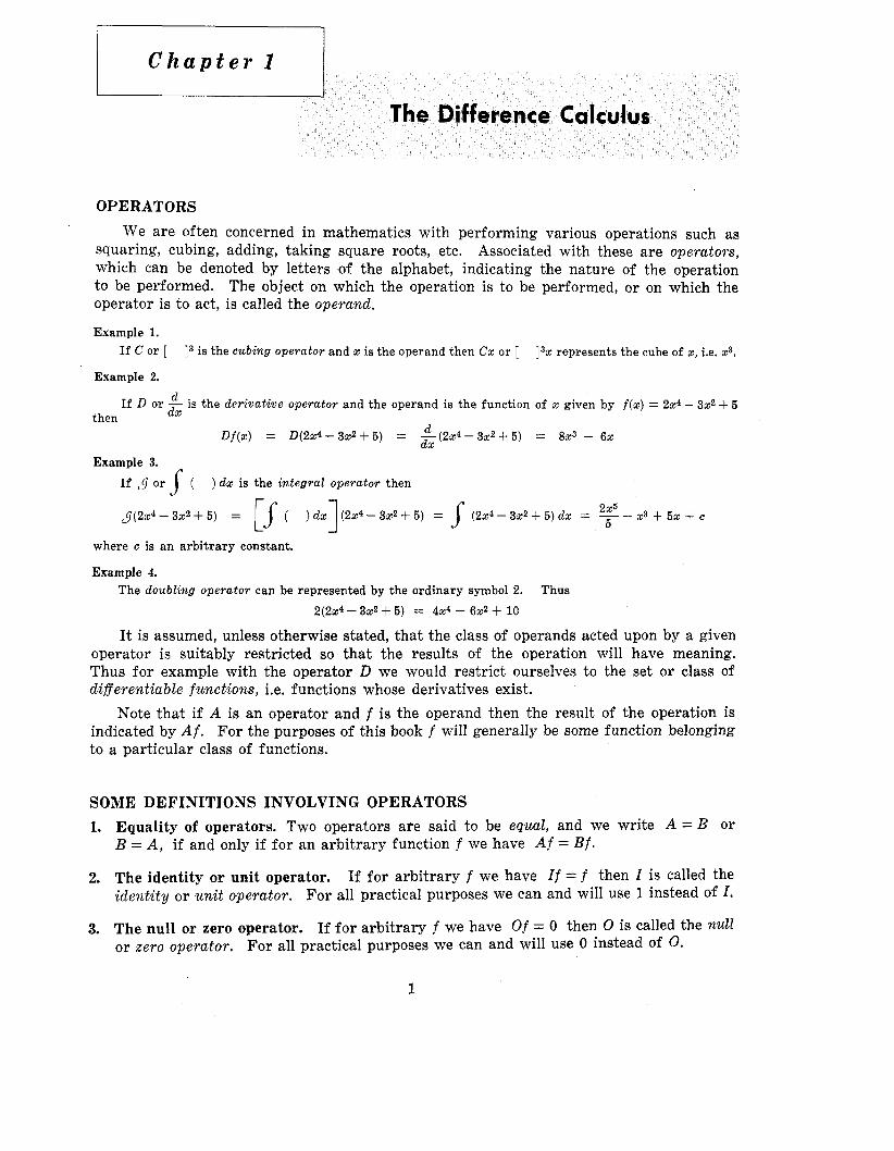
OPERATORS We are often concerned in mathematics with performing various operations such as
squaring, cubing, adding, taking square roots, etc. Associated with these are operators , which can be denoted by letters of the alphabet, indicating the nature of the operation to be performed. The object on which the operation is to be performed, or on which the operator is to act, is called the operand.
Example 1. If C o r [ 13 is the cubing operator and x is the operand then Cx or [ 13s represents the cube of x, i.e. x3.
Example 2. d
d x If D or - is the der iva t ive operator and the operand is the function of x given by f ( x ) = 2x4 - 3x2 + 5
then d
d x D f ( x ) = D ( 2 x 4 - 3 x 2 f 5 ) = -((2x4-3$+ 5 ) = 8x3 - 6%
Example 3.
If 4 o r s ( ) d x is the in tegral operator then
[J ( ) d s ] ( 2 2 ' - 3 x 2 + 5 ) = ~ ( 2 ~ 4 - 3~ + 5 ) = ( 2 & - 3 x 2 + 5 ) d s = -- 2x5 5 3 + 5 s + c 5
where c is a n arbi t rary constant.
Example 4. The doubling operator can be represented by the ordinary symbol 2.
2(2x4 - 3x2 + 5) = 4x4 - 6x2 + 10 Thus
It is assumed, unless otherwise stated, that the class of operands acted upon by a given operator is suitably restricted so that the results of the operation will have meaning. Thus for example with the operator D we would restrict ourselves to the set or class of d i f f e ren t iab le f u n c t i o n s , i.e. functions whose derivatives exist.
Note that if A is an operator and f is the operand then the result of the operation is indicated by Af. For the purposes of this book f will generally be some function belonging to a particular class of functions.
SOME DEFINITIONS INVOLVING OPERATORS 1. Equality of operators. Two operators are said to be equal, and we write A = B or
B = A, if and only if for an arbitrary function f we have Af = B f .
2. The identity or unit operator. If for arbitrary f we have I f = f then I is called the i d e n t i t y or unit operator . For all practical purposes we can and will use 1 instead of I .
3. The null or zero operator. If for arbitrary f we have Of = 0 then 0 is called the null or zero operator . For all practical purposes we can and will use 0 instead of 0.
1

THE DIFFERENCE CALCULUS [CHAP. 1 2
4.
5.
6.
7.
Sum and difference of operators. We define
( A + B ) f = A f + B f , ( A - B ) f = A f - Bf and refer to the operators A + B and A - B respectively as the s u m and d i f f e rence of operators A and B. Example 5. (C + D)xz = Cx2 + Dxz = x6 + 2 x , (C - D)x* = Cx2 - 0 x 2 = x6 - 2re
Product of operators. We define
(A*B) f = (AB)f = A ( B f ) ( 2 ) and refer to the operator AB or A B as the product of operators A and B. If A = B we denote A A or A . A as A2. Example 6. (CD)xZ = C(Dx2) = C(2x) = 8x3, C2x2 = C(Cxz ) = C ( x 6 ) = %la
Linear operators. and an arbitrary constant CY
If operator A has the property that for arbitrary functions f and g
A ( f + g ) = A f + As, A(cuf) = aAf (3) then A is called a l inear operator. a non-linear operator. See Problem 1.3.
Inverse operators. If A and B are operators such that A ( B f ) = f for an arbitrary function f, i.e. (AB)f = f or AB = I or AB = 1, then we say that B is an i nver se of A and write B = A-I = 1/A.
If an operator is not a linear operator it is called
Equivalently A- ' f = g if and only if Ag = f .
ALGEBRA OF OPERATORS
quantities if the following laws of algebra hold fo r these operators. any operators.
We will be able to manipulate operators in the same manner as we manipulate algebraic Here A, B, C denote
1-1. A + B = B + A Commutative law for sums 1-2. 1-3. AB = BA Commutative law for products 1-4. A(BC) = (AB)C Associative law for products 1-5. A(B+C) = AB + AC Distributive law
Special care must be taken in manipulating operators if these do not apply. If they do apply we can prove that other well-known rules of algebra also hold, for example the inde:c latw o r law o f exponen t s AqnAn = Am+n where Am denotes repeated application of operator A m times.
A + ( B -I- C ) = ( A + B) + C Associative law for sums
THE DIFFERENCE OPERATOR Given a function f ( x ) we define an operator 3, called the d i f f e rence operator, by
A f ( x ) = f ( x + h) - f ( x ) (4 where h is some given number usually positive and called the d i f f e rence in t e rva l or di. fei*encing in t e rva l . If in particular f ( x ) = x we have
a x = ( x + h ) - x = h or h = Ax (5)
Successive differences can also be taken. For example Azf (Z) = A [ A f ( x ) ] = A [ f ( x + h) - f ( x ) ] = f (x -k 2h) - 2 f ( X -k h) + f (x ) (6)

3 CHAP. 11 THE D I F F E R E N C E CALCULUS
We call A2 the second order d i f f e rence operator or d i f f e rence operator o f order 2. In gen- eral we define the 92th order d i f f e rence operator by
(7) A n f ( x ) = A[An-’ f (x)]
THE TRANSLATION OR SHIFTING OPERATOR We define the translat ion or s h i f t i n g operator E by
E f ( x ) = f ( x + h ) By applying the operator twice we have
E2f(lr) = E [ E f ( x ) l = E [ f ( x + h)] = f ( x + Z h ) In general if n is any integer [or in fact, any real number], we define
E ” f ( x ) = f ( x + n h )
We can show [see Problem 1.101 that operators E and A are related by
A = E - 1 o r E = l + A
using 1 instead of the unit operator I .
THE DERIVATIVE OPERATOR From ( 4 ) and (5) we have
A f ( x ) - f ( x + h ) - f ( x ) h
- - AX
where we can consider the operator acting on f ( x ) to be AIAX or Alh. The f irst order derivat ive or briefly f irs t derivat ive or simply derivat ive of f ( x ) is defined as the limit of the quotient in (11) as h or Ax approaches zero and is denoted by
if the limit exists. The operation of taking derivatives is called differen,t iation and D is the derivat ive or d i f f e ren t ia t ion operator.
The second derivat ive or derivat ive of order t w o is defined as the derivative of the first derivative, assuming it exists, and is denoted by
D”(x) = D [ D f ( X ) ] = f”(x) (63)
We can prove that, the second derivative is given by
and can in fact take this as a definition of the second derivative. Higher ordered derivatives can be obtained similarly.
THE DIFFERENTIAL OPERATOR The d i f f e ren t ia l of f irst order or briefly f irs t d i f f e ren t ia l or simply diflerential of a
function f ( x ) is defined by d f ( x ) = f ’ ( x ) A x = f’(z)h (1 5)
In particular if f ( x ) = x we have d x = Ax = h so that (15) becomes d f ( x ) = f ’ ( x ) d x = f’(x)h or df(x) = D f ( x ) d x = h D f ( x ) (1 6 )

4 T H E DIFFERENCE CALCULUS [CHAP. 1
We call d the differential operator. The second order differential of f ( x ) can be defined as d2 f (x ) = f ” ( ~ ) ( A x ) ~ = f” (x ) (dx )2 (1 7)
and higher ordered differentials are defined similarly. Note that d f ( x ) , d x =ax = h, d2f(x), (dx)2 =
necessarily zero and not necessarily small. It follows from (16) and (17) that
= h2 are numbers which are not
where in the denominator of (18) we have written (dx)2 as dx2 as indicated by custom or convention. I t follows that we can consider the operator equivalence
Similarly we shall write
RELATIONSHIP BETWEEN DIFFERENCE, DERIVATIVE AND DIFFERENTIAL OPERATORS
From (16) we see that the relationship between the derivative operator D and the differential operator d is
o r d = hD d d d x h
D = - = -
Similarly from (12) and (16) we see that the relationship between the difference operator A and the derivative operator D is
with analogous relationships among higher ordered operators. Because of the close relationship of the difference operator A with the operators D and
d as evidenced by the above we would feel that i t should be possible to develop a dif ference calculus or calculus o f differences analogous to dif ferent ial calculus which would give the results of the latter in the special case where h or Ax approaches zero. This is in fact the case as we shall see and since h is taken as some given constant, called finite, as opposed to a variable approaching zero, called infinitesimal, we refer to such a calculus as the calculus o f f inite di f ferences.
To recognize the analogy more clearly we will first review briefly some of the results of differential calculus.
GENERAL RULES OF DIFFERENTIATION
ferentiation of functions. In the following we list some of the most important ones. It is assumed that the student is already familiar with the elementary rules for dif-
m[f(x)]“-l D f ( x ) m = constant

CHAP. 11 T H E DIFFERENCE CALCULUS 5
= Duf - Dg where D, = dldu The above results can equivalently be written in terms of d rather than D. Thus for
example 11-3 becomes
d [ f ( x ) g ( x ) ] = f ( x ) dg (x ) + g ( x ) d f ( x ) = I f ( % ) g ' (x ) + g ( x ) f ' ( x ) ldx
DERIVATIVES OF SPECIAL FUNCTIONS In the following we list derivatives of some of the more common functions. The con-
stant e = 2.71828. . . is the natural base of logarithms and we write log, x as In x , called the natural logarithm. All letters besides x denote given constants.
111-1. D[c] = o 111-2. D[x"] - mxm-l 111-3. D [ ( p x + q)"] = m p ( p x + q)m-l 111-4. D[bs] = b"1nb
-
rers r cos r x -r sin r x
- 111-5. D[erz] - 111-6. D[sin Y X ] -
111-7. D[cos r x ] - 111-8. D[ln x ] = llx
- -
b > 0 , b # 1 - logb e
These results can also be written in terms of d rather than D.
becomes d(x") = mxm- 'dx
- - X 111-9. D[log, X ]
Thus for example 111-2
GENERALRULESOFTHEDIFFERENCE CALCULUS
page 4. The following results involving A bear close resemblances to the results 11-1 to 11-4 on
IV-1. A [ f ( x ) + g ( x ) ] = A f ( x ) + Ag(x) IV-2. A[a:f(X)] = a:af(x) a: = constant
IV-3. A [ f ( x ) g ( x ) ] = f ( x ) A s ( % ) + g ( x + h) A f ( x ) = g ( x ) A f ( x ) -k f ( x + h ) A g ( x ) = f ( x ) A g ( X ) + g ( x ) A f ( x ) -l A f ( x ) A s ( x )
Note' that if we divide by Ax and let AX + 0 the above results become those of 11-1 to 11-4.
FACTORIAL FUNCTIONS d
Formula 111-2 states that Dxm = mxm-l . In an effort t o obtain an analogous formula involving A we write AXm
AX ( X + h)" - xrn _ _ -
h -

6 THE DIFFERENCE CALCULUS [CHAP. 1
which however does not resemble the formula for Dxm. introduce the factorial funct ion defined by
X ( m ) = x ( x - h ) ( x - 2h) a . ( x - [m - l ] h ) consisting of m factors. The name factorial arises because in the special case x = m, h = 1 we have m(") = m(m - l ) (m - 2 ) . . a 2 - 1 = m !, i.e. factorial m.
To achieve a resemblance we
m = 1,2,3, . . . (22)
If m = 0, we define x(") = 1 , i .e. (23) x ( 0 ) = 1
For negative integers we define [see Problem l . l 8 (u ) ]
X ( - m ) = 1 - - 1 m = 1,2,3, . . . ( x + h ) ( x + 2 h ) . . ( x + mh) ( x + mh)(m) Note that as h + 0, xcm) + xm, x ( - ~ ) +. x - ~ .
Using ( Z Z ) , (23), (24) it follows that [see Problems 1.17 and 1.18(b)] for all integers m
in perfect analogy to Dxm = mxm-I and d(xm) = mxm-l d x respectively.
[see page 1031. We can also define x(") for nonintegral values of m in terms of the gamma funct ion
FACTORIAL POLYNOMIALS From (22) we find on putting m = 1,2,3, . . . I X x(1) =
x(2) = x2 - x h x(') = X' - 3x'h + 2xh2 x ( ~ ) = x4 - 6x3h + 1 l ~ ' h ' - 6xh3 x ( ~ ) = x5 - 10x4h + 35x3h2 - 50x2h3 + 24xh4
etc. If p is any positive integer, we define a factorial polynomial of degree p as +a, a0x(p) + a,x(P-l) + . .
where a0 # 0, U I , . . . , a, are constants. Using (26) we see that a factorial polynomial of degree p can be expressed uniquely as an ordinary polynomial of degree p .
Conversely any ordinary polynomial of degree p can be expressed uniquely as a factorial polynomial of degree p . This can be accomplished by noting that
1 x = x(1) x 2 = x ( 2 ) + x'l'h
I
x3 = x ( 3 ) + 3x(2)h + x(i)hz $4 = ~ ( 4 ) + 7x(3)h + 6~(2)h2 + x(l)h3
x5 = x ( ~ ) + 1 5 ~ ' ~ ) h + 25xc3)h2 + l O ~ ( ~ ) h ~ + x( l )h4
etc. uses synthetic division [see Problems 1.23-1.251.
Another method for converting an ordinary polynomial into a factorial polynomial
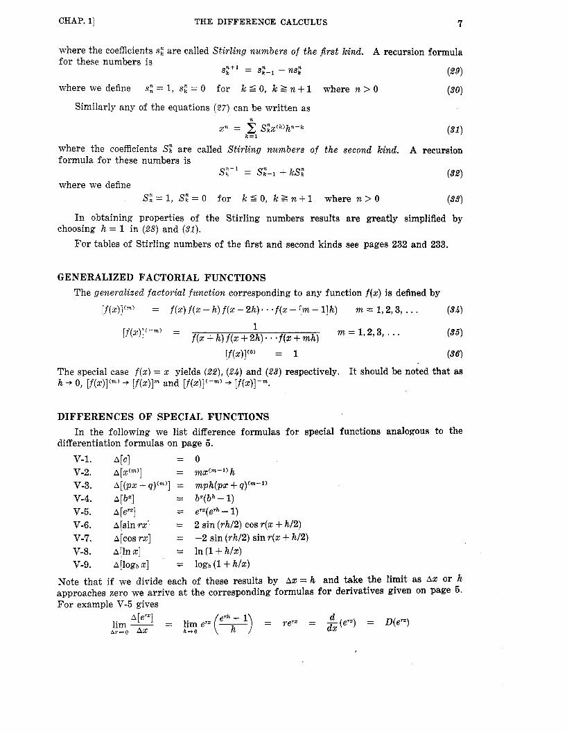
STIRLING NUMBERS Any of the equations (26) can be written as
7 CHAP. 11 THE DIFFERENCE CALCULUS
where the coefficients s: are called Stirling numbers of the first kind. A recursion formula for these numbers is
where we define
(29)
(30)
s;+l = s:-~ -ns:
s," = 1, s: = 0 for k S 0, k 2 n + 1
Similarly any of the equations (27) can be written as
where n > 0
where the coefficients S: are called Stirling numbers o f the second kind. formula for these numbers is
where we define
A recursion
Slt" = 8:-1 +kS: (32)
(33) SE = 1, Slt = 0 for k d 0, k 2 n+ 1 where n > 0
In obtaining properties of the Stirling numbers results are greatly simplified by
For tables of Stirling numbers of the first and second kinds see pages 232 and 233. choosing h = 1 in (28) and (31) .
GENERALIZED FACTORIAL FUNCTIONS The generalized factorial function corresponding to any function f ( x ) is defined by
I f (x)]'"' = f ( x ) f (X - h) f ( X - 2h) * * * f ( z - [m - l]h) m = 1,2,3, . . . (34)
The special case f ( x ) = x yields (as), (2.4) and (223) respectively. It should be noted that as h + 0, [ f ( ~ ) ] ( ~ ) + [f(x)]" and [f (x)](-") + [ f (43
DIFFERENCES OF SPECIAL FUNCTIONS
differentiation formulas on page 5 . In the following we list difference formulas for special functions analogous to the
- v-1. A[c] - v-2. A[Xcm)] -
V-4. A[b"] - V-5. A[erx] - V-6. A[sin rx] - v-7. A[cos TX] - V-8. A[lnx] - v-9. A[lOgb X] -
-
V-3. A[(pX +q)cm)] = - - - - - -
Note that if we divide each
0 mx(m-1) h mph(px + q)'m-"
bx(bh - 1) er5( erh - 1) 2 sin (rh/2) cos ~ ( x + h/2) -2 sin (rh/2) sin r(x + h/2) In (1 + h / s ) b g b (1 + h/x)
of these results by AX = h and take the limit as AX or h approaches zero we arrive at the corresponding formulas for derivatives given on page 5. For example V-5 gives

8 THE DIFFERENCE CALCULUS [CHAP. 1
TAYLOR SERIES From the calculus we know that if all the derivatives of f(x) up to order n + 1 at least
exist at a point a of an interval, then there is a number 77 between a and any point x of the interval such that
+ Rn (37) ?’(a) (x -a )2 + . , . + fy a) (x - a). f(x) = f ( 4 + ?(a) (2 - a ) + 2 ! n!
where the remainder Rn is given by f(n+l)(v) (x - U)”+l
(n + 1) ! Rn =
This is often called Taylor’s theorem or Taylor’s formula with a remainder. The case where n = 0 is often called the law of the mean or mean value theorem for derivatives.
If lim Rn = 0 for all x in an interval. then
is called the Taylor series of f(x) about x = a and converges in the interval. We can also write (39) with x = a + h so that
The special case where a = 0 is often called a Maclaurin series.
Some important special series together with their intervals of convergence [i.e. the values of x for which the series converges] are as follows.
1.
2.
3.
4.
x3 x5 x7 3 ! 5 ! 7 ! sin% 1 x - - + - - - + . . . - - m < x < m
x2 x4 x6 2! 4! 6! I - - + - - - + * . . - - m < x < m cosx =
x2 x3 x4 2 3 4 I n ( l + x ) = x - - + - - - + * * * - l < x l l
TAYLOR SERIES IN OPERATOR FORM If in (40) we replace a by x we have
f”(X)h2 + , . , f ( x + h ) = f(x) + f’(x)h +
which can formally be written in terms of operators as
= ehDf(x) E ~ ( x ) = [ l + h D + T + m h2D2 h3D3 + . * * ] f ( x )
using the series for ehD obtained from the result 1 above on replacing x by hD. This leads to the operator equivalence
(42)
or using ( l o ) , page 3, A = ehD - 1 or ehD = 1 + A (43)
E = e h D
Such formal series of operators often prove lucrative in obtaining many important results and the methods involved are often called symbolic operator methods.

CHAP. 11 THE DIFFERENCE CALCULUS 9
THE GREGORY-NEWTON FORMULA As may be expected there exists a formula in the difference calculus which is analogous
The formula is called the Gregory-Newton t o the Taylor series of differential calculus. formula and one of the ways in which it can be written is
which is analogous to (37) . The remainder R, is given by
where 17 lies between a and x. If lim Rn = 0 for all x in an interval, then (44) can be written as an infinite series which converges in the interval.
If f(x) is any polynomial of degree n, the remainder Rn = 0 for all x.
n-t m
LEIBNITZ'S RULE In the calculus there exists a formula for the nth derivative of the product of two
functions f ( x ) and g(x) known as Leibnitx's rule. This states that
q f s ) = ( f ) ( D " g ) + ( ; ) ( D f ) ( D n - W + ( ; ) ( D Z f ) ( D 9 + . * . + ( ; ) ( w ( s )
where for brevity we have written f and g for f ( x ) and g ( x ) and where
n(n - 1). . .(n - r + 1)
are the binomial coefficients, i.e. the coefficients in the expansion of (1 + x),.
- - 0 ! = 1 n ! (:) = r ! r ! ( n - r ) ! '
An analogous formula exists for differences and is given by
An( fg ) = ( f ) ( A n g ) + ( : ) (A f ) (An- lEg) 4- ( ~ ) ( A z f ) ( A n - z E ' g ) + * ' . + (:) (A" f ) (EV)
which we shall refer to 'as Leibnitx's rule f o r differences. See Problem 1.36.
OTHER DIFFERENCE OPERATORS Various other operators are sometimes used in the difference calculus although these
can be expressed in terms of the fundamental operators A and E. Two such operators are v and 6 defined by
S f ( X ) = f ( x + i ) - f ( % - k ) (49)
(50)
We call v the backward difference operator [in contrast with A which is then called the forward difference operator] and 6 the central difference operator. These are related to A and E by
See Problems 1.38 and 1.39.

10 T H E DIFFERENCE CALCULUS [CHAP. 1
Two other operators which are sometimes used are called averaging operators and are denoted by M and p respectively. They are defined by the equations
M f ( x ) = H f ( x + h) + f (43 (53)
p f (x ) = ;[++;) + f ( x - S ) ]
Some relationships of these operators to the other operators are' given by
M = *(E+1) = 1 + * A (55)
) (56) ~ = +(E1/2 +E-l/2
See Problem 1.40.
Solved Problems OPERATORS 1.1. If C is the cubing operator and D is the derivative operator, determine each of the
following.
(a) C ( 2 x + l ) ( e ) (C + 0 ) ( 4 x + 2) (h) (D2 - 2 0 + 1)(3x2 - 5~ + 4 ) ( b ) D(42 - 5x3) ( f ) ( D -i- C ) ( ~ X + 2 ) (i) (C - 2 ) ( 0 + 3)xZ (c) CD(2x - 3) (8) (Cz - 4C + l ) ( F l ) ( j ) (xCxD)x3 ( d ) DC(2x - 3) (a) c(2x + 1) = (2% + 1)3 ( d ) D C ( 2 x - 3 ) = D(22 -3)3 = 3 ( 2 ~ - 3 ) 2 * 2 6 ( 2 ~ - 3 ) 2
( b ) D(4x - 5x3) = 4 - 15x2 (c) CD(2x - 3) = C * 2 = 23 = 8
Another method. Note that from (c) and (d) i t is seen that the result of operating with CD is not the same as
operating with DC, i.e. CD # DC so that C and D are noncommutative with respect to multi- plication.
DC(2x - 3) = D(2x - 3)3 = D[8x3 - 36x2 + 542 - 271 = 24x2 - 72x + 54
( e ) (C + D)(4x + 2) = C(4x + 2) + D(4x + 2) = (4x + 2)s + 4
( f ) (D + C)(4x -t 2) = D(4x -t 2) + C(4x + 2) = 4 + (4% + The results (e ) and ( f ) illustrate the commutative law o f addition for operators C and D,
i.e. C-t D = D + C.
(9) (Cz - 4C + 1)(=1) = C Z ( e 1 ) - 4C(=l) + l ( g 1 ) = ( x - 1)3 - 4(x - 1) -t &=i 3
(h) ( 0 2 - 2 0 + 1 ) ( 3 ~ 2 - 52 + 4 ) = =
D2(3~2 - 5, + 4) - ZD(3x2- 5 2 + 4) + l ( 3 ~ 2 - 5~ + 4) 6 - 2 ( 6 ~ - 5 ) + 3 6 - 5% + 4 = 3x2 - 1 7 ~ + 20
(i) (C - 2)(U + 3 ) ~ 2 = (C - 2)[Dx2 + 3x21 = (C - 2)(2x + 3%') = C(2x + 3x2) - 2(2x + 3x2) = (2% + 3x2)3 - 2(2x + 3x2)
( j ) (xCxD)x3 = xCx(Dx3) = sCx(3x') = xC(3x3) = ~ ( 2 7 x 9 ) = 27x10
1.2. I f D is the derivative operator and f is any differentiable function, prove the operator equivalence D x - X D = I = 1, i.e. the unit o r identity operator.
We have d df d f dx dx dx ( D x - x D ) f = Dxf - xDf = - ( (x j ) - x- = x-+ f - xL'df dx = f = I f
Then for any differentiable f , (Dx - xD)f = If = 1 or Dx - X D = Z = 1.

11 CHAP. 11 T H E DIFFERENCE CALCULUS
1.3. Prove that (a) the cubing operator C is a nonlinear operator while (b ) the derivative operator D is a linear operator. (a) If f and g are any functions we have
Then in general since ( f + g)3 f f 3 + g 3 i t follows that C ( f 4- g) ;f Cf + Cg so that C cannot be a linear operator, i.e. C is a n o n l i n e a r opera tor .
( b ) If f and g a r e any differentiable functions, we have
C ( f + 9) = ( f + s )3 , C f + cg = f 3 + g3
Also if a is any constant, then D ( a f ) = a - df = aDf d x Then D is a linear operator.
1.4. (a) If C denotes the cubing operator, explain what is meant by the inverse operator C-'. ( b ) Does C-' exist always? (c) Is C-l unique? Illustrate by considering C-l(f3). ( a ) By definition B = C-l is that operator such tha t C B f ( x ) = f(x) or CB = I = 1, the unit
or identity operator. Equivalently C - l f ( x ) = g ( x ) if and only if C g ( x ) = f ( x ) o r [ g ( x ) ] 3 = f(z), i.e. g(x) is a cube roo t of f ( x ) . Thus C-l is the o p e r a t i o n o f taking cube roo ts . As a particular case C-l(8) is the result of taking cube roots of 8.
( b ) I f f(x) is real, then C - l [ f ( x ) ] willalways exist but may o r may not be real. For example if C-l(8) is denoted by x then x3 = 8, i.e. (x - 2 ) ( x 2 + 2 x + 4) = 0 and x = 2, -1 * fi i so that there a r e both real and complex cube roots. The only case where C - l f ( x ) is always real when f ( x ) is real is if f(x) = 0.
(c ) It is clear from ( b ) t h a t C-1f (x ) is not always unique since for example C-l(8) has three differ- ent values. However if f ( x ) is real and if we restrict ourselves to real values only, then C - l f ( z ) will be unique.
If f ( x ) is complex, C - l f ( x ) always exists.
Thus if we restrict ourselves to real values we have for example C-l(8) = 2 .
THE DIFFERENCE AND TRANSLATION OPERATORS 1.5. Find each of the following.
(a) 4 2 x 2 + 3 X ) ( d ) E3(3X - 2 ) (9) (A + 1)(2A - 1)(x2 + 2x + 1) ( b ) E(4x - X 2 )
(C) A2(X3 - X 2 )
(a) A(2& + 3%) =
( e ) (2A2 4- A - 1 ) ( X 2 + 23: + 1) ( f ) (E2 - 3E + 2)(2"Ih + X)
[ 2 ( ~ + h)2 + 3 ( x + h)] - [222 + 3x1
(h) (E - 2)(E - 1)(2"Ih + X) '
= 2x2 + 4 h z + 2h2 t 3x + 3h - 2x2 - 3% = 4hx + 2/22 + 3 h
( b ) E ( 4 x - x2) = 4 ( x + h) - (x + h)2 = 4 2 + 4 h - x2 - 2 h z - h2
= [ 3 ( x + h)2h + 3 ( x + h)h2 -t h3 - 2 h ( z + h) - h2] - [3x2h + 3xh3 + h3 - 2hx - h2]
(c) A2(x3 - 22) = A [ A ( d - &)I = A [ { ( % + h)3 - (X + h)2} - (x3 - xz)] = A[3x2h + 3xh2 + h3 - 2hx - h2]
= 6h% + 6h3 - 2hZ
(d) E 3 ( 3 ~ - 2 ) = E Z E ( 3 x - 2 ) E2[3(x + h) - 21 = E . E[3(x + h) - 21 = E [ 3 ( x + 2 h ) - Z ] = 3 ( x + 3 h ) - 2
( e ) (2A2 + A - I)(& + 2% + 1) = 2A2(x2 + 2% f 1) + A(x2 + 2% f 1) - 1(x2 + 2 2 + 1) = ~ A [ { ( x + h)2 + 2 ( x f h) f 1} - { X 2 + 2% + I}]
+ [{(x + h)2 t 2 ( x + h) + l} - {x2 + 2% -I l}] - 5 2 - 2% - 1 = 2 A [ 2 h 2 + h2 -k 2h] + [2h% + hz + 2/21 - X 2 - 2% - 1 = 2 [ { 2 h ( x + h) + h2 + 2 h } - {Zhs + h2 + 2h}]
+ 2 h x i- h2 + 2 h - x2 - 2s - 1 = 5/22 + 2 h x + 2 h - 2 2 - 2 x - 1
Note t h a t we use 1 in 2Az + A - 1 instead of the unit o r identity operator I.
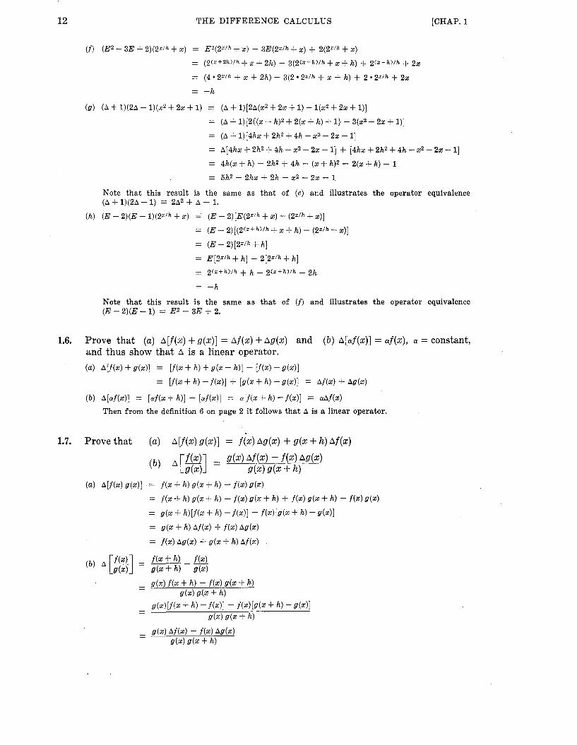
12 THE D I F F E R E N C E CALCULUS [CHAP. 1
(f) (E2 - 3E + 2)(2z/h + X) = E2(25/h + X) - 3E(2z/h + X) + 2(2”/h + X) = (2(X+2h)/h + x + 2h) - 3 ( 2 ( ~ t h ) / h + x + h) + 2 ( ~ + h ) / h + 22
= (4 2xlh + x + 2h) - 3(2 2x/h + x + h) + 2 2z/h + 22 = -h
= (A + 1)[2A(x2 + 2% 4- 1) - l(x2 + 2% + I)]
= (A + 1)[2{(x -t h)2 4- 2(2 + h)
= (A + 1)[4hx + 2h2+ 4h - ~ 2 - 2x - 11 = A [ 4 h ~ + 2h2 + 4h - x2 - 2% - 11 + [4hz + 2h2 + 4h - x2 - 22 - 11
(9) (A + 1)(2A - 1)(x2 + 2x + 1)
1) - 3(x2 + 22 + l)]
= 4h(x + h) + 2h2 + 4h - (x + h)2 - 2(x + h) - 1 5/22 + 2hx + 2h - 2 2 - 2x - 1 =
Note t h a t this result is the same a s tha t of ( e ) and illustrates the operator equivalence (A + 1)(2A - 1) zz 2A2 + A - 1.
(h) (E - 2)(E - 1)(2z/h + x) = (E - 2)[E(25’h + x) - (2z/h + x)] (E - 2)[(2(%+h)/h + x + h) - (2Z’h + x)] (E - 2)[2X/h + h]
=
=
= E[2Z/h + h] - 2[25/h + h] X I 2(zth) /h + h - 2(z+h)/h - 2h
= -h
Note t h a t this result i s the same as that of (f) and illustrates the operator equivalence ( E - 2 ) ( E - l ) = E z - 3 E + 2 .

CHAP. 11 THE DIFFERENCE CALCULUS 13
1.8.
1.9.
1.10.
1.11.
Prove formulas (a) V-4 ( b ) V-5 (c) V-6, page 7. (4 A[bZ] = b Z t h - b x = &(bh-1 )
( b ) A[eTZ] = eT(Zth) - eTZ = eTZ(eT'h- 1)
(4 A[sinrx] = sinr(x + h) -
sin el - sin e2 = 2 on using the trigonometric formula
with e l = r ( x + h) and e2 = rx .
Prove that AE = EA, i.e. the operators A and E are commutative with respect to multiplication.
We have for arbitrary f(z) A E f ( x ) = A [ E f ( x ) ] = A [ f ( ~ + h ) ] = f ( x + 2 h ) - f ( z + h )
E ~ f ( x ) = E [ ~ ( z + ~t) - f ( ~ ) ] = f ( x + 2 h ) - f(x + h) Then A E f ( x ) = E A f ( x ) , i.e. A E = E A .
We have for arbitrary f(z) A f b ) = f(x -t h) - f(s) = E f b ) - f ( x ) ( E - l ) f ( z )
Thus A = E - 1 where we use 1 instead of the unit or identity operator I .
We have for arbitrary f(x) E f ( x ) = f(z+ h) = fb) + [fb+ h) -fb)] = fb) + A f ( x ) = ( 1 + A ) f ( x )
Note that this illustrates the fact that we can treat operators A and E as In particular we can transpose the 1 in A = E - 1 to obtain
Thus E = 1 + A . ordinary algebraic quantities. E = l + A .
We have for arbitrary f(s) A z f ( s ) = A [ A f ( s ) ] =
- - - - - - - - - -
Thus A2 = ( E - 1 ) 2 = E2 - 2 E + 1.
Obtain a generalization of Problem 1.10 for an where n is any positive integer. Method 1.
Usinn the fact that A and E can be manipulated as ordinary algebraic quantities we have by
n! are the binomial coefficients. where (:> = r ! ( n - r ) !
By operating on f(x) the result (I) is equivalent to
~ n f ( x ) = f ( x + nh) - f ( x + (n - 1)h) + f ( x + (n - 2)h ) - * * + (-l)nf(s)

14 THE DIFFERENCE CALCULUS
Method 2. Assume that
~ n f ( x ) = f(x + n h ) - f ( x + (n- l ) h ) + + ( - l )n f (x )
[CHAP. 1
is true for a positive integer n, i.e. assume the operator equivalence
Then operating on both sides of (2 ) with A we have
= f(x + (n + 1)h) - f ( x + nh) - A n t l f ( z ) [f(x + nh) - f(x + (n - l ) h ) ] (3 + ( - l ) " [ f ( x + h) - f(41 + ...
- . . . + ( - l )"+' f (x)
or since [see Problem 1.1051 (:) + (A) = (Z) n + l n + l
we have An+'f(x) = f ( x + (n + 1)h) -
+ ( - l )"+l f (x ) (8) - ... It follows that if (2 ) is true then (3) is true, i.e. if the result is true for n i t is also true for n+ 1. Now since ( 2 ) is true for n = 1 [because then (2) reduces to A f ( z ) = f(x + h) -f(x)], it follows that it is also true for n = 2 and thus for n = 3 and so on. I t is thus true for all positive integer values of n. The method of proof given here is called mathematical induction.
1.12. Prove that (a) E-l f (x ) = f ( x - h), (b) E-nf(x) = f(x - nh) for any integer n. (a) By definition if E - l f ( x ) = g(x), then Eg(s) = f(z), i.e. g(z + h) = f(x) or g(s) = ffz - h)
Thus E - l f ( x ) = f(z - h).
( b ) Case 1. If n is a negative integer or zero, let n = -m where m is a positive integer or zero. on replacing x by x - h.
Then Emf(x) = f(s+mh), i.e. E-n f (x ) = f ( s - n h ) Case 2. If n is a positive integer, then by definition if
E-nf(x) = g(x) then Eng(x) = f(z) or g ( x + n h ) = f(x)
E-nf(s) = g(z) = f (s-nh) Then replacing x by x - nh we have
In general we shall define Enf(.x) = f ( x + n h )
for all real numbers n.
THE DERIVATIVE AND DIFFERENTIAL OPERATORS
1.13. A d lim - ( (zx2 + 3x) = - ( 2 x 2 + 3x) = 4x + 3
a 2 lim 4 ( x 3 - x 2 ) = 7(x3-x2) = 6x - 2 AX+O A x dx
Show that (a) A x r ~ A x ax
( b )
directly from the definition. (a) From Problem 1.5(a) we have since h = Ax
4hx + 2h2 + 3h - 4x + 2h + - A Ax h -(2x2+32) =
A d lim -(2x2+32) = lim ( h x + 2 h + 3 ) = 42 + 3 = ;EjE(2x2+ 3s) Ax-rO AX h r O
Then

CHAP. 11 THE DIFFERENCE CALCULUS 16
( b ) From Problem l.S(c) we have since h = Ax and h2 = AX)^
A2 6 h z ~ + 6h3 - 2hz = 6 ~ + 6 h - 2 - ( x 3 - x 2 ) = Ax2 h2
Then lim - ( x 3 - x 2 ) A2 = lim (6x + 6h-2) = 6x - 2 = d 2 2 ( x 3 - ~ 2 ) dz
The results illustrate the fact that ~ ~ o ~ f ( x ) An = ~ f ( x ) . dn
h-0 AZHO Ax2
Note the operator equivalence
dxn. The notation D = z, D2 = a, . . . , Dn = dn can also be used. Strictly
d" However by custom we leave off the
lim - = - d d2 An dn bz-ro Axn
dn An and as - An speaking we should write - as - Axn (Ax)" (dx)n *
parentheses in the denominator,
dxn
1.14. Find (a) d(2x2+3x), ( b ) d2(z3-x2) .
(u) By definition, using dx = Ax = h we have
d dx d ( 2 ~ 2 + 3 ~ ) = - ( 2 ~ 2 + 3 ~ ) dx = (42 + 3) dx = ( 4 ~ + 3)h
(b) By definition, dZ(x3 - $2) = - ( ~ 3 CP - x 2 )(dx)z = (62 - 2 ) ( d ~ ) 2 = ( 6 s -2)hZ dx2
1.15. Prove that D [ f ( x ) g(x)] = f(x) D g ( x ) + g(x) Df(x). From Problem 1.7(u) we haye on dividing by h = Ax
A A A Ax - [ f (4 9(4] = f(4 9(4 + 9@ + h) 1: f(4
Then taking the limit as h = Ax+O we have
d d d [ t ( x , 9(x)] = f ( 4 ;i;E d4 + 8(4 f ( 4
which gives the required result on writing d / d x = D.
sin 8 d 1.16. Use Problem 1.8(c) and the fact that lim 7 = 1 to prove that ds sin T X = T cos z.
8-0
From Problem 1.8(c) we have since Ax = h
A - [sin rx] Ax 2 sin (rh/2) cos r(x + h/2)
h
= r * l * c o s r x
r cosrx - -
We have used here the theorem familiar from the calculus that the iimit of a product of functions is equal to the product of the limits of the functions whenever these limits exist.

16 THE DIFFERENCE CALCULUS [CHAP. 1
FACTORIAL FUNCTIONS 1.17. If xCm) = x(z - h)(x - 2h) * . (x - [m - llh), m = 1, 2, 3, . . ., prove that -xCm) = A
AX m x ( m - l ) or equivalently A d r n ) = mx(m-l)h where h = Ax.
We have Az(lil) = (z + h)(Vl) - x ( m )
L1 = ( z + h ) ( x ) ( z - h ) . . . ( ~ - [m-2]h) - ~ ( x - h ) ( x - 2 h ) . . . ( x - - [ m - l ] h )
= x(x - h) . * .(x - [m - 2]h) {(x + h ) - (x - [m - ljh)} - - mx(m-l)h
Note t h a t for m = 1 this formally reduces to A x ( 1 ) = z(O)h
However since Ax(” = Ax = h we are led to define d o ) = 1.
1.18. (a) Motivate the definition of x ( - ~ ) , m = 1 ,2 ,3 , . . . , given on page 6 . defihition on page 6 prove that
( b ) . Using the
( a ) From the definition of z(m) for “m = 1 , 2 , 3 , . . . we have Z ( m ) = z(z - h) * . . ( 5 - [m - l ] h )
x ( m + l ) = z ( z - h ) . . . ( x - m h )
so t h a t z ( m + l ) = x(m)(x-mh)
If now we formally put m = -1 in this last result, we are led t o X ( 0 ) = x(-l)(x.+ h)
Using d o ) = 1, from Problem 1.17 we are thus led t o define
x ( -1 ) = I
2(-1) = x ( - - 2 ) ( $ + 2h)
2 - h Similarly, putting m = -2 in (1) we find
so t h a t we are led to define 1 - x ( - 1 )
x + 2h x ( -2 ) = - - (x + h)(x + 2h)
Proceeding in this way we a r e thus led to define
x(-m) = m = 1 ,2 ,3 , 1 ( X + h)(z + 2h). - . (z + mh)
as on page 6.
( b ) We have Ax(-rn) = (%+ h)(-m) - % ( - m )
1 - 1 - - (x+2h)(z+3h) . . . ( z+ [ m + l ] h ) ( x+h) (x+2h) . . . ( x+mh)
1 - ’1 [ 1
- -mh
- - -mx(-m-l)h
- - ( x+2h)* . ’ ( z+mh) x + ( m + l ) h a + h
- (x + h)(x + 2h) . (x + mh)(x + [m + 11 h)
- -mx( -m - 1) A x ( - m )
Ax - - or equivalently
Note tha t the results of this problem and Problem 1.17 enable us t o write for all integers m A x ( m ) __ = m z ( m - l ) or ~ x ( m ) = mx(m-l)h Ax

CHAP. 11 THE DIFFERENCE CALCULUS 17
1.19. If m is any integer and c is any constant prove that
( b ) Since AX = h we have from part (a)
Method 2. A[cx(m)] = cAx(m) = mchx(m-1)
Since A and thus A f A x are linear operators we have
and the required result follows a t once from Problems 1.17 and 1.18.
A A 1.20. Find (a) ax [ 3 ~ ( ~ ) ] , (b) A [ ~ O X ( ~ ) ] , (c) ax [ 5 ~ ( - ~ ) ] , (d) A [ - ~ z ( - ~ ) ] expressing all results
in terms of h. From the results of Problem 1.19 we have
(a) f-[3x(4)] = 4 - 3253) = l2x(3) = 124% - h)(x -2h)
( b ) ~ [ 1 0 ~ ( 3 ) 1 = 3.10~(2)h = 3ohx(2) = 3 0 h ~ ( x - - )
A 1.21. Find (a) ( 2 ~ ' ~ ) - 3d2) + x - 4), ( b ) - 2 ~ ' ~ ) - 5d-l) 1.
By Problem 1.19 and the fact that A and thus AlAx are linear operators we have A Ax
A Ax
(a) - (2d4) - 3 d 2 ) + x - 4) = 8d3) - 62") + 1
(6) - ( 3 ~ - 2 - 2x(2) - 5xc-l)) = (-62(-3) - &(l) f 5x(-Z))h
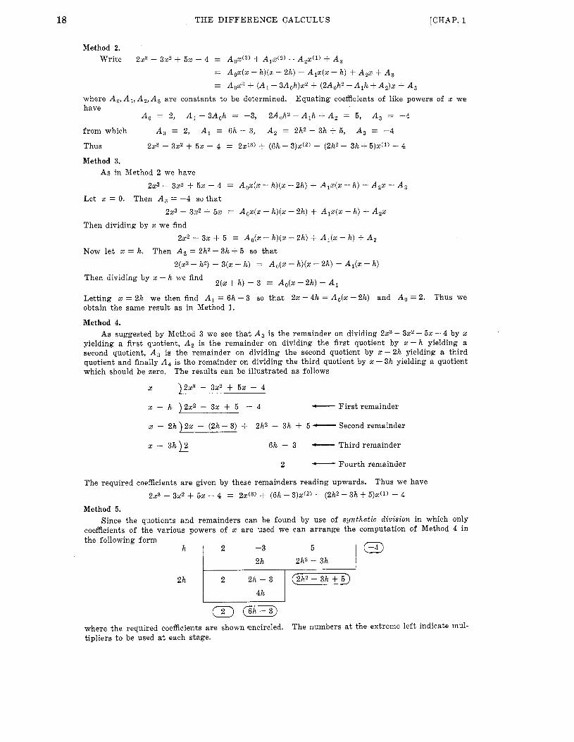
1.23. Express 2x3 - 3x2 + 5% - 4 as a factorial polynomial in which the difference interval is h. Method 1.
From page 6 we have 2 x 3 - 3~ + 52 - 4 = 2(q3) + 3x(2)h + .(1)-2) - 3 ( ~ ( 2 ) + ~ ( 1 ) h ) + 5 ~ ( 1 ) - 4
= 2x(3) + (6h - 3)2(2) 4- (2h2 - 3h + 5)x(') - 4
18 T H E DIFFERENCE CALCULUS [CHAP. 1
Method 2. Write 2x3 - 3 x 2 + 5 x - 4 = A , d 3 ) + Alx(2) + A,x( l ) + A ,
= A,.(% - h)(z - 2h) + A,%(% - h) + AZx + A3 = A,x3 + ( A , - 3A0h)x2 + (2Aoh2 - A,h + A,)% + A ,
where A,, A , , A,, A , are constants to be determined. have
Equating coefficients of like powers of x we
A , = 2 , A1 - 3Aoh -3, 2Aoh2- Alh + A , = 5 , A3 = -4
from which A , = 2 , A , = 6h - 3, A2 = 2 h 2 - 3 h + 5 , A , = -4
Thus
Method 3.
2x3 - 3x2 + 5% - 4 = 2x(3) + (6h - 3 ) x ( 2 ) + (Zhz - 3h + 5 ) x ( 1 ) - 4
As in Method 2 we have 2x3 - 3x2 + 5x - 4 = A,%(% - h)(x - 2h) + A,%(% - h) + A,% + A3
Let x = 0. Then A , = -4 so tha t
2x3 - 3x2 + 5% = A,x(x - h)(x - 2 h ) $- A l x ( x - h) + A2x Then dividing by % we find
2x2 - 3% + 5 = A,(% - h ) ( x - 2h) + A,(% - I L ) - A , Now let x = h. Then A , = 2h2 - 3 1 ~ + 5 so tha t
Z(x2 - h2) - 3 ( 2 - h) = Ao(x - h ) ( x - 2h) + A,(% - h)
Then dividing by x - h we find 2 ( x + h) - 3 = A,(% - 2 h ) + A ,
Letting x = 2h we then find A , = 6h - 3 so tha t 2x - 4h = A,(% - 2 h ) and A , = 2. Thus we obtain the same result as in Method 1.
Method 4. As suggested by Method 3 we see t h a t A , is the remainder on dividing 2x3 - 3x2 + 5% - 4 by x
yielding a first quotient, A , is the remainder on dividing the first quotient by x-h yielding a second quotient, A , is the remainder on dividing the second quotient by x - 2 h yielding a third quotient and finally A , is the remainder on dividing the third quotient by x - 3 h yielding a quotient which should be zero. The results can be illustrated as follows
X )2%3 - 3x2 + 5 x - 4
x - h ) 2 x 2 - 3 x + 5 - 4 C- Firs t remainder
x - 2 h ) 2 2 + ( 2 h - 3 ) + x - 3 h k 6h - 3 C- Third remainder
~~
2h2 - 3h + 5 C- Second remainder
2 - Fourth remainder
Thus we 2x3 - 3x2 + 5 x - 4 = 2 x ( 3 ) + (6h - 3 ) 2 ( 2 ) + (2h2 - 3h + 5 ) x ( 1 ) - 4
The required coefficients a r e given by these remainders reading upwards.
Method 5.
have
Since the quotients and remainders can be found by use of synthetic divisiolt in which only coefficients of the various powers of x are used we can arrange the computation of Method 4 in the following form
h 1 2 -3 5
I 2 h 2 h 2 - 3h j 2 h ~ 2 2h4;3 1 @-)
(2> (m) where the required coefficients a r e shown encircled. tipliers to be used at each stage.
The numbers a t the extreme left indicate mul-

T H E DIFFERENCE CALCULUS 19 CHAP. 11
1
2
3
1.24.
1 0 0 1 1
1 1 1 2 2 6
1 3 7 3
-
-
Express 2x3 - 3x2 + 5% - 4 as a fakorial polynomial in which the differencing inter- val h = 1.
In greatly reduces
this case any of the methods of Problem 1.23 can of course be used and the results a re simplified because h is replaced by 1. For example Method 5 which is the simplest method to the following
2 4
3
2x(x - 1)(x - 2) + 3x(x - 1) + 4% - 4
2x3 - 3x2 + 5x - 4 2x3 - 6x2 + 4x + 3x2 - 3% + 4x - 4
1.25. Express x 4 + x - 2 as a factorial polynomial in which h = 1. We must be careful in using Method 5 of Problem 1.23 to introduce zero coefficients where
needed. Thus we have the following
Thus x4 + - 2 = d 4 ) + ~ ~ ( 3 ) + 7x(2) + 2 x c ~ ) - 2
Check. I L . ( ~ ) + 6 ~ ( 3 ' + 7 ~ ( " + ZX"' - 2 =
= = x 4 + x - 2
X(X - l)(x - 2 ) ( ~ - 3) + 62(x - 1 ) ( ~ - 2) + ~ X ( X - 1) + 2 x - 2 x4 - 6x3 + 11x2 - 6% + 6x3 - 18x2 + 12% + 7x2 - 7x + 22 - 2
1.26. Show that if m = 1 ,2 ,3 , . , . (ax + b)'") = (ax + b)(ax + b - ah)(ax + b - 2ah). * (ax 3. b - mah + a h )
The result follows from definition (34) , page 7, on letting f(x) = ax + b so that
f(x - h) = U ( X - h ) + b = ax 4- b - ah, f ( x - 2 h ) = a(% - 2 h ) + b = ux + b - Zah, . . ., f ( x - [m - l ]h) = ~ ( x - [m - l ]h) + b = rtx + b - ~ [ m - l ] h = ax + b - mah 4- ah
1.27. Show that if m = 1,2,3, . . . 1
(ax + b + ah)(ax + b + 2ah) . (ax + b + maG (ax + b ) ( - m ) =
The result follows from definition (35) , page 7, on letting f ( x ) = ax + b so tha t
f ( x + h ) = a ( x + h ) + b = ax + b + ah, f ( x + 2h) = a(% +2h) + b = ax + b + Zah, . . ., f ( x + m h ) = a(x +mh) + b = ax + b + mah

20 THE DIFFERENCE CALCULUS [CHAP. 1
(a) Letting h = 1, a = 2, b = 9 and m = 3 in Problem 1.26 we have
(2s + 9)(3) = (2x + 9)(2s + 7)(2x + 5 )
( b ) Letting h = 1, a= 3, b = -5 and m = 4 in Problem J.27 we have
1
(3s - 2)(3s + 1 ) ( 3 ~ f 4)(3s 4- 7) (3s - 5)(-4' =
STIRLING NUMBERS 1.29. Derive the recursion formula (29), page 7 , for Stirling numbers of the first kind.
Using h = 1 in (28), page 6, we can write the result as
where we take
since the series (1) is actually finite and
s z = 0 for k 5 0, k 2 n + l where n > 0
s; = 1
since both sides of (1) are polynomials of degree n.
Replacing n by n + 1 in (I) we have $ ( n + l ) = sjt+lxk
k = - x
Now if h = 1 we have X ( n + l ) = X(n)(s-n)
Then substituting (I) and (a) into (4) we have
Equating coefficients of xk we find as required
s;+' = s : - ~ -ns:
1.30. Derive the recursion formula (32), page 7 , for Stirling numbers of the second kind.
where we use ( J I ) , page 7, with h = 1. Since both sides are polynomials of degree n we have
S;=O for kS 0, k 2 n S 1 where n > 0 (2)
so that the series (1) is actually finite. From ( I ) we have on replacing n by n -t 1

CHAP. 13 T H E D I F F E R E N C E CALCULUS 21
Since ~ n + l = X, e x , we have from (1) and (4.)
But
Thus
Equating coefficients of d k ) we find as required
SE+l = S;- l+kS;
1.31. Show how the method of Problem 1.25 can be used to obtain Stirling numbers of the second kind by using the polynomial f(x) = x4.
We use the same method as tha t of Problem 1.25 as indicated in the following
1 1 0
1
0
1
0
1 l o 1
1 6
It follows tha t
and the Sticling numbers a r e 1, 6, 7, 1.
%4 = %(4) + 6%(3) + 72(2) +
THE GREGORY-NEWTON FORMULA AND TAYLOR SERIES 1.32. Prove the Gregory-Newton formula (44), page 9, for the case where f(x) is a poly-
nomial and a = 0. If f(z) is a polynomial of degree n we can write it as a factorial polynomial, i.e.
f(x) = A , + A , z ( l ) + A2x(2) + A3x(3) + * * + Anx(n) (1 )
Then

22 THE DIFFERENCE CALCULUS [CHAP. 1
Putting x = 0 in the above equations we find
A , = f(O), A , = ..., A , = --
which we can agree to write as
Using these in (1) we obtain the required formula for a = 0.
If we use the same method above with 2 replaced by x - a and then put z = a the more general formula (44) on page 9 is obtained.
1.33. Prove the Gregory-Newton formula with a remainder given by (44) and (QS), page 9.
Let p,(x) denote the polynomial of degree n as determined in Problem 1.32. Writing
p,(s) = a,@ + ap--l + *. . + a, we see that it has n + 1 coefficients a,, a,, . . .,a,. It follows that if f(z) is some given function we can determine these n + 1 coefficients uniquely in terms of the values of f(z) at n + 1 different values of 2, say xo, x,, . . . , x,. We shall suppose that this is done. In such case
f ( zo) = P,(zo), f(xJ = P,(s~), . . * 3 f ( 4 = Pn(xn) (1)
. . . . . . . . . . . I . . . . . . . . .
f(%) = P,(Xn) + g(x,)
dxo) = 0, = 0, . . ., dx,) = 0
It thus follows that unless g(2) is identically zero [in which case f(2) is a polynomial and we will have f ( z ) = p,(z)J we must have
($1
(4 )
Then using (1) we see that
g(2 ) = K(x) (x - x,)(z - El). ' *(x - Z,) Thus from (Z),
f(x) = Pn(z) + K ( x ) (x - X O ) ( X - $0) * * ( z - 2,)
To obtain K ( s ) in terms of f(x) let us consider the function
U ( t ) = f(t) - p , ( t ) - K ( z ) ( t - x,)(t - 5,)' * ' ( t - an) (5 )
It follows from (4) that this equation has the n + 2 roots t = 2, x,, z,,. . .,a,. Then by Problem 1.117 the (n+ 1)st derivative of U(t ) , i.e. U(n+')( t ) , is zero for at least one value, say t = 7, between the smallest and largest of 2, xo, xl, . . . , x,. But from (5 )
U(n+"(t) = f ( " + I ) ( t ) - (n + l)! K ( s ) (6)
since p(;fl)(x) = 0. Putting t = 7 in (6) and setting it equal to zero i t thus follows that

CHAP. 11 THE DIFFERENCE CALCULUS
X
0
1
2
3
4
23
f (4 A f ( 4 A2f (2) A3f (4 A4f (2)
-4
0
10
38
96
6
18
30
4
10
28
58
0 12
12
Since we can choose any values for $0, xl, . . . , x,, let us choose
Then $0 = a, 5 1 = a + h , 5 2 = a + 2 h , ..., x, = a + n h
which is Gregory-Newton's formula with a remainder.
1.34. Work Problem 1.24 by using the Gregory-Newton formula. For any polynomial f(x) of degree n we have
or using Ax = h = 1,
f(x) = f(0) + AfdO)x(l) + - A2f(0) x ( 2 ) + . . . + T r n ( n ) A"f(0) 2!
Now f(z) = 2x3 - 3 x 2 + 5z - 4 so that
f (o ) = -4, f(1) = 0, f(2) = 10, f(3) = 38, f(4) = 96 Then
Af(o) = f(1) - f(0) = 4, Af(1) = f(2) - f(1) = 10,
Af(3) = f(4) - f(3) = 58
Af(2) = f(3) - f(2) = 28
From these we find
A2f(o) = Af(1) - Af(0) = 6, A2f(l) = Af(2) - Af(1) = 18,
Azf(2) = Af(3) - Af(2) = 30
Similarly,
and finally
From these we see that
A3f(0) = Azf(l) - Azf(0) = 12, A3f(l) = A2f(2) - Azf(1) = 12
~ 4 f ( o ) = ~ 3 f ( i ) - ~ 3 j ( o ) = o
f(0) = -4, Af(0) = 4, Azf(0) = 6, A3f(0) = 12, A4f(0) = 0
and so (I) becomes
in agreement with the result of Problem 1.24.
223 - 322 + 6s - 4 = -4 + 4x(1) + 3s(2) + 2d3)

P
24 T H E DIFFERENCE CALCULUS [CHAP. 1
1.35. Show how to arrive a t the Gregory-Newton formula for the case where h = 1, u = 0 by using symbolic operator methods.
We have for any value of n [see Problem 1.121
Enf(u) = f(u+nh) (1 1
EZf(0) = f (4 (3)
Then in particular if we choose u = 0, n = x, h = 1, this becomes
Using E = 1 + A in (2) and expanding formally by the binomial theorem, ( 2 ) becomes
f(z) = Exf(0) = (1 + A)"f(O)
The result is the same as the infinite series obtained from (4.4), page 9, with h = Ax = 1 and a = 0.
Extensions to the case where h f 1, u f 0 can also be obtained symbolically [see Problem 1.831.
LEIBNITZ'S RULE 1.36. Prove Leibnitz's rule for the nth difference of a product of functions.
Let us define operators El and E, which operate only on f(z) and g(2) respectively, i.e.
. E,[ f (x ) g(x)] = f(x + h) dx), E,[f(X) g b ) ] = f(x) Q(x + h)
Then EIEz[ f (x ) g(z)] = f(x + h) g(x + h) = E [ f ( x ) g(x)] so tha t E = E,E,. operators Al, A, with El , E , respectively, i.e. El = 1 + Al, E , = 1 + A,.
and so
Associate the difference Then
A = E - 1 = EIE, - 1 = (1 +A1)E, - 1 = Ez + AIEz - 1 = A2 + PIE,
A"[fg] = (A2 + A 1 E d n [ f g ]
1.37. Find A"[xzua"]. Let f = x2, g = ax. Then by Leibnitz's rule we have
OTHER DIFFERENCE OPERATORS 1.38. Find (a) v ( x 2 + 2 x ) , ( b ) S ( x 2 + 2 x ) .
(a) V(x2 + 2%) = [x2 + 2x1 - [(2 - h)2 + 2(2 - h)]
= x 2 + 2 x - [,Z-2hx+h2+22-2h]
= 2hs + 2h - h2
CHAP. 11 T H E DIFFERENCE CALCULUS 25
( b ) 6 ( X 2 + 2 X ) = [ ( X + ; ) ' + 2 ( x + ; ) ] - [ ( X - ; ) 2 + 2 ( x - ; ) ]
) h2 ) - ( x 2 - K x + - + 2 x - h k 2 = (9 + hx + r+ 2% + 11 4
= 2hx + 2h
1.39. Prove that (a) v = AE-' = E - ~ A = 1 - E-1 (b ) 8 = ,73112 - E-112 = ~E- l /2 = VE112
(a) Given any function f ( x ) we have vf(%) = f(x) - f ( ~ - h ) = A f ( x - h ) = AE-'f(%)
so tha t V = AE-L Similarly
vf(X) = f(z) - f(z - h) = E - l [ f ( x + h) - f(x)] = E-lAf(x) so tha t V = E - l A . Finally
V f ( X ) = f(x) - f ( x - h) = f(x) E - I f ( % ) = (1 -E- ' ) f (x ) so t h a t V = 1 - E-1.
( b ) Sf($) = f (. + ;) - f (. - ;) = E1/2f(z) - E-'/Zf(x) = ( E 1 / 2 - E - m ) f ( X )
so t h a t 6 = E 1 / 2 - E-1/2 . Similarly
6 f ( x ) = f ( ~ + k ) - f ( ~ - k ) = A f ( 2 - a ) = A.?C-1/2f(~)
so t h a t 6 = AEd1I2 . Finally
Sf(%) = f ( x + k) - f(x - a) = Of (x + ;) = VE1/2f(x)
so t h a t 6 = V E 1 / 2 .
1.40. Find (a) M(4x2 - 8x), ( b ) p(4x2 - 8%).
(a) M ( 4 x 2 - 82) = 4[4(% + h)2 - 8 ( ~ + h) + 42' - 8x1 4x2 + 4 h ~ + 2h2 - 8% - 4h
MISCELLANEOUS PROBLEMS 1.41. If f(x) = aoxn + ulxn-l+ - * +a,, i.e. a polynomial of degree n, prove that
(a) A n f ( x ) = n!aoh" (b ) An t l f (%) = 0, An"f(x) = 0, , . . Method 1.
We have A ~ ( z ) = [ao(. 4- h)n + u,(z+ + + a,] - + C L ~ X ~ - ~ f + a,]
= [aonxn-lh + terms involving xn-2, 5%--3, . . . 7 It follows t h a t if A operates on a polynomial of degree n the result is a polynomial of degree n - 1. From this we see t h a t An!(%) must be independent of x, i.e. a constant, and so Antlf(x) = 0, A n * 2 f ( ~ ) = 0, . . ., which proves ( b ) . To find the constant value of Ant(%) note that we need only consider the term of highest degree. Thus we have
Azf(x) = [ U o n ( x h)n-'h + . * ] - [aonxn-lh + . ' ' 1 = ao.[(. + hp-1- z n - l l h + * ' .
a,?&[(% - l )xn-Zh + . * ' ] h + . . . aon(n - 1)Xn-Zhz + . * *
= =

26 T H E D I F F E R E N C E CALCULUS [CHAP. 1
Proceeding in this manner we see finally tha t
A f l f ( x ) = a,n(n- l ) (n-2) . . . ( l )hn = n!aohn
For another method see Problem 1.84.
Method 2.
have Since every polynomial of degree n can be written as a factorial polynomial of degree n, we
~ 0 % " + a l ~ n - 1 + * . + a, = boxfn) + b r ~ ( n - 1 ) + + b,
Equating coefficients of xn on both sides we find bo = a,. The required result then follows since
1.42. Prove that
We have
Now from Problem 1.41 with h = 1 we have for T > n
while if r = n,
Thus the required result follows.
1.43. Show that (a) ArOn = 0 if r > n, ( b ) AflOfl = n !
( a ) Putt ing x = 0 in (2) of Problem 1.42 we have for T > n, ArOn = 0.
(a) Putt ing x = 0 i n (3) of Problem 1.42 we have for = n, Anon = n !
We call ATOn the differences of zero.
1.44. Prove Rolle's theorem: If f ( x ) is continuous in a S x S b , has a derivative in a < x < b , and if f(a) = 0, f ( b ) = 0, then there is a t least one value 7 between a and b such that f'(7) = 0.
We assume t h a t f(x) is not identically zero since i n such case the result is immediate. Suppose then t h a t f(x) > 0 f o r some value between a and b. Then i t follows since f(x) i s continuous tha t i t a t ta ins its maximum value somewhere between a and b, say at q. Consider now
a f o = f ( 7 + h) - f ( 7 ) Ax h
where we choose h = Ax so small t h a t 7 + h is between a and b. Since f(7) is a maximum value, i t follows tha t Af(2)lA.x 2 0 for h < 0 and Af(x)/Ax 5 0 for h > 0. Then taking the limit a s h + 0 through positive values of h, we have f'(7) S 0, while if the limit is taken through negative values of h, we have f ' ( 7 ) 2 0. Thus f ' ( 7 ) = 0. A similar proof holds if [(z) < 0 for some value between a and b.

27 CHAP. 11 T H E DIFFERENCE CALCULUS
1.45. (a ) Prove the mean value theorem for derivatives: If f(x) is continuous in a 5 x S b and has a derivative in a < x < b, then there is at least one value TJ between a and b such that
( b ) Use (a) to show that for any value of x such that a d x 5 b,
f(x) = f(a) 3- (3 - a)f’(rl) where 7) is between a and x.
(c) Give a geometric interpretation of the result.
(a,) Consider the function
(1 1 f ( b ) - f ( a ) F ( x ) = f(’) - f ( a ) - ( X - a ) b - a
From this we see t h a t F(a) = 0, F(b) = 0 and tha t F ( x ) satisfies the conditions of Rolle’s theorem [Problem 1-44]. Then there is at least one point 7 between a and b such tha t F’(q) = 0. But from (1)
(2 ) f ( b ) - f (4 F’(x) = f’(x) - ~- b - a
so tha t
or
( b ) Replacing b by x in (3) we find as required
where q is between x and a.
Taylor series can be proved by extensions of this method.
f ( x ) = f (4 + (x - a)f’(v) (4 )
Note t h a t ( 4 ) i s a special case of Taylor’s series with a remainder for n = 1. The general
(c) The theorem can be illustrated geo- metrically with reference to Fig. 1-2 where i t is geometrically evident tha t there is at least one point R on the curve y = f(x) where the tangent line PRQ is parallel to the secant line ACB. Since the slope of the tangent line at R is f’(v) and the slope of the secant line is [ f ( b ) - ! (a)] /@ - a) , the result fol- lows. It is of interest to note t h a t F(x ) in equation (1) represents geometri- cally RC of Fig. 1-2. In the case where f ( a ) = 0, f ( b ) = 0, RC represents the maximum value of f(x) in the interval a S x 5 b .
A
X a 7 b
X a 7 b
Fig. 1-2

28 T H E DIFFERENCE CALCULUS [CHAP. 1
Supplementary Problems OPERATORS 1.46. Let d = [ 12 be the squaring operator and D the derivative operator. Determine each of the
following, (4 6(1+Vz) (e) ( 6 2 + 2 d - 3)(2x - 1) (i) x3D3&(2 + 1)
(b) ( 2 d + 3 D ) ( ~ 2 - X) (f) (D + 2 ) ( d - 3 ) ~ ' (I.) (.d - d W d X 2
(4 dW3X + 2) (9) (@J - 3)(D + 21x2 (4 D d ( 3 x +2) (h) (xD)3&(2 + 1)
1.47. (a) Prove t h a t the operator of d-l and determine whether i t always exists and is unique.
Prove tha t @ = C2 where d and C a r e the squaring and cubing operators respectively.
Let eJ be the squaring operator and a: be any real number. (a) Explain the meaning of the operators ad and &a. Illustrate by a n example.
Is the operator ( x D ) ~ the same as the operator x4D4?
Prove t h a t (a) D2x - xD2 = 20, (b) 0 3 2 - 5 0 3 = 302. prove it.
of Problem 1.46 is a nonlinear operator. ( b ) Explain the significance
1.48.
1.49. ( b ) Do the operators CY and obey the commutative law?
1.50.
1.51.
Justify your answer.
Obtain a generalization of these results and
THE DIFFERENCE AND TRANSLATION OPERATORS 1.52. Find each of the following.
(b) E ( & F - z ) (f) (xE2 + 2xE + 1)x2 (j) ( x A E ) ~ ~ ~ (c) A2(2x2-5x) (9) A2E3x (d) 3E2(~2 + 1) (h) (3A + 2)(2E - l)s2
Determine whether discuss the significance of the results.
Prove t h a t E is a linear operator.
Determine whether (a) A2 and (b) Ez a r e linear operators. E n ? Explain.
1.56. Verify directly tha t A3 = (E - l ) 3 = E3 - 3E2 + 3E - 1.
1.57. Prove formulas (a) V-7, ( b ) V-8, (c) V-9 on page 7.
1.58.
(a) 4 ( 2 ~ - 1)2 (e) (A + 1)2(x + (i) (2E - 1)(3A + 2 ) ~ z
1.53. (a) (E - 2)(A + 3) = (A + 3)(E - Z), (b) (E - %)(A + 3%) = (A + 3x)(E - 2) and
1.54.
1.55. Do your conclusions apply to An and
Prove tha t the commutative law for the operators D and A holds (a) with respect to addition, ( b ) with respect to multiplication.
(a) Does the associative law with respect to multiplication hold D, A and E? (b) Does the commutative law with respect to multiplication hold for D and E?
Show t h a t
1.59.
A A Z + O AX
1.60. (a)
(b) lim - [ ~ ( 2 - x ) ] = -[x(2-x)] = -2
lim - [x(Z - x)] = D[%(2 - %)I = 2(1 - X)
A2 d2 Ax-0 Ax2 dx2
directly f rom the definition.
Find (a) 4 x 3 - 3x2 + 2% - l), (b) d2(3X2 + 2% - 5) .
Prove t h a t D [ f ( x ) + g(x)] = Df(x) + D g ( x ) giving restrictions if any.
1.61.
1.62.

CHAP. 11 T H E DIFFERENCE CALCULUS 29
A sin e lim - [cos r x ] = --r sin rx by using the fact t h a t lim 7 1.64, Prove t h a t = 1. Ar-tO Ax 6-0
A A Z + O Ax
1.65. Prove t h a t lim - [br] = bx In b stating assumptions made.
1.66.
1.67.
Prove equation ( I h ) , page 3, giving suitable restrictions.
Obtain a relationship similar to tha t of equation (U), page 3, between D3f(x) and A3f(x)/Ax3.
1.70. Express each of the following as factorial polynomials for h = 1 and for h f 1.
(a) 3x2 - 5% + 2, ( b ) 2x4 + 5x2 - 4% + 7.
A A2 1.71. Find (a) ( 2 4 - 2x2 + 5x - 3), (b) - (x4 - 2x2 + 5x - 3). Ax2
1.72. Express each of the following as a product of suitable factors using the indicated values of h. (a) (2s - 1)(4) if h = 2, (b) (32 + 5)(3) if h = 1, (c) (4x - 5)c-Z) if h = 1, (d) (5x + 2)-(4) if h = 2.
1.73. Write each of the following as a factorial function. (a) (3% - 2)(3x + 5 ) ( 3 ~ + 12),
x(z + 2)(z + 4) '
(b) (2 + 2 x ) ( 5 + 2 ~ ) ( 8 + 22)(11+ 2%)
1 1 (d) (2% - 1)(2x + 3)(2z + 7 ) ( 2 x + 11)
A Prove t h a t - (px + q ) ( m ) = mp(px + q)(m-l) for (a) m = 0,1,2, . . . , ( b ) m = -1, -2, -3, . . Ax 1.74.
2 2 - 1 21c + 1 (2% + 3)(22 + 5)(22 + 9) (a) (s + 2)(x + 4)(x + 6) ' 1.75. Express in terms of factorial functions
STIRLING NUMBERS 1.76. Obtain Stirling numbers of the first kind s t for n, k = 1 , 2 , 3 by using the recursion formula (2%
page 7.
1.77. Obtain Stirling numbers of the second kind SE for n, k = 1,2,3 using the recursion formula (a@, page 7.
1.78. Find S i for k = 1,2, . . ., 6 by using the method of Problem 1.25.
1.79. Prove t h a t s ; + s ; + " ' + s ; = 0
and illustrate by referring to the table of Stirling numbers of the first kind in Appendix A, page 232.
1.80. Prove t h a t (a) 8; - 8; + 53" - . * * + (-1)n-h; = ( - l ) n - b t !
(b) + Is;/ + * . ' + = n!
THE GREGORY-NEWTON FORMULA AND TAYLOR SERIES 1.81. Express each of the following as factorial polynomials for the cases h = 1 and h f 1 by using
the Gregory-Newton formula. (a) 3x2 - 5 s + 2, (b) 2x4 + 5x2 - 4 s + 7.
30 T H E DIFFERENCE CALCULUS [CHAP. 1
1.82. Under what conditions is the remainder R, in ( 4 5 ) , page 9, equal to zero?
1.83. Show how to generalize Problem 1.35 by obtaining the Gregory-Newton formula for the case where h P 1 , U P O .
1.84. Prove t h a t An[aOxn + U1xn-' + * * + a,] = YL! aohn by using the Gregory-Newton formula.
1.85. Obtain the Taylor series expansion for f ( x ) from the Gregory-Newton formula by using a limiting procedure.
1.86. Obtain the Taylor series expansions ( a ) 1, ( b ) 2, ( c ) 3 and (13) 4 on page 8 and verify the intervals of convergence in each case.
LEIBNITZ'S RULE 1.87. Use Leibnitz's rule to find A3(x2 2.) if h = 1.
1.88. Find An(xa").
1.89. Find An(x2aX).
1.90. Obtain Leibnitz's rule for derivatives from Leibnitz's rule for differences by using an appropriate limiting procedure.
OTHER DIFFERENCE OPERATORS 1.91. If f(x) = 2x2 + 3x - 5 find (a ) V f ( x ) , ( b ) S f ( % ) , (c) V 2 f ( x ) , ( d ) S Z f ( x ) .
1.92. Evaluate ( V 2 -3VS + 2S*)(x2+ 2x ) .
1.93. Prove t h a t ( a ) V2 = (~E-1)2 = A2E-2, ( b ) V n = AnE-n.
1.94. Determine whether the operators V and S are commutative.
1.95. Demonstrate the operator equivalence E = (i + d-)'. 1.96. Prove tha t V A = AV = S2.
1.97. Is it t rue t h a t (a) lim - " = - d y ( b ) lim 3 = 7 Explain. 6x- toSx dx ' 6 x - ~ S X " d x n '
1.98.
1.99.
Show t h a t
Determine whether ( a ) M and ( b ) p commutes with A, D and E.
(a) M = +(l + E ) = E - +A, ( b ) p = M/E1/2.
1.100. Show t h a t (a) A = pS + @2, ( b ) A 2 m t 1 = Em[pSZm+l + J - S m + 2 2 I.
MISCELLANEOUS PROBLEMS 1.101. (a) If A and B are any operators show tha t ( A - B)(A + B ) = A2 - B2 + AB - BA.
conditions will it be t rue tha t ( A - B ) ( A + B ) = A2- B2? and ( b ) by considering (A2 - D2)x2 and (A - D ) ( A + D)x2.
( b ) Under what ( c ) Illustrate the results of par ts (a)
p h 1.102. Prove t h a t (a ) A sin ( p x + q ) = 2 sin- sin [ p x q f $ ( p h 4- T ) ] 2
Ph A cos ( p x + q ) = 2 s i n F cos [ p x + q + $ ( p h + TI ] ( b )

CHAP. 11 THE DIFFERENCE CALCULUS 31
1.103.
1.104.
1.105.
1.106.
1.107.
1.108.
1.109.
1.110.
1.111.
1.112.
1.113.
1.114.
1.115.
1.116.
1.117.
Prove that ( a ) Am sin (px + q) = r 2 sin r p x + q + 2 m (ph + T ) ] L J L
1 ( b ) Am cos (px + q) = px 4- q + m ,(ph+ T)
Use Problem 1.103 t o show that
dm ( b ) ~ C O S X = cos
dm (a) dxm sinx = sin
and thus complete the proof of Problem 1.11, Method 2.
sec2 x tan h d dx
(a ) Show that A tan x = and ( b ) deduce that - t a n s = sec2x.
h
1 - tan x tan h
and d and ( b ) deduce that tan-1 x = -
x2 + 1 (a) Show that A tan-1x = tan-lx2 + hx +
d X a dx tan-1- a = - x2 + u2'
(a) Show that A sin-1 x = (x + h) d m - x d l - (X + h)2.
( b ) Deduce from (a) that - sin-lx = ~
d 1 d X 1 dx dx a d m '
and -sin-'- = -
1 1 Prove that for h = l (a) 8: = -Dnx(k)I n! x=o ' ( b ) S: = aAkxn!z=O
Prove that 5': = 5 (-l)p(E) pn and illustrate by using the table on page 233. k! p=o
Show that the index law for factorial functions, i.e. x ( ~ ) x ( ~ ) = x ( m + n ) , does not hold.
Prove that
and discuss the relationship with Leibnitz's rule.
Prove that n(n - 1) n(n - l)(n - 2) n! = nn - n(n-1)" + 2!(n-2)" - 3! (n-3)" + a ' *
h2D2 I h3D3 h4D4 + . . . Show that (a) A = hD +x 3! +4!
h5D5 31h6Ds + . . . ( b ) ~2 = h2Dz + h3D3 + hh4D4 + 7 4- 360
3h4D4 5h5D5 3hsDs 903h7D7+ . , (c) A3 = h3D3 + - 2 +-+-+- 4 4 2520
Find (a) A2(3x3-2x2+ 4x-6), ( b ) A3(x2+ x)2 by using Problem 1.115 and compare results by direct evaluation.
If U ( t ) is the function defined by (5 ) of Problem 1.33, prove that U("+l) ( t ) = 0 for at least one value t = 9 between the smallest and largest of x, xo, xl, . . . , x,. [Hint. Apply Rolle's theorem successively.]

1 C h a p t e r 2 I
Applications of the Difference Calculus
SUBSCRIPT NOTATION Suppose that in f(x) we make the transformation x = a + kh from the variable x to
the variable k. Let us use the notation y = f (x) and
yk = f(a + kh) (4 It follows that [see Problem 2.11
Ayk = Ykti-yk, Eyk = Y k t l
' and so as on page 3 a = E - l or E = l + A
Using this subscript notation it is clear that a unit change in the subscript k actually corresponds to a change of h in the argument x of f(x) and conversely. In addition all of the basic rules of the difference calculus obtained in Chapter 1 can be written with subscript notation. Thus for example formula IV-4, page 5 , becomes
Also since x = a + k h becomes x = k if a = 0 valid if we replace x by k and put h = 1. Thus for
example equations (22) and (25), page 6, become respectively
(5) kCm) = k (k - l ) ( k - 2) * * * ( k - Wt 4- I), = ~ , k ( ~ - ' )
It should be noted that k need not be an integer. In fact k is a variable which is discrete or continuous according a5 x is. An important special case with which we shall be mainly concerned arises however if k = 0, 1,2, . . . so that the variable x is equally spaced, i.e. x = a, a + h, a + 2h, . . , . In such case we have yo = f(a), y1 = f(a + h), yz = f(a + 2h), . . . .
DIFFERENCE TABLES A table such as that shown in Fig. 2-1 below which gives successive differences of
24 = f ( x ) for x = a, a+h, a+%, . . ,, i.e. Ay,A2y,A3y, . . ., is called a diflerence tabZe.
Note that the entries in each column after the second are located between two successive entries of the preceding column and are equal to the differences between these entries. Thus for example A2y1 in the fourth column is between Ay1 and Ay2 of the third column and A2y1 = Ayz - Ay1. Similarly A3y2 = a2y3 - A2yz.
32

CHAP. 21
X
1
2
3
4
5
6
X
y = f(x) = 23 AY *2Y A3Y A4Y
1
8 12
27 18 0
64 24 0
125 30
216
7
19 6
37 6
61 6
91
U
a + h
a + 2h
a + 3h
a + 4h
a t 5h
33 APPLICATIONS OF THE DIFFERENCE CALCULUS
Y AY A2Y A3y A4Y A5Y
Fig. 2-1
Example 1. The difference table corresponding t o y = f(x) = 2 3 for x = 1,2 , . . ., 6 is as follows.
Fig. 2-2
The first entry in each column beyond the second is called the leading d i f ference for that column. In the table of Fig. 2-1 the leading differences for the successive columns are A y ~ , h ~ y o , ~ ~ y ~ , . . . . The leading differences in the table of Fig. 2-2 are 7,12,6,0. It is often desirable also to include the first entry of the second column called a leading d i f ler - ence of order zero.
It is of interest that a difference table is completely determined when only one entry in each column beyond the first is known [see Problem 2-41.
DIFFERENCES OF POLYNOMIALS It will be noticed that for f(z) = x3 the difference table of Example 1 indicates that the
third differences are all constant, i.e. 6, and the fourth differences [and thus all higher differences] are all zero. The result is a special case of the following theorem already proved in Problem 1.41, page 25.
Theorem 2-1. If f(x) is a polynomial of degree n, then Anf(x) is a constant and Ant l f (x ) , ~ . + ~ f ( x ) , . . . are all zero.

34 APPLICATIONS O F T H E DIFFERENCE CALCULUS
X
Y
[CHAP. 2
X P
YP
xo X1 . . .
Yo Yl . . .
GREGORY-NEWTON FORMULA IN SUBSCRIPT NOTATION If we put x = a + kh in the Gregory-Newton formula (44) on page 9, it becomes
(6) Anf (a ) Wn) + Rn
n ! + A f ( a ) k ( l ) + Az f ja )k (2 ) + . . . 2 ! f ( a + k h ) = f ( a ) + 1!
where the remainder is given by hn+ I f ( n + I ) ( 9 ) k(n+ 1)
R, = (n + 1) ! the quantity 7.1 being between a and a + kh and where
k“’ = I t , k(2) = k ( k - l), k‘3’ = k j k - l ) ( k - 2), . . . In subscript notation (6) can be written as
If An+lyo,Ant2y0, . . . are all zero, then R n = 0 and y k is a polynomial of degree n in k .
GENERAL TERM OF A SEQUENCE OR SERIES
of terms in a sequence or series [see Problems 2.8 and 2.91. The Gregory-Newton formula is often useful in finding the general law of formation
INTERPOLATION AND EXTRAPOLATION
various values of x as indicated in the table of Fig. 2-3. Often in practice we are given a table showing values of y or f ( x ) corresponding to
Fig. 2-3
We assume that the values of x are increasing, i.e. xo < $1 < + < xP. An important practical problem involves obtaining values of y [usually approximate]
corresponding to certain values of x which are not in the table. It is assumed of course that we can justify seeking such values, i.e. we suspect some underlying law of formation which may be mathematical or physical in nature.
Finding the [approximate] value of y corresponding to an untabulated value of 2 b e t w e e n xo and x p is often called in terpola t ion and can be thought of as a “reading between the lines of the table”. The process of obtaining the [approximate] value of y correspond- ing to a value of x which is either less than xo or greater than xp, i.e. lies outside the table, is often called extrapolation. If x represents the time, this can involve a problem in predic t ion or f o recas t ing .
Suppose that the x values are equally spaced and the nth differences of y or f ( x ) as obtained from the table can be considered as small or zero for some value of n. Then we can obtain a suitable interpolation or extrapolation formula in the form of an approximating polynomial by using the Gregory-Newton formula. See Problem 2.11.
If the x values are not equally spaced we can use the Lagrange in terpola t ion f o r m u l a [see page 381.
Because formulas for interpolation can also in general be used for extrapolation we shall refer to such formulas collectively as in terpola t ion f o r m u l a s .

35 CHAP. 2: APPLICATIONS OF THE DIFFERENCE CALCULUS
X
a - 3h
a - 2h
a - h
a
a + h
a + 2h
a + 3h
CENTRAL DIFFERENCE TABLES In the table of Fig. 2-1 it was assumed that the first value of x was x = a, the second
x = a + h, and so on. We could however have extended the table backwards by considering x = a - h, a- 2h, . . . . By doing this we obtain the table of Fig. 2-4 which we call a central diflerence table.
Y AY A2Y A3Y A4Y A5Y A6Y
Y-3 AY-3
76-2 A%-3
AY-2 A3Y-3
Y-1 A2Y - 2 A4Y - 3
Yo A'Y-1 A * Y - ~ AOY - 3 AYO A3y - A5y-,
Y1 A2Yo A4y - AY 1 ASY 0
Y2 A2Y 1
AY2
AY-1 A3y - 2 A'y - 3
Y3
The table of Fig. 2-4 can also be written equivalently in terms of central differences as shown in Fig. 2-5.
~
X
a - 3h
a - 2h
a - h
a
a + h
a + 2h
a + 3h
Y-3
Y-2
Y-1
Yo
Y l
YZ
Y3
6 Y -5 /2
sY-3/2
SY-1/2
8Y1/2
s y 3 / 2
6Y.5/,
Fig. 2-5
Note that the entries of this table can be related to those in the table of Fig. 2-4 by simply using the operator equivalence 6 = AE-l12 on page 9. Thus for example,
S3y,3/2 = (AE-1 '2)3y-3/2 = A3E-3 /2 y - 3 / 2 = n 3 y - 3
Other tables can be made using the backward difference operator V.

' 36 APPLICATIONS O F T H E DIFFERENCE CALCULUS [CHAP. 2
GENERALIZED INTERPOLATION FORMULAS In using the Gregory-Newton formula ( 6 ) or (8) for interpolation, greater accuracy is
obtained when x or a + kh is near the beginning of the table rather than near the middle or end of the table. This is to be expected since in this formula use is made of the leading differences A f ( a ) , Az f (a) , . . . .
To obtain more accuracy near the middle or end of the table we need to find interpolation formulas which use differences near the middle or end of the table. The following are formulas which do this. All of these formulas are exact and give the same result when the function is a polynomial. If it is not a polynomial, a remainder or error term can be adaed. The results can also be expressed in terms of the operators V or 6 of page 9.
For the purposes of completeness and reference we include in the list the result (8).
1. Gregory-Newton forward difference interpolation formula.
2. Gregory-Newton backward difference interpolation formula.
3. Gauss' interpolation formulas.
4. Stirling's interpolation formula.
5. Bessel's interpolation formula.
ZIG-ZAG PATHS AND LOZENGE DIAGRAMS There exists a simple technique for not only writing down all of the above interpolation
formulas but developing others as well. To accomplish this we express the central difference table of Fig. 2-4 in the form of a diagram called a lozenge diagram as shown in Fig. 2-6 below. A path from left to right such as indicated by the heavy solid line in Fig. 2-6 or the heavy dashed line is called a zig-zag path.

CHAP. 21 APPLICATIONS O F T H E DIFFERENCE CALCULUS 37
( k + 3)'"/3!
/ A4Y--4 ' , P L Y - 3
\ . Y - 2
I 1 , (k - l)(2)/2!
Fig. 2-6
The following rules are observed in obtaining an interpolation formula.
1.
2.
3.
4.
5.
6.
A term is to be added whenever any column containing differences is crossed from left to right. The first column in Fig. 2-6 is to be considered as containing differences of order zero.
If the path enters a difference column from the left with pos i t ive slope [as for exam- ple from yo to Ay-1 in Fig. 2-61, the term which is to be added is equal to the product of the difference and the coefficient which is indicated directly below the difference.
If the path enters a difference column from the left with negat ive slope [as for example from Ay-1 to A2y-l in Fig. 2-61, the term which is to be added is equal to the product of the difference and the coefficient which is indicated directly above the difference.
If the path enters a difference column with zero slope [as for example from 1 to A ~ O in Fig. 2-61, the term which is to be added is equal to the product of the differ- ence and the arithmetic mean of the coefficients directly above and below the difference.
If the path crosses with zero slope a column between two differences [as for example in the path from A ~ O to ~ ~ y - 1 in Fig. 2-61, the term which is to be added is equal to the product of the coefficient between the two differences and the arithmetic mean of the two differences.
A reversal of path changes the sign of the corresponding term to be added.

38 APPLICATIONS OF THE DIFFERENCE CALCULUS [CHAP. 2
LAGRANGE'S INTERPOLATION FORMULA
differences of y are not small or zero the above interpolation formulas cannot be used. In case the table of Fig. 2-1 either has nonequally spaced values of x or if the nth
In such case we can use the formula
(x - Xl)(X - xz) * * * (x - x,) (x-xo)(x-x2)~~'(x-x,) Y = yo(xo-xl)(xo-xz)' . ' ( X O - - X , ) + y1 (x1- xo)(x1- x2) * . a (x1- x p )
(x-xo)(x-xl).'.(x-x,--l) (x, - xo)(xp - Xl) * (x, - xp-1) + YP + . . .
which is called Lagrange's interpolation formula [although it was known to Euler].
nth differences are small or not. Note that y is a polynomial in x of degree p. The result holds whether the values XO, 21, . . . , x, are equally spaced o r not and whether
TABLES WITH MISSING ENTRIES Suppose that in a table the x values are equally spaced, i.e. x = a, a + h, a + 2h, . . .
and that all the corresponding entries f ( x ) , except for a few missing ones, are given. Then there are various methods by which these missing entries can be found as shown in Prob- lems 2.28-2.30.
DIVIDED DIFFERENCES If a table does not have equally spaced values of x, it is convenient to introduce the
idea of divided differences. Assuming that the values of x are XO, XI, XZ, . . . and that the function is f ( x) we define successive divided differences by
etc. They are called divided differences of orders 1,2 ,3 , etc. We can represent these differ- ences in a divided difference table as in Fig. 2-7.
Various other notations are used for divided differences. For example f(xo, xi, $2) is sometimes denoted by [xo, XI, x2] or A[xo, XI, $21.

CHAP. 21 APPLICATIONS O F T H E D I F F E R E N C E CALCULUS 39
The following are some important results regarding divided differences.
1. The divided differences are symmetric. For example
f(x0, $1) = f(x1, XO), f(xo, $1, $2) = f (x1, XO, $2) = f ( x z , XO, XI), etc.
2. If f ( x ) is a polynomial of degree n then f(x, $0) is a polynomial of degree n - 1, f(x, XO, xl) a polynomial of degree n - 2, . . . . Thus f(x, xo, XI, . . . , G-I) is a constant and f(x, XO, 21, . . ., X n ) = 0.
3. Divided differences can be expressed in terms of first differences. For example,
f (4 f (xd + f (4 (xo - x1)(xo - $2) + ($1 - xo)(x1- xz) (xz - xo)(x2 - Xl)
f ( x0 , x1, $2) =
NEWTON'S DIVIDED DIFFERENCE INTERPOLATION FORMULA From the above results we obtain
f(x) = f ( x 0 ) + (x - xo)f(xo, X l ) + (x - xo)(x - x1)f(xo, $1, x2)
+ * a * + ( X - - O ) ( X - - X ~ ) . . . ( X - - ~ - ~ ) ~ ( X ~ , X ~ , . . . , ~ n ) S R ( I d )
where n n (x - Xk) = (x - xo)(x - $1) ' * (x - xn)
k = O
and 7 is some value between the smallest and largest of x, XO,XI, . . .,xn. The result (12) can be written as
where p3,(x) is a polynomial in x of degree n often called an interpolat ing polynomial.
f ( 4 = pn(x) + R (15)
INVERSE INTERPOLATION We have assumed up to now that the values of x in a table were specified and that we
wanted to interpolate [or extrapolate] for a value of y = f ( x ) corresponding to a value of x not present in the table. It may happen however that we want a value of x corresponding to a value y = f(x) which is not in the table. The process of finding such a value of x is often called inverse interpolat ion and a solution for x in terms of y is often designated by x = f - l ( y ) where f- ' is called the inverse function. In this case the Lagrange interpolation formula or Newton's divided difference formula are especially useful. See Problem 2.38 and 2.39.
APPROXIMATE DIFFERENTIATION From the formula ehD = 1 + A [equation (.43), page 81 we obtain the operator equivalence
A' A3 A4 f - - -+ ... 3 4
1 D = h l n ( l + A ) =
by formally expanding In (1 + A ) using the series on page 8.
table. from (16): We find for example
By using (16) we can obtain approximate derivatives of a function from a difference Higher derivatives can be obtained by finding series expansions for D2, D3, . . .

40 APPLICATIONS O F T H E DIFFERENCE CALCULUS [CHAP. 2
Use can also be made of different interpolation formulas to find approximate derivatives. In these cases a remainder term can be included enabling us to estimate the accuracy.
Solved Problems SUBSCRIPT NOTATION 2.1. If y = f(x) and y k = f ( a + kh), show that
(a) A y k = y k + l - y k (b) E y k = y k + l (c) E = l + a
Since Yk = f(a + kh) we have
(a) A u k = Af(a+kh) = f ( a + k h + h ) - f ( a + k h ) = Y k t i - y k
(b) E Y k = f (U+kh) = f ( a + k h f h ) = U k t l
(c) From parts (a) and ( b ) , Y k + A Y k = E'& O r (1 + A)Yk = E l 4 k
Then since Yk is arbi t rary we have E = 1 + A.
DIFFERENCE TABLES 2.3. Let f(x) = 2x2- 7% + 9 where x = 3,5,7,9,11.
The required table is shown in Fig, 2-8 below. Note tha t in column 2 the various values of f ( s )
Set up a table for the differences of f ( 4 .
a r e computed from f(x) = 239 - 7x + 9. Thus fo r example f(5) = 2(5)2 - 7(5) + 9 = 24, etc.

CHAP. 21
X
3
5
7
9
11
APPLICATIONS O F T H E DIFFERENCE CALCULUS
ld = f (4 AY A2Y A3Y A42/
6 18
24 16 ' 34 0
58 16 0 50 0
66 108 16
174
41
2.4. Find the numerical values corresponding to the letters in the following difference table where it is assumed that there is equal spacing of the independent variable x.
$4 AY A% A3Y A4Y A5Y
A F
B -1 G M
3 J -3 H N -5
C K P -2 4
D L Z
E
Fig. 2-9
Star t ing at the r ight end i t is clear tha t P- (-3) = -5 or P = -8. Similarly we find in succession the equations 4 - N = P or N = 12, N - M = -3 o r M = 15, J - (-1) = M or J = 14, K - J = N or K = 2 6 , L - K = 4 or L = 3 0 , Z- ( -2)=L or Z = 2 8 , - 2 - H = K or H = - 2 8 , H - G = J or G=-42, G - F = - 1 or F = - 4 1 , 3 - B = G or B = 4 5 , B - A = F or A = 8 6 , C - 3 = H or C = - 2 5 , D - C = - 2 or D = - 2 7 , E - D = I or E = l .
The final difference table with the required numbers replacipg letters is as follows:
Y AY A22/ A3Y A416 A52/
I 86
-41 45 -1
-42 15 14
-28 12 -25 26 -8
-2 4
28
-b 3
-27 30
1
Fig. 2-10
The problem illustrates the fac t that a difference table is completely determined when one From the manner in which the letters were obtained i t is clean entry in each column is known.
that they can each have only one possible value, i.e. the difference table is unique.

42 APPLICATIONS O F T H E DIFFERENCE CALCULUS [CHAP. 2
2.5. By using only the difference table of Problem 2.3 [and not f ( x ) = 2x2-7x+9] find the values of 3 = f ( x ) for x = 13,15,17,19,21.
To do this we first note tha t the second differences a re all constant and equal to 16. Thus we add the entries 16 in this column as shown in Fig. 2-11.
354, 468, 598, 744 respectively.
We must extend the difference table of Problem 2.3 as shown in Fig. 2-11.
We then fill in the remaining entries of the table.
From the table i t i s seen tha t the values of y corresponding to x = 13,15,17,19,21 are 256,
THE GREGORY-NEWTON FORMULA AND APPLICATIONS 2.6. Prove that (kh)(n) = h"k(") for n = 1,2,3, . . . .
Since (kh) ( l ) = kh = h k ( l ) , the result is t rue for n = 1.
Since (kh)2 = (kh)(kh - h) = h?k(k - 1) = h2k(2), the result is t rue for n = 2.
Using mathematical induction [Problem 2.671 we can prove for all n
(kh)(n) = (kh)(kh-h) . . . (kh-nF,fh) = h n k ( k - - l ) . . . ( k - n + l ) = hnk(n)
2.7. Show that if we put x = a + k h in the Gregory-Newton formula given by equations (44) and (45) on page 9 we obtain ( 6 ) and (7) or (8) on page 34.
From equations (44) and (45) on page 9 we have
A"f(a) ( x - a)',) + R n M a ) (3 -a)( ' ) f(x) = f(a) + 11 Ax2 2 !
A2f(a) (Z - a)(') + . . . I Axn n ! + -
f ( n t l ) ( l l ) ( x - a ) ( n t l )
(n + 1) ! where R, =
Then putting x = Q + kh in (1) we find using Problem 2.6 and A x = h
A"f(a) ( kh ) (n ) + Rn f ( a + k h ) = f ( a ) + ~- + -- + + ~- Af(a) ( kh ) ( l ) A2f(a) (kh)(2)
A f ( a ) k ( l ) l!
h l ! h2 2 ! hn n !
A2f(u)k(2) + . , . + Anf(a)k(n) 2 ! n! + Rn = f(a) + -- +
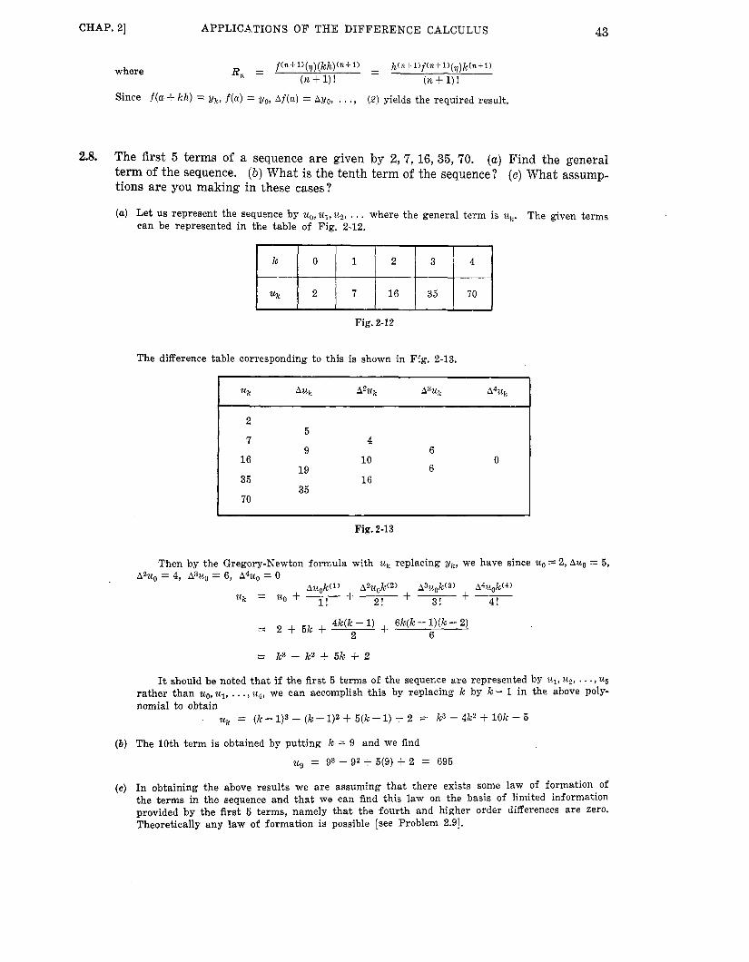
CHAP. 21 APPLICATIONS O F T H E DIFFERENCE CALCULUS
k
uk
43
0 1 2 3 4
2 7 16 35 70
where
Since f ( a + kh) = gk, f(a) = yo, Af(a) = Avo, . . ., ( 2 ) yields the required result.
2.8. The first 5 terms of a sequence are given by 2,7,16,35,70. (a) Find the general term of the sequence. ( b ) What is the tenth term of the sequence? (c) What assump- tions are you making in these cases?
(a) Let us represent the sequence by uo,u1,u2, . . . where the general term is uk. The given terms can be represented in the table of Fig. 2-12.
Fig. 2-12
The difference table corresponding to this is shown in Fig. 2-13. * 16
35
70
9
19
35
10
16
6
6 0
I
Fig. 2-13
Then by the Gregory-Newton formula with uk replacing yk, we have since uo = 2, Auo = 5, A2uO = 4, A3u0 = 6, A4u0 = 0
Auok(l) A2uok(2) A3uOk(3) A4uok(*4) +-+- +- 3 ! 4 ! 2! uk = u0 + - l!
4k(k - 1) + 6k(k - l ) (k - 2) 6 2 + 5 k + - 2
= k3 - k2 + 6k + 2 It should be noted tha t if the first 5 terms of the sequence a r e represented by ul, u2, . . . , u5
ra ther than uo,ul, . . .,u4, we can accomplish this by replacing k by k - 1 in the above poly- nomial to obtain
Uk = (k - 1)s - (k - 1)2 + 5(k - I) -I- 2 = k3 - 4k2 + 10k - 5
( b ) The 10th term i s obtained by putting k = 9 and we find
ug = g3 - 92 + 5(9) + 2 = 695
(c) In obtaining the above results we a r e assuming tha t there exists some law of formation of the terms in the sequence and t h a t we can find this law on the basis of limited information provided by the first 6 terms, namely t h a t the fourth and higher order differences a re zero. Theoretically any law of formation is possible [see Problem 2.91.
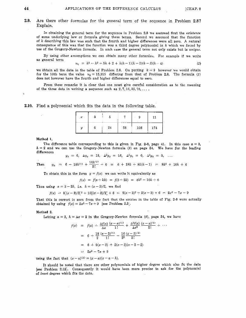
44 APPLICATIONS O F T H E DIFFERENCE CALCULUS [CHAP. 2
2.9. Are there other formulas fo r the general term of the sequence in Problem 2.8? Explain.
In obtaining the general term for the sequence in Problem 2.8 we assumed first the existence of some underlying law o r formula giving these terms. Second we assumed t h a t the function of k describing this law was such tha t the fourth and higher differences were all zero. A natural consequence of this was tha t the function was a third degree polynomial in k which we found by use of the Gregory-Newton formula. In such case the general term not only exists but is unique.
By using other assumptions we can obtain many other formulas. For example if we write
(1 1 as general term
uk = k3 - k2 + 5k + 2 + k ( k - l ) (k - 2) (k - 3 ) ( k - 4)
we obtain all the data in the table of Problem 2.8. On putting k = 9 however we would obtain for the 10th term the value ug = 15,815 differing from tha t of Problem 2.8. The formula (1) does not however have the fourth and higher differences equal to zero.
of the three dots in writing a sequence such as 2 ,7 ,16 ,35 ,70 , . . . . From these remarks i t is clear t h a t one must give careful consideration as to the meaning
).
2.10. Find a polynomial which fits the data in the following table.
24 58
Method 1.
h = 2 and we can use the Gregory-Newton formula (8) on page 34. differences
The difference table corresponding to this is given in Fig. 2-8, page 41. In this case a = 3, We have for the leading
yo = 6, Avo = 18, A'yo = 16, A3y0 = 0, A4yo = 0, . . .
Then yk = 6 + 18k(l) + 16k(2) + 0 = 6 + 18k + 8k(k-1) = 8k2 + 10k + 6
To obtain this in the form y = f(x) we can write i t equivalently as
f ( x ) = f ( a + k h ) = f ( 3 + 2 k ) = 8k2 + 10k + 6
Thus using x = 3 + 2k, i.e. k = (x - 3)/2, we find
f(x) = 8 [ ( x - 3)/2]2 + lo[($ - 3)/2] + 6 = Z(X - 3)2 + 5 ( ~ - 3) + 6 = 2x2 - 7x + 9
That this is correct is seen from the fact that the entries in the table of Fig. 2-8 were actually obtained by using f ( x ) = 2x2 - 7x + 9 [see Problem 2.31.
Method 2. Letting a = 3, h = Ax = 2 in the Gregory-Newton formula (6), page 34, we have
=
= 2x2- 72 + 9
using the fact tha t (x - a)(2) = (x - a)(% - a - h).
[see Problem 2.121. of least degree which fits the data.
6 + 9 ( x - 3 ) + 2 ( 2 - 3 ) ( ~ - 3 - 2 )
It should be noted t h a t there a r e other polynomials of higher degree which also fit the data Consequently i t would have been more precise to ask f o r the polynomial

CHAP. 21 APPLICATIONS O F T H E DIFFERENCE CALCULUS 45
INTERPOLATION AND EXTRAPOLATION 2.11. Use the table of Problem 2.10 to find the value of y corresponding to (a) x=8,
(b) x = 5.5, (c) x = 15, (d) x = 0. ( e ) What assumptions are you making in these cases?
2.12.
Method 1. From Method 1 of Problem 2.10 we have yk = 8k2 + 10k + 6. To find the value of k corres-
ponding to x = 8 we use x = a + k h with a = 3, h = 2 to obtain k = (x - a ) / h = ( 8 - 3)/2 = 2.6. Thus the required value of y corresponding to x = 8 is
~ 2 . 5 = 8(2.5)’ + lO(2.5) + 6 = 81 In a similar manner the values of k corresponding t o x = 5.5, x = 15, x = 0 are (6.6 - 3)/2, (15 - 3)/2, (0 - 3)/2 or 1.25, 6, -1.5 respectively. Then the required values of y corresponding to x = 5.5, 15 and 0 a r e respectively
~ 1 . 2 5 = 8(1.25)2 + lO(1.25) + 6 = 31, 8(6)2 + lO(6) 6 = 354
1/ -1 .5 = 8(-1.5)2 + 10(-1.5) + 6 = 9
Method 2. From either Method 1 or Method 2 of Problem 2.10 we have
y = f(x) = 2x2 - 7% + 9
Then the required values a r e f(8) = 2(8)2 - 7(8) + 9 = 81
f(5.5) = 2(5.5)2 - 7(5.5) + 9 = 31
f(15) = 2(15)2 - “(15) + 9 = 354
f(0) = 2(0)2 - 7(0) + 9 = 9
Note t h a t in par ts (a) and ( b ) we are interpolating, i.e. finding values within the table, while in par ts (c) and ( d ) we a r e ex trapola t ing , i.e. finding values outside the table.
(e) In using the method we are assuming t h a t there ex is t s some underlying law which the data follows and tha t we can find this law on the basis of the limited information supplied in the
* table which suggests tha t all third and higher differences a r e actually zero so t h a t the data is fitted by a polynomial of second degree. It is possible however t h a t even if a n underlying law exists, i t is not unique. The analogy with finding general terms of sequences or series as discussed in Problem 2.9 is apparent.
(a) Give an example of a polynomial of degree higher than two which fits the data of Problem 2.3. ( b ) Discuss the relationship of this to problems of interpolation and extrapolation.
(a) One example of a polynomial fitting the data of Problem 2.3 is obtained by using
F ( x ) = 2x2 - 7 x + 9 + (x - 3)(x - 5)(x - 7)(x - 9)(x - 11) (1 )
which is a polynomial of degree 5. table or equivalently those obtained from f ( z ) = 2x2 - 7x + 9. For x = 3,5 ,7 ,9 ,11 the values agree with those of the
Other examples can easily be made up, for example the polynomial of degree 11 given by
F, ($1 = 2x2 - 7% + 9 + 3(x - 3)2(x - 5)(x - 7)4(2 - 9)(2 - 11)3
F,(x) = 2x2 - 7x + 9 + (x - 3)(x - 5)(x - 7)(x - 9)(x - 1l)e-5
(2)
(4 F o r a n example of a function which fits the data but is not a polynomial we can consider
( b ) Since there a r e many examples of functions which fit the data, i t i s clear t h a t any interpola- tion formula based on data f rom a table will not be unique. Thus for example if we put x = 8 in (1) of par t ( a ) , we find the value corresponding to i t is 126 ra ther than 81 as in Problem 2.11.
Uniqueness is obtained only when we restrict ourselves in some way as for example requiring a polynomial of smallest degree which fits the data.

46 APPLICATIONS O F THE DIFFERENCE CALCULUS [CHAP. 2
X
sin x
2.13. The table of Fig. 2-14 gives the values of sinx from x = 25" t o x = 30" in steps of 1". (a) Using interpolation find sin 28' 24' and ( b ) compare with the exact value.
25" 26" 27" 28O 29 " 30"
0.42262 0.43837 0.45399 0.46947 0.48481 0.50000
To avoid decimals consider f(z) = lo5 sin x and let x = a+ kh where a = 25" and h = lo. Then we can write v k = f ( a + kh) = 105 sin (25O + k lo). The difference table is given in Fig. 2-15. In this table k = 0 corresponds to x = 25", k = 1 to 26O, etc.
1 0
~1 I
2
3
4
5
42,262
43,837
45,399
46,947
48,481
50,000
1,575
1,562
1,548
1,534
1,519
-13 -1
-14
-14
-15
0
-1
Fig. 2-15
It should be noted that the third differences are very small in comparison with the 1/k and for all practical purposes can be taken as zero.
When x = 28'24' = 28.4O, we have k = (28.4' - 25')/1' = 3.4. Thus by the Gregory-Newton formula
y3,4 = 105 sin (28' 24')
(-13)(3.4)(3.4 - 1) + . . . 2! = 42,262 + (1,575)(3.4) +
= 47,564
This yields a value of sin 28O 24' = 0.47564. For an estimate of the error see Problem 2.14.
( b ) The exact value t o 5 decimal places is 0.47562. Thus the absolute error made is 0.00002 and the percent error is 0.004%.
2.14. Estimate the error term in Problem 2.13. The error is given by the remainder (7), page 34, with n = 2
h3f"'(q) k(3) 3! R2 =
To evaluate this note that in formulas of calculus involving trigonometric must be expressed in radians rather than degrees. This is accomplished by radians. If x is in radians we have
f(x) = 105 sinx, f'(x) = 105 cosx, f " (z) = -105 sinx, f " ' ( x ) =
so that (1) becomes (COS 7)(3.4)(3.4 - 1)(3.4 - 2)
R, = -105(~) 3!
(1 )
functions, angles using lo = 1;/180
-10s cos x

47 CHAP. 21 APPLICATIONS O F T H E DIFFERENCE CALCULUS
Since the largest value of cos q is dl - sin225O = 0.90631 we see from (2) that R, = -1 approximately, i.e. the best value we can get for sin28O24' is 0.47563. The fact tha t this is still not correct is due to rounding errors in the given table.
CENTRAL DIFFERENCE TABLES AND INTERPOLATION FORMULAS
2.15. (a) Construct a central difference table corresponding to the data of Problem 2.13 by choosing a = 28'. (b) Use Stirling's interpolation formula to work Problem 2.13 and ( c ) compare with the exact value and the value obtained from the Gregory- Newton formula.
(a ) The central difference table is shown in Fig. 2-16.
-3
-2
-1
0
1
2
~~
42,262
43,837 -13
45,399 -14
1,575
1,562 -1
1.548 0 46.947 ~,~ ~-
1,534
1,519 48,481
50,000
-14
-15 -1
Fig. 2-16
( b ) Here k = 0 corresponds to 28O, k = 1 corresponds to 29O, k = -1 corresponds to 2 6 O , etc. The value of k corresponding to 28.4O is k = (28.4O -28')/1' = 0.4.
From the table we see tha t
YO = 46,947, A u - 1 = 1,548, Ayo = 1,534, A'y-1 = -14, A 3 ~ - 2 = -1, A3y-1 = 0
Then by Stirling's formula
yo,4 = lo5 sin (28'24')
= 47,662
Thus sin 28'24' = 0.47562.
(c) The result obtained in ( b ) is correct to 5 decimal places. The additional accuracy of Stir- ling's formula over the Gregory-Newton formula is explained by the fact that 28O.24' = 28.4' occurs in the central par t of the table. Thus the Stirling formula, which uses the differences near the center, is expected to be more accurate than the Gregory-Newton formula, which uses differences near the beginning of the table.

48 APPLICATIONS O F T H E DIFFERENCE CALCULUS [CHAP. 2
2.16. (a) Explain why you might expect Bessel's interpolation formula to give a better approximation to sin 28"24' than Stirling's formula. ( b ) Can you confirm your expectation given in part (a)?
(a) Since the differences used in Bessel's interpolation formula lie to one side of the center i t might be expected tha t since 28.4O lies to the same side, a better approximation would be obtained.
( b ) From the table of Fig. 2-16,
yo = 46,947, ~1 = 48,481, hyo = 1,534, Azy-1 = -14, A21Jo = -15
Thus Bessel's interpolation f o r m u b gives
(0.4)(--0.6) + . . . or yo,4 = +(46,947 + 48,481) + 1,534[+(0.4 - 0.6)] + &(-14 - 15) L 2 1 = 47,562
Thus we obtain sin 28O24' = 0.47562. Although Bessel's formula might have been expected to give a better approximation than Stirling's formula we cannot confirm the expectation in this case since the result obtained from Stirling's formula is already accurate to 5 decimal places.
2.17. Derive the Gregory-Newton backward difference formula by (a) using symbolic operator methods, ( b ) using any other method.
(a) We have since E - A = 1 = (&)210 k =
(1 - AE-l)--kyo
(-k)(-k - l)(-AE-1)2 + (-k)(-k - 1)(-k - Z)(-AE-1)3 2! 3! = [l + ( -k ) ( -AE-I ) +
where we have used the binomial theorem.
( b ) Assume yk = A , + A , k ( l ) + Az(k + 1)(2) + A 3 ( k + 2)(3) + 9 * * + A,(k + n - l ) ( n )
= A , + 2 A 2 ( k + l ) ( l ) + 3 A 3 ( k + 2)tz) + - - - + nA,(k+ n- l ) ( n - l ) Then Ayk
A z u k - - 2A2 + 6A3(k + 2)(1) + . + n(n - 1)A,(k + n - 1)'n-Z)
............................................... . . . . . . . . . . . . . . I . . ,
A"yk = % ! A ,
Putt ing k = 0 in the expression for yk, k = -1 in Auk, k = -2 in A2yk, . . . we find

CHAP. 21 APPLICATIONS O F T H E DIFFERENCE CALCULUS 49
2.18. Derive the Gauss interpolation formulas from the Gregory-Newton formula. The Gregory-Newton formula is
k(1) k'2) k(3) yk = yo Avo- + A2yy,- + A 3 y - + . . *
l! 2 ! O 3!
Now from the generalized difference table of Fig. 2-4, page 35, we have
A2yo - A 2 y - 1 = A3Y-1 or A2yo = A 2 y - l 4- A3Y-1
Similarly, A3yo-A3$ / - l = A4y-1, A 4 u - 1 - A 4 2 / - 2 = A5Y-2
from which A3y0 = A32/-1 + A 4 y V l = A 3 y - 1 + A4yP2 + A5y-2
Then by substituting in the Gregory-Newton formula we find
The second Gauss formula can be derived in a similar manner [see Problem 2. )4].
2.19. Derive Stirling's interpolation formula. From the Gauss formulas we have
Then taking the arithmetic mean of these two results we have
2.20. Show how to express the Gregory-Newton backward difference interpolation formula in terms of the backward difference operator V.
By Problems 1.39(u), page 25, and 1.93, page 30, we have
V = A E - 1 , V2 = A 2 E - 2 , ..., V n = A n E - "
Thus A n E - n f ( u ) = V n f ( a ) n = 1 ,2 ,3 , . . .
or equivalently A n E - n y o == V n y o
Using this in (8), page 34, i t becomes
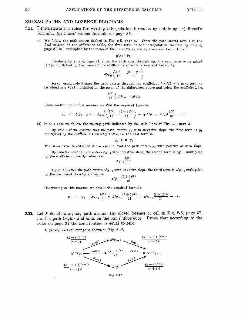
50 APPLICATIONS O F T H E DIFFERENCE CALCULUS [CHAP. 2
ZIG-ZAG PATHS AND LOZENGE DIAGRAMS 2.21. Demonstrate the rules fo r writing interpolation formulas by obtaining (a) Bessel's
formula, ( b ) Gauss' second formula on page 36.
We follow the path shown dashed in Fig. 2-5, page 37. Since the path starts with 1 in the first column of the difference table, the first term of the interpolation formula by rule 5 , page 37, is 1 multiplied by the mean of the numbers yo and yl above and below 1, i.e.
&(Yo + Y l )
Similarly by rule 4, page 37, since the path goes through Ago the next term to be added is Ay, multiplied by the mean of the coefficients directly above and below, i.e.
Again using rule 5 since the path passes through the coefficient k ( 2 ) / 2 ! , the next term t o be added is k ( 2 ) / 2 ! multiplied by the mean of the differences above and below the coefficient, i.e.
Thus continuing in this manner we find the required formula
In this case we follow the zig-zag path indicated by the solid lines of Fig. 2-5, page 37.
multiplied by the coefficient 1 directly above, i.e. the first term is By rule 2 if we assume tha t the path enters yo with negative slope, the first term is yo
Y o ' l = Yo The same term is obtained if we assume tha t the path enters yo with positive o r zero slope.
By rule 3 since the path enters Ay-l with positive slope, the second term is Ay-1 multiplied k( l ) by the coefficient directly below, i.e.
Ay-1-
By rule 2 since the path enters A2yP1 with negative slope, the third term is A2y-1 multiplied by the coefficient directly above, i.e.
( k 4- 1)(2) A ' Y - 1 ~ 2 !
Continuing in this manner we obtain the required formula
2.22. Let P denote a zig-zag path around any closed lozenge or cell in Fig. 2-5, page 37, i.e. the path begins and ends on the same difference. Prove that according to the rules on page 37 the contribution is equal to zero.
A general cell or lozenge is shown in Fig. 2-17.
Fig. 2-17

CHAP. 21 APPLICATIONS O F T H E DIFFERENCE CALCULUS 51
By rule 6 a reversal of path changes the sign of the corresponding term added, Thus we need only show tha t the contributions corresponding to the three paths from An-'y,. to Antly,.-l in Fig. 2-17 a r e all equal.
Now if path 1 is chosen the contribution is
Similarly if paths 2 and 3 are chosen the contributions are respectively
From (1) and (3) we see tha t
( k - r + l ) ( n + l ) ( k - r ) ( n + l ) - (n + 1) ! (n + 1 ) !
(k - ~ ) ( n ) c1 - c3 = (An?./,.-l-Any,.) + An+l?./,.-l n!
= o so t h a t C1 = C3. Also we note t h a t the mean of C1 and C3 is
Thus C, = C p = C3 and the required result is proved.
2.23. Prove that the sum of the contributions around any closed zig-zag path in the lozenge diagram is zero.
path encloses 3 cells I, 11, 111. We shall prove the result for a typical closed path such as JKLMNPQRJ in Fig. 2-18. This
L
Fig. 2-18
If we denote the contribution corresponding to path J K , for example, by C j K and the total contribution around cell I, for example, by CI, then
CI + CII + CHI = ( cJK + C X N + Ch'R + C R J )
+ ( C K L + C L M + CMN + Ch7K)
+ (CRN + C N P + CPQ + CQR) = CJK + CKL + CLM + CMN + CNP + CPQ + CQR + CRJ
+ ( C K N + CNK) + ( C R N + CNR)
= CJKLMNPQRJ since CKN = -CNK and CRN = -CNR. lows tha t CJKLMNPQRJ = 0.
Thus since C, = 0, CIr = 0, = 0 by Problem 2.22, i t fol-

52 APPLICATIONS O F THE DIFFERENCE CALCULUS [CHAP. 2
224. Prove that if two zig-zag paths end at the same place in the lozenge diagram then the interpolation formulas corresponding to them are identical.
two paths end a t the same place but begin at different places. Consider for example the two zig-zag paths indicated dashed and solid in Fig. 2-19. These
( k - ?.)(I)
yr \ l ! \ \
Fig. 2-19
The total contribution to the interpolation formula corresponding to the dashed path is given by
when R is the remaining par t of the formula.
Similarly the total contribution to the interpolation formula corresponding to the solid path is
+ R ( 2 ) ( k - v - 1)(1)
- Aur 1 !
Note t h a t the minus signs in (1) and ( 2 ) are used because of rule 6, page 37.
To show tha t the results (1) and ( 2 ) are actually equal we need only show tha t their difference is zero. We find this difference to be
Since yrt l = yr +Aur, (3) can be written
so t h a t the required result is proved.
2.25. Prove the validity of all the interpolation formulas on page 36.
they a r e all valid if we can prove just one of them. namely the Gregory-Newton formula on page 36.
Since all the formulas can be obtained from any one of them, i t follows by Problem 2.24 that However we have already proved one of them,
Note t h a t Problems 2.18 and 2.19 illustrate how some of these formulas can be obtained from
This proves tha t all of them are valid.
the Gregory-Newton formula.
LAGRANGE'S INTERPOLATION FORMULA 2.26. Prove Lagrange's interpolation formula on page 38.
page 32, we can fit the data by a polynomial of degree p . Since there a r e p + 1 values of g corresponding to p + 1 values of x in the table of Fig. 2-1 on
Choose this polynomial to be
u = ao(x - xl)(x - x2). * * (x - xp) + al (z - x o ) ( 5 - x2) ' ' * (x - xp) + * * * + Up(% - xo)(x - X1)' * '(X - x p - J

CHAP. 21 APPLICATIONS O F T H E DIFFERENCE CALCULUS 53
Then putting x = xo, y = yo we have Yo yo = a o ( x o - x , ) ( x o - ~ 2 ) ~ ~ ~ ( ~ O - ~ p ) or a. =
(xo - x1)(xo - x 2 ) ' * * (xo - x p ) Similarly putting x = xl, y = y1 we find
Y1 y1 = a l ( x l - ~ O ) ( ~ 1 - ~ 2 ) ~ ~ ~ ( ~ 1 - ~ p ) or al = ( X I - xo)(x1- xz). * '(xl- x p )
with corresponding values for a2, a3. . . , , up, obtain Lagrange's formula.
Putting these values in the assumed polynomial we
2.27. (a) Work Problem 2.10 by using Lagrange's formula and thus ( b ) solve Problem 2.11. (a) Substituting the values from the table of Fig. 2-13 into Lagrange's formula we obtain
(x - 5)(x - 7 ) ( 2 - 9)(x - 11) (x - 3)(x - 7)(x - 9)(x - 11) (3 - 5)(3 - 7)(3 - 9)(3 - 11) + 24 (5 - 3)(5 - 7)(5 - 9)(5 - 11) Y =
(x - 3)(x -- 5)(x - 9)(x - 11) (x - 3)(x - 5)(x - 7)(x - 11) + 58 (7 - 3)(7 - 5)(7 - 9)(7 - 11) + log (9 - 3)(9 - 5)(9 - 7)(9 - 11)
(x - 3)(x - 5)(x - 7)(x - 9) + 174 (11 - 3)(11 - 5)(11- 7)(11- 9)
Performing the algebra we find y = 2x2 - 7x + 9 which is a polynomial of degree two and not four as we might have expected.
( b ) The values of y for 2 = 8,5.5,15,0 can be obtained by substituting in the Lagrange inter- polation formula of par t (a).
TABLES WITH MISSING ENTRIES 2.28. Find the value of u3 missing in the following table.
Fig. 2-20
Method 1.
(k,u,) which a r e known we would be able to fit a polynomial of degree 3. t h a t the fourth differences a re zero, i.e. A4u0 = 0.
(E - l)4u0 = (E4 - 4E3 + 6Ez - 4 E + l )u0 = 0
In this problem we cannot construct a difference table. However from the four pairs of values This leads us to assume
Thus we have
which becomes ~q - 4 ~ 3 + 6 ~ 2 - 4Ul + uo = 0
Using the values from the table we then have
47 - 4u3 + 6(15) - 4(8) + 3 = 0 or u3 = 27
Method 2.
of degree 3 which involves 4 unknown coefficients. Since there a r e 4 values of k for which uk i s known, we can fit the data by a polynomial
Let us therefore assume t h a t
u k = A0k3 + Alk2 + A,k + A ,
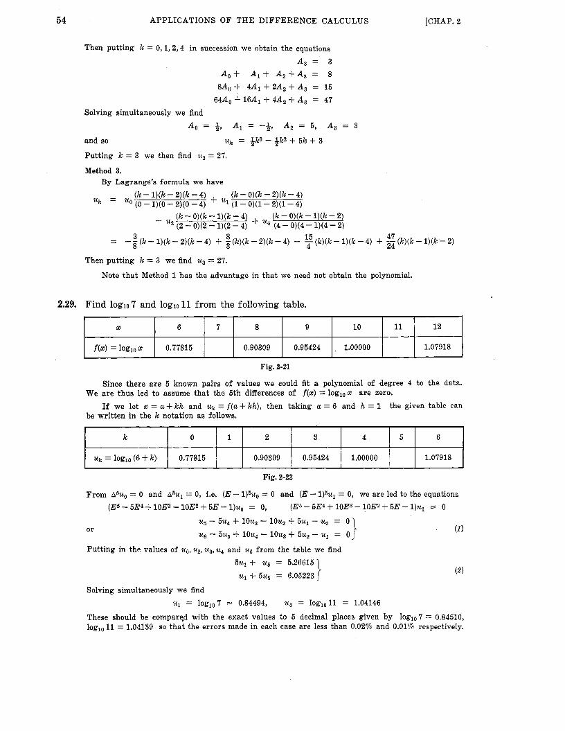
54 APPLICATIONS OF THE DIFFERENCE CALCULUS
5 6 7 8 9
f ( x ) = loglo x 0.77815 0.90309 0.95424
[CHAP. 2
10 11 12
~ 1.00000 1.07918
Then putting k = 0, 1 ,2 ,4 in succession we obtain the equations
A3 = 3 A , + A I + A , + A 3 = 8
8Ao+ 4 A , + 2 A , + A 3 = 15
64A, + 16A1 + 4Az + A, = 47 Solving simultaneously we find
A, = 1, A, = -1 2, Az = 5, A3 = 3
Uk = 8k3 - Qkz + 5k f 3 a
and so
Putting k = 3 we then find u3 = 27.
Method 3. By Lagrange's formula we have
k
Uk = log10 (6 + k)
(k - l ) (k - 2)(k - 4) (k - O)(k - 2)(k - 4) uo (0 - 1)(0 - 2)(0 - 4) + u1 (1 - 0)(1- 2)(1- 4) uk =
0 1 2 3 4 5 6
0.77815 I 0.90309 0.95424 1.00000 1.07918
(k - O)(k - l ) (k - 4) + u2 (2 - 0)(2 - 1)(2 - 4)
(k - O)(k - l ) ( k - 2) u4 (4 - 0)(4 - 1)(4 - 2)
3 8 15 47 = -8 (k - l ) (k - 2)(k - 4) + 3 (k)(k- 2)(k- 4) - ;?- (k)(k - l ) (k - 4) + ;i;i (k)(k - l)(k'- 2)
Then putting k = 3 we find u3 = 27.
Note that Method 1 has the advantage in that we need not obtain the polynomial.
Fig. 2-22
From A5u0 = 0 and A5u, = 0, i.e. (E - l ) 5 u ~ = 0 and (E - l ) b , = 0, we are led to the equations
(E5 - 5E4 + lOE3 - 10E2 + 5E - l ) ~ , = 0, (E5 - 5E4 + lOE3 - 10E2 + 5 E - 1)ul = 0
or
Putting in the values of uo, u2, us, u4 and u6 from the table we find
5U, 4- ~5 = 5.26615
U , + 5 ~ 5 = 6.05223
Solving simultaneously we find U, = loglo7 = 0.84494, ~5 = log10 11 = 1.04146
These should be comparcd with the exact values to 5 decimal places given by loglo 7 = 0.84510, loglo 11 = 1.04139 so that the errors made in each case are less than 0.02% and 0.01% respectively.
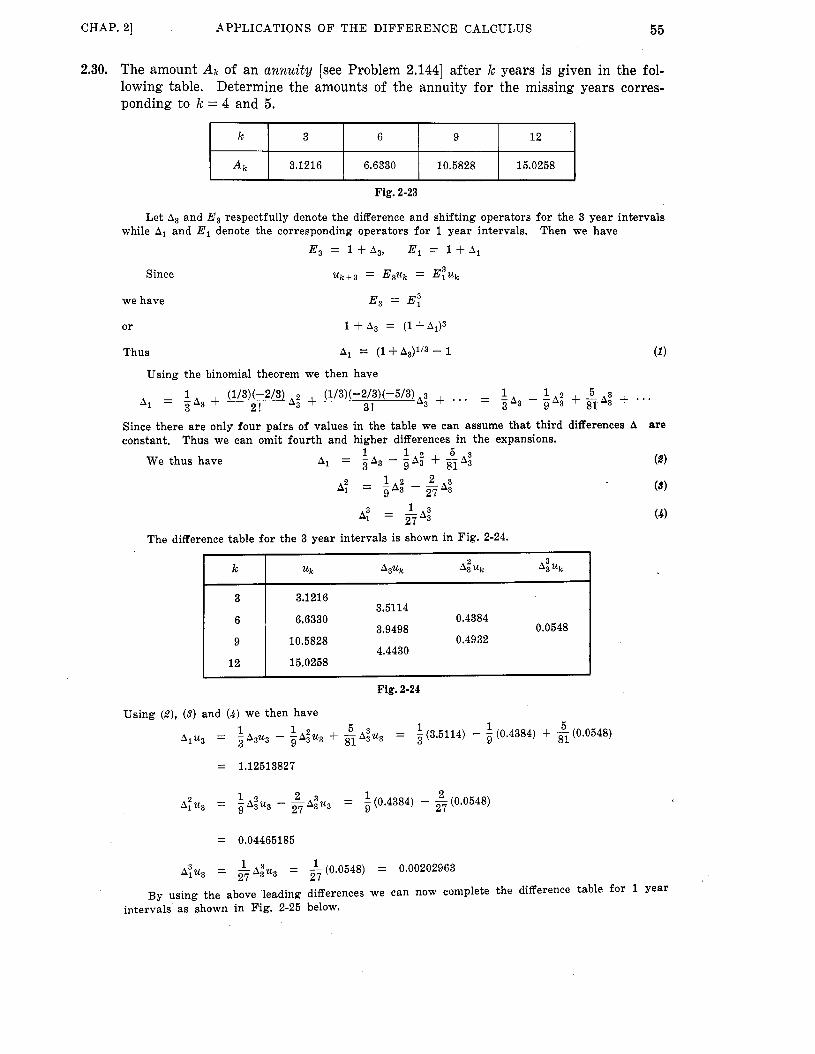
CHAP. 21 APPLICATIONS OF THE DIFFERENCE CALCULUS 55
k
2.30. The amount Ak of an annuity [see Problem 2.1441 after k years is given in the fol- lowing table. Determine the amounts of the annuity for the missing years corres- ponding to k = 4 and 5.
3 6 9 12
A k I 3.1216 6.6330 10.5828 15.0258
Fig. 2-23
Let A3 and E3 respectfully denote the difference and shifting operators for the 3 year intervals while A1 and E l denote the corresponding operators for 1 year intervals. Then we have
E3 = 1 + A , , El = 1 + A 1
U k + 3 = E 3 U k = E ; U k Since
we have E3 = EY
or 1 'r A3 = ( I + A I ) ~
Thus A1 = (1 +A3)1'3 - 1 (1 1 Using the binomial theorem we then have
= 1 + + (1/3)(-2/3)(-5/3)~: + . . . = 1 A3 - s A i 1 + sl 5 A: + . 3!
Thus we can omit fourth and higher differences in the expansions. Since there are only four pairs of values in the table we can assume that third differences A constant,
are
(8) 1 1 5
9 A, = ? A 3 - -A; 4- EA: We thus have
k uk A3Uk uk A; uk
I I I 3.1216
3.5114 6.6330 0.4384
3.9498 0.0548 10.5828 0.4932
4.4430
Using (Z), (3) and ( 4 ) we then have 1 5 1 1 5
Alu3 = l A 3 u 3 3 - -Aiu3 9 + a Aiu3 = -(3.5114) 3 - 9 (0.4384) + (0.0548)
= 1.12513827
2 1 2 A : U ~ = $Aiu3 - -A:u3 = -(0.4384) 9 - ~ ( 0 . 0 5 4 8 ) 27
= 0.04465185
1 1 ~ : u 3 = - A ; u 3 27 = -(0.0548) 27 = 0.00202963
By using the above leading differences we can now complete the difference table for 1 year intervals as shown in Fig. 2-25 below.
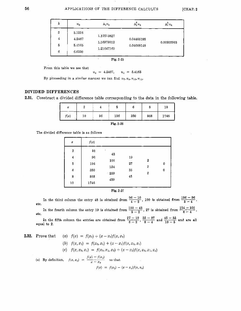
56
k
3
4
5
6
APPLICATIONS O F THE DIFFERENCE CALCULUS [CHAP. 2
u k * l U k A? Uk 4 U k
3.1216
4.2467 0.04465185
5.4165 0.04668148
6.6330
1.12513827
1.16979012 0.00202963
1.21647160
- X 2 4 5 6 8 10
f(x) , 10 96 196 350 868 1746
From this table we see tha t uq = 4.2467, U S = 5.4165
By proceeding in a similar manner we can find u,, us, ul0, ull .
1 2 1 10
4
5
6
8
10
96
196
350
868
1746
43
100
154
259
439
19
27
35
45
0
0
Fig. 2-27
96 - 10 196 - 96 , 100 is obtained from - In the third column the entry 43 is obtained from 4--2 5 - 4 , In the fourth column the entry 19 is obtained from ____ loo - 43 , 27 is obtained from 154 - - 100 ,
etc.
etc. 5 - 2
45 - 35 and a r e all In the fifth column the entries a r e obtained from m, 8-4 and ~ 10 - 5 2 7 - 19 35 - 2 7
equal to 2.
2.32. Prove that (a) f(x) = f (xo) + (x - xo)f(x, $0)
( b ) f(x, xo) = f (x0, Xl) -t (x - % l ) f ( X , Xot X l )
(c) f(x, xo, X l ) = f ( x0 , x1, xz) + (X - xz ) f ( x , xo, x1, xz) f(x) - mo) so that
(a) By definition, f ( x , x 0 ) = x - xo

CHAP. 21 APPLICATIONS O F T H E DIFFERENCE CALCULUS 57
2.34. Prove Newton's divided difference interpolation formula f(x) = f (x0) + (x - xo)f(lro, X l ) + (x - xo)(x - x1)f(xo, x1, xz)
R(x) = (x - xo)(x - X l ) * * * (x - xn) f (x , xo, x1, . . . ' x,) + a + (x - xo) * ' (x - xn-l)f(xo, . . . , x,) + R(x)
where We shall use the principle of mathematical induction. Assume tha t the formula is t rue for
n = lc, i.e. f(x) = f(x0) + (5 - xo)f(xo, + * ' ' + (x - %O) ' * * (x - ~ k - l l ) f ( x O , . . ., Xk)
+ (x - xO)(x - x1) * * * (x - xk)f(x, x0, x1, * * * , zk) (1)
Now by definition as in Problem 2.32 we have
(2)
($1
f(x, x0, . * * t x k ) - f(x0, 51, * * * , Z k + l )
x - x k + l f(x, $0, %1t * * * , $k+ 1) =
so tha t
Using this in (1) we find
f(x, xo, xi, . . . , % k ) = f ( x0 , $1, . . . , x k f 1) + (x - %k + x0, %1, * * * f xk t 1)
f(x) = f(%o) + (x - %o)f(xo, X i ) + ' * + (x - 2,) ' ' ' (x - % k ) f ( Z o , t zk + 1)
-k (x - xo)(x - El) ' ' '(x - x k t l ) f ( x , xot $1, * * * t z k + l )
Thus assuming tha t it is t rue for n = k we have proved it t rue for n = k + 1. true for n = 1 [see Problem 2.321, i t i s t rue for n = 2 positive integers.
But since it is an& so on for all and thus for n = 3
2.35. Prove that the remainder in Problem 2.34 can be written as fcn+Y?) (n + 1) ! R(x) = (x-xXo)(X-xXI)...(X--Xn)
where 7 is a number between the smallest and largest of the values x, xo, xi, . . . , Xn. (1 )
By Problem 2.34 the remainder is R(z) = (x - xo)(x - x1) * . (5 - x,) f (x , xo,x1, . . . , x,)

60 APPLICATIONS O F THE DIFFERENCE CALCULUS [CHAP. 2
( c ) Since the values of z are equally spaced we can use the Gregory-Newton formula to find an interpolating formula for f(s). As in Problem 2.11 we find f(x) = 2x2 - 7x + 9.
If f(x) = 100, i.e. 2x2 - 72 + 9 = 100, then 2x2 - 72 - 91 = 0 and by solving this equation we find
6 7 ‘-c - 7 27.8747
4 4 - x =
Since only the positive square root is significant for our purposes, we use i t to find x = 8.718. This can in fact be taken as the true value of x since the table of Problem 2.10 was actually constructed by using the function f(x) = 2x2 - 7% + 9.
2.39. Work Problem 2.37 by using inverse interpolation involving Lagrange’s formula. We use the table of Fig. 2-28, page 58. Then by Lagrange’s interpolation formula we have
(y + 1.0390)(16 - 0.0480)(~ - 1.2670)(~ - 2.6240) 2*o (-2.0000 + 1.0390)(-2.0000 - 0.0480)(-2.0000 - 1.2670)(-2.0000 - 2.6240) x =
(y + 2.0000)(~ - 0.0480)(~ - 1.2670)(~ - 2.6240) + 2*1 (-1.0390 + 2.0000)(-1.0390 - 0.0480)(--1.0390 - 1.2670)(--1.0390 - 2.6240)
(y + 2.0000)(~ + 1.0390)(~ - 1.2670)(1/ - 2.6240) + 2*2 (0.0480 + 2.0000)(0.0480 + 1.0390)(0.0480 - 1.2670)(0.0480 - 2.6240)
(y + 2.0000)(~ + 1.0390)(~ - 0.0480)(~ - 2.6240) + 2*3 (1.2670 + 2.0000)(1.2670 + 1.0390)(1.2670 - 0.0480)(1.2670 - 2.6240)
(y + 2.0000)(~ + 1.0390)(~ - 0.0480)(2/ - 1.2670) + 2*4 (2.6240 + 2.0000)(2.6240 + 1.0390)(2.6240 - 0.0480)(2.6240 - 1.2670)
Since the required value of x is the one for which y = 0, above result x = 2.19583 in agreement with that of Problem 2.37.
we obtain on putting y = 0 in the
APPROXIMATE DIFFERENTIATION 2.40. Establish equation (16), page 39, (a) by symbolic operator methods and ( b ) by using
the Gregory-Newton formula.
(a) In using symbolic operator methods we proceed formally. We start with
ehD = 1 + A
Taking logarithms this yields [equation ( 4 4 , page 81.
Then using the formal Taylor series on page 8 we find
1 A2 A3 A4 D = ~ I n ( 1 - l - A ) = h A - - + - - - + . . - q 2 3 4
( b ) By the Gregory-Newton formula,
A2f (a) k(k - 1)
f (a+ kh) = f(a) + k A f ( a ) + A4f(a) * *
k(k - l ) ( k - 2)(k - 3) Asf(a) + 4!
k(k - l ) (k - 2) 3! +
Then differentiating with respect to k,
A3f (4 2k - 1 3k2 - 6k + 2 hf’(a+ kh) = Af(a) + --g- A2f(a) + 3!
~ A4f(a) 4- * * 4k3 - 18k2 + 22k - 6
4! +

CHAP. 21 APPLICATIONS OF
X
f ( z )
THE DIFFERENCE CALCULUS
0.25 0.35 . 0.45 0.55 0.65 0.75
0.24740 0.34290 0.43497 0.52269 0.60518 0.68164
6 1
Since !(a) is arbitrary we have A2 A3 A4 D = - A - - +- - -+ . . .
h l ( 2 3 4
If we take into account the remainder term in the Gregory-Newton formula, then we can find a corresponding remainder term for the derivative.
We consider the difference table for lOjf(x) so as to avoid decimals. This table is as follows. The difference columns are headed A, A2, . . . in place of 105Af(x), 105A2f(x), . . . f o r brevity.
105f(4 A A2 A3 A4 A5
24,740 9550
34,290 -343
43,497 9207 -92
-435 4 8772 -88
52,269 -523 8 8249 -80
60,518 -603 7646
68,164
4
Fig. 2-31
Using the formula of Problem 2.40 we have
A2 A3 A4 ’ D[105f(x)] =
(A - + 3 - 7 + and neglecting differences of order 5 and higher we find for x = 0.25
or f’(0.25) = 0.96898.
f’(z) = cos x, The table of values are those f o r f ( x ) = sinx where x is in radians. From this we see that
By way of comparison the true value is f’(0.25) = cos 0.25 = 0.96891.
2.42. Use the table of Fig. 2-31 From Problem 2.40,
so that on squaring we find
to find f” (0 .25 ) .

62 APPLICATIONS O F T H E DIFFERENCE CALCULUS
Year
Population in millions
[CHAP. 2
1930 1940 1950 1960 1970
1.0 1.2 1.6 2.8 5.4
Thus D 2 f ( x ) = L ( A 2 - A 3 + u A 4 + 1 2 ...)f( x) h2
From this i t follows tha t 1 105f”(0.25) = (-343 + 92 + 3.7) = -25,470
or f”(0.25) = -0.25470.
The exact value is f”(0.25) = -sin 0.25 = -0.24740. .
2.43. Referring to the table of Fig. 2-31 find f’(0.40).
From the Gregory-Newton formula we have
A3f(a) + ’ k(k - 1) k(k - l)(k - 2)
3! f(a + kh) = f(a) + kAf(a) + 2! A2f(a) + Differentiation with respect to k yields
4k3 - 18k2 + 22k - 6 4! A3f(a) + + 2k - 1 3k2 - 6k + 2
hf’(a+kh) = Af(a) + + 3!
Letting a = 0.25, h = 0.1 and a + k h = 0.40 so tha t k = 1.5 we find using the difference table of Problem 2.41
105f’(0.40) = - [9550 + (-343) - &(-92) + 0(4)] 1 0.1
f’(0.40) = 0.92108
The t rue value is f’(0.40) = cos 0.40 = 0.92106.
MISCELLANEOUS PROBLEMS 2.44. The population of a particular country during various years is given in the following
table. Obtain an estimate for the population in the year (a) 1980, ( b ) 1955 and (c) 1920.
Fig. 2-32
Let us denote the year by x and the population in millions by P. Since the years given are equidistant i t i s convenient to associate the years 1930, 1940, 1950, 1960, 1970 with the numbers k = 0, 1 , 2 , 3 , 4 respectively. This is equivalent to writing x = a + kh where a = 1930 and h = 10 so tha t
(1 - 1930 10 x = 1930+ 10k o r k =
Using this we can rewrite the given table as follows.
;I Fig. 2-33
The difference table corresponding to this is as follows.

CHAP. 21 APPLICATIONS O F T H E DIFFERENCE CALCULUS
AP A2P A3P
0.6 1.4 I I
I I
Fig. 2-34
63
We shall assume tha t the third differences a re all constant [equal to 0.61 and t..at the fourth differences a r e zero. Then using the Gregory-Newton formula we find
0 2k(2) 0 6k(3) 2! 3!
P = 1.0 + (0.2)k(’) + - + - =
= 1.0 + 0.212 + O.lk(k - 1) + O.lk(k - l)(k - 2)
A ( k 3 - 2k2 + 3k + 10)
(a) From (1) we see t h a t the year 1980 corresponds to k = 5 so tha t
P = &[53-2(5)2+ 3(5)+ 101
Thus we estimate tha t in 1980 the population will be 10 million.
(b) From ( 1 ) we see t h a t the year 1955 corresponds to
1955 - 1930 = 2.5 10 k =
Then P = &[(2.5)3 - 2(2.5)2 + 3(2.5) + 101 = 2.0625
Thus to two significant figures we would estimate tha t the population in 1955 was 2.1 million.
( c ) The value of k corresponding to the year 1920 is from (1)
= -1 1920 - 1930 10
P = &[(-l)3 - 2(-1)2 + 3(-1) + 101 = 0.4
k =
Then
Thus we estimate tha t the population in 1920 was 0.4 million.
,2.45. Suppose that it is necessary to determine some quantity y a t the time when it is a maximum or minimum. Due to error we may not be able to do this exactly. How- ever we observe that at times t1 , t~, t3 near the time for maximum or minimum, the values are given respectively by yl, y ~ , y3. Prove that the time at which the quantity is a maximum or minimum is given by
y1(tz” - t i) + Y2( t i - t l ) + y3(t:: - t i) 2[yl(t2 - t3) f yZ(t3 - tl) + Y3( t l - t2)]
By Lagrange’s formula the value of y at time t is given by
(1 1 ( t - t2)(t - t3) ( t - M t - t3) ( t - tl)(t - t z ) ?dl (tl - M t l - t3) + y2 (t2 - t , ) ( t2 - t3) + y3 (t3 - tl)(t3 - t 2 ) I d =
The maximum or minimum of y occurs where dyldt = 0 [assuming it to be a relative maximum or minimum]. Then taking the derivation of (1) with respect to t , setting i t equal to zero and solving for t we find the required value given above.
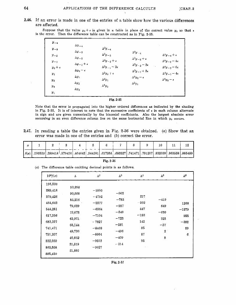
64 APPLICATIONS O F T H E DIFFERENCE CALCULUS [CHAP. 2
X
f(x)
2.46. If an error is made in one of the entries of a table show how the various differences are affected.
Suppose that the value yo + E is given in a table in place of the correct value yo so tha t e is the error. Then the difference table can be constructed as in Fig. 2-35.
Y-4 AY-4
76-3 A2Y -4
AY-3 A3Y -4
AY-2 43y-3 + E
Y-2 4211 - 3 A4y-4 + E
7d- 1 A2y-2 + E A4y-3 - 4~ A3y-z - 3s A Y - 1 - k E
Y O + € A2&1 - 2e A4y-2 + 6~ AYO - E A3y-1 + 3~
Y t A2yo + E A42/ - 1 - 4~ AY 1 A3y0 - E
YZ A2Y 1 ~ 4 y ~ + E
AY2 A3Y 1 Y3 A2Y 2
AY 3 Y4
1 2 3 4 5 6 7 8 9 10 11 12
.195520 .289418 .379426 .464642 .544281 .617356, .683327 .741471 .791207 A32039 363558 .885450
Fig. 2-35
Note t h a t the error is propagated into the higher ordered differences as indicated by the shading i n Fig. 2-35. It is of interest to note t h a t the successive coefficients of e in each column alternate in sign and a r e given numerically by the binomial coefficients. Also the largest absolute error occurring in a n even difference column lies on the same horizontal line in which yo occurs.
2.47. In reading a table the entries given in Fig. 2-36 were obtained. (a) Show that an error was made in one of the entries and ( b ) correct the error.
Fig. 2-36
(a) The difference table omitting decimal points is as follows.
195,520
289,418
379,426
464,642
544,281
617,356
683,327
741,471
791,207
832,039
863,558
885,450
93,898
90,008
85,216
79,639
73,075
65,971
58,144
49,736
40,832
31,519
21,892
-3890
-4792
-5577
-6564
-7104
-7827
-8408
-8904
-9313
-9627
-902
-785
-987
-540
-723
-581
-496
-409
-314
217
-202
447
-183
142
85
87
95
-419
649
-630
325
-57
2
8
1268
-1279
955
-382
69
6,
Fig. 2-37

CHAP. 21 APPLICATIONS O F T H E DIFFERENCE CALCULUS 65
The violent oscillations of sign which occur near the beginning to the column of fourth differences A4 and the practically constant values toward the end of this column indicate an error near the beginning of the table. This is fur ther supported in the column of sixth differences A6. In view of the fact tha t the largest absolute error in an even difference column i s in the same horizontal line as the entry in which the error occurs, i t would seem that the error should occur in the entry corresponding to -1279 which i s largest numerically, It thus appears t h a t the error should be in the entry 0.544281 corresponding to z = 5.
( b ) Denoting the entry which is in possible error, i.e. 0.544281, by yo + E where E is the error, it is clear f rom comparison with the difference table of Problem 2.46 t h a t
A4y--4+e = 217 A4y-3-4e = -202 A4y-z+6e = 447 A4y-1 - 4~ = -183 A4y0+€ = 142
Assuming tha t the correct fourth differences should all be constant, i.e. A4y-4 = A4yds = A42/-2 = A4g-1 = A42/-0, we obtain by subtracting the first two equations, the second and third equation, etc. the equations
5s = 419 or E = 84, 1 0 ~ = 649 o r E = 65, 1 0 ~ = 630 or E = 63, 5e = 325 or E = 65
Because most of these indicate the approximate value B = 65 [the value e = 84 seems out of line] we shall consider this as the most probable value.
Taking into account the decimal point, this leads to E = 0.000065 and so since yo + E = 0.544281, the t rue value should be close to yo = 0.544281 - 0.000065 = 0.544216.
It is of interest to note t h a t the t rue value was actually 0.544218. It appears tha t in copying the table the 1 and the 8 i n this t rue value must have been interchanged.
In Fig. 2-38 the difference table taking into account this error is shown.
106f(x) A A2 A3 A4 A5
195,520
289,418
379,426
464,642
544,218
617,356
683,327
741,471
791,207
832,039
863,558
885,450
~-
93,898
90,008
85,216
79,576
73,138
65,971
58,144
49,736
40,832
31,519
21,892
~~
-3890
-4792
-5640
-6438
-7167
-7827
-8408
-8904
-9313
-9627
-902
-848
-798
-729
-660
-581
-496
-409
-314
~ ~~
54
50
69
69
79
85
87
85
~-
-4
19
0
10
6
2
-2
Fig. 2-38
The changes of sign occurring in the fifth differences could be due to rounding errors as well as the fact tha t the function is not actually a polynomial.

66 APPLICATIONS O F THE DIFFERENCE CALCULUS
X
y
[CHAP. 2
0 0.1 0.2 0.3 0.4 0.5
1.250 1.610 2.173 3.069 4.539 7.029
2.48. Using the following table find the value of y corresponding to x = 0.6.
X 0 0.1
log,, y 0.0969 0.2068
0.2 0.3 0.4 0.5
0.3371 0.4870 0.6570 0.8469
Fig. 2-39
X
0
0.1
0.2
0.3
0.4
0.5
On constructing a difference table from the given data we obtain tha t shown in Fig. 2-40 where we use lO3y in place of y to avoid decimals.
104 log,, Y A A2 A3 A4 A5
969 1099
2068 204 1303 -8
3371 196 3 1499 -5 0
4870 201 3 1700 -2
6570 199 1899
5469
X
0
0.1
0.2
0.3
0.4
0.5
103y A A2 A3 A4 A5
1250
1610
2173
3069
4539
7029
360
563
896
1470
2490
203
333
574
1020
130
241
446
111
205 94
Fig. 2-40
Letting a = 0, h = AX = 0.1 in the Gregory-Newton formula (6) on page 34 we have
or y = 1.250 + 3.60~(~’ + 10.15~(2) I- 21.67~(3) + 46.25~(4) + 78.33~(5) Then the value of y corresponding to x = 0.6 is
y = 1.250 + 3.60(0.6) i- 10.15(0.6)(0.5) + 21.67(0.6)(0.5)(0.4) + 46.25(0.6)(0.5)(0.4)(0.3) + 78.33(0.6)(0.5)(0.4)(0.3)(0.2)
= 11.283
2.49. (a) Work Problem 2.48 by first obtaining logloy in place of y. ( b ) Use the result in (a) to arrive a t a formula for y.
(a) From the table of Fig. 2-39 we obtain the following table.
Fig. 2-42

CHAP. 21 APPLICATIONS O F THE DIFFERENCE CALCULUS 67
Then we find by the Gregory-Newton formula
o r loglo y = 0.0969 + 1.099d1) + 1.02d2) - 0.1333d3) + 0.1250~(4) (1 )
Putting x = 0.6 we then obtain
log10 Y = 0.0969 + 1.099(0.6) + 1.02(0.6)(0.5) - 0.1333(0.6)(0.5)(0.4) + 0.1250(0.6)(0.5)(0.4)(0.3)
= 1.0508
Thus y = 101.0508 = 11.24
(b) The result (1) can be written as
loglo y = 0.0969 + 1.099% + 1 . 0 2 ~ ( ~ - 0.1) - 0 . 1 3 3 3 ~ ( ~ - O.l)(x - 0.2)
+ 0.1250x(~ - O.l)(x - 0.2)(2 - 0.3)
To a high degree of approximation this can be written as
loglo y = 0.0969 + 1.099% + 1 . 0 2 ~ ( 2 - 0.1) = 0.0969 + 1 . 0 2 ~ ~ + 0.9972
0.0969+ 1.0&+0.997x - 10o~ogsg, 101.02x2+0.997x Thus
y = 10 -
(2) - - 1.250. 1ol.02z2+0.997x
The values corresponding to the table of Fig. 2-39 were in fact obtained by using the
(3) formula
x = + x y = 1.250.10
Thus the exact value corresponding to x = 0.6 is 11.40. It is of interest that the value obtained in Problem 2.48 is closer to this true value than that obtained in part (a) using logarithms. This can be accounted for by realizing that in the process of taking logarithms and antilogarithms we introduce small errors each time. Further evidence of this is seen by comparing (2 ) and (3). By recognizing that such errors do occur however we could be led from ( 2 ) t o (3) on replacing 1.02 by 1 and 0.997 by 1. Then (3) could be recognized as the true formula by in fact putting x = 0, 0.1, . . . ,0 .5 and comparing with the corresponding values of the original table.
Supplementary Problems
2.52. Generalize the results of Problem 2.51.
2.54. If yk = k3- 4k2+2k - 3 (d) ( e ) A41/k*
(a) express yk as a factorial polynomial and find (b) Auk , (c)

68 APPLICATIONS O F T H E DIFFERENCE CALCULUS [CHAP. 2
2.55. I f Dk denotes differentiation with respect to k , show that
(a) ( b )
3 Ak = Dk f +Di + &Dk f &D; A: = 0: + Df + &Dt + &Dt + * * a
. . .
(c)
Illustrate Problem 2.55 by finding Af(k5 - 3k4 f 2k3) and check your answer.
A t = Df + $0: + g D i + . . .
2.56.
DIFFERENCE TABLES 2.57. Let f(x) = 5x2+ 3% - 7 where x = 2,5,8,11,14. Set up a difference table for f(x).
2.58. By using only the difference table obtained in Problem 2.57, find the values of x = 17,20,23,26,29,32.
y = f(x) for
2.59. Let f(x) = 2x3 - 8x2 + 6% - 10 where x = 2,4,6,8,10. (a) Set up a difference table for f ( x ) and ( b ) deduce the values of f(x) for x = 12,14,16,18,20 from this difference table.
2.60. (a) Suppose tha t in Problem 2.57 the diRerence table had been set up for values x = 2,5,8,11. Would the resulting table enable us to obtain the values of y = f(x) for x = 14,17,20,23? Explain. (b) Answer par t (a) if the difference table had been set up for values x = 2,5 ,8 and if the values for x = 11,14,17,20 were wanted.
2.61. Suppose t h a t i t is desired t o obtain the values of f(x) = 3x4 - 2x2 + 7 x + 5 for x = 3,7,11,15, 1 9 , . . .,43. What is the minimum number of values which we must obtain directly from f(x) so t h a t from the resulting difference table we can determine the remaining values of f(x)?
2.62. Generalize the results of Problem 2.61 to any polynomial f(x) and any set of equidistant values of x.
2.63. Find the numerical values corresponding to the letters in the following difference table where it i s assumed t h a t there is equal spacing of the independent variable x.
Y AY A2Y A3Y A4Y
F K -1 4
G n
I
Fig. 2-43
2.64. A difference table has one entry in the column Aoy. in the column (a) Ay, (b) y, (c ) A2y.
Determine how many entries there would be
2.65. Generalize the result of Problem 2.64 by determining how many entries there would be in the column Amy if there were a entries in the column Any.
THE GREGORY-NEWTON FORMULA AND APPLICATIONS 2.66. Prove t h a t (a) (kh) (3) = h3k(3), (b) ( k ! ~ ) ( ~ ) = h4kC4).
2.67. Prove tha t Problem 2.6.
( k h ) ( n ) = hnk(n) by using mathematical induction and thus complete the proof in
2.68. Find a formula for the general term uk of a sequence whose first few terms a r e (a) 5,12,25,44, (b) 1,5,14,30,55. What assumptions must you make? Are the results unique? Explain.

CHAP. 21 APPLICATIONS O F T H E DIFFERENCE CALCULUS 69
X
Y
2.6% Given a sequence whose first four terms are 3,7,14,30. general term of the sequence? the assumptions made and whether you feel tha t results obtained a r e unique.
(a) Can you obtain a formula for the State clearly ( b ) Can you find the 10th term of this sequence?
1 2 3 4 5 6
3 3 7 21 51 103
2.70. Suppose tha t in Problem 2.69 the next three terms of the sequence a re given as 61,113,192. What effect if any would this additional information have i n your answer to t h a t problem?
X
sin x
2.71. Find g as a polynomial function in x which fits the data in the folldwing table and state clearly the assumptions which you make in determining this polynomial.
O 0 30 O 60 O 90'
0.00000 0.50000 0.86603 1.00000
X
log,, x
Fig. 2-44
Suppose tha t the values of x corresponding to those of y in the table of Fig. 2-44 a re 1,3,5,7,9,11. Explain how you might obtain y a s a polynomial function in x from the answer to Problem 2.71. Can you generalize the result of your conclusions?
2.72.
5.1 5.2 5.3 5.4 5.5
0.70757 0.71600 0.72428 0.73239 0.74036
X 60 O 61 ' 62' 63 O
sin x 0.86603 0.87462 0.88295 0.89101
2.75. Estimate the error term in Problem 2.74.
64 ' 65'
0.89879 0.90631
2.76. Use the following table to find (a) loglo 5.2374, ( b ) loglo 5.4933.
X 3.12 3.13 3.14 3.15
log10 x 0.49415 j 0.49554 0.49693 0.49831
3.16
0.49969
2.78. Estimate the error terms in (a) Problem 2.76 and (b) Problem 2.77.
2.79. Use the table of Problem 2.74 to find (a) sin68'30', (b) sin45'18' and compare with the exact values.

70 APPLICATIONS O F T H E DIFFERENCE CALCULUS [CHAP. 2
X 0.1
2.81. Determine if there is any difference to your answer for Problem 2.80 if we add t o the table the values of loglo x for x = 3.11 and x = 3.17 given by 0.49276 and 0.50106 respectively.
0.2 0.3 0.4 0.5
2.82. Given the following table find (a) e0.243, ( b ) e0.411.
X 0.00 0.25
erf (x) 0.00000 0.27633
0.50 0.75
0.52049 0.71116
I e5 1 1.10517 1 1.22140 I 1.34986 ~ 1.49182 I 1.64872 I Fig. 2-49
2.83. The gamma function denoted by r (x) is given for various values of x in the following table. Find r(1.1673).
1 z I 1.15 1 1.16 1 1.17 I 1.18 I 1.19 I I r ( x ) 1 0.93304 I 0.92980 I 0.92670 1 0.92373 1 0.92088 I
Fig. 2-50
CENTRAL DIFFERENCE TABLES AND INTERPOLATION FORMULAS 2.85.
2.86.
2.87.
2.88.
2.89.
2.90.
2.91.
2.92.
2.93.
2.94.
(a) Construct a central difference table corresponding to the data of Problem 2.76 by choosing a = 5.2. (a) Use Stirling’s formula to work Problem 2.76(a) and compare with that obtained by use of the Gregory-Newton forward difference formula.
Work (a) Problem 2.77, ( b ) Problem 2.80 by using Stirling’s formula.
Work (a) Problem 2.76, ( b ) Problem 2.77, ( c ) Problem 2.80 by using the Gregory-Newton back- ward difference formula.
Work (a) Problem 2.76, ( b ) Problem 2.77, ( c ) Problem 2.80 by using Bessel’s interpolation formula.
Show how a central difference table can be expressed using the backward difference operator v, v2, v3, . . . . Write the interpolation formulas on page 36 using the “x notation” in place of the “k notation”.
Show how to write Bessel’s interpolation formula using (a) central differences and ( b ) backward differences.
Work Problem 2.83 by using Stirling’s formula with a = 1.17 and compare with that obtained by using the Gregory-Newton forward difference formula.
Use Gauss’ interpolation formula to work (a) Problem 2.76, ( b ) Problem 2.77, ( c ) Problem 2.80, (d ) Problem 2.83.
Derive the second Gauss formula and thus complete Problem 2.18.

CHAP. 21 APPLICATIONS O F T H E DIFFERENCE CALCULUS
X
71
1 2 4 6 7
ZIG-ZAG PATHS AND LOZENGE DIAGRAMS
Y
2.95. Demonstrate the rules f o r obtaining interpolation formulas [see page 371 by obtaining (a) the Gregory-Newton forward difference formula, ( b ) the Gregory-Newton backward difference formula, (c) Gauss' first formula on page 36, (d ) Stirling's formula. Indicate the zig-zag path in the lozenge diagram which corresponds to each formula.
6 16 102 376 576
2.96. By choosing a n appropriate zig-zag path in Fig. 2-6, page 37, obtain an interpolation formula differing from those on page 36.
X 0 (0') n/6 (30')
sin x 0.00000 0.50000
2.97. Explain whether you could find the error term in (a) the Gauss formulas and ( b ) the Stirling formula by knowing the error in the Gregory-Newton forward difference formula.
n/4 (45') n/3 (SO') n/2 (90')
0.70711 0.86603 1.00000
LAGRANGE'S INTERPOLATION FORMULA 2.98. Work (a) Problem 2.71, (b) Problem 2.80 by using Lagrange's interpolation formula.
k 4 5 6 7 8
2.99. ( a ) Find a polynomial in x which fits the da ta in the following table and use the result to find the values of y corresponding to (b) x = 3, (c) x = 5, (d) x = 8.
9
2.102, Show tha t Lagrange's interpolation formula reduces to the Gregory-Newton forward difference formula in the case where the x values a re equally spaced.
TABLES WITH MISSING ENTRIES 2.103. Find the value u2 missing from the following table.
Fig. 2-54
2.104. Find the values zij and ug missing from the following table.
I- I I I I I I I I 302 I I 146 I 192 I Uk I 72 I
Fig. 2-55

72
2.105.
2.106.
2.107.
2.108.
2.109.
2.110.
2.111.
2.112.
k
UIC
APPLICATIONS O F T H E DIFFERENCE CALCULUS [CHAP. 2
0 5 10 15 20
2 92 212 382
( a ) Use the data of Problem 2.101 to find the^ missing entries for sin x corresponding to x = 16O and x = 75O and compare with the exact values. ( b ) Is there any difference between the answers obtained from the method of par t ( a ) and those using the method of Problem 2.101(b)? Explain.
( a ) Find the values of z/ corresponding to x = 3 and x = 5 in the table of Problem 2.99 using Method 1 of Problem 2.28. ( b ) Can you use the method of par t (a) to find the value of y corres- ponding to x = 8?
Find the values ztl, Z L ~ , Z L ~ , Z L ~ from the following table.
If so what is this value?
11 Fig. 2-56
Find the values Z L ~ , Z L ~ , uj, us from the following table.
Year 1930 1940 1950 1960 1970
Fig. 2-57
X
e - X
A sequence is given by U , , , U ~ , U ~ , U ~ , U ~ , U ~ in which all values but u3 are known. fourth differences a r e assumed constant then
Show tha t if
Z L ~ = 0 . 1 ~ 0 - 0 . 5 ~ 1 + U Z + 0 . 5 ~ 4 - 0 . 1 ~ 5
The following table shows the population of the United States for the years 1930 to 1970 at inter- vals of 10 years. Use the table t o find the population for the years (a) 1980 and ( b ) 1962, 1964, 1966 and 1968.
0 0.1 0.2 0.3 0.4
1.00000 0.90484 0.81873 0.74082 0.67032
X
I 122.8 1 131.7 1 151.1 1 179.3 I 205.2 I .~ Population of I United States (millions)
3 5 8 10 11
P(x) I 9 I 35
DIVIDED DIFFERENCES 2.113. (a) Construct a divided difference table corresponding to the data in the following table.
119 205 257

CHAP. 21 APPLICATIONS OF THE DIFFERENCE CAJCULUS 73
X 0
f (2) 40
2.114.
2.115.
2.116.
2.117.
2.118.
2.119.
2.120.
2.121.
2.122.
2.123
2.124.
2.125.
2 3 6 7 8
8 7 136 243 392
( a ) Find a polynomial in 3: which fits the data in the following table and ( b ) obtain values of f(z) corresponding t o x = 5 and x = 10.
Interest rate
Amount of annuity
l&% 2% 23% 3%
23.1237 24.2974 25.5447 26.8704
Fig. 2-61
Work Problem 2.28 using Newton’s divided difference interpolation formula.
Show how to derive Newton’s divided difference formula by assuming an expansion of the form
f(x) = A0 + A,(% - xO) + A,(% - x ~ ) ( x - $1) + * * ‘ + A,($ - x ~ ) ( x - 21). * ( X - x,) and then determining the constants A,, Al, A,, . . . ,A , .
Obtain the Gregory-Newton formula as a special case of Newton’s divided difference formula.
Prove that the value of f(z,, xl, . . ., 2,) remains the same regardless of the arrangement of xo, zl, . . . , x,, i.e. f(z0, xl, . . . , x,) = f(z,, xo, zl, . . . , x , -~) , etc.
Prove that the divided differences of f(x) + g(z) are equal to the sum of the divided differences of f(4 and dx).
Prove that the divided differences of a constant times f(z) is equal to the constant times the divided differences of f(x).
(a) Show that there is a root of z3- x - 1-= 0 between z = 1 and z = 2. ( b ) Find the root in (a). (c ) Determine the remaining roots of the equation.
Solve the equation x3 + 2x2 + 10% - 20 = 0.
Determine the roots of x3 - 3x2 + 2x - 5 = 0.
Solve the equation e - 2 = x. [Hint. Let g = f(x) = e-5 - 2.3
Solve the equation x = 5(1 - e - 2 ) .
INVERSE INTERPOLATION 2.126. Use the data in Problem 2.71 to find the value of x corresponding to g = f(z) = 15 by using
(a) Lagrange’s formula, ( b ) Newton’s divided difference formula and (c) the Gregory-Newton forward difference formula. Compare your results with the exact value.
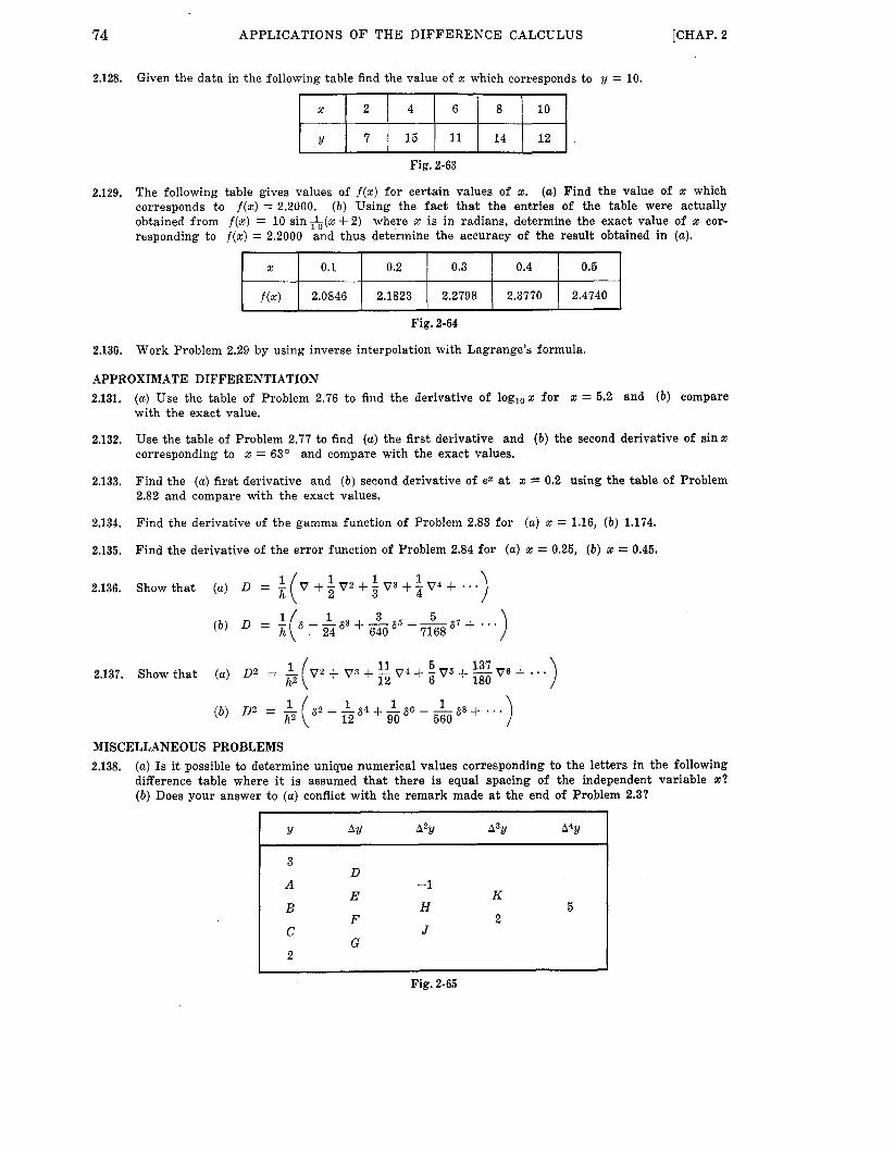
74 APPLICATIONS O F T H E DIFFERENCE CALCULUS [CHAP. 2
f ( x )
2.128. Given the data in the following table find the value of x which corresponds to y = 10.
2.0846 2.1823 2.2798 2.3770 2.4740
1 15 11 14 12
Fig. 2-63
2.129. The following table gives values of f(x) for certain values of x. (a) Find the value of x which corresponds to f ( x ) = 2.2000. (b) Using the fact tha t the entries of the table were actually obtained from f(x) = 10 sin &(x + 2) where x is in radians, determine the exact value of x cor- responding to f ( x ) = 2.2000 and thus determine the accuracy of the result obtained in (a).
I x 1 0.1 I 0.2 I 0.3 I 0.4 I 0.5 I I I I I I I I
APPROXIMATE DIFFERENTIATION 2.131. ( a ) Use the table of Problem 2.76 to find the derivative of logl0z for x = 5.2 and ( b ) compare
with the exact value.
Use the table of Problem 2.77 to find (a) the first derivative and ( b ) the second derivative of sin x corresponding to x = 63O and compare with the exact values.
Find the ( a ) first derivative and ( b ) second derivative of e2 at x = 0.2 using the table of Problem 2.82 and compare with the exact values.
Find the derivative of the gamma function of Problem 2.83 for (a) x = 1.16, (b) 1.174.
Find the derivative of the error function of Problem 2.84 for (a) x = 0.25, (b) x = 0.45.
2.132.
2.133.
2.134.
2.135.
1 1 1 2.136. Show tha t (a) D = V + 2 V2 + 3 V3 + ;i V4 + * * *
11 6 12 6 2.137. Show tha t (a) D2 = Vz + V3 + - V4 + - V j +
MISCELLANEOUS PROBLEMS 2.138. (a) Is i t possible to determine unique numerical values corresponding to the letters in the following
difference table where i t i s assumed t h a t there i s equal spacing of the independent variable X? ( b ) Does your answer to (a) conflict with the remark made at the end of Problem 2.3?
-1
H J
K
2 5
1 Fig. 2-65

75 CHAP. 21 APPLICATIONS O F THE DIFFERENCE CALCULUS
X
&
2.139.
2.140.
2.141.
2.142.
2.143.
44.
2.145.
2.146.
50 52 54 56 58 60
3.6840 3.7325 3.7798 3.8259 3.8709 3.9149
2,
k
Can you formulate a rule which tells the minimum number of entries in a difference table which must be known before all entries can be uniquely determined?
6 8 10 12 14
Ak 1.4258
If a unit amount of money [the principal] is deposited a t 6% interest compounded semi-annually and not withdrawn, the total amount A , accumulated a t the end of k years is given in the following table. Determine the amount accumulated after ( a ) 9 years, ( b ) 16 years.
1.6047 1.8061 2.0328 2.2879
X 0 0.2 0.4 0.6 0.8 1.0
J,(x) 1.0000 0.9900 0.9604 0.9120 0.8463 0.7652 r
Fig. 2-67
Interest rate r
Amount of annuity
Referring to Problem 2.141 after how many years would one expect the money to double?
1 1+ 2 2 8 3
22.0190 23.1237 24.2974 25.5447 26.8704
s 10 20 30 40
f(z) 50.3 42.8 35.6 29.4
A ur
50 60 70 80
22.3 15.5 10.9 6.8
t amount of money deposited a t the end of each year for n years a t an interest rate of r% The following table shows the amount of an annuity
Use the table to determine the amount of compounded annually is called an annuity. accumulated after 20 years a t various interest rates. an annuity after 20 years if the interest rate is 1&%.
A man takes out an annuity [see Problem 2.1441 with an insurance company who agrees to pay back after 20 years an amount equal to 25 times the yearly payment. Determine the interest rate compounded annually which is involved.

76 APPLICATIONS O F T H E DIFFERENCE CALCULUS [CHAP. 2
X 0.1 0.2 0.3
f(x) 0.3423 0.4080 0.5083
2.147. (a) Give a possible explanation for the fact tha t the differences in the table of Problem 2.146 tend to decrease and then increase. ( b ) Does the result produce an error in interpolation? Explain. ( c ) How might more accurate results be obtained?
0.4 0.5 0.6
0.6616 0.9000 1.2790
2.148. The following table gives for various values of x corresponding values of l n r ( x ) where r(x) is the gamma function [see page 701. From the known fact tha t
x r ( x ) r ( l -2) = - sin XT
obtain the values of In r(x) corresponding t o the missing values.
Fig. 2-71
2.149 From the theory of the gamma function we have the result
22=-1r(x) r ( x + 4) = 6132%)
Can this be used in Problem 2.148 to obtain greater accuracy in the values obtained for r(x)? Explain.
2.150. Use Problems 2.148 and 2.149 to find values of l n r ( x ) for x = 0.1,0.2, . . ., 0.9.
2.152. Complete the solution to Problem 2.45 by actually setting the derivative of (1) with respect to t equal to zero.
2.153. Suppose t h a t in Problem 2.45 the times in seconds a r e given by t , = 7.2, t , = 8.1, t3 = 8.4 and t h a t the quantity y at these times has values 15.6, 15.9, 15.7 respectively. Find the time at which y is a maximum and the value of this maximum.
2.154. A t times t , , t,, . . . , t , measured from some fixed time as origin an object is observed to be at posi- tions yl,y2, . . , , y n on a straight line measured from some fixed position as origin. I f ~d i s the position of the object at time t show t h a t
2.155. Show tha t Stirling's interpolation formula can be written in the form
k2 k(k2 - 1) yk = yo + +(Ay-,+Ayo)k + A2Y- - 3(A3Y-2+A3Y-1)- ' 2 ! 3 !
k(k2 - 12)(k2 - 22) - [kz - (n - 1)2] (272 - 1) !
+ ~ 4 y - ~ k2(k2 - ') + + + ( ~ 2 n - l y - ~ + ~ z n - l y - , , + 4 !
+ .. . kz (k z - l2 ) ( k2 -22) . . . [ k z - (n-l),] (2n) ! + A2ny-n
2.156. Referring to Problem 2.44 what estimate of the population would you give for the year 1910? Explain the significance of your result and give possible limitations on the reliability of interpo- lation and extrapolation.

CHAP. 21 APPLICATIONS O F THE DIFFERENCE CALCULUS 77
2.157. Find the sum of the series
[Hint. Find a general term for the sequence 12, l2 + 22, 12 + 22 + 32, . . . .] 12 + 22 + 3* + + k2
2.158.
2.159.
Find the sum of the series (a) 1 + 2 + 3 + * . * + k, (b) l3 + Z3 + 33 i. * .
Find the sum of the first k terms of the series
+ k3.
22 + 52 + 8 2 + 112 + * * *
2.160. (a) Find a formula for the general term of the sequence 2,5,14,31,60,109,194,347, . . . and ( b ) use the result to find the 10th term.
k(1) k(2) k(3) 2.161. Prove t h a t 2k = 1 + - + - + - + . . I l ! 2! 3! for k = 0 ,1 ,2 , . ,
1 k = O 0 k f O '
Show that for k = 0,1,2, . 2.162. Let @k,O = f
2.163. Prove Everett's formula
An advantage of this formula is tha t only even order differences a re present.
2.164. Prove t h a t k(k - 1 ) . * ( k - n + 1)
Yn-2 + ("; 1) F;; 76k = (n - 1) ! [k 1 - (" ') k - n + 2
2.165. Given the following table find the positive value of k such tha t
ykt3 = 3(76k+2-76k) f 18
I I I I I
Fig. 2-73
2.166. Given the following table find the values of k such that
Fig. 2-74
Referring to Problem 2.110(a) estimate the population for the year 1920 and compare with the actual population which was 105.7 million. ( b ) Estimate the population for the years 1910, 1900 and 1890 and compare with the actual populations which were 92.0, 76.0 and 62.9 million respec- tively. ( c ) Estimate the population for the years 1990 and 2000. Discuss the reliability of your predictions.
2.167.

78 APPLICATIONS O F T H E DIFFERENCE CALCULUS [CHAP. 2
X 1 2 3 4 5
f(x) 0.28685 0.36771 0.44824 0.52844 0.60831
6 7 8 9 10
0.68748 0.76705 0.84592 0.92444 1.00263
2.169. Suppose t h a t x = xo is a n approximation to the root of the equation f(x) = 0. Show that under appropriate conditions a better approximation is given by
xo -
and determine these conditions. The method of obtaining roots is called Newton’s method. [Hint. Assume t h a t the exact root is xo + h so t h a t f (xo+ h) = 0. Then use the fact that f ( x o + It) = f ( x o ) + hf’(x,) approximately.]
2.170. Use the method of Problem 2.169 to work (a) Problem 2.37, ( b ) Problem 2.122, (c) Problem 2.123, (d ) Problem 2.124, ( e ) Problem 2.125.
1
THE INTEGRAL OPERATOR We have seen on page 2 that if A and B are operators such that (AB) f = f , i.e. A B = 1,
then B = A-I which is called the inverse operator corresponding to A or briefly the inverse of A .
In order to see the significance of D-' where D is the derivative operator we assume that f(x) and F ( x ) are such that
Then by definition if we apply the operator D to both sides of (1) we obtain F ( x ) = D - ' f ( x ) (1)
(2) D [ F ( x ) ] = D [ D - ' f ( x ) ] = (DD- ' ) f ( x ) = f(x) Thus F ( x ) is that function whose derivative is f(x). know that
But from the integral calculus we
F ( x ) = J - f ( x ) d x + c
D-lf(x) = J f ( x ) d x + c
(3)
where c is the constant o f integration. Thus we have
(4.)
We can interpret D-' or 1 /D as an integral operator or anti-derivative operator.
D-l = J( )dx (5)
The integral in ( 3 ) or (4 ) is called an indefinite integral of f(x) and as we have noted all such indefinite integrals can differ only by an arbitrary constant. The process of finding indefinite integrals is called integration.
GENERAL RULES OF INTEGRATION
integration of functions. we omit the constant of integration which should be added.
I t is assumed that the student is already familiar with the elementary rules for In all cases In the following we list the most important ones.
1-1.
1-2. J L Y f ( X ) dx = J f(x) dx O( = constant
1-3.
J [f(x) + g ( x ) J d x = J f (x ) dx + J g ( x ) d x
s f (x) D g ( x ) dx = f(x) g ( x ) - s g ( x ) D f ( x ) d x
This is often called integrat ion b y parts . d d t ) 1-4. f(x) d x = f [+( t ) ] ,-dt where x = d t )
This is often called integrat ion b y substi tution.
79

80 THE SUM CALCULUS [CHAP. 3
It should be noted that these results could have been written using D-I. Thus, for example, 1-1 and 1-2 become respectively
D - ' [ f ( x ) + g ( x ) ] = D - ' f ( x ) + D - ' ~ ( x ) , Note that these indicate that D-I is a linear operator [see page 21.
D - ' [ d ( x ) ] = a o - ' f ( x )
INTEGRALS OF SPECIAL FUNCTIONS In the following we list integrals of some of the more common functions corresponding
to those on page 5. In all cases we omit the constant of integration which should be added.
11-2. r x m d x m f -1
J m = -1
m # - 1
m = -1
(ax + b)m+' (m + 1)a
In (ux + b) U
11-3. s ( a x + b)"dx =
11-5. s erxdx
bx - In b - -
- sin r x - r 11-7. cos rx d x
b > 0 , b P 1
r i O
r#O
r # O
DEFINITE INTEGRALS Let f(x) be defined in an interval a 5 x 5 b. Divide the interval into n equal parts
of length h = AX = ( b - a) /n . Then the definite integral of f ( x ) between x = a and x = b is defined as
Jb f ( x ) dx = lim i t{f(a) + f ( a + h) + f ( a + 2h) + + f [ a + (n - 1)hl) h - 0
ern-m
if this limit exists. If the graph of y = f ( x ) is the curve C of Fig. 3-1, then this limit represents geometri-
cally the area bounded by the curve c, the x axis and the ordinates a t x = a and x = b. In this figure Xk = U + kh, X k t i = U -k (k -k 1)h and y k = f (Xk) .
I a xk x k + l b
Fig. 3-1
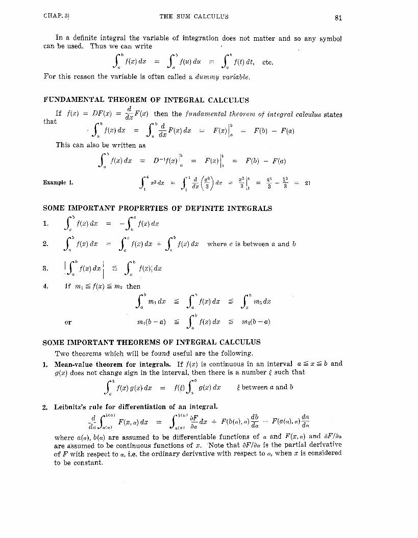
THE SUM CALCULUS 81 CHAP. 31
In a definite integral the variable of integration does not matter and so any symbol can be used, Thus we can write
b
_Jb.’f(x)dx = lb f (u)du = f ( t ) d t , etc.
For this reason the variable is often called a dummg variable.
FUNDAMENTAL THEOREM OF INTEGRAL CALCULUS d dx If f ( x ) = DF(x) = -F(x ) then the f u n d a m e n t a l theoyem o f integral calculus states
that ’ d b
f ( x ) d x = ,,F(z) dx = F(x) Ia = F(b) - F(a)
This can also be written as
= F(x$ = F ( b ) - F ( u )
Example 1.
SOME IMPORTANT PROPERTIES OF DEFINITE INTEGRALS
2. lb f(x) dx = 1‘ f(x) dx + 1’ f (x) dx where c is between a and b
or
SOME IMPORTANT THEOREMS OF INTEGRAL CALCULUS Two theorems which will be found useful are the following.
1, Mean-value theorem for integrals. If f (x) is continuous in an interval a 5 x d b and g(x) does not change sign in the interval, then there is a number t such that
_Jb.’ f ( x ) g(x) d x = f ( t ) J b g(x) dx t between a and b
2. Leibnitz’s rule for differentiation of an integral.
where U ( N ) , b(a) are assumed to be differentiable functions of a and F(x ,a) and dFlaa: are assumed to be continuous functions of x. Note that aF‘laN is the partial derivative of F with respect to (Y, i.e. the ordinary derivative with respect to N , when x is considered to be constant.

82 THE SUM CALCULUS [CHAP. 3
THE SUM OPERATOR Because of the analogy of D and A [or more precisely.A/Ax = A/h], i t is natural to seek
the significance of the operator A-' which we conjecture would have properties analogous to those of D-I.
To discover the analogy we suppose that F ( x ) and f(x) are such that
(6) A
- F ( x ) = f (x) or AF(x) = hf(x) Ax Then by definition A-' is that operator such that
F ( x ) = A-'[hf(x)] (7)
Now we can show [see Problem 3.101 that A-I is a linear operator and also that if two functions have the same difference, they can differ a t most by an arbitrary function C ( x ) such that C(x + h) = C(x) , i.e. an arbitrary periodic function with period h. Since this is analogous to the arbitrary constant of integral calculus we often refer to it as an arbitrary periodic constant or briefly periodic constant.
From (7) we are led by analogy with formulas ( 3 ) and (4) of the integral calculus to define
o r a-'[f(x)l where CI(X) is also a periodic constant.
which displays the remarkable analogy
D-'f (x)
= c f (x) + Cdx) (9)
It is of interest that (9) can be written as
= c f(x)Ax + C ( x ) (10)
with
= J-f(x)dx + c (14
We shall call B the sum operator and B f(x) [or Z f(x) Ax = h B f(x)] the indefinite sum of f(x). Note that because of (9) and (10) we can consider A-' and B or A l A x and Z ( ) A x as inverse operators, i.e. A B = 1 or B = A-'. See Problem 3.11. The process of finding sums is called summation.
GENERAL RULES OF SUMMATION
In all cases we omit the periodic constant of summation which should be added. The following formulas bear close resemblance to the rules of integration on page 79.
111-1. c [f(4 +g(x)] = c f ( x ) + c g(x)
111-3. c f ( x ) u ( x ) = f(x) Q(4 - c g(x + h) A f ( 4
111-2. c af(X) = a c f ( x ) (Y = constant
This is often called sumnzation by parts. Note that these formulas could have been written using A-1 instead of 8. The first
two represent the statement that B or A-' is a linear operator.

CHAP. 31 THE SUM CALCULUS 83
SUMMATIONS OF SPECIAL FUNCTIONS In the following we list sums of some of the more common functions. The results are
analogous to those on page 80. In all cases we omit the periodic constant which should be added.
f f X - - - h IV-1. c ff
X ( m + l ) - - (m + 1)h m # - 1
For the case where m = -1 or is not an integer we use the gamma function [see page 861.
IV-4. c bx IV-5. 2 erx
cos Y ( X - 3h) - - - 2 sin drh IV-6. c sinrx
sin r ( x - Ah) 2 sinfrrh
- - IV-7. 2 cosrx
These results can also be written with in place of H. The analogy of the above For example, with corresponding integrals is clear if we multiply the sums by h = Ax.
IV-2 becomes
which corresponds to
with h = Ax, xcm) and H corresponding to dx, xm and $ respectively.
This relationship between the sum calculus and integral calculus is expressed in the following important theorem.
r 1 n
Theorem 3-1.
DEFINITE SUMS AND THE FUNDAMENTAL THEOREM OF The definite sum of f(x) from x = a t o x = a + (n - 1)h in steps
a + ( n - l l h
a C f(x) = f ( a ) + f (a + h) + f ( a + 2h) + * * - + f[a +
SUM CALCULUS of h is denoted by
The following theorem analogous to the fundamental theorem of integral calculus on page 81 is of great importance and is called the fundamental theorem of the sum calculus.
Theorem 3-2 [fundamental theorem of sum calculus]. a + ( n - l ) h

84 THE SUM CALCULUS [CHAP. 3 C
where it is emphasized once again that the sum on the left is taken from x = a to x = a + (n -- 1)h in steps of h. It should also be noted that the right side of (15) means that the indefinite sum is to be found as a function of x and we are then to substitute the upper limit a+nh and lower limit a and subtract the results. In such case the added arbitrary periodic constant is subtracted out as in the case of definite integrals.
Example 2. If a = 1, h = 2, n = 3, then from (15) and IV-2 we have
This checks since the left side is (1)(-1) + (3)(1) + (5)(3) = 17.
It is of interest to note that if we multiply both sides of (15) by h and then let h + 0 and n + so that nh = b - a, we obtain the fundamental theorem of integral calculus.
DIFFERENTIATION AND INTEGRATION OF SUMS The following theorems are sometimes useful.
Theorem 3-3. If A-'F(X) = BF(x) = G(x) then 4--1(g) = 2 - dF = - dG dx dx
Theorem 3-4. If a-'F(x,a) = BF(x ,a ) = G(x,~t ) then
Theorem 3-4 is analogous to Leibnitz's rule for differentiating an integral [see page 811.
Similar results hold for integrals. For example we have
Theorem 3-5.
THEOREMS ON SUMMATION USING THE SUBSCRIPT NOTATION
can be expressed in terms of the subscript notation yk = f ( a + kh). page 82 becomes using Zk = g ( a + kh)
As in the case of the difference calculus all of the above results for the sum calculus For example 111-3 on
c zjicaZk = YkZk - c Zk+lAyk (16 )
The periodic constant of summation in this case becomes an arbitrary constant.
Similarly formulas IV-1 through IV-7 can be written with x replaced by k and h = 1. For example, IV-2 becomes k ( m + l )
2 k ( m ) = - m i - 1 (17) m + l The fundamental theorem of sum calculus can in subscript notation be written, using the particular value a = 1, as
n+l
$ y k = A-%k I I k = l
It is seen that the subscript notation has some obvious advantages since h does not a p p e a F .

CHAP. 31 THE SUM CALCULUS 85
ABEL'S TRANSFORMATION The following result, called Abel's transformation, is sometimes useful.
n k
Ukvk Untl v k - 5 [ A u k p z k = l k = l k = l (19)
OPERATOR METHODS FOR SUMMATION
One useful result valid for p # 1 is given by Various operator methods are available which can be used to obtain summations quickly.
P(k) ---pkP(k) = pk- 1 1
E - 1 ,BE - 1 1 A BkP(k) = A-'[pkP(k)] = -pkP(k) =
where c is an arbitrary constant. The series terminates if P(k) is a polynomial.
SUMMATION OF SERIES The above results are very useful in obtaining sums of various series [see Problems
3.20-3.281. Further applications involving the important topic of summation of series are given in Chapter 4.
THE GAMMA FUNCTION
use of the gamma function. This function is defined by In order to generalize the factorial x ( ~ ) to the case where m is not an integer we make
r(p) = t P - l e - t d t = M - t o l lim xM t p - ' e c t d t p > 0 (21)
and we can show [see Problem 3.321 that
The recursion formula (22) can be used to define r(p) for p 5 0 [see Problem 3.34(c)]. r ( p + 1) = W(P) (22)
Some important properties of the gamma function are as follows.
1. If p is a positive integer, r (p + 1) = p !
2.
3.
4.
where
If m is an
Since (23) has
r(+) = fi
O < r < l x r (r )r ( l - r ) = - sin r?:
r'(1) = Jffi e- t ln t d t = -7 = -0.5772156649.. . 0
y is called Euler's constant.
integer we can write [see Problem 3.351
hmr (i + 1) X(m) =
meaning for all values of m we shall take it as a definition of x ( ~ ) for all m.

86 THE SUM CALCULUS [CHAP. 3
and
thus generalizing the results (25) , page 6, and IV-2, page 83.
If m = -1, we obtain [see Problem 3.391
The function on the right of (26) is sometimes called the digamma function and is denoted
The results (23) through (26) can also be written in the “k notation” with k replacing by qx).
x and h = 1.
BERNOULLI NUMBERS AND POLYNOMIALS Various sequences of functions fo(x),f~(x), f z ( x ) , . . . have the property that
D f n ( x ) = f n - l ( x ) (27) where in (27), as well as what follows, we shall assume that n = 1,2,3, . , . . sider the function f n ( x ) to be a polynomial of degree n then we can show that
If we con-
coxn c1xn-1
n ! ( n - l ) ! fn(x) = - +-+ . . . + C n - I X + Cn
where CO, CI, . . . , en are constants independent of n [see Problem 3.401.
given. Different conditions will result in different sequences of polynomials. To specify the polynomials, i.e. to determine CO, CI, . . ., Cn, further conditions need to be
Let p,(x) be a sequence of polynomials satisfying (27), i.e.
OP,(x) = P,&)
@ n ( x ) = (n - 1) ! and the added condition p - 1
where we take h = 1 and define O ! = 1, Conditions (29) and (30) enable us to specify completely the polynomial p,(x). We find in fact that the first few polynomials are
See Problem 3.41.
It should be noted that once p,(x) is found, we can use (29) t o find P,-,(x), Pn-2(x), . . . , by successive differentiations. This is particularly useful since i t is possible to obtain P,,(x) in terms of Stirling numbers of the second kind by the formula
Po@) = 1, /3,(x) = x - 4, &(x) = - &x + A, &(x) = Qx3 - *x2 + &x (31)
See Problem 3.44.
We define the Bernoulli polynomials as
B,(4 = n!P,(x) (33)
so that from (32)

CHAP. 31 THE SUM CALCULUS 87
The first few Bernoulli polynomials are given by
Bo(x) = 1, Bi(x) = x - 6 , Bz(x) = X' - x + 9, B ~ ( x ) = x3 - $ x 2 + 4% (35) We define the Bernoulli numbers, denoted by Bn, as the values of the Bernoulli poly-
nomials with x = 0, i.e. Bn = Bn(0) (36)
The first few Bernoulli numbers are given by
Bo = 1, B1 = -4, Bz = 9, B3 = 0 , Bq = -&j (37) For tables of Bernoulli numbers and polynomials see Appendixes C and D, pages 234
and 235.
IMPORTANT PROPERTIES OF BERNOULLI NUMBERS AND POLYNOMIALS
numbers and polynomials. In the following we list some of the important and interesting propyties of Bernoulli
1. B,(x) = xn + (Y)xn-lBl + ( ~ ) X , - ~ B Z + * + (:>Bn
This can be expressed formally by B,(x) = (x + B)" where after expanding, using the binomial formula, Bk is replaced by Bk. It is a recurrence formula which can be used to obtain the Bernoulli polynomials.
2.
3. B;(x) = nB,-i(x)
B,(x + 1) - B,(x) = nxn-l
4. B, = B,(O) = Bn( l ) , B2n-l = 0 n = 2 , 3 , 4 , . . .
5 .
This can be expressed formally as (1 + B)" - Bn = 0 where after expanding, using the binomial fomda, Bk is replaced by Bk. This recurrence formula can be used to obtain the Bernoulli numbers.
7.
8.
9.
10.
This is often called the generating function for the Bernoulli polynomials and can be used to define them [see Problems 3.51 and 3.531.
This is called the generating function for the Bernoulli numbers and can be used to obtain these numbers [see Problem 3.521.
X X B~x' + - + - B4x4 B6X6 + . . . 4 ! 6 ! -cothZ = 1 + 2
(n + B)'+' - Brtl 1' + 2' + 3' + * * * + (n-1)' = r + l
where r = 1,2 ,3 , . . , and where the right side is to be expanded and then Bk replaced by Bk.

88 THE SUM CALCULUS [CHAP. 3
11. ( -l)n-1B2n(2x)2n n = 1,2,3, . . . - + - + - + . . . 1 1 1 =
12n 22" 32n 2 - (2n) !
12. If n = 1,2,3, ., . . , then ffi sin2kii-x Bz,-l(x) = 2(-1)"(2n - I ) !
k = l (2kT)'"-'
EULER NUMBERS AND POLYNOMIALS The Euler polynomials E,(x) are defined by equation (27), i.e.
DEn(x) = E,-I(x) together with the added condition
(39) X n X n MEn(X) = - or +[E,(x+ 1) + E,(x)] = a n !
where M is the averaging operator of page 10 and h = 1.
The first few Euler polynomials are given by
Eo(x) = 1, El(%) = x - 4, E ~ ( x ) = ax2 - +x, E ~ ( x ) = +x3 - + +g (40) The Euler numbers are defined as
En = 2"n! En(+) (41)
Eo = 1, El = 0, Ez = -1, EB = 0, E4 = 5, Eg = 0 (42)
and the first few Euler numbers are given by
For tables of Euler numbers and polynomials see Appendixes E and F, pages 236 and 237.
IMPORTANT PROPERTIES OF EULER NUMBERS AND POLYNOMIALS
bers and polynomials. In the following we list some of the important and interesting properties of Euler num-
1.
2.
3.
4.
5.
6.
7.
where
'oxn + . . . + + en E n ( ~ ) = - n! + - ( n - l ) !
The first few values of e k are 1 eo = 1, el = --&, e2 = 0, e3 = &, e4 = 0, e5 = -m
E;(x) = En-l(x)
E,(x) = (-l)nE,(l- x )
E,(O) + E,(1) = 0 for n = 1,2,3, . . .
for n = 1,2,3, . . .
fo r n = 1,2,3, . . .
2(-1)" E,(O) + En(-l) = - n !
Epn = 2*"(2n)! Ezn(&) = 0
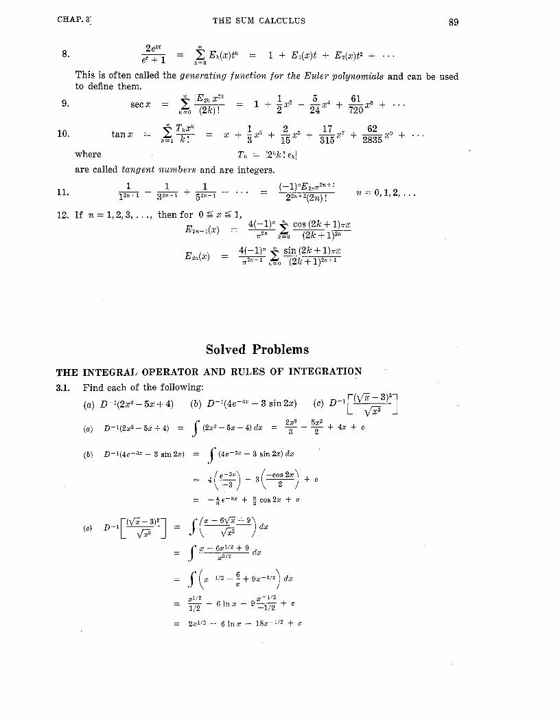
CHAP. 31 THE SUM CALCULUS 89
8.
9.
10.
11.
This is often called the generating funct ion f o r the Euler polynomials and can be used to define them.
secx = 2 i E 2 k l X 2 k = 1 + - - 2 1 + -x4 5 + -x6 61 + . . . k=O ( 2 k ) ! 2 24 720
2 - - TkXk 1 2 17 x i- 62 x 9 + . . . 2835
- x + - x 3 + -x5 + - ' 3 15 315 t anx =
k = l k ! where Tk = / z k k ! ek l
are called tangent numbers and are integers.
12. If n = 1 , 2 , 3 , . . . , thenfor Odxdl,
Solved Problems THE INTEGRAL OPERATOR AND RULES OF INTEGRATION 3.1. Find each of the following:
(a ) D-'(2x2 - 5% + 4) (b ) D-1(4e-3" - 3 sin 2x) (c ) Ddl[
+ 4 x + c (a) 0-'(222- 5 2 + 4) = (222-5% + 4) dx = - - - 2x3 5 % ~ S 3 2
( b ) D-1(4e-3" - 3 sin 2x) = r (4e-3" - 3 sin 2x) dz J
$1/2 x-1/2
112 - - 61nx + 9- + c

90 THE SUM CALCULUS [CHAP. 3
3.3. Find (a) s x cos4x dx, ( b ) 1 In x dx.
(a) We use integration by par ts here. Let f(x) = x, Dg(x) = cos4x
so tha t sin 42 4 D f ( x ) = 1, g(x) = -
where in finding g(x) we omit the arbi t rary constant.
Then using the formula for integration by parts,
+ C x s in4x C O S ~ X +- 4 16
+ ( sin44x) - J sin442 cis = x cos4x dx = x- S ( b ) Let f ( x ) = lnx , D g ( x ) = 1 so tha t
1 D f ( 4 = ;, d x ) =
Then using integration by par ts we have
l n x d x = x l n x - = x l n x - x s 3.4. Find (a) sx2e3 ' .dx , ( b ) x4 sin2x dx.
(a) In this case we must apply integration by par ts twice. We obtain s x2e3x dx = (x2) (7) - S ( 2 x ) (7) d x
= (~2 ) (? ) - [ (2%) ($) - s ( 2 ) ( $ ) d x ]
= (%2)($) - ( 2 4 3 + (2)($)
a p a r t from the additive constant of integration.
I n this result we make the following observations.
The Erst factors in each of the last two terms, i.e. 2% and 2, a r e obtained by taking suc- cessive der iva t ives of x2 [the first factor of the first term].
The second factors in each of the las t two terms, i.e. e35/9 and e3x/27, are obtained by taking successive in tegrals of e3"/3 [the second factor of the first term].
(iii) The signs of the terms alternate +, -, +. The above observations a re quite general and can be used to write down results easily in cases where many integrations by par ts might have to be performed. A proof of this method which we shall refer to as generalized in tegrat ion by par t s is easily formulated [see Problem 3.1431.
(i)
(ii)
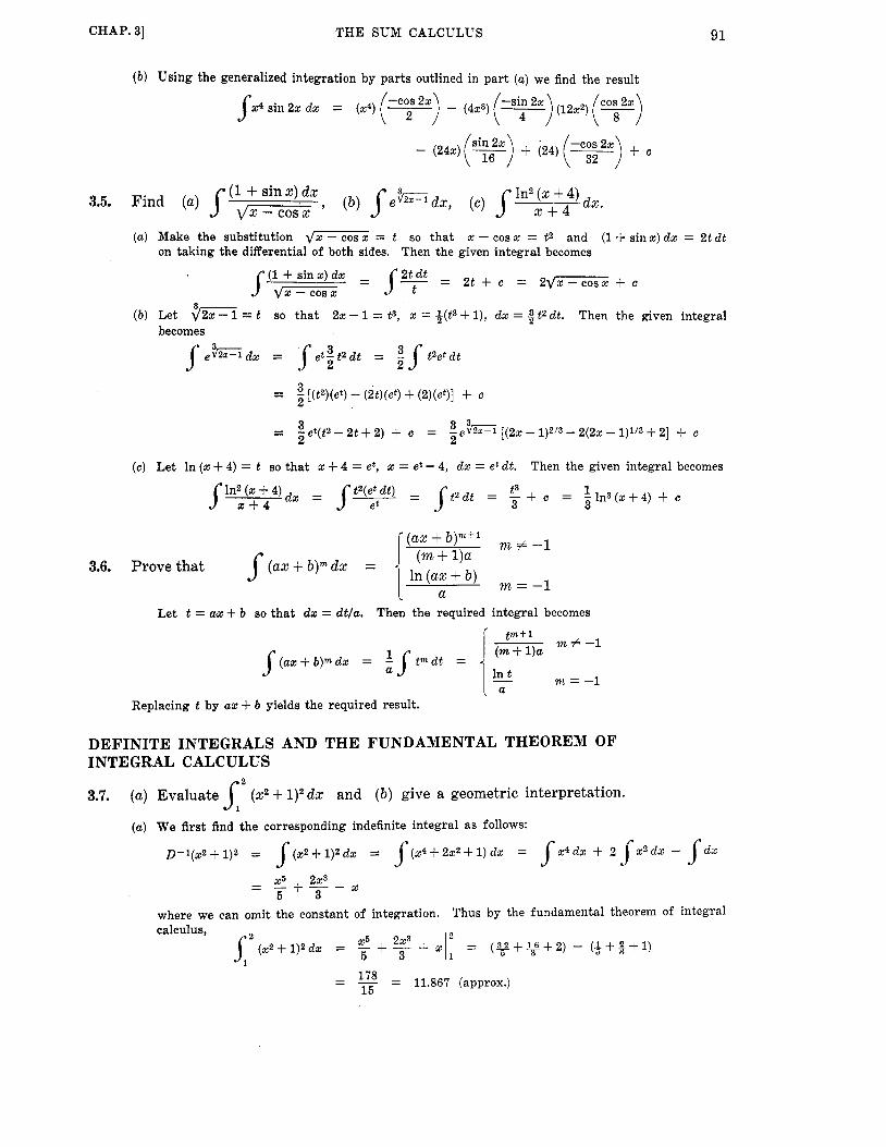
CHAP. 31 THE SUM CALCULUS 91
( b ) Using the generalized integration by parts outlined in part (a) we find the result
3c4 sin22 dx = (x4) S - ( 2 4 z ) ( y ) + (24) (9) + c
(1 + sin x) dx f ( b ) Je\"dx, (4 J In2 (x + 4 + 4) dx. v x - cos x 3.5. Find (a) J
(a) Make the substitution q x - cosx = t so that x - cosx = t z and (1 + sinx) dx = 2t dt on taking the differential of both sides. Then the given integral becomes
S ( l + s i n x ) d x = sy = 2 t + c = 2q-f c v x - cosx
3 ( b ) Let d- = t so that 22 - 1 = t3, x = 8(t3 + l), dz = Qtzdt. Then the given integral
becomes
$ e k = i & = S e t i t z d t = zs 2 t2etdt
=
= i e t ( t2 -2 t+2) + c = 3 e ~ [ ( ~ s - l ) 2 / 3 - 2 ( 2 x - l ) 1 / 3 + 2 1 2 + c
[(tZ)(et) - (it)(et) + (2)(et)] + c
3
(c) Let In (x + 4) = t so that x + 4 = et, x = et - 4, dx = et dt. Then the given integral becomes
Let t = ax + b so that dx = dtla. Then the required integral becomes
Replacing t by ax + b yields the required result.
DEFINITE INTEGRALS AND THE FUNDAMENTAL THEOREM OF INTEGRAL CALCULUS
2
3.7. (a) Evaluate (x2 + 1)2 dx and ( b ) give a geometric interpretation.
(a) We first find the corresponding indefinite integral as follows:
D-1(x2+1)2 = J (x2+l )zdx = J (x4+2x2+l)dx = s z 4 d x + 2Jx2dx + J d s
where we can omit the constant of integration. calculus,
Thus by the fundamental theorem of integral
11 3 %5 2x3 (&+1)2dx = - + - + x = (y+u+2) - ( & + Q + l ) 5 3
15 - _ - 178 = 11.867 (approx.)

92 THE SUM CALCULUS [CHAP. 3
( b ) The value 178/16 = 11.867 (approx.) represents the area [shaded in Fig. 3-21 bounded by the curve ld = (x2+ the x axis and the ordinates a t x = 1 and x = 2.
X
Fig. 3-2
3.8. Find (a) SnI2 sin 6x dx, ( b ) J2 ~ e - ~ ~ d x , (C) iz x2 -% + 2 . 0
(c) Method 1. d x dx s x2 - 22 + 2
Let x - 1 = tan t. Then d x = see2 t d t and so
= S d t = t + c = tan-'(x-1) + c,
Thus
Method 2.
and when x = 2, tan t = 1, t = id4 As in Method 1 we let x - 1 = tan t but we note that when x = 0, tan t = -1, t = -d4
Then
77 d x dx - JVl4 sec2t d t = JTi4 at = - 2 t = --a/4 tan2 t + 1
t = -7r/4
Note that all of these can be interpreted geometrically as an area.
THE SUM OPERATOR AND RULES OF SUMMATION
3.9. A A
Prove that if ~ F I ( x ) = f(x) and z F z ( x ) = f(x), then Fl(x) - Fz(x) = c(x) where C(x + h) = C ( x ) .

CHAP. 31 T H E SUM CALCULUS
By subtraction we have
93
A Ax or -[Fl(x) - F 2 ( x ) ] = 0 i.e. AIFl(x) -F,(x)] = 0
If we write Fl(z) - F 2 ( 2 ) = C ( x ) then AC(x) = 0 or C ( x + h) - c(z) = 0, i.e. C(z + h) = C ( x )
We refer to C ( x ) as a periodic constant with period h. We have proved tha t if two functions have the same difference, then they can differ by at most a n arbi t rary periodic constant, The result i s analogous to the theorem of integral calculus which states tha t two functions which have the same derivative can differ at most by a n arbi t rary constant.
3.10. Prove that A-' is a linear operator, i.e. (a) A-'[f(x) 4- g(x ) ] = A-'f(x) + A-'g(x) and ( b ) a-'[.f(x)] = .A-lf(x) where f(x) and g(x) are any functions and (Y is any constant. (a) By definition if AF(x) = f(x) and AG@) = g(x) then
F ( x ) = A-lf(x), G(x) = A-'g(z) (1)
Also by adding AF(z) = f(z) and 'AG(x) = g(x) we have
A[F(z) + G(z)l = f(x) + g ( 4 so that by definition
Using (1) in (2 ) we find as required
F ( x ) + G ( 4 = A-'[f(x) + g(x)I
A-l[f(x) + g(x)] = A-lf(x) + A-lg(x)
( b ) F o r any constant (Y we have
Thus from the first equation in (1)
A[aF(%)] = aAF(x) = (Y~(x)
A-'[af(%)] = &(x) = aA- l [ f (~ ) ]
3.11. If we define P(x) = a- l [hf (x) ] = Bf(x)h + C ( x ) as in (S), Page 82, prove that (a) A X = 1 or B = Ad', ( b ) A-'[f(x)] = B f(x) + Cl(x) where CI(X) is an arbitrary periodic con-
stant, and (c) (&)-I f(x) = 2 f(x) A x -I- c(X). By operating with A on
F(x ) = A - l [ h f ( z ) ] = x f ( x ) h + c(o)
AF(x) = h f ( z ) = A x f ( x ) h -I- Ac(x)
Now by Problem 3.9, AC(x) = 0 so that ( 2 ) becomes
we obtain
since A is a linear operator.
h f b ) = A x f ( d h
But since f(x) is arbi t rary and h # 0 i t follows from (8) t h a t
A X = 1 or 2 = ~ - 1
It follows from this and Problem 3.10 tha t B is a linear operator.
Dividing equation (1) by h using the fact tha t B and A-1 are linear operators, we have
where C(x) and thus Cl(x) = C(x) /h are periodic constants.

94 THE SUM CALCULUS
(c) This follows a t once from (1) on noting that
[CHAP. 3
and replacing h by Ax.
3.12. Prove that (a) B [f(x) +g(x)] = Bf(x) + z g ( X ) , ( b ) B d ( X ) = a z f (x ) . These follow a t once from the fact that = A--l and Problem 3.10.
3.13. Prove the formula fo r summation by parts, i.e.
x'"+l' - cos r ( x - gh) m z -1, ( b ) B sinrx = (m+l)F, ' 2 sin &rh 3.14. Prove (a) B d m ) =
(a) We have from V-2, page 7, or (24), page 86, on replacing rn by m + 1
Ax(m+1) = (m 4- l ) x ( m ) h
Then if m # -1,
i.e.
or
apart from an additive periodic constant.
( b ) From V-7, page 7,
AIcosrm] = -2
Replacing x by x - i h , we have rh 2 A[cos r ( x - *h)] = -2 sin- sin r x
rh 2 Thus on dividing by -2 sin - , we have
sin rx -2 sin 3rh 1 - - cos r ( x - i h )

CHAP. 31
so that
THE SUM CALCULUS 95
cos r(x - +h) 2 sin &rh
A - 1 s i n r s = - or
cos r (z - +h) 2 s inah
2 s inrx = - apart from an additive periodic constant. L
3.15. Use Problem 3.14(b) to obtain s inrx dx. S From Problem 3.14(b) we have on multiplying by h
h cos T ( Z - &h) 2 h s i n r x = - 2 sin &rh
Letting h + 0 this yields h cos r(5 - &h)
s i n m dx = lim - S h-rO 2 sin&&
-cos r(x - ")I[ i r h 3 -cos r(x - @)I[ ]
= lim [ h+O sin i r h
= [ lim lim - h+O r h - 0 sin +rh
The arbitrary periodic constant C(x) becomes an arbitrary constant c which should be added to the indefinite integral. The result illustrates Theorem 3-1, page 83.
3.16. (a) Find A-'(xax) = B xu2, a # 1, and (b ) check your answer.
(a) We have from Problem 3.13
A - l [ f ( ~ ) A d z ) ] = f (z) &) - A - ' [ d s -I- h) A f ( s ) ]
Let f(z) = x and A&) = ax. Then A f ( z ) = A x = h and
ax a h - 1 g(2) = A- laZ = -
Thus
hax+h - x a x - ah - 1 ( a h - 1 ) 2
( b ) Check:
(ah - 1)(x + h ) a Z + h - haz+2h - ( a h - l ) ( x a s ) + has+h (ah - 1 ) 2
x a x

96 THE SUM CALCULUS [CHAP. 3
DEFINITE SUMS AND THE FUNDAMENTAL THEOREM OF SUM CALCULUS 3.17.
3.18.
Prove Theorem 3-2, the fundamental theorem of sum calculus, i.e. a + ( n - l l h
a c f ( x ) = a-Y(a)la+nh
If we assume that F(z) and f(x) are related by
(1 )
we have F(z + h) - F ( x ) = hf (z ) (8)
- - AF(x) - f(z) or AF(X) = hf(x) Ax
Then by putting x = a, a + h, . . . , a + (n - 1)h successively in (2) we obtain the equations F(a+ h) - F ( a ) = hf(a) F(a + 2h) - F(a + h) = h f (a + h)
F(a + nh) - F [ a + (n - l)h] ...........................................
= h f [a + (n - l)h]
Thus by addition we have
F(a + nh) - F(a) = h{ f (a ) + f ( a + h) + * - * + f [ a + (.n - l)h]}
or
where the sum is taken from x = a t o a + (n- 1)h in steps of h.
But from the second equation in (1) it follows that
and the required result is proved on
Evaluate each of the following verify directly
(a) 2 8 ~ ' ~ ) if h = 3 7
1
using this in (8).
using the fundamental theorem of sum calculus and
277
0 (c) c cos 5x if h = d 2
6 19
2 3 (b) 2 [ 3 ~ ( ~ ) - 8 x ( ~ ) + 101 if h = 2
(a) Since 2 8 d 3 ) = 8 2 x ( 3 ) = 8 4 . 3 = 3
(d) c if h = 4
~ ( 4 ) 20(4) we have by the fundamental theorem of sum
calculus using a = 1 and It = 3,

CHAP. 31 THE SUM CALCULUS 97
Check: 5 2 [3d2) - 8d1) + 101 = [3(2)(0) - 8(2) + 101 + [3(4)(2) - 8(4) + 101 + [3(6)(4) - 8(6) + 101 = 30 2
(c) By IV-7, page 83, with T = 5, h = a/2 we have
Thus
sin 512 - ( ~ / 4 ) ] 2 sin (5d4) A-1 C O S ~ Z =
2Tl 2 cos5s = 0
sin 5[2 - (d4) ] 5 ~ 1 2
2 sin (5d4) o
- sin (45d4) - sin (-5d4) = - 2 sin (5r/4) 2 sin (5d4)
Check: 2a
2 cos5a: = COSO + C O S ( ~ ~ T / ~ ) + C O S ( ~ T ) + ~ 0 ~ ( 1 5 a / 2 ) + cos( l0r) = 1 0
Check: 25 - - 19 1 1 1 1 Xs(-3) = ___ + ~ - 4347 3 3 . 7 0 1 1 7 - 1 1 . 1 5 + 1 1 * 1 5 * 1 9 + 1 5 - 1 9 . 2 3
DIFFERENTIATION AND INTEGRATION OF SUMS 3.19. Find A-l[xerz] by using Theorem 3-4, page 84.
We have from IV-5, page 83, erz ~ - l [ e r z ] = -
erh - 1
Then by differentiating both sides with respect t o r [which corresponds to a in Theorem 3-41 we find
(erh - l)(zerz) - (e")(herh) (erh - 1)2 A-I[zerz] = or
- ( x - h)er(z+h) - se'z - (erh - 1)2
This can be checked by referring to an alternative method of obtaining the result given in Problem 3.16(a). From that problem we find on putting a = er
her(%+ h ) - ($ - h)er(z+h) - Zerz A - ~ [ x ~ ? Z ] = - - - - erh - 1 (erh - 1)2 (erh - 1 ) 2
SUMMATION OF SERIES 3.20. Sum the series 1 . 3 - 5 + 3.507 + 507.9 + to n terms.
Since the nth term of the series is (2% - 1)(2n + 1)(2n + 3), the series can be written as 2n.e 3
5 2 x ( 3 ) where h = 2

98 THE SUM CALCULUS [CHAP. 3
Then by the fundamental theorem of sum calculus,
- (2n + 5)(2n + 3)(2n + 1 ) ( 2 ~ - 1) - (5)(3)(1)(-1) 8 8
-
- (2n + 5)(2n + 3)(2n + I)(2n - 1) + 15 8 -
3.21. Sum the series (a) l2 + 22 + 32 + 42 + and ( b ) 22 + 5' + 82 + 112 + . to n terms. Since we wish to find X 2 2 we need to express x 2 as a factorial polynomial. This is found from
3 2 = X ( 2 ) + hxcl)
As a possible check we can t r y a particular value of n, say n = 3. Then we obtain
(2)(3)(7) = 14 1 2 + 22 + 32 = ~ 6 which is correct.
( b ) The nth term is (3% - 1)2. Thus using h = 3 the series can be represented by
(3% + 2)(3n - 1)(3n - 4) (3% + 2)(3n - l)] - p2)(-1)(-4) I (2)(-1)] = c 9 2 9 2 + (3% + 2)(3n - l)(6n + 1) 4- 2 - n(6d + 3% - 1) - - -
18 2
Check: Let n = 3. Then (3)(6 ~3~ + 3 . 3 - 1) = 93
2 22 + 6 2 + 82 = which is correct.
to n terms. 1 +-----+-----+ 1 1 . . . 3.22. Sum the series ~ 1 0 3 . 5 3 . 5 . 7 5 .709
1 The n th term of the series is (2n - 1)(2n + l)(2n + 3) .
Now since 1 ( % - h ) ( - 3 ) = -
x(z + h)(x + 2h)
i t follows tha t if we let h = 2, the required sum of the series is

CHAP. 31 THE SUM CALCULUS 99
= L- 1 12 4(2n + l)(2n + 3)
Check: Putting n = 2 we find - 1 + - 1 - - 1 - - 1 - which is correct. 1 . 3 . 5 3 . 5 0 7 - 12 4(5)(7) - 105
3.23. Sum the series 1.3.5 1 + 3.5.7 1 + 5.7.9 1 + - * . In this case we are to sum the series of Problem 3.22 to infinitely many terms. The required
sum using the result of Problem 3.22 is
lim [L- ]= . 1 n e w 12 4(2n + 1)(2n + 3)
3.24. Sum the series + + cos 0 + cos 20 + . + cos no. Using h = e the series is given by
1 sin ( n + + ) e -- s i n i s - - sin (n + +)e = i + 2 s i n i e 2 sin48 2 s i n i s
3.25. 1 1 1 1 . 4 2 - 5 3 . 6 Sum the series - + - + - + - . to n terms.
Using h = 1 the sum of the series to n terms is given by
To find this we attempt to express the general term as a sum of factorials. We first write
(2+1)(X+2) - (x + l ) (x + 2) - - 1 - - x(2 + 3) x(x + 1)(2 + 2)(2 + 3) (2 + 3)(4)
We then seek to determine constants A,, A,, A,, . . . such that the numerator is the sum of fac- torials in the form
(x + l ) ( m + 2) = A, + A,(% + 3)(1) + A2(x + 3)(2) + A3(x + 3)(3) + * * * (2)
Since the left side of ( 2 ) is of degree 2, i t is clear that A,, . , . must be zero. Thus * (5 + 1)(x + 2) = A, + A1(x + 3)(') + A2(2 + 3)(*) = A, + A1(x + 3) + A2(5 + 3 ) ( ~ + 2)
From this identity we find A , = 2, A l = -2, A2 = 1. Thus (1) becomes
1 - 2 - 2(x + 3) + (x + 3)(x + 2) x(2 + l ) ( x + 2)(x + 3)
- - x(x + 3)
1 +- x(2 + 1)
2 - 2 - - x(2 + 1)(2 + 2)(x + 3)
= 2(2-11)(-4) - qx- i y - 3 ) + ($- 1)( -2)
x(z + l ) (x + 2)

100 THE SUM CALCULUS
3.26.
Thus apart from an additive constant,
[CHAP. 3
L
Then by the fundamental theorem of sum calculus
n 1 1 2(2+3)
2(2 - 1)(-3) - 2(2 - 1)(-2) (5 - 1)(-1)
-3 -2 + -1 2- = {
2 - 11 1 1 - - 18 n + 1 + (n+ l ) ( n + 2 ) 3 (n+ l ) (n+2) (n$3)
1 1 1 Sum the series + - + 7 + * * . 1 4 2 . 5 3 6 From Problem 3.26 by letting n + m it follows that the required sum is 11/18.
SUMMATION USING SUBSCRIPT NOTATION 3.27. Sum the series 1 3 5 + 3 5 7 + 5 7 9 + * - . to n terms by using the subscript or
k notation. The kth term of the series is ’& = (2k - 1)(2k + 1)(2k 4- 3) = (2k + 3)(3) where the difference
interval h = 1 [as is always the case for the k notation].
Then the sum of the series is
- (2n + 5)(2n + 3)(2n + 1)(2n - 1) - (6)(3)(1)(-1) 8 8 -
- (2n + 6)(2n + 3)(2n + l)(% - 1) + 16 - 8
3.28. Sum the series 22 + 52 + 82 + - - * to n terms by using the subscript or k notation. The kth term of the series is u k = (3k - 1)2. Then the sum of the series is
n n (3k - 1 ) 2 =
k=l k = l
n x (9k2- 6k + 1) = k = l 2 [9(k(2) + k(1)) - 6k(” + 11
- n(6n2 + 3n - 1) 2
-

CHAP. 31 THE SUM CALCULUS 101
ABEL'S TRANSFORMATION 3.29. Prove Abel's transformation.
Using summation by parts and the fundamental theorem of sum calculus we have
a t (n - l )h a t n h (1 t ( n - l ) h
2 f(x)Ag(z) = . f(z)g(z) - g(x+h)Af(z) (2 )
where the summation is taken in steps of h.
Putting a = 1, h = 1, 2 = k and writing f(k) = fk, g(k) = g k , (1) becomes
Now let f k = u k and Agk = vk. Then g k t l - g k = wk and so on summing from k = 1 t o n - 1 we find
i.e.
From this we have
Then (2) becomes
= o
OPERATOR METHODS OF SUMMATION 3.30. Prove that if p # 1
apart from an arbitrary additive constant.
We have for any F(k)
ApkF(k) = p k + l F ( k + 1) - /3kF(k) = / 3 k + l E F ( k ) - /3kF(k) = p k ( / 3 E - l ) F ( k )

102 THE SUM CALCULUS [CHAP. 3
Let
Then
Thus
P(k) 1 ( P E - l ) F ( k ) = P(k) or F(k ) = - PE - 1
APkF(k) = pkP(k)
1 P(k) = - - p k P(1 i -A) - 1
apart from an arbitrary additive constant and assuming P Z 1. Since A-'pkP(k) = 2 pkP(k) the required result follows. Note that if P(k) is any polynomial the series terminates.
3.31. Use Problem 3.30 to find f: k ~ 2 ~ . k = l
We have by Problem 3.30 with p = 2, P(k) = k
A-l[k*2k] = 2 k*2k = 2 k [ l - 2 A + 4 A 2 - - * - ] k = 2k(k-2)
Then by the fundamental theorem of sum calculus
THE GAMMA FUNCTION 3.32. Prove that r(p + 1) = p r ( p ) .
Integrating by parts we have for p > 0
3.33. Prove that r(4) = 6. We have
r(4) = tw t-lIZe-tdt = 2 t w k-2' d s
on letting t = 22. Then
where the integration is taken over the first quadrant of the xy plane. We can however equivalently per- form this integration by using polar coordinates ( p , $) Fig. 3-3
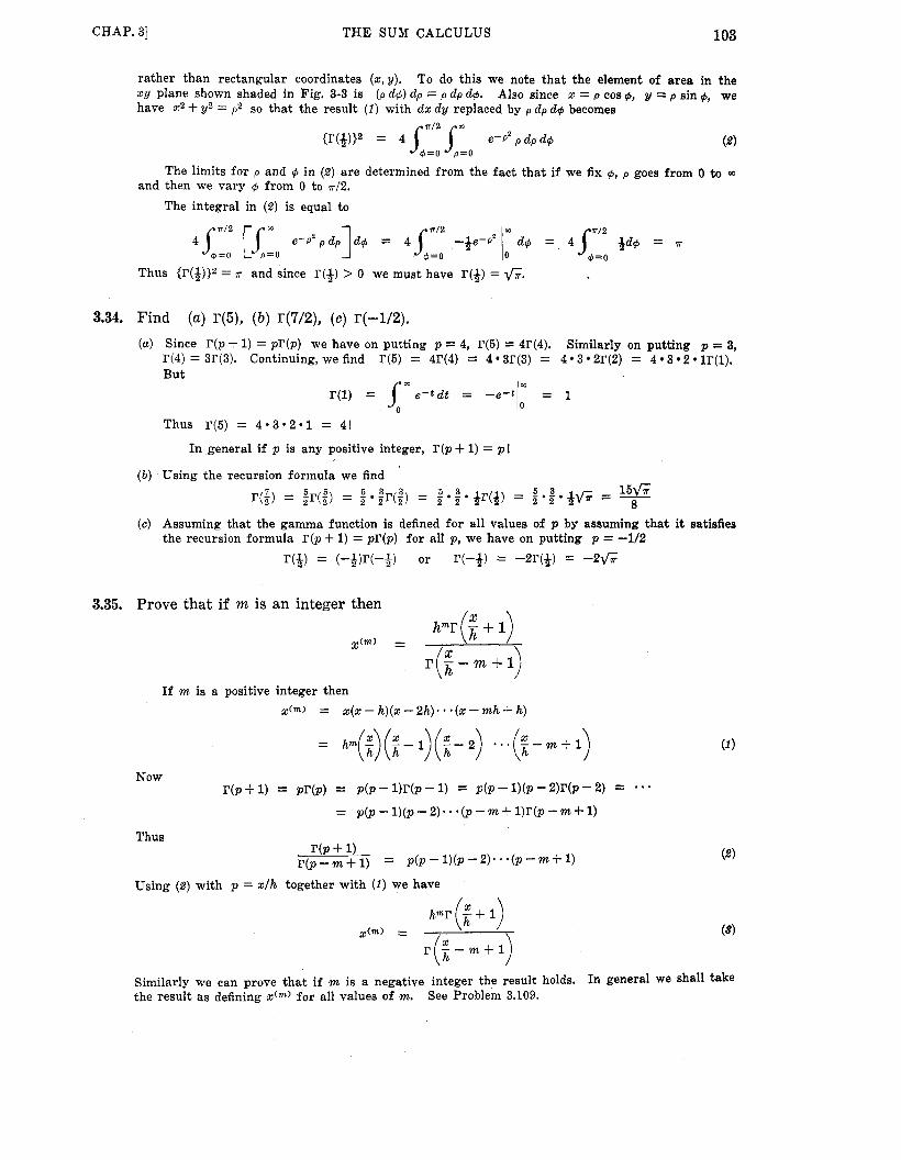
THE SUM CALCULUS 103 CHAP. 31
rather than rectangular coordinates (sly). xy plane shown shaded in Fig. 3-3 is (p dqj) dp = p dp d+. have x2 + y2 = p2 so that the result (1) with dx dy replaced by p dp d+ becomes
To do this we note that the element of area in the Also since x = p cos +f y = p sin +, we
{r(+)}2 = 4 sir'' Srn e - P 2 p dp d+ (2) @=0 p = o
The limits for p and qj in (2) are determined from the fact that if we fix +f p goes from 0 to m and then we vary qj from 0 t o ~ 1 2 .
The integral in (2) is equal to
Thus {r(+)}2 = n and since r(3) > 0 we must have r(4) = G.
3.34. Find (a) r(5), ( b ) r(7/2), (c) 1?(-1/2).
Since r (p + 1) = p r ( p ) we have on putting p = 4, r(5) = 4r(4). Similarly on putting p = 3, r(4) = 3r(3). Continuing, we find 135) = 4134) = 4 3133) = 4 3 2132) = 4 3 2 lr(1). But
r(1) = Jrn e- tdt = -e - t iw = 1 0 0
Thus r(5) = 4 . 3 . 2 . 1 = 4!
In general if p is any positive integer, r(p + 1) = p !
Using the recursion formula we find 7 5 5 5 3 3 1 5 6 +fi = - r(z) = z r ( p ) = zr(5) = :* :* +r(&) =
Assuming that the gamma function is defined for all values of p by assuming that i t satisfies the recursion formula r(p + 1) = pI'(p) for all p , we have on putting p = -1/2
r(&) = (-&)r(-+) or r(-+) = -2134) = -2fi
8
3.35. Prove that if m is an integer then hmr( i + 1)
r (i - m + I) %(m) =
If m is a positive integer then Z ( m ) = x(x - h)(x - 2h) * * * (x - mh + h)
= hm(;)(; - 1)( ;- 2) . . .(; - m + 1)
Now r(p+ 1) = p r ( p ) = p ( p - l ) r ( p - 1) = p ( p - l ) (p-2)r(p-2) = * * *
= p ( p - l ) ( p - 2)- ' ( p - m + l ) r ( p - m + 1)
Thus r(p + 1) (2)
p ( p - m+ 1) = P(P - 1)b - 2) . * '(P - m + 1)
Using (2) with p = x/h together with (1) we have
hmr (f + 1)
r ( ; - m + l )
See Problem 3.109.
x(m) = (3)
Similarly we can prove that if m is a negative integer the result holds. the result as defining drn) for all values of m.
In general we shall take
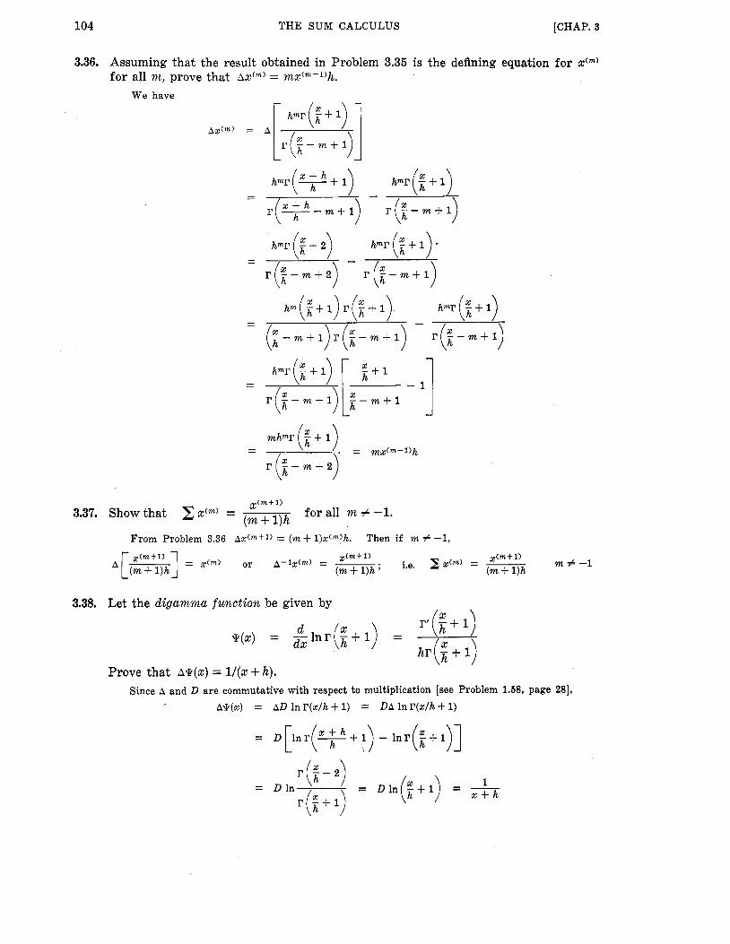
104 THE SUM CALCULUS [CHAP. 3
3.36. Assuming that the result obtained in Problem 3.35 is the defining equation for xCm) fo r all m, prove that Ax(m) = mx(m-l)h,
We have
X ( m + l ) for all m # -1. (m + 1)h 3.37. Show that Ex(") =
From Problem 3.36 A z ( m + l ) = (m -t l)xcm)h. Then if m # -1,
3.38. Let the digamma function be given by
h r ( i + 1) Prove that A q ( x ) = l/(x + h).
Since A and D a r e commutative with respect to multiplication [see Problem 1.58, page 281, A+(x) = AD In r (x /h + 1) = DA In r (x /h + 1)

CHAP. 31 THE SUM CALCULUS 105
1 r'(; + 1) 3.39. Prove that 2 x(-l) = x+h =
h r ( i + 1)'
From Problem 3.38 we have since - - - x(-l), x + h
A-1- 1 = A - 1 ~ ( - - 1 ) = *(z) = x + h
i.e.
BERNOULLI NUMBERS AND POLYNOMIALS 3.40. Prove that if fn(x) is a polynomial of degree n having the property that Dfn(Z) =
fn- l (x) , then fn(x) must have the form coxn c1xn-1
n! (n-l)! f n ( x ) = - + - + ' * * + Cn-1X + Cn
where CO, CI, . . . , cn are constants independent of n. Suppose that fn(x) = Ao(n)xn + Al(n)x*-l + * * + An-l(n)x + A,(n)
Then by using D f n ( x ) = fn-l(x) we have
nAo(n)xn-l + (n - l)A,(n)xn-2 + * * * + A,-,(n) = Ao(n - 1)xn-1 + A,(% - 1)xn-2 + - * * + An-l(n - 1)
Since this must be an identity, it follows that
%Ao(%) = Ao(n - l), (n - l)Al(n) = Al(n- l), . . ., An-l(n) = An-l(n- 1)
A,(% - 1) From the first of these we have
n A&) =
Then replacing n by n - 1 successively we find
AOP) - - CO - - A,@-2) - - ..I = - A,(% - 1) A,(%) = n n(n - 1) n(n - 1). * e l n!
where co = Ao(0) is a constant independent of n.
Similarly from the second we have
C1 (n - 1) !
- - A 1 h - 2 ) - A l(0) - - ... = - A l b - 1) A l W = n - 1 (n - l)(n - 2) (n - l ) (n - 2). * *1
where c1 = A,(O) is a constant independent of n. By proceeding in this manner the required result is obtained.
3.41. Find p,(x) for n = 0, 1,2,3. By definition [see (SO), page 86, with n=4] Ap4(x) = x3/3!. Thus with h = 1
A - 1 - 23 = -4-1x3 1 3! 3!

106 THE SUM CALCULUS [CHAP. 3
3.42. Obtain the Bernoulli polynomials B,(x) fo r 92 = 0,1,2,3. Since by definition B,(x) = n ! B,(x), we have using Problem 3.41
B ~ ( x ) = O ! B ~ ( x ) = 1
B ~ ( x ) = l! B,(x) = z - 3 B ~ ( x ) = 2 ! B ~ ( x ) = 2 2 - x + 6 B ~ ( x ) = 3! B,(x) = ~3 - 4x2 + QX
3.43. Obtain the Bernoulli numbers B, fo r n = 0, 1,2,3. Since by definition B, = B,(O), we obtain from Problem 3.42
Bo = 1, B1 = -4 , B2 = 4, B3 = 0
Prove that
where 5'; are the Stirling numbers of the second kind.
Use this result to solve Problems 3.41, 3.42 and 3.43.
From definition (SO), page 86, we have % n - l - 1 P,(x) = A - 1 - - - ~ - 1 $ n - l
(n - 1) ! (n - 1) ! Replacing n by n + 1 and using (31), page 7, with h = 1 we have
Putting n = 3 in the result of (a) we have
L
- - 1x3 - A 5 2 + &X in agreement with Problem 3.41. From these we can determine P 2 ( x ) , PI(%) and Po(%) as in that problem.
We can from these also determine the Bernoulli polynomials and Bernoulli numbers as in Problems 3.42 and 3.43.

CHAP. 31 THE SUM CALCULUS 107
3.45. (a) If
prove that for n = 2,3, . . .
( 6 ) If B n are the Bernoulli numbers prove that they must satisfy the recurrence formula (1 + B)" - Bn = 0 where, after formally expanding by the binomial theorem, Bk is replaced by B k .
Use ( b ) to obtain the first few Bernoulli numbers.
We have for n = 1,2 ,3 , . . . b&" blAXn--l
A P n ( 4 = - + * * * + b f l - lAs n! +-
Then putting x = 0 in ( I ) and using the fact that
AX" I x = o = [ ( x + - zn] I x = o = 1
b0 bl we find APn(0) = 7 + + + bf l - i
Also since
we have on putting x = 0 0 n = 2 , 3 , . . . 1 n = l APnW =
and the required result follows from ( 2 ) and (3).
The Bernoulli numbers are given by
B, = B,(O) = n! B,(O) = n! b,
Thus
where O! = 1.
Then using (4 ) in the result of part (a) we have
Multiplying by n! (5 ) becomes since Bo = 1
which is the same as expanding (1 + B)n- Bn = 0 formally and then replacing Bk by Bk.
Putting n = 2,3,4, . . . in (5) we find
I + ( Y ) B 1 + ( ; ) B 2 = 0, 1 + 3 B l + 3 B z = 0 or Bz = Q
l + ( ~ ) B 1 + ( ~ ) B ~ + ( ~ ) B 3 = 0 , 1 + 4 B l + 6 B z + 4 B 3 = 0 or B , = O
etc.

108 T H E SUM CALCULUS [CHAP. 3
3.46. Prove that for r = 1,2,3, . . . (n + B)'+l - Brtl
r + l 1' + 2' + 3' + . . . + (n-1)' =
where the right side is to be expanded formally using the binomial theorem and then replacing Bk by B k .
From equation (SO), page 86, we have on putting n = r + 1
Then using n = r + 1 in equation ( 3 4 , page 86, and property 1, page 87,
B,+,(s) - (x+B)++ ' r + l A-lx' = r ! P T t l ( x ) = ~ - r + l
Thus by the fundamental theorem of sum calculus,
n-1 (x + B ) (n + B)'+' - BVfl B x' = r + ;+'I: = r + l x=l
3.47. Use Problem 3.46 to evaluate l2 + 22 + 32 + . * . + n2. Putt ing r = 2 in the result of Problem 3.46 we have
(n + B)3 - B3
= Q ( n 3 + 3n2B1+ 3nB2 + B3 - B3) 3 1 2 + 2 2 + 3 2 + +(n-1)2 =
= $(n3 f 3n2B1 + h B 2 )
= in3 -+n2+ ln 6
= Qn(n - 1)(2n - 1) Then replacing n by n + 1 we have
12 + 22 + 32 + * * + n2 = Qn(n + 1 ) ( 2 n + 1) Note t h a t this agrees with the result of Problem 3.21(a).
EULER NUMBERS AND POLYNOMIALS 3.48. Show that the Euler polynomials are given by
where the constants eo, . . . , en are given for n = 1,2,3, . . . by
and eo = 1.
From Problem 3.40 and definition (38) on page 88 i t follows t h a t
Then using definition (39) on page 88 together with ( 1 ) i t is seen tha t we must have
Xn
n ! - e0 el -M(xn) + -M(xn-1) + + endlM(x) + en
n ! (n - 1) ! where M is the averaging operator with h = 1 which is a linear operator.

CHAP. 31 T H E SUM CALCULUS 109
If n = 0, ( 2 ) becomes
while (1) yields for n = 0
MEo(x) = 1 = eo
EOb) = eo
E ~ ( x ) = 1 We thus conclude from (3) and ( 4 ) t h a t
If n = 1,2 ,3 , . . . we have by definition of M
M ( x n ) = *[(X + 11% + Xn]
M(sn) Ix=o = 4 so tha t on putting x = 0
Thus on putting x = 0 in (2) we obtain for n = 1,2,3, . .
as required.
3.49. (a) Find eo,el,e2,e3 and ( b ) obtain the first four Euler polynomials.
(a) We already know from Problem 3.48 tha t eo = 1. result ( 6 ) of Problem 3.48 we have
Then putting n = 1,2,3 successively in the
From this we find el = -*, e2 = 0, e3 = 1 2 4
(b) Using par t (a) we obtain from (1) of Problem 3.48
x2 x 2 ! 2 E ~ ( x ) = - - -, X 3 X 2 1 E ~ ( x ) = - - - 3 ! 2 . 2 ! + 2 4
For a table of Euler polynomials see page 237.
3.50. Obtain the first four Euler numbers. By definition the Euler numbers given by
5 , = 2 n n ! E n ( 4 )
Then from the results of Problem 3.49(b) we have
Eo = 1, El =‘O, Ez = -1, E3 = 0
For a table of Euler numbers see page 236.
MISCELLANEOUS PROBLEMS 3.51. Prove that the generating function for the Bernoulli polynomials is given by
If we let G(x, t ) denote the generating function, then
using the fact tha t &(x) = n! P,(x).
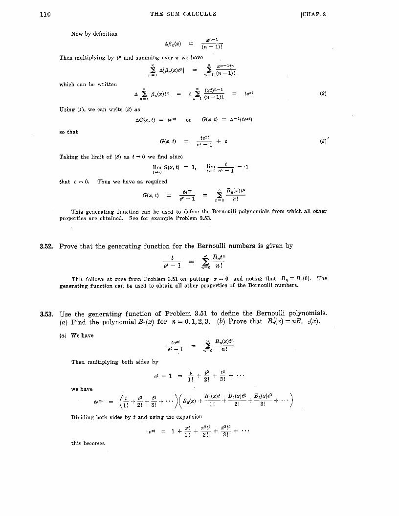
110 THE SUM CALCULUS [CHAP. 3
Now by definition Xn- l
APn(Z) = ~ (n - 1) !
Then multiplying by tn and summing over n we have
Using ( I ) , we can write (2 ) as
AG(x, t ) = text or G(x, t ) = A-'(teZt)
so that
+ o text G(x , t ) = - et - 1
Taking the limit of (3) as t + 0 we find since
lim G ( x , t ) = 1, lim - t * O t - r o et - 1
(3) '
that c = 0. Thus we have as required
This generating function can be used to define the Bernoulli polynomials from which all other properties are obtained. See for example Problem 3.53.
3.52. Prove that the generating function for the Bernoulli numbers is given by t = %--. Bntn
et - 1 n=O n!
This follows a t once from Problem 3.51 on putting x = 0 and noting that Bn = Bn(0). The generating function can be used to obtain all other properties of the Bernoulli numbers.
3.53. Use the generating function of Problem 3.51 to define the Bernoulli polynomials. (a) Find the polynomial Bn(x) for n = 0, 1,2,3.
(a) We have
( b ) Prove that BL(x) = nBn-i(x).
Then multiplying both sides by
we have
Dividing both sides by t and using the expansion
x t X * t Z X3t3 l! 2! 3!
ext = 1 + - + - + - + this becomes

CHAP. 31 THE SUM CALCULUS 111
1 + - xt + ~ X 2 t 2 + -+ X3t3 . * * = B o b ) + [ s + y ] t l ! 2 ! 3 !
Then equating coefficients of corresponding powers of t we have
From these we find
Bo(z) = 1, B , ( z ) = x - 4, B,(x) = x2 - x + 4, B3(X) = x3 - 8x2 + 42, * . .
Ib) Differentiating both sides of
with respect t o x we have t2e"t - 5 BA(x)tn - -
et - 1 n=O n !
But this is the same as Bn(x)tn Bh( x) t n = i--
t x T n=O n=O n !
i.e.
or
since BA(x) = 0. Equating coefficients of tn on both sides we thus find
Bn-l(x) - __ BA(4 - - (n - 1) ! n !
BA(x) = nBn-l(x) so that
3.54. Find 2 !%?E dx. X
We have by Leibnitz's rule on page 81
3 sina4 2 sina3 cos xa dx + ~ - -
- 4 sin a4 - 3 sin a3 - a

112 T H E SUM CALCULUS [CHAP. 3
Supplementary Problems THE INTEGRAL OPERATOR AND RULES OF INTEGRATION 3.55. Find each of the following:
(a) 0 - 1 ( 3 ~ 4 - 2x3 + x - 1) (c) 0-1(4 cos 3x - 2 sin 3%)
( b ) D - 1 ( 2 6 - - 3%) (d) 0-1(4e25 + 3e-4") (f) D - W )
3.56. Prove (a) formula 1-1 and ( b ) formula 1-2 on page 79.
3.57. Find (a) s ~ e - ~ z dx, ( b ) s (x sin x + cos x) dx, (c) s x In x dx, (d) x2 ln2x dx.
3.58. Find ( a ) s $2 sin2x d x , ( b ) f x3e2"dx.
3.59. Find
c
THE SUM OPERATOR AND RULES OF SUMMATION sin r (x - $h)
3.60. Prove tha t A- ' [cosrx ] = 2 C O S ~ = 2 sin +rh '
3.61. Use Problem 3.60 to obtain cos rx dx. S 3.62. Find A-l[xez] = z xe".
3.63. (a) Find A-1[x2ax] = z xzax, a # 1, and ( b ) check your answer.
3.64. Prove tha t
3.65. Find (a) c o s m ) , ( b ) A-'(x sinrx) .
DEFINITE SUMS AND THE FUNDAMENTAL THEOREM OF SUM CALCULUS 3.66. Evaluate each of the following using the fundamental theorem of sum calculus and verify directly.
(a) 2 2 d 4 ) if h = 2 (c) 2 cos 4x if h = r/3
( b ) [3x(2) - 2 x ( 3 ) ] if h = 1 (d ) 2 6 ~ ( - ~ ) if h = 4
8 71
2 0 4 10
1 2
n
1 3.67. Find 2 ~ ( - 3 ) if h = 1.
n
1 3.68. Find 2 x 0 2 ~ if h = 1.
a + ( n - l l h z x = a
3.69. Show t h a t $2 = na2 + +n(n - l)h(2a + h) + Qn(n - l)(n - 2)hz
DIFFERENTIATION AND INTEGRATION OF SUMS 3.70. Verify t h a t Theorem 3-3, page 84, is t rue for

CHAP. 31 THE SUM CALCULUS 113
3.71. Use Theorem 3-4, page 84, to obtain IV-7 from IV-6, page 83.
3.72. Find (a) x x COSTX ( b ) 2 x s inrx by using Theorem 3-4, page 84.
3.73. Prove (a) Theorem 3-3, (b) Theorem 3-4, (c) Theorem 3-5, on page 84.
SUMMATION OF SERIES 3.74. Sum the series (a) 1 + 2 + 3 + - * * to n terms, (b) 1 + 4 + 7 + 10 + * * to n terms.
3.75. Sum each of the following series to n terms.
(a) 1 . 2 + 2 . 3 + 3 . 4 + . * * (c) 1 .3 + 3 . 5 + 5 . 7 + (b) 1 . 2 0 3 + 2 . 3 0 4 + 3 0 4 . 5 + * a * (d ) 2 . 5 3- 5 . 8 + 8.11 + * * a
3.76. Sum each of the following series to n terms.
1 + ... 1 +- (') 1.4.7 4 * 7 * 1 0 + 7 * 1 0 * 1 3
1 1 1 1
1 1 1 1 1
(a) =+-+-+ * * * 2 . 3 3 . 4
(d ) i-& + - + -+ * " ( b ) E+E+fi+ ..' 2 - 3 . 4 3 . 4 0 5
n + 2 and thus ( b ) show that 3.77. (a) Show that x - = 2 - - n k k = l zk 2n
= 2 - + - + - + - + . . . 1 2 3 4 2 22 23 24
3.78. Find the sum of the series 1 * 2 l + 2-22 + 3 29 + 4.24 + + n*2n.
cos (e/2) - cos (n + #e 2 sin (e/2)
3.79. Show that sin e + sin 2e + sin 36 + - * + sin n6 =
nz(n + 1 ) 2
4 3.80. Show that 13 + 23 + 33 + * + n3 = (1 + 2 + 3 + - - - + n)2 =
3.81. Find the sum to infinity of each of the series in Problem 3.76.
3.82. Sum the series 1 22 + 2 32 + 3 42 + * * to n terms.
n
k = l 3.83. Sum the series x k2 Zk.
3.84. Sum the series 1 2 + 32 + 52 + - * - to n terms.
to n terms 10 3.85. (a) Sum the series
7 +- 4 +-+-+. ' " 1 - 2 . 3 2 . 3 0 4 3 . 4 0 5 4 0 5 . 6
and ( b ) find the limit a s n += m.
3.86. Sum each of the following series to n terms and to infinitely many terms. 1 1 1 1 1 1 +-+ -+* . .
2.4.6 3 . 5 . 7 5 . 7 0 9 (a) - + - + - + 2 - 4 3 ' 5 5 ' 7 . ' .
SUMMATION USING SUBSCRIPT NOTATION 3.87.
3.88.
Use the subscript notation to sum the series of Problem 3.75.
Use the subscript notation to sum the series of Problem 3.76.

114 THE SUM CALCULUS [CHAP. 3
n
k = l 3.89. Sum the series k*(k + 1).
3.90. Sum the series 2 k - 1 k Z 1 ( k + 2)(k + 4)
W 2k - 1 ( b ) k?1 ( k + l ) (k + 2)(k + 3) *
3.91. Sum the following series to n terms.
( a ) 1 . 3 - 5 - 7 + 3 - 5 - 7 . 9 + 5 * 7 * 9 * 1 1 + ... 1 + ... 1 1
1 . 3 . 5 . 7 + 3 * 5 * 7 * 9 + 5 - 7 * 9 . 1 1
3.92. Show tha t
a Z 1 (a) kak = ( n + l ) a n + l - an+2 - a k=O a - 1 ( a - 1)2
3.93. Sum the series + * 6 + - + - 1 ' 3 . 5 3 . 5 0 7 5 ' 7 ' 9 (a) to n terms.
( b ) to infinity.
ABEL'S TRANSFORMATION 3.94. " k Use Abel's transformation to sum the series kzl 5.
n
k=l 3.95. Sum the series k2 by using Abel's transformation.
n
k=l 3.96. Sum the series 2 k2ak' a f 1, by using Abel's transformation.
OPERATOR METHODS OF SUMMATION 3.97.
3.98.
3.99.
3.100.
3.101.
Work Problem 3.92 by using the result of Problem 3.30.
Show t h a t rk+l sin a(k - 1) - r k sin ak
r2 - 2r cosa + 1
rk+l cos a(k - 1) - y k cos ak
A- l [ rk sin ak] =
A-l[rk cos ak] = r2 - 2r cos a + 1
Problem 3.98 to show tha t if jr/ < 1 r sin a
r2 - 2r cos a + 1
1 - r2 2(r2 - 2r cos a + 1)
5 r k s inak = k=l
?'+ 5 r k c o s a k = 2 k=l
Show t h a t if p # 1 is a constant and h # 1,
thus generalizing the result of Problem 3.30.
Use Problem 3.100 to find A-l[xaz] . Compare with Problem 3.16.

CHAP. 31 T H E SUM CALCULUS 115
THE GAMMA FUNCTION 3.102. Find (a) I’(4), jb ) r(5/2), (c) r(-5/2).
3.103. Evaluate
3.104. Evaluate
3.105. Evaluate
3.106. Prove tha t
3.107. Prove t h a t
im xe-x3 dx.
A’ x2 ln2 x dx.
3.108. Use Problem 3.107 to express in terms of gamma functions
1 1 1 (X+1)2 + + * I ’ + - (x + n)2
and generalize.
3.109. Show tha t equation (3) of Problem 3.35 holds for all values of I n .
BERNOULLI NUMBERS AND POLYNOMIALS 3.110. ( a ) Find &(x) for n = 4 and 5 and thus obtain ( b ) the Bernoulli polynomials and (c) the Ber-
noulli numbers for n = 4 and 5. ’
3.111. Obtain the Bernoulli numbers B4, B6, BB without first finding the Bernoulli polynomials.
3.112. Prove t h a t B i ( x ) = nB,-,(x) without using the generating function.
3.113. Prove t h a t B, = B,(O) = B,(l).
3.114. Evaluate ( a ) 13 + 23 + 33 + * * - + 123, ( b ) 1 4 + 24 + 34 + * * * + n4.
3.115. Expand 5x4 - 8x3 + 3x2 - 4x + 5 in a series of Bernoulli polynomials.
1 n=O 3.117. Prove t h a t i l B n ( X ) d X = { 0 n > O ’
3.118. Prove t h a t 132,+1(+) = 0.
EULER NUMBERS AND POLYNOMIALS 3.119. Find ( a ) e4, e,; ( b ) E 4 ( x ) , E&); (c) E,, E,.
4.120. Prove t h a t (a) E,(O) = en, ( b ) E,(O) + E,(1) = 0, (c) E,(1) = -en*
17 -31 3.121. Show t h a t (a) e7 = - 40,320 ’ ( b ) = 362,880 *
MISCELLANEOUS PROBLEMS 3.122. Determine whether the operators (a) D and D-1, ( b ) A and A - 1 are commutative.

116 THE SUM CALCULUS [CHAP. 3
3.123. Prove that sin (PX + q - +ph - 4%)
2 sin Bph (a) A - l sin(pz + q) =
cos (PX + 4 - Jph - -&T)
2 sin -$ph ( b ) A-1 cos(px+ q) =
3.125. Use Problem 3.124 to find A-l[x3 2x] if h = 1.
n
k = l 3.126. Find 2 k3 cos2k.
- 1 2 ~ 22'4 ~ 32'42 I ... + n2.4n-1 1 (?~-1)4" ( n + l ) ( n + 2 ) = s + x-n- 3.127. Show that 2 . 3 3.4 4 ,
3.128. Show that if sin (Y # 0 n 2 2 sin (I
sin na cos (n + 1 ) ( ~ sin2a + sin22a + - . . + sinzna = - -
( a W - 2an2 - 2an + n2 + 2n + a + l ) a n + l - ( a2 + a ) (a - 1)s 3.129. Show that $ W * a k =
k = l
3.130. Prove that
3.131. Use Problem 3.130 t o show that
3.132. Evaluate 1 5 + 25 + 35 + - * - + 725. 3.133. Show that
1 1 1 1 + - + - + - + 9 * t o n terms = sin B s m 2 e sin 4e sin88 cot (e/2) - cot 2n-le
sec2x tan h = tan + c. 1 3.134. (a) Show that A-l[ - tan tan
( b ) Use (a) to deduce that sec2x dx = tan x + c. S 3.135. (a) Show that = tan-' s + c.
( b ) Use (a) to

CHAP. 31 THE SUM CALCULUS 117
3.136. ( a ) Show that
k=l 5 tan-1 (kZ + ‘k + 1)
3.137. Are there any theorems for integrals corresponding to the Theorems 3-3, 3-4 and 3-5 on page 84? Explain.
3.138. (a) Show that formally -(1+ E + E 2 + * * * ) 1 A-1 = = -- -
A 1 - E - ( b ) Use (a) t o obtain the formal result
A-l f ( x ) = - f(u) u=x
where the sum on the right is taken for u = x, x + h , x + 2 h , . . . . (0) Is the result in (b ) valid? Illustrate by considering the case where f ( x ) = ___ with h = 2 . x ( x + 2)
3.139. Prove Theorem 3-1, page 83.
3.140. Prove ( a ) Theorem 3-3 and ( 6 ) Theorem 3-4, page 84.
G(a + A @ ) - G(a) ha
b ( a ) [Hin t . Let G(a) = i(al F(x, a) d x and consider
3.141. Prove that I?’@) = J a e--5 In x d x = -y where y is Euler’s constant [see page 851. 0
3.142. Use Problem 3.141 t o prove that
+ Y 1 1 1 r’(n + 1)
n r (n + 1) I+,+,+ . . . + - = ____
3.143. Supply a proof of the method of generalized integration by parts [see Problem 3.41.
3.144. The beta funct ion is defined as
( a ) Show that B(m, n) = 2
( b ) Show that B(m, n) = B(n, m).
3.145. Show that the beta function of Problem 3.144 is related to the gamma function by
w w
[Hint.
transform to polar coordinates and use the result of Problem 3.144.1
Use Problem 3.106 t o show that r (m) r(n) = 4 1 x2~- l y2n-1e -~x2 tY21 dx dy. Then 0 0
3.146. Evaluate ( a ) i’ *dyl ( b ) Jn/2sin4e 0 cos2e ds , (c) &7’zG de.
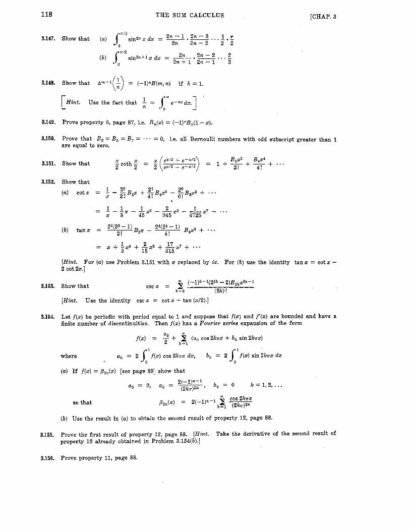
118 THE SUM CALCULUS [CHAP. 3
3.148. Show that A m - l ( i ) = (-l)nB(m,n) if h = 1.
Hint. Use the fact that I. = 1% e-nsdx.] ' c n
3.149. Prove property 6, page 87, i.e. B,(x) = (-l)nBn(l - x).
3.150. Prove that B3 = B5 = B7 = = 0, i.e. all Bernoulli numbers with odd subscript greater than 1 are equal to zero.
5 X ex12 + e - x / 2 B ~ x ' B4~4 -coth- = g ( 2 2 2 e x / 2 - e-x/2 2! 4!
) = 1 + - - + - + ... 3.151. Show that
3.152. Show that 22 24 26
x 2! 4! 6! (a) cotx = - - -B2x + -B4x3 - -B6x5 + ...
1 $7 - ... 1 2 x - - - - - x - - x 3 - - 1 1 5 - -
4725 x 3 45 945
22(22 - 1) 24(24 - 1) BqX3 + . . . 4! ( b ) t a n s = 2! B ~ x -
= x + -x3 1 + -x5 2 + -x7 17 + ... 3 15 315
[Hint. For (a) use Problem 3.151 with E replaced by ix. For ( b ) use the identity tan x = cot x - 2 cot ex.]
3.153. Show that (-1)k-l(22k - 2)B x2k-1
2k cscx = i k = O (2k) !
[Hint. Use the identity csc x = cot x + tan (x/2).]
3.154. Let f(x) be periodic with period equal to 1 and suppose that f(x) and f'(x) are bounded and have a finite number of discontinuities. Then f(x) has a Fourier series expansion of the form
f(X) = ao + (Uk COS2knx + b k Sin2kn-X) 2 k = l
1 where a k = 2 f(X) COS2knX dX, bk = 2 J1f(E) S in2kT~ dX
(a) If f(x) = PZn(x) [see page 881 show that
b k = 0 k = 1 , 2 , ... 2(-1)n-1 (2kn)Zn ' a,, = 0, a k =
so that
(b) Use the result in (a) to obtain the second result of property 12, page 88.
3.155. Prove the first result of property 12, page 88. property 12 already obtained in Problem 3.154(b).]
[Hint. Take the derivative of the second result of
3.156. Prove property 11, page 88.

CHAP. 31 T H E SUM CALCULUS 119
3.157.
3.158.
3.159.
3.160.
3.161.
3.162.
3.163.
3.164.
3.165.
3.166.
3.167.
3.168.
3.169.
3.170.
3.171.
Show tha t - 1 1 1 772 12+$+s+ ' . * = -
( b ) -+-+t34+ * . . = -
6
1 1 1 774
1 4 24 90
772 12 - I + - - -+ . . . 1 1 = Show tha t ( a ) - - -
1 2 22 32 4 2
1 1 1 1 7774 ( b ) - - -+ - - -+ ... = - 1 4 24 34 44 720
7 3 1 1 1 1 - - 32 53 73
1 1 1 1 5775 (6) -- -+ -- -+ . . . - - 1 5 35 55 7 5 - 1536
- 13 33 + - - -+ * * * Show tha t ( a ) - - -
Prove (a) property 4 and (a) property 6 on page 88 by using the generating function.
Show t h a t B,(&) =
Show t h a t the Bernoulli numbers can be found from 2 (-l)kk!
k + l " B, = k = l
where S; a r e Stirling numbers of the second kind.
Use the result in (a) to obtain the first few Bernoulli numbers.
Prove tha t I n x - - - - - - - ... - (a) In s inx = - ... O < x < n
x2 x4 x6 (-1)k-'B2k(2%)2k 6 180 2835 2k(2k)!
772 774 Prove tha t 1 - -B2 + -B4 - * . * = 0. 2! 4 !
cc 32,-1 Prove t h a t B, = 4 n l m d x .
Prove that - ... (22k - 1)B2k$2k-1 - .. . - (24 - 1 1 ~ ~ x 3
(2k) ! - 1 (22- 1)Bzx
ex + 1 2 2! 4 ! - - 1 - _ -
1 1 1 Hint. - e2x - 1 = 2 (- e x - 1 - -).I e x + 1
Prove t h a t the only zeros of the polynomial B,,(x) - B2, in the interval and x = 1. .
(a) Obtain the generating function 8, page 89, for the Euler polynomials and ( b ) use i t to find the first four polynomials.
(a) Obtain the generating function for the Euler numbers and ( b ) use i t to find the first four numbers.
0 S x 5 1 a r e x = 0
Prove properties (a) 3 ( b ) 6 (c ) 7 on page 88.
Prove formulas (a) 9 (b) 10 on page 89.

120 THE SUM CALCULUS
3.172. Derive the results 12 on page 89.
3.173. Obtain property 11 on page 89.
3.174. (a) Show that
[CHAP. 3
where S t are Stirling numbers of the second kind.
( b ) Use (a ) to obtain a relationship between the Euler and Stirling numbers and from this find the first four Euler numbers.
- - 1 - i{Eo(r3) + E,(O)x + E,(O)xZ + a ' * } ex + 1 3.175. (a) Prove that
( b ) Use part (a) and Problem 3.166 to show that - 2 ( 2 * k - l)&
EO(O) = 1, E 2 k ( 0 ) = 0, EZk- l (O) = (2k.i k = 1 , 2 , . .
3.176. (a) Show that the first few t angen t numbers [see page 891 are given by
TI = I, T2 = 0, T, = 2, T, = 0, T, = 16, T, = 0, T, = 272, T, = 0, TB = 7936
( b ) Use (a) to show that 5 3 x5 X7 x9
t a n x = x + 2 . g + 16.- + 2 7 2 . 5 + 7936.91 + 9 . . 5!
Y
Applications the Sum Calc
SOME SPECIAL METHODS FOR EXACT SUMMATION OF SERIES In Chapter 3 we saw how the fundamental theorem of the sum calculus could be
used to find the exact sum of certain series. We shall consider, in the following, various special methods which can be used in the exact summation of series.
SERIES OF CONSTANTS Suppose the series to be summed is
In particular the series can be summed exactly if uk is any polynomial in k. See Problems 4.1 and 4.2.
POWER SERIES A power series in x is defined as a series having the form
Suppose that in this series we can write a k = U k v k where Uk can be written as a polynomial in k and where z)k is such that
v(X) = 2 z ) k X k ( 4 ) k=O
i.e. the series on the right of (4) can be summedexactly to V(X) . Then we can show that [see Problem 4.31
3 a k X k = V(XE)Uo = V(X + XA)UO k=O
A2Uo 3- * * * (5) x*V”(x)
= V(X)Uo + --j-j- 2 !
where primes denote derivatives of V(X) . right of (5) terminates and yields the exact sum of the series on the left.
Since Uk is a polynomial, the series on the
The following are some special cases. sc
I. z)k = 1. In this case V ( X ) = c xk = - and we find that k = O 1 - X
x4uo + X2A2uo + . . uo + ~ - - 1 - x ( 1 - x ) ~ ( 1 - ~ ) 3 = 5 U k X k
k=O 2 a k X k
k=O
This is sometimes called Montmort’s formula.
121

122 APPLICATIONS O F THE SUM CALCULUS [CHAP. 4
* X k 2. V k = U k ! . In this case V ( X ) = - = ex and we find that k=O k !
Note that we take O! = 1 by definition. For other special cases see Problems 4.37 and 4.47.
The power series method can also be used to sum various series of constants by letting x be equal to particular constants. See for example Problems 4.6 and 4.8.
APPROXIMATE INTEGRATION Finite difference methods are valuable in obtaining formulas from which we can com-
pute the aproximate value of a definite integral. One important method uses the Gregory- Newton formula [page 91 and yields the result [Problem 4.91
n(6n3 - 45n2 + llOn - 90) A”@) + 9 . .] 120 a3f(a) +
(8) The following are some important special cases.
I‘
h 1. Trapezoidal rule.
f ( x ) d x = 2 [f (a) + f(a + h)1 ( 9 )
This is obtained by letting n = 1 and neglecting differences of order 2 and higher
By using (9) repeatedly we can arrive at the extended trapezoidal rule [see Problem 4.101.
which holds for any positive integer N . If we let 76k = f(a + kh) denote the ordinates, (10) can be written as
2. Simpson’s one-third rule.
This is obtained by letting n = 2 and neglecting differences of order 4 and higher. See Problem
By using (12) repeatedly we can arrive a t the extended Simpson’s one-third rule
It is of interest that third order differences do not enter in this case. 4.13.
which holds for any even positive integer N . In ordinate notation (13 ) can be written as
(14) h latNh f ( X ) d% = - 3 [yo + 4Yi + 232 + 4Ys -k * * * f 4Yiv-1 -k Y N ]

CHAP. 41 APPLICATIONS OF THE SUM CALCULUS
Name of rule
Trapezoidal
123
Error term
h3
12 - - f ” ( [ ) , [ between a and a + h
3.
4.
Simpson’s three-eighths rule.
This is obtained by letting n = 3 and neglecting differences of order 4 and higher. See Problem 4.16.
By using (15) repeatedly we can arrive a t an extended Simpson’s three-eighths rule.
Weddle’s rule,
+ 5 { f ( a + h) + f(a + 5h)) + 6 f ( a + 3h)l (16) which can also be written as
f(x) d x 3h a + 6 h
= 10 [(YO + YZ + Y4 + YS) + ~(YI + 95) f 6 ~ 3 1 (17)
This is obtained by letting n = 6 and replacing the coefficient 41/140 of asf(a) by 42/140 = 3/10 and neglecting differences of order 7 and higher.
By using (16) or (17) repeatedly we can arrive a t an extended Weddle’s rule [see Problem 4.911.
In practice to obtain an approximate value for the definite integral
See Problem 4.38.
(18)
we subdivide the interval from a to b into N subintervals where N is some appropriate positive integer and then use one of the above rules.
ERROR TERMS IN APPROXIMATE INTEGRATION FORMULAS If we let Ii denote the error term to be added to the right hand side of any of the
approximate integration formulas given above, then we can find 5Y in terms of h and the derivatives of f ( x ) . The results are given in the following table.
Simpson’s one-third [ between a and a + 2h I I Simpson’s three-eighths 3h5 f ( * V ) ( [ ) , 5 between a and a + 3h I
-~ [h4ei(a) + E - f ( 8 ) ( [ ) ] , E between a and a + 6h 140 1400 Weddle’s
For a specified value of h it is in general true that Simpson’s one-third rule and Wed- dle’s rule lead to greatest accuracy followed in order of decreasing accuracy by Simpson’s three-eighths rule and trapezoidal rule.

124 APPLICATIONS OF THE SUM CALCULUS
GREGORY’S FORMULA FOR APPROXIMATE INTEGRATION We can express a definite integral in operator form as
[CHAP. 4
(See Problem 4.20.) By using this we obtain Gregory’s formula f o r approximate inteyra- tion given by
h a+nh
f(z) dx = 2 [yo i- 2Y1+ 2y2 + * + 2yn-1+ yn]
where the ordinates are given by zjk = f(a + kh) , k = 0, 1, . . . , n, and where V = A E - ~ is the backward difference operator [see page 91. In practice the series is terminated a t or be- fore terms involving the nth differences so that ordinates outside the range of integration are not involved. See Problem 4.23.
THE EULER-MACLAURIN FORMULA The Euler-Maclaurin formula , which is one of the most important formulas of the cal-
The culus of finite differences, provides a relationship connecting series and integrals. formula states that
1 n--1
k = O C f ( a + kh) = f ( x ) d x - 3 [ f (a + nh) - f(a)]
+ - h [?(a + nh) - ?(a)] - wo h3 [?”(a + nh) - ?”(a)] 12
and in this form is useful in evaluation of series involving f(x) when the integral of f ( x ) can be found.
Conversely the formula provides an approximate method for evaluating definite in- tegrals in the form
h a + n h
S, f ( x ) d x = 3 [yo + 2y1+ 2y2 + * * * + 2yn-1+ yn]
I - h2 [y! - y;] + - h4 [y;’ - YY’] 720 12
where we have used the notation !/k = f(a + kh), 2 ~ 6 = f’(a), U! = f’(a +nh), etc.
derivatives [see Problem 4.1011. We can also express the Euler-Maclaurin formula in terms of differences rather than
ERROR TERM IN EULER-RIIACLAURIN FORMULA
and polynomials including an expression for the remainder or error term. It is possible to express the Euler-Maclaurin formula in terms of Bernoulli numbers

CHAP. 41 APPLICATIONS O F THE SUM CALCULUS
To do this we first show that
125
Then replacing a by a + h, a + 2h, , . . , a + (n - l ) h and adding, we obtain the Euler-Mac- laurin formula with a remainder given by
l Q " ' f ( x ) d x = - h [ f ( a ) + 2 f ( a + h) + . + 2 f ( a + nh - h) + f ( a + nh)] 2
(24 m-l Bzph2p [f(Zp-l)(a + nh) - f ( Z ~ - l ) ( a ) ] + R - z1 rn
where the remainder R is given by
This can be used in connection with evaluation of series by writing it as
The result (26) is of course equivalent to (21) except that the error term R has been introduced.
STIRLING'S FORMULA FOR n !
is that for n ! , called Stirling's formula and given by An important formula which can be obtained by using the Euler-Maclaurin formula
When n is not an integer the result can also be used if the left side is replaced by the gamma function r (n + 1) [see page 851. The series in (27) is an asymptotic series and is useful for large values of n [actually there is good accuracy even if n = 10 as shown in Problem 4.781.

126
0
1
2
3
4
1
APPLICATIONS O F THE SUM CALCULUS
Solved Problems
1 3
4 2 5 0
9 2 0 7 0
16 2 9
25
[CHAP. 4
SERIES OF CONSTANTS 4.1. Prove that
A2Uo 4- ". n(n - l)(n - 2) 3 ! AUo 4- n(n - 1)
Uo + u1 + uz + * . * + Un-1 = nu0 + 2 !
We have from the definition of the operator E = 1 + A
UO + ~1 + ~2 + . * * + un-l = U O + Euo + E*uO + * . * + En-1~0
= ( 1 + E + E 2 + *.*+En-l)uo
En - 1 - - - E - l U o (1 + A)n - 1
A UO - -
4.2.
A*UO + ' ' I n(n - l)(n - 2)
3! Auo 4- n(n - 1) = nuo +
Sum the series l2 + 22 + 32 + * - . to n terms. Comparing with the series of Problem 4.1 we have
uo = 12, u1 = 22, u2 = 32, . . ., u,-~ = n2
Then we can set up the following difference table.
Fig. 4-1
It is clear from this table that
uo = 1, Auo = 3, A%, = 2, A3u0 = 0, A4u0 = 0, . . . 'I
which we could also obtain by observing that u k = ( k + Auk = 2k + 3, A2uk = 2 and putting k = 0.
, Thus using Problem 4.1 the required sum is
n(n + 1)(2n + 1) - - 6
in agreement with Problem 3.21(a), page 98.
as a polynomial in k so that differences are ultimately zero. Note that the method of Problem 4.1 is especially useful when the kth term can be expressed

CHAP. 41 APPLICATIONS O F THE SUM CALCULUS 127
POWER SERIES
= V ( X + X A ) U o
where we have used the Taylor series expansion
V ( x + h) with h = xA,
Note that although the above has been proved without any restriction on u k an important case where the series can be summed exactly occurs when u k is a polynomial in k so that higher differences are ultimately zero.
Put wk = 1 in the results of Problem 4.3. Then
Thus
m
1 + x + 2 2 + 2 3 + * ’ 1
1 - x , . = -
and so from Problem 4.3 we have
m
4.5. Sum the series ( k + l ) ( k + 2)xk = 1 .2 + 2.3% + 3 *4x2 + - . * . k=O
Comparing with Problem 4.4 we have u k = (k + l)(k + 2). Then we can construct the follow- ing difference table.

128 APPLICATIONS O F T H E SUM CALCULUS [CHAP. 4
I I Fig. 4-2
From this table i t i s clear tha t
uo = 2, Auo = 4, A2uo = 2, A3zt0 = 0, A4u0 = 0, . . . These could also have been obtained by letting k = 0 in the results z6k = ( k + l ) ( k + 2), A u k = 2k f 4, A2Uk = 2, . . . .
Thus we have from Problem 4.4 m 4x 2x2 3 ( k t 1 ) ( k + 2 ) x k =
k = O
2(1 - x ) ~ f 4 ~ ( 1 - X) + 2 x 2 - - (1 - x)3
2 ___ - - (1 - x)3
It should be noted t h a t the series converges only if !xi < 1.
2 . 3 3 . 4 4 . 5 5 . 6 4.6. Sum the series 1 . 2 - - + 7 - - 5 3 i-54 - . * * . 5 5
This series is a special case of the series of ProbIem 4.5 in which we let x = -1/5. Then the sum of the series i s
4.7. Prove that
1 P u t 2ik = l / k ! in the results of Problem 4.3. Then
Thus V'(x) = e x , V"(x) = ex, . . .
and so from Problem 4.3 we haxie

CHAP. 41 APPLICATIONS O F T H E SUM CALCULUS 129
+ * . . 5 2 82 1 1 2 4.8. Sum the series 2 2 + - + + - 1 ! 4 2 ! 4 - 3!43
The series is a special case with x = 114 of
11' 3!
5 2 82 l! 2! 22 + - x + - 2 9 + --3 + . . -
or
Thus we can obtain the sum by putting u k = (3k+2)2 in the result of Problem 4.7. difference table i n Fig. 4-3 we find
From the
uo = 4, Auo = 21, A2uo = 18, A3u0 = 0, . ..
21 25 18
39 0
57 0 64 18
121 18 75
196
Fig. 4-3
Thus
and putting x = 114 the required sum is seen to be 157&16.
APPROXIMATE INTEGRATION 4.9. Prove that
A2f ( a ) n(2n - 3 )
n(n - 2)2 n(6n3 - 45n2 + 110n - 90) A 4 f ( 4 + . * .] + 24 A3ff(a) + 120
By the Gregory-Newton formula (44) on page 9 we have
Using Ax = h and the definition of ( z - this can be written
f ( z ) = f (a) + ? ( x - a ) + - A s f ( a ) ( x - a)(% - a - h) 2 ! hz
A3f(a)(x - a ) ( x -a - h)(x - a - 2h) + . . . 3! h 3 + -~
Integrating from x = a to a + nh we then have

130 APPLICATIONS O F THE SUM CALCULUS [CHAP. 4
+- ~ / ~ ) ~ a t " h ( x - a ) ( x - a - h ) ( x - a - 2 h ) ( x - u - 3 h ) d x +
A 4 f ( a ) + * n(n - 2)2 ~ ( 6 ~ 3 - 4 5 ~ 2 + 110% - 90)
+ ,,A3f(a) + 120
4.10. Prove the trapezoidal ru le
Put n = 1 in the result of Problem 4.9. Then assuming that differences of order higher than two are zero we have lath fb) dx = h [ f ( a ) + ?pV(a)I
= h [ f ( a ) + &{f (a + h) - f(a)}I
5 [fb) + f ( a + h)] h =
4.11. Use Problem 4.10 to obtain the ex tended trapezoidal ru l e
From the results of Problem 4.10 we have
It = 5 [!(a + h) + f(a + 2h)]
............................................... h z [ f ( a + ( N - 1)h) + f ( a +- Nh)]
a t N h
f ( x ) d x = a t ( N - 1 ) h
Then by addition
h 2 l a t N b f ( x ) d x = - [ f ( a ) + 2 f ( a + h) + - * * + 2f (a + ( N - 1)h) + f ( a + Nh)!
or using ordinates ?dk = f ( a + kh),
1
4.12. (a) F i n d l d x by the extended trapezoidal rule where the interval of integration
is subdivided into 6 equal parts. ( b ) Compare the result. with the exact value. (a) We have a = 0, a + N h = 1 so that since N = 6 , h = 1/6. The work of computation can be
arranged in the following table.

CHAP. 41 APPLICATIONS O F THE SUM CALCULUS 131
x 0
f ( x ) = 1/(1+ 6) 1.00000000
116 216 316 416 516 1
0.97297297 0.90000000 0.80000000 0.69230769 0.59016393 0.50000000
Then applying the extended trapezoidal rule of Problem 4.11 we have
i* = 3 11 + 2(0.97297297 + 0.90000000 4- 0.80000000 + 0.69230769 + 0.59016393) 1 + x2 2 + 0.50000000]
= 0.78424077
( b ) The exact value is 1 dx i1 i-j-~ = tan-1% = t a n - l l = 4 = 0.785398163.. ,
10
Thus the trapezoidal rule for this number of subdivisions yields a result which is accurate t o two decimal places. The percent error is 0.147%.
4.13. Prove Simpson’s one-third rule
Put n = 2 in the result of Problem 4.9. Then assuming that differences of order 4 and higher are zero we obtain
f ( x ) dx = 2h[f(a) + Af(a) + &A2f(a)] = 2h[f(a) + { f ( a + h) - f(a)> + + 2h) - 2 f b + h) + f(a)>l
l‘+zh = [ f ( a ) + 4f(a + h) + f ( a + 2h)] 3
4.14. Use Problem 4.13 t o obtain the extended Simpson’s one-third rule
where it is assumed that N is even. From the results of Problem 4.13 we have
J ‘ + z h f ( m ) dx = 4 [f(a) + 4f(a + h) + f ( a + 241
h J-==;; f(x) dx = j- [ f ( a + 2h) + 4f(a + 3h) + f ( a + 4h)]
............................................. .................... h a + NIL
f(x) dx = 3 [ f ( a + (N - 2)h) + 4f(a + (N - 1)h) + f ( a + WI S a f ( N - 2 ) h
Then by addition
f(x) dx = [ f (a) + 4f(a + h) + 2f(a + 2h) + 4f(a + 3h) + * * + f ( a Nh)] J-=,+,, Using ordinates yk = f ( a + kh) this can be written
h 3 f(z) dz = - [yo + 4Y1+ 2y2 + 4u3 + - . . + ~ Y N - I + YNI

132 APPLICATIONS OF THE SUM CALCULUS [CHAP. 4
4.15. (a) Work Problem 4.12 by using the extended Simpson’s one-third rule and ( b ) com- pare your result with the exact value and that obtained from the trapezoidal rule. (a) We can apply the rule since N = 6 [which is a multiple of 31. It is convenient to write the
rule in the form
= [ l .OOOOOOOO + 0.50000000 + 4(0.97297297 + 0.80000000 + 0.59016393)
+ 2(0.90000000 + 0.69230769)l 3
= 0.78539794 where we have used the value h = 1/6 and the table of values obtained in Problem 4.12 which is applicable here.
( b ) The result is seen to be accurate to 6 decimal places on comparison with the exact value 0.78539816.. , as obtained in Problem 4.12(b). The percent error is 0.00028%. It is clear that the result is f a r more accurate than that obtained using the trapezoidal rule.
4.16. Prove Simpson’s three-eighths rule
Jat3hf(z)dz = [ f ( a ) + 3f(a + h) + 3f(a + 2h) + f ( a + 3h)]
Put n = 3 in Problem 4.9 and neglect differences of order 4 and higher. Then a t 3 h
f ( x ) dx = 3h [ f ( u ) + %Af(a) + fA2f(a) + &Asf(a)]
= 3h [f(a) + $Cf(a + h) - f ( a ) > + f { f ( a + 2h) - 2f(a + h) + f (41 + & { f ( a + 3h) - 3f(a + 2h) + 3f(a + h) - f(a)>]
[f(a) + 3f(a + h) + 3f(a + 2h) + f ( a + 3h)] 3h =
a t N h We can obtain an extended Simpson’s three-eighths .rule for the evaluation of N is a multiple of 3 [see Problem 4.571.
f(x) dx when
4.17. (a) Work Problem 4.12 by the extended Simpson’s three-eighths rule and ( b ) com- pare with the result obtained from the one-third rule. (a) Using Problem 4.1 and also the table of Problem 4.12 we have
= 3O [ ( l .OOOOOOOO + 0.50000000) 8
+ 3(0.97297297 + 0.90000000 + 0.69230769 + 0.69016393) + 2(0.80000000)]
= 0.78539586
( b ) The percent error is 0.00293% which is about 10 times the error made using Simpson’s one- third rule.
ERROR TERMS IN APPROXIMATE INTEGRATION FORMULAS 4.18. Find the error term in the trapezoidal rule.
The Gregory-Newton formula with a remainder after 2 terms is
f(x) = f (a ) + * ( z - u ) ( l ) + R where
7 between a and x f”(v)(x - u p ) 2 ! R =


134 APPLICATIONS O F THE SUM CALCULUS
2h2 3
Now considering q”’(h) = G(h) = -- f(IV’(7)
we can show by integrating three times using conditions (9) that [see Problem 4.891 h
q ( h ) = - u2(h - w)2f(IV)(q) du 0
[CHAP. 4
(5)
Since u2(h-u)2 does not change sign between u = 0 and u = h we can now apply the mean-value theorem for integrals in (5) to obtain
which is the required error term.
GREGORY’S FORMULA FOR APPROXIMATE INTEGRATION x a t n h f ( x ) dx = h (&) En - f@). 4.20. Show that
We have by definition
so that
D-’f(z) = f(x) dz
D a t n h l a t n h
1 h But since E = ehD we formally have D = -1nE so that
4.21. Show that h
1nE a t n h
where gk = f ( a + kh). From Problem 4.20 we have, using v k = f(a -k kh) SO that yo = f(a), yn = f ( a i- nh),
4.22. Show that 1
In (1 + x) X We have [see page 81
22 5 3 5 4 $ 5
2 3 4 5 I n ( 1 f x ) = z - - + - - - + - -

CHAP. 41 APPLICATIONS O F THE SUM CALCULUS 135
Then by ordinary long division we obtain
- - x + 2 - - " + - " 2 - - 1 1 1 1 19 3 3 720x + -x4 - * . . 12 24 160
4.23. Obtain Gregory's formula (LO), page 124, fo r approximate integration. From Problem 4.21 we have
Now
so t h a t
Then (1) can be written
Now using Problem 4.22 we find
By subtraction we then have
4.24. Work Problem 4.12 by using Gregory's formula. Put t ing a = 0, n = 6, h = 1/6 and f(x) = 1/(1+ x2) in Gregory's formula i t becomes
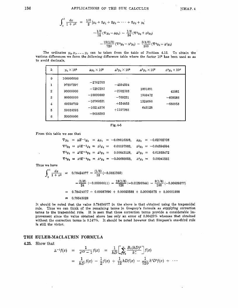
136 APPLICATIONS O F THE SUM CALCULUS [CHAP. 4
The ordinates yo, yl, . . ., can be taken from the table of Problem 4.12. To obtain the various differences we form the following difference table where the factor 10' has been used so as t o avoid decimals,
k
0
1
2
3
4
5
6
- 100000000
-2702703 97297297 -4594594
-7297297 1891891 90000000 -2702703 41581
-10000000 1933472 80000000 -769231 -609386
1324086 +554855 -680958
643128
-10769231
-10214376 69230769
59016393 $1197983 -9016393
50000000
Fig. 4-5
From this table we see that
= A E - ~ Y ~ = Ayb = -0.09016393, Ayo = -0.02702703 VY0
V2y0 = A 2 E - 2 ~ ~ = A2y4 = 0.01197983, A2yo = -0.04594594
V3y0 = A 3E-3g6 = A3y3 = 0.00643128, A3Uo = 0.01933472
V4y6 = A 4E-4y0 = A4y2 = -0.00680958, A416,-, = 0.00041581
Thus we have
- 0.78424077 - (-0.0631369) s,'& -
24 19(1'6) 720 (-0.01290344) - - 3(1'6) (-0.00639377) (1'6) (-0.03396611) - - -- 160
= 0.78424077 + 0.00087690 + 0.00023588 + 0.00005675 + 0.00001998
= 0.78543028
I t should.be noted that the value 0.78424077 in the above is that obtained using the trapezoidal rule, Thus we can think of the remaining terms in Gregory's formula as supplying correction terms to the trapezoidal rule. It is seen that these correction terms provide a considerable im- provement since the value obtained above has only an error of 0.00423% whereas that obtained without the correction terms is 0.147%. I t should be noted however that Simpson's one-third rule is still the victor.
THE EULER-MACLAURIN FORMULA

CHAP. 41 APPLICATIONS O F THE SUM CALCULUS 137
We have since A = E - 1 = ehD - 1 [see page 81
Then using property 8, page 87, with t = h D this becomes
= -f(x) 1 - 5 f ( x ) 1 + 12 1 h D f ( 2 ) - - 1 h 3 D 3 f ( ~ ) + h D 720
on using the values for Bo, B,, B,, B3, . . . .
4.26. Derive the Euler-Maclaurin formula (21) on page 124. By the fundamental theorem of sum calculus we have [see page 831
a t ( n - l l h a t n h
f(x) = A - l f b ) I (1 )
where the summation in ( I ) is to be taken from a t o a + (n - l ) h in steps of h. of Problem 4.25 we then have
Using the results
+ .. . a .t ( n - l ) h a f n h a t n h - -h3f“‘(~)
which can be written a s 1 a+nh
f(a) + f ( a + h) + * * * + f ( a + (n - 1)h ) = [ f ( 4 dx - 2 [f(a + n h ) - fb)]
I t h3 720 + 12 [ f ’ ( ~ + nh) - f’(a)] - - [f’”(a + nh) - f”’(a)] + * 9
199 1 4.27. Find 2 - by using the Euler-Maclaurin formula.
k=100
Let f(x) = l/x, a = 100, a + (n - l ) h = 199, h = 1 in the result of Problem 4.26 so that n = 100. Then f ’ ( x ) = -1/x2, f”(z) = 2%-3, f”’(x) = -62-4 so tha t
6 -&[-m+&] + * ’ *
= In2 + i (0 .005) + &(0.000075) + = 0.693147 + 0.002500 + 0.00000625 + = 0.695653
to 6 decimal places. In Problem 4.32 we shall discover how accurate the result is.
ERROR TERM IN THE EULER-MACLAURIN SERIES 4.28. Let +l,(x) = B,(x) - Bp, p = 0,1,2,3, . . ., where B p ( z ) are the Bernoulli polynomials
and Bp are the Bernoulli numbers. Show that
(4 9 ; w = ?q-m ( c ) 9,(0) = 0

138 APPLICATIONS OF THE SUM CALCULUS [CHAP. 4
(a ) We have using property 3, page 87, 3
+ b ( 4 = BL(4 = PB,-l(%) ( b ) We have since +,t l(x) =B,+l(x)-Bp+l
+:,+A4 = B;+l(x) = (P + W,(4 = (P + 1)[$fJp(4 + Bp] c:, + 1(x)
c p ( 4 = - - BP P + 1
+,(O) = Bp(0) - B, = 0 +1(x) = B,(x) - B, = x - * - (-*) = z
Then
( c ) Since by definition BJO) = B, we have
(d) We have
Thus +1(1) = 1 If p > 1 then by property 4, page 87,
+,(l) = B,(1) - B, = 0
1 p = l 0 p > 1
Then from (1) and (2) we see that
$ f J p ( l ) =
4.29. Show that
Letting x = a + hu, using the fact that +z(u) = u2 - u, and integrating by parts we have
f(x) d x = h i1 f ( a + hu) du
= $il f(a + hu) d(2u - 1) 1 1
= ; [(Zu - l ) f ( a + hu) l o - h J (2u - l ) f ’ (a+ hu) du ]
1 h = - [ f ( a ) + f ( a + h)] - 2 (2u - l ) f ’ (a + hu) du 0
= h [ f ( a ) + f ( a + h)] - 7 J1 f ’ (a + hu) d+,(u) 2 0
4.30. Show that
[?(a + h) - f’(a)l Bzh2 2 ! (a) $ J1 +z(u)f”(a + hu) du = --
+ $ +,(u)f(IV)(a + hu) du
( b ) 1’ +,(u)f(IV)(a + hu) du = -T B4h4 [?”(a + h) - f”’(a)]
+ h‘ l1 +6(U)f‘v”(a + hu) du 6! (a) From Problem 4.28(b) with p = 2 we have
qjZ(u) = -B2 + &&(u) and cdu) = &kW

CHAP. 41 APPLICATIONS O F THE SUM CALCULUS
Then
139
1 - h i1 +;(u)f(v)(a + hu) du
B4h4 - -- [f”’(u + h) - f”’(a)] - - ;y i1 +5(u)f(v)(a + hzc) du - 41
B4h4 he - - -- [f”’(a+ h) - f”’(a)] - zs &(u)f‘v’(a+ hu) du 0 4!
4.31. Obtain the Euler-Maclaurin series with a remainder for the case where n = 1 [see equation (a+$), page 1251.
From Problems 4.29 and 4.30 we have
+ 5 I’ +8(u)f‘””(a + hzt) du
which is the required result. This result can of course be generalized and leads to that on page 125.

140 APPLICATIONS O F T H E SUM CALCULUS [CHAP. 4
4.32. Estimate the error made in the approximation to the sum in Problem 4.27. Using f(x) = 1/x, a = 100, h = 1, n = 100, rn = 3 in the result of Problem 4.27 we can
write i t as
6 1 - R
where
] d u
Now by the mean-value theorem for integrals we have
Thus the absolute value of the error i s . 99
But since O < 5 < 1, i t follows tha t each term in the series on the right is less than l / ( l O O ) 7 and so the sum of the first 100 terms of the series is less than l O O / ( l O O ) 7 so tha t
The fact tha t the error i s so small shows tha t not only is the result 0.695653 accurate to 6 decimal places but t h a t we could have obtained accuracy to 12 decimal places at least by simply obtaining more decimal places i n Problem 4.27. If we do this we find
199
2 k=100
- = 0.693147180559945 + 0.0025 + 0.00000625 + 0.000000000078125
= 0.695653430638
accurate to all 12 decimal places.
more decimal place accuracy [see Problem 4.751.
since one then can determine how many figures in a calculation a re accurate.
By taking only one more term in the Euler-Maclaurin formula i t is possible to obtain even
This problem serves to illustrate fur ther the importance of being able to find a n error term
STIRLING'S FORMULA FOR n ! 4.33. Prove that
1 1
Inn! c + ( n + i ) ~ n n - n + - - I +
12n 36Qn2 * . .
where c is a constant independent of n.
Let f(x) = l n x , h = 1 in the Euler-Maclaurin formula. Then
Y
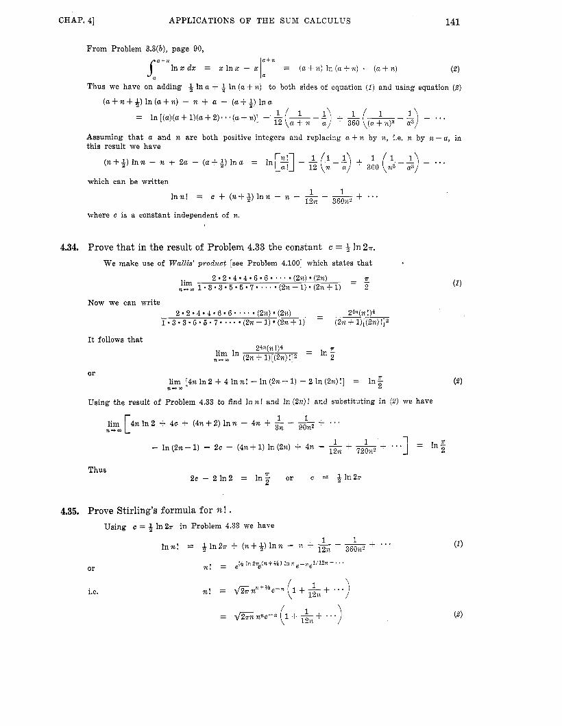
CHAP. 41 APPLICATIONS O F THE SUM CALCULUS 141
From Problem 3.3(b), page 90,
(2) l n x d x = x l n x - x = ( a + n ) In ( a + n ) - ( a + n ) latn Thus we have on adding 8 In a + In ( a + n) to both sides of equation ( I ) and using equation ( 2 )
Assuming that a and n are both positive integers and replacing a + n by n, i.e. n by n - a, in this result we have
which can be written 1 1 Inn! = c + ( n + + ) l n n - n + - - + 12n
where c is a constant independent of n.
4.34. Prove that in the result of Problem 4.33 the constant c = & ln2r. We make use of Wallis' product [see Problem 4.1001 which states that
n - - - 2 2 4 4 6 6 * * - (2n) (2%) (2% - 1) ' (2% + 1) lim
12'- 1 . 3 - 3 . 5 . 5 . 7 . * 2
Now we can write 2 2 - 4 4 9 6 6 - . * - (2n ) (2%)
1 . 3 . 3 . 5 . 5 . 7 . .... (2n - 1) (2% + 1) - 2 9 n !)4
- (2% + 1 ) [ ( 2 n ) ! ] z
It follows that
or lim [4n In2 + 4 Inn ! - In ( 2 n + 1) - 2 In ( 2 n ) ! ] = In' 2
n-+m
Using the result of Problem 4.33 to find In n! and In (2%) ! and substituting in (2) we have
or
i.e.
4.35. Prove Stirling's formula fo r n ! . Using c = 4 In 2a in Problem 4.33 we have
1 1 Inn ! = q l n 2 n + (n++) Inn - n + 12n - +
! = e% In2rre(n t M ) In n e-ne1/12n -, '
n!
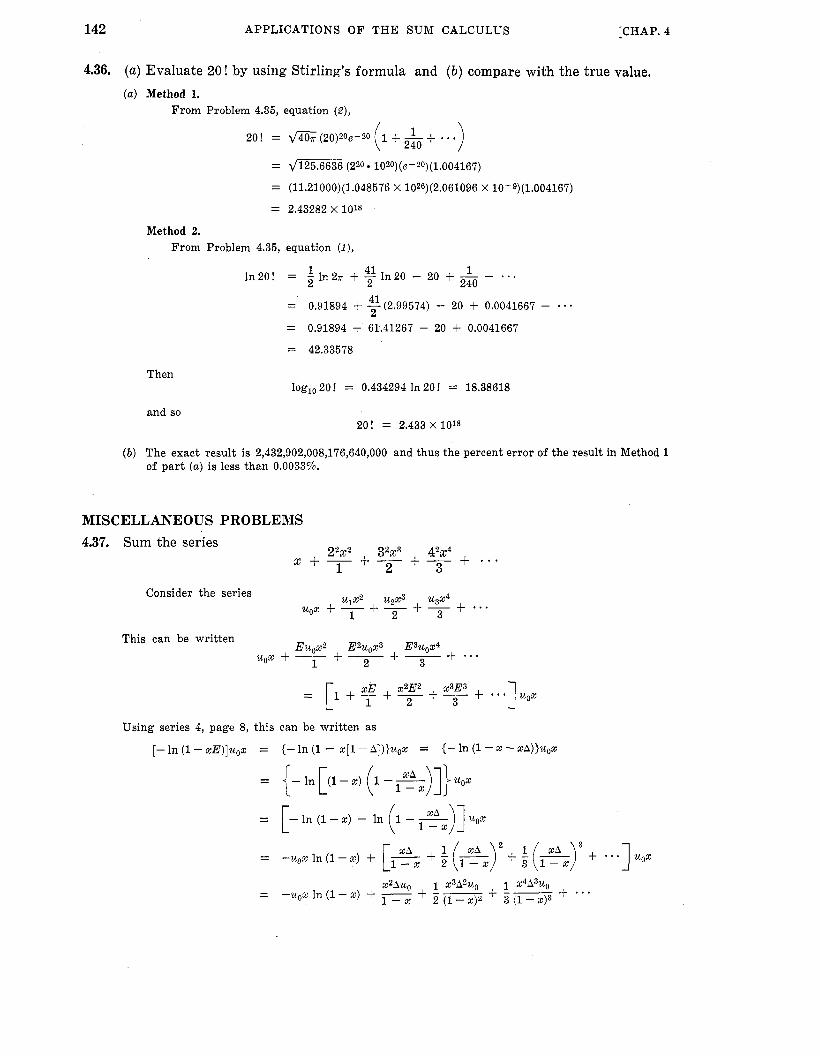
142 APPLICATIONS O F T H E SUM CALCULUS [CHAP. 4
4.36. (a) Evaluate 20! by using Stirling's formula and ( b ) compare with the true value. (a) Method 1.
From Problem 4.35, equation (2 ) ,
20! =
- -
- - - -
Method 2. From Problem 4.35,
ln20!
Then
and so
q-6 (220 1020)(~-zo)(1.004167)
(11.21000)(1.048576 X 1026)(2.061096 X 10⁻⁹)(1.004167)
2.43282 X 10¹⁸
equation ( I ) ,
1 41 1 2 2 240 = - In27 + - In20 - 20 + - - * .
= 0.91894 + -(2.99574) 41 - 20 + 0.0041667 - * . * 2
= 0.91894 + 61.41267 - 20 + 0.0041667
= 42.33578
log,, 20! = 0.434294 In 20! = 18.38618
20! = 2.433 X 10'8
( b ) The exact result is 2,432,902,008,176,640,000 and thus the percent error of the result in Method 1 of par t (a) is less than 0.0033%.
MISCELLANEOUS PROBLEMS 4.37. Sum the series
+ . . . 22x2 32x3 42x4
2 $3 + - x + - 1
Consider the series u1x2 u2x3 u3x4 uox + ~ + - + - + . * . 1 2 3
E U ~ X ~ E~uOX~ E~uOX~ 1 2 3
This can be written uox + - + - + - + * . *
= [Ili+-+-+... x E x2E2 x3E3 2 3
Using series 4, page 8, this can be written as
[-In (1 - xE)]uox = {-In (1 - x [ l f A])}uox = {-In (1 - x - xA)}uox
x ~ A u O 1 X ~ A ~ U O 1 x4A3Uo + ... 1 - x + 5(1--.)2 + 2- = -u0x In (1- x) + -

CHAP. 41 APPLICATIONS OF THE SUM CALCULUS
u, Au, Azu, A ~ u ,
3
5
7
9
n = O 1
2 n = l 4
n = 2 9 2
2 n = 3 16
n = 4 25
0
0
c
143
~~
Fig. 4-6
Thus u, = 1, Au, = 3, A%, = 2, A3u0 = 0, A4u0 = 0, .
Then the sum of the series is 3x2 - 2x3 - - x ln(1-x) -x In (1 - x) + - +- 3x2 23 -
1 - x ( 1 - X ) Z (1 - x p
4.38. Prove Weddle’s rule [equation (16), page 1231.
In doing this we need the terms involving A5f(a) and Aef(a) which are not given in Problem 4.9 but are presented in Problem 4.60.
Put n = 6 in Problem 4.9 and neglect differences of order 6 and higher.
We then find
9
41 11 41 + ~0 A4f(a) + %A5f(a) + 840 A6f(a)]
[ a + 6 h
.(: f(x) dx = 6h f ( a ) + 3Af(a) + 2A2f(a) + 4A3f(a)
6f(a) + 18Af(a) + 27Azf(a) + 24A3f(a)
Now if we change the coefficient 41/140 to 42/140 = 3/10 the error made is quite small. make this change we obtain the approximation
If we
r a t e h f ( ~ ) d r = h r 6 f ( a ) + 18Af(a) + 27AZf(a) + 24~3f(a) L
= [ { f ( a ) + f ( a + 2h) + f(a + 4h) + f ( a + 6h))
+ 5{f(a + h) + f ( a + 5h)3 + 6f(a f 3h)]
The result can be extended to evaluate f(x) dx when N is a multiple of 6 [see Problem 4.911.
4.39. (a) Work Problem 4.12 by Weddle’s rule and ( b ) compare the result with the exact value and that obtained by Simpson’s one-third rule and Simpson’s three-eighths rule.
(a) We can use the table of Problem 4.12 since N = 6. Then using Problem 4.38 we have
3O [(l .OOOOOOOO + 0.90000000 + 0.69230769 + 0.50000000) So1& = 10 + 5(0.97297297 + 0.59016393) + 6(0.80000000)]
= 0.78539961

144 APPLICATIONS O F T H E SUM CALCULUS [CHAP. 4
Rule
Trapezoidal Simpson's one-third Simpson's three-eighths Weddle's
Percent error
0.147% 0.00028% 0.00293% 0.00185%
Supplementary Problems SERIES OF CONSTANTS 4.40. Sum each of the following series to n terms by using the method of Problem 4.1, page 126.
(a) 1 + 3 + 5 + 7 + * ' . (e) 1 3 + 23 + 33 + 43 + (b) 1 2 + 32 + 52 + 72 + . * . (f) 1 . 3 . 5 + 3 0 5 . 7 + 5 . 7 . 9 + (c) 22 + 52 + 82 + 112 + * * (9) 1 . 2 9 5 + 2 . 3 0 6 + 3 . 4 - 7 + (d ) 2 . 4 + 4 . 6 + 6 . 8 + * * . (h) 3 . 5 0 1 0 + 4 . 6 0 1 2 + 5 - 7 - 1 4 + * a *
4.41. Sum the series l2 + 22% + 32x2 + 42x3 + * * . 4.42. Can the series of Problem 4.41 be summed to n terms? Explain.
22 32 42 52 62 3 32 33 34 35 4.43. Sum the series 1 2 - - + - - - + - - - + * * . .
POWER SERIES 4.44. Sum the series
(a) x + 2x2 + 3x3 + 4x4 + a ' '
(b) 3 2 + 22x2 + 32x3 + 42x4 + (c) 193 + 3.623 + 5'7x2 + 709x3 + * * -
' ' *
2 . 5 5 . 8 8.11 11.14 I . . . 36 38 4.45. Sum the series - - - 32 34
1 2 32 52 72 4.46. Sum the series 5 + + 3 + a + * .
4.47. I f
and
show t h a t
= A(%) s i n x + B(x ) cosx

CHAP. 41 APPLICATIONS O F T H E SUM CALCULUS 145
33x3 5325 73x7 2 ! 4! 6!
4.48. Sum the series 13x - - + - + - + * . 4.49. Sum the series
12x 22x2 32x3 ~ 42x4 I . . . - + - + - l! 3! 5! 7 !
4.50. Can the power series method of page 121 be used for the finite series
22x2 32x3 42x4 n2xn + - 1 3 + __ + - + - + ... 3 32 33 34 3n
4.51. Can the sum of the first n terms of the series of Problem 4.48 be found by using the power series method of page 121? Explain.
APPROXIMATE INTEGRATION
4.52.
4.53.
4.54.
4.55.
4.56.
4.57.
4.58.
4.59.
4.60.
Find x 3 $ by using the extended trapezoidal rule where the interval of integration i s subdivided
into (a) 6 (b) 10 equal parts. Show tha t the t rue value is I n 3 = 1.09861 approx. and compare this with the values obtained in (a) and ( b ) .
Discuss how you would improve the accuracy in Problem 4.52,
Work Problem 4.52 by using Simpson’s one-third rule and discuss the accuracy.
Show tha t Simpson’s one-third rule is exact if f (x) is a polynomial of degree 3. metrical significance of this?
(a) Work Problem 4.52(a) by using Simpson’s three-eighths rule and discuss the accuracy. you work Problem 4.52(b) by Simpson’s rule?
Derive the extended Simpson’s three-eighths rule.
What is a geo-
( b ) Can Explain.
Explain the difficulty involved in attempting to find the approximate value of
without actually evaluating the integral.
Can you resolve the difficulty i n par t (a)?
Prove the formula
where yk = f ( a + kh).
Use (a) to obtain an approximate value for
and compare with the exact value.
Show t h a t the next two terms in the series for
{ a i n h f ( 2 ) dx
given in equation (8), page 122, a r e n(Zn4 - 24x3 + 105n2 - 200% + 144)
1440 A 5 f ( a )
n(12ns - 210124 + 1 4 2 8 ~ 3 - 4725n2 + 7672n - 5040) Asf (a ) 60,480 +
and use this to complete the proof in Problem 4.38.

146 APPLICATIONS O F T H E SUM CALCULUS
X
f(x)
[CHAP. 4
0 0.2 0.4 0.6 0.8 1.0
1.00000 0.81873 0.67032 0.54881 0.44933 0.36788
T / 2 4.61. Find a n approximate value of sin x dx and compare with the exact value.
4.63. Discuss what steps you would use to work Problem 4.62 if the values corresponding to (a) x = 0.4 (b ) x = 0.4 and x = 0.8 were not present in the table.
THE EULER-MACLAURIN FORMULA 4.64. Use the Euler-Maclaurin formula to find the sums of the series
(a) 1 2 + 22 + 32 + . * ' + n 2
(c) 1 ' 2 + 2 . 3 + 3 . 4 + . " + n ( n f 1 )
(d ) 1 4 + 24 + 34 +
(b) 1 3 + 23 + 33 + . . - $- n3
4.65. Use the Euler-Maclaurin formula to work Problem 3.46, page 108.
1 1 1 1 1 1 1 - + - + 3 t ... + - 1 2 n 2n 12n2 Eon4 4.66. Show tha t = y + I n n + - - - f - -
where y is Euler's constant.
4.67. Use Problem 4.66 to obtain an approximate value for y.
4.69. Show t h a t
to 5 decimal place accuracy by using the Euler-Maclaurin 1 1 1 4.70. Sum the series - + - i - + * 1 3 23 33 formula.
ERROR TERM IN THE EULER-M$CLAURIN FORMULA 4.71. Show tha t
4.72. Obtain the Euler-Maclaurin formula with a remainder for the case where m = 5 .

147 CHAP. 41 APPLICATIONS O F THE SUM CALCULUS
4.73. (a) Use mathematical induction to extend the results of Problems 4.71 and 4.72 and thus ( b ) prove result (23), page 125.
4.74. Prove the result (25) , page 125.
4.75. (a) Show how to improve the accuracy of the result in Problem 4.32 by taking one more term in the Euler-Maclaurin formula. ( b ) Determine the accuracy of the result obtained in par t (a) .
4.76. Prove t h a t if f(*P-”(x) does not change sign in the interval from a to a, + nh then the remainder R given in the Euler-Maclaurin formula ( 2 4 ) , page 125, has the property t h a t
4.77. Work ProbIem 4.70 by taking into account the error term in the Euler-Maclaurin formula.
STIRLING’S FORMULA FOR n! 4.78. Obtain lo! f rom Stirling’s formula and compare with the exact value.
(?;) * 4.79. Calculate the approximate value of the binomial coefficient
4.80.. Use Stirling’s formula to show tha t 2?n(n ! ) 2 fi = lim ~
n+o (2?z)! f i and show tha t the result i s equivalent t o Wallis’ product.
1 4.81. Show t h a t for large values of n (-Y2) =
4.82. Generalize the result of Problem 4.35 to obtain
n ! = *nne-n
MISCELLANEOUS PROBLEMS (12 + l )x (22 + 2)x2 + (32 + 3)23 - . . .
4.83. Sum the series ~ - l! 2 ! 3 !
1 1 1 4.84. Sum the series 1.3.7 + 3.5.9 + m1 + * 3 * (a) to ?z terms and ( b ) to infinity.
4.85. Show t h a t (x- 1 ) 2 + * “ + (x - 1 ) n n(n - 1) (n - 2)
3! ( x - 1 ) + n(n - 1) 1 + x + x 2 + - - * + x n = n + T
4.86. Find a n approximate value f o r L ’ & .
4.87. Obtain a n approximate value for the integral
t T ” x cot x dx
and compare with the exact value given by -6. In 2 = -1.0888. . , .
4.88. (a) Use integration by par t s and the result of Problem 4.87 to find T I 2
In s ine de
( b ) Explain why numerical methods a re not immediately applicable to the integral in (a).

148 APPLICATIONS O F THE SUM CALCULUS [CHAP. 4
4.89.
4.90.
4.91.
4.92.
4.93.
4.94.
4.95.
4.96.
4.97.
Obtain equation ( 5 ) of Problem 4.19 and thus complete the proof in tha t problem.
Show t h a t the seventh differences in Weddle's rule drop out and explain the significance of this.
Derive Weddle's extended rule.
Show t h a t
These a re sometimes called Euler transformations and are often useful for speeding up the con- vergence of slowly convergent series.
Show how Problem 4.92 can be used to find a n approximate value fo r the series
1 1 1 1 1 - - - + - - - + - - .. 1 3 5 7 9 ( b )
and compare with the exact values given by In 2 and 714 respectively.
Sum the series 1 2 - 22 + 32 - 4 2 + - 9 . + (-1)n-1n2.
Sum the series 1 2 + 2 22 + 4 32 + 8 42 + 16 52 + - - to n terms.
If x # -1, -2, -3, . . . show t h a t
1 + ... = - 1 l! 2! x+l + F+ l ) ( x + 2 ) + (x+ l ) ( x + 2 ) ( x + 3 ) X
+- + R 1 1 1 ~ + ~ +, ... = - (n + 1 ) 2 (n + 2)2 n + 1 2(n+ 1 ) 2
Show t h a t
O S R S A 6(n + l ) 3 where
4.98. Let f(x) have the values yo,y1,y2 at x = a, a + h, a + 2h respectively.
(a) Obtain an interpolating polynomial f o r f ( x ) .
( b ) Use the interpolating polynomial i n (a) to obtain the approximate result
h - [ 5 f ( a ) + 8 f ( a + h) - f ( a + 2h)] a + h
f(x) dx = s, 12
( c ) Use the interpolating polynomial in (a) to obtain the approximate result 1"" f ( x ) dx = [2f(a + h) - f ( a + 2h) + 2f(a + 3h)]
(d) Show tha t the formula in ( c ) is exact when f(x) is a polynomial of degree 3 but that the formula in ( b ) is not exact in such case.
4.99. Use the results of Problem 4.98(b) and ( c ) to obtain approximate values of
and discuss the accuracy.
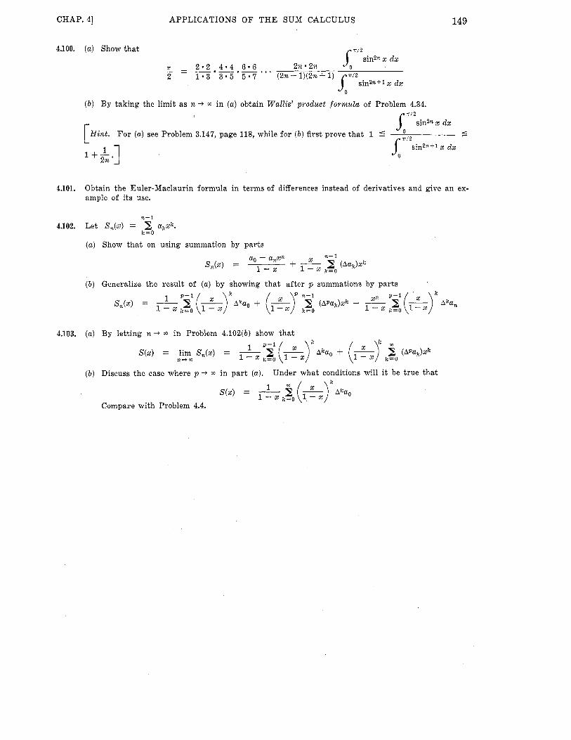
CHAP. 41
4.100. ( a ) Show tha t
APPLICATIONS O F T H E SUM CALCULUS 149
( b ) By taking the limit as n + m in (a) obtain Wallis' product formula of Problem 4.34. T / 2 1 sinznx dx
Hint. For (a) see Problem 3.147, page 118, while for ( b ) first prove tha t 1 S 7,2
d sin2nfl x dx
1+&] 2n
[
4.101. Obtain the Euler-Maclaurin formnla in terms of differences instead of derivatives and give an ex- ample of its use.
n- 1
k=O 4.102. Let S,(s) = 2 akxk.
(a) Show t h a t on using summation by par ts
( b ) Generalize the result of ( a ) by showing tha t af ter p summations by par ts
4.103. ( a ) By letting n + m in Problem 4.102(b) show t h a t
( b ) Discuss the case where p --3 m in par t (a ) . Under what conditions will i t be t rue that k
S ( x ) = - l - x k = O 1 5 (-) 1--x Aka,
Compare with Problem 4.4.

DIFFERENTIAL EQUATIONS In previous chapters we have examined the remarkable analogies which exist between
the difference and sum calculus and the differential and integral calculus respectively. I t should thus come as no surprise that corresponding to the theory of differential equations there is a theory of difference equations.
To develop this analogy we recall that a differential equation is a relationship of the form
between x and the derivatives of an unknown function y = f ( x ) . dnyldxn in (1) we obtain
If we can solve for
and we call the order n of this highest derivative the order of the dif ferential equation.
A solution of a differential equation is any function which satisfies the equation, i.e., re- duces i t to an identity when substituted into the equation. A general solution is one which involves exactly n arbitrary independent constants. A particular solution is a solution obtained from the general solution by assigning particular values to these constants.
Example 1. The equation - 3 * + 2y = 4x2 is a differential equation of order two. A general solution is
dx2 dx y = cle5 4- c2e2S + 2x2 + 6x + 7 [see Problem 5.11 and a particular solution is y = 2eZ - 6e2Z f 2s2 + 60 4- 7.
To determine the n arbitrary constants we often prescribe n independent conditions called boundary conditions for the function y . The problem of determining solutions of the differential equation subject to these boundary conditions is called a boundary-value prob- l em involving differential equations. In many cases differential equations arise from mathematical o r physical problems and the boundary conditions arise naturally in the formulation of such problems.
DEFINITION OF A DIFFERENCE EQUATION
tionship of the form By analogy with differential equations we shall define a difference equation as a rela-
(3)
150

CHAP. 51 DIFFERENCE EQUATIONS 151
Since Ax = h [and since by custom or convention (Ax)” = hP is written Axp when appear- ing in the denominator] we see that the difference equation ( 3 ) is a relationship connecting x, y, a y , a2y, . . . , any or equivalently x, f(x), f(x + h), f (x + 2h), . . . , f(x + nh) since y = f(x). Thus we can define a difference equation as a relationship of the form
G(x, f(x), f(x + h), f(x + 2h), . . . f(x + nh)) = 0 (4 where f(x) = y is the unknown function.
ORDER OF A DIFFERENCE EQUATION From the analogy with differential equations it might be suspected that we would
define the order of a difference equation as the order of the highest difference present, i.e. n in (3) or (4). However this leads to some difficulties [see Problem 5.51 and so instead we define the order to be the difference between the largest and smallest arguments for the function f involved divided by h. Thus in (4) if both f(x) and f ( x + nh) appear explicitly the order is [(x + nh) - x ] / h = n. However if f(x) does not appear but f ( x + h) and f(x + nh) both appear then the order is [(x + nh) - (x + h)]/h = n - 1.
SOLUTION, GENERAL SOLUTION AND PARTICULAR SOLUTION OF A DIFFERENCE EQUATION
A solution of a difference equation is [as in the case of differential equations] any function which satisfies the equation. A general solution of a difference equation of order n is a solution which involves n arbitrary periodic constants [as on page 821. A particular solution is a solution obtained from the- general solution by’ constants.
Example 2. The equation *- 3 @ + 2y = 4 ~ ( ~ ) , which can be written as Ax2 Ax
f(x + 2h) - (3h + 2)f(x + h) + (2h2 + 3h + l)f(X)
where y = f(x), is a difference equation of order 2. A general solution
y = f(x) = Cl(X)(l+ 2h)X/h + as can be verified by substitution [see Problem 5.41.
cl(x) = 2 + 4h sin ( 2 ~ x l h ) ,
both of which have periods h.
To determine the n arbitrary periodic we can prescribe n independent boundary
assigning par-ticular periodic
= 4h2,tz)
is given by
c2(x)(l + h ) x / h + 2x2 + (6 - 2h)x + 7
A particular solution is found for example by letting
cz(x) = 5 + h2[1 - cos (28Xlh)I
constants of an nth order difference equation conditions for the unknown function y . The
problem -of determining solutions to the difference equation subject to these boundary con- ditions is called a boundary-value problem involving difference equations. As in the case of differential equations these may arise from the nature of a mathematical or physical problem.
DIFFERENTIAL EQUATIONS AS LIMITS OF DIFFERENCE EQUATIONS I t will be noted that the limit of the difference equation of Example 2 as Ax = h ap-
proaches zero is the differential equation of Example 1. Also the limit of the solution of the difference equation as a x = h approaches zero is the solution of the differential equation [see Problems 5.6 and 5.71.

152 DIFFERENCE EQUATIONS [CHAP. 6
In general we can express a differential equation as the limit of some corresponding difference equation.
USE OF THE SUBSCRIPT NOTATION
f ( a + kh) can be written as
If we are given the n values zjo,y~,y~, . . . , yn -1 then we can determine yk for k=n,n+l,. . . . Example 3.
If the subscript notation is used, the difference equation (4 ) with x = a + kh, gk =
H ( k , y k , y k + l , . . ., y k f n ) = 0 (5)
The difference equation f ( x + 3h) - 6f(x + 2h) + 6f(x + h) + 3 f ( ~ ) = 0
can be written in subscript notation a s
Y k t 3 - b k + 2 + 6 ~ k + 1 + 3 Y k = 0 Then given yo = 1, y, = -2, y2 = 0 we find on putting k = O,l, , . . the values y3 = 9, y4 = 61, . . . .
The difference equation (5 ) can also be written in terms of the operator E, i.e.
H ( k , y k , E y k , E 2 y k , . . . , E n y k ) = 0 (6) Example 4.
The difference equation of Example 3 can be written a s
( E ' - 6 E 2 + 6 E + 3 ) ~ k = 0
LINEAR DIFFERENCE EQUATIONS An important class of difference equations which arises in practice is a linear differ-
ence equation. A linear dif ference equation of order n is a difference equation having the form ao(k)E"yk + a l ( k ) E " - l y k f ' * ' + an(k)yk = R(k) (7)
where ao(k) # 0. This equation can also be written as
[ao(k)E" + al(k)En-' + - * + an(k)]yk = R ( k )
where the linear operator +(E) is given by
+(E) = ao(k)E" + al (k)En- l + * * * + an(k)
A particularly important case arises when ao(k), a ~ ( k ) , . . . , an(k) are all constants [i.e. independent of k ] and in such case we refer to (7) , (8) or (9) as a linear dif ference equation of order n with constant coefficients.
A difference equation which does not have the form (7) , (8) or (9), i.e. which is not linear, is called a nonlinear d i ference equation. Example 5.
The equation of Example 4 is a linear difference equation with constant coefficients.
Example 6.
variable] coefficients.
Example 7.
The equation [(2k + 1)E2 - 3kE 4- 4 ] y k = 4 k 2 - 3k is a linear difference equation with nonconstant [i.e.
The equation Y k y k + l = yE-l is a nonlinear difference equation.

CHAP. 51 DIFFERENCE EQUATIONS 153
HOMOGENEOUS LINEAR DIFFERENCE EQUATIONS If the right side of (8) is replaced by zero we obtain
(uOE" + aiEn-l + * * + an)yk = 0 (11) or $(E)gk = 0 (12) which is called the homogeneous equation corresponding to (9 ) . It is also called the reduced equat ion and equation ( 9 ) is called the complete equation or nonhomogeneous equation. Example 8.
The difference equation of Example 4 is a homogeneous linear equation.
Example 9. The homogeneous equation corresponding to the complete equation of Example 6 is
It turns out that in order for us to be able to solve the complete equation (9) we first need to solve the homogeneous or reduced equation (12) [see Theorem 5-3 below].
Since the general theory of linear difference equations is in many ways similar to that of linear difference equations with constant coefficients we shall consider this simplified case first.
[ (2k + 1)E' - 3kE + 4]yk = 0
HOMOGENEOUS LINEAR DIFFERENCE EQUATIONS WITH CONSTANT COEFFICIENTS
stants. Then on substitution we obtain Assume that y k = rk is a solution of (11) where we suppose that U O , al, . . . , an are con-
U O P + ~ + a l ~ n + k - l + . - - + anrk = 0 or (norn + a1P-l + * * * + an)? zz 0 It follows that rk is a solution of (9) if T is a solution of
aorn + alTn-1 + * * ' + a, = 0
which is called the auxi l iary equat ion and can be written +(r) = 0. roots which we take to be TI, r2, . . . , rn which may or may not be different. (11) can be written in f ac tored form as
(13) This equation has n
In such case
aO(E-?"l)(E-r2). ' . . ( E - T n ) p k - 0 - (1-4) Solutions of (14) depend on the nature of the roots rl, . . . , r,. The following cases can
arise. Case 1. Roots are all real and distinct.
Since constant multiples of these solutions are also solutions and since sums of solutions are solutions [because +(E) is a linear operator] we have the solution
y k = clrt + c2r,k + Case 2. Some of the roots are complex numbers.
If ao, al, . . . , an are assumed to be real it follows that complex roots if they occur must be conjugate complex numbers, i.e. if ,+pi is a root then so also is ,-pi where a and p are real. In this case
In this case r : , ~ : , . . .,rk are all solutions of (11).
* + cnrk
and (.-pi)" are solutions and so we have the solution Kl((Y + p i ) k + K2(a - p i ) k
where K1, K2 are constants. To get this in real form we write the complex numbers in polar form, i.e.
(Y + pi = p(cos 6 + i sin e), (Y - pi = p(cos 6 - i sin 6)

156 DIFFERENCE EQUATIONS [CHAP. 5
The only requirement which must be met to guarantee success of the method is that no term of the trial solution can appear in the complementary function. If any term of the trial solution does happen to be in the complementary function then the entire trial solution corresponding to this term must be multiplied by a positive integer power of k which is just large enough so that no term of the new trial solution will appear in the complementary function. The process is illustrated in Problems 5.20-5.22.
SPECIAL OPERATOR METHODS We have seen that any linear difference equation can be written as
#(E)% = R(k) (18)
---R(k) = U where +(E)U = R(k ) (19) $(E)
Let us define the operator 1/@) called the inverse of +(E) by the relationship 1
We shall assume that U does not have any arbitrary constants and so is the particular solution of the equation (18). We can show that l/+(E) is a linear operator [see Problem 5.241.
The introduction of such inverse operdtors leads to some special operator methods which are very useful and easy to apply in case R(k) takes on special forms as indicated in the following table. In this table P(k ) denotes as usual a polynomial of degree m. For illustrations of the methods see Problems 5.23-5.30.
1. ~ ( p ) f 0, otherwise use method 4.
1 +(E)
sinuk or -coscuk 2. - d E )
Write cosak = 9 sinak = eik + e-tk eiak - e-iak
and use 1. 2
P(k ) = ~ P ( k ) = (9, + blA + 3. - + bmAm + * * * ) P ( k ) 1 +(I+ A) +(El
where the expansion need be carried out only as f a r as Am since A m + I P ( k ) = 0.
pkP(k) = pk- P(k) . Then use method 3. 1 dPE)
The result also holds for any function F(k) in place of P(k) .
Fig. 5-2
I
METHOD OF VARIATION OF PARAMETERS In this method we first find the complementary solution of the given equation
+(E)yk = R k (20)
i.e. the general solution of +(E)’h = 0
in the form yk = C I U ~ + czuz + * * * + CnUn

DIFFERENCE EQUATIONS 157 CHAP. 61
We then replace the arbitrary constants c1, CZ, . . . , Cn by functions of k denoted by Ki, Kz, . . . , Kn and seek to determine these so that
f/k = Klul + K ~ U Z + * * ' -t Knun (28) satisfies (20). Since n conditions are needed to find K I , K z , . . ., Kn and one of these is that (20) be satisfied there remain n - 1 arbitrary conditions which can be imposed. These are Usually chosen so as to simplify as much as possible the expressions for Ayk,A2yk, , . . . The equations obtained in this way are
(24) 1 ul& + u 2 ~ K 2 + . - . + UnAKn = 0 (AUn)AKn = O ( A U ~ ) A K , + ( A U ~ ) A K ~ + * * * +
. . . . . . . . . . . . . . . . . . . . . . . . . . . . . . . . . . . . . . . . . . . . . . (An-'Ul)AK1 + ( A ~ - ~ u ~ ) A K ~ + *
(hn-lul)aK1 + (An-%2)AKz * + (An-'Un)AKn = O
* * * + (An-lUn)AKn = R k
which can be solved for aK1 ,aKz , . . ., AKn and thus K1, Kz, . . ., Kn from which (23) can be found. For an illustration of the method see Problem 5.31. It should be noted that the determinant of the coefficients of (2.4) is equal to the Casorati of the system [see (15)] which is different from zero if ~1,242, . . . , U n of (23) are linearly independent. See Problem 5.104.
METHOD OF REDUCTION OF ORDER If an nth order equation can be written as
(E - Tl)(E - r z ) * * * (E - Tn)f/k = R k (25)
( E - T i ) Z k = R k (26)
then on letting zk = ( E - r2) * - ( E - rn)yk we are led to the first order equation
which has the solution k-l RP
z k = ($) = T: rptl -/- Clr: P = l 1
where CI is an arbitrary constant. By continuing in this manner (25) can be solved.
METHOD OF GENERATING FUNCTIONS The generating func t ion fo r yk is defined as
G ( t ) = 5 yktk k = O
By using this a linear difference equation can be solved. See Problem 5.34.
LINEAR DIFFERENCE EQUATIONS WITH VARIABLE COEFFICIENTS
using the fundamental Theorem 5-3, page 155. difference equations with variable coefficients it can also be used to solve such equations.
Up to now we have considered linear difference equations with constant coefficients by Since this theorem also applies to linear
Any linear first order equation with variable coefficients can be written as
y k f i - Akyk = R k or ( E - A k ) Y k = R k (29)
and can always be solved. The solution is given by

158 DIFFERENCE EQUATIONS [CHAP. 5
where c is an arbitrary constant. This solution can be obtained by multiplying both sides of (29) by the summation factor uk = 1 / A l A 2 . ' A k - 1 analogous to the integrating factor fo r first order differential equations. See Problem 5.35.
Second or higher order linear equations with variable coefficients cannot always be solved exactly. In such cases special methods are used. Among the most common methods are the following.
1.
2.
3.
4.
Factorization of the operator. In this method we attempt to write the difference equa- tion as
(31)
by finding A k , B k , . . ., u k and then using the method of reduction of order. lems 5.36 and 5.37.
Variation of parameters. This can be used when the complementary solution can be found. See Problem 5.114.
Generating functions. See Problem 5.124.
Series solutions.
See Prob-
In this method we assume a solution in the form of a factorial series
(32)
where c, = 0 for p < 0. See Problem 5.38.
STURM-LIOUVILLE DIFFERENCE EQUATIONS A Sturm-Liouville difference equation is one which has the form
A ( P k - d y k - 1 ) f ( q k + h r k ) y k = 0 where 1 5 k 5 N - 1 and where h is independent of k .
(33)
We shall associate with (33) the boundary conditions
a,Y, + a1Y1 = 0, ayNY, + @ N + I Y N + l = 0 (34) where a,, al, aN, aNtl are given constants.
We seek nontrivial solutions [i.e. solutions which are not identically zero] of the equation (33) subject to conditions (34). The problem o f finding such solutions is called a Sturm- Liouville boundary-value problem. The equations (33) and conditions (3.4) are called a Sturm-Liouville szjstem.
We can show that in general there will be nontrivial solutions only for certain values of the parameter h. The solutions corresponding to these are then called characteristic functions or eigenfunctions. In general there will be a discrete set of eigenvalues and eigenfunctions. If Am and An are two different eigenvalues we can denote the corresponding eigenfunctions by +7n, and +n,k respectively.
In case p k , q k , rk are real we can show that the eigenvalues are also real [see Prob- lem 5.401.
These values are called characteristic values or eigenvalues.
If the eigenfunctions are real we can also show that N c r k + m , k + n , k = ' if (35)
k = l

’ DIFFERENCE EQUATIONS 159 CHAP. 51
In general we can take r k > 0. Then (35) states that the eigenfunctions {fi+m,k} where m = 1, , . ., N are mutually Orthogonal. The terminology used is an extension to N di- mensions of the idea of orthogonality in 3 dimensions where two vectors A = A l i + A 2 j + A&, B = Bli + B 2 j f B& are orthogonal or perpendicular if
3
(36) AIBI f AZBZ + AJ33 = 0 i.e. 2 AkBk = 0 k = l
The extension to N dimensions is obtained on replacing the upper limit 3 in the sum by N thus yielding (35) .
In case (35) holds we also say that the functions {+m,k} are orthogonal with respect to the weight or density r k .
Given a function Fk it is often possible to obtain an expansion in a series of eigenfunc- tions. We find that
N
Fk = C cm+m,k (37) m = l
where the coefficients cm are given by N
k = l 2 rkFk+m,k
2 ‘k+h, k k=l
Cm = N m = l , ..., N
If we suitably normalize the functions +m,k so that N
then the coefficients (38) are simplified since the denominator is equal to 1. (35) and (39) can be restated as
The results
N 0 m P n k=i 1 m = n
In such case we say that the set {fi+m,k} is an orthonormal set.
NONLINEAR DIFFERENCE EQUATIONS ’
transformations which change them into linear difference equations. and 5.44.
An important class of nonlinear difference equations can be solved by applying suitable See Problems 5.43
SIMULTANEOUS DIFFERENCE EQUATIONS If two or more difference equations are given with the same number of unknown
functions we can solve such equations simultaneously by using a procedure which elimi- nates all but one of the unknowns. See for example Problem 5.45. ~
MIXED DIFFERENCE EQUATIONS In addition to differences which may occur in equations there may also be derivatives
In such case we refer to the equations as differential-difference equations, These equations can sometimes be solved by various
or integrals. integral-difference equations, etc. special techniques. See Problems 5.46 and 5.47 for example.

160 DIFFERENCE EQUATIONS [CHAP. 5
PARTIAL DIFFERENCE EQUATIONS Up to now we have been concerned with difference equations involving unknown func-
tions of one variable. These are often called ordinary dif ference equations in contrast to difference equations involving unknown functions of two or more variables which are called partial difference equations.
To consider such equations we must generalize the concepts of difference operators to functions of two or more variables. To do this we can consider for example a function f ( x , y) and introduce two difference operators AI, AZ defined so that if h = Ax, 1 = Ay are given,
A f ( x , 9) = f ( x + h, y) - f ( x , Y), Azf (X, y ) = f ( x , Y + 1) - f ( x , V ) (41)
These are called partial difference operators. Similarly we define partial translation oper- ators El, Ez so that
Elf(%, Y) = f ( x + h, Y ) , Ezf(x, Y ) = f ( x , Y + 1) (42)
El = 1 + A i , Ez = 1 + A z (43)
These are related to partia2 derivatives considered in elementary calculus. I t is clear that
We can also define powers of El, Ez, A I , Az.
If we use the subscript notation
Z k , m = f ( a + kh, b + WZ) (44) i t follows for example that
E1Zk,m = z k + l , m , E z Z k , m = Z k , m + l
We can now consider partial di f ference equations such as for example
(45)
which can also be written Z k t 2 , r n - 3 Z k + l , m + l + 2 Z k , m t 2 = 0 (47)
Any function satisfying such an equation is called a solution of the equation.
The general linear partial difference equation in two variables can be written as
+(E1 ,Ez )Zk ,m = R k , m (48)
where +(El, Ez) is a polynomial in El and EZ of degree n. A solution of (48) which con- tains n arbitrary functions is called a general solu,tion. The general solution of (48) with the right side replaced by zero is called the complementary solution. Any solution which satisfies the complete equation (48) is called a particular solution. As in the one variable case we have the following fundamental theorem.
Theorem 5-4: The general solution of (48) is the sum of its complementary solution and any particular solution.
Various methods are available for finding complementary solutions as in the one vari- able case. See Problem 5.55.
As might be expected from the one variable case i t is possible to express partial di f ferent ial equations as limits of partial difference equations and to obtain their solutions in this manner. See Problem 5.56.

CHAP. 51 DIFFERENCE EQUATIONS 161
Solved Problems DIFFERENTIAL EQUATIONS 5.1. Show that the genera1 soIution of the differential equation G- 3 9 + 2 y dx = 4x2
(1 )
(2 )
is y = cleX + c2eZx + 2 x 2 + 6% + 7. We have y = clez + c2eZs + 2x2 + 62 + 7
- _ d’ - clex + 2c2eZX + 42 + 6 dx
Then - - d2y 3& -I- 2y = (cles -I- 4c2eZX + 4) - 3(c1eX + 2c2e22 -I- 4x + 6) dx2 dx + 2(cle2 + c2e2X + 2x2 + 60 + 7)
= 4x2
Since the given differentia1 equation is of order 2 and the solution has 2 arbitrary constants i t is the general solution.
Find the particular solution of the differential equation in Problem 5.1 such that y(0) = 4, y’(0) = -3.
From (1) and (2) of Problem 6.1 we have
y(0) = c1 + c2 + 7 = 4 or c1 + c2 = -3
y’(0) = c1 + 2c2 + 6 = -3 o r c1 + 2c2 = -9
so that c1 = 3, c2 = -6.
Then the required particular solution is
y = 3eX - 6e25 + 2x2 + 6x + 7
DIFFERENCE EQUATIONS 5.3. A2Y AY Show that the difference equation 3- 3 ~ + 2y = 4 ~ ‘ ~ ) can be written as
f(x + 2h) - (3h + 2)f(x + h) + (2h2 + 3h + l ) f (x) = 4h2d2) where y = f(x). Writing Ax = h and y = f(x) the difference equation can be written as
-- WE) 3 F + 2f(x) = 4x(2) hz
f ( x + 2h) - 2f(x + h) + f(x) - h2
or
Multiplying by h2 and simplifying we obtain
f ( z + 2h) - (3h + 2)f(x + h) + (2h2 + 31% + l ) f (x) = 4h2x(’) (2 )
5.4. Show that the general solution of the difference equation in Problem 5.3 is given by y = cl(x)(l + 2h)”Ih + C Z ( X ) ( ~ + h)“Ih + 2%’ + (6 - 2h)x + 7 (1)
where cl(x) and C Z ( X ) have periods equal to h.
We have since cl(z + h) = el(%), cz(x + h) = c2(x), 2/ = cl(z)( l + 2h)z’h + cZ(x)(l + h)z’h + 2x2 + (6 - 2h)x + 7 (2)

162 DIFFERENCE EQUATIONS [CHAP. 6
Similarly, - - A” 4cl(a)( l+ 2h)zlh + cz(z)(l + h)z/h + 4 - Axz
Then
- - A’Y AY Axz 3~ + 2y = [4C,(Z)(I + 2 h ) s / h + c , (z ) (~ + h ) z l h + 41 - 3[201(2)(1 + 2h)’lh + c , ( z ) (~ + h ) s / h + 42 + 61
+ 2[~1(2)(1 + 2h)‘” + C Z ( Z ) ( ~ + h ) z / h + 2x2 + (6 - 2h)z + 71 = 422 - 4hz = 42(2 -h) = 4x(2)
Since the difference equation ( I ) has the difference between the largest and smallest arguments divided by h equal to
= 2 (z + 2h) - x h
it follows that the order is 2. Then since the solution (1) has two arbitrary independent periodic constants, it is the general solution.
A2Y AY 5.5. Show that h 2 s + 2h- + y = 2 ~ ‘ ~ ) is not a second order difference equation. A x
We can write the equation if g = f(x) as
or f(x +2h) = 2~(33
= 2(x--22h)(3) This equation involves only one argument and in fact is equivalent to
which is not really a difference equation.
a t the largest value of n in Any/Axn. The result shows that we cannot determine the order of a difference equation by simply looking
Because of this we must define the order as given on page 151.
DIFFERENTIAL EQUATIONS AS LIMITS OF DIFFERENCE EQUATIONS 5.6. Show that the limit of the difference equation [see Problem 5.31
AY 3 , x + 2y = 4X(Z) A2Y - - AX’
as A x o r h approaches zero is [see Problem 5.11
This follows a t once since
and

CHAP. 51 DIFFERENCE EQUATIONS 163
5.7. Show that the limit as Ax or h approaches zero of the solution of the difference equation in Problem 5.6 is the solution of the differential equation in that problem,
By Problem 5.4 the general solution of the difference equation in Problem 5.6 is, if h = Ax,
y = Cl(X)(I + 2h)'Ih + 02(x)(l+ h)'Ih + 2x2 + (6 - 2 h ) ~ + 7 (1 1 From the calculus we have
(2)
or, if n = alh where a is some given constant,
e = 2.71828.. .
Esuivalently (3) can be written
o r
Using (5 ) with a = '2 we fin'
Using (5) with a = 1 we find
Also since cl(x + h) = cl(x), c2(x + h) = c2(x) i t follows that lim cl(z) = cl, lim c2(x) = c2 h - r o where c1 and c2 are constants, provided that these limits exist. h-ro
Then the limit of the solution (1) as h + 0 is
y = cle2S + c2e5 + 2x2 + 62 + 7
which is the general solution of the differential equation of Problem 5.6 [see Problem 5.11.
USE OF THE SUBSCRIPT NOTATION 5.8. Write the difference equation of Problem 5.3 with subscript o r k notation.
We have by the definition of the subscript notation
Also using 2 = kh,
Then the equation
becomes
or using the operator
which can be written

164 DIFFERENCE EQUATIONS
20 23 40 1 8 1 1 1 1 2 1 2 4 4 1 = 2 1 6 4 = 8 2 2 4 22 25 42 4 32 16 4 4 16
[CHAP. 6
= o
5.9. Write the difference equation
f(x + 4h) + 2f(x + 3h) - 4f(x + 2h) + 3 f ( x + h) - 6f(x) = 0
in the subscript or k notation.
We use
g k = f(z), g k + l = f(x + h), 76lc+2 = f(s + 2h), g k + 3 = f(z f 3h), ?dk+4 = f(%' 4h)
Then the difference equation is (E4 + 2E3 - 4E2 + 3E - 6)yk = 0
LINEARLY INDEPENDENT FUNCTIONS 5.10. Determine which of the following sets of functions are linearly dependent and which
are linearly independent.
(a) 25 2 k + 3 (q 25 2k+3,4k (c) 2k, 4k (d ) Z k , k*Zk, k 2 - Z k .
(a) Consider A12k + AzZk+3 which can be written as
A,2k + A2 23 2k = (A, + 8A2)Zk (1 1 Since we can find A , and A , not both zero such that (1) is zero [as for example A, = -1, A, = 81 it follows that the functions 2k, Z k + , are linearly dependent.
( b ) Consider A12k 4- A2Zk+3 + A34k which can be written as
(A, + 8A2)2k + A34k (2)
Then since we can find the 3 constants A, , A,, A, not all zero such that (2) is zero [for example A , = -1, A l = 8, A, = 01 it follows that the functions 2k, 2k+3,4k are linearly dependent.
In general if a set of functions is linearly dependent it remains linearly dependent when one or more functions is added to the set.
(c) Consider AIZk + A24k where A, , A, are constants. This will be zero if and only if
2k(A, +A22k) = 0 or A l + A22k = 0
However this last equation cannot be true for all k unless A , = A2 = 0. Thus it follows that 2k and 4k are linearly independent.
(d) Consider A12k + A& 2k + A3k2* 2k where A,, A,, A, are constants. This will be zero if and only if
But this last equation cannot be true for all k unless A l = A , = A3 = 0. are linearly independent.
2k(A1 + A & + A,@) = 0 or A , + A2k + A3k2 = 0
Thus the functions
5.11. Work Problem 5.10 by 'using Theorem 5-1, page 154.
(a) In this case f l (k) = 2k, f 2 ( k ) = 2kt3 and the Casorati is given by
Then by Theorem 5-1 the functions Zk, Z k + 3 are linearly dependent.
( b ) In this case f , ( k ) = 2k, f 2 ( k ) = 2k+3, f 3 ( k ) = 4k and the Casorati is
\
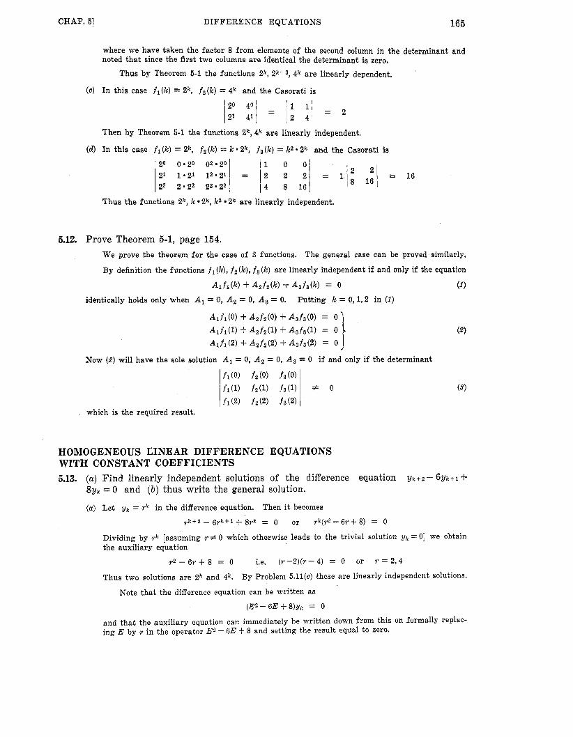
CHAP. 61 DIFFERENCE EQUATIONS 165
20 0 '20 02 20 21 1.21 12-21 = 1 22 2 '22 22-22 1
where we have taken the factor 8 from elements of the second column in the determinant and noted tha t since the first two columns are identical the determinant is zero,
Thus by Theorem 6-1 the functions 2k, 2k+3, 4k a r e linearly dependent.
( c ) In this case f,(k) = z k , f z ( k ) = 4k and the Casorati is
1 0 0 2 2 21 = 11; 1:1 = 16 4 8 1 6
Thus the functions 2k, k 2k, k2 2k are linearly independent.
5.12. Prove Theorem 5-1, page 154. We prove the theorem for the case of 3 functions. The general case can be proved similarly.
By definition the functions f l ( k ) , f 2 ( k ) , f 3 ( k ) are linearly independent if and only if the equation
A i f i ( k ) + Azf2W) + A3f3(k) = 0 (1 1 identically holds only when A , = 0, A, = 0 , A , = 0. Putting k = 0, 1,2 in (1)
HOMOGENEOUS LINEAR DIFFERENCE EQUATIONS WITH CONSTANT COEFFICIENTS 5.13. (a) Find linearly independent solutions of the difference equation y k t 2 - 6 ~ k t i +
8yk = 0 and ( b ) thus write the general solution.
(a) Let yk = rk in the difference equation. Then i t becomes
r k + 2 - 6 r k f l + 8rk = 0 or rk(r2- 6r+ 8 ) = 0
Dividing by r k [assuming r # 0 which otherwise leads to the trivial solution yk = 01 we obtain the auxiliary equation
r2 - 6 r + 8 = 0 i.e. (r -2) (r - 4) = 0 or r = 2,4
Thus two solutions a r e 2k and 4k. By Problem S. l l (c ) these a re linearly independent solutions.
Note t h a t the difference equation can be written as
(E2 - 6E 8)yk = 0
and tha t the auxiliary equation can immediately be written down from this on formally replac- ing E by r in the operator Ez - 6E + 8 and setting the result equal t o zero.

166 DIFFERENCE EQUATIONS [CHAP. 5
(b) Using Theorem 5-2, page 154, i.e. the superposition principle, the general solution is
yk = C 1 z k + C2'Ik
where c1 and c2 a r e arbi t rary constants.
5.14. (a) Find that particular solution of y k t 2 - 6ykti + 8yk = 0 such that yo = 3, yl = 2. (b) Find y5.
(a) From Problem 5.13 the general solution of the difference equation is
yk = C1zk + E2dk
Then from yo = 3, y, = 2 we have on putting k = 0 and k = 1 respectively
3 = C1 + C2, 2 = 2C1 f 4C2
from which c1 = 5, c2 = -2.
Thus the required particular solution is
yk = 592k-2 .4k
( b ) Letting k = 5 we find 765 = 5 - 2 5 - 2.45 = 5(32) - 2(1024) = -1888
The value of y5 can also be found directly from the difference equation [see Problem 5.841.
5.15. Solve the difference equation Y k t Z - 2yk.+1+ 5yk = 0.
The difference equation can be written
(E2- 2 E + 5)yk = 0
and the auxiliary equation obtained by letting yk = rk in this equation i s
r 2 - 2 r + 5 = 0
from which 2.-dF% - 2 " 4 i = 1 ' 2 i r =
2 - 2
It follows tha t solutions a r e (1 + 2i)k and (1 - 2i)k which can be shown to be linearly independent [see Problem 5.741. Since in polar form
Then the general solution can be written as
yk = 5k/2(c1 cos k s + c2 sinks)

167 CHAP. 51 DIFFERENCE EQUATIONS
5.16. Find the particular solution of the difference equation of Problem 5.15 satisfying the conditions yo = 0, 21 = 1.
Since yo = 0, y1 = 1 we have on putting k = 0, k = 1 respectively in the general solution (2) of Problem 5.15
0 = el, 1 = 51/2(c1 cos e + c2 sine)
1 from which c1 = 0, cp = I__
fi sin e
Thus
Note t h a t e can be found from (1) of Problem 5.15.
5.17. (a) Solve the difference equation Y k t 2 - 4y1,+1 + 4yk = 0 and ( b ) find the solution such that yo = 1, y1 = 3.
( a ) The difference equation can be written as (E2 - 4E + 4)yk = 0 and the auxiliary equation is
However we need another solution which is linearly independent. To find i t let yk = 2kvk in the given difference equation. Then i t becomes
v k + 2 - 2 v k + l . + v k = 0 o r A2wk = 0
rz - 4r + 4 = 0 or (Y - 2)2 = 0 so tha t r = 2,2, i.e. 2 is a repeated root.
It follows tha t Yk = rk = 2k is a solution.
Thus vk= C 1 f C p k and z/k - - 2 k ( C 1 -t C,k)
which gives the required general solution.
( b ) Putt ing k = 0 and k = 1 we find 1 = c1, 3 = 2(c, + c2)
Thus c1 = 1, c2 = 1/2, and the required solution is
5.18. (a) Solve the difference equation y k 7 3 + y k + 2 - yktl- yk = 0 and ( b ) find the solu- tion which satisfies the conditions yo = 2, y1 = -1, 3 2 = 3.
(a) The difference equation can be written as (E3 + E z - E - l )yk = 0 and the auxiliary equation is
1 3 + r z - - r - 1 = 0
This can be written a s
r*(r+ 1) - ( r + 1) = 0, (Y+ l)(r2- 1) = 0, or (r + l ) ( r+ l)(r- 1) = 0
so t h a t the roots a r e -r = -1, -1,l.
Corresponding to the two repeated roots -1, -1 we have the solution ~ ~ ( - 1 ) ~ 4- c2k( = Then by the (-l)k(~l + c&).
principle of superposition the general solution is Corresponding to the root 1 we have the solution c , ( l )k = c3.
~k = ( - l )k(~i + cnk) + ~3
( b ) Putt ing k = 0, 1 , 2 respectively we find
2 = c1 + CQ, -1 = -c1 - c2 + c3, 3 = c1 f 2c, + c3
from which c1 = $, c2 = 4, c3 = f. Thus the required solution is
yk = - 3 + ( - l )k(2k+5) 4 4

168 DIFFERENCE EQUATIONS [CHAP. 5
5.19. Find the general solution corresponding to a linear homogeneous difference equation
3, -2, -3, 3, 4. if the roots of the corresponding auxiliary equation are given by 3, - - 1f1 -C -i, -3,
2 2
Corresponding to the repeated roots 3 ,3 ,3 we have the solution 3k(c1 + c2k + c3k2).
Corresponding to the complex roots - - f - 2 i [which have polar form cos e f i s ine where 2 1 6 cos e = - i , sin e = - or e = 120° = 2 ~ 1 3 radians] we have the solution 2
2nk c4 cos ke + c5 sin ke = c4 c o s y + c5 sin- 3
Corresponding to the repeated roots -3, -3 we have the solution (-3)k(C6 + q k ) . Corresponding to the single root -2 we have the solution c8(--2)k,
Corresponding to the single root 4 we have the solution cg4k. Then the required general solution is by the principle of superposition given by
2nk 2nk 3 3 l / k = sk(c1 + c2k+ c3k2) + c4 cos- + c5 sin - + (-3)k(C6+ c7k) + C8(-2)' + c04'
METHOD OF UNDETERMINED COEFFICIENTS 5.20. Solve y k + 2 - 6yk t1 + 8yk = 3k2 + 2 - 5 ' 3 k .
The general solution of the homogeneous equation [also called complementary or reduced equation] is by Problem 5.13
u k = C 1 z k + C2qk (1 1
A1k2 + A2k + A3 (2)
Corresponding to the polynomial 3k2 + 2 on the r ight hand side of the difference equation we assume as t r ia l solution
since none of these terms occur in the complementary solution ( I )
the t r ia l solution Corresponding to the term -5 3k on the r ight hand side of the difference equation we assume
A43k (8)
Thus corresponding to the r ight hand side we assume the trial solution [or particular solution]
yk = A1k' + A2k + A3 + A43k
Substituting in the given difference equation we find
u k + 2 - 6uk+l 81/k 1 A l ( k 2)2 A2(k + 2) + A3 A43k32 - 6[A1(k + 1)' + A2(k + 1) + A3 + A43k+1]
+ 8[Alkz + A2k + A3 + A43k]
= 3Alk2 + (3A2-8Al )k + 3A3 - 4A2 - 2 A 1 - A43'
Since this must equal the r ight hand side of the given difference equation we have
3Alk2 + (3A2 - 8 A l ) k + 3A3 - 4A2 - 2 A 1 - A43k = 3k2 + 2 - 5 3k
Equating coefficients of like terms we have
3A1 = 3, 3.42 - 8A1 = 0, 3A3 - 4Az - 2A1 = 2, A4 = 5
Thus A1 = 1, A, = 813, A3 4419, A4 = 5
8 44 and the particular solution is
k2 + g k + s + 6.3'
Adding this t o the complementary solution ( I ) we find 8 44 3 9 yk = c12k + c24k + k2 + -k + - + 5 0 3 ~

CHAP. 51 DIFFERENCE EQUATIONS
t.
5.21. Solve Y k + 2 - 4 y k + l $ 4 y k = 3 ~ 2 ~ + 5 * 4 ~ . The complementary solution is by Problem 5.17
169
(1 ) c12k + c2k.2k
Corresponding to the term 3 2k on the right side of the given difference equation we would normally assume the t r ia l solution A12k. This term however is in the complementary solution (1) so tha t we multiply by k to obtain the trial solution Alk 2k. But this also is in the complementary solution (1 ) . Then we multiply by k again to obtain the trial solution Alk2*2k. Since this is not in the complementary solution (1) it is the appropriate t r ia l solution to use.
Corresponding to the term 5 * 4k we can assume the trial solution A24k since this is not in the complementary solution (1).
The t r ia l solution or particular solution is thus given by
yk = Alk2* 2k + Az4k
Substituting this into the given difference equation we find
yk+2 - 41/k+l + 4yk = A,(k+2)2*2k+' + - 4[A1(k + 1)2* 2 k f l + A,4k+l]
+ 4[A1k2*2k + A24k]
= 8A12k + 4A24k
Thus we must have 8A,2k + 4A24k = 3*2k + 5 * 4 k
5.22. Solve 9 k + 3 - 3ykt2 + 3Yk+l - y k = 24(k+2). The complementary equation is
(E3-3E2+3E- l )gk = 0 or (E- l)3yk = 0
and the complementary solution is thus
yk = C1 + c2k + ~ 3 k '
Corresponding to the term 24k + 48 on the r ight of the given equation we would normally use the trial solution Alk + Az. Since these terms occur in the complementary solution we multiply by a power of k which is jus t sufficient to insure t h a t none of these terms will appear. This is k3 so tha t the t r ia l solution is yk = Alk4+A2k3. Substituting this into the given difference equation we find
so t h a t A, = 1, A, = 2.
24Aik + 36A1+ 6Az = 24k + 48
Thus the required solution is
l/k = c1 + c2k + c3k2 + k4 + 2k3
SPECIAL OPERATOR METHODS 5.23. Let +(E) = aoEn + alEn-' + . . . + a,.
a particular solution of the equation +(E)yk = pk is given by
( a ) We have
(a) Prove that +(E)pk = +(p)pk. (b) Prove that Pk if hk = m
+(P) + 0.
Epk = p k + l = p.pk , E 2 p k = p k + 2 = pZ.pk, . . . , E n p k = p k + n = p n . p k

170 DIFFERENCE EQUATIONS [ C H A P . 5
Thus @ ( E ) p k = (aoEn + alEn-l + * + an),@
- - (a,pn -I- alp"-l + + an)pk = @(p)pk
( b ) Since @(E)pk = # ( B ) p k from par t (a) i t follows tha t
p k if G(p) + o mPk = m 1
5.24. Prove tha t 1/+(E) is a linear operator.
1 Let
-1_R,(k)= u,, ---Rp(lc) = u, 4E') d E )
Then by definition if R,(k) and R2(k) are any functions
@ ( E ) U l = R,(k) , @)U2 = R,(k) and since @(E) is a linear operator it follows tha t
d E ) [U, + U,] = R,(k) + R,(k)
1 so t h a t 4 R,(k)] = u, + UZ
or using (1) 1 1 1 [R,(k) +R,(k)] = --RR,(k) + --RR,(k) d E ) d E )
Also if 01 is any constant and R(k ) is any function let
Then
Dividing by (Y # 0 we have since +(E) is a linear operator
U = R ( k )
U or L R ( k ) = - @(E)
From (2) and (3) we have 1 1 -cuR(k) = cu-R(k)
d E ) #m) The results (2) and (5 ) prove tha t l / @ ( E ) is a linear operator.
5.25. Solve the difference equation v k t 2 - 2y, + 1 + 5yk = 2 3k - 4 * Yk. The equation can be written as (E2 - 2 E + 5)yk = 2 3k - 4 7k. By Problems 5.23 and 5.24
a particular solution is given by 1
E2 - 2 E + 5 ( 2 . 3 k - 4 . 7 k ) = 2 ' E 2 - 2 E f 5 1 3 k - 4 4 E 2 - 2 E + 5 7 k
1 3k - 4 -~ 1 I -
7' - 2(7) + 5 7 k 32 - 2(3 ) + 5 - - . 3 k - - - - 1 7 k 1 1 -
4 10 Since the complementary solution is as given in equation ( 2 ) of Problem 5.15 the required general solution is
yk = S k / 2 ( c 1 cos ke + c2 sin ke) + 3k - 2 10 7k
where 8 is determined from equation (1) of Problem 5.15.

CHAP. 51 DIFFERENCE EQUATIONS 171
Then
1 1 5.27. Prove that -pkF(k) = p k - O m +(pE) F(lc)*
Let ~ ( k ) = I F ( k ) so that @(RE) G ( k ) = F(k) . Then by Problem 5.26 d P E )
Thus
5.28. Find E2 - 4E + 2 k .
The method of Problem 5.23 fails since if g ( E ) = E z - 4 E + 4 then @) = 0. However we can use the method of Problem 5.27 with F ( k ) = 1, p = 2 to obtain
1 2 k = 2k- (1) = 2 k - 1 1 ( l ) = 2k 4Ez - 8 E + 4 ( l ) d E ) d 2 E ) (2E)Z - 4 ( 2 E ) + 4
(3k2 + 2). 1 5.29. Find E2 - 6E +
We use the method in entry 3 of the table on page 156. Putting E = 1 + A we have
(3k2 + 2 ) 1 _-
(3k2 + 2 )
(1 -I- A)2 - 6(1 -I- A ) + 8
1 3 - 4 4 + 4 2
3 1 - ($A - 442) *[I + ( $ A - & A Z ) + ( $ A - + A 2 ) 2 + * * . ] ( 3 k 2 + 2 )
( 3 k 2 + 2 ) = E2 - 6 E + 8
I -
(3k2 + 2) - 1 1 - -
=
= &[I -I- % A + ?A2 + * ] ( 3 k 2 + 2 )
=
=
= k Z + $ k + V
+[3k2 + 21 + @[3k(2) + 3k(1) + 21 + g A 2 [ 3 k ( 2 ) + 3k(1) + 21 5 [ 3 k z + 21 t $ [ 6 k ( l ) + 31 + 8 - 6 1
172 DIFFERENCE EQUATIONS [CHAP. 5
5.30. Work Problem 5.21 by operator methods. The equation can be written (E2 - 4E + 4)yk = 3 2k 4- 5 4k. Then by Problem 5.23 and
6.28 a particular solution is given by
(4k) 1
3 * E 2 - 4 E + 4 f2k) + E2 - 4 E + 4 (3 2k + 5 4k) = 3
E2 - 4E + 4
5 42 - 4(4) + 4 4k
= $k(k-l)2k + = #k(k - 1 ) 2 k + : 4k
Since the complementary solution is C12k + C2k 2k the general solution is
yk = C1zk 4 Czk 2k + #k(k - 1)2k + $ 4k
This can be written yk = C1zk f ( C ~ - # ) k * 2 ~ + 9k22k + Q * 4 k
and is the same as that obtained in equation (2) or (3) of Problem 5.21 if we take c1 = C1, cg = c, - #*
METHOD OF VARIATION OF PARAMETERS 5.31. Solve y k + 2 - 5 ? / k + l + 6yk = k2 by the method of variation of parameters.
The complementary solution, i.e. the general solution of yk+2 - 5yk+l + 6Yk = 0, is c1zk + C Z ~ ~ . Then according to the method of variation of parameters we assume that the general solution of the complete difference equation is
(1 ) yk = K12k f Kg3k
where K, and K2 are functions of k to be determined.
Since two conditions are needed to determine K, and K2, one of which is that (1) satisfy the given difference equation, we are free to impose one arbitrary condition. We shall choose this condition to be that the sum of the last two terms in (2 ) is identically zero, i.e.
2kflAK1 +3k+lAKZ = 0 (3)
so that (2) becomes AYk - - Kl2k + K22.3'
Now the given equation can be written as
(E2- 5E + 6)yk = k2 . (6)
(A2734 + 2)yk = kz (7) or since E = 1 + A
Using (I), ( 4 ) and (5 ) in (7) we find after simplifying
2k+1AK1 + 2*3k+lAK2 = k2
We must thus determine K1 and K2 from the equations (3) and (8), i.e.
2k+lAK1 + 2*3k+lAK2 = k2
2kt1AK1 + 3k+lAK2 ( 9 )
Note that these equations could actually be written down directly by using equations (24) on page 157.

173 CHAP. 51 DIFFERENCE EQUATIONS
Then
These can be obtained by using the methods of Chapter 4 or the operator method of Problem 6.27. Using the la t ter we have, omitting the arbi t rary additive constant,
K 1 = -:(&) = - A ( & ) k ( F ) E - 1
Thus taking into account a n arbi t rary constant cl,
K 1 = $ ( k z + 2 k + 3 ) + c1
Similarly we find K 2 = -- ( k 2 + k + 1 ) + c2
2 3 k
Then using these in (1) we find the required solution
v k = C 1 z k + C23k + &k2 + $ k Q
METHOD OF REDUCTION OF ORDER 5.32. Solve y k t 1 - ryk = Rk where r is a constant.
Method 1, using variation of parameters.
The complementary or homogeneous equation corresponding to the given equation is
Y k + l - ryk =
From this we find
y k = ‘rVk-1, y k - 1 = rZ/k-zr ... 1 Y2 = ryll 111 = ‘Yo
so tha t the solution of (1) is 76k = rkyO or y k = cork
where we take co = yo as the arbi t rary constant.

174 DIFFERENCE EQUATIONS [CHAP. 6
We now replace co by a function of k denoted by K ( k ) , i.e.
yk = K(k)rk (2)
and seek to determine K ( k ) so that the given equation is satisfied. Substitution of (2) in the given equation yields
or dividing by r k + l ,
K ( k + l ) r k + l - K(k)rk+l =
K ( k + 1) - K ( k ) = AK =
Rk
Rk y k + l
Thus K = A-1 (&) and so from (2)
Method 2, multiplying by a suitable summation factor.
Multiplying the given equation by llrk+l it can be written as
Thus
or
where c is an arbitrary constant, The factor l l r k + 1 used is called a summation factor.
5.33. Solve y k t 2 - 5yk+l+ 6yk = k2 by the method of reduction of order.
Write the equation as (E - 3)(E - 2)yk = k2. Letting Zk = (E - 2)yk we have
(E-3)Zk = k2
Then by Problem 5.32 the solution is
Thus (E - 2)yk = C13k - +(k2 k + I )
Applying the method of Problem 5.32 again the solution is
= &k' + 4 k + 8 + ~22' + ~33k
We can use the method to find particular solutions by omitting the arbitrary constants.
METHOD OF GENERATING FUNCTIONS 5.34. Solve the difference equation
y k + 2 - 3 Y k + l +2yk = 0 if yO=2, y 1 = 3
by the method of generating functions. m
Let G(t ) = x 2/ktk. Multiplying the given difference equation by tk and summing from k=O

CHAP. 51 DIFFERENCE EQUATIONS 175
Putting yo = 2, yl = 3 in (1) and solving for G ( t ) we obtain
2 - 3 t - 2 - 3t 1 - 3t + 2 t 2
- (1 - t)(l - 2 t ) G(t ) =
Writing this in terms of partial fractions we find
G(t) = - 1 + 2 = 5 t k + 5 ( 2 t ) k = ( 1 + Z k ) t k k=O k=O k=O 1-2t 1-22t
Thus 5 V k t k = 5 (1 + 2 k ) t k k = O k=O
and so y k = 1 + zk which can be verified as the required solution.
LINEAR DIFFERENCE EQUATIONS WITH VARIABLE COEFFICIENTS 5.35., Solve the first order linear difference equation with variable coefficients given by
Z / k + i - Ak'& = R k O r ( E - A k ) Z / k = R k .
Method 1, using variation of parameters. The complementary or homogeneous equation corresponding to the given equation is
? d k + l - A k ? d k = 0 (1 1 From this we have
Y k = A k - 1 % - 1 , y k - 1 = A k - 2 y k - 2 , 9 yz = A l y l
so that the solution of (1) is ?dk = A k - i A k - 2 . * ' A ~ y i
or Y k = ~ 1 A 1 A 2 . * * A k - 1
where we take c1 = yl as the arbitrary constant.
We now replace c1 by a function of k denoted by K(k) , i.e. ~k = K(k)A,Az* * ' A k - 1 (2 )
Substitution of (2) in the given and seek to determine K ( k ) so that the given equation is satisfied. equation yields
K(k + 1 ) A I A 2 * * ' A k - A k K ( k ) A , A , . * A k - 1 = R k
Thus
and so from (1) we find the required
?dk =
= AlA2*
where c is an arbitrary constant.
solution

176 DIFFERENCE EQUATIONS [CHAP. 6
Method 2, multiplying by a suitable summation factor.
Multiplying the given equation by l IA ,AZ-**A, i t can be written
or
Then
or
w e call 1/AlA2* * * A k used to multiply the given equation the summation factor.
5.36. Show that the equation y k + 2 - ( k + 2 ) y k + l + k y k = k can be written in the factored form (E - A k ) ( E - B k ) Y k = k.
The given equation is in operator form
[E2 - ( k + 2)E + k ] y k = k
Let us t r y to determine Ak and Bk so tha t (2) is the same as
(E - Now the lef t side of ( 2 ) can be written a s
- B k ) Y k = k
( E - A k ) ( Y k + l - B k Y k ) = ?dk+Z - B k + l Y k + l - A k ( y k + l - B k Y k )
= y k + 2 - ( A k + B k + l ) ? d k + l + A k B k Y k
Comparing with the left side of the given equation (1) we have
A k + B k + l = k + 2 , A k B k = k (4 From the second equation of (8) we are led to t ry either A k = k , B k = 1 or A k = 1, B k = k. Since the second set, i.e. A k = 1, Bk = k , satisfies the first equation of (3) the given equation Can be written as
(E - 1)(E - k ) Y k = k
5.37. Sohe Y k + ? - ( k i - 2 ) Y k + l + k y k = k , Y l = o , Y Z = 1 . By Problem 5.36 the equation can be written as
(E - 1)(E - k ) y k = k
Let xk = (E - k )yk . Then (2) becomes ( E - l ) ~ k = k
which has the solution k ( 2 ) zk = ~ - 1 k = A - l k ( 1 ) = - 2 + 01
k ( 2 ) Then ( E - k ) y k = 2 + C1 = + k ( k - 1 ) + C1
By Problem 5.35 this has the solution
or

177 CHAP. 51 DIFFERENCE EQUATIONS
From yl = 0, y2 = 1 and the difference equation we find, if k = 1, y3 - 32/2+ g1 = 1 y3 = 4.
SO that If we put k = 2 and k = 3 in (S), we find using O! = 1
C 1 + C 2 = 1, 1 + 3C1 + 2C2 = 4
from which c1 = 1, c2 = 0. Thus the required solution is k -1 1 + ( k - l ) ! 2 - p = 1 P !
2/k = - 2 p=1
This can be written for
g k = Wql 2 +
k > 3 as
(k - l ) ! l + - + F + 1 1 . ' . +'-I + ( k - l ) ! 2 ! ( k - 3) !
5-38, Solve ( k + l ) y k + Z - (3k +2)gk+1 + (2k- 1)yk = 0.
The equation can be written as
( k + 1)A22/k - kAYk - 22/k = 0
Assume a solution of the form 4
2/k 2 Cpk(p) p =-m
where we take cp = 0 for p = -1, -2, -3, . . .
From (2) we obtain m
- x pcpk(P--l) - p = - - o o
Substituting (Z), (4 ) and ( 5 ) into (I), i t becomes
2 p ( p - 1)Cpkk(P--2) + 2 p ( p - l)Cpk(P--P) - 2 pc,kk(p-') - 2~,k(p) = 0 (6)
where we have omitted the limits of summation. On using the result
kk(rn) = k(rnt1) + mk(rn)
(6) can be written
2 p ( p - l )cp[k(P- ' ) + ( p - 2)k(P-2)] + 2 p ( p - 1)Cpk(p-2)
- 2 pc,[k(P) + ( p - l )k(p-1)] - 2 2cPk(p) = 0
This in turn becomes on collecting coefficients of k(p)
2 { ( p + 2)(p + 1)2cp+, - (P + 2 ) c p W ) = 0 (7)
Since (7) is an identity each coefficient must be zero, i.e.
(P + 2 ) ( P + W p + 2 - (P + 2)cp = 0
Using (3) it follows that we must have p = 0,1,2, . . . so that (8) becomes on dividing by p + 2 P 0
(p+1)2cp+2 - cp = 0 ( 9 )
Putting p = 0,1,2, . . . in (9) we find
12cz - co = 0, 22c3 - c1 = 0, 32c, - c* = 0 , 42c, - cs = 0, . . . r.

178 DIFFERENCE EQUATIONS [CHAP. 5
STURM-LIOUVILLE DIFFERENCE EQUATIONS 5.39. Prove that the eigenfunctions +m,k, +n,k belonging to two different eigenvalues Am,
An satisfy the orthogonality condition N c rk+m,k+n,k =
k = l
Since Am, @m,k and An, @n,k are the corresponding eigenvalues and eigenfunctions they must by their definition satisfy the equations
A(Pk- 1 A@m, k- 1) + (qk + Amrk)@m, k (1)
A(pk- [email protected] l ) + (qk + Anrk)@n,k = (2 )
=
for k = 1, , . ., N .
If we multiply these equations by @n,k and @m,k respectively and then subtract we find
(Am - An)rk @m, k @n,k = @m, k A[pk- IA@n, k- 11 - @n, k A b k - 1 ‘@m, k- 11 (3)
Summing from k = 1 t o N then yields
Using summation by parts this can be written N N + l
(Am--n) k = l 3 r k @ m , k @ n , k = P k - l [ @ m , k A @ n , k - l - @n,[email protected] l ] /k=l
= PN[@m, N + 1 A@n,N - @n, N + 1 A@m, NI
- Po[Cm,lACn,o - @ n , ~ A @ m , o l
- Po[@,, o@n, 1 - Gn, 0, Cm, 11
= PN[@m, N@n, N + 1 - @n, N@m, N + 11 ( 4 )
From the boundary conditions (34), page 158, which must be satisfied by @m,k and @n,k we have
aO@rn,O + a l @ m , l = 0, aN@m,N + U N + l @ r n , N + l =
“O@n,O f a l @ n , l = 0, aN@n,N + a N + l @ n , N f l =
By eliminating a0, al, ah,, a N + l from these equations we see that they are equivalent to
‘$rn,O@n,l - @n,O@m,l = 0, @m,N@n,N+l - @n,N@m,N+l =
Using these in ( 4 ) we thus have N
k = l (Am- Ax,) 2 rk@m,k@n,k = 0
and if Am # An we must have as required N
2 rk@m,k’&,k = k = l

CHAP. 51 DIFFERENCE EQUATIONS 179
5.40.
5.41.
Prove that if p k , q k , r k in equation (33), page 158, are real then any eigenvalues of the Sturm-Liouville system must also be real.
eigenfunction which may be complex. Suppose that Am is a n eigenvalue which may be complex and that @m,k is the corresponding
Then by definition,
A ( P k - lA@rn,k- l ) + ( q k + Amrk)@m,k = 0
A ( p k - l A $ m , k - l ) + ( q k + L r k ) z m , k = 0
(1 1 Taking the complex conjugate of this equation [denoted by a bar over the letter] we have
(2) using the fact tha t Pk-1 , qk, Tk a r e real.
&,k and then subtracting, we find [compare equation (3) of Problem 5.391 By proceeding as in Problem 5.39 multiplying the first equation & k , the second equation by
- N x r k @ m , k @ m , k = 0 k = l
or N
= o - -
Since r k > 0, the sum in (3) cannot be zero and so we must have X, - Am = 0 or A, = A,, i.e. Am i s real.
N
Let F k = c,&,~ where +m,k are the eigenfunctions of the Sturm-Liouville m=l
system on page 158 assumed to be real.
(a) Show that formally N
k = l c rkFk+m,k
m = 1,. . . , N - Cm - N
( b ) What limitations if any are there in the expansion obtained in part (a)? N
then multiplying both sides by rk@n,k and summing from k = 1 to N we have N N N
3 r k F k @ n , k = x 2 C m r k @ m , k ' h , k k = l k = l m = l
N
= m = l 2 cm{k$l rk@m,k@n,k
N
where we have used the fact tha t N
3 r k @ m , k @ n , k = m S ; n k = l
by Problem 5.39. We thus have N
rkFk&,k k = l
N cn =
3 rk@?t,k k = l
which i s the same as the required result on replacing n by m. For the case where the eigenfunctions may be complex see Problem 5.129.

180 DIFFERENCE EQUATIONS [CHAP. 5
(a) In order to understand the limitations for the expansion in (a) it is useful to use the analogy of vectors in 3 dimensions as indicated on page 159. In 3 dimensions i, j, k represent unit vectors. If we wish to expand an arbitrary 3-dimensional vector in terms of i, j, k we seek constants A,, A2, As such that
A = A l i + A j + A s k
We find Al = A - i , A, = A * j , A, = A * k
as the solution of this problem.
Now if the only vectors given to us were i and j [with k not present] it would not be possible to expand the general 3-dimensional vector A in terms of i and j, i.e. we could not have
A = A , i + A z j
We say in such case that the set of unit vectors i and j are not a complete set since we have in fact omitted k.
In an analogous manner i t is necessary for us to have a complete set of eigenfunctions in order to be able to write the expansion in (a).
5.42. Illustrate the results of Problems 5.39-5.41 by considering the Sturm-Liouville system
A’Yk-1 + X Y k = 0, YO = 0, YN+1 = 0
The system is a special case of equations (38) and (34) on page 168 with
p k - 1 = 1, qk = 0, T k = 1, “0 = 1, “1 = 0, “N = 0, “Ni-1 = 1
The equation can be written ? d k + l - (2-1)yk + yk-1 = 0
Letting yk = rk we find that r 2 - (2 - 1)r + 1 = 0
so that 2 - h -C q ( 2 - k p - 4
2 r =
It is convenient to write 2 - A = 2 c o s e
so that (2) becomes
Then the general solution of the equation is
r = cos B * i sine
yk = 01 COS ke + C 2 sin kO
From the first boundary condition yo = 0 we have c1 = 0 so that
yk = c2 sin ke
From the second boundary condition yNt l = 0 we have since C , Z 0
sin ( N - t 1)s = 0
From this we h a d nn
N S 1 ( N + l ) e = nr or 6 = - n = 1 , 2 , 3 , .
(5 )
(7)
where we have omitted n = 0 since this leads to the trivial solution yk = 0 and we have omitted n = -1, -2, -3, . . . since these lead to essentially the same solutions as n = 1,2 ,3 , . . . From (3) and (8 ) we see that
n = 1,2 ,3 , . . .

CHAP. 61 DIFFERENCE EQUATIONS 181
Since these values start to repeat after n = N , there will be only N different values given by
n7; A,, = 4 sin2- 2(N + 1) n = 1,2, . . .
These represent the eigenvalues of the Sturm-Liouville system. are obtained from (6) as
The corresponding eigenfunctions
kna c2 sin - N + 1
From the orthogonality property of Problem 5.39 we would have N krn% kna B sin ~ sin- = 0 m # n
k=l N + 1 N S 1
which can in fact be shown directly [see
Similarly if we are given a function
where c, =
Problem 5.131(a)].
Fk we can obtain the expansion N krnp = B c, sin -
m = l N + l
These can also be shown directly [see Problem 5.131(b),(c)].
NONLINEAR DIFFERENCE EQUATIONS 5.43. Solve y,,, - y, + ky,+,y, = 0, y1 = 2.
Dividing by Y k l / k + l , the equation can be written as
1 1 = k Y k + l Y k
Then letting = wk the difference equation to be solved is
' v k + l - w k = k, v1 = 4 The solution to the linear difference equation in (2) is
and using the fact that w1 = 4 we find c1 = &. Thus
k (k - 1) 1 k 2 - k k l 2
- + - = 2 2 W k =
and the required solution is 2
= k Z - k + 1
5.44. Solve y,+,yi = yE+l if y1 = 1, yz= 2.
Taking logarithms of the given difference equation it becomes
lnyk+2 - 3lnyk+1 + 21nYk = 0
Letting Vk = h g k
the equation (1) can be written as a linear difference equation
w k + 2 - 3 2 ) k + l + 2vk = 0, 211 = 0, VUg = In 2
The general solution to the difference equation in (3) is wk = c1 + CZZk

182 DIFFERENCE EQUATIONS
Using the conditions in (3) we find c1 = -In 2, c2 = 4 In 2 so that
'vk = (In 2)(2k--1- 1)
The required solution of the given difference equation is thus
In yk = (In 2)(2k--1- 1) ( l n 2 ) W - l - 1) yk = e or
p k - 1 - 1 which can be written yk = 2
[CHAP. 5
SIMULTANEOUS DIFFERENCE EQUATIONS
8 k + l +'k - 3yk = k subject to the conditions y1 = 2, z, = 0.
38, + - 52, = 4 k 5.45. Solve the system
Operating on the first equation in (1) with E - 5 and leaving the second equation alone the system (1) can be written
($1 (E - 5)(E - 3)yk (E - 5)Zk = 1 - 4k
3yk f (E-5)Zk = 4k
Subtracting the equations in (2 ) yields (E2 - 8E + 12)yk = 1 - 4k - 4k
The general solution of (3) found by any of the usual methods is
1 4 19 5 26 u k = C 1 z k + ~26k + dk - -k - -
and so from the first equation in (1) 1 3 34 c12k - 3c26k - - 4k - - k - - 4 6 26 zk =
Putting k = 1 in ( 4 ) and (5 ) we have since 111 = 2, z1 = 0
64 25 ' 2 ~ 1 + 6 ~ 2 = -
from which c1 = 133/100, c2 = -1/60.
Thus the required solution is
74 201 - 18c2 = 25
133 1 4 19 100 60 5 25 uk = -2k - -6k + 4k-l - -k - -
133 1 3 34 100 20 5 25 zk = -2k + -6k - 4k-l - -k - -
MIXED DIFFERENCE EQUATIONS 5.46. Solve the diff erential-diff erence equation
y;+~(~) = yk(t)t = t> Z/k(O) = Putting k = 0 we find
tz y ; ( t ) = yo( t ) = t or y l ( t ) = F + c1
Then since ~ ~ ( 0 ) = 1, we have c1 = 1 so that

CHAP. 51 DIFFERENCE EQUATIONS 183
Putting k = 1 we find
t 2 t3 d(t) = y l ( t ) = 1 + 2 or y 2 ( t ) = t + 3 + c2
Then since yz(0) = 2, c2 = 2 so that
t 3 3!
y z ( t ) = 2 + t + - Continuing in this manner we find
t 2 t 4
2 ! y3(t) = 3 + 2t + - + 2 tz t 3 t 5
y4(t) = 4 + 3t + - + - + - 2 ! 3 ! 5 !
y5(t) = 5 + 4 t + - + 3 + + + g 3t2 2t3 t 4 t 6
2 ! and in general
(n - 2)t2 (n - 3)t3 tn-1 t n t l +-+- 2 ! 3! ( n - l ) ! ( n + l ) ! y , ( t ) = n + ( n - l ) t + - + - + ...
which is the required solution.
5.47. Solve Problem 5,46 by using the method of generating functions. Let the generating function of yk( t ) be
00
y(s , t, = 3 Y k ( t ) s k k=O
Then from the difference equation,
which can be written in terms of (1) as
or since yo(t) = t - - ;; SY = 1
Putting t = 0 in ( 1 ) and using y k ( 0 ) = k yields Lo
Y(s,O) = 3 ksk k=O
Equation (4 ) can be written as
i a s a t --In ( sY+ 1) = 1 or l n ( sY+ 1) = s t + c1
Y(s, t ) = - ceSt - 1 6
so that
Using (5 ) and (6) we find
Y(s , t ) = A{& 8 ( 1 + k=O k s k + l ) - l }

184 DIFFERENCE EQUATIONS [CHAP. 6
Since the coefficfent of 8n in this expansion is y n ( t ) we find i t t o be
This i s obtained by taking the term corresponding to p = n + 1 in p + k + 1 = n + 1 in the second summation of (7).
(8)
the first summation of (7) and
The required solution (8) with n replaced by k agrees with that of Problem 5.46.
PARTIAL DIFFERENCE EQUATIONS 5.48.
5.49.
Write the partial difference equation u(x + h, y) - 4u(z, y + I ) = 0 the operators El, E2 and ( b ) in terms of subscript notation.
(a) in terms of
Solve the difference equation of Problem 5.48.
We can write equation (2 ) of Problem 6 . 4 8 as
E1uk,m = 4EZUk,m (1 1 Considering m as fixed (1) can be thought of as a first order linear difference equation with constant coefficients in the single variable k. Calling U k , m = u k , 4E2 = a the equation becomes
Euk = auk (8)
Uk = akC (8) A solution of (2) is
where C is an arbitrary constant as f a r as k is concerned but may depend on m, i.e. it is an arbitrary function of m. We can thus write (8) as
u k = akCm (4)
Restoring the former notation, i.e. u k = uk,m, a = 4 E 2 , (4 ) becomes
Uk,m = kc, But this can be written as
U k , m = 4kE:Cm = 4 k C m + k (5 )
Then (5) To obtain this in terms of x and y we use the fact that x = a + kh, y = b + ml. becomes
u ( x , y ) = 4(z--a)lhC c + y - 6 ) ( h 1
( h J which can be written
u(s,y) = 4*/hH 'f (6)
where H is an arbitrary function.
We can show that (6) satisfies the equation of Problem 5 . 4 8 . arbitrary function it is the general solution.
Then since it involves one

186 CHAP. 51 DIFFERENCE EQUATIONS
5.50.
5.51.
5.52.
Work Problem 5.49 by finding solutions of the form Akpm where A, p are arbitrary constants.
Substituting the assumed solution Uk,m = Akam
in the given difference equation (2) of Problem 5.48 we find
),k+lpm- 4),kpm+l = 0 or A - 4p = 0
on dividing by hkpm # 0.
From A = 4p it follows that a solution is given by
Akpm = (4p)kpm = 4kpk+m
Since sums o f these solutions over any values of p are also solutions, we are led to the solutions
where F is an arbitrary function. Thus we are led to the same result as given in Problem 5.49 where the arbitrary function F(k + m) = Ck+m.
Solve u(x + 1, y) - 4u(x, y + 1) = 0, u(0, y) = y2. The difference equation is the same as that of Problem 5.48 with h = 1, 1 = 1. Thus the
general solution is from equation (6) of Problem 5.49,
u ( x , y ) = 4 W ( z + y ) (1 )
Using the boundary condition u(0 , y) = y2 we have from (1)
U(0,Y) = H(y) = ?d2
Thus H ( x + y ) = (x+y)2
and the required solution is u ( x , y ) = 4=(x+y)2 (8)
Solve u(x + 1, y) - 2u(x, y + 1) = 3u(x, y).
We can write the equation in subscript notation as
E I U k , m - ~ E Z U ~ , ~ = 3Uk,m or (E i -2E2-3 )uk ,m = 0
Rewriting it as ElUk,m = ( 2 E Z + 3)Uk.m
we can consider i t as a first order linear difference equation with constant coefficients as in Prob- lem 5.49 having solution
uk,m = (2Ez + 3)kCm
This can be written as U k , m = 3k(l++Ez)kCm
or on expanding by the binomial theorem,
= 3k[C, + $kCm+l + $ k ( k - l ) C m + z + & k ( k - l ) ( k - 2 ) C m + , + a * * ]
To obtain the result in terms of x and y we can use x = a + kh , y = b + ml, choosing h = 1, 1 = 1, a = 0, b = 0 so that k = x, m = y. Then writing Cm = H ( y ) we obtain
U ( X , 2/) = 35[H(y) + Q x H ( y + 1) + $X(X - 1)H(y + 2) + &X(X - l ) ( ~ - 2 ) H ( y + 3 ) + * * a ]
This contains one arbitrary function H ( y ) and is the general solution.

188 DIFFERENCE EQUATIONS [CHAP. 5
MISCELLANEOUS PROBLEMS 5.56. Solve the partial differential equation
dU dU - + 2 - = 0, U ( X , 0 ) = x3 - 3 sinx dX dY
The given partial differential equation is the limit as h -+ 0, 2 -+ 0 of
u(x + h, - u(z, 7 d ) h
which can be written in operator and subscript notation as
(ZE, + 2 h E 2 - 1 -2h)uk , , = 0 or E ~ . L I ; , ~ = 14- -- - E 2 U k , m ( ) This can be solved as in Problem 5.49 t o yield
or in terms of x and g as
u(x,y) = (1 + ~ - T E ~ ) 2h 2h 'Ih H ( Y )
In order to obtain meaningful results as h -+ 0, I -+ 0 choose 1 + 2h/l = 0 so that (1) becomes
u(x,y) = H(+ y - 2x = 4 2 % - y)
where J is an arbitrary function. The required general solution is thus
u(x,v) = J ( 2 x - v )
Since
we have
u ( ~ , 0) = J ( 2 x ) = x3 - 3 sin x
J(x) = &x3 - 3 sin (xl2)
( 2 x - Y\ \ 2 )
Then from (2) we have u ( x , y ) = 3 2 % -y)s - 3 sin -
5.57. Solve the mixed difference equation dU u(x + 1, y) - u(x, y) = 2- dY
The given equation can be written as
E1u-u = 2DZu (1 )
o r E,u = ( 1 + 2 D 2 ) u ( 2 )
2@,2/) = (1 + 2D,)"H(v) (3)
Then treating l + 2 D 2 as a constant we find as in Problem 5.49
where H ( y ) is an arbitrary function of y. Expanding by the binomial theorem we then find
Then if x is a positive integer the series terminates and we have
u(x,u) = H ( y ) + 2 (3 H'(y) + 22 (i) H"(y) + - * * + 2" H(")(y) ( 4 )

CHAP. 61 DIFFERENCE EQUATIONS 189
5.58. Solve the preceding problem subject to u(0,y) = y3.
U(0,Y) = H(y) = Y3
From ( 4 ) of Problem 6.67 we see that
Thus H’(y) = 3y2, H”(y) = 6y, H”’(y) = 6, H(Iv)(y) = 0, ,
and so
5.59. Find the general solution of u k , m = p U k t 1 , m - 1 + q U k - l , m + l
where p and q are given constants such that p + q = 1.
Method 1. Assume a solution of the form
%k,m = Xkpm
Then by substitution in the given difference equation we find after dividing by A k p
p x 2 - x p + q p 2 = 0
from which P * m - - P * P d i = G l = p , c l Q
2 P x =
2 P
Thus solutions are given by p k * pm = pktm and ( p q / p ) k p m = p k t m ( q / p ) k . Since sums of such solutions are also solutions, i t folIows that F ( k + m ) and (q/p) lCG(k+m) are solutions and the general solution is
(1) %k,m = F ( k + m) + ( q / p ) k G ( k + m)
where F and G are arbitrary functions.
Method 2.
denote this by c we have k + m = c. It is noted that the sum of the subscripts in the given difference equation is a constant. If we
The equation is thus given by
U k , c - k = P U k t l . c - ( k t l ) f q U k - l l , c - ( k - l ) (2)
If we let U k , c - k = vk
(2) becomes v k = p v k t 1 f q v k - 1
which involves only one subscript and can be solved by the usual methods. We find
v k = c1 + C Z ( q / I ) ) ‘ ( 5 )
Now the constants c1 and c2 can be considered as arbitrary functions of the constant c = k + m: c1 = F(k+m), c2 = G ( k + m ) . Thus we obtain from (8) and ( 5 )
U k , m = F(k + m) + G(k + m)(q/p)k

190 DIFFERENCE EQUATIONS [CHAP. 5
Supplementary Problems DIFFERENTIAL EQUATIONS AND RELATIONSHIPS TO DIFFERENCE EQUATIONS 5.60. ( a ) Show t h a t the general solution o f the differential equation
is y = c e ~ - x 2 - 2 x - 2 .
( b ) Find t h a t particular solution to the equation in ( a ) which satisfies the condition y(0) = 3.
5.61. ( a ) Show t h a t the equation
[compare Problem 5.601 where y = f(x), Ax = h can be written as
f(x + h) - (1 + h)f(x) = hx2 - h2x
( b ) Show t h a t the general solution of the equation in (a) is y(x) = f (x) = C(x)(l + hp’h - x2 + ( h - 2)x - 2
where C(x + h) = C(x) .
(c ) Find t h a t particular solution for which y(0) = 3.
5.62. Explain clearly the relationship between the difference equation and the differential equation o f Problems 5.60 and- 5.61 discussing in particular the limiting case a s h + 0.
5.63. ( a ) Show t h a t the general solution of
3x2 - 5x + 4
i s y = c1 cos x + c2 sin x + 3x2 - 5% - 2.
( b ) Find t h a t particular solution to the equation in (a) which satisfies the conditions y(0) = 2, Y’(0) = 0.
5.64. (a) Show t h a t the equation - “16 + 16 = 3x(2) - 5x(1) + 4 Ax2
can be written as
f(x + 2h) - 2 f ( x + h) + (1 + h2)f(X) = 3h222 - (3h3 + 5h2)x + 4h2
where y = f(x).
( b ) Show t h a t the general solution o f the equation in (a ) is
y = f (x) = Cl(X)(l+ ih)”/” + C,(x)(l- ih)”/h + 3x2 - (3h + 5)x - 2 where Cl(x) and C2(x) a re periodic constants with period h.
“ 5.65. (a ) Explain clearly the relationships between Problems 5.63 and 5.64, in particular the limiting
case as h + 0. (21) What a re the boundary conditions for the difference equation in Problem 5.64 which correspond to those for the differential equation in Problem 5.63? (c) Obtain the particular solution of Problem 5.64 corresponding to the boundary conditions just found in ( b ) , and explain the relationship between this and the particular solution of Problem 5.63.
THE SUBSCRIPT NOTATION FOR DIFFERENCE EQUATIONS 5.66. Write the difference equation of ( a ) Problem 5.61 and ( b ) Problem 5.64 with subscript notation.
5.67. Write each of the following in subscript notation.
( a ) f (x + 3h) - 3f(x + 2h) + 3f(x + h) - f(x) = x(3) - 2392)
( b ) f ( x + 4 h ) + f(x) = cosx

CHAP. 51 DIFFERENCE EQUATIONS 191
5.68. Change each of the following equations to one involving the “ x notation”.
(a) 2 Y k t 2 -3 ldk+l+yk = 0 ( b ) yk+3 + 4Ykt2 - 52/k+l + 211; = k2 - 4k + 1
LINEARLY INDEPENDENT FUNCTIONS 5.69. Determine which of the following sets of functions are linearly dependent and which are linearly
independent. (a) 2k, k - 3 ( e ) 1, k, kz, k3, k4 ( b ) k + 4, k - 2, 2k + 1 ( 0 ) k2 - 2k, 3k, 4 (8 ) 2k cos ke, 2k sin ks (d ) 2 5 225 23k (h) k2, (k + 1)2 , (k + 2)2, (k + 3)2
(f) k2 - 3k + 2, k2 + 5k - 4, 2k2, 3k
5.70.
5.71.
Work Problem 5.69 using Theorem 5-1, page 154.
Show that if 0 is added to any linearly independent set of functions then the new set is linearly dependent.
Prove Theorem 5-1, page 154, for any number of functions. 5.72.
5.73.
5.74.
Prove Theorem 5-2, page 155.
If a # b show that a k and bk are linearly independent.
5.82. Find the general solution corresponding t o a linear homogeneous difference equation if the roots of the corresponding auxiliary equation are given by 2, -2, -3 * 4i, -2, -2, 4, -2, 2.
What is the difference equation of Problem 5.82?
Work Problem 5.14(b) directly by using the difference equation.
5.83.
5.84.
P

192 DIFFERENCE EQUATIONS [CHAP. 5
5.86. Solve & + I - a u k = p for all values of the constants (Y and p.
5.93. Show that (a) - coske = Re (b) sinke = Im {-I dE)
where Re denotes “real part of” and Im denotes “imaginary part of”.
5.94. Use Problem 5.93 t o solve yk+2 + 4uktl - 122/k = 5 cos ( d 3 ) .
5.95. (a) Determine E R ( k ) . 1
1 1 = - (y - L, i.e. the method of partial fractions can be 1
used for operators.
(c ) Show how the results of (a) and ( b ) can be used to solve the equation
( b ) Show that E2- 6 E + 8 2 E 4 E - 2
2/k+2 - 61/k+l + 816k = k2 + 3k
5.96. Show how operator methods can be used to solve (E - 1)2(E + 2)(E - 3)uk = kz - 3k f 5 + 3k
5.98. Solve Problem 5.86(a)-(i) by operator methods.
5.99. Solve (a) Problem 5.87, (b) Problem 5.88, ( c ) Problem 5.89, (d) Problem 5.90 and (e) Problem 5.91 by operator methods.
METHOD OF VARIATION OF PARAMETERS 5.100. Solve each of the following difference equations by using the method of variation of parameters.
(a) u k + 2 - b k t l f 6?dk = k2 (b) ( c )
(d) u k t 2 f ?dk = ( e ) (f) Y k + 2 - 1 / k t l + 1 6 k = l/k!
v k + 2 - 2yk+l f u k
41dkt2-41dkt1 + u k = 3/2k
= 3 + k + 4k
5Yk+2 - 3 Y k t l - 2uk = 3k + (-2)k

CHAP. 51 DIFFERENCE EQUATIONS 193
5.101. Solve Problem 6.86(a)-(i) by using variation of parameters.
5.102. Solve Problem 5.92(a)-(It) by using variation of parameters.
5.103. Solve l/k + 3 - 676k + 2 + 1176, + 1 - 676k = 5 2k + kz by using variation of parameters.
5.104. Verify t h a t the determinant of the coefficients (24) on page 157 is equal to the Cmorat i of the system [see (Is) , page 1541. Discuss the significance of the case where the determinant is or i s not zero.
METHOD OF GENERATING FUNCTIONS 5.105. Verify each of the following generating functions.
5.106. Solve each of the following by the method of generating functions.
(a) 7 6 k t 2 - 62/k+i 8 Y k = 0, Yo = 0, 761 = 2 ( b ) 276k+l - 76k = 1, 760 = 0, (c)
(d )
( e ) (f) (9) Y k t 2 + 276k+l + 76k = + (h)
Y k t 2 + 476k+l + 476k = 0, 676k+Z - 5yk+l + 76k = 76k+2 + 21/k+l f 76k = 0, 76k+3-376k+2 + 376k+1 - Yk =
760 = 1, 761 = 0
760 = 2, 761 = -1
476k+2 - 476k+l + 76k = 2-', 760 = 0, 761 =
1 5.107. Solve g k + 2 + 376k+1 - 476k = z, 760 = 0, 761 = O.
5.108. Show how to obtain the generating function of the sequence (a) uk = k, ( b ) uk = k2, (C) uk = k3.
[Hint.
If G(t) and H ( t ) a r e the generating functions of uk and vk respectively show tha t G(t)H(t) is the
Use Problem 6.105(a) and differentiate both sides with respect to t.]
5.109. generating function of k
u:vk = Uk-pvp g=O
which is called the convolution of uk and V p

194
5.112.
5.113.
5.114.
5.115.
5.116.
5.117.
5.118.
5.119.
5.120.
5.121.
5.122.
5.123.
5.124.
5.125.
DIFFERENCE EQUATIONS [CHAP. 5
Work Problem 5.113 if the right side is replaced by 2k, using variation of parameters.
Let Yk f; 0 be any solution of the difference equation
Y k + 2 + akyk+l + bkyk = 0 Show t h a t this second order linear difference equation can be reduced to a first order linear dif- ference equation by means of the substitution yk = YkUk and thus obtain the solution.
Show tha t if Yk is a solution of the equation
Y k + 2 + ak?dk+l + bkyk = 0 then the substitution yk = Ykuk can be used to solve the equation
Y k + 2 + a k Y k + i + bkYk = Rk
Use Problems 5.117 and 5.118 to solve the equations
(a) kyk+2 (1 - k)Yk+l - 276k = 0 (b) h k + 2 f (l--k)Yk+l - 2Yk = 1 [Hint. A solution of (a) is yk=k.]
Discuss the relationship of the methods of Problems 5.117 and 5.118 with the method of varia- tion of parameters.
Solve
Solve ak+2ykt2 - (aak+l f bk+1)2/k+l + a b k Y k = where CY i s a given constant.
Solve yk+z + kyk = k, yo = 0, yl = 1 by the method of generating functions.
Solve Problem 5.116 by the method of generating functions.
(a) Solve Problem 5.37 by making the substitution yk = (k - I)! 'uk. (b) Show tha t lim yk = # e . k-co
STURM-LIOUVILLE DIFFERENCE EQUATIONS 5.126. Find eigenvalues and eigenfunctions for the Sturm-Liouville system
A'Yk-1 + ?i& = 0, Y l = YO! Y N + l = U N
5.127. Work Problem 5.126 if the boundary conditions a r e y1 = YO, yN+1 = 0.
5.128. Write the orthogonality conditions for the eigenfunctions of (a) Problem 5.126 and (b) Prob- lem 5.127.
5.129. (a) Show t h a t if the eigenfunctions of a Sturm-Liouville system a r e not necessarily real then the orthogonality of page 159 must be rewritten as
N
2 rk?m,k@n,k = 0 m Z n k = l
(b) If F k = 2 Cm@m,k determine the coefficients c, for this case.
CHAP. 51 DIFFERENCE EQUATIONS 195
5.130. Can any second order linear difference equation
akh2yk + bkAyk + Ckyk = 0 be written as a Sturm-Liouville difference equation? Just i fy your answer.
5.131. Prove the results (a) ( l o ) , ( b ) ( 2 1 ) and (c) (12) on page 181 directly without using Sturm-Liou- ville theory.
5.132. Explain how you could solve the equation A2yk-1 + Xldk = k if YO = 0, Y N + ~ = 0. Discuss the relationship with Sturm-Liouville theory.
5.136. Solve. yk yk + 1 yk + 2 = K(Yk + yk + 1 + yk + 2) where K is a given constant.
SIMULTANEOUS DIFFERENCE EQUATIONS
uk+l = PUk+ qwk if 1 - p + q # 0. % + 1 = (1 - + (1 - q)vk 5.146. Solve the system of equations
5.147. Solve Problem 5.146 if 1 - p + q = 0.
2ukt.l + vk+2 = 16vk
u k + 2 - z w k + 1 = 4uk 5.148. Solve
MIXED DIFFERENCE EQUATIONS 5.149.
5.150.
Solve ~ ; + ~ ( t ) = gk( t ) subject to the conditions y ~ ( t ) = 1, Yk(0) = 1.
(a) Determine lim yk(t) f o r Problem 5.149,
the equation? Explain.
( 6 ) Could this limit have been found without solving k - r m

196 DIFFERENCE EQUATIONS [CHAP. 5
5.151. (a) Solve yk( t ) = yk+l(t) subject to the conditions yo($) = 1, &(o) = 1. ( b ) Find lim yk( t ) . k r m (c) Discuss the relationship of this problem with Problems 5.149 and 5.150.
5.152. (a ) Solve y:+,(t) + &(t) = 0 subject to the conditions y&t) = 1, yi ( t ) = 0, yk(0) = 1. (b ) Dis- cuss the limiting case of (a ) as k + m.
PARTIAL DIFFERENCE EQUATIONS 5.153. Solve u(x + 1, y) + 2u(x, y + 1) = 0.
5.154. Solve u(x + 1, y) - 2u(x, y + 1) = 0, u(0 ,y ) = 3y + 2.
5.155. Solve u(x, y + 1) + 2u(y, x + I) = 3xy - 4x + 2.
5.156. Solve u(x + h, y) - 3u(x, y + k ) = x + y.
5.157. Solve (ElE2 - 2)(E1 - E2)u = 0.
5.158. Solve U k + l , m + z - uk,m = 2k-m.
0 k > O 1 k = O ’
- 5.159. S o h e ukfl ,m+l - uk+l,m - uk,m if uk,O =
MISCELLANEOUS PROBLEMS 5.164.
5.165.
5.166.
5.167.
5.168.
Show t h a t the general solution of yk+2 - 2(cos a)yk+l + yk = Rk
is given by k R, sin ( k - p ) a
yk = c1 cos ka + c2 sin ka + 2 sine! p=1
where i t i s assumed t h a t a # 0, ktn, *2n,. . . . Obtain the general solution in Problem 6.164 in the case a = 0, kz-, &2a, . . . .
t
Uki.2 + 3?4k+, + 2yk = 6. Prove t h a t if lim l/k exists then i t must be equal to 1. k - k w
Express the differential equation y” - xu’- 2y = 0
as a limiting case of a difference equation having differencing interval equal to h. Solve the difference equation of (a) by assuming a factorial series expansion. Use the limiting form of ( b ) as h + 0 to obtain the solution of the differential equation in (a).
Solve the difference equation !!I! + P(x)y = Q(x) Ax
By finding the limit of the results in (a) as Ax = h + 0 show how to solve the differential equation * + P(x)y = Q(x) dx
CHAP. 51 DIFFERENCE EQUATIONS 197
5.169. ( a ) Solve the difference equation 6216-4i%+3y = x + 2 Ax2 Ax
( b ) Use an appropriate limiting procedure in ( a ) to solve the differential equation
- - dzll 4a + 3y = x + 2 dx2 dx
5.170. Obtain the solution of the differential equation
- dzv + 2 d y + y = e-3 dxz d x
by using difference equation methods.
5.171. Let f ( x , y , c) = 0 denote a one-parameter family of curves. The differential equation of the family is obtained by finding dyldx from f ( x , y , c ) = 0 and then eliminating c. (a) Find the differential equation of the family y = 0x2 and discuss the geometric significance. ( b ) Explain how you might find the difference equation of a family and illustrate by using y = cx2. (c ) Give a geometric interpretation of the results in (b) .
5.172. Work Problem 6.171 for y = cx + cz.
5.173. Generalize Problem 5.171 to two-parameter families of curves f ( x , y, cl, c2) = 0 and illustrate by using y = claz + c2bx where a and b a r e given constants.
2 5.174. ( a ) Show t h a t two solutions of y = x & + (2) Ax
a r e y = cx + c2 and y = c2 - i x z + &h2 - +ch(-l)*/h.
( b ) Discuss the relationship of your results in (a) with those of Problem 5.172,
5.175. ( a ) Show tha t two solutions of the differential equation
( b ) By obtaining the graph of the solutions in ( a ) discuss the relationship of these solutions,
(c) Explain the relationship between the solutions in par t ( a ) and Problem 5.172.
5.176. The difference equation u k = k h k + F(Auk) or in “ x notation”
y = x z + F($ is called Clairaut’s diference equation by analogy with Clairaut’s differential equation
(a\ Solve Clairaut’s differential equation by differentiating both sides of i t with respect to x. > ,
Illustrate by using the equation 2
and explain the relationship with Problem 6.175.
cuss with reference to Problem 6.174. ( b ) Is there a n analogous method of obtaining the solution of Clairaut’s difference equation? Dis-

198 DIFFERENCE EQUATIONS [CHAP. 6
5.179. Show that the nonlinear equation
can be reduced to a linear equation by the substitution y k t l v k + A k y k + B k Z / k t l = c k
l i k t l
lik A k yk = - -
Illustrate by solving Problem 6.134.
5.180. (a) Show that if q, a2, as are constants then the equation
y k + 3 + a l P k l / k + 2 + a 2 P k P k - l v k + l + a 3 P k P k - l P k - Z y k = Rk can be reduced to one with constant coefficients by means of the substitution
z/k = P 1 P 2 ' ' * P k - S u k
( b ) What is the corresponding result for first and second order equations? nth order equations?
What is the result for
- 5.184. Solve U k , m + l - - m u k , m where u ~ , ~ = 0 for m = 1, 2, 3, . . . and U k , m = 0 for k > m.
au au au ax ay ax aY 5.186. Solve (a) - + 2 - = 4, ( b ) 2- = + x - y by using difference equation methods.
5.187. Solve + ((1 - yE) (1 - y ! + ~ = cos (4a/k) subject to the condition y1 = 0.
X . Y ( x f 1 ) Y ( x + 2 ) + .., = 5.188. Solve Y ( x ) + - + - l ! 2 !
5.189. Solve = x ' - 4 x + 1.
5.191. Solve the partial differential equations
(a) 2 - - 3- = 0, u(O,z/) = y2+ e-v
( b ) - + 3- = x - 2y, u(x,O) = $ 2 + x + 1
au au ax ay
au au ax ay
5.192. Solve the partial differential equations
a2U + 2- = 0 , U ( X , O ) = $2, U ( 0 , Y ) = 76 (4 - 3- axau au2 8%
a2U a 2 u
a x 2 a@ ( b ) - - 4- = x + 21, u ( x , O ) = 0, u ( 0 , ~ ) =

Applicutims of S
FORMULATION OF PROBLEMS INVOLVING DIFFERENCE EQUATIONS
be formulated by the use of difference equations. applications to such fields as mechanics, electricity, probability and others.
Various problems arising in mathematics, physics, engineering and other sciences can In this chapter we shall consider
APPLICATIONS TO VIBRATING SYSTEMS There are many applications of difference equations to the mechanics of vibrating sys-
tems. As one example suppose that a string of negligible mass is stretched between two fixed points P and Q and is loaded a t equal intervals h by N particles of equal mass rn as indicated in Fig. 6-1. Suppose further that the particles are set into motion so that they vibrate transversely in a plane, i.e. in a direction perpendicular to PQ. Then the equation of motion of the kth particle is, assuming that the vibrations are small and that no ex- ternal forces are present, given by
m
rn Fig. 6-1
where ?Jk denotes the displacement of the kth particle from PQ and T is the tension in the string assumed constant.
Assuming that ?jk = A k cos (,t + a ) so that the particles all vibrate with frequency 2 ~ / ~ we obtain the difference equation
0
This leads to a set of natural frequencies for the string given by
Each of these corresponds to a particular mode of vibration sometimes called natural modes or principal modes. Any complex vibration is a combination of these modes and involves more than one of the natural frequencies.
In a similar manner we can formulate and solve other problems involving vibrating sys- tems. See Problems 6.36 and 6.39.
199

200 APPLICATIONS O F DIFFERENCE EQUATIONS [CHAP. 6
APPLICATIONS TO ELECTRICAL NETWORKS In Fig. 6-2, a set of N capacitors or condensers having capacitance or capacity C and
N resistors having resistance R are connected by electrical wires as shown to a generator supplying voltage V. The problem is to find the current and voltage through any of the resistors.
Fig. 6-2
The formulation of this problem and other problems of a similar nature involving various combinations of capacitors, resistors or inductors is based on Kirchhoff’s two laws. These laws can be stated as follows. Kirchhoff’s laws. 1. The algebraic sum of the currents a t any junction point of a net-
2. The algebraic sum of the voltage drops around any closed loop is
If I denotes the current, Q denotes the charge on a capacitor and t denotes time then
Voltage drop across a resistor of resistance R = IR Q Voltage drop across a capacitor of capacitance C = c d l Voltage drop across an inductor of inductance L = L z
work is zero.
zero.
we have:
APPLICATIONS TO BEAMS Suppose that we have a continuous
uniform beam which is simply supported h _I_ h a t points which are equidistant as indi- cated in Fig. 6-3. If there is no load acting between the supports we can show that the bending moments at these suc- cessive supports satisfy the equation
1 -
Fig. 6-3
Mk-1 + 4Mk + Mktl = 0 ( 4 ) sometimes called the three moment equation. The boundary conditions to be used together with this equation depend on the particular physical situation. See Problems 6.6 and 6.6.
For cases where there is a load acting between supports equation ( 4 ) is modified by having a suitable term on the right side.
APPLICATIONS TO COLLISIONS If we assume that the
spheres are smooth the forces due to the impact are exerted along the common normal to the spheres, i.e. along the line passing through their centers.
Suppose that two objects, such as spheres, have a collision.

CHAP. 61 APPLICATIONS O F DIFFERENCE EQUATIONS 201
In solving problems involving collisions we make use of Newton’s collision rule which can be stated as follows.
Newton’s collision rule. If V I Z and V I ; are the relative velocities of the first sphere with respect to the second before and after impact respectively then
(5 ) viz = -EVIL
where C, called the coefficient o f rest i tut ion, is generally taken as a constant between 0 and 1. If = 0 the collision is called per f ec t l y inelastic while if E = 1 the collision is called per f ec t l y elastic.
Another important principle which is used is the principle o f conservation o f momen- tum. The momentum of an object is defined as the mass multiplied by the velocity and the principle can be stated as follows.
Conservation of momentum. The total momentum of a system before a collision is equal to the total momentum after the collision.
Some applications which lead to difference equations are given in Problems 6.7, 6.8 and 6.53.
APPLICATIONS TO PROBABILITY If we denote two events by A1 and AZ then the probabilities of the events are indi-
cated by P(A1) and P(A2) respectively. It is convenient to denote the event that ei ther A1 or AZ occurs or b o t h occur by A1 + Az. Thus P(A1 -t Az) is the probability that a t least one of the events A I , A2 occurs.
We denote the event that both A1 and AZ occur by A1A2 so that P(AiA2) is the proba- bility that both A1 and AZ occur.
We denote by P(Az I A1) the probability that Az occurs g i v e n t h a t A1 h a s occurred. This is often called the conditional probabili tp.
An important result is that P(AiAz) = P(Ai)P(Az 1 Ai)
In words this states that the probability of both A1 and AZ occurring is the same as the probability that A1 occurs multiplied by the probability that AZ occurs given that A1 is known to have occurred.
Now i t may happen that P(Az 1 AI) = P(A2). In such case the fact that A1 has occurred is irrelevant and we say that the events are independent. Then (6) becomes
P(A1Ar) = P(A1)P(Az) A I , AZ independent (7)
We also have P(Ai + Az) = P(Ai) + P(A2) - P(A1-42)
i.e. the probability that a t least one of the events occurs is equal to the probability that A 1 occurs plus the probability that Az occurs minus the probability that both occur.
In such case we say that A1 and A2 are mutually exclusive even t s and P(AiA2) = 0.
It may happen that bo th A1 and A2 cannot occur simultaneously. Then (8) becomes
P(A1 + A 4 = P(A1) + P(Az) A I , A2 mutually exclusive (9)
202 APPLICATIONS O F DIFFERENCE EQUATIONS [CHAP. 6
The ideas presented above can be generalized to any number of events.
Many problems in probability lead to difference equations. See Problems 6.9-6.12 for example.
THE FIBONACCI NUMBERS The Fibonacci numbers Fk, k = 0,1,2, . . . , are defined by the equation
Fk = F k - I 4- Fk--2 (10)
where Fo = 0, Fi = 1 (11)
It follows that the numbers are members of the sequence
0 , 1 , 1 , 2 , 3 , 5 , 8 , 1 3 , 2 1 , ... where each number after the second is the sum of the two preceding ones. Fibonacci numbers see Appendix G, page 238.
For a table of
We can show [see Problem 6.131 that the kth Fibonacci number in the sequence (12) is
These numbers have many interesting and remarkable properties which are con- sidered in the problems.
MISCELLANEOUS APPLICATIONS Difference equations cail be used in solving various special problems. Among these are
1. Evaluation of integrals. See Problem 6.15.
2. Evaluation of determinants. See Problem 6.16.
3. Problems involving principal and interest.
4. Numerical solution of differential equations. See Problems 6.19-6.24.
See Problems 6.17 and 6.18.
Solved Problems APPLICATIONS TO VIBRATING SYSTEMS 6.1. A string of negligible mass is stretched between two points P and Q and is loaded at
equal intervals h by N particles of equal mass m as indicated in Fig. 6-1, page 199. The particles are then set into motion so that they vibrate transversely. Assuming that the displacements are small compared with h find (a) the equations of motion and (b ) natural frequencies of the system.
Let us call T the tension in the (a) Let yk denote the displacement of the kth particle from PQ. string which we shall take as constant.
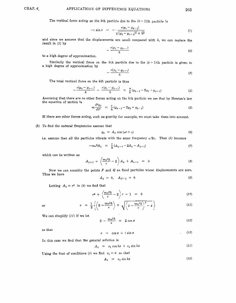
CHAP. 61 APPLICATIONS O F DIFFERENCE EQUATIONS
The vertical force acting on the kth particle due to the ( k - 11th
203
particle is
(1
and since we assume that the displacements are small compared with h, we can replace the result in ( I ) by
T(Yk - Yk-1) - h
to a high degree of approximation.
a high degree of approximation by Similarly the vertical force on the kth particle due to the ( k + 1)th particle is given
I_ r(Yk - Yk i 1)
h
The total vertical force on the kth particle is thus
t o
(3)
Assuming that there are no other forces acting on the kth particle we see that by Newton's law the equation of motion is
d2?-!k r dt2 = k ( Y k - 1 - 2Yk f Y k i 1) (5 )
If there are other forces acting, such as gravity for example, we must take them into account.
( b ) To find the natural frequencies assume that
Yk = Ak COS (Ot -I- CY) ( 6 )
i.e. assume that all the particles vibrate with the same frequency d 2 r . Then (5) becomes
Now we can consider the points P and Q as fixed particles whose displacements are zero. Thus we have
A0 0, AN+l = 0 ( 9 )
Letting Ak = ~k in (8) we find that
r 2 + (E+)Y+l = 0 (1 0 )
or
We can simplify (11) if we let mw2h - 2 -- - 2cose
7
so that r = cose I i sine . (13)
In this case we find that the general solution is
Ak = c1 coske + c2 sin ke
Using the first of conditions (9) we find c1 = 0 so that A k = C2 sinks

204 APPLICATIONS O F DIFFERENCE EQUATIONS [CHAP. 6
From the second of conditions (9) we must have
or since c2 # 0,
Thus (12) yields
f rom which
Denoting the N different values of w9 corresponding to n = 1,2,3, . . ., N by w1,02 ,w3, . . ., WN i t then follows tha t
n = 1 , 2 , ..., N (20) w, = f i s i n m n7r
Thus the natural frequencies a r e n r
f, = '6 2Ti sin- 2(LV +- 1) n = 1 , 2 , . . .,N
6.2. Find the displacement of the kth particle of the string in Problem 6.1.
i.e. the n th mode of vibration. the kth particle is given by
Let us consider the particular mode of vibration in which the frequency corresponds to w,, In this case we see from Problem 6.1 tha t the displacement of
Yk,n = A k , n (Writ + an) (1 )
(2) nl; c , sin - N + 1 where Ak,n
the additional subscript n being used for W, a and c to emphasize tha t the result is t rue for the nth mode of vibration.
Now since the difference equation is linear, sums of solutions a re also solutions so that we have for the general displacement of the kth particle
(3) nki; N
yk = 2 c, sin - cos (ant + a,) n=t N + l
Since this satisfies the boundary conditions at the ends of the string, i.e. yo = 0, Y N + ~ = 0, represents the required displacement.
of the N particles at the time t = 0.
it
The 2N constants c,, a,, n = 1, , , ., N , can be found if we specify the positions and velocities
6.3. Find the natural frequencies of the string of Problems 6.1 and 6.2 if the number of particles N becomes infinite while the total mass M and length L of the string re- main constant.
The total mass M and length L of the string a re given by
= Nm, L = (Ar+ ~ ) J L
Then the natural frequencies a re given by
or n7r f, = -L sin
2 s

CHAP. 61 APPLICATIONS O F DIFFERENCE EQUATIONS 205
Now for any particular value of n we have
[by using for example the fact that for small angles 8, sine is approximately equal to el. the required natural frequencies are given by
Thus
( 4 ) f = - L :& n=1 ,2 , ...
If we let p denote the density in this case, then
( 5 ) - _ : - p or M = ~ L
and (4 ) becomes
n=1,2 , ...
APPLICATIONS TO ELECTRICAL NETWORKS 6.4. An electrical network has the form shown in Fig. 6-4 where RI, RZ and R are given
constant resistances and V is the voltage supplied by a generator. (a) Use Kirch- hoff's laws to expess the relationship among the various currents. (b ) By solving the equations obtained in (a) find an expression for the current in any of the loops.
Fig. 6-4
(a) For the first loop, ZlRl + (ZI - 2 2 ) R z - V = 0
For the kth loop, + ( I k - I k + l ) R 2 - ( I k - l - I k ) R 2 = 0
For the ( N + 1)th loop, I N t l R l - ( z N - z N t 1 ) R 2 = 0
( b ) Equation (a) can be written as
Letting I k = r k in ( 4 ) it can be written as

206 APPLICATIONS O F DIFFERENCE EQUATIONS
Then the general solution of ( 4 ) is
I!, = clr: + c2rt
where
From ( I ) ,
From (3),
Now if we put k = 2 and k = N in (6) we have
I, = clr : -I- c2ri
I N = clr: + c2r:
from which z2rf - zNri rIrf - r,"rT '
INrT - Z2ry
ryr: - r i r r c1 = c2 =
so tha t
where r l , r2 a r e given in (7) and I,, Z, are given by (10) and (11) .
[CHAP. 6
APPLICATIONS TO BEAMS 6.5. IZI Derive the equation of three moments
( 4 ) on page 200.
Assume tha t the spacing between sup- ports is h and consider three successive sup- ports as shown in Fig. 6-5. Choosing origin 0 at the center support and letting x be the distance from this origin we find t h a t the bending moment a t x is given by
h 9: h -I
M"
Fig. 6-5
M , + (M,- M,-.l) -h 5 x 5 0
0 5 x 5 h M , + (M,+l-M,) ; M ( x ) =
where M,-l, M,,, M,+ a r e the bending moments at the (n - l ) th , nth and (n + 1)th supports.
Now we know from the theory of beams tha t the curve of deflection of a beam is y(x) where
YZy" = M(x) (2)
and YZ, called the flexural r ig id i ty of the beam, is assumed to be constant, modulus of elasticity and I is the moment of inertia about a n axis through the centroid.
Here Y is Young's
Integrating (2) using ( 1 ) we find
X2
X2
M,x + ( M n - M n - l ) c + ~1 -h S x 5 0
0 s x 5 h (8
M,x + ( M , + 1 - M n ) c + c2 r YZy' =
Now since y' must be continuous a t x = 0, i t follows tha t c1 = c2 = c.

CHAP. 61 APPLICATIONS O F DIFFERENCE EQUATIONS
Integrating (3) we have similarly
Since the deflection g is zero at x = -h, 0, h we find froni ( 4 )
Addition of these equations leads to the result
as required. M,-I + 4 M , + M n + l = 0
207
(7)
6.6. Suppose that the beam of page 200 is of infinite extent on the right and that a t the distance h to the left of the first support there is a load W which acts on the beam [see Fig. 6-61. Prove that the bending moment at the nth support is given by
Mn = (-I),+' Wh(2 - $3 )"
Fig. 6-6
The bending moment at the distance h to the left of the first support is given by
M , = - W h (1 1 Also at infinity the bending moment should be zero so that
lim M , = 0 n - + m
Now from the difference equation M,-1 + 4 M , + Mn+l = 0
we have on making the substitution M , = r n
r n - 1 + 4 r , + m + l = 0 o r r2+ 4 r + 1 = 0
i.e.
Then the general solution of (3) is
M , = ~ , ( - 2 + fl)" + c2(-2 - fi )"
(4)
Now since -2 + fi is a number between -1 and 0 while -2 - fi is approximately -3.732, i t fol- lows tha t condition (2) will be satisfied if and only if c2 = 0. Then the solution ( 5 ) becomes
M , = e l ( -2 + fi), ( 6 )
Also from (1) we have c1 = -Wh so tha t
M , = - W h ( - 2 + f i ) ' L = ( - l )n+lWh(2 - 'v6) ' (7)

208 APPLICATIONS O F DIFFERENCE EQUATIONS [CHAP. 6
APPLICATIONS TO COLLISIONS 6.7. Two billiard balls of equal mass m lie on a billiards table with their line of centers
perpendicular to two sides of the table. One of the balls is hit so that it travels with constant speed S to the other ball. Set up equations for the speeds of the balls before the kth impact occurs assuming that the table is smooth and the sides are perfectly elastic.
Denote by Uk and V k the speeds of the balls before the kth impact occurs. Then assuming tha t u k refers to the ball which is hi t initially we have
u1 = s, v1 = 0 (1 )
Since the sides a r e perfectly elastic, the speeds of the balls af ter the kth impact a r e U k t 1 and Vk+l respectively. Then the total momentum before and af ter the kth impact a re given by m u k + mVk and m u k + - mVk+ respectively. Thus by the conservation of momentum we have
mUk + mvk = mUk+l - mVk+l
or Uk f V k = Uk+l - Vk+l (2)
Uk+l f Vk+l = - E ( U k - V k ) (3)
In addition we have by Newton’s collision rule
where E is the coefficient of restitution between the two billiard balls.
The required equations a re given by (2) and (3) which are to be solved subject to the condi- tions (1).
6.8. Determine the speeds of the balls of Problem 6.7 before the kth impact. Wri t ing the equations (2) and (3) of Problem 6.7 in terms of the shifting operator E we obtain
(E - 1 ) u k - (E 1)Vk = O (1 )
( E f E ) U k + ( E - E ) V k = 0 (2)
( E 2 + e ) U k = 0 (3)
Then operating on (1) with E - E , on (2) with E + 1 and adding we obtain
Letting Uk = r k , (3) yields r 2 + , = 0, r = & i f i = fie..i/2
so t h a t the general solution of (3) i s
( 4 ) Tk Uk = ,k/2(AerkI/2 + Be-rkil2) = &/2 c1 cos- + c2 sin - ( 2
By eliminating Vk+l between equations (2) and (3) of Problem 6.7 we find
( E f 1 ) V k = 2Uk+l + ( E - 1 ) U k (5 )
Then using ( 4 )
(6) ak vk = E + 1 [ { ( e - 1)c2 - 2~ cl) sin - 2 + { ( e - 1)cl + 2 6 c2> cos -
From conditions (1) of Problem 6.7 we have / \
fi (cl cos 2 ?r + c2 sin - ;) = s (7)
so t h a t s
c2 = - fi ( E - 1)s
c1 = - 2 E ( 9 )

CHAP. 61 APPLICATIONS O F DIFFERENCE EQUATIONS 209
Using these in (4 ) and (6) we obtain the required results
APPLICATIONS TO PROBABILITY 6.9. A and B play a game. In each step of the game A can win a penny from B with
probability p while B can win a penny from A with probability q, where p and q are positive constants such that p + q = 1. We assume that no tie can occur. Sup- pose that the game is started with A and B having a and b pennies respectively, the total being a + b = N , and that the game ends when one o r the other has M pennies. Formulate (a) a difference equation and ( b ) boundary conditions for the probability that A wins the game.
Let u k be the probability tha t A wins the game when he has k pennies. one of the following two mutually exclusive events occurs:
Now A will win if
1. On the next step A wins a penny and then wins the game.
2. On the next step A loses a penny and then wins the game.
The probability of the first event occurring is given by
p u k + 1 (1 )
since if A wins on the next step [for which the probability is p ] he has k + 1 pennies and can then win the game with probability u k + l .
Similarly the probability of the second event occurring is given by
q u k - l (2)
since if A loses on the next step [for which the probability is q] he has k - 1 pennies and can then win the game with probability Uk-1 .
It follows t h a t the probability of A winning the game is the sum of the probabilities (1) and (2 ) , i.e.
u k = I ) u k + l + qZLk-1 (3)
To determine boundary conditions for uk we note tha t A wins the game when he has M pennies, i.e.
Similarly A loses the game when B has M pennies and thus A has N - M pennies, i.e.
uM = 1 ( 4 )
uN-M = 0 ( 5 )
6.10. Obtain the probability that A wins the game of Problem 6.9 if (a) p i q, ( b ) p = q = 4. We must solve the difference equation ( 3 ) of Problem 6.9 subject t o the conditions ( 4 ) and ( 5 ) .
To do this we proceed according to the usual methods of Chapter 5 by letting u k = y k in equation (8) of Problem 6.9. Then we obtain
p r z - - . + q = 0 (1)
( 2 )
from which 1kd- - - 1 k d 1 - 4 p + 4 p 2 - - 1 2 (1-2P) = 1, q / p
2 P 213 2P r =
( a ) If p # q, the roots of (1 ) a r e 1 and q l p so tha t
u k = c1 C2(q/p)k

210 APPLICATIONS OF DIFFERENCE EQUATIONS
Using the condition ( 4 ) of Problem 6.9, i.e. uM = 1, we have
1 = c1 + c z ( q / p ) M
Similarly using condition (5) of Problem 6.9, i.e. u ~ - ~ = 0, we have
0 = c1 + c z ( d f 3 ) N - M
Then solving ( 4 ) and (5) simultaneously we obtain
and so from (3) we have
Since A starts with k = a pennies, the probability that he will win the game is
while the probability that he loses the game is
[CHAP. G
(b ) If p = q = 8, the roots of (1) are 1, 1, i.e. they are repeated. In this case the solution of equation (3) of Problem 6.9 is
Uk = c3 + c4k (10)
Then using uM = 1, u ~ - ~ = 0, we obtain
~3 + c4M = 1, CS + c ~ ( N -M) = 0
i.e.
Substituting in (1 0)
1 - - M - N cs = ___
c 4 - 2 M - N 2 M - N '
M - N + k 2 M - N u k =
Thus the probability that A wins the game is
M - N + a 2 M - N u, =
while the probability that he loses the game is M - a 1-u, = ~ 2 M - N
6.11. Suppose that in Problem 6.9 the game is won when either A or B wins all the money, i.e. M = N . Find the probability of A being "ruined", i.e. losing all his money if (a) P f 4, ( b ) p = Q = 1/2.
(a) Putting M = N in equation (9) of Problem 6.10 we find for the probability of A being ruined
( b ) Putting M = N in equation (14) of Problem 6.10 we find for the probability of A being ruined
(2) 6
a f b N - a - - - 1-u, = - N

211 CHAP. 61 APPLICATIONS OF DIFFERENCE EQUATIONS
The case where p = q = 1/2 is sometimes called a “fair game” since A and B then have equal chances of getting a point at each step. From (2 ) we note that even in a fair game the chance of A being ruined is proportional to the initial capital of B. I t follows as a consequence that if B has many more pennies than A initially then A has a very great chance of being ruined.
This is illustrated by events which take place a t many gambling casinos where a person is competing in a game [which often is not even fair] against an “infinitely rich” adversary.
6.12. A and B play a game. A needs k points in order to win the game while B needs m points to win. If the probability of A getting one point is p while the probability of B getting one point is q, where p and q are positive constants such that p + q = 1, find the probability that A wins the game.
be realized if one of the following two possible mutually exclusive events occurs: Let u k , m denote the probability that A wins the game. The event that A wins the game can
1. A wins the next point and then wins the game.
2. A loses the next point and then wins the game.
The probability of the first event occurring is given by
PUk-- l ,m (1 1 since if A wins the next point [for which the probability is p ] he needs only k - 1 points to win the game [for which the probability is ~ l ~ - ~ , ~ ] .
Similarly the probability of the second event occurring is
qUk,m--l (2)
since if A loses the next point [for which the probability is q] he still needs k points to win the game while B needs only m- 1 points to win [for which the probability is U k , m - l ] .
It follows that the probability of A winning the game is the sum of the probabilities ( 1 ) and (a), i.e.
Uk,m = Puk--l,m + qUk,m--l (8)
To determine boundary conditions fo r Uk, , , we note that if k = 0 while m > 0, i.e. if A needs no more points to win, then he has already won. Thus
ug,m = 1 m > 0 ( 4 )
u k , o = 0 k > 0 ( 5 )
Also if k > 0 while m = 0, then B has already won so that
The solution of the difference equation (8) subject to conditions ( 4 ) and (5 ) has already been found [see Problems 5.53 and 5.54, page 1861 and the result is
FIBONACCI NUMBERS 6.13. Prove that the kth Fibonacci number is given by
We must solve the difference equation
F k = Fk-1 + Fk--2
subject to the conditions F” = 0, F1 = 1

212 APPLICATIONS O F DIFFERENCE EQUATIONS
Letting F k = rk in (1) we obtain the auxiliary equation
Then the general solution is
From the conditions (2) we find
c ,+c , = 0, ( l + f i ) C ~ + ( l - f i ) c , = 2
6’ fi 1 c2 = -- 1 Solving (5) we find
c1 = -
and so from ( 4 ) we have F k = L[(T)k 1 + f i - (!5.d!)k]
f i L
[CHAP. 6
F k + l = l + f i 2 - 6.14. Provethat lim Fk
k-tco
We have using Problem 6.13
Then since I (1 - fi )/(1+ fi ) I < 1 we have
This limit, which is equal to 1.618033988.. . , is often called the golden mean. represent the ratio of the sides of a rectangle which is “most pleasing” t o the eye.
I t is supposed to
MISCELLANEOUS APPLICATIONS 6.15. Evaluate the integral
do = cos kd - cos ka
sk = cl: cose - cosa
Let a, b, c be arbitrary constants and consider
7 U[COS ( k + 1)e - cos ( k + 1)a] de
cos e - cos a a s k + l + bSk + C s k - 1 =
+ f b[cos ke - cos ka]
+i do
cos e - cos (Y
i7 c[cos ( k - 1)s - cos (k - l)a] de
cos e - cos a
[(a + c) cos e + b] cos ke + [(c - a) sin 81 sin ke de
cos e - cos a

CHAP. 61 APPLICATIONS O F DIFFERENCE EQUATIONS 213
If we now choose a, b and c so that
c = a, b = -2acosa
the last integral becomes
2a l r c o s k e de = 0 if k = 1,2,3, ... It thus follows that
Sk+i-2(COSCX)Sk+Sk-l = 0 k = l , 2 , 3 ,... (1 )
so = 0, s1 = P (2)
From the definition of S k we have
We must thus solve the difference equation ( I ) subject to the conditions (2).
According to the usual methods for solving difference equations we let S k = r k in (1) and obtain
r k + l - ~ ( C O S a ) r k + r k - 1 = 0 or TZ - 2(cosa)r + 1 = 0
so that 2 cosa -r- d4 cos2a - 4 - - cos a f i sin 2 r =
Then by de Moivre's theorem, r k = coska f i s i n k a
so that the general solution is S k = c1 cos ka + c2 sin ka
Using the conditions (2) we have c1 = 0, c1 cosa + c2 sincr = T
so that c.,, = &ina and thus
which is the required value of the integral.
6.16. Find the value of the determinant
b a O O O . . . 0 0 0 a b a O O ... 0 0 0 O a b a O ... 0 0 0
0 0 0 0 0 . . . a b a 0 0 0 0 0 ... O a b
..............................
Denote the value of the kth order determinant by Ak. Then by the elementary rules for evalu- ating determinants using the elements of the first row we have
Ak = bAk-1 - U'Ak-2 or Ak - bAk-1 + U'Ak-2 = 0 (1 1
Letting Ak = r k we obtain yk - b r k - 1 + a2yk-z = 0 o r r2 - br + = 0
from which b * d m
2 r =

214 APPLICATIONS O F DIFFERENCE EQUATIONS [CHAP. 6
It i s convenient to let ’
SO t h a t (2) becomes T = a cose * ai sine
Thus since vk = ak(cos ke * i sin ke) we can write the general solution as
Ak = Uk[C1 COS ke + C2 Sin ke] (5)
Now if k = 1, the determinant of order 1 has the value A , = b, while if k = 2, the deter- minant of order 2 has the value
Put t ing k = 2 in (5 ) we find t h a t Rz - bA1+ &A0 = 0
from which we see on putting A , = b, A2 = b2- a2 tha t A . = 1. It follows t h a t we can solve (I) subject to the conditions
A0 = 1, A1 = b . (6)
These values together with (5 ) lead to
(7) b - u cos 6 - cos 6
6, = 1, c2 = - - a sin e sin e
using (3) so tha t (5) becorn& ak sin (k + 1)e
Ak = ak [eoske + sine cOsel = sin 8
Using the fact tha t
we can write the value of the determinant in the form
e = cos-1(b/2a)
a k sin [ ( k + 1) cos-1 (b/2a)] sin [cos-1 (b/2a)] Ak = -
or 2&+1 sin [(k + 1) cos-1 ( b / 2 a ) ]
Ak = d z F T
(9 )
The above results hold f o r Ibl < 21~1. I n case jbl > 21al we must replace cos-1 by cosh-1.
F o r the case 161 = 21aj see Problem 6.97.
6.17. A man borrows an amount of money A . He is to pay back the loan in equal sums S to be paid periodically [such as every month, every 3 months, etc.]. This payment includes one part which is interest on the loan and the other part is used to reduce the principal which is outstanding. If the interest rate is i per payment period, (a) set up a difference equation for the principal Pk which is outstanding after the kth payment and ( b ) solve fo r Pk.
( a ) Since the principal outstanding af ter the kth payment is Pk, i t follows tha t the principal out- standing af ter the ( k + 1)st payment is Pk+,. Now this last principal to be paid is the principal outstanding from the kth payment plus the interest due on this payment for the period minus the sum S paid for this period. Thus
Pk+l = Pk + ipk - s (1 )
or P k + l - ( I + i ) P k = -s The outstanding principal when k = 0 is the total debt A so that we have
Po = A (2)

CHAP. 61 APPLICATIONS O F DIFFERENCE EQUATIONS 215
(a) Solving the difference equation ( 1 ) we find
P k = c(1 +i)k + S/i
and using condition (2) we find c = A - S/ i so that
6.18. In Problem 6.17 determine what sum S is to be paid back each period so as to pay back the debt in exactly n payments.
We must determine S so that P, = 0. From Problem 6.17 this is seen to be equivalent t o
or
A ( l + i ) n - S [ (1 + i)" - 1 ] = 0
S r 1
The process of paying back a debt according to (2) and Problem 6.17 is often called amortization. The factor
(3 ) - 1 - (1 + i ) p
i " q i -
is often called the amortization factor and is tabulated for various values of n and i. In terms of this we can write (2) as
6.19. Given the differential equation
Show that if y(xk) = yk, y'(xk) = y; = f ( x k , yk) then the differential equation is ap- proximated by the difference equation
Y k + l = Y k + hy; = Y k + h f ( x k J ' Y k )
where h = Ax = x,,, - xk.
corresponding values of y are y k and y k + l respectively From the differential equation we have on integrating from x = x k t o % k + l for which the
or
If we consider f ( x , y) to be approximately constant between xk and xk+ 1, ( 2 ) becomes
as required.

216 APPLICATIONS O F DIFFERENCE EQUATIONS [CHAP. 6
k
0
1 2
3
4
5
6.20. (a) Use the method of Problem 6.19, sometimes called the Euler method, to find the value of y corresponding to x = 0.5 for the differential equation 4
xk 2/k 76d = f(xk, yk) yk + 1 = Yk + h2/i
0 1.0000 1.0000 1.1000
0.1 1.1000 1.3000 1.2300
, 0.2 1.2300 1.6300 1.3930
0.3 1.3930 1.9930 1.5923
0.4 1.5923 2.3923 1.8315
0.5 1.8315
- dy = 2x + y, v(0) = 1 dx (b ) Compare the result obtained in (a) with the exact value. (a) We have for initial conditions xo = 0, yo = 1. Then by Problem 6.19 with k = O , l , 2, . . .
we find 2/1 = Yo $- hfb0,YO) 762 = ?dl + hLf(X1,Yl) Y3 = Y, + hf(X2,Yz) (1 1 etc.
We can use a convenient value for h, for example h = 0.1, and construct the table of Fig. 6-7 using equations (1) with f(Xk, yk) = 2xk + yk.
Fig. 6-7
From the table we can see t h a t the value of y corresponding to x = 0.5 is
( b ) The differential equation can be written as
_ - dy y = 2x dx
1.8315.
(2)
a first order linear differential equation having integrating factor e ’ ( - I ) dZ = e-5. Multiplying by e-X we have
Thus on integrating,
e-xy = 2xe-Xdx = -2xe-5 - 2e-5 + c
y = -2x - 2 + cex (3)
y = 3e5- 2x - 2 ( 4 )
y = 3eo.5 - 2(0.5) - 2 = 3(1.6487) - 3 = 1.9461 (5 )
s or
Since Y = 1 when x = 0, we find c = 3. Thus the required solution is
Put t ing x = 0.5 we have for the required value of y
It is seen t h a t the result i n (a) is not too accurate since the percent error is about 64%. Better results can be obtained by using smaller values of h for example h = 0.05 [see Problem 6.1011.
This method, also called the step by step method, is important because of its simplicity and also theoretical value. There a re of course many methods which provide greater accuracy. One of these which is a modification of the Euler method presented here is given in Problems 6.21 and 6.22. Other methods a re given in the supplementary problems.

217 CHAP. 61 APPLICATIONS OF DIFFERENCE EQUATIONS
6.21. Given the differential equation of Problem 6.19 show that a better approximation is given by the difference equation
Yk+l = Y k + W ( Y , ' + Y;+J Using equation ( 2 ) of Problem 6.19 we have
Instead of assuming t h a t f(x, y) is practically constant over the range from $k to Xk+ trapezoidal rule to approximate the integral in (1).
we use the We thus obtain
6.22. Use the method of Problem 6.21, sometimes called the modified Euler method, to work Problem 6.20.
In order to start the procedure using Problem 6.21 we must first find a n approximate value of y corresponding to x = 0.1, assuming t h a t we choose h = 0.1 as in Problem 6.20. F o r this pur- pose we use the ordinary Euler method of Problem 6.20 and find
The initial values of x and y a re xo = 0, yo = 1 and a r e entered in the table of Fig. 6-7.
Yl = Y(O.1) = Yo + hf(xo,YrJ) = Yo + hYd
= 1.0000 + 0.1(1.0000)
= 1.1000
This is entered in the table of Fig. 6-8 under Approximation I.
5 0.5 1.9247 2.9247 1.9471 2.9471 1.9482 2.9482 1.9483
Fig. 6-8
This is entered in the table of Fig. 6-8 under Approximation I.
I I I I I I I I
Fig. 6-8
From the differential equation we now find
YI = f ( % Y l ) = 2x1 + Yl = 2(0.1) + 1.1000
= 1.3000
which i s also entered under Approximation I in Fig. 6-8. From the modified Euler formula of Problem 6.21 we have on putting k 0
Y1 = =
= 1.1150
Yo -i- &h(ldA+- Y;) 1,0000 3- +(0.1)(1.0000 + 1.3000)
This better approximation to yl is entered in the table of Fig. 6-8 under Approximation 11.

218 APPLICATIONS O F DIFFERENCE EQUATIONS [CHAP. 6
Repeating the process we then find
Y; = f(X1,Yl) = 2x1 + Y 1 = 2(0.1) + 1.1150 = 1.3150
and so Approximation I11 for y, i s given by
which yields
We then find
Y, = Yo + -p(Yi+Y;) =
= 1.1153
1,0000 + ~(0.1)(1.0000 + 1.3150)
I/; = f ( X 1 , Y l ) = 2x1 + Y l
= 2(0.1) i- 1.1158 = 1.3158
?dl = =
= 1.1158
I40 + $h(Yi+ YI) 1.0000 + +(0.1)(1.0000 + 1.3158)
Since this gives the same value as tha t obtained above for y1 the desired accuracy to four decimal places i s achieved.
We now proceed in the same manner to find y(0.2) = y8. Using the value y1 = 1.1158 cor- responding to x1 = 0.1 we have for Approximation I
Y2 = Y1 + hf(x,,ld,) = Y l + hYf = 1.1158 + O.l(l.3158) = 1.2474
and Y; = f(X2,Y2) = 2x2 + I42
= 2(0.2) + 1.2474
= 1.6474
By continuing the process over and over again we finally obtain the required value y5 = ~ ( 0 . 5 ) = 1.9483 as indicated in the table. This compares favorably with the exact value 1.9461 and is accurate to two decimal places.
It will be noticed t h a t in the modified Euler method the equation
Y k t l = Yk + &h(YL+?dLtl) is used to “predict” the value of yk+1. The differential equation
Yk = f(xk,Yk) is used to “correct” the value of ykfl . dictor-corrector” method. example Problem 6.105.
Because of this we often refer to the method as a “pre- See for Many such methods a r e available which yield better accuracy.
6.23. Show how the boundary-value problem
U(x,O) = 1, U(x , l ) = 0, U(0, y) = 0, U(1, y) = 0 ’ can be approximated by a difference equation.
It is convenient to approximate the derivatives by using central differences. If we let 8, and Ex denote the central difference operator and shifting operator with respect to x, then the partial derivative operator with respect to x is given by
El/Z - E-l/2 a 8, -
ax X z - - - _
h h
Thus by squaring the operators and operating on
D, =
where the symbol - denotes “corresponds to”. U we have

CHAP. 61 APPLICATIONS O F DIFFERENCE EQUATIONS 219
1 - ( E x - 2 + E L ~ ) U ( S , y) hz =
1 = h2 [ U ( x + h, Y) - 2Wx, Y) + U ( x - h, Y)]
Similarly using operators with respect to y we have
It follows by addition t h a t
Thus the equation
is replaced by u (2 + h, Y) + U ( x - h, y) + U ( x , y + h) + V ( x , y - h) - 4U(x, y) = 0
or U ( x , Y) = A[U(x + h, Y) + U ( x - h, Y) + U(X, y + h) + U ( x , y - h)] which is the required difference equation,
(1 1
The boundary conditions associated with this difference equation a re left the same.
6.24. Show how to obtain an approximate solution to the boundary-value problem of Problem 6.23.
We must find U ( X , ? J ) at all points inside the square 0 5 x 5 1, 0 5 y 5 1.
The result is often called a gr id or mesh.
Using a suitable value of N and h such tha t hrh = 1, we subdivide the square into smaller squares of sides h = 1/N as in Fig. 6-9. Instead of finding U ( X , y) at all points inside the square we find the values of U ( x , y) a t the points of the grid such as A , B , . . . in Fig. 6-9. To accomplish this we make use of the difference equation ( 1 ) of Problem 6.23 which is, as we have seen, an approximation to the partial differential equation. By referring to Fig. 6-10, which represents a n enlargement of a par t of Fig. 6-9, we see tha t this difference
states t h a t the value of U at P is the arithmetic mean of the values at the neighboring points A , B, C and D. By using this difference equation together with the values of U on the boundary of the square as shown in Fig. 6-9, we can obtain approximate values of U at all points in the grid.
C(0, y) = 0
-
Y I I L'ix. 1) = 0 B
Fig. 6-9 Fig. 6-10

220
Trial Number
1
APPLICATIONS O F DIFFERENCE EQUATIONS
Ul u, u3 u4
0 0 0 0
In order to illustrate the procedure we shall use the grid of Fig. 6-11 in which we have chosen for the purposes of simplification h = 1/3. In this case there are four points in the grid denoted by 1 , 2 , 3 , 4 of Fig. 6-11. We wish to find the values of U a t these points denoted by Ul, U2, U3, U4 respectively.
By applying equation (1) we see that U1, U2, U3, U4 must satisfy the equations
u=o
u1 = & ( O + O + U 2 + U 3 )
u3 = Q ( O + U 1 + U 4 + 1 ) (2) U = l U, = & ( U l + 0 4 0 + U 4 )
U, = $ ( U 3 + U 2 + O + l ) Fig. 6-11
[CHAP. 6
u = o
The first equation for example is obtained by realizing that U1, i.e. the value of U at point 1, is the arithmetic mean of the values of U at the neighboring points, i.e. O,O, U,, U3 the zeros being the values of U at points on the boundary of the square.
The values U1, U,, U3 and U4 can be found by solving simultaneously the above system of equations. For a grid with a large number of subdivisions this procedure is often less desirable than a method called the method of iteration which can take advantage of machine calculators.
The simplest is to take U1 = 0, U , = 0, U3 = 0, U, = 0. We refer to this as Trial Number 1 or the first trial as re- corded in Fig, 6-12.
Using the values of U1, U2, U3, U4 from the Trial 1 in equation (2) we then calculate the new values
In this method of iteration we first assume a trial set of solutions.
U1 = 0, UZ = 0, U3 = 0.2500, U4 = 0.2500
These are entered in Fig. 6-12 for Trial 2.
Fig. 6-12
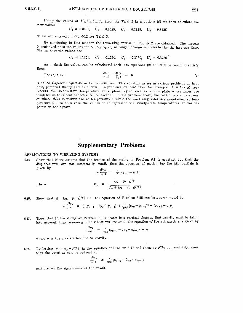
221 CHAP. 61 APPLICATIONS O F DIFFERENCE EQUATIONS
Using the values OP Ul, U,, U3, U , from the Trial 2 in equations (2) we then calculate the new values
U ; = 0,0625, Ug = 0.0625, U3 = 0.3125, U, = 0.3125
These a r e entered in Fig. 6-12 for Trial 3.
The process is continued until the values foi. U,, U,, Us, U4 no longer change as indicated by the last two lines. We see t h a t the values a r e
By continuing in this manner the remaining entries in Fig. 6-12 a r e obtained.
U1 0.1250, U , = 0.1250, U 3 = 0.3750, U4 = 0.3750
As a check the values can be substituted back into equations (2) and will be found to satisfy them.
The equation
is called Laplace’s equation in two dimensions. This equation arises in various problems on heat flow, potential theory and fluid flow. U = U(x,y) rep- resents the steady-state temperature in a plane region such as a thin plate whose faces a re insulated so tha t heat cannot enter o r escape. In the problem above, the region is a square, one of whose sides is maintained at temperature 1 while the remaining sides a r e maintained at tem- perature 0. In such case the values of U represent the steady-state temperatures at various points in the square.
In problems on heat flow for example,
Supplementary Problems APPLICATIONS TO VIBRATING SYSTEMS 6.25. Show t h a t if we assume that the tension of the s t r ing in Problem 6.1 is constant but tha t the
displacements a re not necessarily small, then the equation of motion for the kth particle is given by
m- - dtz
where
6.26. Show t h a t if l(yk - ~lc-l)/IzI < 1
m- = - ( ( ~ k - : - 2 ~ k + ~ k + 1 ) + - - I - [ ( ~ k - ~ y i i - : ) ~ - ( ~ k t i - ~ k ) ~ I
the equation of Problem 6.25 can be approximated by
d2yk r dt2 h 2h3
6.27. Show t h a t if the s t r ing of Problem 6.1 vibrates in a vertical plane so tha t gravity must be taken into account, then assuming t h a t vibrations a re small the equation of the kth particle is given by
where g is the acceleration due to gravity.
6.28. By letting ifk = u,+F(lc) in the equation of Problem 6.27 and choosing F ( k ) appropriately, show tha t the equation can be reduced to
and discuss the significance of the result.

222 APPLICATIONS O F DIFFERENCE EQUATIONS [CHAP. 6
6.29. Suppose tha t the string of Problem 6.27 fixed at points P and Q [see Fig. 6-11 is left to hang vertically under the influence of gravity. Show tha t the displacement yk of the kth particle is given by
yk = -- mg 27h X k ( L - Xk) k = 1,2, . . . , N
where xk = kh i s the distance of the kth particle from P.
6.30. Suppose t h a t in the string of Problem 6.1 the number of particles N becomes infinite, in such a way t h a t the total mass and length a r e constant. Show tha t the difference equation in this limiting case becomes the wave equation
where T is the tension and p is the density [mass per unit length] of the string, both assumed constant.
6.31. What does the equation of Problem 6.30 become if the vibration takes place in a vertical plane and gravity is taken into account?
6.32. Suppose t h a t in Problem 6.1 the tension in the string is not constant but t h a t in the portion of the s t r ing immediately to the r ight of particle k the tension is r k . Show tha t the equation of motion of the kth particle is
d2yk _ _ 1 m- - h A ( T k - l & k - 1 ) d t2
and write corresponding boundary conditions.
(a) By letting yk = A!, cos w t in the equation of Problem 6.32 show t h a t we obtain the Sturm- Liouville difference equation
A(Tk- iAz4k- i ) + W d h A k = 0
( b ) Discuss the theory of the solutions of this equation from the viewpoint of eigenvalues and eigenfunctions a s presented in Chapter 5.
(c) Illustrate the results of this theory by considering the special case where the tension is constant.
6.33. Suppose t h a t at time t = 0 the position and velocity of the kth particle of Problem 6.1 a re given by y k ( 0 ) and &(O). Show tha t the position of the kth particle at any time t > 0 is given by
nkr N nkr N
yk = nzl c, sin K1 cos (ant + a,) = 2 (a, cos w,t + b, sin writ) sin - n=l N + l
where a,, b, or c, and are determined from
- b, = -en sin an
6.34. (a) Show that, if the ( N i . 1)th mass of the string of Problem 6.1 is free while the first mass is fixed, then the frequency of the lowest mode of vibration is
( b ) What a r e the frequencies of the higher modes of vibration? [Hint. If the force on the ( N + 1)th mass is zero then yx = YN+~.]
6.35. (a) Give a physical interpretation of the boundary conditions C U O Y O + alY1 = 0, axY.v aAT+l?dN+l = 0 in Problem 6.1.
( b ) Obtain the natural frequencies of the system for this case.

223 CHAP. 61 APPLICATIONS O F DIFFERENCE EQUATIONS
6.36.
6.37.
6.38.
6.39.
6.40.
6.41.
6.42.
An axis carries N equally spaced discs which a re capable of torsional vibrations relative to each other [see Fig. 6-13]. If we denote by ek the angular displacement of the kth disc relative to the first disc show tha t
d2ek I - dt2 = " ( ' k t l - 2 8 k + @k--1)
where Z is the constant moment of inertia of each disc about the axis and u is the torsion constant.
Fig. 6-13
(a,) Using appropriate boundary conditions obtain the natural frequencies for the system of Problem 6.36.
( b ) Explain how you would find the motion f o r the kth disc by knowing the s ta te of the system at time t = 0.
(c) Compare with results for the vibrating system of Problem 6.1.
Work Problem 6.37 if the first disc is fixed while the las t is free.
A frictionless horizontal table AB has on it N identical objects of mass m connected by identical springs having spring constant K as indicated in Fig. 6-14. The system is set into vibration by moving one or more masses along the table and then releasing them.
k m k m 0 . 0 . +-)qyp+
A B Fig. 6-14
(a) Letting % k denote the displacement of the kth object, set up a difference equation. ( b ) Find the natural frequencies of the system. (c) Describe the analogies with the vibrating s t r ing of Problem' 6.1.
Suppose that the s t r ing of Problem 6.1 with the attached particles is rotated about the axis with uniform angular speed a. (a) Show t h a t if yk is the displacement of the kth particle from the axis, then
y k t l - 2 (1 -3) Y k 4- y k - 1 = 0
( b ) Show t h a t the critical speeds in case m i P h f 4 r < 1 are given by - $2, = nr - sin - mh 2(N + 1)
n = l , 2 , . . . and discuss the physical significance of these.
Discuss the limiting case of Problem 6.40 if N + 5) in such a way that the total mass and length remain finite.
Explain how you would find a solution to the partial differential equation in Problem 6.30 subject to appropriate boundary conditions by applying a limiting procedure to the results obtained in Problem 6.2.

224 APPLICATIONS O F DIFFERENCE EQUATIONS [CHAP. 6
APPLICATIONS TO ELECTRICAL NETWQRKS 6.43. An electrical network consist,s of N loops with capacitors having constant capacitance C1, C2
in each loop as indicated in Fig. 6-15. An alternating voltage given by V N = K sin at where K and o a r e constants is applied across A$,. If i t is required tha t the voltage across A& be v, = 0, show tha t the voltage Vk across AkBk is given by
sinh ,uk sinh fiN Vk = K -- sin at
Fig. 6-15
Work Problem 6.43 if the capacitors C1 and C, a r e replaced by inductors with constant inductance 6.44. Ll, Lz.
6.45.
6.46.
Work Problem 6.43 if the capacitors C, a re replaced by resistors having constant resistance Rl.
Can Problem 6.43 be worked if i t is required t h a t the voltage across A$, be Vo > O ? Explain.
APPLICATIONS TO BEAMS 6.47. Suppose that in Problem 6.6 the beam is of finite length NF,.
at the n t h support is given by Show tha t the bending moment
Tntl- -N I n t l - - N r2
M , = -Wh[ ~ 1 - N - 1 -1 1 1-N
where rl = -2 + fi, r2 = -2 - g3. 6.48. Show t h a t as N + m the result in Problem 6.47 reduces to tha t of Problem 6.6.
6.49. In Fig. 6-16 A B represents a continuous uniform beam on which there is a triangular load dis- tribution where the total load on the beam is W. Suppose tha t the beam is simply supported at the W + 1 points Po,P,, . . .,P, at distances h apart. (a) Show tha t the three moment equation can be written as WIL
N2 M k - 1 + 4fi!f, + Ml,+l =
where the bending moments a t the ends A and B are zero, i.e. iM, = 0, M v = 0. the bending moment at the kth support is given by
( b ) Show that
Fig. 6-16
where
B
6.50. Does lim M k exist in Problem 6.49? Explain. N-+m

CHAP. 61 APPLICATIONS O F DIFFERENCE EQUATIONS 225
APPLICATIONS TO COLLISIONS 6.51. Show tha t the speeds of the balls in Problem 6.7 follow a periodic pattern and determine this
period.
6.52. ( a ) Work Problem 6.7 if the two masses a r e given by m, and m2 where ml f m2. (b) Determine the values of m,lm2 for which the speeds will be periodic and determine the periods in such cases. (c ) Discuss the motion for the case ml = 2m2.
6.53. A billiard ball is at res t on a horizontal frictionless billiards table which is assumed to have the shape of a square of side 1 and whose sides a r e assumed to be perfectly elastic. The ball is hit so t h a t i t travels with constant speed S and so tha t the direction in which it travels makes the angle e with the side. Determine the successive points a t which the ball hits the sides.
6.54. What additional complexities arise in Problem 6.53 if the billiard table has the shape of a rec- tangle? Explain.
APPLICATIONS TO PROBABILITY 6.55.
6.56.
6.57.
658.
Suppose that in Problem 6.9 we let Uk,m be the probability of A winning the game when he has k pennies while B has m pennies.
( a ) Show t h a t the difference equation and boundary conditions for U k , m a r e given by
U k , m = Puk+l,m-l + qUk-l ,mtl
~ M , N - M = 1, U N - M . M = 0
( b ) Solve the difference equation in ( a ) subject to the conditions and reconcile your results with those given in Problem 6.9. [Hint. See Problem 5.59, page 189.1
Suppose t h a t i n a single toss of a coin the probabilities of heads o r tails a r e given by p and q = 1 - p Let Uk,,$ denote the probability tha t exactly k heads will appear in 12
tosses of the coin. respectively.
( a ) Show tha t
where u k , 0 i: k = O k > O
This is called Bernoulli’s probability formula for repeated trials.
Suppose tha t A and B play a game a s in Problem 6.9 and that A star ts out with 10 pennies while B starts out with 90 pennies. ( a ) Show that if p = q = 1/2, i.e. the game is fa i r , then the probability tha t A will lose all of his money, i.e. A will be “ruined”, is 0.9. ( b ) Show tha t if p = 0.4, q = 0.6 then the probability that A will be “ruined” is 0.983. (c) Discuss the sig- nificance of the result in ( b ) if A represents a “gambler” and B represents the “bank” at a gambling casino. (d ) What is the significance of the result in ( b ) if A is the “bank” and B is the “gambler” ?
Suppose t h a t in Problem 6.9 p > q, i.e. the probability of A’s winning is greater than tha t of B. Show t h a t if B has much more capital than A then the probability of A escaping “ruin” if he starts out with capital a is approximately
1 - (alp)“
What is this probability if p = 0.6, q = 0.4 and ( a ) a = 5, ( b ) a = l o o ?

[CHAP. 6 226 APPLICATIONS O F DIFFERENCE EQUATIONS
6.59. Let Dk denote the expected duration of the game in Problem 6.9 when the capital of A is k.
( a ) Show t h a t D , satisfies the equation
Dk = p D k + I + q D k - 1 + 1 , DO = 0, D a + b = 0
k ( b ) Show t h a t if p # q , Dk = - - -
(c) Show t h a t if p = q = 112, Dk = k(a+b - k) and thus tha t if A and B start out with initial capitals a and b respectively the expected duration is ab.
6.60. Work Problems 6.9-6.11 in case a tie can occur a t any stage with constant probability B > 0 so t h a t p + q + E = 1.
THE FIBONACCI NUMBERS 6.61.
6.62.
6.63.
6.64.
6.65.
6.66.
6.67.
6.68.
6.69.
Let F , denote the kth Fibonacci number and let R k = FkIF,+l.
, R, = 0. 1 1 t Rk-1 Show t h a t Rk =
1 1
Show t h a t Rk =
1 1 +
l + -
* 1 + - 1 i.e. a continued fraction with k divisions.
Solve the difference equation of par t (a) in Problem 6.61 for Rk.
Show tha t lim Rk = 5-2 and thus obtain the limiting value of the infinite continued k - r 01 2
fraction in p a r t ( b ) of Problem 6.61.
If Fk denotes the kth Fibonacci number prove tha t
Fk+lFk,-I - F t = ( - l ) k k = 1 , 2 , 3 , . . .
Generalize Problem 6.63 by showing t h a t
Fkt ,nFk-m- F ; = ( - l )k+m-IF; k = m , m + l , m + 2 , . . .
A planted seed produces a flower with one seed a t the end of the first year and a flower with two seeds at the end of two years and each year thereafter. Assuming tha t each seed is planted as soon as i t is produced show t h a t the number of flowers at the end of k years is the Fibonacci number F k .
Find the number of flowers at the end of k years in Problem 6.65 if a planted seed produces a flower with four seeds at the end of the first year and a flower with ten seeds at the end of two years and each year thereafter.
Generalize Problems 6.65 and 6.66 by replacing ‘‘four seeds” and “ten seeds” by ‘ (a seeds” and “ b seeds” respectively. What restriction if any must there be on a and b ?
where F , is the kth Fibonacci number. - F k t 2 Find the sum of the series 2
k = O F k i l F k t 3
Show that
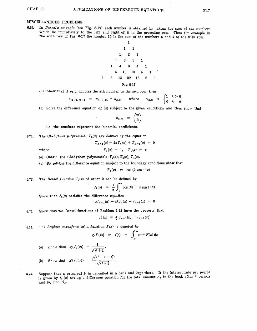
CHAP. 61 APPLICATIONS OF DIFFERENCE EQUATIONS 227
MISCELLANEOUS PROBLEMS 6.70. In Pascal's triangle [see Fig. 6-17] each number is obtained by taking the sum of the numbers
which lie immediately to the left and right of it in the preceding row. Thus for example in the sixth row of Fig. 6-17 the number 10 is the sum of the numbers 6 and 4 of the fifth row.
1 1 1
1 2 1 1 3 3 1
1 4 6 4 1 1 6 1 0 1 0 6 1
1 6 16 20 16 6 1
Fig. 6-17
(a) Show that if U,k,m denotes the kth number in the mth row, then 1 k > O 0 k = O U k t l , m + l = u k + l , m + Uk,m where uk,O =
( b ) Solve the difference equation of ( a ) subject to the given conditions and thus show that
uk,m = (3 i.e. the numbers represent the binomial coefficients.
6.71. The Chebyshev polynomials Tk(x) are defined by the equation
Tk+I(x) - 2%Tk(X) f Tk- i ($) = 0 where To(%) = 1, TI(%) = x
( a ) Obtain the Chebyshev polynomials T&), T3(x) , T&). ( b ) By solving the difference equation subject to the boundary conditions show that
T k (8) = COS (k COS-l X)
6.72. The Bessel funct ion Jk(X) of order k can be defined by
Show that Jk(x) satisfies the difference equation
d k + i ( Z ) - ZkJk(x) f Jk- i (X) = 0
6.73. Show that the Bessel functions of Problem 6.72 have the property that
JL(X) = &[Jk-l(X) - J k + l ( X ) ]
6.74. The Laplace transform of a function F(x ) is denoted by
dl{F(x)) = f ( 4 = [ O0e--ss F(x ) dx
( a ) Show that <{Jo(x)> = A @ T i '
6.75. Suppose that a principal P is deposited in a bank and kept there. If the interest rate per period is given by i, ( a ) set up a difference equation for the total amount A k in the bank after k periods and ( b ) find A k .

228
6.76.
6.77.
6.78.
6.79.
6.80.
6.81.
6.82.
6.83.
APPLICATIONS O F DIFFERENCE EQUATIONS [CHAP. 6
A man deposits a sum S in a bank a t equal periods. a difference equation for the amount A , in the bank after n periods and ( b ) show that
If the interest rate per period is i, (a) set up
(1+i)" - 1 = Ssqi An = S [ i ] Such a set of equal periodic psyments is called an annuity.
Work Problem 6.76 if the successive deposits are given by S, S + a, S + 2a, S f 3a, . . . . the significance of the cases (a ) a > 0, ( b ) a < 0.
Discuss
In a particular town the population increases a t a rate a% per year [as measured a t the end of each year] while there is a loss of p individuals per year. Show that the population after k years is given by
p , = ( P o - T ) ( l + & ) k + 9 . .
where Po is the initial population.
Does the result of Problem 6.78 hold if (a) a: < 0, p < 0, Interpret each of the cases.
( b ) a > 0, p < 0, (c) a < 0, /3 > O?
Let S k denote the sum of the kth powers of the n roots of the equation
p + all'n-l + a2rn-Z + . . . + a , = 0
(a) Show that S1 + al = 0, Sz + alSz + 2a2 = 0, . . ., S, + + + an-,S1 + nu, = 0
( b ) Show that if k > n Sk + a l S k - 1 + azSk-2 + * ' * + anSk-n = 0
Obtain the generating function for the sequence S k of Problem 6.80.
A box contains n identical slips of paper marked with the numbers 1, 2, . . ., n respectively. The slips are chosen at random from the box. We say that there is a coincidence if the number M is picked at the Mth drawing. Let u k denote the number of permutations of k numbers in which there are no coincidences. ( a ) Prove that the number of permutations in which there is 1 coin-
cidence is (:) uk-1. ( b ) Prove that the number of permutations in which there are m coincidences \ I
is (3 Uk-m where m = o , ~ , . . . ,k .
Prove that u, in Problem 6.82 satisfies the equation
By solving the difference equation in (a) prove that
Show that the probability of getting no coincidences in the drawing of the n slips from the box of Problem 6.82 is given by
+ - 1 1 - - - + ... 2! 3! n !
Show that for large values of n the probability in (c) is very nearly
1 - = 0.63212.. .
Discuss how large n must be taken in (d ) so that the probability differs from 1 - l / e by less than 0.01.

CHAP. 61 APPLICATIONS O F DIFFERENCE EQUATIONS
6.84.
6.85.
6.86.
6.87.
6.88.
6.89.
6.90.
6.91.
6.92.
An inefficient secretary puts n letters a t random into n differently addressed envelopes. that the probability of getting a t least one letter into its correct envelope is given by
Show
( - 1 ) n + l +- 1 1 1 1 - - + - - - + ... 2! 3 ! 4 ! n !
and thus show that for large n this probability is about l l e = 0.36787.. . . Can you explain from a qualitative point of view why this probability does not change much with an increase of n as for example from 100 to 200?
Find the probability that a t least two people present at a meeting will have their birth dates the same [although with different ages].
A group of players plays a game in which every time a player wins he gets ~, times the amount of his stake but if he loses he gets t o play again. Let u k denote the stake w%ch a player must make in the kth game so that he gets back not only all that he has lost previously but also a profit P . ( a ) Show that u k satisfies the sum equation
k
p=1 m u k = P + 2 up
( b ) Show that the sum equation of (a) can be written as the difference equation
(c) Using appropriate boundary conditions show that k
State some limitations of the “sure profit” deal in Problem 6.86 illustrating the results by taking m = 2.
A box contains slips of paper on which are written the numbers 1, 2, 3, . . ., n [compare Problem 6.821. Let ‘lLk,n denote the number of permutations [out of the total of n ! permutations] in which there is no coincidence in k given drawings.
The slips are drawn one at a time from the box a t random and are not replaced.
(a) Show that u k , m = u k - - l , m - uk--l,m--li Uk,o = k!
( b ) Show that the solution to the difference equation of part (a) is
(c) Show that the probability that there will be no coincidence in the k drawings is U k , m h ! .
( d ) Show that for k = m the probability obtained in (c) reduces to that obtained in Problem 6.82.
A and B play a game with a deck of n cards which are faced downwards. card. removed from the deck. and over again until there are no cards left, wins the game, otherwise B wins the game,
A asks B t o name a Then A shows B the card and all the cards above i t in the deck and all these cards are
A then asks B to name another card and the process is repeated over If B does not name any of the top cards then A
Find the probability that A wins the game.
If the deck of Problem 6.89 has 52 cards, determine whether the game is fair if B offers A 2 to 1 odds.
A sequence has its first two terms given by 0 and 1 respectively. obtained by taking the arithmetic mean of the previous two terms. of the sequence and ( b ) find the limit of the sequence.
Each of the later terms is ( a ) Find the general term
An urn has b blue marbles and r red marbles. each one is returned following the next marble taken. marble taken from the urn is blue if i t is known that the nth marble taken is blue.
Marbles are taken from the urn one at a time and Determine the probability that the kth

230 APPLICATIONS OF DIFFERENCE EQUATIONS [CHAP. 6
6.93.
6.94.
In the preceding problem what is the probability if nothing is known about the nth marble taken?
( a ) Show that the Stirling numbers of the second kind satisfy the equation
( b ) Use ( a ) to show that
and verify this for some special values of k and m.
6.95. There are three jugs which have wine in them. Half of the wine in the first jug is poured into the second jug. Then one-third of the wine in the second jug is poured into the third jug. Finally one-fifth of the wine in the third jug is poured back into the first jug. Show that after many repetitions of this process the first jug contains about one-fourth of the total amount of wine.
6.96. Generalize Problem 6.95.
6.97.
6.98.
6.99.
6.100.
6.101.
6.102.
6.103.
6.104.
6.105.‘
( a ) Show that Newton’s method [Problem 2.169, page 781 is equivalent to the difference equation
x, - - xg = a f (En)
f’(xn) ’ -
X n t 1 - ( b ) Can you find conditions under which lim x, exists? Justify your conclusions.
n+-
( a ) Prove that lim x, exists and is equal to fl. ( b ) Show how the result of (a) can be used to find fi t o six decimal places.
I t - m
9 Can you formulate a method for finding fi analogous to that of Problem 6.99.
Work Problem 6.20 by using h = 0.06 and discuss the accuracy.
( a ) Solve the differential equation - dy = x + y, y(0) = 1 dx
for y(0.6) using h = 0.1 by using the Euler method and compare with the exact value.
( b ) Work par t (a) using h = 0.05.
Work Problem 6.22 by using h = 0.05 and discuss the accuracy.
Given the differential equation - dy = x y q y(1) = 1 dx
( a ) Use the Euler method t o find ~ ( 1 . 5 ) and compare with the exact value.
( b ) Find y(1.5) using the modified Euler method.
(a) Obtain from the equation * = f(x, V ) the approximate “predictor” formula dx h
y k + l = yk-1 + -(Y;-1+4Y{+y{+1) 3
( b ) Explain how the result in ( a ) can be used to solve Problem 6.20 and compare the accuracy with the modified Euler method.

23 1 CHAP. 61 APPLICATIONS OF DIFFERENCE- EQUATIONS
6.106.
6.107.
6.108.
6.109.
6.110.
6.111.
6.112.
6.113.
6.114.
6.115.
6.116.
6.117.
6.118.
6.119.
(a) Explain how the method of Taylor series can be used to solve a differential equation. trate the method of (a) by working Problem 6.20. ferentiations y” = 1 + y’, y”’ = y”, . . . .
2 !
( b ) Illus- If y’ = x + y, then by successive dif-
Now use the Taylor series y(z) = y(a) + (z - &’(a) + [Hint.
*I (x - a)2y”(a) + . . . Work (a) Problem 6.102, ( b ) Problem 6.104 by the method of Taylor series,
Explain the advantages and disadvantages of (a) the Euler method, ( b ) the modified Euler method, (c) the Taylor series method for solving differential equations.
(a) Explain how the Euler method can be used to solve the second order differential equation
2 = f ( X , Y , $ )
( b ) Use the method of (a) t o solve
- d2y = x + y, y(0) = 1, y’(0) = 0 dx2
for y(0.5) and compare with the exact value.
Show how the differential equation of Problem 6.109(a) can be solved using the modified Euler method and illustrate by solving the differential equation of Problem 6.109(b).
Work Problem 6.109(b) by using the Taylor series method.
Explain how you would solve numerically a system of differential equations. Illustrate your procedure by finding the approximate value of x(0.5) and y(0.5) given the equations
and compare with the exact value.
Work Problem 6.24 by choosing a grid which is subdivided into 16 squares.
Explain how you could use the results of Problem 6.24 or 6.113 t o obtain the steady-state temperature in a square plate whose faces are insulated if three of its sides are maintained a t O°C while the fourth side is maintained a t 100OC.
Explain how you could use the results of Problem 6.24 or 6.113 t o obtain the steady-state tem- perature in a square plate if the respective sides are kept a t 2OoC, 4OoC, 6OoC and 80OC.
a 2 u aY2
Solve the equation $$ + - = 0 for the plane
region shown shaded in Fig. 6-18 with the indicated boundary conditions for U.
The equation a2u a w ’ y) - + - = p(x ax2 ay2
where p(x,y) is some given function of x and y is called Poisson’s equation. Explain how you would solve Poisson’s equation approximately for the case where p(x, y) = 100/(1+ ~2 + y2) if the region and boundary conditions are the same as those of Prob- lem 6.23.
Explain how you would solve approximately Laplace’s
Fig. 6-18
equation in three dimensions given by
inside a cube whose edge is of unit length if U = U(x,y,z) is equal to 1 on one face and 0 on the remaining faces.
Explain how you would find an approximate solution to the boundary-value problem
= U(0, t ) = 0, U(1,t) = 0, U(z,O) = 1 a t a & ’

Appendix A - 2 rl rl
0 rl
Q,
W
t?
W
u3
*
-
*
hl
rl
7 4 w W I
I d ‘
0 * I
‘% 0 N
w 2 0 0
2 3 *
I

KJ 03 03
-
? - 1
2
3
4
5
6
7
8
9
10
11
12
-
- 1 -
1
1
1
1
1
1
1
1
1
1
1
1
-
2
1
3
7
15
31
63
127
255
511
1,023
2,047
3
1
6
25
90
301
966
3,025
9,330
28,501
86,526
4
1
10
65
350
1,701
7,770
34,105
145,750
611,501
5
1
15
140
1,050
6,951
42,525
246,730
1,379,400
6
1
21
266
2,646
22,827
179,487
1,323,652
7
1
28
462
5,880
63,987
627,396
8
1
36
750
11,880
159,027
9
1
45
1,155
22,275
10
1
55
1,705

Appendix C Bernoulli Numbers
All values B3, BE,, B?, . . , are equal to zero.
,
234
Bo = 1
5 BlO = - 66
691 -- 'Iz = 2,730
7 B14 = - 6
3,617 -- Bl5 = 510
Bis = - 43,867 798 174,611 330
-- Bzo =
854,513 138 Bzz = ~
236,364,091 2,730
- B24 =
8,553,103 6 B25 =
- 23,749,461,029 870 Bz8 =
8,615,841,276,005 14,322 B30 =
-0.500000000. . . 0.166666666.. . -0.0333333333.. .
0.02389523895. . . -0.0333333333.. .
0.075757575.. .
-0.2531135531135. . . 1.1666666666. . .
-7. 092156862745098039215 ...
54.971177944862155388 ...
-529.1242424242. . .
6,192.1231884057898550. . .
-86,580.2531135531135. . .
1,425,517.16666. . . -27,298,231.067816091954. . .
601,580,873.90064236838. . .

Appendix D Bernoulli Polynomials
Bo(x) = 1
1 B&) = x - 3
1 Bz(x) = x2 - x + g
3 1 2 2 B3(x) = 29 - -32 + - x
5 5 1 2 3 6 B5(4 = x5 - -x4 + -x3 /- - -x
7 7 7 1 2 7 - -39 + -x5 - -x3 + -x 2 2 6 6 B7(X) =
14 7 2 1 2 3 - 4x7 + -x6 - -34 + -552 - - 3 3 3 30 B&) =
21 3 5 10 '2 + 6x7 - -x6 + 2x3 - --x 2 B&) = x9 - -
15 3 5 x10 - 5x9 + -x* - 7x6 + 5x4 - -xz + - 2 2 66 Bl0(X) =
235

Appendix E Euler Numbers
All values El, Es, . . . are equal t o zero.
Eo = 1
E2 = -1
E4 = 5
Es = -61
Es = 1,385
Elo = -50,521
El2 = 2,702,765
El4 = -199,360,981
El6 = 19,391,512,145
El8 = -2,404,879,675,441
Ezo = 370,371,188,237,525
E2 2 = -69,348,874,393,137,901 - E24 = 15,514,534,163,557,086,905
236

Appendix F Poly nom ia Is
Eo(x) = 1
El@) = x - -
Ez(x) = - 3 9 - -
E3(x) = - x 3 - -
E&) = -x4 -
E&) = -x5 - -x4 + -x2 - -
1 2
1 1 2 2 x
1 1 24 4 x + - 1
6
1 24
1 1 - x 3 + - x 12 24
1 1 1 1 120 48 48 240
237

Appendix G Fibonacci Numbers
F26 = 121,393
F27 = 196,418
Fzs = 317,811
F29 = 514,229
F30 = 832,040
Fsi = 1,346,269
F32 = 2,178,309
F33 = 3,524,578
F34 = 5,702,887
F35 = 9,227,465
Fs6 = 14,930,352
F37 = 24,157,817
F3s = 39,088,169
F 3 9 = 63,245,986
F40 = 102,334,155
F41 = 165,580,141
F42 = 267,914,296
F43 = 433,494,437
Fu = 701,408,733
F45 = 1,134,903,170
F46 = 1,836,311,903
F47 = 2,971,216,073
F48 = 4,807,526,976
F49 = 7,778,742,049
F50 = 12,586,269,025
238

Answers to Supplementary Problems
CHAPTER 1
1.46. (a) 1 + 2 f i + x ( e ) 16x4 - 32x3 + 32x2 - 22% + 6 (i) 0
(b) 2x4 - 4x3 + 222 + 6% - 3 (f) 2x4 + 4x3 - 6x2 - 6% ( j ) 1627(1 - X) (4 9 (g) 4x4 + 8x3 - 2x2 - 6%
(d ) 6(3x+ 2) (h) 2x(4x+ 1)
1.52. (a) 8xh + 4h2 - 2h (e) (x + 2h + 1)s 3
(b) d 5 x + 5 h - 4 (f) 3x3 + 8x2h + 6xh2 + x2
(c) 4h2 (g) 0
(d ) 3x2 + 12xh + 12h2 + 3 (h) 2x2 + 14xh + 19h2
(i) 2x2 + 14xh + 19h2
(j) 4 x W + 9xh3
1.53. (a) Yes ( b ) No
1.55. (a) Yes (b) Yes (c) Yes
1.59. (a) Yes (b) No
1.61. (a) (3x2 - 6% + 2) dx (b) 6 ( d ~ ) 2
1.71. (a)
( b )
4x3 + 6 ~ 2 h - 12xh2 - 43 + 25h3 - 2h + 5
12x2 + 2 4 ~ h + 14h2 - 4
1 (d) (5x + 12)(5x + 22)(5x + 32)(5x + 42) 1.72. (a)
( b )
(2% - 1)(2x - 5)(2$ - 9)(2x - 13)
(3% + 5 ) ( 3 ~ + 2 ) ( 3 ~ - 1)
1 (4% - 1)(4x + 3)
1.73. (a) (3% - 2)(3), h = 7/3 (c) (x-2)(-3), E, = 2
(b) (2x+2)(4), h = 3/2 (a) (23- 5)(-4), h = 2
239

240
1.76.
1.77.
1.78.
1.81.
1.87.
1.88.
1.89.
ANSWERS TO SUPPLEMENTARY PROBLEMS
s+1, s:=-1, s ; = 2 , s;=o, s ; = 1 , 5;=-3, s;=o, s;=o, s ;=1
s : = 1 , S ? = l , S 1 = 1 , 3 s z = o , s ; = 1 , 1 s;=3, s;=o, s 3 = 0 , 2 s3=1 3
6 6 5'; = 1, Si = 31, Ss = 90, S4 = 65, S," = 15, S: = 1
(a) 3 x ( 2 ) - 2 d l ) + 2 and 3d2) + (3h - 5)d1) + 2 (b) 2 d 4 ) -t l2x(3) + 19x(2) + 3 d 1 ) + 7 and 2 d 4 ) + 1 2 h d 3 ) + (14h2 + 5 ) d 2 ) -t (2h3 + 5h - 4)d1) 4- 7
25(22 + 12% + 30)
(ah - 1)nxU" + nh((Ih - l)n--l(Ir+h
(ah - l)nx2(15 + 2nh(ah - l)n--1zu5+h + nhZ(nah - I)(& - l)n--2uz+h
(b) 4xh + 3h (c) 4h2 (d ) 4/22 1.91. (a) 4xh - 2/22 + 3h
1.92. 0
1.94. Yes
1.97. Yes
1.116. ((I) 18h% - 4h2 + 18
CHAPTER 2
2.54.
2.56.
2.58.
2.59.
2.61.
2.63.
2.64.
3 (b) 24h3x + l2h3 + 36h
1489,2053, 2707, 3451, 4285, 5209
(b) 2366, 3994, 6230, 9170,12910

ANSWERS TO SUPPLEMENTARY PROBLEMS 241
2.68.
2.69.
2.71.
2.72.
2.74.
2.76.
2.77.
2.79.
2.80.
2.81.
2.82.
2.83.
2.84.
2.85.
2.86.
2.87.
2.88.
2.92.
2.93.
2.98.
2.99.
( a ) Zlk = 3k* - 2k + 4 ( b ) Uk = Q k ( k + l ) ( k + 2)
( a ) qc = k3 - 9 k 2 + a k - 4 ( b ) 651 9- 2
y = x3 - 4x2 + 5% + 1
y = &(x3-55X2+7x+21)
Exact value = 0.70711, Computed value = 0.71202
(a) Exact value = 0.71911 ( b ) Exact value = 0.73983
( a ) Exact value = 0.87798 ( b ) Exact value = 0.89259
(a) Exact value = 0.93042 ( b ) Exact value = 0.71080
Computed value = 0.90399 Computed value = 0.70341
( a ) Exact value = 0.49715 ( b ) 1.75 x 10⁻⁴
Computed value = 0.49706
( a ) Computed value = 0.49715
Exact values (a) 1.27507 (b) 1.50833
Exact value = 0.92753
Exact values (a) 0.30788 (b) 0.62705 (c) 0.84270
( b ) Computed value = 0.71911
Computed values (a) 0.87798, 0.89725 (b) 0.49715
Computed values (a) 0.71940, 0.73983 (b) 0.87800, 0.89726
Computed values (a) 0.71915, 0.73983 (b) 0.87798, 0.89726
Computed value = 0.92752
Computed values (a) 0.71912, 0.73983 ( b ) 0.87798, 0.89720
(a) y = ~3 - 4x2 + 5% + 1 (b) 0.49715
( c ) 0.49715
(c) 0.49715
(c) 0.49715 ( d ) 0.92756
2.100. (a) 4n3 - 27n2 + 59% - 35 (b) 7, 85
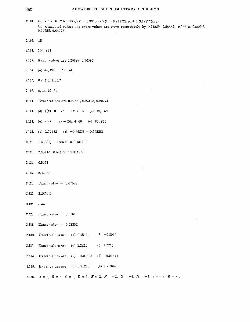
242 ANSWERS TO SUPPLEMENTARY PROBLEMS
2.101. (a) sin x = 2 . 8 0 6 5 6 ( x / ~ ) ~ - 6.33780(~/~)3 + 0 . 2 1 1 7 2 ( x / ~ ) ~ + 3.12777(x/~) ( b ) Computed values and exact values are given respectively by 0.25859, 0.25882; 0.96612, 0.96593; 0.64725, 0.64723
2.103. 15
2.104. 106, 244
2.105.
2.106. (a) 44, 202 ( b ) 874
Exact values are 0.25882, 0.96593
2.107. 6.2, 7.6, 11, 17
2.108. 8, 14, 22, 32
2.111. Exact values are 0.97531, 0.95123, 0.92774
2.113. ( b ) f(x) = 3x2 - 11% + 15 (c) 19, 159
2.114. (a) f ( x ) = x3 - 20% + 40 (b) 65, 840
2.121. (b) 1.32472 (c) -0.66236 2 0.56228i
2.122. 1.36881, -1.68440 k 3.43133i
2.123. 2.90416, 0.04792 * 1.311252'
2.124.
2.125.
2.126.
2.127.
2.128.
2.129.
2.131.
2.132.
2.133.
2.134.
2.135.
2.138.
0.5671
0, 4.9651
Exact value = 3.67589
2.2854%
3.45
Exact value = 0.2181
Exact value = 0.08352
Exact values are (a ) 0.4540 ( b ) -0.8910
Exact values are (a) 1.2214 (b) 1.2214
Exact values are (a) -0.31683 ( b ) -0.29821
Exact values are (a) 0.91230 ( b ) 0.72984
A = 6 , B = 8 , C = 6 , D = 3 , E = 2 , F = - 2 , G = - 4 , H z - 4 , J z - 2 , K = - 3

2.140.
2.141.
2.142.
2.143.
2.144.
2.145.
2.146.
2.148.
2.150.
2.151.
2.157.
2.158.
2.159.
2.160.
2.165.
2.166.
ANSWERS TO SUPPLEMENTARY PROBLEMS
Exact value = 3.80295
Exact values a re (a) 1.7024 (b) 2.5751
11.72 years
(a ) 0.9385 ( b ) 0.6796
Exact value = 22.5630
2.285%
(a) 38.8 (b) 29.4
Exact values are 0.74556, 0.32788, 0.18432, 0.13165, 0.08828, 0.05261
0.97834, 0.66190, 0.47590, 0.34600, 0.24857, 0.17295, 0.11329, 0.OG604, 0.02883
f ( % ) = p * + r + 1
Qk(k + 1)(2k + 1)
( a ) &k(k+ 1) ( b ) &V(k+ 1)2
ik(6k2 + 3k - 1)
( a ) 2k2 - 6k + 3 -+ 2h- ( b ) 1177
k = 10
All values of k
2.168. At
CHAPTER
3.55. (a)
( b )
(4
3.57. (a)
( b )
x = 6, f (x) = 0.68748 should be 0.68784
3
3x5 ; + d - x + c (d ) 2eZS - $3-42 + c 5 2
4 ~ 3 1 2 - 2 $ X 4 '3 + c 8 (e) 4 In (x - 2) + c
2" ( f ) f 0 $(Z sin 3% + cos 3%) + c
-4e-3r(x + 9) + c
2 sin x - x cos x + c
(c)
(d) +91nsz - Q x 3 l n x + & x 3 + ~
ixZ(1nx - 4) + c
243

244 ANSWERS TO SUPPLEMENTARY PROBLEMS
3.58. (a) 4% sin 2x - 3x2 cos 2% + & cos 2% + c
( b ) &ezz(4x3 - 6x2 + 6% - 3) + c
3.59. (a) In (e" + s inx) + c
+ C -1
( e ) zqG-=3j ( b ) 2 e f i ( f i - l ) + c
( c ) 6 cos $ + 6% sin - 3@ cos + c
x sin r(x - +h) 3-65. (a) 2 sin i r h 4 sin2 i r h
-x cos r(x - &h) h sin rx
h cos rx
( b ) 2 sin +rh + 4 sin2 ?ph
1 1 12 3.67. - - 2(n + 2)(n + 3)
x sin r(x - i h ) 3.72. (4 sin $rh + 4 sin2 +rh
-x cos r(x - $h) h sin rx
h cos rx
('1 2 sin &rh + 4 sin2 &rh
3.74.
3.75.
3.76.
3.78.
3.81.
3.82.
3.83.
3.84.
3.85.
B (a) @(n+ 1) (b) in (3n- 1)
(a) gn(n + l)(n + 2) (c) hn(4nz + 6% - 1)
( b ) *n(n + l)(n + 2)(n + 3) ( d ) n(3n2 + 6% + 1)
4n(2n - 1)(272 + 1)

ANSWERS TO SUPPLEMENTARY PROBLEMS 245
5 2n t 5 5 23 2n2 + 14% + 23 23 12 - 2(n + 2)(n + 3) ’ 12 ( b ) 480 - 4(n + 2)(n + 3)(n + 4)(n + 5 ) ’ A80 3’86’
3.89. &n(n -t. l ) (n + 2)(3n + 1)
21 1 1 1 ( b ) 90 - 6(2n + 1)(2n + 3)(2n + 5)
3.91. (a) y + lo (2n + 7)(2n + 6)(2n + 3)(2n + 1)(2n - 1)
11x2 + 19n 11 3’93’ (a) 6(2n+ 1)(2n+ 3) ( b ) 5
n + 2 3.94“ 2 - - 2 n
3.95. 3n(n + 1)(2n + 1)
3.104. &r(Q)
3.105. 8
r’(x+n+ 1) - = ~ - r (x + n + 1) ’ + r(x + 1) In general,
* 253 xz 1 = 8 5 - x4 + -- $8 - x ( b ) -1/30, 0 3.110. ( a ) &(x) = x - - + - - - 120 48 72 720 24 12 24 720’
3.111. -1130, 1/42, -lit30
1 1 3.114. (a ) ;i n2(n + 1 ) 2 ( b ) 30 n(n + 1)(2n + 1)(3n2 + 3n - 1)
3.115. 3Bo(2) - 4B,(z) + B2(x) + 2B3(x) + 5B4(x)
3.119. (a ) e4 = 0, e5 = -1/240 1 1 1 1 1
120 48 x + -xz - - 48 240 ( b ) E4(x) = $ 2 4 - 1 2 x 3 + 24 x, E5(x) = 1 x 5 - - 4
(c) E , = 5, E, = 0
3.125. P ( x 3 - Gx2 + 18x - 26)

246 ANSWERS TO SUPPLEMENTARY PROBLEMS
3.126. (n + 1)s cos 2(n + 1) - (3n2 + 9% + 7) cos 2(n + 2)
+ 6 ( n + 2 ) C O S ~ ( ~ + 3) - 6 C O S ~ ( ~ + 4) - cos2
+ 7 cos 4 - 12 cos 6 + 6 cos 8
3.132. &n2(2n4 + 6n3 + 5x2 - 1)
3.146. (a) r / 4 ( b ) r / 3 2 (c) r/fi
CHAPTER 4
4.40. (a) n2 (d ) Qn(n + l ) (n + 2) (9) &n(n + l ) (n + 2)(3n + 17)
(b) Qn(2n - 1)(2n + 1) (e) )+(n + 1)2 (h) Qn(3n3 + 46n2 + 255% + 596)
(c) an(6n2 + 3n - 1) (f) &(2n - l ) (2n + 1)(2n + 3)(2n + 5) + 9
x + l (1 - x)3 4.41. __-
4.43. 9/32
X x(x + 1) 3 4 6% - x2 4.44. (a) ___ (1 -x)2 p T p (1 - 4 3
4.45. 3591500
4.46. 5e - 1
4.48. (x4 - 7x2) sin x + (x - 6x3) cos x
4.49. $x cosh v% + f e ( 1 - k x ) sinh fi
4.59. Exact value = 1.09861
4.61. Exact value = 1
4.62. 0.63212

ANSWERS TO SUPPLEMENTARY PROBLEMS 247
4.64. ( a ) Qn(n + 1)(2n -f- 1) ( c ) +n(n + l ) (n + 2)
(a) &22(n + 1 ) 2 (d ) & R ( R + 1)(2n + 1)(3n2 + 3n - 1)
4.67. y = 0.577215
4.70. 1.20206
4.78. Exact value = 3,628,800
4.79. 2100/5fi - 4.036 X 1028
4.83. xe-s(2 - x)
11 6n + 11 11 (a) 180 - 12(2n+ 1) (2n+3)(2n+5) 180 4.84.
4.86. 1.092
4.88. (a) 1.0888
4.94. +(-l)n-ln(n + 1)
4.95. 29n2 - 2n + 3 ) - 3
4.99. ( a ) 1.09861 ( b ) 0.785398 (c) 0.63212
CHAPTER 5
5.60. (b) y = 5e5 - x2 - 2% - 2
5.61. Y(X) = 5(1 + h ) z / h - $2 + (h- 2 ) s - 2
5.63. y = 2 cos x + 5 sin x + 3x2 - 5x - 2
5.68. (a) 2f(x+2h) - 3 f ( x + h) + f(x) = 0 x2 x ( b ) f ( x + 3h) + 4f(x + 2h) - 5 f ( x + h) + 2j(x) = j-p - 4 ~ + 1
5.69. (a ) , (c), ( d ) , ( e ) , (f), (9) linearly independent; ( b ) , ( h ) linearly dependent
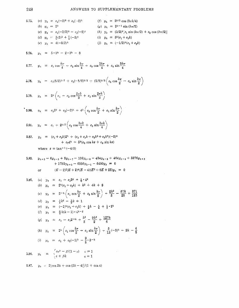
248 ANSWERS TO SUPPLEMENTARY PROBLEMS
ka kn 3kn 3kn 5.77. 2/lc = c1 cos- + c2 sin- + c3 cos- + c4 sin- 4 4 4 4
3 2 r k
3 5.79. Y k = 2k c1 + c2 cos- + c3 sin-
5.81. yk = c1 + Z k l 2
5.82. Z/k = (cl + c,k)2k -I- (c, + c,k + ~ 5 k 2 4- Cgk3)(-2)k + c,4k + 5 k ( c , cos ke + cg sin ke)
where e = tan-l(-4/3)
kn
5.87. y k = ~ [ C O S 2k + cos (2k - 4)]/(1 4- cos 4)

ANSWERS TO SUPPLEMENTARY PROBLEMS 249
k2 6 7 k 422 4 * 3 k - - + - - - - - 5.89. y k = c12k + ~ 2 ( - 2 ) ~ + 2k + c4 sin- 2 15 225 3375 65
5.90. y k = c l ( - l ) k + c2 c o s i kr + c3 sin- kir + 2k [8 cos (3k - 9) + cos 3k] 3 3 65 + 16 cos9
irk 5.94. yk = ~ 1 ( - 6 ) k + c22k + 2 5 f i s i n 3 - 105 cos- 258
k2 8k 38 3 9 27 5.95. ( c ) ylc = C12k + C,4k - 3k + - + - + -
( b ) yk = C, + c,k + k2 + $k3 + 1 * 4 k 9 kn k7i (f) uk = c1 COS- + cp sin- ( c ) yk = (el +'c&+ 3 k 2 ) z p k 3 3
k7i k7i (-1)" ( d ) yk = c1 cos- + c2 sin- + 3 - 2 2 ,.=O k + 2~
-(r + 1) sin 3 1
1
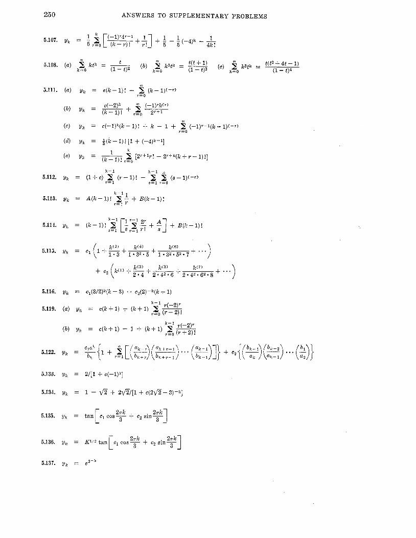
250 ANSWERS TO SUPPLEMENTARY PROBLEMS
2 4 1 + c(-l)k]
1 - fi + 2 f i / [ l + ~ ( 2 f S - 3) -k ]
2-k 2tik tan c1 cos- + c2 sin- L - 3 3
1

ANSWERS TO SUPPLEMENTARY PROBLEMS 251
5.150. (a) et
5.153. Z C ( X , y) = ( - 2 ) x F ( ~ + 21)
5.158. uk,,, = F ( 2 k - m ) - 2 k - m t 1
5.160. u k , m = 2 k F ( k - m ) + G ( k - m ) + 2, ,H(k-m)
5.161. uk,nz = F ( k - m )
7k rrk nm rrm F ( k - m) cos 2 + G(k - m) sin - + H ( k - m) cos - + J ( k - m) sin - 3 3 3 3 5.162. uk,m =

252 ANSWERS TO SUPPLEMENTARY PROBLEMS
5.167. (c) y = CO x4 x7
1 .3 5.**(k- 1) 2 4 6.m.k~ k even Y k
5.183. U k , m = F ( k + m ) + kG(k+m) + k2H(k+m)
5.184. uk,m = 8: = Stirling numbers of the first kind
5.185. U k , m = sk = Stirling numbers of the second kind
5.188. Y(x) = (x - l ) /e
x2 - 4% + 1 -t- 2x tan 1 cos 1 5.189. Y ( x ) =
( - l ) k - 1 +- 1 5.190. u k - - - + - - . . . l! 2 ! 3 ! k!
5.191. (a) u(x, y) = A(3x + 2y)2 + e - ( 3 2 * 2 ~ ) / 2
5.192. (a) U ( X , Y ) = x2 + y + Q X Y
CHAPTER 6
f l - 1 1 - a k 1 - f i
l + f i 6.62. (a ) 7 ( - a k + l ) where a = -

A N S W E R S TO SUPPLEMENTARY PROBLEMS 253
6.68. 2
6.71. (a ) Tg(5) = 2x2-11, T~(x) = 6 ~ 3 - 3 3 ~ , T~(x) = 8 x 4 - 8 x 2 + 1
6.75. (a) A k + l = Ak f iAk ( b ) A , = P(1+ i ) k
6.76. A , + l - (1 + i )A, = S
an [(1+ i)" - 11 - T a + si 6.77. A,+1 - (1 + i )A , = S + nu, A , = - i 2
1 1 6.89. - - - 2 ! 3 !
2 6.91. (a) +
6.92. - b + b + r
b b S r 6.93. -
6.102. (a) Exact value = 1.7974
441 256 6.104. (a) Exact value = - = 1.72265625
6.109. ( b ) Exact value = 1.1487
6.112. Exact values: x(0.5) = 0.645845 ~ ( 0 . 5 ) = 0.023425
6.113. u=o
u = o u = o
U1 = 0.071428571,
Us = U1, U4 10.1875, Us = 0.2500,
UB = Uq, U8 = 0.526785714,
Uz = 0.098214285,
U , = 0.428571428,
Ug = U7
U = l

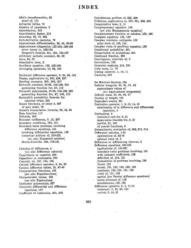
I N D E X
Abel’s transformation, 85
Actuarial tables, 75 Algebra of operators, 2 Amortization, 215 Amortization factor, 215 Annuities, 55, 75, 228 Anti-derivative operator, 79 Approximate differentiation, 39, 40, 60-62 Approximate integration, 122-124, 129-136
error terms in, 132-134 Gregory’s formula for, 124, 134-137
proof of, 101
Arbi t rary periodic constant, 82, 93 Area, 80, 92 Associative laws, 2 Auxiliary equation, 153, 165-168 Averaging operators, 10, 88, 108
Backward difference operator, 9, 24, 25, 124 Beams, applications to, 200, 206, 207 Bending moments, 200, 206, 207 Bernoulli numbers, 86-88, 105-108, 234
generating function for, 87, 110 Bernoulli polynomials, 86-88, 105-108, 235
generating function for, 87, 109, 110 Bernoulli’s probability formula f o r
Bessel functions, of order k, 227 of zero order, 75
Bessel’s interpolation formula, 36, 48, 50 Beta function, 117 Billiards, 208 Binomial coefficients, 9, 13, 227 Boundary conditions, 150, 151 Boundary-value problems, involving
repeated trials, 225
difference equations, 151 involving differential equations, 150 numerical solution of, 219-221
Sturm-Liouville, 158, 178-181 [see also Numerical solution]
Calculus of differences, 4
Capacitance or capacity, 200 Capacitors o r condensers, 200 Casorati, 54, 157, 164, 165 Central difference operator, 9, 24, 25 Central difference tables, 35, 47-49 Characteristic functions, 158
[see also Eigenfunctions] Characteristic values, 158
[see also Eigenvalues] Chebyshev polynomials, 227 Clairaut’s differential and difference
Coefficient of restitution, 201, 208
[see also Difference calculus]
equations, 197
Coincidences, problem of, 228, 229 Collisions, applications to, 200, 201, 208, 209 Commutative laws, 2, 13 Complementary equation, 168
Complementary function or solution, 155, 160 Complete equation, 153, 155 Complex numbers, conjugate, 153
polar form of, 153, 154 Complex roots of auxiliary equation, 153 Conditional probability, 201 Conservation of momentum, 201 Continued fraction, 226 Convergence, intervals of, 8 Convolution, 193 Corrector methods, 218, 230 Cube roots, 11, 75 Cubing operator, 1, 10, 11 Currents, 200
[see also Homogeneous equation]
De Moivre’s theorem, 154 Definite integrals, 80, 81, 91, 92
approximate values of [see Approximate integration]
Definite sums, 83, 84, 96, 97 Density o r weight, 159 Dependent events, 201 Derivative operator, 1, 3, 10, 14, 15
relationship of to difference and differential operators, 4
Derivatives, 3 Leibnitz’s rule for, 9, 24 mean-value theorem for, 8, 27 partial, 81, 160 of special functions, 5
Determinants, evaluation of, 202, 213, 214 Difference calculus, 1-31
applications of, 32-78 general rules of, 5
Difference or differencing interval, 2 Difference equations, 150-198
applications of, 199-231 boundary-value problems involving, 151 with constant coefficients, 152 definition of, 150, 151 formulation of problems involving, 199 linear, 152 mixed, 159, 182, 183, 188, 189 nonlinear, 152, 159, 181, 182 order of, 151, 152 partial [see Partial difference equations] series solutions of, 158 simultaneous, 159, 182
backward, 9, 24, 25, 124 central, 9, 24, 25
Difference operator, 2, 3, 11-14

INDEX
Difference operator (cont.) forward, 9 relationship of to differential and derivative
second and nth order, 3 operators, 4
Difference and sum of operators, 2 Difference tables, 23, 32, 33, 40-42
Differences, calculus of, 4 central, 35, 47-49
central, 9, 24, 25, 35, 47-49 leading, 33 Leibnitz’s rule for, 9, 24 of polynomials, 33 of special functions, 7 of zero, 26
Differentiable functions, 1, 10 Differential, 3, 4 Differential calculus, 4 Differential-difference equations, 159, 182 Differential equations, 150, 161
boundary-value problems involving, 150 as limits of difference equations, 151, 152,
162, 163 numerical solution of, 202, 215-221 order of, 150 partial [serz Part ia l differential equations]
relationship of to difference and derivative Differential operator, 3, 4, 14, 1 5
operators, 4
general rules of, 4, 5 of a n integral, 81, 84, I l l of sums, 84, 97
Diagamma function, 86, 104, 105 Distributive law, 2 Divided differences, 38, 39, 66-69 Doubling operator, 1
Differentiation, approximate, 39, 40, 60-62
e, 5 Eigenfunctions, 158, 178, 179
expansions in series of, 169, 179, 180 mutually orthogonal, 169, 178
Eigenvalues, 158, 178, 179 reality of, 158, 179
Elastic collisions, 201 Electrical networks, applications to, 200,
205, 206 Equality of operators, 1 Error function, 70 Error term, in approximate integration
formulas, 123, 132-134 in Euler-Maclaurin formula, 125, 137-140
error term in, 125, 137-140 evaluation of integrals using, 124
Euler method, 216 modificd, 217
Euler numbers, 88, 89, 108, 109, 236 Euler polynomials, 88, 89, 108, 109, 237
Euler transformations, 148 Euler’s constant, 85, 117
Euler-Maclaurin formula, 124, 136, 137
generating function for, 89
Events, dependent and independent, 201
Everett’s formula, 77 Expected duration of a game, 226 Exponents, laws of, 2
mutually exclusive, 201
Factorial functions, 5 , 6, 16-20
Factorial polynomials, 6 Factorization of operators, 158, 176 Fa i r game, 211 Families of curves, one- and
two-parameter, 197 Fibonacci numbers, 202, 211, 212, 238
Finite differences, 4 Flrxural rigidity, 206 Fluid flow, 221 Forecasting, 34 Forward difference operator, 9 Fourier series, 118 Frequency, 199, 202-205
Gamma function, 6, 70, 76, 85, 86, 102-105 Gauss’ interpolation formulas, 36, 50
General solution, of a difference equation, 151, 161, 162
generalized, 7
table of, 238
derivation of, 49
of a differential equation, 150, 161 of a partial difference equation, 160
Generalized hterpolation formulas, 36 Generating function, for Bernoulli
numbers, 87, 110 for Bernoulli polynomials, 87, 109, 110 for Euler polynomials, 89 method for solving difference equations,
167, 158, 174, 175, 183, 184, 186, 187 Gravity, vibrating string under, 221 Gregory-Newton backward difference
formula, 36, 48, 49 derivation of, 48
Gregory-Newton formula, 9, 21-24, 36, 42-47 inverse interpolation by means of, 59, 60 with a remainder, 9, 22, 23 in subscript notation, 34 used in approximate integration,
122, 129, 130 Gregory-Ncwton forward difference formula
Gregory’s formula for approximate
Grid. 219
[sce Gregory-Newton formula]
integration, 124, 134-137
Heat flow, 221 [see also Steady-state temperature]
Homogeneous linear difference equations, 153 with constant coeficients, 153, 165-168 in factored form, 153
Identity or unit operator, 1 Indefinite integrals, 79 lndependent events, 201 Index law, 2
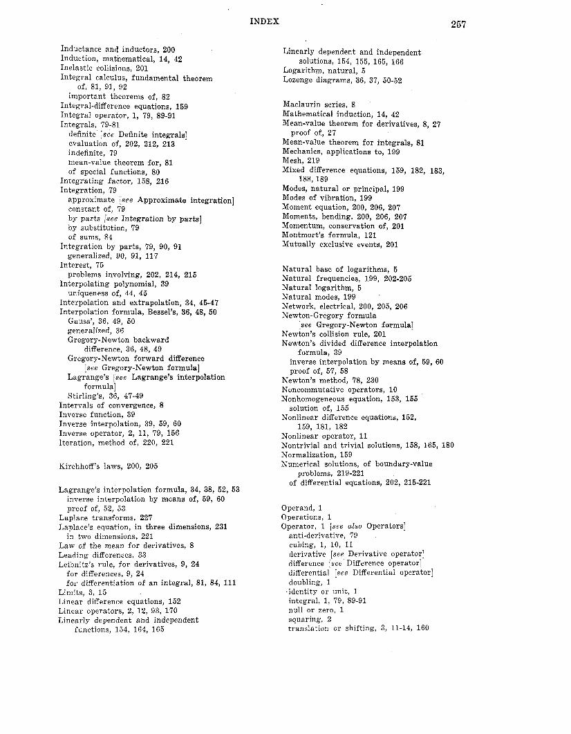
INDEX 257
Inductance and inductors, 200 Induction, mathematical, 14, 42 Inelastic collisions, 201 Integral calculus, fundamental theorem
of, 81, 91, 92 important theorems of, 82
Integral-difference equations, 159 Integral operator, 1, 79, 89-91 Integrals, 79-81
definite [ see Definite integrals] evaluation of, 202, 212, 213 indefinite, 79 mean-value theorem for, 81 of special functions, 80
Integrating factor, 158, 216 Integration, 79
approximate [see Approximate integration] constant of, 79 by par ts [see Integration by parts] by substitution, 79 of sums, 84
generalized, 90, 91, 117
problems involving, 202, 214, 215
uniqueness of, 44, 45
Integration by parts, 79, 90, 91
Interest, 75
Interpolating polynomial, 39
Interpolation and extrapolation, 34, 45-47 Interpolation formula, Bessel’s, 36, 48, 50
Gauss’, 36, 49, 50 generalized, 36 Gregory-Newton backward
Gregory-Newton forward difference
Lagrange’s [see Lagrange’s interpolation
Stirling’s, 36, 47-49
difference, 36, 48, 49
[see Gregory-Newton formula]
formula]
Intervals of convergence, 8 Inverse function, 39 Inverse interpolation, 39, 59, 60 Inverse operator, 2, 11, 79, 156 Iteration, method of, 220, 221
Kirchhoff’s laws, 200, 205
Lagrange’s interpolation formula, 34, 38, 52, 53 inverse interpolation by means of, 59, 60 proof of, 52, 53
Laplace transforms, 227 Laplace’s equation, in three dimensions, 231
in two dimensions, 221 Law of the mean f o r derivatives, 8 Leading differences, 33 Leibnitz’s rule, for derivatives, 9, 24
for differences, 9, 24 f o r differentiation of a n integral, 81, 84, 111
Limits, 3, 15 Linear difference equations, 152 Linear operators, 2, 12, 93, 170 Linearly dependent and independent
functions, 154, 164, 165
Linearly dependent and independent solutions, 154, 155, 165, 166
Logarithm, natural, 5 Lozenge diagrams, 36, 37, 50-52
Maclaurin series, 8 Mathematical induction, 14, 42 Mean-value theorem for derivatives, 8, 27
Mean-value theorem for integrals, 81 Mechanics, applications to, 199 Mesh, 219
proof of, 27
Mixed difference equations, 159, 182, 183, 188,189
Modes, natural o r principal, 199 Modes of vibration, 199 Moment equation, 200, 206, 207 Moments, bending, 200, 206, 207 Momentum, conservation of, 201 Montmort’s formula, 121 Mutually exclusive events, 201
Natural base of logarithms, 5 Natural frequencies, 199, 202-205 Natural logarithm, 5 Natural modes, 199 Network, electrical, 200, 205, 206 Newton-Gregory formula
Newton’s collision rule, 201 Newton’s divided difference interpolation
[see Gregory-Newton formula]
formula, 39 inverse interpolation by means of, 59, 60 proof of, 57, 58
Newton’s method, 78, 230 Noncommutative operators, 10 Nonhomogeneous equation, 153, 155
solution of, 155 Nonlinear difference equations, 152,
159, 181, 182 Nonlinear operator, 11 Nontrivial and trivial solutions, 158, 165, 180 Normalization, 159 Numerical solutions, of boundary-value
of differential equations, 202, 215-221 problems, 219-221
Operand, 1 Operations, 1 Operator, 1 [see also Operators]
anti-derivative, 79 cubing, 1, 10, 11 derivative [see Derivative operator] difference [ see Difference operator] differential [see Differential operator] doubling, 1
.identity o r unit, 1 integral, 1, 79, 89-91 null o r zero, 1 squaring, 2 translation o r shifting, 3, 11-14, 160

INDEX
Operator methods, for solving difference equations, 156, 169-172, 187
for summation, 85, 101, 102 symbolic / see Symbolic operator methods]
algebra of, 2 associative laws for , 2 averaging, 10, 88, 108 definitions involving, 1, 2 distributive law for , 2 equality of, 1 factorization of, 158, 176 inverse, 2, 11, 79, 156 linear, 2, 12, 93, 170 noncommutative, 10 nonlinear, 2 partial difference, 160 product of, 2 sum and difference of, 2
of a differential equation, 150 reduction of, 157, 173, 174
Orthogonal functions, 159, 178 Orthonormal set, 159
Operators, 1, 10, 11 [see also Operator]
Order, of a difference equation, 151, 152
Part ia l derivative, 81, 160 Part ia l difference equations, 160, 184-187
Part ia l difference operators, 160 Part ia l differential equations, 160, 188
numerical solutions of, 218-221 Partial fractions, 192 Part ia l translation operators, 160 Particular solutions, of a difference
of a differential equation, 150, 161 methods of finding, 155
solutions of, 160
equation, 151, 166, 167
Pascal’s triangle, 227 Payment period, 214 Periodic constant, 82, 93 Points, problem of, 211 Poisson’s equation, 231 Polar coordinates, 102, 117 Potential theory, 221 Power series, 121, 122, 127-129 Prediction o r forecasting, 34 Predictor-corrector methods, 218, 230 Principal, 75, 214 Principal modes, 199 Probability, applications to, 201, 202, 209-211
conditional, 201 Product of operators, 2
Real roots of auxiliary equation, 153 Rectangular coordinates, 103 Reduced equation, 153, 168
Reduction of order, 157, 173, 174 Repeated trials, probability formula for, 225 Resistance and resistor, 200 Restitution, coefficient of, 201, 208 Rolle’s theorem, 26
[see also Homogeneous equation]
Roots, of auxiliary equation, 153, 154 of equations, 58, 59 Newton’s method for finding, 78
Sequences and series, general terms of, 34, 43, 44 [see also Series]
uniqueness of, 43, 44
of constants, 121, 126 of eigenfunctions, 159, 179, 180 intervals of convergence for, 8 Maclaurin, 8 power, 121, 122, 127-129 summation of, 97-100, 121, 142, 143
[see also Summation] Taylor [see Taylor series]
Series, 8
Series solutions of difference equations, 158 Shifting or translation operator, 3, 11-14, 160 Simply supported beams, 200, 206, 207 Simpson’s one-third rule, 122
error term in, 123, 133, 134 proof of, 131
error term in, 123 proof of, 132
Simpson’s three-eighths rule, 123, 132
Simultaneous difference equations, 159, 182 Solution, of a difference equation, 150
of a differential equation, 150 nontrivial and trivial, 158, 165, 180
Springs, vibrations of, 223 Squaring operator, 28 Steady-state temperature in a plate, 221, 231 Step by step method, 216 Stirling numbers, 6, 7, 20, 21
of the first kind, 7, 20, 232 recursion formulas for, 7, 20, 21 of the second kind, 7, 20, 21,86, 106,230,233
proof of, 141
derivation of, 49
rotating, 223 tension in, 202 vibrations of, 199, 202-205
Stirling’s formula for n ! , 125, 140-142
Stirling’s interpolation formula, 36, 47, 48
String, under gravity, 221
Sturm-Liouville boundary-value problem, 158 Sturm-Liouville difference equations, 158,
Subscript notation, 32, 40, 84
Sum calculus, 79-120
178-181
use of in difference equations, 152, 163, 164
applications of, 121-149 fundamental theorem of, 83, 84, 96-98, 100
Sum and difference of operators, 2 Sum operator, 82, 92-95 Summation, 82
general rules of, 82, 92-95 operator methods for, 85, 101, 102 by parts [see Summation by parts] of series, 97-100, 121, 142, 143 of special functions, 83 theorems using subscript notation, 84 using subscript notation, 100

INDEX
Summation factor, 158, 174, 176 Summation by parts, 82, 149
generalized, 116 proof of, 94
indefinite, 82 Sums, definite, 83, 84, 96, 97
Superposition principle, 154, 166, 168 Symbolic operator methods, 8
differentiation formulas obtained by, 60, 61 Gregory-Newton backward difference
Gregory-Newton formula obtained by, 24 formula obtained by, 48
Synthetic division, 6, 18
Tables, central difference, 35, 47-49 divided difference, 38 location of errors in, 64, 65 with missing entries, 38, 53-56
Tangent numbers, 89, 120 Taylor series, 8
in operator form, 8 solution of differential equations by, 231
Taylor’s theorem or formula, 8 Temperature, steady-state, 221, 231 Tension, in a string, 202 Three-moment equation, 200 Torsion constant, 223 Torsional vibrations, 223
Trial solution, 155, 156 Trivial and nontrivial solutions, 158, 165, 180
Undetermined coefficients, method of, 155, 156, 168, 169, 187
Variable coefficients, linear difference equations with, 157, 158, 175-178
Variation of parameters, 156-158, 172, 173, 175 solution of first-order linear difference
equations by, 175 Vectors, 159, 180 Vibrating systems, applications to, 199,202-205 Vibration, 199
frequencies of, 199, 202-205 modes of, 199 of springs, 223 of a string [see String] torsional, 223
Wallis’ product formula, 141, 149 Wave equation, 222 Weddle’s rule, 123, 143, 144
error term in, 123 proof of, 143
Weight or density, 159 Wronskian, 154
Translation o r shifting operator, 3, 11-14, 160 Trapezoidal rule, 122, 123, 130
error term in, 123, 132, 133 proof of, 130
Yoling’s modulus of elasticity, 206
Zig-zag paths, 36, 37, 50-52


Catalog
If you are interested in a list of SCHAUM’S OUTLINE SERIES send your name and address, requesting your free catalog, to:
SCHAUM’S OUTLINE SERIES, Dept. C
1221 Avenue of Americas New York, N.Y. 10020
McGRAW-HILL BOOK COMPANY


