
1
Financial Conflicts of Interest in Medicine*
Joseph Engelberg
Christopher A. Parsons
Nathan Tefft
January 2014
Abstract: We use the geographic distance between a doctor’s office and drug company headquarters to instrument for the likelihood of pecuniary transfers, such as meals or speaking fees. Doctors tilt prescriptions in favor of the paying firm’s drugs, shifting away from both branded and generic substitutes. Larger transfers cause larger shifts in prescriptions. We explore two potential explanations: 1) information flow (or its perception), and 2) rent seeking. Payments increase prescriptions of branded drugs over generic equivalents, situations where information cannot play a large role. However, doctors residing in states known to be corrupt in other ways (e.g., electoral fraud) are much more sensitive to payments from the drug industry, as are male doctors.
* We have benefited from discussions with Anirban Basu, Daniel Carlat, Doug Conrad, Raymond Fisman, Dan Hamermesh, Ryan Hansen, Sheridan Titman and seminar participants at Harvard University, the University of Southern California, and the University of Washington. ‡ Contact: Joseph Engelberg, Rady School of Management, University of California at San Diego, (Email) [email protected] (Tel) (1) 858-822-7912; Christopher A. Parsons, Rady School of Management, University of California at San Diego, (Email) [email protected] (Tel) (1) 858-534-8782; Nathan Tefft, School of Public Health, University of Washington, (Email) [email protected] (Tel) (1) 206-221-5897.
2
I. Introduction
When an informed buyer enlists the help of an expert, conflicts of interest often
arise. Take for example a wine sommelier working at a fine restaurant. Is the
recommended Pinot Noir the optimal pairing, or has the restaurant encouraged the
sommelier to push a particular brand, perhaps trying to rid itself of a few extra bottles?
While rent-seeking behavior may not be surprising generally, that financial
conflicts of interest could influence physicians’ advice might be less expected. For one,
doctors are highly paid, with most falling in the top 5% of the income distribution within
the US (U.S. Bureau of Labor Statistics, 2010; U.S. Census Bureau, 2010). Moreover,
intrinsic motivation is thought to be important in medicine, with the goal of maximizing
patient health a paramount objective (Heyes, 2005; Rebitzer and Taylor, 2011).
On the other hand, this need not coincide with the objectives of pharmaceutical
firms, who have strong incentives to maximize prescriptions. Consequently, when drug
companies have financial relationships with physicians, medical decisions may be
influenced by pecuniary motives not directly related to patient health.
This possibility has not gone unnoticed by legislators. Beginning in 2014, the
Physician Payments Sunshine Act took effect, when drug and medical device
manufacturers will be required to publicly report payments to physicians and teaching
hospitals (Centers for Medicare & Medicaid Services, 2013). A presumption underlying
this legislation is that transfers from the medical industry create conflicts of interest for
providers that, in turn, influence their behavior. This paper evaluates that presumption.
We have three goals. First, using micro-level data on payments to individual
physicians and their prescriptions, we explore whether a positive association exists at all.
Second, we seek to understand whether payments exert a causal influence on physician
behavior, or whether omitted doctor, firm, or even doctor-firm match attributes create

3
spurious correlation. Finally, provided that a causal relation does appear to exist, we dig
deeper into the mechanism. For example, do drug companies use marketing dollars to
educate physicians, thereby allowing them to make more informed decisions? Or, is
simple rent-seeking a better explanation?
To address these questions, we collect data on payments to physicians provided
on the Dollars for Docs website, hosted by independent journalist consortium
ProPublica (ProPublica, 2013a). Dollars for Docs is a searchable web interface allowing
a user to observe transfers from pharmaceutical firms to specific physicians. In 2011,
twelve companies reported payments, including most of the major firms including Pfizer,
Merck, GlaxoSmithKline, AstraZeneca, and Johnson & Johnson. Although reporting is
not standardized (yet, see above), most firms break down payments by dollar amount
and type, such as gifts, meals, speaking, travel, consulting, and on occasion, proprietary
research.
With this dataset we merge prescription information for each doctor as reported
from Medicare (Part D) reimbursements, also provided by ProPublica on its Prescriber
Checkup website (ProPublica, 2013b). This combination allows us to conduct cross-
sectional regressions comparing prescribing patterns of doctors who differ in whether, or
how much, they are paid by a given drug company.
Our sample is comprised of some 334,000 doctors, over half of all physicians
licensed in the U.S. Pairing each doctor i in our sample to each of the twelve
pharmaceutical firms j, we ask whether j to i transfers are associated with more
prescriptions for company j’s drugs written by doctor i. We find a positive association
that scales with transfer size. Small payments (e.g., under $1000 for the year) are
associated with about twenty additional prescriptions. This increases to almost sixty
when the transfer exceeds $1000.

4
This payment-prescription pattern survives both doctor and company fixed
effects, meaning that neither unobserved attributes of doctors nor drug companies can
drive the relation. It remains possible, however, for omitted heterogeneity in doctor-
firm matches to generate spurious correlations between payments and prescriptions.
For example, consider a physician who specializes in a condition for which
relatively few treatments are available, such as Alzheimer’s disease. When a new drug is
brought to market (take Novartis’s introduction of Exelon for dementia in 2007 as an
example), such specialist physicians are likely valuable sources of information about side
effects, patient compliance, and so on. In these cases, payments from drug companies,
say, in the form of meals or consulting, are not causally related to prescribing behavior.
Ruling out such unobserved doctor-firm heterogeneity requires exogenous
payments to physicians, which are uncorrelated with their counterfactual prescription
patterns absent transfers from drug companies. We approximate this ideal scenario
using the geographical distance between each doctor’s office and the headquarters of
each drug company. Intuitively, the idea is that doctors located closer to a firm’s
headquarters are more likely to be in contact with its sales force – doctors near
Indianapolis probably encounter more Eli Lilly drug representatives than their peers in
St. Louis – but due to proximity, rather than unobserved determinants of prescribing
behavior.
Indeed, in first stage regressions, we find that both the incidence and amount of
transfers declines monotonically with the distance between a doctor’s office and firm
headquarters (see Figure 2). When we instrument for payments using doctor-firm
distance in the second stage, we continue to find a strong, positive relation between
transfers and prescriptions. The IV models also survive doctor and firm fixed effects,

5
meaning that identification is achieved by comparing the relative distance between
multiple firms for the same doctor.
Our remaining analysis takes as given a causal relation between drug company
payments and physicians’ prescription choices, and attempts to better identify the
mechanism. There are three possibilities, which are not mutually exclusive. First,
doctors may become better informed via interactions with drug companies, which may
alter prescribing behavior. Second, doctors may simply think they have become better
informed, but in reality, have not. We refer to these possibilities, respectively, as
“informative persuasion” and “non-informative persuasion.” The final possibility is rent
seeking, whereby doctors tilt prescriptions toward firms from which they derive
pecuniary benefits, either present or expected.
To evaluate the persuasion hypotheses, we measure the payment-prescription
effect among subsamples where information flow should play a reduced role relative to
the entire sample. Our first such comparison is between Astrazeneca’s Crestor and
Pfizer’s Lipitor, twin cholesterol-reducing blockbusters in the “statin” class. Both drugs
are widely prescribed to large cross-sections of the American population, making it less
likely that unobserved differences in patient attributes generate meaningful differences
between doctors. Yet, in head-to-head comparisons, we find that payments from Pfizer
tilt the balance in favor of Lipitor (with larger payments having a bigger effect), with
transfers from AstraZeneca being associated with more prescriptions of Crestor.
The second subsample we analyze eliminates entirely the ability for persuasion
(informative or non-informative) to generate correlation between payments and
prescriptions. We compare a number of branded drugs to their generic equivalents, i.e.,
not simply drugs in the same drug class. That we find a positive payment-prescription
relation here is even more challenging to attribute to information flow from drug

6
companies, even for the most uninformed (hypothesis 1 above) or naïve (hypothesis 2)
doctors.
We conclude by considering in more detail the possibility that physicians are
susceptible to rent seeking. As for the other alternatives, we examine subsets of the data
where the effects of corruption, if true, should be strongest. Our first test uses data on
federal convictions of corruption-related crime (Glaeser and Saks, 2006) to proxy for the
corruption rate of each U.S. state. Comparing the least corrupt U.S. states (e.g.,
Minnesota, Oregon, Nebraska) to the most corrupt (e.g., Louisiana, Mississippi, Illinois),
we find that the prescription-payment magnitude is cut by nearly half. This is
particularly striking given that the most corrupt states are among the poorest (many in
the Southeast), and yet the ratio of branded-to-generic drugs is highest in precisely this
region (see Figure 4).
The second test is between male and female doctors. Using an algorithm to
classify doctor first names by gender, we find that men are over twice as sensitive to
payments as women. This confirms experimental and field evidence suggesting that
women are, on average, more honest and less corruptible than men (e.g. Dollar et al.,
2001).
Our findings provide an empirical benchmark for assessing the impact of the
upcoming Sunshine Act of 2014, given that our sample predates its implementation by
four years and even most discussion by two years. Although only a portion of our
analysis can distinguish between persuasion and rent-seeking behavior, these
mechanisms need not be separated in order for the Sunshine Act to be warranted.
Specifically, if either potentially welfare-reducing phenomenon exists, then its effects
may be ameliorated by the legislated transparency of pharmaceutical firm payments.

7
The idea that physicians face potential conflicts of interest is not new (American
College of Physicians, 1990; Medicare Payment Advisory Committee, 2009). For
example, well after ethical standards describing appropriate relationships between
pharmaceutical firms and physicians were developed, there was substantial concern that
payments affect or reward clinical behavior (Coyle, 2002). Controversy remains in part
because existing empirical evidence characterizing pharmaceutical industry and
physician relationships relies exclusively on opinion surveys (Madhavan et al., 1997;
Wazana, 2000; Katz et al., 2010), rather than on directly observed clinical behavior.
Notable exceptions include Larkin et al. (2012), which identifies a causal effect of
detailing on prescriptions using changes in hospital policies in six metropolitan areas,
and Pham-Kanter et al. (2012) which compares prescription behavior at the state level
between states which disclose pharmaceutical payments and those which do not. The
critical component of our study is the availability of both prescription and payment data
for over 330,000 individual physicians in every U.S. state, a breadth which not only
allows us to identify an effect of individual payments on individual prescriptions, but
also helps us specify the mechanism which generates the effect.
The remainder of the paper is organized as follows. In Section II, we describe
our payment and prescription data and provide summary statistics. Section III provides
evidence of a positive relationship between payments and prescriptions, while Section IV
explores potential mechanisms for the patterns we observe. We conclude in Section V.
II. Data
We draw on several data sources to study the relationship between industry
payments and physician prescribing behavior. First, we construct a listing of payments
from pharmaceutical firms to doctors using ProPublica’s Dollars for Docs

8
database(ProPublica, 2013a). ProPublica is an investigative journalism newsroom that
makes data available on industry payments and prescribing patterns. Dollars for Docs is
an online, searchable database of payments that were made publicly available by
pharmaceutical firms either voluntarily or due to legal settlements. The data begin in
2009, and we downloaded all data between 2009 and 2011 for our study. Data for twelve
pharmaceutical firms were available during this time period. Each observation in the
dataset is from a named pharmaceutical firm to a named provider and includes time
period (year), payment type, and specific or categorical dollar amount.
Table 1 lists several summary statistics of reported payments to providers
separated by pharmaceutical firm in Panel A and reported payment type in Panel B.
Reporting is voluntary or arising from legal settlements and is, therefore, somewhat
idiosyncratic. Inspection of Table 1 suggests these idiosyncrasies explain much of the
variation across pharmaceutical firms in the number of providers that receive payment.
For example, Merck only reported payments made for speaking over the 2009 - 2011
period. Because payments for speaking are less common, we identify approximately
2,000 providers to which Merck made payments annually.
On the other hand, AstraZeneca began reporting only speaking fees in 2010, but
increased its scope for reporting to include meals, gifts, consulting, research and travel in
2011. This expanded disclosure by AstraZeneca increased the number of providers
receiving payment from 2,381 in 2010 to 116,643 in 2011. Looking at the last row of
Panel A, it is clear that the total dollar amount of payments made by pharmaceutical
firms increased substantially, from $188.86 million in 2009 to $773.05 million in 2011,
but this increase was driven primarily by expanded disclosure (as in the AstraZeneca
example), rather than a dramatic increase in actual payments made.

9
The average dollar amount and prevalence of payments also varies considerably
by type of payment. For example, most reported research payments were greater than
$10,000, but they were relatively infrequent. Reported consulting, speaking, and travel
payments were also large, with many payments in those categories in the thousands. In
contrast, the median reported payments for gifts and meals were $72 and $37,
respectively, and reported meal payments were by far the most frequent, comprising
more than three-quarters of all reported payments.
ProPublica also provides a database of prescribing patterns called Prescriber
Checkup (ProPublica, 2013b). Prescriber Checkup is a searchable database of health care
providers and the number of Medicare Part D prescriptions (including refills) they wrote
for specific drugs in 2010 when that provider’s number of such prescriptions exceeded
50. This restriction was imposed to protect patient confidentiality. These data comprise
the universe of such provider-prescription information for the U.S. in 2010.
ProPublica aggregated these data from 2010 Medicare Part D insurance claims
that were obtained from the Centers for Medicare and Medicaid Services under a
Freedom of Information Act request. The unit of observation in the Prescriber Checkup
database is (Doctor, Drug), so for each doctor we know how many Medicare Part D
prescriptions she wrote for each drug (provided she wrote at least 50). We use drug
names to match drugs to their appropriate pharmaceutical firm (e.g., Lipitor matches
with Pfizer). Of the 1,685 drugs in the Prescriber Checkup database, 239 match to one of
our twelve pharmaceutical firms.
The Prescriber Checkup database also includes summary information by doctor
including the total number of Medicare Part D claims, the total number of patients
receiving at least one claim, and identifying information such as name, city, state and
medical specialty. We downloaded the Prescriber Checkup database and used the
10
identifying information to match providers from the Prescriber Checkup database to the
Dollars for Docs database. Table 2 provides some summary statistics from the matched
sample. Of the 334,086 doctors in the Prescriber Checkup database we identify 192,484
(58%) as having received at least one payment from our twelve pharmaceutical firms
between 2009 and 2011. Panel A of Table 2 also suggests that doctors who are paid by
pharmaceutical firms are more active than those who are not.
For example, the average doctor in our sample generated 2,980 Medicare Part D
claims in 2010 from 217 patients (13.7 claims per patient). However, doctors who
received payments from pharmaceutical firms generated 3,566 claims and saw 243
patients (14.7 claims per patient). Prescription rates are also higher for paid physicians
among branded claims, i.e. prescriptions for drugs made by our twelve pharmaceutical
firms. Panel A indicates that the average doctor generates 192 branded claims (0.88 per
patient) but a paid doctor generates 258 branded claims (1.06 per patient).
Panel B of Table 2 provides summary statistics for (Doctor, Firm) pairs, which is
the unit of observation in our main analysis. We choose (Doctor, Firm) rather than
(Doctor, Drug) as the appropriate unit because we are unable to observe whether a
payment was made to a doctor in connection with a specific drug; rather, we only
observe total payments by each drug company to each doctor. Panel B indicates that we
observe payments to doctors 11% of time among the over 4 million observations. When a
payment is observed, the average size is $1,766 with a standard deviation of $21,403.
Given the median payment is $57, the mean and standard deviation are strongly
influenced by a handful of extremely large payments for research, speaking and
consulting.
11
III. Drug company payments and physician behavior
This section documents a positive cross-sectional relation between payments
from drug companies and prescription choices by physicians. Two types of evidence are
presented. First, in subsection A, we aggregate all pharmaceutical firms into a single
unit, and show that total payments from the overall drug industry are associated with
higher ratios of branded-to-generic prescriptions. We then progress toward a finer unit
of observation in subsection B, where we consider each doctor-firm pairing. The results
of this analysis suggest that payments from specific companies translate to higher
prescription rates for those companies’ drugs.
A. Variation across doctors
In this section, we consider the distribution of prescription rates and payments
by doctor. Recall that for each doctor we observe the number of prescriptions for each
drug manufactured by our twelve pharmaceutical firms, subject to at least fifty
prescribed units. We also observe for each doctor the total number of Medicare
prescriptions and patients. The opportunity to observe both types of prescriptions -- i.e.,
the brand name drugs manufactured by the twelve drug companies as well as non-brand
name drugs – by doctor is useful when making inferences about the effect of payments
on prescribing behavior.
To see why, consider the following comparison. In our sample of 334,086
doctors, slightly fewer than half (154,654) did not receive reported payment from any
pharmaceutical firm in our sample. For this group, the rate at which brand name drugs,
from any of our twelve firms, were prescribed was 0.48 per patient. At the other end of
the spectrum, the third- and second -highest decile of paid physicians (with payment
amounts totaling several hundred dollars) prescribe brand name drugs at a much higher

12
rate, respectively, at 0.80 and 0.96 per patient. Doctors in the top payment decile, with
gifts, meals, speaking fees and other transfers exceeding thousands of dollars on average,
prescribe brand name drugs at a rate of 1.20 per patient.
While these differences are large, causal inferences are complicated by the fact
that payments are endogenous to both doctor and patient characteristics. One example
is that some specialties (e.g., internists) are more likely to prescribe drugs than others
(e.g., radiologists). Consequently, if drug companies disproportionately target specialties
with high prescription rates, we would expect to find a correlation between payments
and prescription rates, even if such targeting were completely ineffective.
The comparisons shown in Figure 1 allow us to evaluate this hypothesis. To
capture cross-specialty differences, we first place doctors into deciles ranked by average
prescription rates using only generic drugs. Each decile is represented by a different
shaded line, with the darkest line corresponding to the 10% most heavily prescribing
doctors (about 30 non-branded claims per patient), and the lightest line to the 10% least
prescribing doctors (about 2 non-branded claims per patient).
Then, within each of these deciles, we sort doctors based on the amount they
receive from any of the pharmaceutical firms in our sample, from the least (none) on the
far left, to the most on the far right. Starting with the darkest contour, we see an increase
of about 50%, from roughly two brand-name prescriptions per patient for doctors in the
least-paid decile, to about three in the most. Moreover, most of the increase is in the last
two deciles, which also corresponds to the steepest increase in payment amounts, both in
percentages and dollars.
Moving down the figure we observe even larger increases in some contours, with
percentage differences between the unpaid and highest paid deciles of 129%, 150%,
184%, 184%, 213%, 175%, 79%, 49%, and 106%. Averaged across all groups, doctors in

13
the top 20% of the payment distribution prescribe approximately twice the rate of brand
name drugs compared to doctors in the bottom 20%.
The bottom panel (B) of Figure 1 shows the results of the same exercise, except
that we now plot the prescription rates for generic drugs. While initially this may seem
redundant given that contours are generated using generic prescription rates, the
remaining concern is that sorting into ten groups may not be precise enough.1 However,
this does not appear worthy of concern. In virtually every decile, generic prescription
rates decrease with payment, most so between the 9th and 10th decile. Rather than
prescription rates for brand-name drugs simply reflecting heterogeneity in baseline
prescription frequencies, there is apparent substitution from generics to brand name
drugs, and at a rate increasing drug industry payments.
Table 3 formalizes these comparisons in linear regression coefficient estimates.
We estimate:
branded claims
total patients i
paymenti controls i , (1)
where branded claims is all Medicare reimbursements for drugs prescribed by doctor i in
year 2010, summed across all pharmaceutical firms j in our data set. Likewise, payment
is the sum of all payments received by doctor i from any pharmaceutical firm (i.e.,
summed across all firms j), in any year between2009-2011. Controls include specialty
fixed effects, state fixed effects, and the rate of non-branded prescriptions written by
physician i.
In the first three columns, the sample is restricted to doctors with at least one
payment from a pharmaceutical firm in our sample. With no doctor or location controls,
1If,forexample,wefoundincreasingnon‐brandedprescriptionrateswithineachcontours,therewouldbeconcernthatPanelAsimplyreflectedfurtherdifferencesinaverageprescriptionratesnotcapturedbydecilesorts.

14
the coefficient is a highly significant 0.087 (p<0.001). The interquartile range for the
logarithm of total payments is 3.85-5.88=2.03, implying an increase in per-patient
branded prescriptions of about 0.17, or roughly one-quarter of its mean value (0.66).
The second column adds controls for each of the 412 specialties listed by
ProPublica, and accounts for average differences in brand-name prescription rates
across practice types. Although this adds considerable explanatory power to the
regression, increasing the R2 from 0.32 to 0.43, the coefficient on payments remains
similar (0.0773, p<0.001). Likewise, state fixed effects give some account, though
admittedly coarse, for differences in patient characteristics, which may be correlated
with both brand-name prescription rates and pharmaceutical payments. However, the
coefficient of interest remains significant, both economically and statistically.
The fourth, fifth, and sixth columns represent the closest analog to Figure 1.
Here, we estimate equation (1) using indicator variables for each payment decile and a
separate dummy variable for the group receiving no payments whatsoever. Decile
construction is identical to the method described above. The omitted category is the fifth
group, capturing the 40th to 50th percentiles of doctors ranked by payment.
Without exception, progressive payment deciles are associated with higher levels
of branded prescriptions, and with roughly equivalent magnitude between specifications.
With the middle quintile as the benchmark, doctors in the highest quintile write 40-50%
more brand name prescriptions, while doctors in the lowest quintile write about 15%
fewer. Comparing the top and bottom quintiles gives close to the same 2-1 average ratio
as that implied by the contours in Panel A of Figure 1.

15
B. Variation within doctors
While the previous section suggests that doctors write more branded
prescriptions when they receive transfers from the drug industry, it does not exploit
perhaps the most important variation in our data: within doctors. Rather than ask
whether a doctor who is paid by any of our twelve pharmaceutical firms is likely to
prescribe any of their 239 drugs (as we did in the previous section), we can ask whether
a doctor who is paid by a specific pharmaceutical firm is more likely to prescribe that
pharmaceutical firm’s drugs. Examining variation within doctors removes any plausible
explanations for payment-prescription sensitivity based on omitted doctor or firm
characteristics, leaving only doctor-firm attributes as potential sources of endogeneity.
We begin by forming (Doctor, Firm) pairs, or approximately 334,086 doctors x 12
firms ≈4 million total observations. With this unit of observation, we estimate:
, (2)
where Claims is a measure of the number of Medicare-reimbursed prescriptions written
by physician i, for drugs marketed by pharmaceutical firm j. Payments measures the
dollar value of transfers from pharmaceutical firm j to physician i, in the form of gifts,
meals, travel, consulting, research, and speaking fees. Payments are observed in years
2009 through 2011, and Claims in 2010.
It is important to note that, while we have three years of Payments, the
conditional probabilities that physician i receives a payment from firm j indicate high
payment persistence over time. Table 4 calculates, for each pharmaceutical firm, the
probability of payment in year t+1 as a function of payment in year t. For example, the
probability of payment by Merck for a doctor in 2010 is 80.3% if she was also paid in
2009 and 0.1% if she was not. Without exception, this relationship holds for every drug
company in every year in which the calculation can be made. For this reason, it makes
Claimsi, j Paymentsi, j Controls i, j

16
little difference in the regression analysis whether we define Payments for a specific year
or as the sum across all three years.
Table 5 shows the results. In the top panel (A), we use a discrete specification,
whereby Claims takes a value of one if physician i prescribes one or more of
pharmaceutical firm j’s drugs at least fifty times in 2010, and zero otherwise. By
focusing on a relatively low threshold,2 this approach is most useful for inferring the
effects of pharmaceutical payments on the extensive margin of prescriptions. In
contrast, Panel (B) measures Claims continuously, and thus attempts to explain the
variation in prescriptions among doctors actively prescribing a given pharmaceutical
firm’s drugs. Effects here inform us mostly about the intensive margin.
Consider first the results in Panel A. The estimated coefficient of 0.0274
(p<0.001) in the first column indicates that, roughly speaking, doubling the amount a
drug company pays to a doctor increases by about 2.7% the likelihood that at least one of
its drugs are prescribed (again, at least 50 times). Alternatively, in the second column,
we see that that doctors who were paid any amount by a pharmaceutical firm in 2009
are over 22% more likely to prescribe. Given an average value for the dependent variable
of 0.13 in 2009, this suggests a very strong association between firm-specific transfers to
physicians and prescribing behavior.
The next pair of columns report the results of similar tests, the only difference
being that Payments are measured in 2010, the same year that we observe prescription
data. Comparing the fourth column to the second, the magnitude is a bit smaller (0.156,
p<0.001), but still indicative of large effects. A doctor receiving payments from a
pharmaceutical firm is over twice as likely to actively prescribe its drugs, compared to
doctors not receiving any transfers. When we measure 2010 Payments continuously in
2ProPublicaonlylistsspecificdrugsthatadoctorprescribesatleastfiftytimesormore.
17
column 3, we observe a nearly identical coefficient (0.0281, p<0.001) to that observed
for 2009 Payments.
In columns five and six, we attempt to explain the cross-section of prescribing
behavior in 2010 using data on pharmaceutical payments in 2011. While at first it may
seem counterintuitive to link current prescriptions to future payments, recall from Table
4 the high degree of persistence in payments within doctor-firm pairs. In our context,
what this means is that payments in 2011 may simply proxy for payments in prior years.
Since the pharmaceutical firms successively increased reporting of payments in each
year, the advantage of restricting attention to 2011 payments is that more companies are
included in the analysis. Columns five and six indicate, respectively, effects for the
continuous and discrete specification comparable to those observed in the first four
columns.
In columns seven and eight, we combine payments from all years 2009-2011.
Compared to the previous columns, these aggregated tests indicate similar magnitudes
for both the discrete and continuous Payment variables. In column nine, we split
Payments in any year from 2009-2011 into Big (>$1000) and Small (< $1000), allowing
us to directly visualize the effects of payments differing in dollar amount. Those in
excess of $1000 are associated with an effect on prescriptions roughly twice as large,
0.207 (p<0.001) versus 0.0946 (p<0.001).
We next present results for models including fixed effects for each of the 334,086
physicians in our dataset. Recalling that there are twelve observations for each of
physician, the coefficients on Big Payments and Small Payments are estimated by
comparing a given doctor’s tendency to prescribe drug company A’s drugs versus those
of drug company B, provided that one pays and one does not. In column 9, we see that
doctor fixed effects confers almost no change to the coefficient of interest, relative to the
model with specialty fixed effects (column 8).

18
The last column (10) includes fixed effects for each firm-zip code pair, in addition
to dummy variables for each physician. Here, the intent is to control for regional
variation across firms, such as direct-to-consumer marketing, that may be correlated
with payments to doctors. That the estimates remain so similar to both columns 8 and 9
suggest that whatever the source of such cross-regional firm effects, their effects are
virtually orthogonal to the impact transfers to physicians appear to have on
prescriptions.
In Panel B, where we re-estimate Equation (2) with Claims measured
continuously. Recall that ProPublica does not list specific drugs for which less than fifty
were prescribed for each doctor, meaning that Claims is biased downward. However, the
fact that prescription drugs sales are skewed to the right, with a handful of blockbusters
being responsible for most of a firm’s sales in a given year, implies that this bias will be
small, if not negligible.3
The columns are organized identically to Panel A, with 2009, 2010, 2011, and
2009-2011 aggregated shown in the first, second, third, and fourth pairs of columns.
Roughly speaking, a 100% increase in the amount a drug company pays a physician
increases by 7-8 the number of prescriptions of that company’s drugs. Alternatively, the
discrete Payment variable indicates that in cases when a physician has any financial
relationship with a drug company at all, about 28 additional prescriptions are observed.
If the total amount is over $1000, sixty additional prescriptions are observed on average,
about three times the amount if the cumulative payment is less than $1000.
As in Panel A, the last two columns shows the analysis when including doctor
fixed effects. The estimates for Big Payments and Small Payments are nearly identical
with only firm (column 9) and firm-zip code (10) fixed effects, suggesting that after
3Intheappendix,werepeattheanalysisforonlyphysician‐firmpairsforwhichClaimsisstrictlygreaterthanzero.ThecoefficientsarevirtuallyidenticaltotheresultsshowninPanelBofTable5.

19
controlling for doctor specialty (which all columns do), differences between individual
providers are not important sources of bias.
IV. Omitted heterogeneity at the doctor-company level
Because the last column in each of Panels A and B feature doctor fixed effects,
alternative explanations for a causal effect of payments on prescriptions cannot appeal to
generic attributes of physicians such as age, location, specialty, time in practice, or
income. The same applies to drug companies. Consequently, any plausible omitted
variable must operate at a more granular level, varying (at least) across doctor-firm
pairs.
This can occur in cases where the doctor already prescribes a given company’s
drugs, and therefore may possess valuable information about, e.g., compliance, side
effects, interactions with other drugs, for which the firm is willing to pay. Dinners,
consulting arrangements, or speaking fees (in order to disseminate this information to
other physicians) may follow accordingly. In such cases, the estimates in Table 5 could
be, at least in part, reconciled via reverse causality, with payments being the effect, and
prescriptions the cause.
In this section, we conduct additional analysis intended to rule out such omitted
heterogeneity at the doctor-firm pair. The first set of tests takes seriously the story just
described – i.e., the idea that “expert doctors” attract pharmaceutical dollars because of
their experience prescribing specific drugs. Our approach is to exclude for each doctor
his or her most frequently prescribed drugs, and see if a positive payment-prescription
relation remains. We present the results of this exercise in subsection A. The second
test is more general, and accordingly, remedies generic omitted variable bias operating at

20
the doctor-firm level. In subsection B, we use distance between a doctor’s office and
drug company headquarters to generate quasi-exogenous variation in payments, and
relate this to variation in prescription rates.
A. Expert doctors
Doctors likely represent a source of important information for pharmaceutical
firms. In some cases, physicians are particularly knowledgeable about certain diseases
or conditions, and therefore, may be in a position to lend expertise. In others, even when
a physician isn't strictly an expert, his or her experience prescribing one of the firm's
drugs may nevertheless be valuable, e.g., reporting side effects or patient compliance.
Importantly, payments from pharmaceutical firms in such cases need not alter the
physician’s subsequent prescribing behavior.
This is undoubtedly part of the story, particularly for physicians compensated for
research activities. However, these are exceptional cases, comprising only 1.3% of the
payment observations reported by ProPublica. In this section, we focus on situations
where a doctor’s expertise is unlikely to be the primary motive for a pharmaceutical firm
and doctor interaction.
Our first test uses each doctor’s observed prescription choices to infer his or her
area of expertise, within a given specialty. We begin by identifying for each doctor his
or her most frequently prescribed drugs. For example, suppose Dr. X is an
ophthalmologist specializing in glaucoma, often writing prescriptions for Allergan’s
Lumigan and Pfizer’s Xalatan, eye drops appropriate for this condition. Then, we re-
estimate equation (2), but exclude these frequently prescribed drugs when calculating
the left hand side variable. In other words, when aggregating Dr. X’s prescriptions for
Allergan, we ignore those for Lumigan and Xalatan when making the same calculation

21
for Pfizer. This methodology means that any association between Dr. X’s prescriptions
and the payments of a given drug company are identified from drugs outside his area of
expertise – dermatologists prescribing blood pressure medication, gastroenterologists
prescribing antidepressants, and so on.
Table 6 shows the results of the continuous Claims specification, and thus,
should be compared to Table 5, Panel B. When excluding each provider’s top five most
prescribed drugs, payments in excess of $1000 (Big Payments) are seen to increase
prescriptions by 37, about one-third less than the benchmark test in Table 5, but
nevertheless economically and statistically significant. Likewise, the impact of Small
Payments is 15 additional prescriptions, similar to, but also a bit smaller compared to
when all of a provider’s prescriptions are included. The second column extends this
exercise to exclude each provider’s ten most prescribed drugs. The estimated coefficients
of interest are reduced by about one-fifth relative to the first column, but remain highly
significant.
Another way to gain some insight into the nature of a doctor’s relationship with a
drug company is to examine the specific types of activities in which they engage.
Presumably, expert and/or highly informed doctors will be disproportionately
compensated for research, consulting, speaking, and travel. Accordingly, we throw out
any doctor-firm pair that lists any of these specific activities, and thus, identify the effects
of payments off more traditional “detailing” such as meals. The estimated coefficient in
such cases is just under 23 prescriptions, about 20% smaller than the effect of the Any
Payment in Table 5, but as in the previous two columns, economically meaningful.
22
B. Quasi-exogenous variation in payments
The tests in Table 6 are designed to refute a fairly specific story, in which doctors
informed about drugs and/or conditions are targeted for marketing by pharmaceutical
firms. Though this seems to us the most plausible alternative, in this section we present
tests intended to identify the causal effect of payments in the presence of generic omitted
doctor-firm heterogeneity.
Ideally, we would like to isolate exogenous variation in payments, i.e., transfers to
doctors not correlated with other determinants of prescribing behavior. While most
payments in our sample do not fit this criterion, the geographical distance separating a
doctor’s office and drug company headquarters arguably is a source of such variation.
Intuitively, the idea is that although most drug companies have sales representatives
nationwide, the area surrounding headquarters is likely to be particularly concentrated.
And because drug representatives are the agents through which most payments occur,
doctors surrounding a firm’s headquarters, we hypothesize, should be subject to
transfers at a higher rate than those more distant.
At the same time, it seems exceedingly unlikely that a doctor gives any
consideration whatsoever to the location of a particular drug company’s headquarters
when selecting where to set up his or her private practice. Under these assumptions, we
can use the distance between a doctor’s office and drug company headquarters to obtain
exogenous variation in transfers which, when related to prescriptions, provides evidence
of a causal relation.
The first step is to calculate the distance between each doctor’s office and
headquarters of each U.S.-based pharmaceutical company in our sample. This domestic
restriction limits the sample to Allergan (Irvine, CA), Cephalon (Frazier, PA), Eli Lilly

23
(Indianapolis, IN), EMD Serono (Rockland, MA), Johnson and Johnson (Brunswick,
NJ), Merck (Whitehouse Station, New Jersey), and Pfizer (New York, New York). For
each of these seven companies, we identify all doctors within a 500 km radius, using
physician addresses listed on ProPublica’s website, and headquarter locations from
company websites. Then, for each firm, we form five concentric donut-shaped regions
100 km thick, with doctors progressively further away in each group. In selecting the
sizes of these areas, our goal is to create regions close enough to all be reachable from
headquarters within a single day, and yet, far enough to generate meaningful differences
in travel costs.
Figure 2 shows the average payment amounts for doctors in each category. For
the seven regions within 100 km of company headquarters (one for each firm), the
average doctor is paid slightly less than $400, which decreases to $275 for doctors in the
100-200 km range. Physicians in the next ring are paid about $210 on average, then
dropping to $160, and finally to $140 in the outermost ring. These differences serve as
the source of quasi-exogenous payments we use in instrumental variable regressions.
We re-estimate Equation (2), but instrument for Payments using the distance (in
km) from company headquarters. The estimates are shown in Table 7. In columns 1, 3,
and 5, the endogenous covariate is Any Payment (compare to Table 5B, column 8), Any
Payment – Big (compare to Table 5B, column 9), and Any Payment – Small (compare to
Table 5B, column 10). As in Table 5B, these models control for each doctor i’s specialty,
average prescription intensity (as before, excluding prescriptions for firm j), and state of
practice. We also include pharmaceutical firm fixed effects. Note that when compared
to Table 5B, the smaller number of observations reflects the joint restrictions of: 1)
considering only U.S.-based drug firms, and 2) doctors located within 500 km of these
firms’ headquarters.

24
Relative to the corresponding columns in Table 5B, the estimates in Table 7 are
larger in magnitude, though as expected, estimated less precisely due to the errors-in-
variables problem introduced by the first stage. Small payments are associated with
almost town hundred additional prescriptions, with large payments conferring almost
five times that amount.
Columns 2, 4, and 6 include doctor fixed effects, and represent our most powerful
evidence for causation. Here, we the set of 79,073 doctors located within 500 km of at
least two firms’ headquarters, and in effect, ask whether relative distances between them
predict differences in prescription patterns.4 Importantly, models with doctor fixed
effects account for such characteristics such as patient demographics, income, location
(e.g., rural versus urban), or other physician-specific attributes that might influence
prescription decisions.
The estimated magnitude of the Payment indicators is cut by approximately one
half when doctor fixed effects are included. Small transfers appear to boost
prescriptions by about one hundred, with payments exceeding $1000 having an effect
roughly seven times as large. Taking the final column as the estimate most indicative of
the underlying behavior, Any Payment, as instrumented using geographical distance,
appears to increase prescriptions by 106, with a t-statistic equal to 9.81.
Relative to the OLS estimates shown in the final column in Table 5B (which also
includes physician fixed effects), the IV estimates reported in Table 7 are about 80%
larger. There are two reasons why this might occur. First, if drug companies target their
4Thereare52,114physicianslocatedwithin500kmoffivefirms,20,821within500kmoffour,4,185within500kmofthree,and1,953within500kmoftwo.GiventhatonlyfirmslocatedonthenorthernpartoftheEasternseaboardarecloseenoughtojointlypermitthe500kmrestrictionformultipledoctors,therelevantsamplehereiscomprisedmostlyfromNewYork,Massachusetts,andPennsylvania.The62,028doctorsneareitherElyLilly(Indianapolis)orAllergan(Irvine,CA)willnotenterintotheestimationwithdoctorfixedeffects,thusexplainingthereducednumberofobservationsbetweencolumns1and2,3and4,and5and6.

25
marketing efforts toward the extensive margin of prescribers, Payments could be
negatively correlated with the error term. In this case, the OLS coefficient is biased
downward, rendering the estimates in Table 5B conservative.
A second possibility is that distance may be correlated with other types of factors
that add to, or enhance, the effect of those transfers listed in the ProPublica database.
One obvious example is that doctors near headquarters (or more generally, near a sales
field office) may have more interactions with drug representatives, even in situations not
involving a pecuniary transfer. Though innocuous from an identification standpoint – it
is still direct-to-physician marketing that alters prescriptions –because we are ignoring
the wages of salespeople or other costs, it is impossible to correctly estimate the “net
present value” of transfers directly from Table 7. Rather, a proper calculation should
account for both the types of payments in the ProPublica dataset – i.e., how much was
spent on dinner – as well as the labor (or other) costs associated with each particular
event.
V. Why do drug industry payments change physician behavior?
For the remainder of the paper, we take as given that payments to physicians
have a causal impact on physician’s prescription choices, and attempt to better
understand the reasons why. We explore three hypotheses, the first two of which are
closely related. First, drug companies may spend money to educate doctors, providing
information that allows them to make better medical decisions. A second possibility is
that drug companies convince physicians that certain drugs are better than others, when
in reality they are not. We refer to these, respectively, as informed and uninformed
persuasion. In both alternatives, physicians believe they are becoming informed through
interactions with drug companies. This is not the case with an explanation based on

26
rent-seeking: payments from drug companies are valued strictly for their pecuniary
benefit, apart from any information or persuasion effects.
In this section, we provide evidence intended to distinguish between these
mechanisms. In subsection A, we consider a number of head-to-head drug comparisons
where information flow is expected to be low. Specifically, we look at highly prescribed,
chemically similar compounds that have been on the market for several years. Even in
these cases, the effect of payments on prescriptions is clear. Of particular interest are
situations where a branded drug and its generic equivalent are being compared; in these
cases, it is hard to imagine information exchange playing any role whatsoever, and thus
rule out even uninformed persuasion.
We conclude the paper by presenting direct evidence suggestive of rent-seeking.
Once again using each doctor’s office address, we compare the payment-prescription
sensitivities between doctors practicing in traditionally corrupt states like Mississippi
and in less corrupt areas like Oregon. As we will see, state-level corruption indices are
strongly related to payment-prescription sensitivities, but also to raw expenditures by
pharmaceutical firms, suggesting a collective awareness regarding where their dollars go
the farthest. Further, using first names to proxy for the sex of each doctor, we ask
whether males react more to drug industry payments than females, consistent with the
notion that males are more susceptible to corruption. Indeed, we find large differences,
further evidence against information-based stories, and in favor of corruption and/or
rent seeking on the part of physicians.
A. Persuasion
Part of why drug companies interact with physicians is to provide them with
information about current or future therapies. Further, if a doctor becomes better

27
informed about the firm's products, he or she may be more likely to prescribe them to
patients. Of course, it is not strictly necessary for advertising to contain genuine
information to be effective, as long as a doctor believes it does.
In this section, we attempt to better understand whether the positive cross-
sectional correlation between payments and prescriptions reflects information flow from
drug companies. Our empirical strategy is to examine specific situations where
information asymmetry between firms and doctors, or at least physicians’ perception of
this deficit, should be very small. One of these comparisons involves close substitutes,
and three of them perfect substitutes between branded drugs and their generic
equivalents. In all cases, the relevant drugs had been available for several years.
Together, these factors should level the information playing field between doctors and
physicians, making information flow from firms to doctors an unlikely explanation.
Our first comparison involves cholesterol-reducing drugs in the “statin” class.
High cholesterol is one of the most commonly treated medical conditions among
Medicare patients in the U.S. Accordingly, statins were the single most widely
prescribed class of medications in 2010, with over 255 million prescriptions, involving
both branded and generic alternatives. The two largest branded statins in 2010, by far,
were Pfizer’s Lipitor (atorvastatin) and AstraZeneca’s Crestor (rosuvastatin), with
combined sales over $11 billion. Lipitor is the highest selling prescription drug of all
time, with sales exceeding $7 billion in 2010 alone. Crestor’s sales accounted for almost
$4 billion that year, sufficient to make it the eighth highest selling branded drug (in
dollars). Among generics, simvastatin (formerly Merck’s Zocor) is the most frequently
prescribed drug in our Medicare dataset, with over 38 million prescriptions in 2010.
In addition to their ubiquity, two features of statin-class drugs are convenient for
our purpose. First, although not identical, all statins share the same mechanism of
action, and consequently, have comparable efficacy. Statins lower serum cholesterol

28
levels, an important risk factor for coronary artery disease, by inhibiting HMG-CoA
reductase, a catalyst in the biosynthesis of cholesterol (Istvan and Deisenhofer, 2001).
Second, by 2010, statins were a well-established drug class.5 Mevastatin, the first
of the statins to be isolated, was studied and developed beginning in the early 1970s, and
lovastatin (formerly Mevacor) was the first statin to be approved by the FDA, in 1987
(Endo, 2004). Although some evidence suggests that rosuvastatin (Crestor) is somewhat
more efficacious at reducing low-density lipoprotein cholesterol than atorvastatin
(Lipitor) or simvastatin for equal doses (Jones et al., 2003), meta-analyses also suggest
that the efficacy of each drug increases similarly with higher doses (Nicholls et al., 2010).
Given the chemical similarity and the extensive experience doctors had with
statins, we proceed under the idea that payments from particular manufacturers are
unlikely to represent (at least significant) opportunities to educate doctors about these
drugs. We first compare prescriptions between Crestor and Lipitor, and then consider
the implications for prescriptions of the generic alternative simvastatin.
The first two columns of Table 8 show the results of the Crestor-Lipitor
comparison. About 10% of doctors in our sample (roughly 33,000) prescribed both
drugs at least fifty times in 2010, a requirement for us to conduct a head-to-head
analysis.6 We estimate the following regression:
, (3)
where Cres is the number of prescriptions written by doctor i for Crestor, Lip for Lipitor.
The coefficient β1 (β2) tells us whether the Crestor-Lipitor difference, scaled by Total
(the number of total claims for doctor i) is influenced by payments from AstraZeneca
(Pfizer).
5APubMed(http://www.ncbi.nlm.nih.gov/pubmed)searchforthekeyword“statin”yields24,981publicationsthroughtheendof2010.6RecallthatProPublicalistsforeachdoctordrugsprescribedatleastfiftytimes.
Cres Lip
Total
i
1 Astra_ paymenti 2 Pfizer_ paymenti controls i
29
As shown in the first column of Table 8, we estimate significant effects for both
coefficients. The AstraZeneca coefficient is 0.00180 (p<0.001), indicating that a
payment increases the fraction of Crestor prescribed, while the Pfizer coefficient is -
0.00053 (p<0.001), resulting in comparatively more prescriptions for Lipitor. In the
second column, we break these payments, as we have done in previous tables, into large
(>$1000) and small. In both cases, the signs are preserved, and we continue to observe
statistical significance. A big payment by AstraZeneca increases the scaled Crestor-
Lipitor difference by 0.0143 (p<0.001), whereas a small payment matters about one-
tenth as much. Likewise, large transfers from Pfizer matter approximately four times as
much as smaller ones, although both are statistically significant at better than the one
percent level. The fact that payments from both firms yield statistically significant
effects indicates that regardless of which statin is preferred under the available evidence
in 2010, the observed associations cannot be entirely explained by informative
advertising.
Although the first two columns indicate that payments from pharmaceutical
firms appear to induce substitution between brand names, the same effect might be
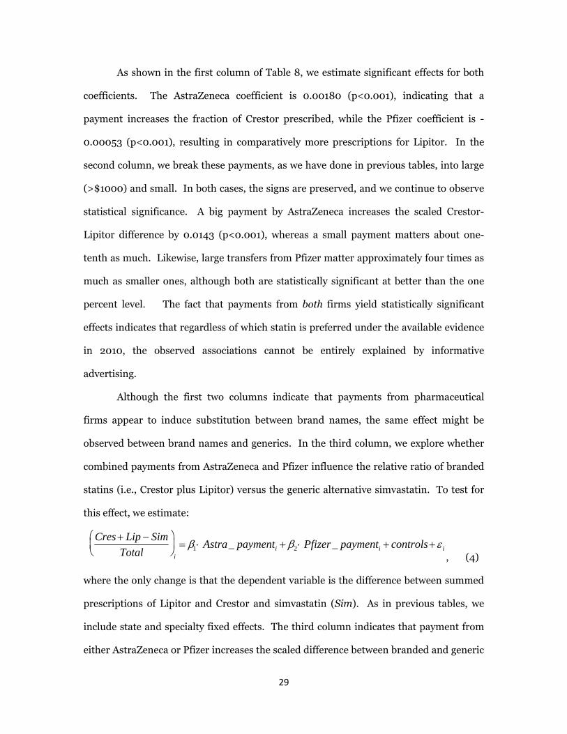
observed between brand names and generics. In the third column, we explore whether
combined payments from AstraZeneca and Pfizer influence the relative ratio of branded
statins (i.e., Crestor plus Lipitor) versus the generic alternative simvastatin. To test for
this effect, we estimate:
, (4)
where the only change is that the dependent variable is the difference between summed
prescriptions of Lipitor and Crestor and simvastatin (Sim). As in previous tables, we
include state and specialty fixed effects. The third column indicates that payment from
either AstraZeneca or Pfizer increases the scaled difference between branded and generic
Cres Lip Sim
Total
i
1 Astra_ paymenti 2 Pfizer_ paymenti controls i

30
statins. In the fourth and fifth columns, we break this up by firm, both of which are
shown to have a positive effect. In each case, large payments matter considerably more
than small payments.
To get a sense for the magnitude of wealth transfers in Table 8, we can use the
table’s coefficient estimates and the retail cost of statin drugs to estimate prescription
behavior with and without payment. This approach is conservative because it attributes
all of AstraZeneca’s and Pfizer’s payments to just these two drugs and only considers
doctors who wrote 50 or more prescriptions for the drugs. Nevertheless, in 2010 the
average retail cost of simvastatin (40 mg) was $68 while the cost for Crestor (40 mg) and
Lipitor (40 mg) were $162 and$165, respectively (Consumer Reports Health, 2010).7
Thus, the per-prescription cost difference between brand-names (taking the simple
average of Crestor and Lipitor costs) and generic simvastatin (assuming all 30-day
prescriptions and their equivalence to monthly costs) was $95.50.
Eliminating payments from Pfizer and AstraZeneca, i.e. setting the firms’
Payment Indicators to zero in the fourth column of Table 8, would have shifted
approximately 10 prescriptions per doctor, and 886,239 prescriptions in total, from
Crestor and Lipitor to simvastatin. According to this back-of-the-envelope exercise,
therefore, eliminating payment-induced brand-name prescriptions would have reduced
per-doctor expenditures by $955 and total expenditures by $84.64 million (changes in
firm revenue net of production costs would have likely been even higher). In 2011,
reported payments from AstraZeneca and Pfizer to providers totaled $308.48 million, so
a sizeable portion of total provider payments would have been returned from shifts in
prescriptions for just these two drugs among our sample of Medicare doctors. The per-
doctor expenditure shift is also worth several large meals or gifts.
7Averagecostsfor20mgdoseswereverysimilar,at$70(simvastatin),$164(Crestor),and$161(Lipitor).

31
Although drugs within the class of statins are plausible substitutes, they are not
chemically identical. Thus the possibility remains that the positive correlation between
payments and prescriptions for statins is driven by beliefs – rather than incentives – of
physicians. Put differently, although genuine information is unlikely to explain the
patterns observed in Table 8, doctors may nevertheless be persuaded by pharmaceutical
firms. The analysis in this section, because it considers identical chemicals, rules out
even uninformed persuasion.
We consider the case of drugs whose name-brand and generic equivalent are both
heavily prescribed in our 2010 sample. This is unusual, because insurance companies
rarely cover name-brand drugs which have available generic equivalents. In fact, we find
only five cases in which both a name-brand drug and its generic equivalent had at least
50 claims by at least 1,000 providers. Those drugs (and their generic equivalents) are
AstraZeneca’s Arimidex (anastrozole), Merck’s Cozaar (losartan potassium), Pfizer’s
Dilantin (phenytoin), GlaxoSmithKline’s Lanoxin (digoxin) and Pfizer’s Protonix
(pantoprazole). We remove Dilantin and Lanoxin from the analysis because of concerns
that the generic and name-brand are not chemically identical.8
We observe heavy volume for each of the three remaining drugs because of
changes in the drug’s exclusivity during 2010. Merck’s patent for high blood pressure
drug Cozaar expired in April (Doherty, 2010), and AstraZeneca’s patent for cancer drug
Arimidex expired in June (Connolly, 2010). In the case of Pfizer’s Protonix, generic
manufacturers were ordered by a US federal court in April to stop selling their generic
version of Pfizer’s drug due to patent infringement (Pearson et al., 2010). Patent
expiration and court orders are plausibly unrelated to a doctor’s belief about a drug’s
8Dilantinisanepilepsydrugwhoseusershavereportedincreasesinseizuresafterswitchingtogenericversions(http://www.webmd.com/epilepsy/news/20041025/generic‐epilepsy‐drugs‐not‐same),whileLanoxinhadwell‐publicizedrecallsofitsgenericequivalentbetween2008and2010(http://www.fda.gov/Safety/Recalls/ArchiveRecalls/ucm150734.htmandhttps://www.mediguard.org/alerts/alert/940.html).
32
efficacy. For this reason, these three drugs provide a natural setting for identifying the
incentive effects of payment behavior apart from beliefs.
While it is possible that a doctor might believe rosuvastatin (Crestor) to be more
effective than simvastatin, it seems unlikely that a doctor would believe any of our three
drugs are more effective than their generic twins. Thus any correlation we observe
between payments and the likelihood of prescribing the name brand in favor of the
generic is likely an effect of incentives, rather than beliefs.
We begin by considering the subset of doctors who prescribed either the name-
brand or the generic equivalent. For example, there were a total of 2,361 doctors who
prescribed the cancer drug Arimidex or its generic equivalent, anastrozole. For each of
these 2,361 doctors we create a binary variable called Name-Brand Indicator which
takes the value of one if a doctor prescribed the name brand drug in favor of the generic
equivalent (in the case where he prescribes both, a value of 1 is assigned to the drug with
the most prescriptions). Then we regress Name-Brand Indicator on Big Payment
Indicator and Small Payment Indicator in the first column of Table 9.
The positive coefficients on both Big Payment Indicator and Small Payment
Indicator demonstrate a positive relationship between payments from AstraZeneca and
prescriptions of Arimidex. Unconditionally, there is a 79% probability that name- brand
Arimidex is prescribed more frequently than its generic equivalent. However, this
probability increases to 81% if a doctor received a small payment from AstraZeneca and
to 98% if a doctor received a big payment from AstraZeneca. While the coefficient on
Small Payment Indicator is insignificant, the coefficient on Big Payment Indicator is
significant at the 1% level.
Columns 2 and 3 repeat the analysis for Merck’s Cozaar and Pfizer’s Protonix. In
the case of Cozaar we can only estimate a coefficient on Big Payment Indicator because
Merck reported only speaking fees (and not the less-lucrative meals and gifts) between

33
2009 and 2011 (see Table 1). The coefficient is positive but indistinguishable from zero.
In the case of Pfizer’s Protonix the coefficient of 0.116 on Big Payment Indicator
suggests that the probability of prescribing the name brand in favor of the generic
increases from 42.2% to 53.6% if a doctor received a big payment from Pfizer.
Column 4 combines the observations from the first three columns and finds that
the average increase in the probability of prescribing the name brand is 10.6% (p-value <
0.01) when Big Payment Indicator = 1. We find no effect for Small Payment Indicator.
The final column includes state and specialty fixed effects with little change in the
variables of interest.
In this special case, at least, it is worth emphasizing that the specialization
mechanism involves a realized financial conflict of interest, at worst, and a potentially
welfare-reducing oddity, at best: doctors with an idiosyncratic but demonstrably
incorrect belief in the branded drug are not only rewarded for their idiosyncrasy, but
their continued efforts at educating others about the branded drug could induce at least
some other physicians to make inappropriate prescriptions, however unlikely the
possibility.
B. Rent-seeking
The final explanation involves physicians altering their behavior in exchange for
current, or expected, financial benefits from pharmaceutical firms. Unlike the previous
alternatives involving information flow, this possibility is less capable of improving
decision making, and indeed, may worsen outcomes for patients. For example, financial
conflicts of interest may lead doctors to substitute a slightly inferior drug for another, or,
as seen in the last section, increase costs via reluctance to prescribe generic alternatives.
In this section, we develop two empirical proxies for the tendency for physicians
to engage in rent-seeking behavior. One is predominantly environmental, and the other
34
genetic. As we will see, both cut the data in the way that strongly suggests rent seeking
as an important determinant of the empirical patterns we observe.
The first source of variation is motivated by Glaeser and Saks’ (2006) study of
corruption across U.S. states. They use conviction rates for corruption-related crimes,
such as obstruction of justice, fraud, and election irregularities to proxy for state-level
rates of corruption. Our idea is that doctors living in more corrupt regions may,
themselves, be more sensitive to the payments of drug companies when making
prescription decisions.
In Figure 3, we plot the payment-prescription coefficient for each state on the y-
axis, as a function of Glaeser and Saks’ measure of political corruption on the x-axis,
shown as percentiles. States with low levels of corruption are shown toward the left, and
include Oregon (50th highest or 2nd percentile), Vermont (6th percentile), and Minnesota
(8th percentile). At the other end are high-corruption states: Illinois (88th percentile),
Louisiana (96% percentile), and Mississippi (98th percentile).
For each state, we run regression (2), using the same control variables (e.g.,
doctor specialty, pharmaceutical firm fixed effects, etc.) from Table 5, Panel B. The
coefficient of interest is on the Any_payment dummy variable, interpreted as the
additional prescriptions the typical doctor prescribes for a given drug company’s
products, conditional on him receiving a payment from that company. Because states
vary so widely in the number of doctors, we scale each point estimate by the standard
error of the estimated coefficient, so that a circle with twice the diameter of another is
estimated twice as precisely.
Visual inspection reveals an upward sloping relation between prescription
sensitivities to payments across states and convictions for corruption related crimes. Of
the ten least corrupt states, eight have estimated sensitivities below 20, with only three
states below the median corruption level exceeding 25. On the other hand, almost two-

35
thirds of states above the median are associated with coefficients above 25, with seven
exceeding 35. Interestingly, the one notable outlier, Alaska, is associated with the
highest per-capita conviction rate, and also the only negative estimated prescription-
payment sensitivity. However, with only 253 Alaskan doctors entering the estimation,
this is not statistically significant.
In Table 10, we formalize these comparisons in regressions. The first three
columns show the results of estimating Equation (2) by corruption tercile, progressing
from least to most corrupt. Confirming the graphical evidence shown in Figure 3, the
first column indicates a point estimate of 20.2 prescriptions (p<0.001) for the least
corrupt third of U.S. states. The coefficient increases by almost half in the second
column to 28.3 (p<0.001), and yet again for the most corrupt states (30.91, p<0.001).
The fourth column aggregates all states together, and interacts the numerical value of the
Glaeser-Saks corruption index percentiles, the same numbers displayed the x-axis of
Figure 3. The t-statistic on the interaction is negative seven, indicating a steeply
declining impact for drug company payments in less corrupt states.
In light of these findings, it is worth examining the heat maps shown in Figure 4.
Note that both payments and prescription rate of branded drugs are heavily
concentrated in the greater southeast region of the U.S. Focusing on Panel B, note that
gulf coast states Texas, Louisiana, Mississippi, Alabama, and Florida, as well as
neighbors Georgia and South Carolina – all above median rates of corruption – have
significantly elevated prescription rates of branded drugs. States with high branded
rates in different regions include New York (7th most corrupt state), New Jersey (17th),
and Alaska (1st).
Combining all three pictures, a theme emerges: doctors in corrupt states are most
sensitive to payments (Figure 3), pharmaceuticals disproportionately target these

36
regions (Figure 4A), and the distribution of branded drugs reflects the combination of
these effects (Figure 4B).
What these graphical patterns cannot tell us, however, is why – i.e., what is it
about certain regions that fosters corrupt activity across very different areas, ranging
from corrupt elected officials to rent seeking physicians? Manski’s (1993) discussion of
the “reflection problem” in social effects provides a useful context. Endogenous effects
refer to classic “peer effects,” such as a teenager going to the beach because (and only
because) her friends are also going. Exogenous effects refer to common characteristics
that lead groups to behave similarly, e.g., a group of fair-skinned avoiding the beach
together for common fear of sunburn. Correlated effects refer to operating under a
common environment, such as news of a shark attack inducing a “correlated” response
by those living nearby.
Any of these seem plausible in our setting, and we cannot convincingly
distinguish between them. For example, there are considerable demographic differences
between states, some of which reflect exogenous attributes, and others which reflect
common environmental influences. Poverty and education rates also differ considerably
between states, both of which are positively related to corruption (Berkowitz and Clay,
2004). There is also the possibility that corruption reflects social norms, being more
tolerated in some regions than in others. This latter possibility corresponds to an
endogenous effect, and is capable of explaining how corruption in two different arenas –
i.e., politics and medicine – could be so strongly correlated within regions.
The only mechanism that probably can be excluded is cross-state differences in
enforcement, a contextual factor often making causal inferences in corruption studies
difficult. Two features of our setting make this less problematic. The first is a feature of
Glaeser and Saks’ measure of corruption itself. As the authors note, all convictions were
prosecuted by the Federal Department of Justice, rather than local jurisdictions. Second,

37
even were this not the case, receiving payments from drug companies is, in the vast
majority of circumstances, not illegal, making its enforcement (or lack of enforcement)
largely irrelevant.
The second cross-sectional proxy we use is physician gender. Studies of political
corruption have found an inverse relationship between participation rates of females in
government and political corruption (Dollar et al., 2001; Swamy et al., 2001). As with
state-level variation, we explore whether groups (here defined by gender) more likely to
exhibit corruption in one arena are more likely to manifest it in another.
To investigate this issue, we use the database of Cong et al. (2011) which collects
first names and self-identified genders from Facebook. For example, if an individual’s
first name is “Daniel” that person self-identifies as male 99.7% of the time, but if an
individual’s first name is “Stephanie” that person self-identifies as male 0.04% of the
time. Some names are more ambiguous, such as “Blake” (87.4% male), “Pat” (45.8%
male) and “Morgan” (39.8% male). From the database we create a Male dummy variable
which takes the value one if the probability of male is at least 90% and takes the value of
zero if the probability of male is less than 10%. For the ambiguous names (between 10%
and 90%) the Male variable is assigned a missing value. According to this classification
scheme, 71.7% of the doctors in our sample are male.
The fifth and sixth columns indicate that male doctors are almost twice as
sensitive to industry payments (30.51) as female physicians (17.73). The next column
aggregates both males and females into a single specification, with the final column
adding an interaction for state-level corruption; both coefficients remain highly
significant.
We view the gender result as useful for both specific and general reasons.
Specifically, it helps to better identify the mechanism underlying the pay-prescription
relation observed in our sample of physicians. Whereas it makes little sense to think that

38
information flow between firms and doctors would differ across males and female
physicians, studies from other settings (e.g., politics) suggest that gender differences in
corruption should be expected. Further, the fact that this result survives, and indeed
appears almost independent of, the effect of state-level corruption, lends further support
to the idea that rent seeking by physicians is at least part of the story.
More generally, whether women appear to engage in less corruption (in any
setting) is itself subject to multiple interpretations. For example, does this reflect
differences in exogenous characteristics, such as an inherent distaste for corruption or
dishonesty? Or, are institutional or contextual effects – such as women paying a higher
price for getting caught – a more plausible explanation? While difficult to make these
distinctions in studies of political corruption, the fact that tilting prescriptions toward
friendly drug companies is neither illegal nor enforced suggests that the patterns
observed likely reflect inherent differences in attitudes toward corruption between the
sexes.
VI. Conclusion
Using data from twelve drug companies, more than 330,000 physicians and
nearly one billion prescriptions, we find that when a drug company pays a doctor he is
more likely to prescribe that company’s drug. Our specifications are stringent,
accounting for pharmaceutical firm, state, specialty, and even physician-firm match
effects. Rent-seeking behavior on the part of doctors appears to be an important
consideration, as evidenced by a higher payment-prescription relation in states ranking
high in corruption.
Whether these results are surprising likely depends on whether one views a
physician – and her opinions – as sacrosanct. To a cynical reader, perhaps the presence
of influence is self-evident from payments: after all, if payments from firms to doctors

39
did not change doctor behavior, why would profit-maximizing firms choose to make
them in the first place? While this view seems sensible from an economist’s perspective,
it ignores the fact that payments may reflect (rather than cause) the opinions of
physicians or represent valuable transfers of information from firms to doctors. Given
that the balance of our evidence is best explained by either persuasive advertising from
drug companies or rent-seeking behavior from doctors, to a less-cynical reader our
findings suggest a consideration of outside influences when taking in medical advice.
In the same way, our results have clear policy implications. If payment behavior
simply reflects a doctor’s already-held opinion, then mandatory disclosure of physician
payments (as required by the 2014 Physician Payment Sunshine Act) would impose an
unnecessary cost on the healthcare system. Instead, given our evidence that payments
incentivize or persuade doctors to change their behavior, disclosure of these transfers
will help patients to best interpret and understand the medical advice they receive.

40
References
American College of Physicians. Physicians and the Pharmaceutical Industry. Annals of Internal Medicine 1990; 112; 624–626. http://dx.doi.org/10.7326/0003-4819-112-8-624.
Berkowitz D, Clay K. Initial conditions, institutional dynamics and economic performance: Evidence from the American states. 615. 2004.
Centers for Medicare & Medicaid Services. 2013. Medicare, Medicaid, Children’s Health Insurance Programs; Transparency Reports and Reporting of Physician Ownership or Investment Interests. 2013. Available at: https://www.federalregister.gov/articles/2013/02/08/2013-02572/transparency-reports-and-reporting-of-physician-ownership-or-investment-interests-medicare-medicaid.
Connolly A. AstraZeneca Profit Fell on Generic Rivals, Legal Costs. Bloomberg.com. October 28, 2010.
Consumer Reports Health. 2010. Evaluating statin drugs to treat: High Cholesterol and Heart Disease. 2010. Available at: http://www.tcyh.org/admin/images/doc_uploads/BBD-Statins-2pg.pdf.
Coyle SL. Physician–Industry Relations. Part 1: Individual Physicians. Annals of Internal Medicine 2002; 136; 396–402. http://dx.doi.org/10.7326/0003-4819-136-5-200203050-00014.
Dave DM. Effects of Pharmaceutical Promotion: A Review and Assessment. National Bureau of Economic Research Working Paper Series 2013; No. 18830. http://www.nber.org/papers/w18830.
Doherty D. Novartis Profit Climbs on Pandemic Flu Vaccine Sales. Bloomberg.com. April 20, 2010.
Dollar D, Fisman R, Gatti R. Are women really the “fairer” sex? Corruption and women in government. Journal of Economic Behavior & Organization 2001; 46; 423–429. http://www.sciencedirect.com/science/article/pii/S016726810100169X.
Endo A. The origin of the statins. Atherosclerosis Supplements 2004; 5; 125–130. http://www.sciencedirect.com/science/article/pii/S1567568804000728.
Glaeser EL, Saks RE. Corruption in America. Journal of Public Economics 2006; 90; 1053–1072. http://www.sciencedirect.com/science/article/pii/S004727270500126X.
Gottlieb DJ, Zhou W, Song Y, Andrews KG, Skinner JS, Sutherland JM. Prices Don’t Drive Regional Medicare Spending Variations. Health Affairs 2010; 29 537–543. http://content.healthaffairs.org/content/29/3/537.abstract.

41
Heyes A. The economics of vocation or “why is a badly paid nurse a good nurse”? Journal of Health Economics 2005; 24; 561–569. http://www.sciencedirect.com/science/article/pii/S0167629604001043.
Istvan ES, Deisenhofer J. Structural Mechanism for Statin Inhibition of HMG-CoA Reductase. Science 2001; 292 1160–1164. http://www.sciencemag.org/content/292/5519/1160.abstract.
Jones PH, Davidson MH, Stein EA, Bays HE, McKenney JM, Miller E, Cain VA, Blasetto JW. Comparison of the efficacy and safety of rosuvastatin versus atorvastatin, simvastatin, and pravastatin across doses (STELLAR Trial). The American Journal of Cardiology 2003; 92; 152–160. http://www.sciencedirect.com/science/article/pii/S0002914903005307.
Katz D, Caplan AL, Merz JF. All Gifts Large and Small: Toward an Understanding of the Ethics of Pharmaceutical Industry Gift-Giving. The American Journal of Bioethics 2010; 10; 11–17. http://dx.doi.org/10.1080/15265161.2010.519226.
Larkin, Ian, Desmond Ang, Matthew Chao, and Tina Wu. 2012. “The Impact of Pharmaceutical Detailing on Physician Prescribing: Quasi-Experimental Evidence from Academic Medical Center Policy Changes”. Cambridge, MA.
Luvai A, Mbagaya W, Hall AS, Barth JH. Rosuvastatin: A Review of the Pharmacology and Clinical Effectiveness in Cardiovascular Disease. Clinical Medicine Insights: Cardiology 2012; 6; 17–33. www.la-press.com/rosuvastatin-a-review-of-the-pharmacology-and-clinical-effectiveness-i-article-a3036.
Madhavan S, Amonkar MM, Elliott D, Burke K, Gore P. The gift relationship between pharmaceutical companies and physicians: an exploratory survey of physicians. Journal of Clinical Pharmacy and Therapeutics 1997; 22; 207–218. http://dx.doi.org/10.1046/j.1365-2710.1997.94975949.x.
Manski CF. Identification of Endogenous Social Effects: The Reflection Problem. The Review of Economic Studies 1993; 60 531–542. http://restud.oxfordjournals.org/content/60/3/531.abstract.
Medicare Payment Advisory Committee. 2009. Public reporting of physicians’ financial relationships, Chapter 5 in Report to the Congress: Medicare payment policy. Washington, DC; 2009. Available at: http://www.medpac.gov/documents/mar09_entirereport.pdf.
Mullahy J. Much ado about two: reconsidering retransformation and the two-part model in health econometrics. Journal of Health Economics 1998; 17; 247–281. http://www.sciencedirect.com/science/article/pii/S0167629698000307.
Nicholls SJ, Ballantyne CM, Barter PJ, Chapman MJ, Erbel RM, Libby P, Raichlen JS, et al. Effect of Two Intensive Statin Regimens on Progression of Coronary Disease. New England Journal of Medicine 2011; 365; 2078–2087. http://dx.doi.org/10.1056/NEJMoa1110874.

42
Nicholls SJ, Brandrup-Wognsen G, Palmer M, Barter PJ. Meta-analysis of Comparative Efficacy of Increasing Dose of Atorvastatin Versus Rosuvastatin Versus Simvastatin on Lowering Levels of Atherogenic Lipids (from VOYAGER). The American Journal of Cardiology 2010; 105; 69–76. http://www.sciencedirect.com/science/article/pii/S0002914909022164.
Pearson S, Decker S, Voreacos D. Pfizer Reaches $2.15 Billion Protonix Accord With Teva. Bloomberg.com. June 12, 2010.
Pham-Kanter, G, G Alexander, and K Nair. 2012. “Effect of Physician Payment Disclosure Laws on Prescribing.” Archives of Internal Medicine 172 (10) (May 28): 819–821. http://dx.doi.org/10.1001/archinternmed.2012.1210.
ProPublica. 2013a. Dollars for Doctors: How Industry Money Reaches Physicians. 2013. Available at: http://www.propublica.org/series/dollars-for-docs.
———. 2013b. Prescriber Checkup: The Doctors and Drugs in Medicare Part D. 2013. Available at: http://projects.propublica.org/checkup/.
Rebitzer JB, Taylor LJ. 2011. Chapter 8 - Extrinsic Rewards and Intrinsic Motives: Standard and Behavioral Approaches to Agency and Labor Markets. In: Economics OA and DCBT-H of L (Ed), vol. Volume 4, Elsevier; 2011. pp. 701–772.
Swamy A, Knack S, Lee Y, Azfar O. Gender and corruption. Journal of Development Economics 2001; 64; 25–55. http://www.sciencedirect.com/science/article/pii/S0304387800001231.
Tang C, Ross K, Saxena N, Chen R. 2011. What’s in a Name: A Study of Names, Gender Inference, and Gender Behavior in Facebook. In: Xu J, Yu G, Zhou S, Unland R (Ed). Database Systems for Adanced Applications SE - 33, vol. 6637. Springer Berlin Heidelberg; 2011. pp. 344–356.
U.S. Bureau of Labor Statistics. 2010. Occupational Outlook Handbook: Physicians and Surgeons. 2010. Available at: http://www.census.gov/hhes/www/cpstables/032011/perinc/new01_001.htm.
U.S. Census Bureau. 2010. Current Population Survey Annual Social and Economic Supplement. 2010. Available at: http://www.census.gov/hhes/www/cpstables/032011/perinc/new01_001.htm.
Wazana A. Physicians and the pharmaceutical industry: Is a gift ever just a gift? JAMA 2000; 283; 373–380. http://dx.doi.org/10.1001/jama.283.3.373.

43
Figure 1: Payments and Prescriptions per Patient
The top panel plots prescriptions per patient for drugs of our twelve pharmaceutical firms. The bottom panel plots prescriptions per patient for drugs not from our twelve pharmaceutical firms. In both panels, doctors are first sorted into decile bins according to total prescriptions and then into decile bins according to total payments from our twelve pharmaceutical firms.
PANEL A: Prescriptions per Patient for Pharmaceutical Firm Drugs
PANEL B: Prescriptions per Patient for non-Pharmaceutical Firm Drugs
0
0.5
1
1.5
2
2.5
3
3.5
NotPaid
PaidtheLeast
PaidtheMost
FewestPrescriptions
MostPrescriptions
0
5
10
15
20
25
30
NotPaid
PaidtheLeast
PaidtheMost
FewestPrescriptions
MostPrescriptions

44
Figure 2: Payments and Headquarter Geography
The graph plots the mean payment from pharmaceutical firms to physicians by location. Closest (farthest) physicians are those within 100 (500) kilometers of pharmaceutical headquarters.
$‐
$50.00
$100.00
$150.00
$200.00
$250.00
$300.00
$350.00
$400.00
$450.00
100KM(Closest)
200KM 300KM 400KM 500KM(Furthest)
AveragePharmaPayment
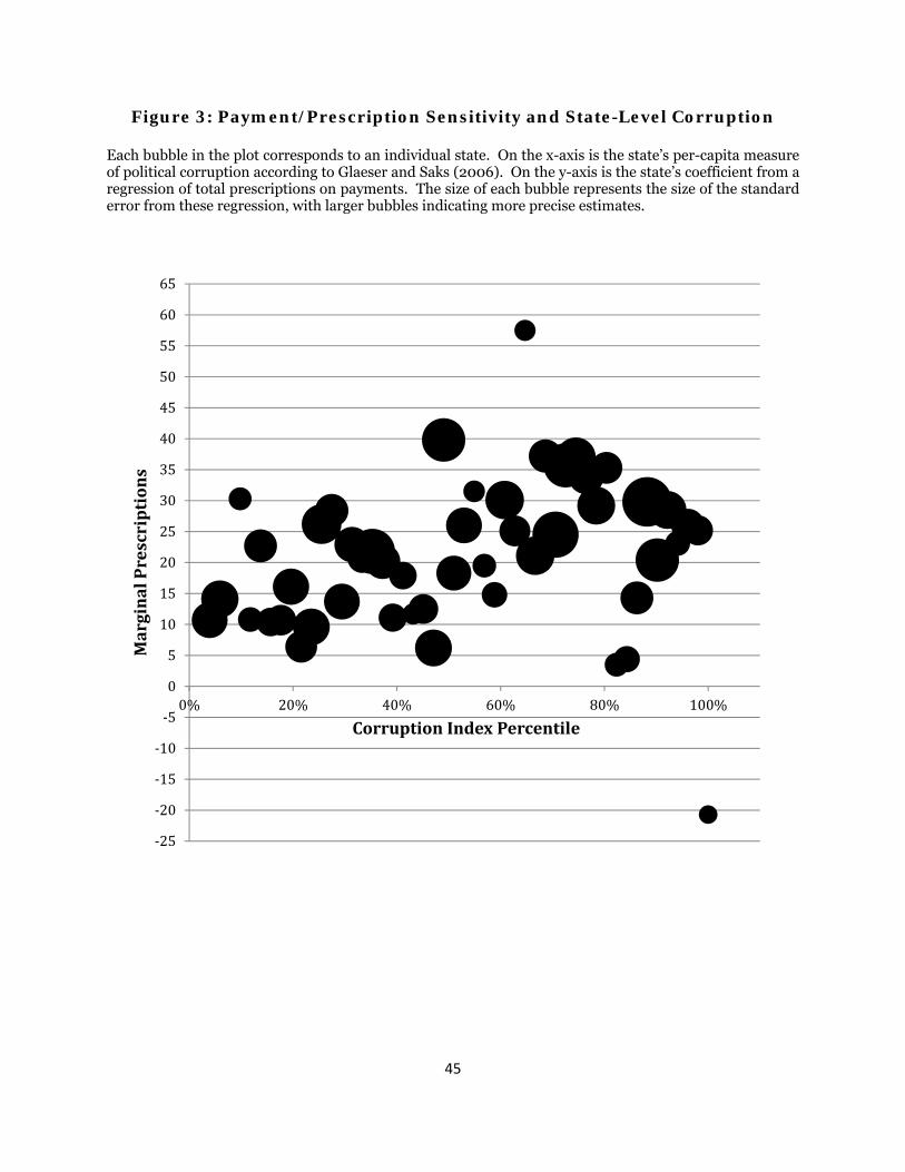
45
Figure 3: Payment/Prescription Sensitivity and State-Level Corruption
Each bubble in the plot corresponds to an individual state. On the x-axis is the state’s per-capita measure of political corruption according to Glaeser and Saks (2006). On the y-axis is the state’s coefficient from a regression of total prescriptions on payments. The size of each bubble represents the size of the standard error from these regression, with larger bubbles indicating more precise estimates.
‐25
‐20
‐15
‐10
‐5
0
5
10
15
20
25
30
35
40
45
50
55
60
65
0% 20% 40% 60% 80% 100%
MarginalPrescriptions
CorruptionIndexPercentile
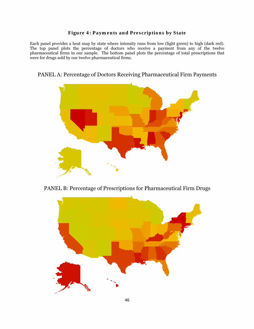
46
Figure 4: Payments and Prescriptions by State
Each panel provides a heat map by state where intensity runs from low (light green) to high (dark red). The top panel plots the percentage of doctors who receive a payment from any of the twelve pharmaceutical firms in our sample. The bottom panel plots the percentage of total prescriptions that were for drugs sold by our twelve pharmaceutical firms.
PANEL A: Percentage of Doctors Receiving Pharmaceutical Firm Payments
PANEL B: Percentage of Prescriptions for Pharmaceutical Firm Drugs

47
Table 1: Payments and Reporting Practices by Pharmaceutical Firms
The top panel describes the reporting practice for payments to healthcare providers by each of twelve pharmaceutical firms during the period 2009 - 2011. Data are taken from ProPublica’s Dollars for Docs database (ProPublica 2013a). Reporting varies by year and categories reported. The top panel also includes the number of unique providers to whom payment was made as well as total dollars paid by year. The bottom panel provides summary statistics for the various payment categories.

48
PANEL A: Pharmaceutical Firms and Reporting Practices 2009 2010 2011
Categories Providers Total $
Reported Categories Providers Total $
Reported Categories Providers Total $
Reported
Allergan - - - None Identified 41,528 - Research, Gifts, Meals, Royalties, Speaking, Travel
42,572 -
AstraZeneca - - - Speaking 2,381 $31.47M Consulting, Gifts, Meals, Research, Speaking, Travel
116,643 $114.21M
Cephalon None Identified 935 $9.25M Consulting, Gifts, Meals, Research, Speaking, Travel
45,575 $21.00M Consulting, Gifts, Meals, Research, Speaking, Travel
36,157 $31.17M
Eli Lilly Consulting, Speaking, Other 4,963 $82.09M
Consulting, Speaking, Travel,
Other 4,875 $77.75M
Consulting, Meals, Research,
Speaking, Travel, Other
101,898 $226.40M
EMD Serono - - - - - - Consulting, Gifts, Meals, Speaking,
Travel, Other 11,112 $1.85M
GlaxoSmithKline Consulting, Speaking 5,716 $50.60M Consulting,
Speaking 5,249 $56.76M Consulting, Research, Speaking
4,909 $120.82M
Johnson & Johnson
- - -
Combination, Consulting, Meals, Speaking, Travel,
Other
2,166 $17.94M Consulting, Meals, Speaking, Travel,
Other 80,704 $22.96M
Merck Speaking 1,640 $9.29M Speaking 2,019 $20.00M Speaking 2,454 $26.50M
Novartis - - - - - - Speaking 3,259 $24.58M
Pfizer Consulting, Gifts, Meals, Research, Speaking, Travel
4,738 $37.63M Consulting, Gifts, Meals, Research, Speaking, Travel
196,453 $176.70M Consulting, Gifts, Meals, Research, Speaking, Travel
161,025 $194.27M
Valeant - - - Consulting, Gifts, Meals, Other 6,136 $306.69K
Consulting, Expenses, Gifts, Meals, Speaking,
Travel, Other
15,855 $1.50M
Viiv - - - Consulting, Research, Speaking
435 $7.84M Consulting, Research, Speaking
524 $8.79M
All Pharmas 16,096 $188.86M 264,137 $409.78M 388,451 $773.05M

49
PANEL B: Payment Size by Type
Observations Mean Standard Deviation
5th Percentile
25th Percentile Median
75th Percentile
95th Percentile
Consulting 20,940 $4,205 $10,300 $75 $700 $2,000 $4,000 $13,647
Gifts/Items 102,423 $80 $580 $9 $45 $72 $99 $169
Meals 1,295,221 $74 $125 $11 $16 $37 $93 $239
Research 20,961 $51,262 $226,724 $675 $4,650 $14,631 $44,257 $183,550
Speaking 65,238 $9,969 $16,634 $700 $2,000 $4,500 $10,651 $41,900
Travel 34,849 $1,312 $2,647 $20 $104 $565 $1,294 $5,499
Other 90,991 $313 $2,461 $10 $12 $23 $58 $257

50
Table 2: Sample Summary Statistics The table provides summary statistics by doctor in Panel A and by (Doctor, Firm) pair in Panel B. The set of doctors and Medicare Part D claims are taken from the ProPublica Prescriber Checkup database (ProPublica 2013b). Total payments are the sum of all payments between 2009 and 2011 from the ProPublica Dollars for Docs database (ProPublica 2013a). “Branded” claims are insurance claims for drugs marketed by our twelve pharmaceutical firms.
PANEL A: By Doctor
Observations Mean Standard Deviation
5th Percentile
25th Percentile
Median 75th
Percentile 95th
Percentile
Total Payments 334,086 $2,108 $25,870 $0 $0 $14 $146 $1,701
Payment Indicator 334,086 0.58 0.49 0 0 1 1 1
Total Patients 334,086 217 177.18 51 105 174 280 519
Total Medicare Claims 334,086 2980 4,061 213 637 1,527 3,710 10,508
Total Branded Medicare Claims 334,086 192 439 0 0 55 203 851
Total Patients | Payment Indicator = 1 192,484 243 175 61 123 200 314 564
Total Medicare Claims | Payment Indicator = 1 192,484 3566 4,521 302 850 1,954 4,552 12,099
Total Branded Medicare Claims | Payment Indicator = 1 192,484 258 519 0 0 84 299 1,059
PANEL B: By (Doctor, Firm) Pair
Observations Mean Standard Deviation
5th Percentile
25th Percentile Median 75th
Percentile 95th
Percentile
Payment Indicator 4,009,032 0.11 0.31 0 0 0 0 1
Payment Size | Payment Indicator = 1 398,772 $1,766 $21,403 $11 $23 $57 $143 $3,378
Prescription Indicator 4,009,032 0.10 0.30 0 0 0 0 1
Prescriptions | Prescription Indicator = 1 398,515 161 183 52 65 102 185 451

51
Table 3: Payments and Prescription Rates for Physicians The dependent variable is prescriptions per patient for drugs of our twelve pharmaceutical firms. Log(Total Payments) is the natural logarithm of total payments between 2009 and 2011 from our twelve pharmaceutical firms. Residual Firm Prescriptions per Patient are the prescriptions per patient for drugs not from our twelve pharmaceutical firms. Paid Zero Indicator is a binary variable which takes the value of one if a doctor was not paid. Paid Decile = X Indicator is a binary variable which takes the value of one is a doctor is in decile X of the payment distribution. Robust standard errors are in parentheses. *, **, and *** represent significance at the 10%, 5% and 1% levels, respectively.
Dependent Variable: Pharmaceutical Firm Prescriptions per Patient
Log(Total Payments) 0.0865*** 0.0733*** 0.0702*** (0.00137) (0.00139) (0.00137) Residual Prescriptions per Patient 0.0722*** 0.0919*** 0.0918*** (0.000529) (0.000797) (0.000799) Paid Zero Indicator -0.151*** -0.156*** -0.150*** (0.00705) (0.00653) (0.00653) Paid Decile = 1 Indicator -0.112*** -0.0810*** -0.0722*** (0.00876) (0.00799) (0.00792) Paid Decile = 2 Indicator -0.0917*** -0.0690*** -0.0645*** (0.00888) (0.00813) (0.00806) Paid Decile = 3 Indicator -0.0699*** -0.0464*** -0.0482*** (0.00925) (0.00848) (0.00842) Paid Decile = 4 Indicator -0.0710*** -0.0441*** -0.0436*** (0.00898) (0.00825) (0.00817) Paid Decile = 6 Indicator 0.0412*** 0.0415*** 0.0395*** (0.00980) (0.00898) (0.00889) Paid Decile = 7 Indicator 0.0798*** 0.0829*** 0.0798*** (0.00987) (0.00910) (0.00900) Paid Decile = 8 Indicator 0.168*** 0.169*** 0.163*** (0.0104) (0.00964) (0.00955) Paid Decile = 9 Indicator 0.300*** 0.295*** 0.280*** (0.0113) (0.0106) (0.0106) Paid Decile = 10 Indicator 0.516*** 0.412*** 0.407*** (0.0123) (0.0119) (0.0118) Specialty Fixed Effects NO YES YES NO YES YES State Fixed Effects NO NO YES NO NO YES Non-Pharma 12 Decile Fixed Effects NO NO NO YES YES YES Observations 179,432 179,432 179,432 334,086 334,086 334,086 Adjusted R2 0.319 0.425 0.437 0.275 0.381 0.390
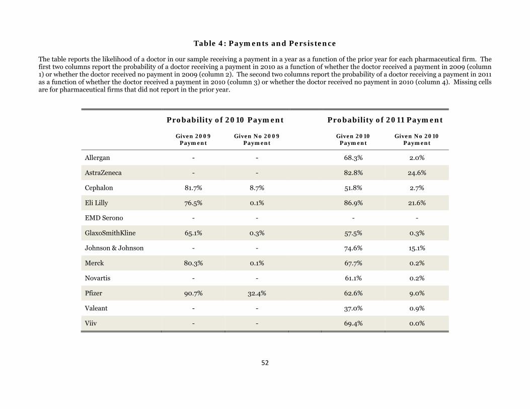
52
Table 4: Payments and Persistence The table reports the likelihood of a doctor in our sample receiving a payment in a year as a function of the prior year for each pharmaceutical firm. The first two columns report the probability of a doctor receiving a payment in 2010 as a function of whether the doctor received a payment in 2009 (column 1) or whether the doctor received no payment in 2009 (column 2). The second two columns report the probability of a doctor receiving a payment in 2011 as a function of whether the doctor received a payment in 2010 (column 3) or whether the doctor received no payment in 2010 (column 4). Missing cells are for pharmaceutical firms that did not report in the prior year.
Probability of 2010 Payment Probability of 2011 Payment
Given 2009 Payment
Given No 2009 Payment Given 2010
Payment Given No 2010
Payment
Allergan - - 68.3% 2.0%
AstraZeneca - - 82.8% 24.6%
Cephalon 81.7% 8.7% 51.8% 2.7%
Eli Lilly 76.5% 0.1% 86.9% 21.6%
EMD Serono - - - -
GlaxoSmithKline 65.1% 0.3% 57.5% 0.3%
Johnson & Johnson - - 74.6% 15.1%
Merck 80.3% 0.1% 67.7% 0.2%
Novartis - - 61.1% 0.2%
Pfizer 90.7% 32.4% 62.6% 9.0%
Valeant - - 37.0% 0.9%
Viiv - - 69.4% 0.0%

53
Table 5: Payments and Prescription Behavior for (Doctor, Firm) Pairs The table relates payments made by pharmaceutical firms to prescribing behavior. The unit of observation is a (Doctor, Firm) pair. The dependent variable in the top panel, Prescription Indicator, is binary and equals one if the doctor prescribes any of the pharmaceutical firm’s drugs at least 50 times. The dependent variable in the bottom panel is total prescriptions. Robust standard errors are in parentheses. *, **, and *** represent significance at the 10%, 5% and 1% levels, respectively. PANEL A
Dependent Variable: Prescription Dummy Log Payments 2009 0.0274***
(0.000500) Payment 2009 Dummy 0.227***
(0.00433) Log Payments 2010 0.0281***
(0.000249) Payment 2010 Dummy 0.156***
(0.00112) Log Payments 2011 0.0269***
(0.000177) Payment 2011 Dummy 0.129***
(0.000725) Log Total Payments 0.0270***
(0.000156) Any Payment Dummy 0.126***
(0.000674) Any Payment - Big 0.207*** 0.207*** 0.209***
(0.00277) (0.00277) (0.00288) Any Payment - Small 0.0946*** 0.0893*** 0.0906***
(0.000697) (0.000712) (0.00074) Total Prescriptions 3.16e-05*** 3.16e-05*** 2.74e-05*** 2.50e-05*** 2.45e-05*** 2.25e-05*** 2.24e-05*** 2.25e-05*** 2.45e-05***
(1.60e-07) (1.60e-07) (1.04e-07) (9.11e-08) (9.13e-08) (8.11e-08) (8.11e-08) (8.10e-08) (9.14e-08)
State Fixed Effects YES YES YES YES YES YES YES YES YES - - Specialty Fixed Effects YES YES YES YES YES YES YES YES YES - - Pharma Fixed Effects YES YES YES YES YES YES YES YES YES YES - Doctor Fixed Effects NO NO NO NO NO NO NO NO NO YES YES Pharma-Zip Fixed Effects NO NO NO NO NO NO NO NO NO NO YES Observations 1,670,430 1,670,430 3,340,860 3,674,946 3,674,945 4,009,032 4,009,032 4,009,032 3,674,946 3,674,946 3,674,946 Adjusted R2 0.321 0.320 0.300 0.287 0.299 0.287 0.288 0.288 0.299 0.308 0.315

54
PANEL B
Dependent Variable: Total Prescriptions
Log Payments 2009 6.947*** (0.196)
Payment 2009 Dummy 58.30*** (1.708)
Log Payments 2010 8.327*** (0.100)
Payment 2010 Dummy 43.47*** (0.424)
Log Payments 2011 6.201*** (0.0602)
Payment 2011 Dummy 28.89*** (0.236)
Log Total Payments 6.375*** (0.0542)
Any Payment Dummy 27.86*** (0.211)
Any Payment - Big 59.69*** 58.50*** 58.60*** (1.223) (1.116) (1.280)
Any Payment - Small 18.84*** 21.00*** 20.67*** (0.194) (0.196) (0.214)
Total Prescriptions 0.0112*** 0.0112*** 0.00932*** 0.00852*** 0.00838*** 0.00773*** 0.00770*** 0.00772*** 0.00840*** (0.000113) (0.000113) (6.99e-05) (6.49e-05) (6.50e-05) (6.06e-05) (6.04e-05) (6.06e-05) (6.51e-05)
State Fixed Effects YES YES YES YES YES YES YES YES YES - - Specialty Fixed Effects YES YES YES YES YES YES YES YES YES - - Pharma Fixed Effects YES YES YES YES YES YES YES YES YES YES - Doctor Fixed Effects NO NO NO NO NO NO NO NO NO YES YES Pharma-Zip Fixed Effects NO NO NO NO NO NO NO NO NO NO YES Observations 1,670,430 1,670,430 3,340,860 3,674,946 3,674,945 4,009,032 4,009,032 4,009,032 3,674,946 3,674,946 3,674,946 Adjusted R2 0.324 0.324 0.297 0.263 0.282 0.251 0.252 0.251 0.281 0.3670 0.3778

55
Table 6: Specialization
Only Meal Payment Indicator takes the value of one for a (Doctor, Firm) pair if a doctor only received a meal as payment from a pharmaceutical firm. Columns 1 and 2 repeat the analysis of Panel A of Table 5 (Column 10) but restrict attention to only the drugs outside a doctor’s top five and top ten most prescribed drugs. Robust standard errors are in parentheses. *, **, and *** represent significance at the 10%, 5% and 1% levels, respectively.
Dependent Variable: Total Prescriptions
Outside Top 5 Outside Top 10
Any Payment Indicator - Big 37.28*** 29.23*** (1.126) (1.144) Any Payment Indicator - Small 15.23*** 11.92*** (0.232) (0.247) Only Meal Payment Indicator 22.86*** (0.205) Pharma Fixed Effects YES YES YES Doctor Fixed Effects NO NO NO Observations 1,940,444 1,393,227 2,279,173 Adjusted R2 0.343 0.355 0.256

56
Table 7: Quasi-exogenous transfers to physicians inferred from geography The table shows the same specification from Table 5B, except that payments are instrumented using the distance (in km) from each doctor’s office to the relevant pharmaceutical firm. The unit of observation is a (Doctor, Firm) pair. Sample is limited to doctor-firm pairs within 500 km. The dependent variable is the total number of prescriptions written by doctor i for drugs marketed by firm j. Robust standard errors are in parentheses. *, **, and *** represent significance at the 10%, 5% and 1% levels, respectively.
Dependent Variable: Total Prescriptions
Any Payment – Small (instrumented) 189.5*** 99.72***
(24.54) (10.94)
Any Payment – Big (instrumented) 991.6*** 729.1***
(160.9) (98.80)
Any Payment (instrumented) 176.5*** 106.4***
(21.22) (10.80)
Total Prescriptions 0.00639*** 0.00868*** 0.00612***
(0.000336) (6.81e-05) (0.000264)
State Fixed Effects YES - YES - YES -
Specialty Fixed Effects YES - YES - YES -
Pharma Fixed Effects YES YES YES YES YES YES
Doctor Fixed Effects NO YES NO YES NO YES
Number of Observations 422,343 360,315 422,343 360,315 446,675 360,315
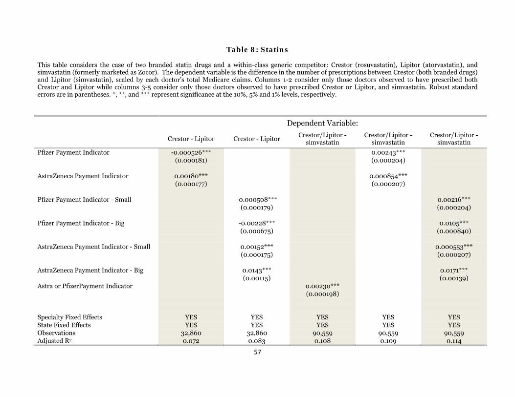
57
Table 8: Statins
This table considers the case of two branded statin drugs and a within-class generic competitor: Crestor (rosuvastatin), Lipitor (atorvastatin), and simvastatin (formerly marketed as Zocor). The dependent variable is the difference in the number of prescriptions between Crestor (both branded drugs) and Lipitor (simvastatin), scaled by each doctor’s total Medicare claims. Columns 1-2 consider only those doctors observed to have prescribed both Crestor and Lipitor while columns 3-5 consider only those doctors observed to have prescribed Crestor or Lipitor, and simvastatin. Robust standard errors are in parentheses. *, **, and *** represent significance at the 10%, 5% and 1% levels, respectively.
Dependent Variable:
Crestor - Lipitor Crestor - Lipitor
Crestor/Lipitor - simvastatin
Crestor/Lipitor - simvastatin
Crestor/Lipitor - simvastatin
Pfizer Payment Indicator -0.000526*** 0.00243*** (0.000181) (0.000204) AstraZeneca Payment Indicator 0.00180*** 0.000854*** (0.000177) (0.000207) Pfizer Payment Indicator - Small -0.000508*** 0.00216*** (0.000179) (0.000204) Pfizer Payment Indicator - Big -0.00228*** 0.0105*** (0.000675) (0.000840) AstraZeneca Payment Indicator - Small 0.00152*** 0.000553*** (0.000175) (0.000207) AstraZeneca Payment Indicator - Big 0.0143*** 0.0171*** (0.00115) (0.00139) Astra or PfizerPayment Indicator 0.00230*** (0.000198) Specialty Fixed Effects YES YES YES YES YES State Fixed Effects YES YES YES YES YES Observations 32,860 32,860 90,559 90,559 90,559 Adjusted R2 0.072 0.083 0.108 0.109 0.114

58
Table 9: Name-Brand vs. Generic Drugs This table considers the case of three name-brand drugs and their generic equivalents: Arimidex (anastrozole), Cozaar (losartan potassium) and Protonix (pantoprazole). The dependent variable, Name-Brand Indicator, is a binary variable that takes the value of 1 if a doctor prescribes the name-brand instead of the generic (in the case where she prescribes both, a value of 1 is assigned to the drug with the most prescriptions). Column 1 (2, 3) considers only the set of doctors who prescribed Arimidex (Cozaar, Protonix) or its generic equivalent. Columns 4 and 5 combine all of the observations in the first three columns. Robust standard errors are in parentheses. *, **, and *** represent significance at the 10%, 5% and 1% levels, respectively.
Dependent Variable: Name-Brand Indicator
Arimidex Cozaar Protonix All All
Payment Indicator - Big 0.190*** 0.0273 0.116*** 0.107*** 0.0853***
(0.00847) (0.0307) (0.0283) (0.0233) (0.0207)
Payment Indicator - Small 0.0217 -0.00757 -0.00345 0.00809
(0.0173) (0.00847) (0.00767) (0.00698)
Firm Fixed Effects NO NO NO YES YES Specialty Fixed Effects NO NO NO NO YES
State Fixed Effects NO NO NO NO YES
Observations 2,361 12,707 12,477 27,545 27,545
Adjusted R2 0.002 0.000 0.001 0.294 0.400

59
Table 10: Rent-Seeking The dependent variable is the total number of prescriptions in the (Doctor, Firm) pair. Columns 1 (2, 3) consider the subset of states in the bottom (middle, top) tercile of the Glaeser and Saks (2006) corruption index. Columns 5 (6) consider the subset of doctors which have a male (female) first name. Robust standard errors are in parentheses. *, **, and *** represent significance at the 10%, 5% and 1% levels, respectively.
Dependent Variable: Total Prescriptions | Prescription Indicator = 1
Low Corruption
States
Medium Corruption
States
High Corruption
States All Males Females All All
Any Payment Indicator 20.17*** 28.26*** 30.91*** 17.71*** 30.51*** 17.73*** 12.53*** 2.664***
(0.352) (0.376) (0.336) (0.434) (0.261) (0.397) (0.399) (0.558)
Any Payment Indicator * Corruption Index 0.183*** 0.181***
(0.00739) (0.00780)
Male -3.325*** -3.296***
(0.0869) (0.0871)
Any Payment Indicator * Male 19.40*** 19.19***
(0.469) (0.470)
Total Prescriptions 0.00668*** 0.00888*** 0.00741*** 0.00772*** 0.00765*** 0.00714*** 0.00753*** 0.00753***
(0.000176) (0.000119) (6.81e-05) (6.06e-05) (7.26e-05) (0.000157) (6.53e-05) (6.54e-05)
Specialty Fixed Effects YES YES YES YES YES YES YES YES
State Fixed Effects YES YES YES YES YES YES YES YES
Pharma Fixed Effects YES YES YES YES YES YES YES YES
Observations 989,112 1,371,588 1,648,332 4,000,608 2,497,248 985,956 3,483,204 3,476,196
Adjusted R2 0.255 0.243 0.263 0.252 0.263 0.210 0.252 0.253
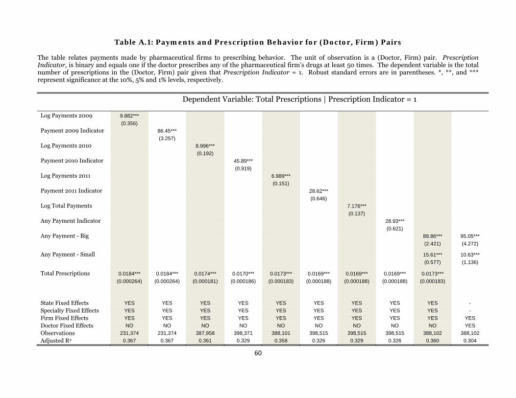
60
Table A.1: Payments and Prescription Behavior for (Doctor, Firm) Pairs The table relates payments made by pharmaceutical firms to prescribing behavior. The unit of observation is a (Doctor, Firm) pair. Prescription Indicator, is binary and equals one if the doctor prescribes any of the pharmaceutical firm’s drugs at least 50 times. The dependent variable is the total number of prescriptions in the (Doctor, Firm) pair given that Prescription Indicator = 1. Robust standard errors are in parentheses. *, **, and *** represent significance at the 10%, 5% and 1% levels, respectively.
Dependent Variable: Total Prescriptions | Prescription Indicator = 1
Log Payments 2009 9.882*** (0.356) Payment 2009 Indicator 86.45*** (3.257) Log Payments 2010 8.996*** (0.192) Payment 2010 Indicator 45.89*** (0.919) Log Payments 2011 6.989*** (0.151) Payment 2011 Indicator 28.62*** (0.646) Log Total Payments 7.176*** (0.137) Any Payment Indicator 28.93*** (0.621) Any Payment - Big 89.86*** 95.05*** (2.421) (4.272)
Any Payment - Small 15.61*** 10.63*** (0.577) (1.136)
Total Prescriptions 0.0184*** 0.0184*** 0.0174*** 0.0170*** 0.0173*** 0.0169*** 0.0169*** 0.0169*** 0.0173*** (0.000264) (0.000264) (0.000181) (0.000186) (0.000183) (0.000188) (0.000188) (0.000188) (0.000183) State Fixed Effects YES YES YES YES YES YES YES YES YES - Specialty Fixed Effects YES YES YES YES YES YES YES YES YES - Firm Fixed Effects YES YES YES YES YES YES YES YES YES YES Doctor Fixed Effects NO NO NO NO NO NO NO NO NO YES Observations 231,374 231,374 387,958 398,371 388,101 398,515 398,515 398,515 388,102 388,102 Adjusted R2 0.367 0.367 0.361 0.329 0.358 0.326 0.329 0.326 0.360 0.304

61


