DETERMINATION OF SUBGRADE STRENGTH UNDER
INTACT PORTLAND CEMENT CONCRETE SLABS FORRUBBLIZATION PROJECTS
Final Report(Report No. FHWA/NC/2002-010)
To North Carolina Department of Transportation(Research Project No. HWY-1999-02)
Submitted by
Y. Richard Kim, Ph.D., P.E.Campus Box 7908
Department of Civil EngineeringNorth Carolina State University
Raleigh, NC 27695-7908Ph: 919-515-7758Fax: 919-515-7908
E-mail: [email protected]
Sungho MunGraduate Student
May 2002

Technical Report Documentation Page
1. Report No.FHWA/NC/2002-010
2. Government Accession No.
3. Recipient’s Catalog No.
4. Title and SubtitleDetermination of Subgrade Strength under Intact Cement Concrete Slabsfor Rubblization Projects
5. Report DateMay 21, 2002
6. Performing Organization Code
7. Author(s)Y. Richard Kim and Sungho Mun
8. Performing Organization Report No.
9. Performing Organization Name and Address 10. Work Unit No. (TRAIS)North Carolina State UniversityDepartment of Civil EngineeringCampus Box 7908Raleigh, NC 27695-7908
11. Contract or Grant No.
12. Sponsoring Agency Name and AddressNorth Carolina Department of TransportationResearch and Analysis Group1 South Wilmington StreetRaleigh, NC 27601
13. Type of Report and Period CoveredFinal ReportJuly 1998 - June 2000
14. Sponsoring Agency Code1999-02
15. Supplementary Notes
16. AbstractRubblization is an effective rehabilitation method for deteriorated Portland cement concrete (PCC) pavements due to its low
initial cost, minimum traffic disruption, and ability to minimize reflective cracking in asphalt overlays. However, the loss ofstrength in PCC slab due to rubblization creates the demand for a subgrade that is strong enough to handle traffic afterrubblization. AASHTO recommends Falling Weight Deflectometer (FWD) testing of PCC pavements before rubblization toascertain the subgrade strength after rubblization. However, the existing deflection analysis methods do not adequately handle thechange in stress states in the subgrade before and after rubblization, and therefore result in erroneous prediction of subgradestrength. The primary objective of this study is to develop an analysis method that allows the realistic estimation of subgradestrength after rubblization from deflection measurements on intact PCC slabs before rubblization. As a forward model,stress/strain dependent nonlinear subgrade models were incorporated into a finite element analysis. ABAQUS and NCPAVE, afinite element code developed at North Carolina State University, were used in the analysis. Multi-load FWD testing wasconducted in the field to generate varying stress states in the subgrade under intact PCC pavements. Based on the syntheticdatabase generated from the finite element analyses, a number of relationships were developed using regression and ArtificialNeural Network (ANN) approaches to predict the coefficients in the nonlinear subgrade model from multi-load FWD deflections.The verification study was performed on the resulting algorithms using limited field data derived from US 29 in Guilford Countyand I-85 in Rowan County. The research suggests that the stress-based regression approach, which determines the nonlinearcoefficients by regressing between the subgrade moduli and stresses predicted at several radial distances from the FWD loadfrom multi-load deflections, is the most promising method of analysis. The research team strongly recommends the furtherverification of this procedure using additional field data before the implementation.
17. Key WordsRubblization, Subgrade Strength, Falling Weight
Deflectometer, PCC Pavement, Multi-Load FWD,Nonlinear Behavior of Subgrade
18. Distribution Statement
19. Security Classif. (of this report)Unclassified
20. Security Classif. (of this page)Unclassified
21. No. of Pages115
22. Price
Form DOT F 1700.7 (8-72) Reproduction of completed page authorized
i
ABSTRACT
Rubblization is an effective rehabilitation method for deteriorated Portland
cement concrete (PCC) pavements due to its low initial cost, minimum traffic disruption,
and ability to minimize reflective cracking in asphalt overlays. However, the loss of
strength in PCC slab due to rubblization creates the demand for a subgrade that is strong
enough to handle traffic after rubblization. AASHTO recommends Falling Weight
Deflectometer (FWD) testing of PCC pavements before rubblization to ascertain the
subgrade strength after rubblization. However, the existing deflection analysis methods
do not adequately handle the change in stress states in the subgrade before and after
rubblization, and therefore result in erroneous prediction of subgrade strength.
The primary objective of this study is to develop an analysis method that allows the
realistic estimation of subgrade strength after rubblization from deflection measurements
on intact PCC slabs before rubblization. As a forward model, stress/strain dependent
nonlinear subgrade models were incorporated into a finite element analysis. ABAQUS
and NCPAVE, a finite element code developed at North Carolina State University, were
used in the analysis. Multi-load FWD testing was conducted in the field to generate
varying stress states in the subgrade under intact PCC pavements. Based on the synthetic
database generated from the finite element analyses, a number of relationships were
developed using regression and Artificial Neural Network (ANN) approaches to predict
the coefficients in the nonlinear subgrade model from multi-load FWD deflections. The
verification study was performed on the resulting algorithms using limited field data
derived from US 29 in Guilford County and I-85 in Rowan County. The research
suggests that the stress-based regression approach, which determines the nonlinear

ii
coefficients by regressing between the subgrade moduli and stresses predicted at several
radial distances from the FWD load from multi-load deflections, is the most promising
method of analysis. The research team strongly recommends the further verification of
this procedure using additional field data before the implementation.

iii
DISCLAIMER
The contents of this report reflect the views of the authors and not necessarily the views
of the University. The authors are responsible for the facts and the accuracy of the data
presented herein. The contents do not necessarily reflect the official views or policies of
either the North Carolina Department of Transportation or the Federal Highway
Administration at the time of publication. This report does not constitute a standard,
specification, or regulation.

iv
ACKNOWLEDGMENTS
The authors would like to acknowledge the support of the North Carolina Department of
Transportation and the Federal Highway Administration. Special thanks go to engineers
in the Pavement Management Unit for their help in FWD testing.

v
TABLE OF CONTENTS
LIST OF TABLES............................................................................................................ vii
LIST OF FIGURES ........................................................................................................... ix
1. INTRODUCTION ......................................................................................................... 1
1.1 Research Objective and Report Organization .......................................................... 4
1.2 Rubblization in North Carolina ................................................................................ 5
2. LITERATURE REVIEW ............................................................................................ 11
2.1 PCC Rehabilitation Techniques.............................................................................. 11
2.1.1 Saw and Seal .................................................................................................... 11
2.1.2 Crack/Seat and Break/Seat ............................................................................... 12
2.1.3 Rubblization ..................................................................................................... 12
2.2 Stress-State Dependent Subgrade Models.............................................................. 14
2.2.1 Granular Soil .................................................................................................... 15
2.2.2 Fine-Grained Soil ............................................................................................. 18
2.3 Strain-Dependent Subgrade Model ........................................................................ 20
3. PCC PAVEMENT ANALYSIS .................................................................................. 23
3.1 FEM Program ......................................................................................................... 24
3.2 Nonlinearity Using FWD Multi-Level Loads ........................................................ 25
3.3 Forward Model ....................................................................................................... 26
3.4 Dynamic vs. Static Analysis................................................................................... 32
4. SUBGRADE CONDITION PREDICTION ALGORITHMS USING ANN.............. 36
4.1 Stress-Based ANN Model for General Soils .......................................................... 37
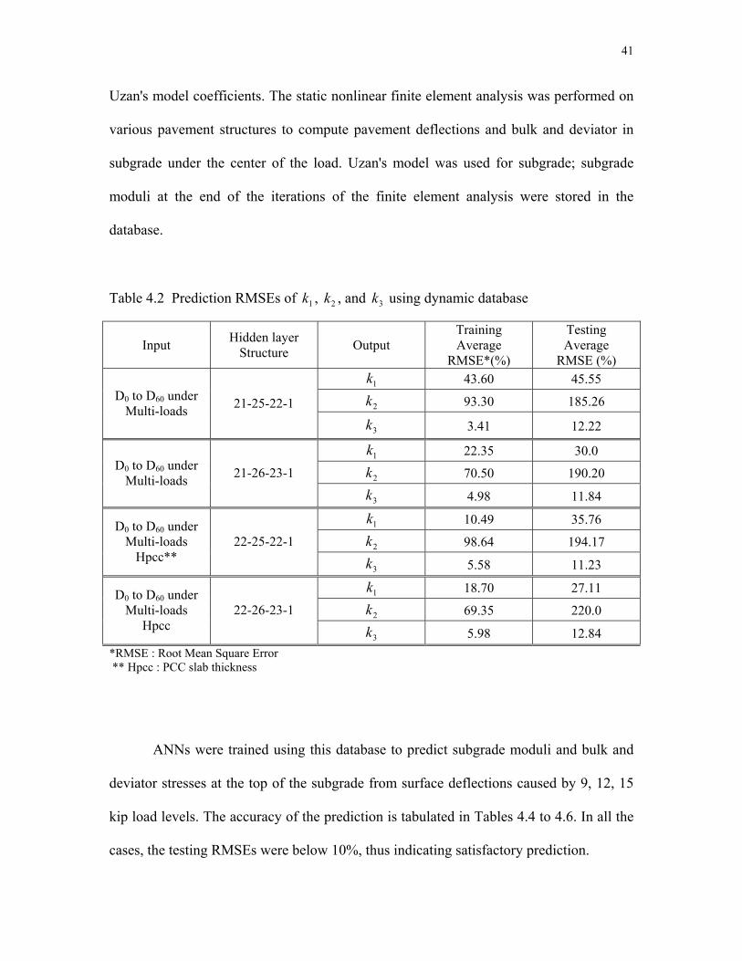
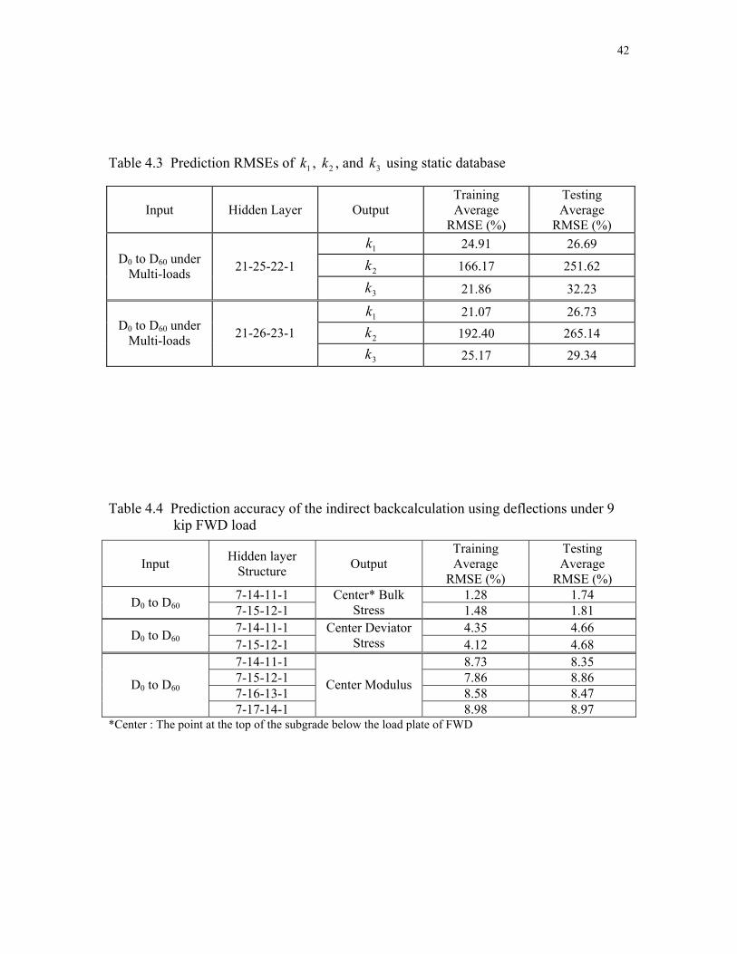
4.1.1 Direct Backcalculation ..................................................................................... 40
4.1.2 Regression Approach Using ANN Backcalculated Stresses and Moduli ........ 40
4.2 Stress-Based ANN Model for Cohesive Soils........................................................ 44
4.2.1 Direct Backcalculation for Cohesive Soils....................................................... 46
4.2.2 Regression Approach for Cohesive Soils......................................................... 47
4.3 Strain-Based ANN Model for Cohesive Soils........................................................ 51

vi
4.3.1 Backcalculation Using ANN............................................................................ 53
5. PERFORMACE EVALUATION OF DEVELOPED PROCEDURES ...................... 56
5.1 In -Situ FWD Database........................................................................................... 56
5.1.1 Highway US 29 ................................................................................................ 56
5.1.2 Interstate Highway I-85.................................................................................... 57
5.2 Deflection Basin Parameter .................................................................................... 60
5.3 Prediction of Subgrade Nonlinearity Using Field FWD Deflections ..................... 61
5.4 Comparison between Measured and Calculated Deflections ................................. 69
5.5 Recommended Procedure ....................................................................................... 79
6. CONCLUSIONS AND RECOMMENDATIONS FOR FUTURE RESEARCH....... 80
6.1 Conclusions ............................................................................................................ 80
6.2 Recommendations .................................................................................................. 81
LIST OF REFERENCES.................................................................................................. 82
APPENDIX A. ESTIMATION OF LAYER CONDITION............................................ 88
A.1 Existing Backcalculation Methods for Rigid Pavement........................................ 89
A.1.1 Theoretical Models for Backcalculation ......................................................... 89
A.1.1.1 Hertz-Westerggard Model......................................................................... 89
A.1.1.2 Hogg Model............................................................................................... 90
A.1.1.3 Multi-layered Elastic Model...................................................................... 91
A.2.1 Backcalculation Procedures ............................................................................ 91
A.2.1.1 JUSLAB Procedures.................................................................................. 91
A.2.1.2 ILLI-BACK Procedures ............................................................................ 92
A.2.1.3 RMODS Program...................................................................................... 96
A.3 Base Damage Index and Shape Factor F2 ............................................................. 96
A.4 Artificial Neural Networks .................................................................................... 98
A.5 Genetic Algorithm Optimization Technique ....................................................... 101

vii
LIST OF TABLES
2.1 Resilient modulus models for granular materials ....................................................... 19
2.2 Resilient modulus models for cohesive soils .............................................................. 20
3.1 Ranges of material properties in intact PCC slab and subgrade ................................. 32
4.1 The ranges of the input variables for forward modeling............................................. 37
4.2 Prediction RMSEs of , , and k using dynamic database.................................. 41 1k 2k 3
4.3 Prediction RMSEs of , , and k using static database ....................................... 42 1k 2k 3
4.4 Prediction accuracy of the indirect backcalculation using deflections under 9 kip
FWD load .................................................................................................................. 42
4.5 Prediction accuracy of the indirect backcalculation using deflections under 12 kip
FWD load .................................................................................................................. 43
4.6 Prediction accuracy of the indirect backcalculation using deflections under 15 kip
FWD load .................................................................................................................. 43
4.7 Material properties and thicknesses used in ABAQUS FEM.................................... 45
4.8 Prediction accuracy of the direct backcalculation using different input units under
multi FWD loads ....................................................................................................... 46
4.9 Prediction RMSEs of deviator stresses on top of subgrade using the calculated D0 to
D60 deflections based on ABAQUS dynamic FEM .................................................. 48
4.10 Prediction RMSEs of moduli on top of subgrade using the calculated D0 to D60
deflections based on ABAQUS dynamic FEM......................................................... 49
4.11 Prediction accuracy of the regression approach........................................................ 49
4.12 Prediction RMSEs of stresses on top of subgrade using the calculated D0 to D24
deflections based on ABAQUS dynamic FEM......................................................... 49
4.13 Prediction RMSEs of moduli on top of subgrade using the calculated D0 to D24
deflections based on ABAQUS dynamic FEM......................................................... 50
4.14 Prediction accuracy using the calculated D0 to D24 deflections according to ANN
structure ..................................................................................................................... 51
viii
4.15 Ranges of the input variables to be used in forward modeling for the strain-based
approach ................................................................................................................... 53
4.16 Prediction RMSEs of strains and moduli at the top of subgrade using the calculated
D0 to D24 deflections.................................................................................................. 54
5.1 Layer information and locations in the tested pavement ........................................... 56
5.2 Prediction accuracy of the direct backcalculation using different input units under 9
kip and 12 kip FWD loads......................................................................................... 65
5.3 Nonlinear model prediction using 9 and 12 kip load deflections of I-85 FWD tests 66
5.4 Predicted PCC moduli for the four locations on I-85 ................................................ 67
ix
LIST OF FIGURES
2.1 Resonant frequency breaker....................................................................................... 13
2.2 Rubblized concrete by resonant frequency breaker ................................................... 14
2.3 Principal stresses on a finite soil element .................................................................. 16
2.4 Variation in normalized Young’s modulus with PI value ......................................... 21
3.1 Normalized deflection vs. load level: (a) center deflection and (b) seventh deflection
database ................................................................................................................. 28
3.2 Degree of nonlinearity from US 29 FWD tests [(D0 under 15kip – D0 under 9kip)/D0
under 9kip] ............................................................................................................... 29
3.3 Normalized load used for dynamic analysis .............................................................. 30
3.4 Infinite element model of a pavement system ........................................................... 30
3.5 Sensor spacing and FWD testing configuration......................................................... 31
3.6 Transient deflections calculated by ABAQUS dynamic analysis.............................. 31
3.7 Deflection plots (a) thin structure, strong PCC and strong subgrade; (b) thin
structure, weak PCC and strong subgrade; (c) thin structure, strong PCC and weak
subgrade; and (d) thin structure, weak PCC and weak subgrade .............................. 34
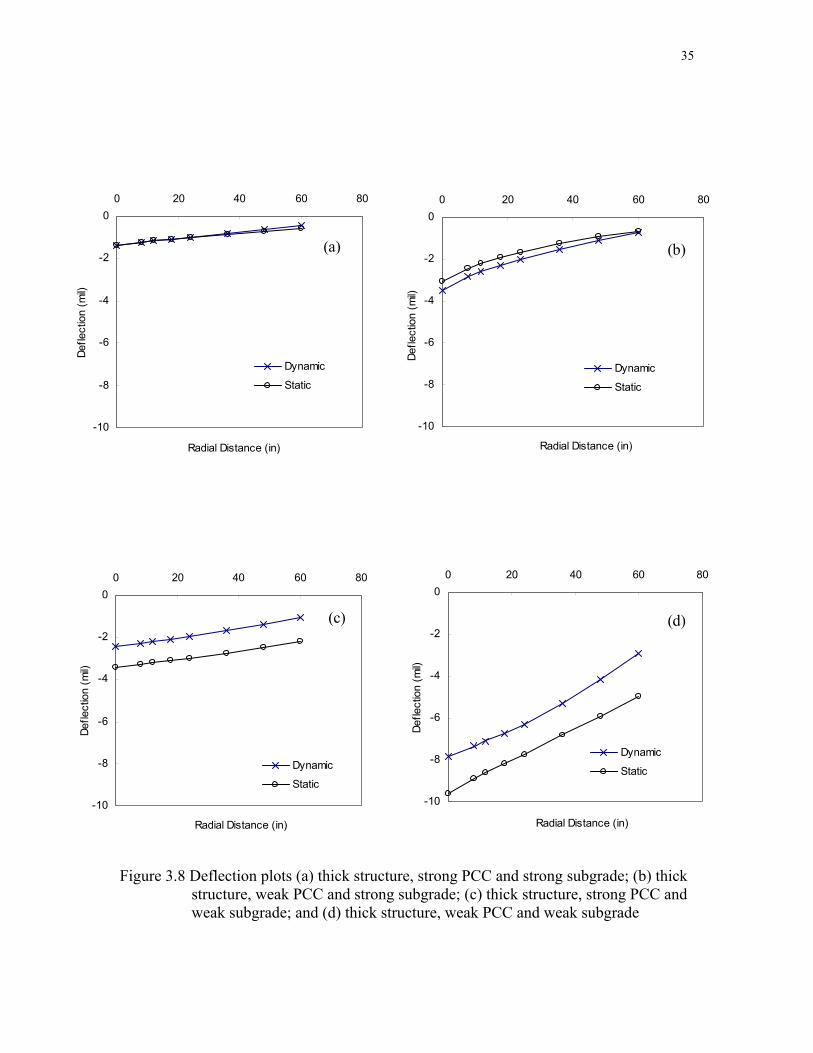
3.8 Deflection plots (a) thick structure, strong PCC and strong subgrade; (b) thick
structure, weak PCC and strong subgrade; (c) thick structure, strong PCC and weak
subgrade; and (d) thick structure, weak PCC and weak subgrade ............................ 35
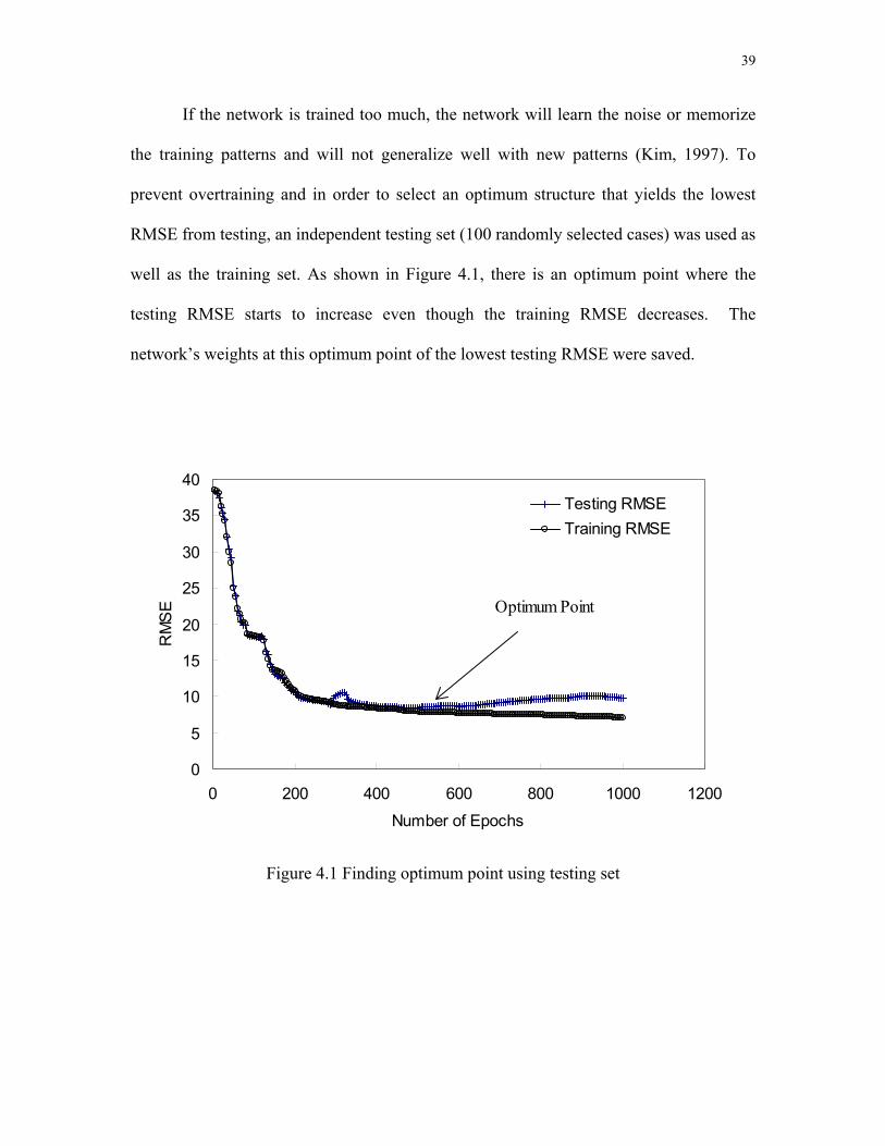
4.1 Finding optimum point using testing set.................................................................... 39
4.2 Locations of calculated deflections, deviator stresses, and moduli ........................... 45
4.3 Two examples of the regression approach................................................................. 47
4.4 Prediction of Uzan’s coefficients (a) and (b) ................................................... 52 1k 3k
4.5 Variation in normalized Young's modulus vs. axial strain (From Kim, 1992) ......... 55
4.6 Comparison between selected curve and curves obtained from lab tests using NC
soils ........................................................................................................................... 55

x
5.1 Deflection profiles for US 29 before rubblization: (a) D0 and (b) D60 ...................... 59
5.2 FWD deflections at station 216 on US 29 ................................................................ 60
5.3 BDI vs. F2: (a) under 9 kips; (b) under 12 kips; and (c) under 15 kips .................... 62
5.4 Predicted vs. actual PCC modulus ............................................................................ 67
5.5 Linear regression plots from backcalculated deviator stresses and moduli............... 68
5.6 CBR vs. depth from surface at loaction A ................................................................. 70
5.7 The linear relationship curve between DCP reading and CBR.................................. 71
5.8 Comparison plot under 3 kip FWD load on bare base test ........................................ 72
5.9 Comparison plot under 5 kip FWD load on bare base test ........................................ 73
5.10 Comparison plot under 7 kip FWD load on bare base test ...................................... 74
5.11 Absolute errors between calculated and measured deflections under 3 kip FWD load
on bare base ............................................................................................................... 76
5.12 Absolute errors between calculated and measured deflections under 5 kip FWD load
on bare base .............................................................................................................. 76
5.13 Absolute errors between calculated and measured deflections under 7 kip FWD load
on bare base ............................................................................................................... 77
5.14 Absolute errors between calculated and measured deflections under 9 kip FWD load
on intact PCC slabs.................................................................................................... 77
5.15 Absolute errors between calculated and measured deflections under 12 kip FWD
load on intact PCC slabs............................................................................................ 78
A.1 Variation of AREA with l (Ioannides, 1994)............................................................ 93
A.2 Characteristic trends between F2 and BDI for identifying subgrade stiffness
independent of upper layer condition........................................................................ 97
A.3 Biological and neural networks................................................................................. 99
A.4 Typical multilayered network with one hidden layer and output layer .................. 100
A.5 Genetic algorithm cycle .......................................................................................... 102
A.6 Schematic diagram of genetic algorithm techniques .............................................. 104

1
CHAPTER ONE INTRODUCTION
According to the National Asphalt Pavement Association (NAPA), there are
approximately 500,000 lane miles of Portland cement concrete (PCC) pavement within
the United States highway system (PCS, 1991). About one-half of these pavements
comprise the current Interstate System. There are many techniques currently used to
rehabilitate these aging PCC pavements. The majority of the techniques commonly used
today incorporate either an asphalt concrete (AC) or PCC overlay. Among the most
popular is a simple surface course overlay using hot-mix asphalt to restore surface
rideability and integrity. The major problem of AC overlay over PCC slabs is the
recurrence of cracks in the rehabilitated surface layer, known as reflective cracking. In
order to retard the reflective cracking, one may think that an overlay thickness may be
increased. However, according to Corley-Lay (1995), Indiana DOT reported “thicker
overlays increased construction costs but did not reduce long term reflective cracking.”
Several rehabilitation techniques have been developed to deal with reflective
cracking in overlays on PCC pavement (refer to Chapter 2). Since the late 80's, a new
technique called rubblization has received increasing attention as a viable solution to
minimize reflective cracking in overlays on PCC pavement. The technique involves
destroying the existing PCC slab into pieces smaller than one foot in order to provide an
improved base material for the future overlay. In this manner, the deteriorated PCC
pavement is essentially converted to a high-strength granular base and gives the
appearance of an unbound base material as in AC pavement construction.
2
According to the NAPA report (PCS, 1991), rubblization is most suitable for
cases where PCC slabs have deteriorated to a point where there is little potential of
significant slab integrity or structural capacity using other rehabilitative techniques. They
add, however, that rubblizing appears to be equally effective for all types of PCC
pavement types and that it is actually the preferred method when any type of slab
reinforcement is present. A preliminary investigation for the Wisconsin Department of
Transportation (Nelson and Owusu-Ababio, 1994) concluded, “rubblization techniques
have been successfully used on PCC pavements exhibiting punchouts, delaminations,
patching, and cracking in both the longitudinal and transverse directions.”
Given the relatively short time period since the rubblization was first introduced
in 1986 (Schackner, 1989), there is not a very strong database of information to
adequately gauge the performance of the rubblized sections. However, preliminary
investigations tend to indicate that the vast majority of the rubblized pavements are
performing well with respect to reflection crack control, rideability, etc. Also, the
rubblization technique results in lower initial cost and minimum disruption of traffic and
safety-related problems due to accelerated construction.
NCDOT also had success in the first rubblization project on I-95 in Northhampton
County. Since then, NCDOT has used the rubblization technique in several major
projects, including I-440 beltline around Raleigh, I-85 North of Durham, and NC-26 near
Beulahville. However, the experience of NCDOT in these rubblized projects results in a
mixed feeling due to inaccurate estimation of subgrade strength before rubblization (refer
to Section 1.2).

3
For the rubblization project to be successful, it is important to have a subgrade
that is strong enough to handle the traffic after the PCC layer loses its strength due to
rubblization. AASHTO recommends deflection testing of the pavement (ASTM D 4694
and D 4695) in order to better ascertain its structural properties (AASHTO, 1993). This
testing is normally accomplished using a heavy-load deflection device such as a Falling
Weight Deflector (FWD) and measuring the pavement response in terms of deflection.
The FWD tests provide some insight into the structural capacity of the pavement and base
layer(s) or subgrade before rehabilitation. If the results of the deflection tests prove to be
unsatisfactory or, if the tests are not used at all, AASHTO recommends coring and
material testing of the deteriorated pavement. It is also recommended that deflection tests
be performed on the fractured slabs after rubblization to confirm the structural capacity of
the resultant structure. To date, there is no accepted method to directly correlate pre- and
post-rubblization moduli of subgrade.
The NCDOT has experienced significant differences in backcalculated moduli on
a recent project on I-85 North of Durham (Corley-Lay, 1997). The effect of this
variability in backcalculated moduli for rubblized sections can be potentially very costly
and timely. For example, if a certain subgrade is believed to be stronger than post-
rubblization tests reveal, it may be necessary to abort rubblization, undercut the rubblized
sections and proceed with a full-depth pavement design and construction. DOTs,
contractors, and taxpayers are obviously very eager to be able to ascertain the condition
of the pavement structure before rehabilitation contracts are let out for bid.

4
Rubblization as a rehabilitative technique has continually proved to be an
effective method for managing aged and deteriorated PCC pavements due to appealing
performance and the recent advancements in equipment technology. To fully take
advantage of this technique, North Carolina Department of Transportation has funded a
two-year research project “Determination of Subgrade Strength under Intact Portland
Cement Concrete Slabs for Rubblization Projects.” This report presents the findings from
the project and the recommended procedure for estimating subgrade modulus under
rubblized PCC slabs from FWD deflections measured on PCC pavements prior to
rubblization.
1.1 Research Objective and Report Organization
The primary objective of this research is to develop an analysis method that
enables the estimation of subgrade modulus after rubblization from deflection
measurements on intact PCC slabs before rubblization. To accomplish this objective,
nonlinear behavior of subgrade under multi-level FWD loads was investigated using
finite element analysis. Several backcalculation (or so-called inversion) algorithms were
evaluated as the vehicle to predict the subgrade condition from measured deflections.
Findings from this research will be presented in seven chapters in this report, and the
brief description of each chapter is given below.
Chapter 2 presents a literature review on the rehabilitation techniques of PCC
pavements and nonlinear models of subgrade. The understanding of nonlinear behavior of
subgrade soils is essential for predicting post-rubblization subgrade moduli from
deflections measured from PCC slabs before rubblization. Both stress and strain based

5
nonlinear models are presented. Chapter 3 introduces the finite element analysis used in
this study to incorporate the nonlinear model of subgrade. Chapter 4 presents the details
involved in developing several subgrade condition evaluation algorithms. These
algorithms are evaluated in Chapter 5 using limited field data, and the recommendation is
made based on the comparison of their performance. Chapter 6 provides the conclusions
of the study as well as future research direction in this research area. Various
backcalculation algorithms for subgrade modulus are briefly summarized in Appendix A.
1.2 Rubblization in North Carolina
Since its inception, rubblization has been used on many projects throughout the
United States. A brief discussion of some rubblized projects across the nation is given
below, followed by case studies in North Carolina.
The first known project to use rubblization was Route 146 in Clifton Park, NY
around 1986 (Schackner, 1989). The Route 146 project was a two-mile stretch which
was to be used as a test program for the larger, upcoming Route 7 project. The result of
using rubblization cut the project price tag in half along with increasing the expected
design life of the roadway. In 1990, an eight to nine inch concrete pavement was
rubblized on I-59 in Laurel, MS with appreciable success (Kuennen, 1991). During the
same year, a section of I-77 in West Virginia was successfully rubblized (Kuennen,
1991). In an experimental roadway section of I-35 (Southbound) in Kay County,
Oklahoma, rubblization was compared side-by-side against other fracture techniques.
Daleiden et al. (1995) reported results from this project as follows: “When comparing the
current condition of each test section with the others, it is apparent that the rubblized test

6
sections are outperforming the other test sections.” The PCS study (PCS, 1991) also
concluded that “the lower the Epcc value (or the smaller the slab size), the greater the
effectiveness of the construction operation in minimizing the potential for eventual
reflective cracking in the HMA overlay.”
A 1995 article in Michigan Contractor and Builder (Bloemendaal, 1995)
highlighted a rubblization project on Cascade Road in Kent County, MI. The project was
a 2.2 mile section and the scope of work included cold milling of an existing overlay,
rubblizing, and the subsequent placement of a bituminous overlay. The first rubblization
project in the southeast US was a 9.4-mile stretch of I-77 near Columbia, SC. The
project, which was strongly backed by FHWA, was performed during late 1988 and was
delivered at approximately $5.4M. The South Carolina Department of Highway and
Public Transportation reportedly viewed the project as a success and stated that they
would consider the technique on other projects in the future.
North Carolina first used rubblization on I-95 in Northhampton County around
1990 (Corley-Lay et al., 1995). The project was constructed as a comparison to then-
popular crack and seat projects. Prior to testing the sections side-by-side, engineering
opinion within NCDOT was not uniform on either technique. “One engineer was a strong
proponent, arguing the significant cost savings for traffic control when crack and seat is
used instead of rubblization. Another was adamantly opposed, feeling that you lose
favorable bridging effects and end up with rocking slabs using crack and seat” (Corley-
Lay et al., 1995). Both types of sections were exposed to over one million equivalent
single axle loads. Reportedly, no pavement distress of any kind was found on the
rubblized section of I-95.

7
NCDOT has since used rubblization on a section of the I-440 beltline around
Raleigh, I-85 North of Durham, and NC-26 near Beulahville. Rubblization of the I-440
beltline was chosen as an attractive technique both from a cost and traffic control
standpoint. According to an article in Asphalt magazine (Waller), the beltline sustains
average daily traffic of more than 100,000 vehicles with about two percent trucks and
poses the potential for a major bottleneck. The rubblization and overlay of the 3.6-mile
segment was part one of a three stage venture and was worth about $21.5M. At the
completion of this stage, Steve DeWitt, NCDOT Resident Engineer, stated that the
project went well and that NCDOT intends to continue using rubblization for the next
stage of the beltline project (Waller). Incidentally, the I-440 segment was awarded a
National Quality Initiative Award, and local contractor C.C. Mangum was also honored
for their work.
In spite of these successes, the I-85 and NC-26 rubblization projects exhibited less
than satisfactory results. Because of the inconsistency of results when rubblization is
used, there is not complete agreement on its recommended use for future projects.
The NC 26 roadway was a thin, 6.5-inch, unreinforced slab which rested on
basically raw subgrade and was also more than 30 years old. Based upon the thickness of
the pavement and the condition of the subgrade, NCDOT did not expect stellar results
from this section, but hoped to learn more about the nature of rubblizing from the
experience in order to analyze its applicability to some other upcoming projects around
the state. As it turned out, NCDOT’s predictions were correct, and the rubblized section
of NC 26 project had to be undercut.

8
The I-85 project (Corley-Lay, 1996), was not expected to be a problematic
project. During the rehabilitation of the northbound lane from south of Red Mill Road to
north of Red Wood Road, NCDOT resident engineer, Tracy Parrott, reported seeing
conditions after rubblization which could potentially affect the desired performance of
the rehabilitated pavement. Based upon these concerns, the NCDOT conducted FWD
tests on the rubblized and overlaid portions of the northbound lane. The tests indicated
that the overlain pavement exhibited “very poor subgrade support and deflections that are
too high to sustain the traffic loads projected for a ten year pavement life.”
Recommendations for the northbound lanes included full-depth repair of some
previously rubblized sections and overlay on some unrubblized sections. The overlay was
suggested based on the satisfactory performance observed from an overlain section
immediately south of the project which had been exposed to similar traffic. Undercut
depths for the rubblized portions of the northbound lanes ranged from two to seven feet.
To date, the project is about 60% complete and according to Kevin O’Dell, NCDOT
Resident Engineer, the total overruns on the rubblized portions of I-85 currently equate to
a cost of about $427,000. This figure included costs associated with undercutting
(~$219,000) and additional heavy-duty surface and binder (~$208,000) but still does not
accurately reflect the real costs of the change order. The real costs would include such
things as time delays of the contractor and subcontractors, redesign by DOT, scheduling
adjustments by the contracting parties, equipment mobilization/demobilization, and other
intangibles such as lost work time of commuters due to traffic delays, etc. It was also
noted in other NCDOT correspondence that, although reflective cracking is expected to

9
appear within a two-year period, the overlain pavement should be able to meet the
desired 10-year life.
In light of the situation on the northbound portion of the I-85 project, NCDOT
Pavement Management Unit (PMU) advised that testing of the southbound lanes before
and after rubblization might be useful, although they were not certain that poor subgrade
conditions could be detected on intact slabs due to the “spreading” of the imposed load
from the FWD over a large area. Corley-Lay et al. (1995) reports that backcalculated
modulus values for rubblized concrete is in the range of 200 to 700 ksi and that
decreasing the crack spacing (from break and seat to rubblization, for instance) decreases
the PCC slab modulus, Epcc, and the subgrade modulus.
Additionally, the PMU engineers recommended that NCDOT would like to test
the rubblized sections of the southbound lane and that they have some flexibility in
adjusting overlay designs accordingly. Testing of the southbound lane before
rubblization revealed subgrade resilient modulus values ranging from 12,500 to 27,000
psi. After rubblization, subgrade resilient modulus values were found to lie in the 3,000
to 10,000 psi range. At one test location (near station 585+00), the modulus was
measured to be about 27,000 psi before rubblization and about 6,000 psi after
rubblization. Of the rubblized sections which were tested on the southbound lane, all
were found to be below the acceptable subgrade strength level required for overlay.
These types of discrepancies are not allowable. The state DOTs would obviously like to
be able to predict the structural capacities of the base and subgrade layers of pavements
before rehabilitation design and contract letting. Not only are the costs of undercutting

10
and redesign of pavements very high, the sunken costs of the previously rubblized
pavements are equally disturbing.

11
CHAPTER TWO LITERATURE REVIEW
There are various rehabilitation techniques for deteriorated PCC pavements today,
of which the most popular is the asphalt overlay. One of the major problems with this
technique is the reflective cracking from existing PCC slabs. To retard the reflective
cracking, several different techniques have been developed and used widely in the United
States. The selection of rehabilitation strategy depends on the condition and type of PCC
pavement. This chapter first reviews different rehabilitation methods used along with
asphalt overlay over PCC pavements. The second part of the chapter reviews various
models describing the nonlinear behavior of subgrade soils, of which understanding is
essential for estimating the change in subgrade modulus due to breaking PCC slabs.
2.1 PCC Rehabilitation Techniques
2.1.1 Saw and Seal
This technique is used to reduce reflected cracking due to thermal cycling in PCC
slab. In this technique, joints in PCC slabs are sawed and sealed with polymers. The
sawing width is approximately one to two inches in the shape of straight and narrow
cracks to make the sealing easier. However, Hylton (1997) reported "Saw and seal could
be used for both Jointed Concrete Pavement (JCP) and Jointed Reinforced Concrete
Pavement (JRCP), but the joint spacing on most JCP is so short that it makes the cost of
saw and seal impractical." He also suggested that saw and seal technique with a thick AC
overlay could perform better than that with a thin AC overlay.
12
2.1.2 Crack/Seat and Break/Seat
Crack and seat and break and seat methods have been employed to reduce the
effective slab length of PCC pavements primarily to lessen or potentially eliminate the
stresses on the overlay associated with thermal cycling of the slab. The 1993 AASHTO
Guide about the crack/seat method states that Jointed Reinforced Concrete Pavements
(JRCP) should typically be broken into pieces one to three feet in size and be seated
firmly into the foundation. Additionally, the AASHTO (1993) mentions that the
break/seat consists of breaking a JRCP into pieces lager than about one foot, rupturing
the reinforcement or breaking its bond with the concrete, and seating the pieces firmly
into the foundation. These techniques are to be used with JRCP to reduce the size of PCC
pieces to minimize the differential movements at existing cracks and joints.
2.1.3 Rubblization
The technique of rubblization is to completely fracture any type of PCC slab into
pieces into smaller than one foot and then to firmly compact the layer, typically with a
resonant frequency concrete breaker or a badger breaker. Thompson (1999) describes that
"a rubblized and compacted PCCP (Portland Cement Concrete Pavement) is an
assemblage of PCC segments that form a tightly keyed/interlocked and high density
material layer, and it posses high shear strength and rutting resistance." Furthermore, The
research performed by Thompson (1999) showed that excellent performance was
achieved on the Pesotum project which has accommodated approximately 7.5 million
ESALs (Equivalent Single Axle Loads) through the summer of 1998.

13
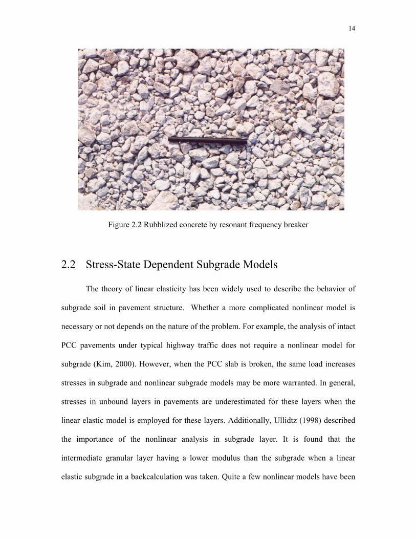
Figure 2.1 shows a resonant frequency breaker operating on US 29, and Figure
2.2 shows rubblized concrete. The resonant frequency breaker gives a low amplitude (0.5
in or 13 mm) and a high frequency resonant energy delivered to the PCC slab, and causes
a high tension at the surface (Niederquell et al., 2000).
Figure 2.1 Resonant frequency breaker
14
Figure 2.2 Rubblized concrete by resonant frequency breaker
2.2 Stress-State Dependent Subgrade Models
The theory of linear elasticity has been widely used to describe the behavior of
subgrade soil in pavement structure. Whether a more complicated nonlinear model is
necessary or not depends on the nature of the problem. For example, the analysis of intact
PCC pavements under typical highway traffic does not require a nonlinear model for
subgrade (Kim, 2000). However, when the PCC slab is broken, the same load increases
stresses in subgrade and nonlinear subgrade models may be more warranted. In general,
stresses in unbound layers in pavements are underestimated for these layers when the
linear elastic model is employed for these layers. Additionally, Ullidtz (1998) described
the importance of the nonlinear analysis in subgrade layer. It is found that the
intermediate granular layer having a lower modulus than the subgrade when a linear
elastic subgrade in a backcalculation was taken. Quite a few nonlinear models have been
15
suggested by researchers. In this chapter, these models are briefly described for granular
and fine-grained soils.
2.2.1 Granular Soil
The resilient modulus in granular materials has been known to be stress-state
dependent. Several models have been developed for analyzing the characteristics of
granular materials.
The θ−k model has been the most popular in representing the stress-state
dependency of granular materials. The resilient modulus is expressed as a function of the
bulk stress as follows:
21
kr kM θ= (2.1)
where
Mr = resilient modulus,
θ = bulk stress (= ), and 321 σσσ ++
21,kk = regression constants determined from the repeated triaxial loading test
results.
The contour model proposed by Brown and Pappin (1981) expressed the shear
and volumetric stress-strain relations for granular materials using the stress path to
simulate the actual pavement conditions. Due to the complication of the contour model,
it is difficult to use it as a practical model in characterizing granular materials. Brown and
Pappin also emphasized the importance of effective stress, which is influenced by pore
pressure in partially or totally saturated materials.

16
Uzan (1985) proposed the modified stress-state dependent model expressed in
terms of both deviator and bulk stresses, as shown below. Uzan’s model can account for
the shear stress effect on the resilient modulus.
321
kd
kr kM σθ= (2.2)
where
θ = bulk stress (= ), 321 σσσ ++
dσ = deviator stress (= 31 σσ − ) as defined in Figure 2.3, and
321 ,, kkk = regression constants.
3σ
dσσσ += 31
2σ
32 σσ =
Figure 2.3 Principal stresses on a finite soil element
Elliot and David (1989) provided an improved model to represent the stress
dependent behavior of granular materials above failure state. When the deviator stress
exceeds the stress at failure state, the modulus of granular material tends to decrease with
increasing deviator stress. The developed model is as follows:
A
k
rkM10
21θ= (2.3)
17
where
A = mR3,
21,kk = regression constants, and
R = stress/strength ratio.
The UT-Austin model shown below is obtained from the following procedure:
(1) measure axial strain and stress during a triaxial test,
(2) calculate moduli from the relationship between strain and stress with varying loads,
and
(3) do multi regression to find coefficients (e.g., k1, k2, and k3 ).
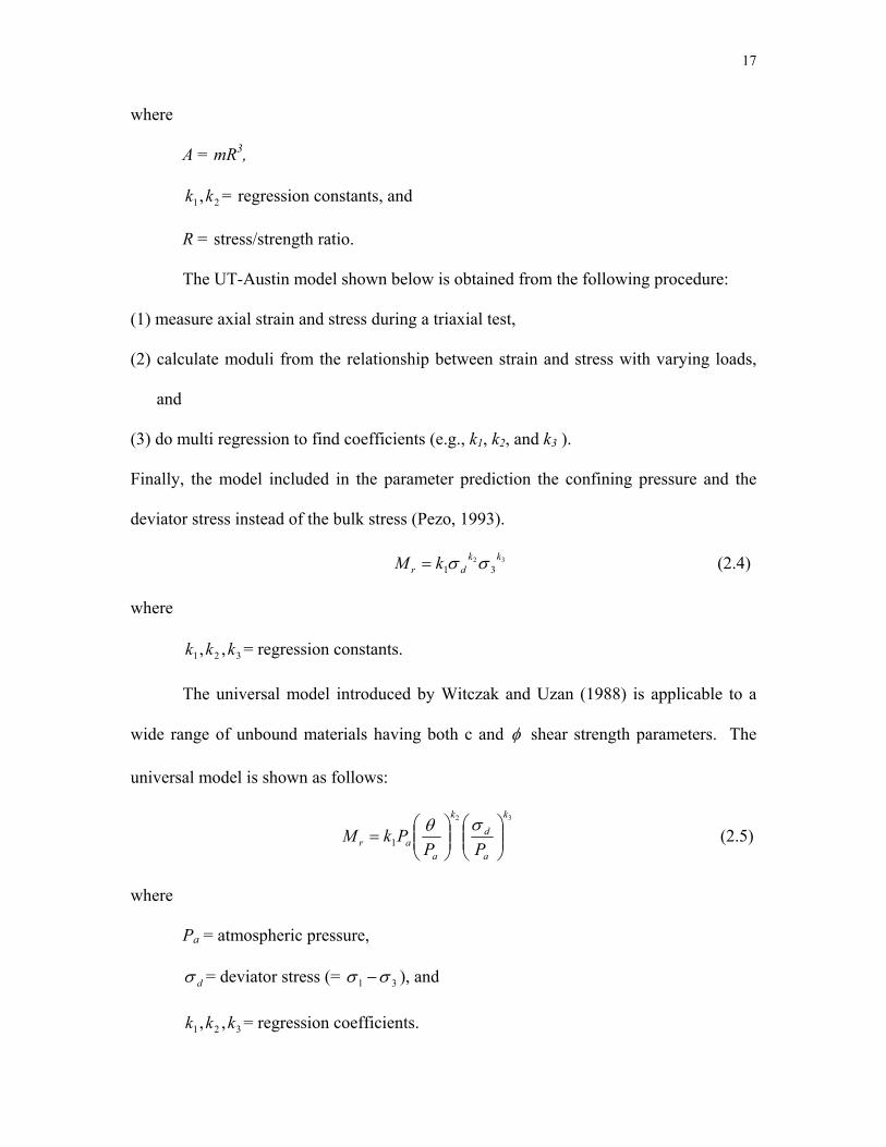
Finally, the model included in the parameter prediction the confining pressure and the
deviator stress instead of the bulk stress (Pezo, 1993).
3231
kkdr kM σσ= (2.4)
where
321 ,, kkk = regression constants.
The universal model introduced by Witczak and Uzan (1988) is applicable to a
wide range of unbound materials having both c and φ shear strength parameters. The
universal model is shown as follows:
32
1
k
a
d
k
aar PP
PkM
=
σθ (2.5)
where
Pa = atmospheric pressure,
dσ = deviator stress (= 31 σσ − ), and
321 ,, kkk = regression coefficients.
18
The comparison of measured and predicted moduli of granular materials showed
that the universal model improved the accuracy of prediction of resilient modulus
significantly (Santha, 1994). In case of fine-grained material, it is recommended to use
this model when test data has a series of confining pressure.
Tutumluer and Thompson (1997) proposed a cross-anisotropic model to predict
the vertical, horizontal, and shear moduli of granular base materials. Unlike the isotropic
elastic model, the nonlinear anisotropic model was able to show the variations of vertical
and horizontal moduli of base materials. It is noted that the horizontal modulus is lower
than the vertical modulus and the tensile stresses at the bottom of base can be reduced
drastically compared to the results from isotropic elastic programs. The summary of
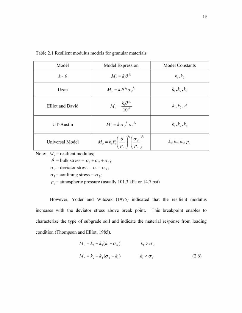
nonlinear models for granular soils is given in Table 2.1.
2.2.2 Fine-Grained Soil
The resilient modulus of fine-grained soil is usually dependent on the deviator
stress and moisture content. In general, it decreases with the increase in deviator stress
(stress-softening effect). The moisture content affects the resilient modulus of fine-
grained soil more significantly than that of granular material (Thadkamalla and George,
1992).
The bilinear model based on repeated axial load test shows that the resilient
modulus drastically decreases as the deviator stress increases up to breakpoint, and then
slightly decreases.
19
Table 2.1 Resilient modulus models for granular materials
Model Model Expression Model Constants
k - θ 21
kr kM θ= 21,kk
Uzan 321
kd
kr kM σθ= 321 ,, kkk
Elliot and David A
k
rkM10
21θ= Akk ,, 21
UT-Austin 3231
kkdr kM σσ= 321 ,, kkk
Universal Model 32
1
k
a
d
k
aar pp
PkM
=
σθ apkkk ,,, 321
Note: = resilient modulus; rM θ = bulk stress = 321 σσσ ++ ; dσ = deviator stress = 31 σσ − ; 3σ = confining stress = 2σ ; = atmospheric pressure (usually 101.3 kPa or 14.7 psi) ap
However, Yoder and Witczak (1975) indicated that the resilient modulus
increases with the deviator stress above break point. This breakpoint enables to
characterize the type of subgrade soil and indicate the material response from loading
condition (Thompson and Elliot, 1985).
)( 132 dr kkkM σ−+= k dσ>1
)( 142 kkkM dr −+= σ k dσ<1 (2.6)
20
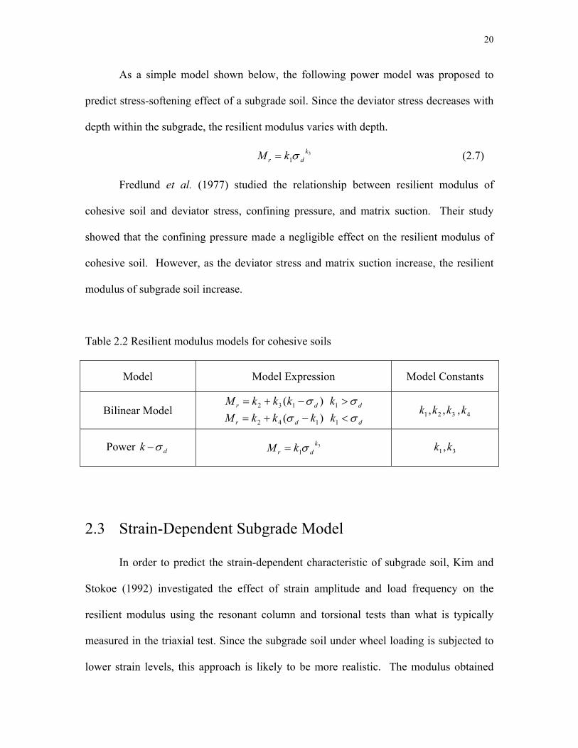
As a simple model shown below, the following power model was proposed to
predict stress-softening effect of a subgrade soil. Since the deviator stress decreases with
depth within the subgrade, the resilient modulus varies with depth.
31
kdr kM σ= (2.7)
Fredlund et al. (1977) studied the relationship between resilient modulus of
cohesive soil and deviator stress, confining pressure, and matrix suction. Their study
showed that the confining pressure made a negligible effect on the resilient modulus of
cohesive soil. However, as the deviator stress and matrix suction increase, the resilient
modulus of subgrade soil increase.
Table 2.2 Resilient modulus models for cohesive soils
Model Model Expression Model Constants
Bilinear Model )( 132 dr kkkM σ−+= dk σ>1 )( 142 kkkM dr −+= σ dk σ<1 4321 ,,, kkkk
Power k dσ− 31
kdr kM σ= 31,kk
2.3 Strain-Dependent Subgrade Model
In order to predict the strain-dependent characteristic of subgrade soil, Kim and
Stokoe (1992) investigated the effect of strain amplitude and load frequency on the
resilient modulus using the resonant column and torsional tests than what is typically
measured in the triaxial test. Since the subgrade soil under wheel loading is subjected to
lower strain levels, this approach is likely to be more realistic. The modulus obtained
21
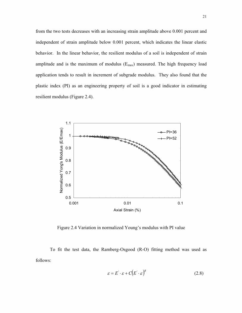
from the two tests decreases with an increasing strain amplitude above 0.001 percent and
independent of strain amplitude below 0.001 percent, which indicates the linear elastic
behavior. In the linear behavior, the resilient modulus of a soil is independent of strain
amplitude and is the maximum of modulus (Emax) measured. The high frequency load
application tends to result in increment of subgrade modulus. They also found that the
plastic index (PI) as an engineering property of soil is a good indicator in estimating
resilient modulus (Figure 2.4).
0.5
0.6
0.7
0.8
0.9
1
1.1
0.001 0.01 0.1
Axial Strain (%)
Nor
mal
ized
Yon
g's
Mod
ulus
(E/E
max
)
PI=36PI=52
Figure 2.4 Variation in normalized Young’s modulus with PI value
To fit the test data, the Ramberg-Osgood (R-O) fitting method was used as
follows:
( )RECE εεε ⋅+⋅= '' (2.8)
22
where
max' / EEE = = normalized Young’s modulus and
C and R = R-O parameters.
Equation (2.8) can be rearranged:
RECE )()1( '' εε ⋅⋅=−⋅ (2.9)
By taking the logarithm of both sides, Equation (2.9) gives:
)log(log)]1(log[ '' εε ⋅⋅+=−⋅ ERCE (2.10)
Based on a least-squares method, the R-O parameter R is directly determined
from the slope, and the parameter C is obtained from the intercept. This strain approach
has an advantage that a single regressed model takes care of cohesive materials
comparing to the stress-based models. However, the strain-based model is not accurate
for granular soils because it cannot account for bulk stresses.
Borden et al. (1994) studied the soil response induced by vibration, which is
similar to a pavement system under moving traffic loads using laboratory resonant
column and torsional shear tests. They investigated the effects of soil types, confining
pressure, shear strain amplitude, and number of cycles applied using resonant column and
torsional shear tests. It is found that the shear modulus of the residual soils decreased and
the damping ratio increased with an increasing shear strain amplitude. In addition, no
significant effect of number of cycles was found on the shear modulus and damping ratio
of residual soils.
23
CHAPTER THREE PCC PAVEMENT ANALYSIS
The multi-layered linear elastic theory is not appropriate for the study of the
behavior of subgrade under intact and rubblized PCC pavements because of its inability
to account for stress-state dependence of soils. Rather, the finite element method (FEM)
is the most accurate means for calculating pavement response. Finite element models are
able to simulate the results of proven theories such as the multi-layered elastic theory
and, further, allow the possibility of adding more complicated material models, such as
stress-state dependent subgrade model, to pavement analysis.
Several finite element programs have been developed for pavement structural
analyses, such as ILLI-PAVE and MICH-PAVE for flexible pavements and ILLI-SLAB
for rigid pavements. The ILLI-PAVE computer program considers an axisymmetric
structure for finite mesh generation and the stress-state dependent modulus for granular
materials and cohesive soils. The principal stresses in granular and cohesive soils are
changed at the end of iterations into a Morhr-Coulomb failure envelope if the deviator
stress exceeds the failure envelope.
In this study, a commercially available finite element program, ABAQUS, was
used to compute pavement responses based on dynamic analysis. Additionally,
NCPAVE, recently developed by researchers at North Carolina State University, was
used for static analysis with FWD multi-level loads. Issues related to the finite element
modeling of PCC pavements under multi-level FWD loads are discussed in the remainder
of this chapter.

24
3.1 FEM Program
ABAQUS has been proven suitable for pavement analysis by many researchers.
Kuo et al. (1995) conducted a comprehensive study of various FEM pavement analysis
programs and showed that the ABAQUS program yields results comparable to those of
other programs. Zaghoul and White (1993) successfully employed ABAQUS for 3-D
dynamic analysis of intact flexible pavements. Three-dimensional rigid pavement
analyses using ABAQUS were also performed by Kuo et al. (1995), Mallela and George
(1994), and Zaghloul et al. (1993). In addition, Uddin et al. (1995) investigated the
behavior of a jointed concrete pavement under a standard FWD load with discontinuities,
such as joint deterioration and transverse cracking, using ABAQUS with 3-D dynamic
analysis.
ABAQUS provides many element and material models that are useful for
pavement analysis. For example, the infinite element model may be used to model the
infinite horizontal and vertical boundaries of a pavement profile with static, harmonic,
and transient dynamic loading and thermal gradient conditions. In the case of a material
model, ABAQUS is available with linear elastic, nonlinear elastic, viscoelastic, plastic,
and modified elastic.
In this study, the finite element method using ABAQUS is applied to analyze
pavement systems with dynamic loads, an axisymmetric structure, and a nonlinear
subgrade model.
NCPAVE, a static finite element program, was developed to generate a database
of deflections dependent on pavement structures and material properties. The finite
element method using NCPAVE is the same as that of ABAQUS with the exception of

25
static analysis. In addition, NCPAVE serves as a stand-alone forward model to give
surface deflections based on backcalculated subgrade characteristics and pavement
structures.
3.2 Nonlinearity Using FWD Multi-Level Loads
To predict the stress-state dependence of subgrade soils under PCC slabs, a multi-
level load FWD test may be used. The underlying assumption is that the stress state of
subgrade after rubblization can be reproduced by applying a higher FWD load on a PCC
slab prior to rubblization. The multi-level loads and backcalculated subgrade moduli
allow the establishment of a stress-state dependent subgrade modulus relationship that
may be used to predict the subgrade response after rubblization.
The significance of nonlinearity in the analysis of multi-load FWD deflections
should be considered to determine whether multi-level loads cause enough nonlinearity in
the subgrade. According to AASHTO (1993), the ratio of loads will be equal to the
deflection ratio if the material is linear.
That is,
r
rd
dP
P2
1
2
1 = or rr d
Pd
P2
2
1
1 = (3.1)
where
1P = load 1 ,
2P = load 2,
rd1 = measured deflection at a radial distance under FWD load 1, and
rd2 = measured deflection at a radial distance under FWD load 2.
26
The nonlinearity in the analysis of multi-load FWD deflection measured from
intact PCC slab has been investigated using the deflection data measured from US 29.
This pavement has a 14 inch thick PCC slab over cohesive soil. (Structural details of this
pavement, along with the FWD test procedure, is presented later in Chaper 5.) To
determine the amount of nonlinearity in the deflections, the center and seventh
deflections were normalized with respect to the load level and plotted against the load
level. In such a plot, the deviation from a horizontal line indicates the amount of
nonlinearity in the system.
The data from five stations of US 29 have been analyzed and are plotted in Figure
3.1. It appears that nonlinear behavior is exhibited in all the stations in varying degrees.
The degree of nonlinearity was calculated by dividing the difference in the normalized
deflections under 9 and 15 kip loads by the deflection under the 9 kip load. The highest
degree of nonlinearity was found to be around 14 % (Figure 3.2).
Based on this analysis, the multi-level loads (9, 12, and 15 kip FWD loads) cause
sufficiently high stresses in subgrade under intact PCC slab. It is assumed that the
deflections measured from FWD tests are appropriate to estimate the nonlinear
characteristics of subgrade.
3.3 Forward Model
The development of a procedure for determining stress-state dependent properties
of subgrade from multi-load deflections requires a forward model that can predict stresses
in the subgrade under varying upper layer conditions. Based on the literature review in
27
Chapter 2 on pavement response models and nonlinear material models of subgrade, the
ABAQUS finite element program was selected as the pavement response model, using
Uzan’s stress-state dependent model for subgrade. Dynamic analysis was performed
using ABAQUS with axisymmetric finite element representation of a pavement structure.
Details of the finite element analysis are described below. Figure 3.3 shows the input
loading history to simulate the FWD load. A haver-sine wave form with 0.03 second
duration was used.
A pavement system is modeled with an infinite boundary in the lateral direction
and with semi-infinite depth for the subgrade layer. Since the area near the load is
subjected to high stresses and strains compared to the boundary medium, the surface
region of the model uses smaller element than those of the subgrade. This element
structure is shown in Figure 3.4.
Due to the complexities involved in the analysis of deflections measured near
joints or edges in PCC pavements, it is assumed that FWD tests were performed in the
middle of a slab. This assumption makes axisymmetric representation of the load and
pavement more realistic.
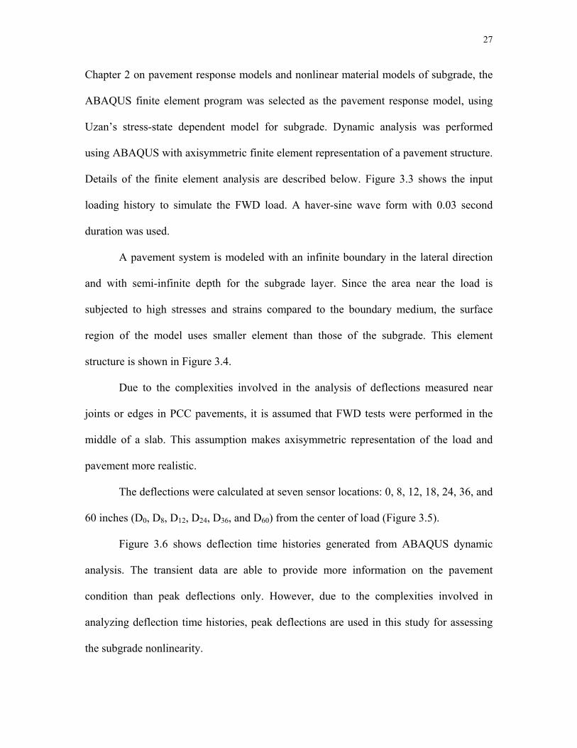
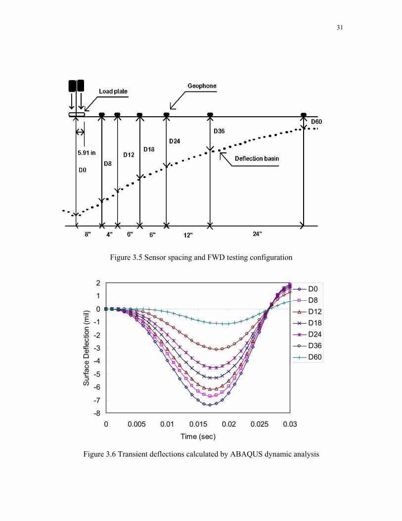
The deflections were calculated at seven sensor locations: 0, 8, 12, 18, 24, 36, and
60 inches (D0, D8, D12, D24, D36, and D60) from the center of load (Figure 3.5).
Figure 3.6 shows deflection time histories generated from ABAQUS dynamic
analysis. The transient data are able to provide more information on the pavement
condition than peak deflections only. However, due to the complexities involved in
analyzing deflection time histories, peak deflections are used in this study for assessing
the subgrade nonlinearity.

28
0.0003
0.00035
0.0004
0.00045
0.0005
0.00055
0.0006
0.00065
0.0007
9 12 15
Load Level (kip)
Norm
alize
d D
efle
ctio
n (m
il/lb
)
Station 198Station 215Station 216Station 237Station 308
(a)
0.00005
0.0001
0.00015
0.0002
0.00025
0.0003
0.00035
9 12 15
Load Level (kip)
Norm
alize
d D
efle
ctio
n (m
il/lb
)
Station 198Station 215Station 216Station 237Station 308
(b)
Figure 3.1 Normalized deflection vs. load level: (a) center deflection and (b) seventh deflection

29
0.0
2.0
4.0
6.0
8.0
10.0
12.0
14.0
16.0
190 200 210 220 230 240 250 260 270 280 290 300 310 320
Station Number
Deg
ree
of N
onlin
erity
Degree of Nonlinearity
Figure 3.2 Degree of nonlinearity from US 29 FWD tests [(D0 under 15kip – D0 under 9kip)/D0 under 9kip]

30
00.10.20.30.40.50.60.70.80.9
1
0 0.005 0.01 0.015 0.02 0.025 0.03
Time (sec)
Nor
mal
ized
App
lied
Load
Am
plitu
de
Figure 3.3 Normalized load used for dynamic analysis
Figure 3.4 Infinite element model of a pavement system
31
Figure 3.5 Sensor spacing and FWD testing configuration
1
-8
-7
-6
-5
-4
-3
-2
-1
0
2
0 0.005 0.01 0.015 0.02 0.025 0.03Time (sec)
Surfa
ce D
efle
ctio
n (m
il)
D0D8D12D18D24D36D60
Figure 3.6 Transient deflections calculated by ABAQUS dynamic analysis
32
3.4 Dynamic vs. Static Analysis
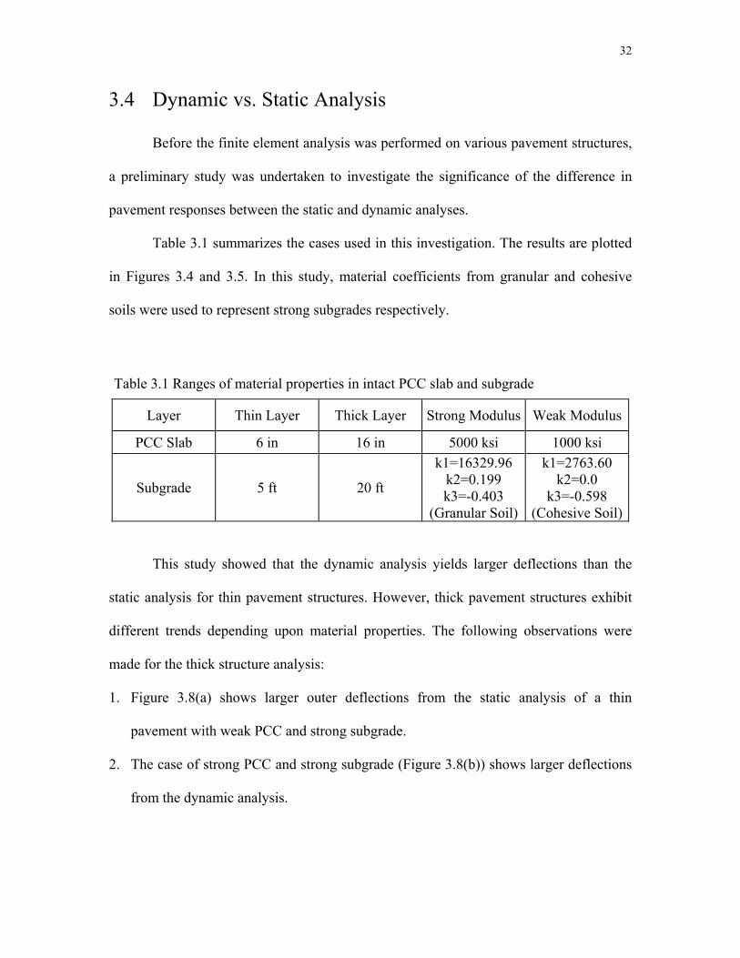
Before the finite element analysis was performed on various pavement structures,
a preliminary study was undertaken to investigate the significance of the difference in
pavement responses between the static and dynamic analyses.
Table 3.1 summarizes the cases used in this investigation. The results are plotted
in Figures 3.4 and 3.5. In this study, material coefficients from granular and cohesive
soils were used to represent strong subgrades respectively.
Table 3.1 Ranges of material properties in intact PCC slab and subgrade
Layer Thin Layer Thick Layer Strong Modulus Weak Modulus
PCC Slab 6 in 16 in 5000 ksi 1000 ksi
Subgrade 5 ft 20 ft
k1=16329.96 k2=0.199 k3=-0.403
(Granular Soil)
k1=2763.60 k2=0.0
k3=-0.598 (Cohesive Soil)
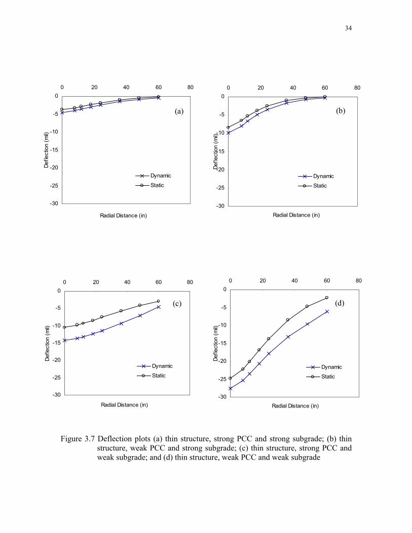
This study showed that the dynamic analysis yields larger deflections than the
static analysis for thin pavement structures. However, thick pavement structures exhibit
different trends depending upon material properties. The following observations were
made for the thick structure analysis:
1. Figure 3.8(a) shows larger outer deflections from the static analysis of a thin
pavement with weak PCC and strong subgrade.
2. The case of strong PCC and strong subgrade (Figure 3.8(b)) shows larger deflections
from the dynamic analysis.

33
3. Figures 3.8(c) and (d) (e.g., strong PCC and weak subgrade and weak PCC and weak
subgrade) demonstrate that the static analysis generates larger deflections than the
dynamic analysis.
34
-30
-25
-20
-15
-10
-5
00 20 40 60 80
Radial Distance (in)
Defle
ctio
n (m
il)
Dynamic
Static
(a)
-30
-25
-20
-15
-10
-5
00 20 40 60 80
Radial Distance (in)De
flect
ion
(mil)
Dynamic
Static
(b)
-30
-25
-20
-15
-10
-5
00 20 40 60 80
Radial Distance (in)
Defle
ctio
n (m
il)
Dynamic
Static
(c)
-30
-25
-20
-15
-10
-5
00 20 40 60 8
Radial Distance (in)
Defle
ctio
n (m
il)
Dynamic
Static
(d)
0
Figure 3.7 Deflection plots (a) thin structure, strong PCC and strong subgrade; (b) thin structure, weak PCC and strong subgrade; (c) thin structure, strong PCC and weak subgrade; and (d) thin structure, weak PCC and weak subgrade
35
-10
-8
-6
-4
-2
00 20 40 60 80
Radial Distance (in)
Defle
ctio
n (m
il)
Dynamic
Static
(a)
-10
-8
-6
-4
-2
00 20 40 60 80
Radial Distance (in)
Defle
ctio
n (m
il)
Dynamic
Static
(b)
-10
-8
-6
-4
-2
00 20 40 60 80
Radial Distance (in)
Defle
ctio
n (m
il)
Dynamic
Static
(c)
-10
-8
-6
-4
-2
00 20 40 60 80
Radial Distance (in)
Defle
ctio
n (m
il)
Dynamic
Static
(d)
Figure 3.8 Deflection plots (a) thick structure, strong PCC and strong subgrade; (b) thick structure, weak PCC and strong subgrade; (c) thick structure, strong PCC and weak subgrade; and (d) thick structure, weak PCC and weak subgrade
36
CHAPTER FOUR SUBGRADE CONDITION PREDICTION
ALGORITHMS USING ANN
One of the backcalculation techniques used extensively in this research is that of
artificial neural networks (ANNs). The strength of this approach (i.e., fast inversion once
it is trained) is especially attractive because it counteracts the significant amount of time
taken by the iterative method that is based on error minimization and that is integral to
the complex forward model chosen in this research. This chapter describes the research
effort that uses ANNs in different ways to predict the nonlinear characteristics of
subgrade from deflections measured on PCC slabs.
In summary, ANNs were trained using the synthetic database to predict Uzan’s
model coefficients ( , , and k ) in Equation (2.2) and the strain-based model
coefficients (C and R) in Equation (2.8) from multi-level load FWD deflections. ANNs
were used in different ways to develop a method that would yield satisfactory
performance for a set of test cases in the synthetic database. For the stress-based
approach, an attempt was made to predict the nonlinear coefficients without knowing the
soil type (i.e., granular versus cohesive) a priori. Poor performance from this approach
suggested the need to investigate the development of an ANN-based model for cohesive
soils only. Only k
1k 2k 3
1 and k3 were predicted in this case, and improved performance resulted
from this approach. The following sections describe all the efforts made in these different
approaches using ANN.

37
4.1 Stress-Based ANN Model for General Soils
Estimation of nonlinear characteristics of subgrade using ANN requires a large
database comprised of various pavement structures and layer properties. ABAQUS was
run in the axisymmetric, dynamic mode with Uzan’s model for subgrade to simulate the
intact PCC pavement responses under multi-load FWD tests. For the static analysis,
NCPAVE was run using the same structures and layer properties as in the dynamic
analysis.
The input variables needed in the forward modeling include:
a) load level (9, 12, and 15 kips)
b) thickness of PCC slab (Hpcc)
c) modulus of PCC slab (Epcc)
d) thickness of subgrade (Hsg)
e) Uzan’s model coefficients ( , , and ) 1k 2k 3k
The ranges of these input variables for forward modeling are shown in Table 4.1.
Table 4.1 The ranges of the input variables for forward modeling
Thickness Modulus (ksi) Layer
Min. Max. Increment Min. Max. Increment
Intact PCC 6 in 16 in 1 in 500 5,000 100
Subgrade 2 ft 20 ft 1 ft *45 cases for granular soils and 42 cases for cohesive soils
Note : *Obtained from Lanka Santha’s (1994) laboratory study of various soil’s stress-state dependencies represented by Uzan’s model
In Table 4.1, the maximum and minimum layer thicknesses were determined by
investigating all the PCC pavement cases registered in DataPave. The PCC slab thickness
38
and the subgrade thickness together determine the depth to a stiff layer. The PCC slab
modulus range was determined from the literature. For the subgrade modulus, a
comprehensive summary of Uzan’s model coefficients on various granular and cohesive
soils is available in Santha (1994). These coefficients were used to represent varying soil
types in pavement systems.
Random combinations of input properties were generated using the Latin
hypercube random sampling technique to provide even distribution of the input properties
within the ranges and the increments defined by the user. At first, a total of 2,000 cases
was created for each load level. Later, 200 cases containing low moduli (500 to 900 ksi)
for PCC were included to consider the case of FWD tests on distressed PCC pavements.
A total of 6,600 cases (2,200 cases for each of the three load levels) was modeled for the
database. Out of 6,600 cases, 6,000 randomly selected cases (2,000 cases per load level)
were used to train the ANN to establish the relationship between Uzan’s model
coefficients and surface deflections. This relationship is represented by a network with
adjusting weights and biases that yield the minimum error for prediction.
The remaining 600 cases were used for testing the trained ANN. A typical change
of root-mean-square-error (RMSE) as a function of epochs (i.e., trained iterations) is
shown. The optimum weights and biases in the ANN were selected when the testing
RMSE was the lowest. The optimum ANN structure was determined by systematically
changing the number of hidden layers and units and selecting the structure that yielded
the lowest training and testing RMSEs.
39
If the network is trained too much, the network will learn the noise or memorize
the training patterns and will not generalize well with new patterns (Kim, 1997). To
prevent overtraining and in order to select an optimum structure that yields the lowest
RMSE from testing, an independent testing set (100 randomly selected cases) was used as
well as the training set. As shown in Figure 4.1, there is an optimum point where the
testing RMSE starts to increase even though the training RMSE decreases. The
network’s weights at this optimum point of the lowest testing RMSE were saved.
0
5
10
15
20
25
30
35
40
0 200 400 600 800 1000 1200Number of Epochs
RM
SE
Testing RMSETraining RMSE
Optimum Point
Figure 4.1 Finding optimum point using testing set
40
4.1.1 Direct Backcalculation
In this approach, 21 deflections generated by 3 load levels were used as inputs to
directly predict , , and . Many different hidden layer structures were tried with and
without the PCC thickness as an additional input. Table 4.2 summarizes the best two
structures for each of the two cases. In general, RMSEs were not satisfactory. The
prediction of was much more difficult, and the inclusion of Hpcc as an additional
input improved the prediction accuracy.
1k
2
2k 3k
k
In order to find whether this poor prediction was due to the nature of dynamic
analysis, NCPAVE was run in the static mode to develop a database that may be used to
train ANNs. All other analysis features in NCPAVE were kept the same as those in
ABAQUS. Using the ANNs trained by the static database, Uzan’s coefficients were
backcalculated and the prediction errors were compared with those from the dynamic
backcalculation. It can be concluded from Table 4.3 that the static analysis does not
improve the prediction accuracy compared to the dynamic analysis. This poor prediction
from the direct backcalculation approach thereby required investigation into another
approach which is explained in the next section.
4.1.2 Regression Approach Using ANN Backcalculated Stresses and Moduli
The regression approach is based on the observation that the prediction of
pavement responses (e.g., stresses and strains) and the subgrade modulus from surface
deflections is much more promising than the prediction of subgrade nonlinear properties.
Once stresses and subgrade moduli are predicted, a regression analysis of them can yield
41
Uzan's model coefficients. The static nonlinear finite element analysis was performed on
various pavement structures to compute pavement deflections and bulk and deviator in
subgrade under the center of the load. Uzan's model was used for subgrade; subgrade
moduli at the end of the iterations of the finite element analysis were stored in the
database.
Table 4.2 Prediction RMSEs of k , k , and using dynamic database 1 2 3k
Input Hidden layer Structure Output
Training Average
RMSE*(%)
Testing Average
RMSE (%) 1k 43.60 45.55
2k 93.30 185.26 D0 to D60 under Multi-loads 21-25-22-1
3k 3.41 12.22
1k 22.35 30.0
2k 70.50 190.20 D0 to D60 under Multi-loads 21-26-23-1
3k 4.98 11.84
1k 10.49 35.76
2k 98.64 194.17 D0 to D60 under
Multi-loads Hpcc**
22-25-22-1
3k 5.58 11.23
1k 18.70 27.11
2k 69.35 220.0 D0 to D60 under
Multi-loads Hpcc
22-26-23-1
3k 5.98 12.84 *RMSE : Root Mean Square Error ** Hpcc : PCC slab thickness
ANNs were trained using this database to predict subgrade moduli and bulk and
deviator stresses at the top of the subgrade from surface deflections caused by 9, 12, 15
kip load levels. The accuracy of the prediction is tabulated in Tables 4.4 to 4.6. In all the
cases, the testing RMSEs were below 10%, thus indicating satisfactory prediction.
42
Table 4.3 Prediction RMSEs of k , k , and using static database 1 2 3k
Input Hidden Layer Output Training Average
RMSE (%)
Testing Average
RMSE (%)
1k 24.91 26.69
2k 166.17 251.62 D0 to D60 under Multi-loads 21-25-22-1
3k 21.86 32.23
1k 21.07 26.73
2k 192.40 265.14 D0 to D60 under Multi-loads 21-26-23-1
3k 25.17 29.34
Table 4.4 Prediction accuracy of the indirect backcalculation using deflections under 9 kip FWD load
Input Hidden layer Structure Output
Training Average
RMSE (%)
Testing Average
RMSE (%) 7-14-11-1 1.28 1.74 D0 to D60 7-15-12-1
Center* Bulk Stress 1.48 1.81
7-14-11-1 4.35 4.66 D0 to D60 7-15-12-1 Center Deviator
Stress 4.12 4.68 7-14-11-1 8.73 8.35 7-15-12-1 7.86 8.86 7-16-13-1 8.58 8.47
D0 to D60
7-17-14-1
Center Modulus
8.98 8.97 *Center : The point at the top of the subgrade below the load plate of FWD

43
Table 4.5 Prediction accuracy of the indirect backcalculation using deflections under 12 kip FWD load
Input Hidden layer Structure Output
Training Average
RMSE (%)
Testing Average
RMSE (%) 7-14-11-1 1.63 2.21 D0 to D60 7-15-12-1
Center Bulk Stress 1.88 2.53
7-14-11-1 4.70 4.78 D0 to D60 7-15-12-1 Center Deviator
Stress 4.86 5.49 7-14-11-1 8.45 9.13 7-15-12-1 8.65 9.07 7-16-13-1 7.83 9.52
D0 to D60
7-17-14-1
Center Modulus
8.74 8.84
Table 4.6 Prediction accuracy of the indirect backcalculation using deflections under 15 kip FWD load
Input Hidden layer Structure Output
Training Average
RMSE (%)
Testing Average
RMSE (%) 7-14-11-1 2.23 2.45 D0 to D60 7-15-12-1
Center Bulk Stress 1.72 2.59
7-14-11-1 5.77 6.41 D0 to D60 7-15-12-1 Center Deviator
Stress 4.21 5.19 7-14-11-1 8.49 8.70 7-15-12-1 8.94 9.23 7-16-13-1 8.35 9.80
D0 to D60
7-17-14-1
Center Modulus
6.99 8.50
These ANNs were used to predict the subgrade modulus and bulk and deviator
stresses from synthetic deflections. These predicted values were regressed to determine
, , and . They were then compared with the known values used to generate the
synthetic deflections. The RMSEs were over 100% for estimating all the coefficients. The
comparison was not any better than the accuracy shown in Table 4.2 from the direct
backcalculation. The backcalculation procedure using the stresses under the center of the
1k 2k 3k
44
FWD load and modulus may be sufficient to capture the nonlinearity of subgrade using
the regression approach.
Based on the prediction results from the two approaches, reliable backcalculation
of Uzan’s model coefficients is not feasible without having more information presented
to the ANN as inputs. A subgrade soil type that can be obtained by construction record or
by sampling from outside shoulder areas can provide the soil type (i.e., granular versus
cohesive) and may be used as an additional input. The following section describes this
procedure.
4.2 Stress-Based ANN Model for Cohesive Soils
Since most of the problematic soils in pavements are categorized as cohesive
soils, the research effort focused on nonlinear characterization of cohesive soils. This
additional input allowed the value in Uzan's model to be set to equal zero; thus, the
effect of bulk stress in cohesive soils is considered minimal.
2k
Synthetic deflections were obtained using the ABAQUS dynamic analysis with
various material properties and thicknesses. Since the laboratory resilient modulus data
from I-85 soils were available at this time, these coefficients were also included in the
input database. The larger thicknesses and material properties selected for the forward
modeling are summarized in Table 4.7.
One thousand cases were generated randomly with these ranges. Surface
deflections and deviator stresses were calculated on the pavement surface and on the
subgrade at radial distances of 0, 8, 12, 18, 24, 36, and 60 inches (Figure 4.2).

45
Table 4.7 Material properties and thicknesses used in ABAQUS FEM
PCC Layer Subgrade Modulus
(ksi) or
Model Constants
500 ~ 5,000 (ksi)
42 sets from Santha(1994)
3 sets from lab tests*
Thickness 2 ~ 20 ft 6 ~ 16 in * Resilient modulus tests using cohesive soils from I-85
24 in. 12 in. 6 in. 6 in. 4 in. 8 in.
Subgrade
PCC Slab
Geophone Load Plate
Calculated Stress and Modulus Points
Calculated Deflection Points
Figure 4.2 Locations of calculated deflections, deviator stresses, and moduli
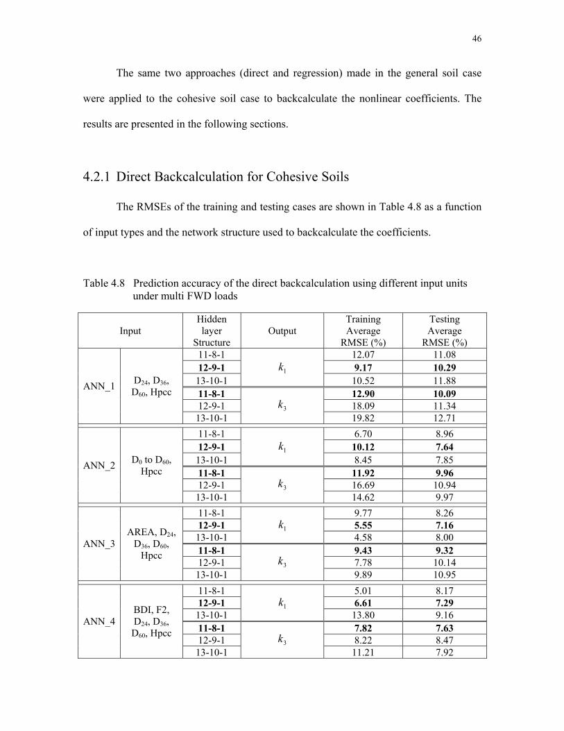
46
The same two approaches (direct and regression) made in the general soil case
were applied to the cohesive soil case to backcalculate the nonlinear coefficients. The
results are presented in the following sections.
4.2.1 Direct Backcalculation for Cohesive Soils
The RMSEs of the training and testing cases are shown in Table 4.8 as a function
of input types and the network structure used to backcalculate the coefficients.
Table 4.8 Prediction accuracy of the direct backcalculation using different input units under multi FWD loads
Input Hidden layer
Structure Output
Training Average
RMSE (%)
Testing Average
RMSE (%) 11-8-1 12.07 11.08 12-9-1 9.17 10.29
13-10-1 1k
10.52 11.88 11-8-1 12.90 10.09 12-9-1 18.09 11.34
ANN_1 D24, D36, D60, Hpcc
13-10-1 3k
19.82 12.71
11-8-1 6.70 8.96 12-9-1 10.12 7.64
13-10-1 1k
8.45 7.85 11-8-1 11.92 9.96 12-9-1 16.69 10.94
ANN_2 D0 to D60, Hpcc
13-10-1 3k
14.62 9.97
11-8-1 9.77 8.26 12-9-1 5.55 7.16
13-10-1 1k
4.58 8.00 11-8-1 9.43 9.32 12-9-1 7.78 10.14
ANN_3 AREA, D24,
D36, D60, Hpcc
13-10-1 3k
9.89 10.95
11-8-1 5.01 8.17 12-9-1 6.61 7.29
13-10-1 1k
13.80 9.16 11-8-1 7.82 7.63 12-9-1 8.22 8.47
ANN_4 BDI, F2, D24, D36, D60, Hpcc
13-10-1 3k
11.21 7.92
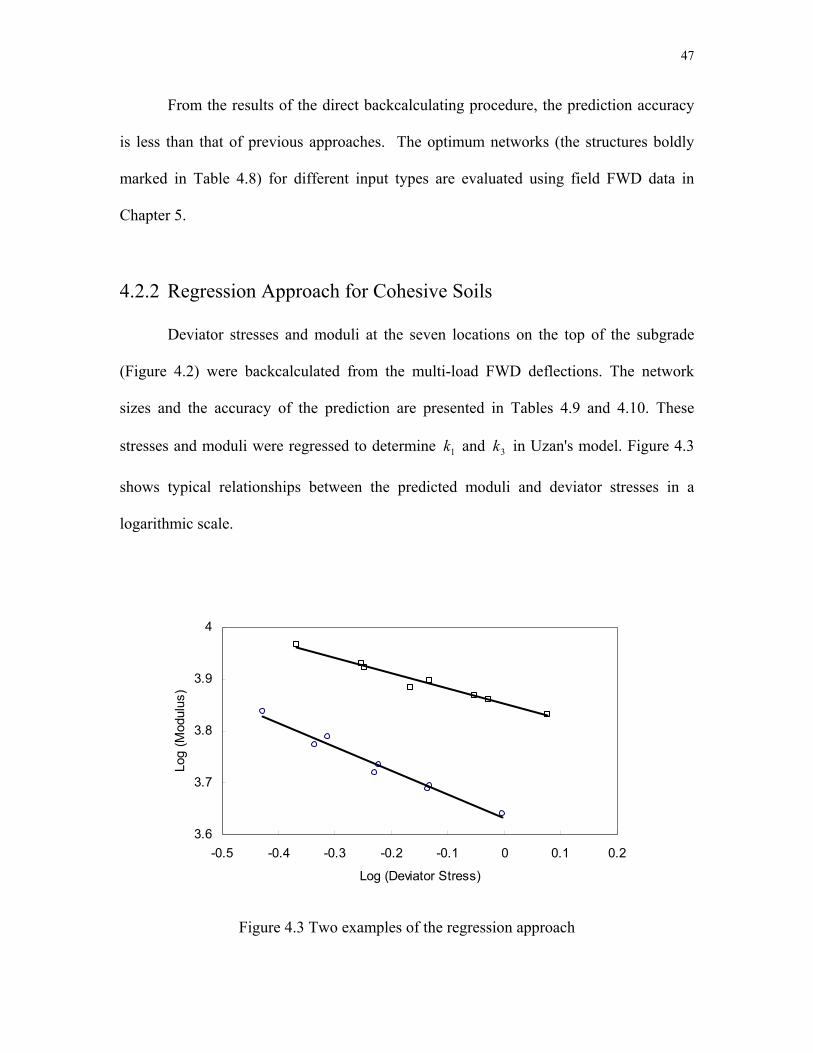
47
From the results of the direct backcalculating procedure, the prediction accuracy
is less than that of previous approaches. The optimum networks (the structures boldly
marked in Table 4.8) for different input types are evaluated using field FWD data in
Chapter 5.
4.2.2 Regression Approach for Cohesive Soils
Deviator stresses and moduli at the seven locations on the top of the subgrade
(Figure 4.2) were backcalculated from the multi-load FWD deflections. The network
sizes and the accuracy of the prediction are presented in Tables 4.9 and 4.10. These
stresses and moduli were regressed to determine and in Uzan's model. Figure 4.3
shows typical relationships between the predicted moduli and deviator stresses in a
logarithmic scale.
1k 3k
3.6
3.7
3.8
3.9
4
-0.5 -0.4 -0.3 -0.2 -0.1 0 0.1 0.2
Log (Deviator Stress)
Log
(Mod
ulus
)
Figure 4.3 Two examples of the regression approach
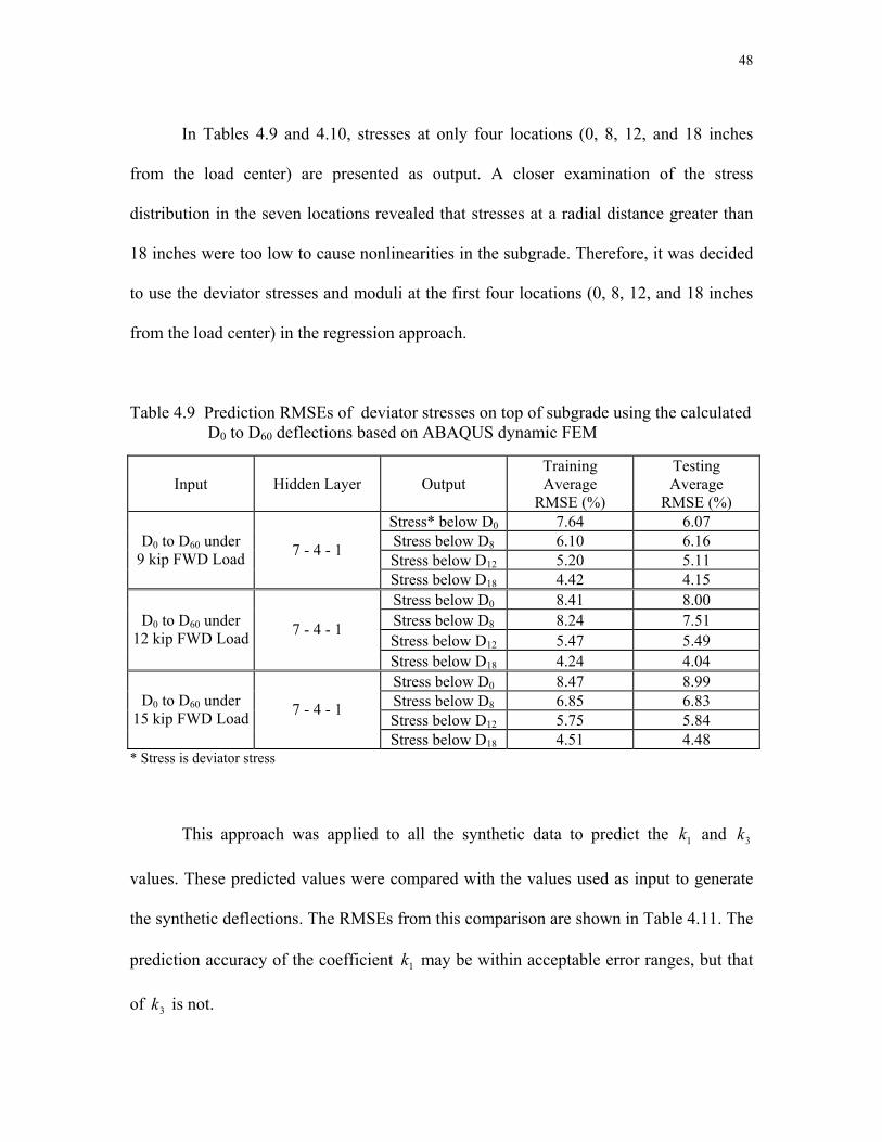
48
In Tables 4.9 and 4.10, stresses at only four locations (0, 8, 12, and 18 inches
from the load center) are presented as output. A closer examination of the stress
distribution in the seven locations revealed that stresses at a radial distance greater than
18 inches were too low to cause nonlinearities in the subgrade. Therefore, it was decided
to use the deviator stresses and moduli at the first four locations (0, 8, 12, and 18 inches
from the load center) in the regression approach.
Table 4.9 Prediction RMSEs of deviator stresses on top of subgrade using the calculated D0 to D60 deflections based on ABAQUS dynamic FEM
Input Hidden Layer Output Training Average
RMSE (%)
Testing Average
RMSE (%) Stress* below D0 7.64 6.07 Stress below D8 6.10 6.16 Stress below D12 5.20 5.11
D0 to D60 under 9 kip FWD Load 7 - 4 - 1
Stress below D18 4.42 4.15 Stress below D0 8.41 8.00 Stress below D8 8.24 7.51 Stress below D12 5.47 5.49
D0 to D60 under 12 kip FWD Load 7 - 4 - 1
Stress below D18 4.24 4.04 Stress below D0 8.47 8.99 Stress below D8 6.85 6.83 Stress below D12 5.75 5.84
D0 to D60 under 15 kip FWD Load 7 - 4 - 1
Stress below D18 4.51 4.48 * Stress is deviator stress
This approach was applied to all the synthetic data to predict the and
values. These predicted values were compared with the values used as input to generate
the synthetic deflections. The RMSEs from this comparison are shown in Table 4.11. The
prediction accuracy of the coefficient k may be within acceptable error ranges, but that
of is not.
1k 3k
1
3k

49
Table 4.10 Prediction RMSEs of moduli on top of subgrade using the calculated D0 to D60 deflections based on ABAQUS dynamic FEM
Input Hidden Layer Output Training Average
RMSE (%)
Testing Average
RMSE (%) Modulus below D0 10.07 7.07 Modulus below D8 9.36 7.48 Modulus below D12 9.14 7.14
D0 to D60 under 9 kip FWD Load 7 - 4 - 1
Modulus below D18 11.89 7.69 Modulus below D0 10.95 8.62 Modulus below D8 11.95 8.29 Modulus below D12 10.48 8.83
D0 to D60 under 12 kip FWD Load 7 - 4 - 1
Modulus below D18 10.22 8.36 Modulus below D0 12.57 10.23 Modulus below D8 11.00 8.14 Modulus below D12 9.59 7.72
D0 to D60 under 15 kip FWD Load 7 - 4 - 1
Modulus below D18 10.46 8.40
Table 4.11 Prediction accuracy of the regression approach
RMSE of (%) 1k RMSE of (%) 3kTraining Case 18.39 60.67 Testing Case 17.12 56.51
Table 4.12 Prediction RMSEs of stresses on top of subgrade using the calculated D0 to D24 deflections based on ABAQUS dynamic FEM
Input Hidden Layer Output Training Average
RMSE (%)
Testing Average
RMSE (%) Stress below D0 11.47 14.57 Stress below D8 8.56 10.60 Stress below D12 7.96 9.01
D0 to D24 under 9 kip FWD Load 10 – 7 - 1
Stress below D18 6.77 7.77 Stress below D0 10.95 12.19 Stress below D8 8.67 9.84 Stress below D12 8.81 9.06
D0 to D24 under 12 kip FWD Load 10 – 7 - 1
Stress below D18 6.59 7.94 Stress below D0 11.89 11.82 Stress below D8 9.89 10.82 Stress below D12 8.02 9.00
D0 to D24 under 15 kip FWD Load 10 – 7 - 1
Stress below D18 6.87 7.44
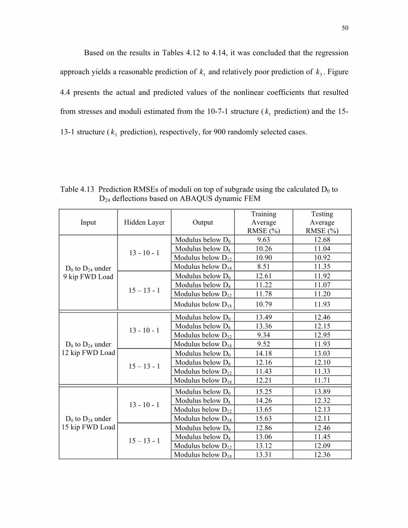
50
Based on the results in Tables 4.12 to 4.14, it was concluded that the regression
approach yields a reasonable prediction of k and relatively poor prediction of . Figure
4.4 presents the actual and predicted values of the nonlinear coefficients that resulted
from stresses and moduli estimated from the 10-7-1 structure ( prediction) and the 15-
13-1 structure ( k prediction), respectively, for 900 randomly selected cases.
1 3k
1k
3
Table 4.13 Prediction RMSEs of moduli on top of subgrade using the calculated D0 to D24 deflections based on ABAQUS dynamic FEM
Input Hidden Layer Output Training Average
RMSE (%)
Testing Average
RMSE (%) Modulus below D0 9.63 12.68 Modulus below D8 10.26 11.04 Modulus below D12 10.90 10.92 13 - 10 - 1
Modulus below D18 8.51 11.35 Modulus below D0 12.61 11.92 Modulus below D8 11.22 11.07 Modulus below D12 11.78 11.20
D0 to D24 under 9 kip FWD Load
15 – 13 - 1
Modulus below D18 10.79 11.93 10.95
Modulus below D0 13.49 12.46 Modulus below D8 13.36 12.15 Modulus below D12 9.34 12.95 13 - 10 - 1
Modulus below D18 9.52 11.93 Modulus below D0 14.18 13.03 Modulus below D8 12.16 12.10 Modulus below D12 11.43 11.33
D0 to D24 under 12 kip FWD Load
15 – 13 - 1
Modulus below D18 12.21 11.71
Modulus below D0 15.25 13.89 Modulus below D8 14.26 12.32 Modulus below D12 13.65 12.13 13 - 10 - 1
Modulus below D18 15.63 12.11 Modulus below D0 12.86 12.46 Modulus below D8 13.06 11.45 Modulus below D12 13.12 12.09
D0 to D24 under 15 kip FWD Load
15 – 13 - 1
Modulus below D18 13.31 12.36

51
Table 4.14 Prediction accuracy using the calculated D0 to D24 deflections according to ANN structure
Hidden Layer of ANN Stress
Prediction Modulus
Prediction Case RMSE of (%) 1k RMSE of k (%) 3
Training Set 17.95 56.88 10 – 7 – 1 13 – 10 – 1 Testing Set 16.05 69.24 Training Set 16.83 50.52 10 – 7 – 1 15 – 13 - 1 Testing Set 15.80 57.27
4.3 Strain-Based ANN Model for Cohesive Soils
Based on strain-dependent characteristics of soils, a forward model using
ABAQUS was developed to simulate the strain responses influenced by FWD multi-level
loads. This FEM model was implemented based on a static analysis with an incremental
load similar to a dynamic load. The incremental load allowed strains to converge into a
specific tolerance with an iterative method. In general, each modulus during the iteration
is changed according to the state of strain. Finally, the converged moduli on top of the
subgrade are calculated with the strains.
Input variables needed in the forward modeling are the same as those from the
stress-state dependent model except that Uzan's model coefficients are replaced with the
vs. strain characteristic curve of soils. The ranges of these input variables are
shown in Table 4.15.
max/ EE

52
Line of Equality
0
5000
10000
15000
20000
25000
30000
0 5000 10000 15000 20000 25000 30000
Actual k1
Pred
icte
d k1
(a)
Line of Equality
-0.8
-0.7
-0.6
-0.5
-0.4
-0.3
-0.2
-0.1
0
0.1
0.2-0.8 -0.7 -0.6 -0.5 -0.4 -0.3 -0.2 -0.1 0 0.1 0.2
Actual k3
Pred
icte
d k3
(b)
Figure 4.4 Prediction of Uzan’s coefficients (a) and (b) 1k 3k

53
Table 4.15 Ranges of the input variables to be used in forward modeling for the strain-based approach
Thickness Modulus (ksi) Layer
Randomized Selection within Ranges Intact PCC 6 ~ 16 in 500 ~ 5,000 ksi Subgrade 2 ~ 20 ft *5 cases for subgrade soils
Note : *Obtained from Kim's (1992) on laboratory study of various soil’s strain-state dependencies.
4.3.1 Backcalculation Using ANN
A total of 3,000 cases (1,000 cases for each of the three load levels) was
generated for the input values of the strain-based forward model. The network sizes and
the information of the training and testing cases are shown in Table 4.16. The errors
between actual values (radial moduli and strains at the top of subgrade under multi-level
loads) and predicted values are small (less than 7 % RMSE). However, the calculated
coefficients, R and C shown in Equation 4.1 obtained from the relationship between
backcalculated moduli and strains using the ANN, did not match the input coefficients for
the strain-based forward model resulting in over 500 % RMSE.
)log(log)]1(log[ '' εε ⋅⋅+=−⋅ ERCE (4.1)
where
ε : strain, and
'E : . max/ EE
In order to handle this problem, the normalized modulus versus strain reduction
curves (Figure 4.5) were observed to determine whether a single unique curve could
represent subgrade soils with varying . The selected unique curve was compared to maxE

54
two lines having minimum and maximum PI values respectively, and the error was less
than 20 %. From this observation, it was found that subgrade soils tend to depend upon
. maxE
The relationship between the normalized Young's modulus and axial strain was
found to be valid for North Carolina soils (Borden et al., 1994). Figure 4.6 shows the
selected curve and data obtained from the NC soils. The selected curve is positioned
somewhat higher than the average curve, but well within the data range. Finally, the
ANN's prediction of was performed using deflections ( to ) under a 9 kip
FWD load, and the backcalculating RMSE was less than 5 %.
maxE 0D 24D
Table 4.16 Prediction RMSEs of strains and moduli at the top of subgrade using the calculated D0 to D24 deflections
Input Hidden Layer Output Training Average
RMSE (%)
Testing Average
RMSE (%) Modulus below D0 5.82 4.97 Modulus below D8 5.49 4.40 Modulus below D12 5.55 3.77 12-9-1
Modulus below D18 5.92 3.63 Strain below D0 2.51 1.85 Strain below D8 2.40 1.66 Strain below D12 2.56 1.67
D0 to D24 under 9 kip FWD Load
12-9-1
Strain below D18 2.70 1.55
Modulus below D0 5.95 5.80 Modulus below D8 6.38 4.50 Modulus below D12 5.14 4.68 12-9-1
Modulus below D18 4.98 4.69 Strain below D0 2.72 2.06 Strain below D8 2.74 2.05 Strain below D12 2.14 1.77
D0 to D24 under 12 kip FWD Load
12-9-1
Strain below D18 2.85 1.95
The reason for using a single load, 9 kips, is that can be caused under small
loads. The model evaluation using field deflections is discussed in Chapter 5.
maxE

55
Figure 4.5 Variation in normalized Young's modulus vs. axial strain (From Kim, 1992)
0
0.2
0.4
0.6
0.8
1
1.2
0.001 0.01 0.1Axial Strain (%)
Norm
aliz
ed Y
oung
's M
odul
us, E
/Em
ax
Others: NC SoilsSelected Curve
Figure 4.6 Comparison between selected curve and curves obtained from lab tests using NC soils.

56
CHAPTER FIVE PERFORMACE EVALUATION OF
DEVELOPED PROCEDURES
5.1 In -Situ FWD Database
The subgrade condition prediction algorithm presented in Chapter 4 requires
verification using deflections and subgrade condition data obtained from actual
pavements. Since the developed methods require deflections under multi-level FWD
loads as input, most of the existing data obtained under a 9 kip load are not useful.
During the project period, two projects were identified for this purpose by the Pavement
Management Unit of the North Carolina Department of Transportation. Multi-load FWD
tests were conducted on PCC slabs and on the sublayer after PCC slabs were removed.
Information on these pavements is given in Table 5.1, and detailed test procedures are
presented in the following sections.
Table 5.1 Layer information and locations in the tested pavement
Project ID US 29 I-85 County Guilford Rowan Hpcc
a Approx. 14 in. 9 to 10 in. Hbase
b None 5 in. Subgrade Type Cohesive Cohesive
DSLc Unknown Infinite Note : a PCC thickness bBase layer thickness cDepth to a stiff layer
5.1.1 Highway US 29
FWD tests were carried out on the north bound lane of US 29 near Greensboro on
August 17, 2000 for the pre-rubblization evaluation, August 19th for the post-
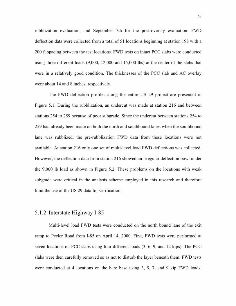
57
rubblization evaluation, and September 7th for the post-overlay evaluation. FWD
deflection data were collected from a total of 51 locations beginning at station 198 with a
200 ft spacing between the test locations. FWD tests on intact PCC slabs were conducted
using three different loads (9,000, 12,000 and 15,000 lbs) at the center of the slabs that
were in a relatively good condition. The thicknesses of the PCC slab and AC overlay
were about 14 and 8 inches, respectively.
The FWD deflection profiles along the entire US 29 project are presented in
Figure 5.1. During the rubblization, an undercut was made at station 216 and between
stations 254 to 259 because of poor subgrade. Since the undercut between stations 254 to
259 had already been made on both the north and southbound lanes when the southbound
lane was rubblized, the pre-rubblization FWD data from these locations were not
available. At station 216 only one set of multi-level load FWD deflections was collected.
However, the deflection data from station 216 showed an irregular deflection bowl under
the 9,000 lb load as shown in Figure 5.2. These problems on the locations with weak
subgrade were critical in the analysis scheme employed in this research and therefore
limit the use of the US 29 data for verification.
5.1.2 Interstate Highway I-85
Multi-level load FWD tests were conducted on the north bound lane of the exit
ramp to Peeler Road from I-85 on April 14, 2000. First, FWD tests were performed at
seven locations on PCC slabs using four different loads (3, 6, 9, and 12 kips). The PCC
slabs were then carefully removed so as not to disturb the layer beneath them. FWD tests
were conducted at 4 locations on the bare base using 3, 5, 7, and 9 kip FWD loads,
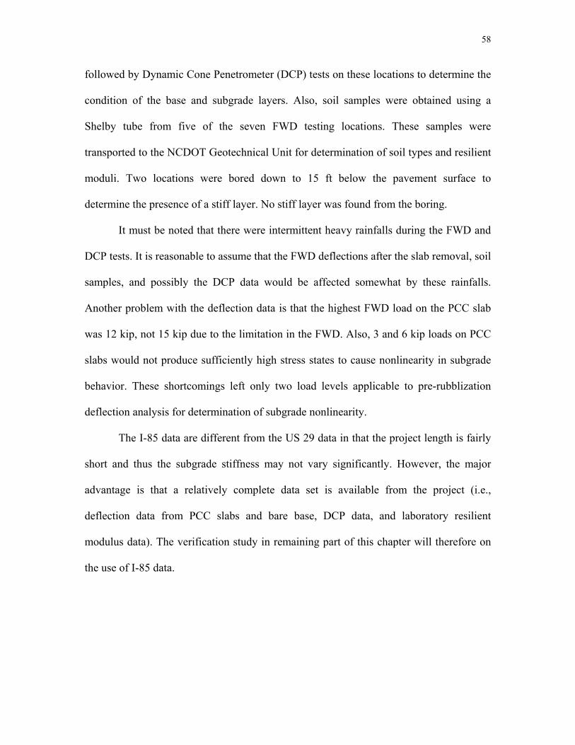
58
followed by Dynamic Cone Penetrometer (DCP) tests on these locations to determine the
condition of the base and subgrade layers. Also, soil samples were obtained using a
Shelby tube from five of the seven FWD testing locations. These samples were
transported to the NCDOT Geotechnical Unit for determination of soil types and resilient
moduli. Two locations were bored down to 15 ft below the pavement surface to
determine the presence of a stiff layer. No stiff layer was found from the boring.
It must be noted that there were intermittent heavy rainfalls during the FWD and
DCP tests. It is reasonable to assume that the FWD deflections after the slab removal, soil
samples, and possibly the DCP data would be affected somewhat by these rainfalls.
Another problem with the deflection data is that the highest FWD load on the PCC slab
was 12 kip, not 15 kip due to the limitation in the FWD. Also, 3 and 6 kip loads on PCC
slabs would not produce sufficiently high stress states to cause nonlinearity in subgrade
behavior. These shortcomings left only two load levels applicable to pre-rubblization
deflection analysis for determination of subgrade nonlinearity.
The I-85 data are different from the US 29 data in that the project length is fairly
short and thus the subgrade stiffness may not vary significantly. However, the major
advantage is that a relatively complete data set is available from the project (i.e.,
deflection data from PCC slabs and bare base, DCP data, and laboratory resilient
modulus data). The verification study in remaining part of this chapter will therefore on
the use of I-85 data.

59
0
2
4
6
8
10
12
198 218 238 258 278 298 318
Station Number (a)
Def
lect
ion
(mil)
9,000 lbs12,000 lbs15,000 lbs
0
1
2
3
4
5
198 218 238 258 278 298 318
Station Number (b)
Def
lect
ion
(mil)
9,000 lbs12,000 lbs15,000 lbs
UndercutLocations
UndercutLocations
Figure 5.1 Deflection profiles for US 29 before rubblization: (a) D0 and (b) D60
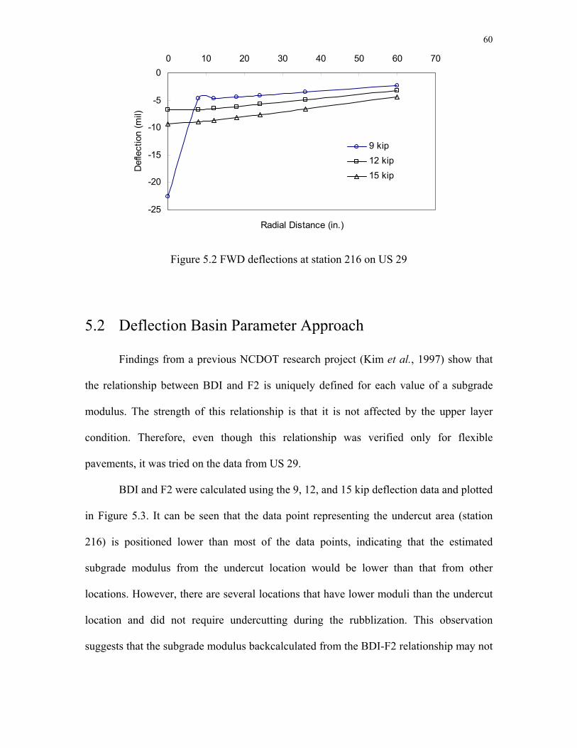
60
-25
-20
-15
-10
-5
00 10 20 30 40 50 60 70
Radial Distance (in.)
Def
lect
ion
(mil)
9 kip12 kip15 kip
Figure 5.2 FWD deflections at station 216 on US 29
5.2 Deflection Basin Parameter Approach
Findings from a previous NCDOT research project (Kim et al., 1997) show that
the relationship between BDI and F2 is uniquely defined for each value of a subgrade
modulus. The strength of this relationship is that it is not affected by the upper layer
condition. Therefore, even though this relationship was verified only for flexible
pavements, it was tried on the data from US 29.
BDI and F2 were calculated using the 9, 12, and 15 kip deflection data and plotted
in Figure 5.3. It can be seen that the data point representing the undercut area (station
216) is positioned lower than most of the data points, indicating that the estimated
subgrade modulus from the undercut location would be lower than that from other
locations. However, there are several locations that have lower moduli than the undercut
location and did not require undercutting during the rubblization. This observation
suggests that the subgrade modulus backcalculated from the BDI-F2 relationship may not
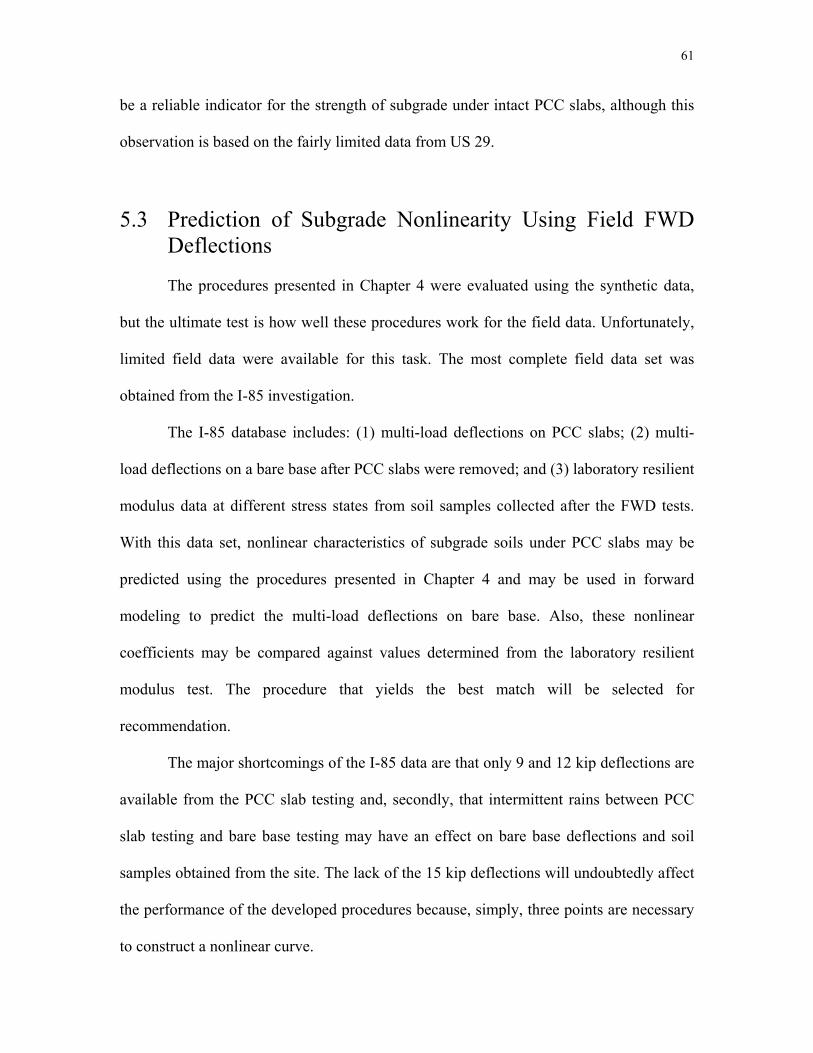
61
be a reliable indicator for the strength of subgrade under intact PCC slabs, although this
observation is based on the fairly limited data from US 29.
5.3 Prediction of Subgrade Nonlinearity Using Field FWD Deflections
The procedures presented in Chapter 4 were evaluated using the synthetic data,
but the ultimate test is how well these procedures work for the field data. Unfortunately,
limited field data were available for this task. The most complete field data set was
obtained from the I-85 investigation.
The I-85 database includes: (1) multi-load deflections on PCC slabs; (2) multi-
load deflections on a bare base after PCC slabs were removed; and (3) laboratory resilient
modulus data at different stress states from soil samples collected after the FWD tests.
With this data set, nonlinear characteristics of subgrade soils under PCC slabs may be
predicted using the procedures presented in Chapter 4 and may be used in forward
modeling to predict the multi-load deflections on bare base. Also, these nonlinear
coefficients may be compared against values determined from the laboratory resilient
modulus test. The procedure that yields the best match will be selected for
recommendation.
The major shortcomings of the I-85 data are that only 9 and 12 kip deflections are
available from the PCC slab testing and, secondly, that intermittent rains between PCC
slab testing and bare base testing may have an effect on bare base deflections and soil
samples obtained from the site. The lack of the 15 kip deflections will undoubtedly affect
the performance of the developed procedures because, simply, three points are necessary
to construct a nonlinear curve.
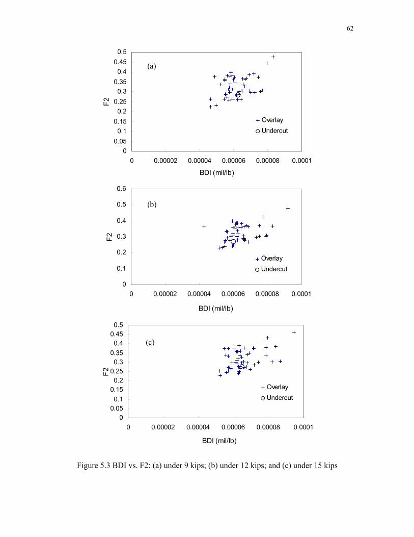
62
00.050.1
0.150.2
0.250.3
0.350.4
0.450.5
0 0.00002 0.00004 0.00006 0.00008 0.0001
BDI (mil/lb)
F2
OverlayUndercut
0
0.1
0.2
0.3
0.4
0.5
0.6
0 0.00002 0.00004 0.00006 0.00008 0.0001
BDI (mil/lb)
F2
OverlayUndercut
00.050.1
0.150.2
0.250.3
0.350.4
0.450.5
0 0.00002 0.00004 0.00006 0.00008 0.0001
BDI (mil/lb)
F2
OverlayUndercut
(a)
(c)
(b)
Figure 5.3 BDI vs. F2: (a) under 9 kips; (b) under 12 kips; and (c) under 15 kips

63
Four different approaches were tested using the field data: (1) direct prediction of
the nonlinear coefficients in the stress-based model (hereafter called the direct approach);
(2) a regression approach to predict the nonlinear coefficients in the stress-based model
(hereafter called the stress-based regression approach); (3) backcalculation of the stress-
based nonlinear coefficients using the genetic algorithm (hereafter called the GA
approach); and (4) the regression approach using the strain-based model (hereafter called
the strain-based regression approach). For the determination of the deflections from the
bare base, the nonlinear model used in backcalculation was used in forward finite element
modeling (i.e., the stress-based model for (1) to (3) and strain-based model for (4)). As
for the comparison with the laboratory-determined results, only the first three stress-
based methods are applicable because the laboratory resilient moduli were determined as
a function of stress states.
Since the deflections from only two load levels (9 and 12 kips) were available
from the PCC slab testing, the ANNs presented in Chapter 4 for the direct approach could
not be used. Instead, ANNs were retrained using only 9 and 12 kip data. Table 5.2
presents the RMSEs of training and testing cases for the retrained ANNs. The ANN
structures with bold numbers for RMSEs were selected as the optimum structures.
For the regression approaches using the stress and strain based models, stresses
and subgrade moduli at different locations on the subgrade were predicted for individual
load levels. Therefore, these approaches did not require retraining of the ANNs. For the
strain-based regression approach, Emax was predicted from the ANN trained based on 9
kip deflections. The ANN structures of 10-7-1 and 15-13-1 hidden layers in Table 4.14
were used in this field data analysis.

64
The GA technique was based on matching calculated deflection from a forward
model against measured deflections from field FWD tests with randomly changing
material properties (e.g., the PCC modulus and nonlinear coefficients of subgrade) until
the error becomes smaller than the tolerance. The calculated deflections were generated
by NCPAVE in the static mode using material properties randomly selected by the GA.
Generally, many cases of inputs should be tried to find the material properties
representing the field deflections. Finally, it was found that approximately 10 hours was
necessary to obtain the coefficients within the tolerance of 10% RMSE. This run time
makes the GA technique impractical for the DOT environment. More detailed
information on the GA technique is given in Appendix A.
The predicted nonlinear coefficients are shown in Table 5.3 for the direct,
regression, and GA approaches along with the laboratory-determined stress-based
coefficients. It can be observed from the table that ANN_1 and ANN_2 are not sensitive
enough to pick up the differences in the deflection basins between location A, B, and C.
Thus, ANN_1 and ANN_2 were dropped from the further analysis. For the stress-based
regression approach, the linearity was assumed for the deviator stress less than 0.5 psi.
All of the predicted deviator stresses under 9 and 12 kip loads were less than 0.5 psi in
location B. Therefore, the predicted nonlinear coefficients for location B are not available
in Table 5.3.
In order to find out the reason for the low deviator stress predicted from location
B, PCC modulus was investigated. From the NCHRP 10-48 study (Kim et al., 2000), it
was found that the surface layer modulus is a strong function of SCI. Equation (5.1) was

65
developed from the dynamic and nonlinear synthetic database using the regression
analysis (Figure 5.4):
890875.7)(*695362.1)(*131469.1)( +−−= HpccLogSCILogEpccLog
( 2R = 0.97) (5.1)
where
Epcc : PCC slab Young’s modulus,
SCI : – , and 0D 12D Hpcc : PCC slab thickness.
Table 5.2 Prediction accuracy of the direct backcalculation using different input units under 9 kip and 12 kip FWD loads
Input Hidden layer
Structure Output
Training Average
RMSE (%)
Testing Average
RMSE (%) 7-4-1 14.49 9.63 8-5-1 14.87 10.16 9-6-1
1k 13.48 10.99
7-4-1 22.10 15.87 8-5-1 26.68 17.29
ANN_1 D24, D36, D60, Hpcc
9-6-1 3k
18.17 13.61
13-10-1 9.66 9.16 14-11-1 9.86 8.38 15-12-1
1k 11.05 9.70
13-10-1 13.09 11.74 14-11-1 18.36 13.37
ANN_2 D0 to D60, Hpcc
15-12-1 3k
23.18 16.96
7-4-1 13.21 10.39 8-5-1 9.96 9.13 9-6-1
1k 12.16 9.69
7-4-1 23.91 19.49 8-5-1 18.19 16.88
ANN_3 AREA, D24,
D36, D60, Hpcc
9-6-1 3k
21.34 16.40
11-8-1 11.81 9.43 12-9-1 12.28 9.08
13-10-1 1k
11.97 9.00 11-8-1 17.06 11.64 12-9-1 17.73 13.85
ANN_4 BDI, F2, D24, D36, D60, Hpcc
13-10-1 3k
14.93 14.93
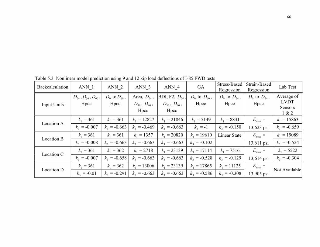
66
Table 5.3 Nonlinear model prediction using 9 and 12 kip load deflections of I-85 FWD tests
Backcalculation ANN_1 ANN_2 ANN_3 ANN_4 GA Stress-BasedRegression
Strain-BasedRegression Lab Test
Input Units 24D , , ,
Hpcc 36D 60D 0D to ,
Hpcc 60D Area, ,
D , , Hpcc
24D
60D36
BDI, F2, , D , D ,
Hpcc
24D
6036
0D to , Hpcc
60D 0D D to , Hpcc
24 0D D to , Hpcc
24 Average of LVDT Sensors 1 & 2
1k = 361 1k = 361 1k = 12827 1k = 21846 1k = 5149 1k = 8831 maxE = 1k = 15863 Location A
3k = -0.007 3k = -0.663 3k = -0.469 3k = -0.663 3k = -1 3k = -0.150 13,623 psi 3k = -0.659
1k = 361 1k = 361 1k = 1357 1k = 20820 1k = 19610 Linear State maxE = 1k = 19089 Location B
3k = -0.008 3k = -0.663 3k = -0.663 3k = -0.663 3k = -0.102 13,611 psi 3k = -0.524
1k = 361 1k = 362 1k = 2718 1k = 23139 1k = 17114 1k = 7516 maxE = 1k = 5522 Location C
3k = -0.007 3k = -0.658 3k = -0.663 3k = -0.663 3k = -0.528 3k = -0.129 13,614 psi 3k = -0.304
1k = 361 1k = 362 1k = 13006 1k = 23139 1k = 17865 1k = 11125 maxE = Location D
3k = -0.01 3k = -0.291 3k = -0.663 3k = -0.663 3k = -0.586 3k = -0.308 13,905 psi Not Available
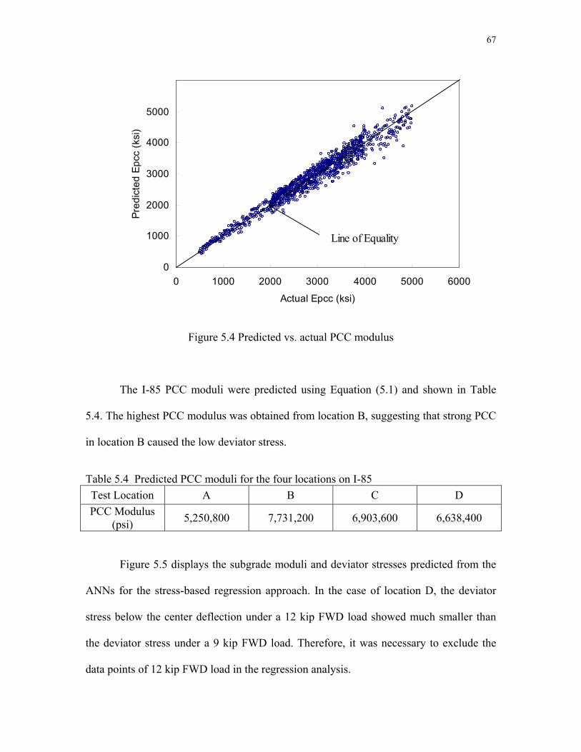
67
6000
0
1000
2000
3000
4000
5000
0 1000 2000 3000 4000 5000 6000
Actual Epcc (ksi)
Pred
icte
d Ep
cc (k
si)
Line of Equality
Figure 5.4 Predicted vs. actual PCC modulus
The I-85 PCC moduli were predicted using Equation (5.1) and shown in Table
5.4. The highest PCC modulus was obtained from location B, suggesting that strong PCC
in location B caused the low deviator stress.
Table 5.4 Predicted PCC moduli for the four locations on I-85 Test Location A B C D PCC Modulus
(psi) 5,250,800 7,731,200 6,903,600 6,638,400
Figure 5.5 displays the subgrade moduli and deviator stresses predicted from the
ANNs for the stress-based regression approach. In the case of location D, the deviator
stress below the center deflection under a 12 kip FWD load showed much smaller than
the deviator stress under a 9 kip FWD load. Therefore, it was necessary to exclude the
data points of 12 kip FWD load in the regression analysis.
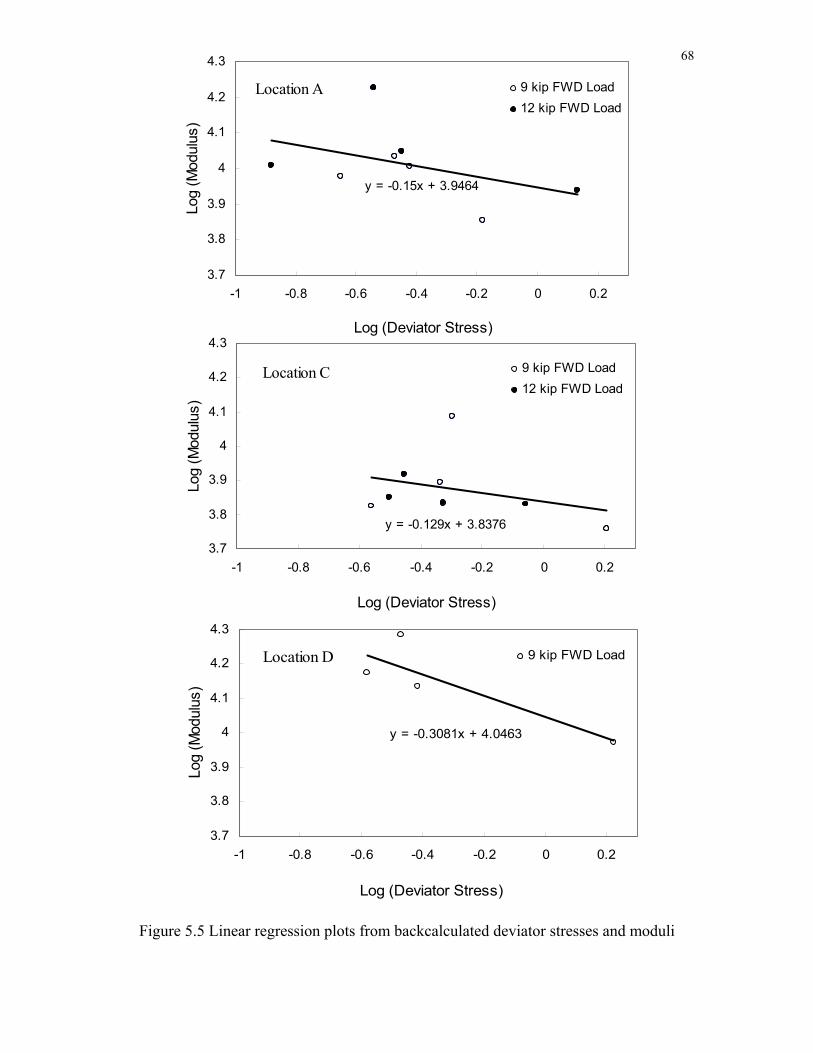
68
y = -0.15x + 3.9464
3.7
3.8
3.9
4
4.1
4.2
4.3
-1 -0.8 -0.6 -0.4 -0.2 0 0.2
Log (Deviator Stress)
Log
(Mod
ulus
)
9 kip FWD Load12 kip FWD Load
Location A
y = -0.129x + 3.8376
3.7
3.8
3.9
4
4.1
4.2
4.3
-1 -0.8 -0.6 -0.4 -0.2 0 0.2
Log (Deviator Stress)
Log
(Mod
ulus
)
9 kip FWD Load12 kip FWD Load
Location C
y = -0.3081x + 4.0463
3.7
3.8
3.9
4
4.1
4.2
4.3
-1 -0.8 -0.6 -0.4 -0.2 0 0.2
Log (Deviator Stress)
Log
(Mod
ulus
)
9 kip FWD LoadLocation D
Figure 5.5 Linear regression plots from backcalculated deviator stresses and moduli

69
5.4 Comparison between Measured and Calculated Deflections
In this section, the different approaches (ANN_3, ANN_4, stress-based
regression, GA, and strain-based regression) were tested to discern which one best
predicted subgrade conditions compared to the resilient modulus lab tests of the cored
soil materials. In addition, measured deflections under intact PCC slabs and bare base
FWD tests were compared with calculated deflections from forward models using
backcalculated nonlinear coefficients and Epcc. The backcalculated coefficients were
obtained from ANN_3, ANN_4, stress-based regression, GA, and strain-based regression
using FWD deflections under two load levels on PCC slabs, and the critical value of
in the strain-based regression was predicted from FWD deflections under a 9 kip load.
maxE
It needs to be noted that a discrepancy exists between the actual pavement
structure and the structure used in backcalculation. The I-85 pavement has a 5-inch thick
base layer, but it was necessary to neglect the base layer in the backcalculation because
the ANNs were trained for two-layer systems. To be more realistic in the forward
prediction, the base layer was included with a set of nonlinear coefficients estimated from
the DCP results and the visual observation of the base material during the FWD tests.
Figure 5.6 presents the CBR values at different depths estimated from the DCP
measurements at location A of I-85. The CBR value was converted from the penetration
depth measured from DCP tests according to the regression relationship in Figure 5.7.
The following equation is used by the NCDOT to convert the DCP reading into the CBR
value:
)(*076.1563.1)( DCPLogCBRLog −= (5.2)
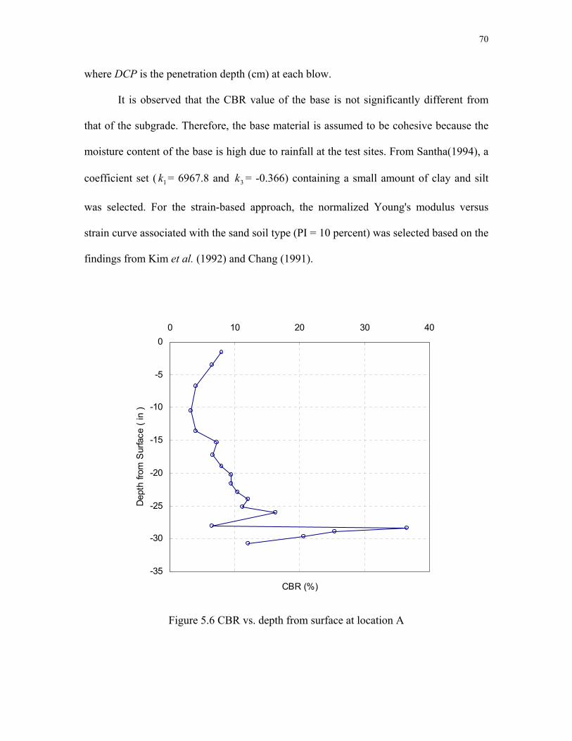
70
where DCP is the penetration depth (cm) at each blow.
It is observed that the CBR value of the base is not significantly different from
that of the subgrade. Therefore, the base material is assumed to be cohesive because the
moisture content of the base is high due to rainfall at the test sites. From Santha(1994), a
coefficient set ( = 6967.8 and k = -0.366) containing a small amount of clay and silt
was selected. For the strain-based approach, the normalized Young's modulus versus
strain curve associated with the sand soil type (PI = 10 percent) was selected based on the
findings from Kim et al. (1992) and Chang (1991).
1k 3
-35
-30
-25
-20
-15
-10
-5
00 10 20 30
CBR (%)
Dep
th fr
om S
urfa
ce (
in )
40
Figure 5.6 CBR vs. depth from surface at location A

71
Figure 5.7 The linear relationship curve between DCP reading and CBR
Figures 5.8 to 5.10 display the deflections measured from the field tests and
predicted from different backcalculation techniques. Generally, deflections predicted
from the ANN_4, stress-based regression, and lab tests show good agreement with the
measured deflections, considering the effects of narrowed stress distribution and rainfalls
during the tests.

72
Location A
-160
-140
-120
-100
-80
-60
-40
-20
00 20 40 60 80
Radial Distance (in)
Defle
ctio
n (m
il)
Field
ANN_4
GA
Lab
Stress-BasedReg.Strain-BasedReg.
Location B
-80
-70
-60
-50
-40
-30
-20
-10
00 20 40 60 80
Radial Distance (in)
Defle
ctio
n (m
il)
Field
ANN_4
GA
Lab
Strain-BasedReg.
Location C
-100
-90
-80
-70
-60
-50
-40
-30
-20
-10
00 20 40 60 80
Radial Distance (in)
Defle
ctio
n (m
il)
Field
ANN_4
GA
Lab
Stress-BasedReg.Strain-BasedReg.
-90
-80
-70
-60
-50
-40
-30
-20
-10
00 20 40 60 80
Radial Distance (in)
Defle
ctio
n (m
il)
Field
GA
Stress-BasedReg.Strain-BasedReg.
Location D
Figure 5.8 Comparison plot under 3 kip FWD load on bare base test

73
0 2
Location A
-350
-300
-250
-200
-150
-100
-50
00 20 40 60 80
Radial Distance (in)
Defle
ctio
n (m
il)
Field
ANN_4
GA
Lab
Stress-Based Reg.Strain-BasedReg.
Location B
-180
-160
-140
-120
-100
-80
-60
-40
-20
00 20 40 60 8
Radial Distance (in)
Defle
ctio
n (m
il)
Field
ANN_4
GA
Lab
Strain-BasedReg.
Location C
-250
-200
-150
-100
-50
00 40 60 80
Radial Distance (in)
Defle
ctio
n (m
il) Field
ANN_4
GA
Lab
Stress-BasedReg.Strain-BasedReg.
-250
-200
-150
-100
-50
00 20 40 60 8
Radial Distance (in)
Defle
ctio
n (m
il)
Field
ANN_4
GA
Stress-BasedReg.Strain-BasedReg.
Location D
0
0
Figure 5.9 Comparison plot under 5 kip FWD load on bare base test
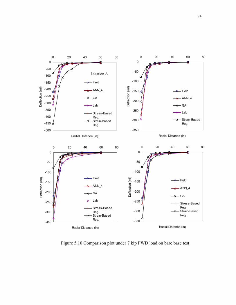
74
-500
-450
-400
-350
-300
-250
-200
-150
-100
-50
00 20 40 60 80
Radial Distance (in)
Defle
ctio
n (m
il)
Field
ANN_4
GA
Lab
Stress-BasedReg.Strain-BasedReg.
Location A
-350
-300
-250
-200
-150
-100
-50
00 20 40 60 8
Radial Distance (in)
Defle
ctio
n (m
il)
Field
ANN_4
GA
Lab
Strain-BasedReg.
-350
-300
-250
-200
-150
-100
-50
00 20 40 60 80
Radial Distance (in)
Defle
ctio
n (m
il) Field
ANN_4
GA
Lab
Stress-BasedReg.Strain-BasedReg. -350
-300
-250
-200
-150
-100
-50
00 20 40 60 8
Radial Distance (in)
Defle
ctio
n (m
il)
Field
ANN_4
GA
Stress-BasedReg.Strain-BasedReg.
0
0
Figure 5.10 Comparison plot under 7 kip FWD load on bare base test
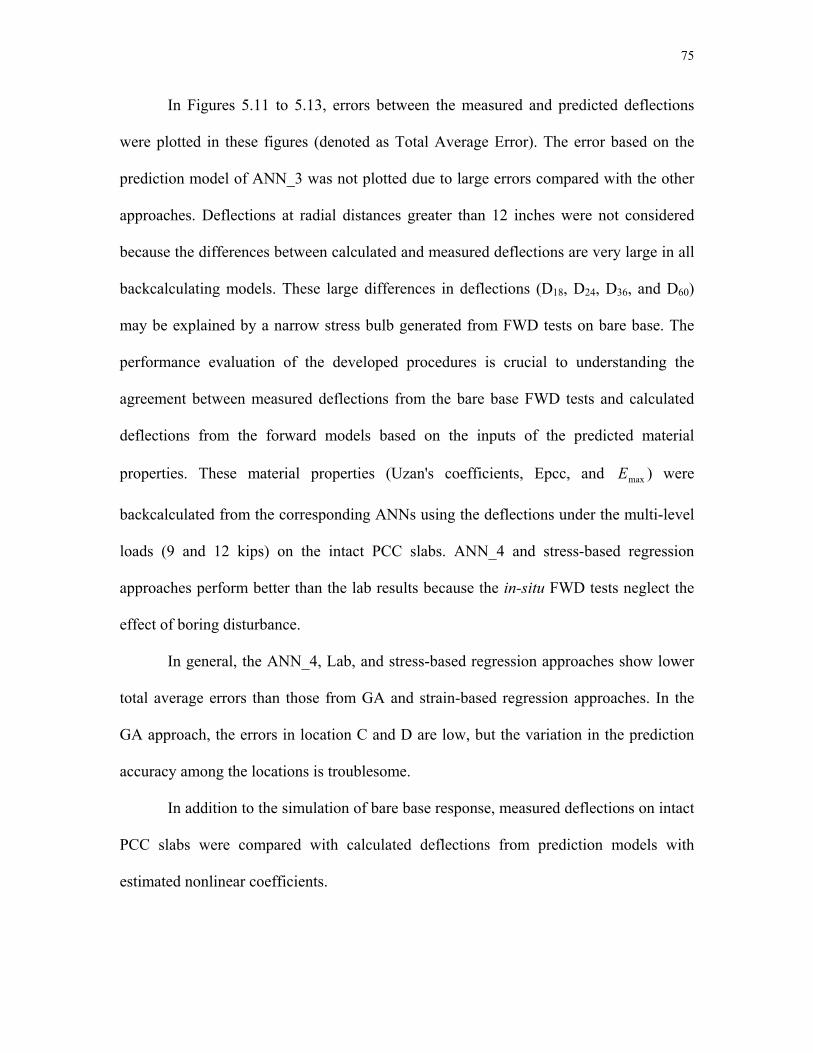
75
In Figures 5.11 to 5.13, errors between the measured and predicted deflections
were plotted in these figures (denoted as Total Average Error). The error based on the
prediction model of ANN_3 was not plotted due to large errors compared with the other
approaches. Deflections at radial distances greater than 12 inches were not considered
because the differences between calculated and measured deflections are very large in all
backcalculating models. These large differences in deflections (D18, D24, D36, and D60)
may be explained by a narrow stress bulb generated from FWD tests on bare base. The
performance evaluation of the developed procedures is crucial to understanding the
agreement between measured deflections from the bare base FWD tests and calculated
deflections from the forward models based on the inputs of the predicted material
properties. These material properties (Uzan's coefficients, Epcc, and ) were
backcalculated from the corresponding ANNs using the deflections under the multi-level
loads (9 and 12 kips) on the intact PCC slabs. ANN_4 and stress-based regression
approaches perform better than the lab results because the in-situ FWD tests neglect the
effect of boring disturbance.
maxE
In general, the ANN_4, Lab, and stress-based regression approaches show lower
total average errors than those from GA and strain-based regression approaches. In the
GA approach, the errors in location C and D are low, but the variation in the prediction
accuracy among the locations is troublesome.
In addition to the simulation of bare base response, measured deflections on intact
PCC slabs were compared with calculated deflections from prediction models with
estimated nonlinear coefficients.

76
Tota
l Ave
rage
Err
or (%
)
Strain- Based Reg.
Lab Stress- Based Reg.
GA ANN_4
Figure 5.11 Absolute errors between calculated and measured deflections under 3 kip FWD load on bare base
Tota
l Ave
rage
Err
or (%
)
Stress- Based Reg.
Strain- Based Reg.
ANN_4 GA Lab
Figure 5.12 Absolute errors between calculated and measured deflections under 5 kip FWD load on bare base
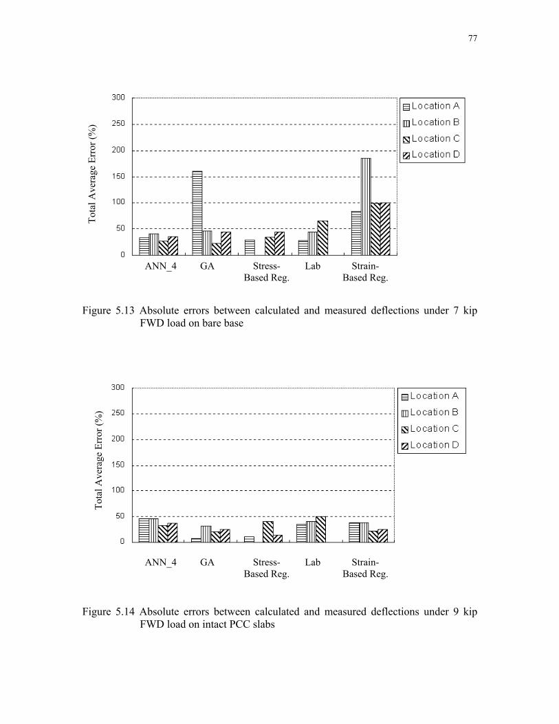
77
Tota
l Ave
rage
Err
or (%
)
Strain- Based Reg.
Lab Stress- Based Reg.
GA ANN_4
Figure 5.13 Absolute errors between calculated and measured deflections under 7 kip FWD load on bare base
Tota
l Ave
rage
Err
or (%
)
Strain- Based Reg.
Lab Stress- Based Reg.
GA ANN_4
Figure 5.14 Absolute errors between calculated and measured deflections under 9 kip
FWD load on intact PCC slabs
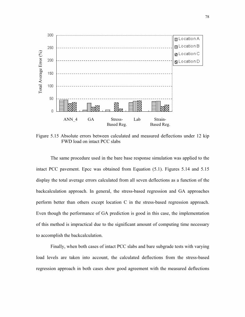
78
Tota
l Ave
rage
Err
or (%
)
Stress- Based Reg.
Strain- Based Reg.
ANN_4 GA Lab
Figure 5.15 Absolute errors between calculated and measured deflections under 12 kip FWD load on intact PCC slabs
The same procedure used in the bare base response simulation was applied to the
intact PCC pavement. Epcc was obtained from Equation (5.1). Figures 5.14 and 5.15
display the total average errors calculated from all seven deflections as a function of the
backcalculation approach. In general, the stress-based regression and GA approaches
perform better than others except location C in the stress-based regression approach.
Even though the performance of GA prediction is good in this case, the implementation
of this method is impractical due to the significant amount of computing time necessary
to accomplish the backcalculation.
Finally, when both cases of intact PCC slabs and bare subgrade tests with varying
load levels are taken into account, the calculated deflections from the stress-based
regression approach in both cases show good agreement with the measured deflections

79
from the field tests. Based on this observation, the stress-based regression approach will
be implemented to develop a backcalculation program for PCC pavements.
5.5 Recommended Procedure
The following steps are recommended to determine whether the subgrade in
question is strong enough to handle a construction equipment during rubblization:
Step 1 : Conduct FWD tests at the center of intact PCC slabs using multi-level loads (9,
12, and 15 kips). To minimize the effect of warping, these tests should be
performed at the earliest time in the morning.
Step 2 : Calculate the deviator stresses and moduli in subgrade at radial distance of 0, 8,
12, and 24 inches using the ANN backcalculation program.
Step 3 : Run the power regression analysis (or linear regression when logarithmic values
are used) between the deviator stresses and subgrade moduli.
Step 4 : Calculate the maximum deflection caused by an equipment in question using
NCPAVE-static. The input values are the predicted coefficients of the stress-
based regression, the surface layer thickness, and a typical rubblized modulus of
500 ksi.
Step 5 : Determine whether the maximum deflection will cause the problems during
rubblization.
80
CHAPTER SIX CONCLUSIONS AND RECOMMENDATIONS
FOR FUTURE RESEARCH
6.1 Conclusions
In this research, the nonlinear subgrade condition was investigated using multi-
level FWD loads on intact PCC slabs. Both the stress and strain-based models were
studied to represent the subgrade nonlinearity. The nonlinear coefficients in these models
were determined either by presenting them directly from ANNs or by running regression
analysis between stresses (or strains) and subgrade moduli predicted from surface
deflections. The performance of these approaches was evaluated using the data from I-85.
The following conclusions may be drawn from this investigation:
1. The nonlinearity of subgrade is important to estimate subgrade responses, such as
stresses and strains, under multi-level FWD loads. The study shows that deviator
stresses calculated from the nonlinear analysis are generally larger than those from the
linear analysis. That is, the linear analysis could underestimate the subgrade response.
2. In general, stresses and strains in subgrade are easier to be predicted from deflection
using ANNs than nonlinear material properties. Additionally, the investigation shows
that in -situ FWD tests are better than destructive coring and lab test approaches.
3. Results from this study confirm that the highest FWD load on a thick and/or strong
layer cannot cause nonlinear behavior in subgrade. When the predicted stress in
subgrade is less than 0.5 psi, coring followed by DCP testing is recommended for
subgrade stiffness evaluation.
81
4. Based on very limited field data from I-85, the stress-based regression approach seems
to be most promising.
6.2 Recommendations for Future Research
This research has resulted in a significant amount of information regarding the
subgrade nonlinearity under multi-level FWD loads. Several procedures of predicting
subgrade nonlinearity under intact PCC slabs have been developed in this research using
the dynamic and nonlinear synthetic database. However, the complexity involved in the
nonlinear analysis requires the verification of these procedures using field data.
Only very limited data were available for this purpose during the research. It is
strongly recommended to verify these procedures using additional field data in the future.
The additional verification effort will require: (1) deflections measured on PCC slabs
using 9, 12, and 15 kip loads; (2) deflections measured on bare subgrade using 3, 5, and 7
kip loads; (3) DCP readings; and (4) laboratory resilient moduli values of soil samples.
With this additional work, a reliable backcalculation program for PCC pavement can be
developed that will aid not only rubblization decisions but also the overlay thickness
design after rubblization.
82
LIST OF REFERENCES
AASHTO. (1993). AASHTO Guide for Design of Pavement Structures. Amer. Assoc. of
State Highway and Trans. Officials.
Borden, R. H., Shao, L., and Gupta, A. (1994). “Construction Related Vibrations.”
FHWA/NC Report 94-007, Center for Transportation Engineering Studies, North
Carolina State University.
Brown, S. F. and Pappin, J.W., (1981), “Analysis of Pavements with Granular Bases.”
Transportation Research Record, No. 810, pp. 17-23.
Brown, S. F., Louch, S. C., and O’Reilly, M. P. (1987). “Repeated Loaded Loading of
Fine Grained Soils.” TRRL Contractors Report, CR72, School of Civil Engineering,
University of Nottingham, Nottingham, England.
Chang, D. (1991). Nonlinear Effects on Dynamic Response of Pavements Using the
Nondestructive Testing Techniques. Dissertation, UT at Austin.
Corley-Lay, Judith. (1996). NCDOT correspondence on I-85 Rubblization Project.
Corley-Lay, Judith. (1997). State Pavement Analysis Engineer. NCDOT. Personal
interview.
Corley-Lay, Judith B., Thomas M. Hearne, and Shie-Shin Wu. (1995). “Deflection Study
and Design of Crack and Seat Pavement Rehabilitation.” Transportation Research
Record, No. 1513.
Daleiden, Jerome F., David A. Ooten, and Mark D. Sargent. (1995). “Rehabilitation of a
Jointed Portland Cement Concrete Pavement on I-35 (Southbound) in Kay County,
Oklahoma.” Transportation Research Record, No. 1513, pp. 61-69.

83
Dayhoff, J. (1990). Neural Network Architectures: An Introduction. Van Nostrand
Reinhold, New York.
Desai, C. S., and H. J. Siriwardane. (1984). Constitutive Laws for Engineering Materials.
Prentice-Hall, Inc., Englewood Cliffs, NJ.
Ellacott, S., D. Bose. (1996). Neural Networks. Deterministic Methods of Analysis, ITP,
London.
Elliot, R. P., and David, L. (1989). “Improved Characterization Model for Granular
Bases.” Transportation Research Record, No. 1227, pp. 128-133.
Filho, J. R., C. Alippi, and P. Treleaven. (1994). “Genetic Algorithm Programming
Environments. ” IEEE Computer Journal, Vol. 27, pp 28-48.
Fredlund, D. G., A. T. Bergan, and P.K. Wong. (1977). “Relation Between Resilient
Modulus and Stress Condition for Cohesive Subgrade Soils.” Transportation
Research Record, No. 642, pp. 73-81.
Garg, N., and Thomson, M. R. (1997). “Triaxial Characterization of Mn/ROAD Granular
Materials.” Paper presented at 76th Annual Transportation Research Board Meeting,
January.
Garson, G. D. (1998). Neural Networks, An Introductory Guide for Social Scientists.
SAGE Publications, London.
Goldberg, D. E. (1989). Genetic Algorithms in Search, Optimization and Machine
Learning. Addison-Wesley, Reading, Mass.

84
Hall, K. T. and M. I. Darter. (1994). “Improved Methods for Asphalt-Overlaid Concrete
Pavement Backcalculation and Evaluation.” Nondestructive Testing of Pavements
and Backcalculation of Moduli. 2nd Volume, STP 1198, ASTM, pp. 83-102.
Haykn, S. (1994). Neural Networks. Macmillan College Publishing Company, New
York.
Hecht-Nielsen, R. (1990). Neurocomputing. Addision-Wesley. Reading, Mass.
Holland, J. H. (1975). Adaptation in Natural and Artificial Systems. University of
Michigan Press, Ann Arbor.
Hylton, J. M. (1997). Rehabilitation of Aging PCC Pavement Using Rubblization
Techniques. Technical Report, North Carolina State University.
Huang, Y. H. (1993). Pavement Analysis and Design. Prentice-Hall, Inc. Englewood
Cliffs, New Jersey.
Iannides, A. M. (1994). “Concrete Pavement Backcalculation Using ILL-BACK 3.0.”
Nondestructive Testing of Pavements and Backcalculation of Moduli. 2nd Volume,
STP 1198, ASTM, pp. 103-124.
Kim, D. S., and K. H. Stokoe II. (1992). “Characterization of Resilient Modulus of
Compacted Subgrade Soils Using Resonant Column and Torsional Shear Tests.”
Transportation Research Record, No. 1369, pp.83-91.
Kim, Y. (1997). In -Situ Evaluation of Microcrack Damage and Healing of Asphalt
Concrete Pavements Using Stress Wave Test. Dissertation, North Carolina State
University.

85
Kim, Y. R., J. D. Ranjithan, J.D. Troxler, and B. Xu (2000). “Assessing Pavement Layer
Condition Using Deflection Data.” Final Report, NCHRP 10-48.
Kim, Y. R. and Y-C. Lee. (1997). “Condition Assessment of Flexible Pavements Using
FWD Deflections.” Final Report, NCDOT Project.
Kuennen, Tom. (1991). “Resonant ‘rubblizing’ puts asphalt over concrete.” Roads and
Bridges. Jan., p. 50.
Kuo, C-M., K. T. Hall, and M. I. Darter. (1995). “Three-Dimensional Finite Element
Model for Analysis of Concrete Pavement Support.” Transportation Research Record,
No. 1505, pp. 26-32.
Lee, Y-C. (1997). Condtion Assessment of Flexible Pavements Using FWD Deflections.
Dissertation, North Carolina State University.
Mallela, J., and K. P. George. (1994). “Three-Dimensional Dynamic Respons Model for
Rigid Pavements. ” Transportation Research Record, No. 1448, pp. 92-99.
May, R. W., and Witczak, M. W. (1981). “Effective Granular Modulus to Model
Pavement Responses.” Transportation Research Record, No. 810, pp. 1-9.
Michalewicz, Z. (1999). Genetic Algorithms + Data Structures = Evolution Programs.
Springer-Verlag Berlin Heidelberg, New York.
NCHRP. (1996). “Laboratory Determination of Resilient Modulus for Flexible Pavement
Design.” National Cooperative Highway Research Board, pp.75-82.
Nelson, Thomas B., and Sam Owusu-Ababio. (1994). Preliminary Report - Research
Study #93-06: Investigation of the Performance of Fractured Slab Techniques for
PCC Pavements. Report for Wisconsin DOT, Oct.
86
Niederquell, M. G., G. Y. Baladi, and K. Chatti. (2000). “Rubblization of Concrete
Pavements Field Investigation.” Transportation Research Board, 79th Annual
Meeting, January 9-13, Washington, D.C.
PCS. (1991). Pavement Consultancy Services. Guidelines and Methodologies for the
Rehabilitation of Rigid Highway Pavements using Asphalt Concrete Overlays. Report
for NAPA and SAPAE, June.
Pezo, R. F. (1993). “A general Method of Reporting Resilient Modulus of Tests of Soils,
A Pavement Engineer’s Point of View.” Paper presented at 72nd Annual
Transportation Research Board Meeting, January.
Santha, B. L. (1994). “Resilient Modulus of Subgrade Soils: Comparison of Two
Constitiutive Equations. ” Transportation Research Board, No. 1462, pp. 79-90.
Schackner, Bill. (1989). “Rubble rebuilds roads.” The Times Union, Jan., B.
Thadkamalla, G. B., and George, K. P. (1995). “Characterization of Subgrade Soils at
Simulated Field Moisture.” Transportation Research Record, No. 1481, pp.21-27.
Thompson, M. R. (1999). “Hot Mix Asphalt Overlay Design Concepts for Rubblized
PCC Pavements. ” Transportation Research Board, 78th Annual Meeting, January 10-
14, Washington, D.C.
Thompson, M. R., and Elliot, R. P. (1985). “ILLI-PAVE-Based Response Algorithms for
Design of Conventional Flexible Pavements.” Transportation Research Record, No.
1043, pp. 55-57.
Tutumluer, Erol, and Thompson, M. R. (1997). “Anisotropic Modeling of Granular Bases
in Flexible Pavements.” Paper presented at 76th Annual Transportation Research
Board Meeting, January.

87
Uddin, W., R. B. Hackett, A. Joseph, Z. Pan, and A. B. Crawley. (1995). “Three-
Dimensional Finite Element Analysis of Jointed Concrete Pavement with
Discontinuities.” Transportation Research Record, No. 1482, pp. 26-32.
Ullidtz, P. (1998). Modelling Flexible Pavement Response and Performance. Narayana
Press, Gylling, Denmark.
Uzan, J. (1985). “Characterization of Granular Materials.” Transportation Research
Record, No. 1022, pp. 52-59.
Uzan, J., R. Briggs, and T. Scullion. (1992). “Backcalculation of Design Parameters for
Rigid Pavements. ” Transportation Research Record, No. 1377, pp. 107-114.
Waller, Fred. “Rubblizing the Raleigh Beltline.” Asphalt: 8-9.
Wasserman, P. D. (1993). Advanced Methods in Neural Computing. Van Nostrand
Reinhold, New York, 1993
Witczak M. W., and J. Uzan. (1988). “Universal Airport Pavement Design System. ”
Report I of IV , Granular Material Characterization, University of Maryland.
Yoder, E. J., and M. W. Witczak. (1975). Principles of Pavement Design. 2nd Ed. John
Wiley & Sons, Inc., New York.
Zaghloul, S. M., and T. D. White. (1993). “Use of a Three-Dimensional, Dynamic Finite
Element program for Analysis of Flexible Pavement.” Transportation Research
Record, No. 1388, pp. 60-69.

88
APPENDIX A ESTIMATION OF LAYER CONDITION
One of the most important objectives in FWD testing is the estimation of pavement
layer condition. To accomplish this objective, the following three elements must be present
in the FWD testing and analysis:
(1) FWD testing with proper load levels and sensor spacings;
(2) formulation of a theoretical input-response relationship (that is, a forward model) from
an idealized model which incorporates various parameters of assumed constitutive
models for the multiple layers in the pavement system; and
(2) identification of the system parameters (that is, inversion or backcalculation) by
matching in-situ measurements of responses and calculated responses from theoretical
input-response relationships.
To accomplish the objective of this research, FWD testing with 9, 12, and 15 kip
loads and sensor spacings of 8, 12, 18, 24, 36, and 60 inches was conducted. Also, a
dynamic axisymmetric finite element analysis with Uzan’s stress-state dependent model
for subgrade was identified as an appropriate forward model. To identify the most
suitable backcalculation method, various inversion techniques were examed in this
research. These techniques may be categorized into the following four groups:
(1) optimization techniques in which layer moduli and thicknesses are searched
(backcalculated) on the basis of error minimization strategies, such as conjugate
gradient, Newton’s method, and generic algorithm;
(2) data base inversion programs (e.g., MODULUS) that compare deflections with a pre-
generated database to determine layer properties using interpolation;
89
(3) closed-form methods (Ioannides, 1994) in which a unique relationship between the
deflection basin and the radius of relative stiffness is regressed to backcalculate the
subgrade stiffnesses from the deflection basin parameters; and
(4) artificial neural networks in which input-output relationships are trained from a large
database.
The following sections present those backcalculation techniques that are considered
candidates in this research.
A.1 Existing Backcalculation Methods for Rigid Pavement
A.1.1 Theoretical Models for Backcalculation
In this section, three types of models are presented for evaluating the material
parameters in the rigid pavement. These models have linear load-deformation
characteristics and cannot represent any nonlinear material behavior or discontinuity
between each layer. Most PCC forward models have been developed based on these
theoretical models when PCC pavement structures are assessed. Some modified
programs consider PCC slab curling effect due to temperature cycling.
A.1.1.1 Hertz-Westerggard Model
In this model a concrete slab rests on a dense liquid foundation, which is
composed of an infinite number of springs. The total volume of displacement of the
foundation is proportional to the total applied load. Based on this relationship, the
modulus of subgrade reaction and the radius of relative stiffness in the slab-subgrade
system may be determined. Since the vertical force at a given spring depends only on the

90
vertical deflection at that spring and is independent of the deflections at all other points,
the liquid foundation does not simulate the actual field condition.
A.1.1.2 Hogg Model
The Hogg model represents the pavement with infinite concrete slab resting on an
elastic foundation. An elastic foundation behaves more realistically than a liquid
foundation because the deflection depends not only on the force at a given point but also
on the forces at all points. (Huang, 1993). This type of foundation is also called a
Boussinesq foundation because the Boussinesq equation for surface deflection is used for
determining the stiffness matrix. In this model, the pavement parameters are the subgrade
modulus of elasticity and the radius of relative stiffness of the slab-subgrade system. The
load-deflection relationship is defined as follows:
jif
fjji dE
vPw
,
2
,
)1(π
−= (A.1)
where
w = deflection at given node,
P = force at given node,
Ef = elastic modulus of foundation,
d = distance of nodes, and
fν = Poisson’s ratio of foundation.

91
A.1.1.3 Multi-layered Elastic Model
This model, usually used in flexible pavement, assumes Hooke’s model to
characterize the linear elastic layers. The linear elastic layers extend to infinity in the
horizontal direction.
A.2.1 Backcalculation Procedures
A.2.1.1 JUSLAB Procedures
The JUSLAB, proposed by Uzan et al. (1992), is the one method used to
determine the material parameters using FWD deflection data in the rigid pavement. This
backcalculation procedure of layer properties for rigid pavement follows the MODULUS
backcalculation framework. The outputs are the set of layer moduli that minimize the
error between measured and theoretical calculated deflection bowls.
(1) A linear elastic computer program is run for a range of layer moduli, and the resulting
deflections are stored in a deflection database.
(2) Pattern search and interpolation schemes are used to minimize the error between
measured and theoretically calculated deflection bowls.
In order to minimize error, a pattern search routine to find the layer moduli uses an
objective function as follows:
( ) 2
1min∑ =
−N
imi
cimi
DDD
(A.2)
where
Dm = the measured deflection,
Dc = the calculated deflection, and
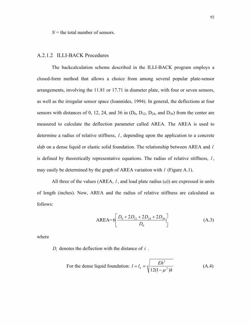
92
N = the total number of sensors.
A.2.1.2 ILLI-BACK Procedures
The backcalculation scheme described in the ILLI-BACK program employs a
closed-form method that allows a choice from among several popular plate-sensor
arrangements, involving the 11.81 or 17.71 in diameter plate, with four or seven sensors,
as well as the irregular sensor space (Ioannides, 1994). In general, the deflections at four
sensors with distances of 0, 12, 24, and 36 in (D0, D12, D24, and D36) from the center are
measured to calculate the deflection parameter called AREA. The AREA is used to
determine a radius of relative stiffness, l , depending upon the application to a concrete
slab on a dense liquid or elastic solid foundation. The relationship between AREA and l
is defined by theoretically representative equations. The radius of relative stiffness, l ,
may easily be determined by the graph of AREA variation with (Figure A.1). l
All three of the values (AREA, , and load plate radius (a)) are expressed in units
of length (inches). Now, AREA and the radius of relative stiffness are calculated as
follows:
l
AREA=
+++
0
3624120 222D
DDDD6 (A.3)
where
iD denotes the deflection with the distance of . i
For the dense liquid foundation: 42
3
)1(12 kEhlk µ−
==l (A.4)
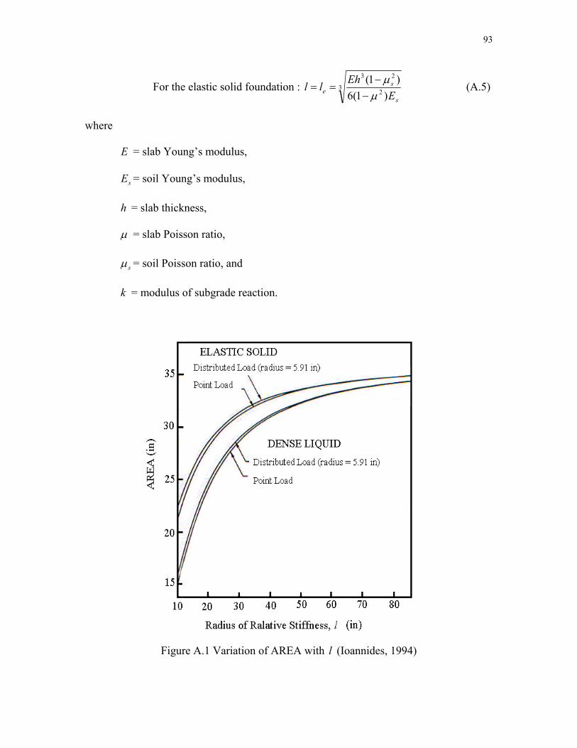
93
For the elastic solid foundation : 32
23
)1(6)1(
s
se E
Ehllµ
µ−
−== (A.5)
where
E = slab Young’s modulus,
sE = soil Young’s modulus,
h = slab thickness,
µ = slab Poisson ratio,
sµ = soil Poisson ratio, and
k = modulus of subgrade reaction.
Figure A.1 Variation of AREA with (Ioannides, 1994) l

94
As seen in Equation A.4, the dense liquid foundation cannot be applied when
determining a subgrade modulus. Therefore, the backcalculation procedure using the
elastic solid foundation model must be explained in detail. For elastic solid foundations,
nondimensional deflections ( ) can be expressed as id
==
laf
PlDDd i
ii 2 (A.6)
where
iD = deflection with the distance of i ,
a = radius of load plate, and
D is the slab flexural stiffness, which is given by :
)1(12 2
3
µ−=
EhD (A.7)
According to studies (Ioannides, 1984; 1988), the nondimensional deflections, can all
be written as functions of (
id
la ) only. The functional form of )(0 l
af is provided by
Losberg’s solution for the deflection at the center of the load.
−−= )]ln(010340141335.0[)(1
331)( 2
la
la
lafo (A.8)
Curve-fitting techniques were used in the ILLI-BACK program to obtain the regression
equation for
lafi (for =1, … , n). From the known load plate radius, a, the i
95
nondimensional deflection may be obtained by the regression equation or a relationship
graph between nondimensional deflections and radius of relative stiffness. Therefore, the
foundation elastic subgrade modulus can be backcalculated from Equations 4.5 to 4.7 as
follows:
lP
DdE
i
iss
2)1( 2µ−= (A.9)
Additionally, the slab flexural stiffness and the slab modulus can be calculated and
expressed respectively as:
22
3
)1(12Pl
DdEhD
i
i=−
=µ
(A.10)
23
2 )1(12 PlDd
hE
i
iµ−= (A.11)
On the basis of the fundamental concept above, the backcalculation procedure
may be applied along the following steps:
(1) Carry out FWD tests, and record the applied load as well as the measured deflections.
(2) Calculate the deflection parameter called AREA.
(3) Determine the radius of relative stiffness, , using the calculated AREA from the
relationship curve.
l
(4) Determine the nondimensional deflection with the value from a graph showing the
relationship between and d .
l
l i
(5) Based on l and , compute , , and id sE D E .
96
A.2.1.3 RMODS Program
Uzan et al. (1992) developed RMODS (rigid pavement evaluation and
backcalculation system) that is based on the pattern search technique for matching the
measured deflection basin with a theoretically calculated deflection basin. The procedure
for backcalculating the pavement parameters is similar to MODULUS for evaluating
flexible pavements. RMODS analyzes deflection basins with the corresponding
theoretical forward model as follows:
(1) For the edge deflection basins, only the Westergaard model is used since all other
models are not applicable.
(2) For center slab deflection basins, either the Hertz or the multi-layer elastic models is
used.
A.3 Base Damage Index and Shape Factor F2
Kim et al. (1997) investigated relationships among deflection basin parameters,
layer moduli, and layer thicknesses. They found that the relationship between Base
Damage Index (BDI) and Shape Factor F2 is uniquely defined for each value of and
is independent of upper layers’ moduli and thicknesses. The BDI and F2 are defined as:
sgE
2412 DDBDI −= (A.12)
24
36122D
DDF −= (A.13)
where
BDI = Base Damage Index (mil),
F2 = Shape Factor (dimensionless),
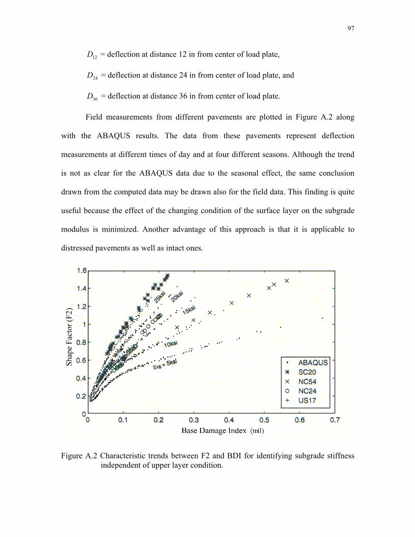
97
12D = deflection at distance 12 in from center of load plate,
24D = deflection at distance 24 in from center of load plate, and
36D = deflection at distance 36 in from center of load plate.
Field measurements from different pavements are plotted in Figure A.2 along
with the ABAQUS results. The data from these pavements represent deflection
measurements at different times of day and at four different seasons. Although the trend
is not as clear for the ABAQUS data due to the seasonal effect, the same conclusion
drawn from the computed data may be drawn also for the field data. This finding is quite
useful because the effect of the changing condition of the surface layer on the subgrade
modulus is minimized. Another advantage of this approach is that it is applicable to
distressed pavements as well as intact ones.
Figure A.2 Characteristic trends between F2 and BDI for identifying subgrade stiffness independent of upper layer condition.

98
A.4 Artificial Neural Networks
Artificial neural networks are a computational paradigm completely different
from conventional serial computing. Instead of the linear sequence of relatively complex
tasks that typifies most mathematical algorithms, artificial neural networks process
information in parallel using a large number of operationally simple but highly
interconnected processing units. The processing units have certain functional similarities
to biological neurons, and their organization bears resemblance to the organization of
neurons in the brain (Wasserman, 1993).
A neural network is a massively parallel distributed processor that has a natural
tendency for storing experiential knowledge and making it available for use. It resembles
the brain in two respects:
(1) Knowledge is acquired by the network through a learning process.
(2) Inter-neuron connection strengths, known as synaptic weights, are used to store the
knowledge (Haykin, 1994).
Neural network approaches are inspired, therefore, by biological neural networks.
It is generally understood that all biological neural functions, including memory, are
stored in the neurons and in the connections between them during a learning process. As
Figure A.3 illustrates, in biological neural networks dendrites collect signals which they
feed to the neuron. The neuron, in turn, processes the signals by sending a spike of
electrical current along an axon, discharging it at a synapse connecting it to other
neurons, which in turn are excited or inhibited as a result. In an artificial neural network,
input signals are sent to a neural processing entity, also called a neuron. After processing,
the neuron sends an output signal on to other neurons in the network (Garson, 1998).

99
Therefore, a neural network is a parallel distributed processing system composed
of processing entities (generally called neurons or units) that are interconnected to form a
mathematical representation of the mapping or relationship that may be embedded in any
set of data. The structure of ANNs allows the processing entities to be global
approximators even in the absence of knowledge about the mathematical form of the
mapping between an input signal and the corresponding output signal. A multi-layer
feedforward network is the most common class of ANNs used for this type of function
mapping (Dayhoff, 1990).
Figure A.3 Biological and neural networks
A typical multilayered network is characterized by the presence of one or more
hidden layers, whose computation nodes are correspondingly called hidden units or

100
hidden neurons (Figure A.4). The function of the hidden units is to intervene between the
external input and the network output (Haykin, 1994). The input signal is presented to the
network through the units in the input layer. This signal is then propagated through the
hidden units to the output units via the interconnections in the network. The strength of
the propagated signal is adjusted throughout the network by the connection strengths,
generally called weights. These weights are updated, in an iterative manner, until the
predicted output signals are as close as possible to the actual signals corresponding to
those input signals (Hecht-Nielsen, 1990).
Figure A.4 Typical multilayered network with one hidden layer and output layer
A representative sample data set that includes a set of input signals and its
corresponding output signals is used during this weight updating process. This process is
called training. This trained network is then able to propagate a new input signal through
the network and predict the resulting output signal. In this mode of operation, the network

101
is used as an approximate function of the mapping between the input and the output
signals. Dayhoff (1990) and Hecht-Nielsen (1990).
In the feed-forward type network, the ANN is trained to capture the mapping or
relationship between deflection basins as input signals and the corresponding pavement
characteristics (e.g., subgrade condition) as output signals. The database, combined with
many pavement characteristics and deflection basins calculated from a forward model,
are used to train the ANN that yields the relationship with the result of updated weights.
Based on the resulting weights, measured deflection basins from in-situ FWD tests are
presented to the network in order to backcalculate structural layer conditions.
A.5 Genetic Algorithm Optimization Technique
A genetic algorithm (GA) is a computational model inspired by evolution to solve
problems in a wide variety of domains. A GA is particularly suitable for the solution of a
complex optimization problem and a non-gradient-based, probabilistic global search
procedure that is designed based on the survival-of-the-fittest phenomenon prevalent in
natural evolution (Holland, 1975).
A GA comprises a set of individual elements (the population) and a set of
biologically inspired operators defined over the population itself. According to
evolutionary theories, only the most suited elements in a population are likely to survive
and generate offspring, thus transmitting their biological heredity to new generations
(Filho, 1994). In computing terms, a GA program consists of the following key
operations: creation of a population of strings, evaluation of each string, selection of the
best strings, and genetic manipulation (crossover and mutation). These operations

102
represent a cycle that is repeated until an error is within a tolerance range. Figure A.5
shows these four steps. At the first step, an initial population of potential solution is
randomly generated as a starting point. In the next step, the fitness (or performance) of
each individual of the population is evaluated with respect to the constraints of the
problem or a matching between measured deflections and calculated deflections. Based
on the result of the individual performance, a selection process chooses a good genetic set
to be manipulated with respect to crossover and mutation.
Figure A.5 Genetic algorithm cycle
The crossover operation is performed in a random manner to take chromosomes
(that is, surviving input data derived from matching evaluation between measured
deflections and calculated deflections), exchange part of their embedded information, and
produce new chromosomes. The mutation is implemented by occasionally altering the
information at randomly selected locations. The offspring (that is, new input data as the

103
set of the next population) generated by the genetic manipulation process provides the
next population to be evaluated. This generating population-selection-evaluation-
manipulation cycle is repeated in an iterative manner until a satisfactory solution (that is,
the reasonable solution of matching the in-situ measured deflections) to the problem is
found.
Figure A.6 shows the structural parameters (that is, layer thicknesses and moduli)
as the GA population is randomly selected to undergo the evaluation (or fitness) that
carries out matching the measured deflections from in-situ FWD tests and the calculated
deflections from a forward model. Some data of the calculated deflections survive
because their basins have fewer errors than others do with respect to the fitness process.
In the next step, these data are transferred to a mating pool to sequentially perform
crossover and mutation, thus generating updated population. This cycle is repeated until
the population converges to the set of pavement parameters that minimize the error.
The GA process provides the advantage of simple application in that it does not
require any gradient information during the error minimization. Therefore, any numerical
forward model may be used in the GA. Unlike gradient techniques, this algorithm
searches the error of a global point, and the best solution does not depend on initial
values.
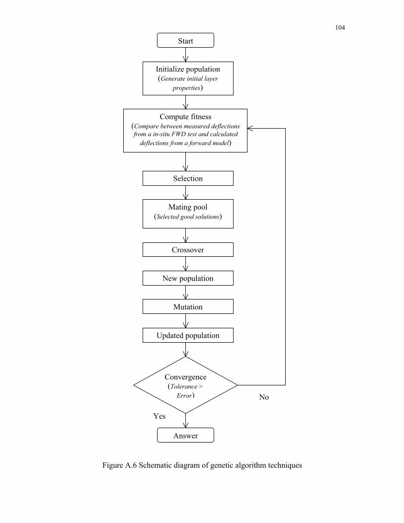
104
No
Yes
Answer
Convergence(Tolerance >
Error)
New population
Mutation
Crossover
Mating pool (Selected good solutions)
Selection
Compute fitness (Compare between measured deflections from a in-situ FWD test and calculated
deflections from a forward model)
Initialize population (Generate initial layer
properties)
Start
Updated population
Figure A.6 Schematic diagram of genetic algorithm techniques


