
Facility Design-Week13
Facility Location Problem
1
McDonald’s• QSCV Philosophy• 11,000 restaurants (7,000 in USA, remaining in 50
countries)• 700 seat McDonald’s in Pushkin Square, Moscow• $60 million food plant combining a bakery, lettuce plant,
meat plant, chicken plant, fish plant and a distribution center, each owned and operated independently at same location
2

McDonald’s cont...• Food taste must be the same at any McDonald, yet food
must be secured locally• Strong logistical chain, with no weak links between• Close monitoring for logistical performance• 300 in Australia• Central distribution since 1974 with the help of F.J. Walker
Foods in Sydney• Then distribution centers opened in several cities
3

McDonald’s cont...• 2000 ingredients, from 48 food plants, shipment of 200
finished products from suppliers to DC’s, 6 million cases of food and paper products plus 500 operating items to restaurants across Australia
• Delivery of frozen, dry and chilled foods twice a week to each of the 300 restaurants 98% of the time within 15 minutes of promised delivery time, 99.8% within 2 days of order placement
• No stockouts, but less inventory
4
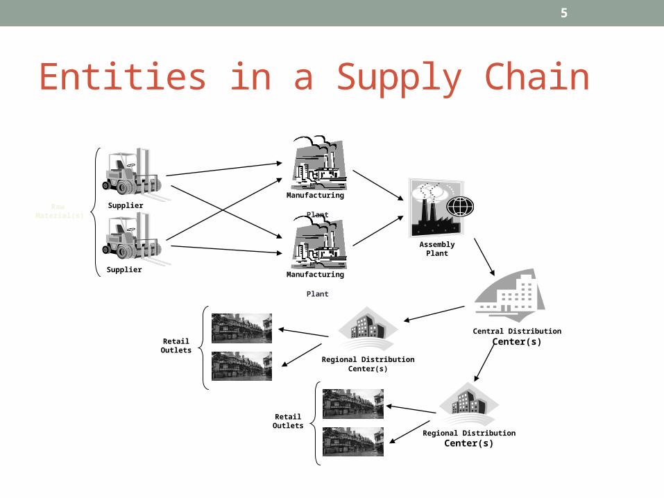
Entities in a Supply Chain
Supplier
Supplier
Manufacturing
Plant
Manufacturing
Plant
Raw Material(s)
Assembly Plant
Central Distribution Center(s)
Regional Distribution Center(s)
Regional Distribution Center(s)
Retail Outlets
Retail Outlets
5

Introduction• Design and Operation of a Supply chain
• Warehousing• Distribution Channels• Freight Transportation• Freight Consolidation• Transportation Modes
6

Introduction• Logistics management can be defined as the
management of transportation and distribution of goods.
• facility location• transportation• goods handling and storage.
7
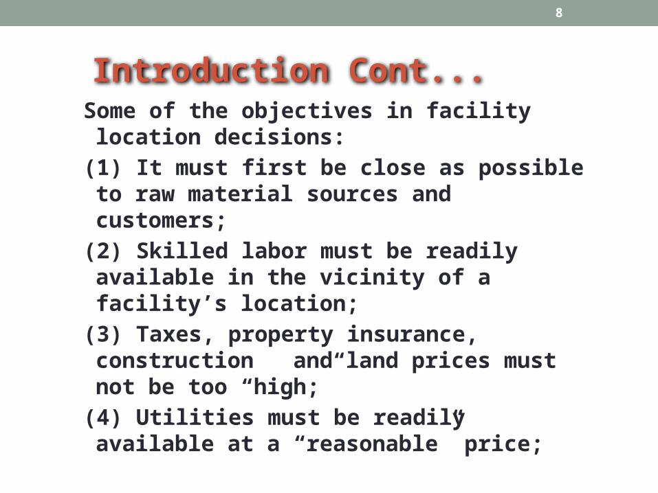
Introduction Cont...Some of the objectives in facility location
decisions:
(1) It must first be close as possible to raw material sources and customers;
(2) Skilled labor must be readily available in the vicinity of a facility’s location;
(3) Taxes, property insurance, construction and land prices must not be too “high;”
(4) Utilities must be readily available at a “reasonable” price;
8

Introduction Cont...(5) Local , state and other government regulations
must be conducive to business; and
(6) Business climate must be favorable and the community must have adequate support services and facilities such as schools, hospitals and libraries, which are important to employees and their families.
9
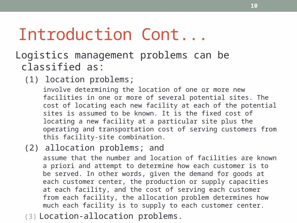
Introduction Cont...Logistics management problems can be classified as:
(1) location problems;involve determining the location of one or more new facilities in one or more of several potential sites. The cost of locating each new facility at each of the potential sites is assumed to be known. It is the fixed cost of locating a new facility at a particular site plus the operating and transportation cost of serving customers from this facility-site combination.
(2) allocation problems; and assume that the number and location of facilities are known a priori and attempt to determine how each customer is to be served. In other words, given the demand for goods at each customer center, the production or supply capacities at each facility, and the cost of serving each customer from each facility, the allocation problem determines how much each facility is to supply to each customer center.
(3) Location-allocation problems. involve determining not only how much each customer is to receive from each facility but also the number of facilities along with their locations and capacities.
10

List of Factors Affecting Location Decisions
• Proximity to raw materials sources• Cost and availability of energy/utilities• Cost, availability, skill and productivity of labor• Government regulations at the federal, state, country and
local levels• Taxes at the federal, state, county and local levels• Insurance• Construction costs, land price
11
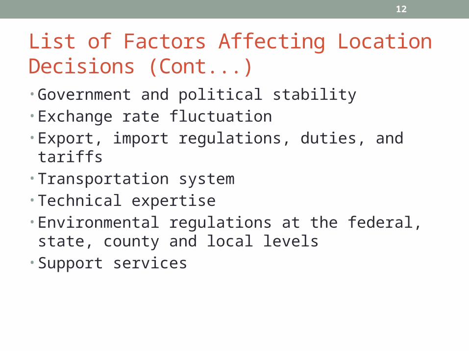
List of Factors Affecting Location Decisions (Cont...)• Government and political stability• Exchange rate fluctuation• Export, import regulations, duties, and tariffs• Transportation system• Technical expertise• Environmental regulations at the federal, state, county
and local levels• Support services
12

List of Factors Affecting Location Decisions (Cont...)• Community services, i.e. schools, hospitals, recreation,
etc.• Weather• Proximity to customers• Business climate• Competition-related factors
13

11.2Important Factors in Location Decisions
• International• National• State-wide• Community-wide
14

Qualitative AnalysisStep 1: List all the factors that are important, i.e. have an
impact on the location decision.
Step 2: Assign appropriate weights (typically between 0 and 1) to each factor based on the relative importance of each.
Step 3: Assign a score (typically between 0 and 100) for each location with respect to each factor identified in Step 1.
15

Qualitative AnalysisStep 4: Compute the weighted score for each factor for
each location by multiplying its weight with the corresponding score (which were assigned Steps 2 and 3, respectively)
Step 5: Compute the sum of the weighted scores for each location and choose a location based on these scores.
16

Example 1:•A payroll processing company has recently won several major contracts in the midwest region of the U.S. and central Canada and wants to open a new, large facility to serve these areas. Since customer service is of utmost importance, the company wants to be as near it’s “customers” as possible. Preliminary investigation has shown that Minneapolis, Winnipeg, and Springfield, Ill., would be the three most desirable locations and the payroll company has to select one of these three.
17
Example 1: Cont...
A subsequent thorough investigation of each location with respect to eight important factors has generated the raw scores and weights listed in table 2. Using the location scoring method, determine the best location for the new payroll processing facility.
18

Solution:
Steps 1, 2, and 3 have already been completed for us. We now need to compute the weighted score for each location-factor pair (Step 4), and these weighted scores and determine the location based on these scores (Step 5).
19

Table 1. Factors and Weights for Three Locations
Wt. Factors Location
Minn.Winn.Spring.
.25 Proximity to customers 95 9065
.15 Land/construction prices 60 6090
.15 Wage rates 70 45 60
.10 Property taxes 70 90 70
.10 Business taxes 80 90 85
.10 Commercial travel 80 65 75
20

Table 1.Cont...
Wt. Factors Location
Minn. Winn. Spring.
.08 Insurance costs 70 95 60
.07 Office services 90 90 80
21

Solution: Cont...
From the analysis in Table 2, it is clear that Minneapolis would be the best location based on the subjective information.
22
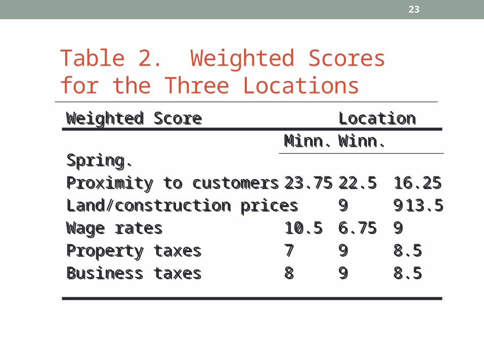
Table 2. Weighted Scores for the Three LocationsWeighted Score Location
Minn. Winn. Spring.
Proximity to customers 23.75 22.5 16.25
Land/construction prices 9 9 13.5
Wage rates 10.5 6.75 9
Property taxes 7 9 8.5
Business taxes 8 9 8.5
Weighted Score Location
Minn. Winn. Spring.
Proximity to customers 23.75 22.5 16.25
Land/construction prices 9 9 13.5
Wage rates 10.5 6.75 9
Property taxes 7 9 8.5
Business taxes 8 9 8.5
23

Table 2. Cont...
Weighted Score Location
Minn. Winn. Spring.
Commercial travel 8 6.5 7.5
Insurance costs 5.6 7.6 4.8
Office services 6.3 6.3 5.6
Weighted Score Location
Minn. Winn. Spring.
Commercial travel 8 6.5 7.5
Insurance costs 5.6 7.6 4.8
Office services 6.3 6.3 5.6
24

Solution: Cont...
Of course, as mentioned before, objective measures must be brought into consideration especially because the weighted scores for Minneapolis and Winnipeg are close.
25

QUANTITATIVE ANALYSIS
26

General Transportation Model
27

General Transportation Model
Parameters
cij: cost of transporting one unit from warehouse i to customer j
ai: supply capacity at warehouse i
bi: demand at customer j
Decision Variables
xij: number of units transported from warehouse i to customer j
28
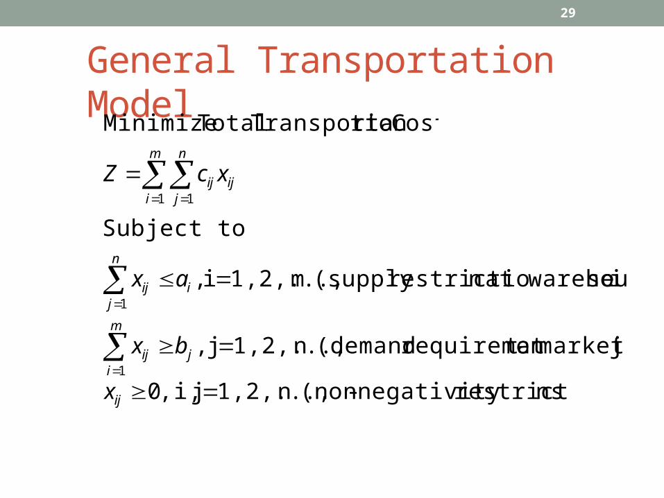
General Transportation Model
m
i
n
jijij xcZ
1 1
Costtion Transporta Total Minimize
i) seat warehoun restrictio(supply m1,2,...,i ,
Subject to
1
n
jiij ax
j)market at t requiremen (demandn 1,2,...,j ,1
m
ijij bx
ns)restrictio negativity-(nonn 1,2,...,ji, ,0 ijx
29
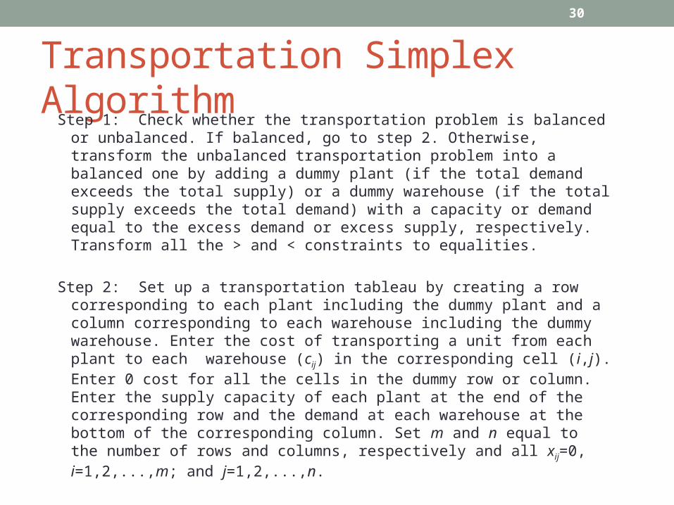
Transportation Simplex AlgorithmStep 1: Check whether the transportation problem is balanced or unbalanced.
If balanced, go to step 2. Otherwise, transform the unbalanced transportation problem into a balanced one by adding a dummy plant (if the total demand exceeds the total supply) or a dummy warehouse (if the total supply exceeds the total demand) with a capacity or demand equal to the excess demand or excess supply, respectively. Transform all the > and < constraints to equalities.
Step 2: Set up a transportation tableau by creating a row corresponding to each plant including the dummy plant and a column corresponding to each warehouse including the dummy warehouse. Enter the cost of transporting a unit from each plant to each warehouse (cij) in the corresponding cell (i,j). Enter 0 cost for all the cells in the dummy row or column. Enter the supply capacity of each plant at the end of the corresponding row and the demand at each warehouse at the bottom of the corresponding column. Set m and n equal to the number of rows and columns, respectively and all xij=0, i=1,2,...,m; and j=1,2,...,n.
Step 3: Construct a basic feasible solution using the Northwest corner method.
30

Transportation Simplex AlgorithmStep 4: Set u1=0 and find vj, j=1,2,...,n and ui, i=1,2,...,n using the formula ui
+ vj = cij for all basic variables.
Step 5: If ui + vj - cij < 0 for all nonbasic variables, then the current basic feasible solution is optimal; stop. Otherwise, go to step 6.
Step 6: Select the variable xi*j* with the most positive value ui* + vj*- cij*. Construct a closed loop consisting of horizontal and vertical segments connecting the corresponding cell in row i* and column j* to other basic variables. Adjust the values of the basic variables in this closed loop so that the supply and demand constraints of each row and column are satisfied and the maximum possible value is added to the cell in row i* and column j*. The variable xi*j* is now a basic variable and the basic variable in the closed loop which now takes on a value of 0 is a nonbasic variable. Go to step 4.
31

Example 2:Seers Inc. has two manufacturing plants at Albany and Little Rock supplying Canmore brand refrigerators to four distribution centers in Boston, Philadelphia, Galveston and Raleigh. Due to an increase in demand of this brand of refrigerators that is expected to last for several years into the future, Seers Inc., has decided to build another plant in Atlanta. The expected demand at the three distribution centers and the maximum capacity at the Albany and Little Rock plants are given in Table 4.
32

Table 3.Costs, Demand and Supply Information
Bost. Phil. Galv. Rale. Supply
Capacity
Albany 10 15 22 20 250
Little Rock 19 15 10 9 300
Atlanta 21 11 13 6 No limit
Demand 200 100 300 280
33
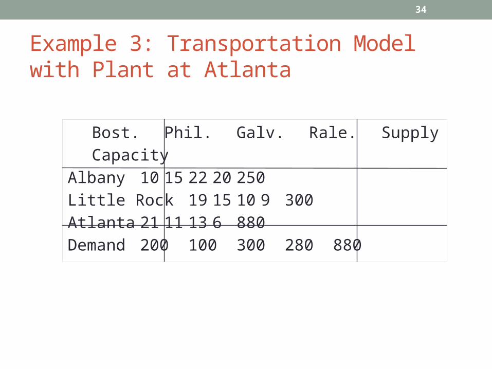
Example 3: Transportation Model with Plant at Atlanta
Bost. Phil. Galv. Rale. Supply
Capacity
Albany 10 15 22 20 250
Little Rock 19 15 10 9 300
Atlanta 21 11 13 6 880
Demand 200 100 300 280 880
34

Example 3
Consider Example 2. In addition to Atlanta, suppose Seers, Inc., is considering another location – Pittsburgh. Determine which of the two locations, Atlanta or Pittsburgh, is suitable for the new plant. Seers Inc., wishes to utilize all of the capacity available at it’s Albany and Little Rock Locations
35

Table 4. Costs, Demand and Supply Information
Bost. Phil. Galv. Rale. Supply
Capacity
Albany 10 15 22 20 250
Little Rock 19 15 10 9 300
Atlanta 21 11 13 6 330
Pittsburgh 17 8 18 12 330
Demand 200 100 300 280
36

Min/Max Location Problem:
Location
d11 d12
d21 d22
d1n
d2n
dm1 dm2 dmn
Site
37

Hybrid Analysis
• Critical• Objective• Subjective
38

Hybrid Analysis Cont...
CFij = 1 if location i satisfies critical factor j,
0 otherwise
OFij = cost of objective factor j at location i
SFij = numerical value assigned
(on scale of 0-100)
to subjective factor j for location i
wj = weight assigned to subjective factor
(0< w < 1)
39

Hybrid Analysis Cont...
OFMi
max i OFijj 1
q
OFij
j 1
q
max i OFijj 1
q
min i OFij
j 1
q
, i 1,2,...,m
SFMi w jSFijj 1
r
, i 1,2,...,m
mi
CFCFCFCFCFMp
jijipiii
,...,2,1
,1
21
40

Hybrid Analysis Cont...
The location measure LMi for each location is then calculated as:
LMi = CFMi [ OFMi + (1- ) SFMi ]
Where is the weight assigned to the objective factor.
We then choose the location with the highest location measure LMi
41

Example 4:Mole-Sun Brewing company is evaluating six candidate locations-Montreal, Plattsburgh, Ottawa, Albany, Rochester and Kingston, for constructing a new brewery. There are two critical, three objective and four subjective factors that management wishes to incorporate in its decision-making. These factors are summarized in Table 7. The weights of the subjective factors are also provided in the table. Determine the best location if the subjective factors are to be weighted 50 percent more than the objective factors.
42

CRITICAL, SUBJECTIVE AND OBJECTIVE FACTOR RATINGS FOR SIX LOCATIONS
FOR MOLE-SUN BREWING COMPANY, INC.
43

FactorsLocation
Albany 0 1
Kingston 1 1
Montreal 1 1
Ottawa 1 0
Plattsburgh 1 1
Rochester 1 1
Location
Albany 0 1
Kingston 1 1
Montreal 1 1
Ottawa 1 0
Plattsburgh 1 1
Rochester 1 1
CriticalCritical
Water
Supply
Water
SupplyTax
Incentives
Tax
Incentives
Table 5. Cont...
44
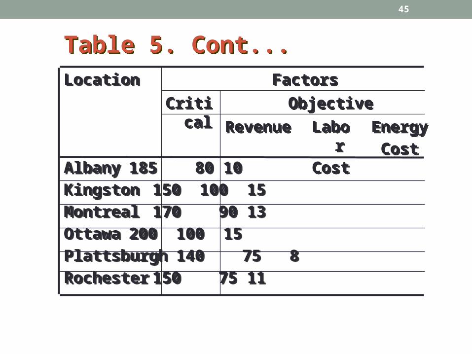
Table 5. Cont...Table 5. Cont...
FactorsFactorsLocation
Albany 185 80 10
Kingston 150 100 15
Montreal 170 90 13
Ottawa 200 100 15
Plattsburgh 140 75 8
Rochester 150 75 11
Location
Albany 185 80 10
Kingston 150 100 15
Montreal 170 90 13
Ottawa 200 100 15
Plattsburgh 140 75 8
Rochester 150 75 11
CriticalCritical
Labor
Cost
Labor
CostEnergy
Cost
Energy
Cost
ObjectiveObjective
RevenueRevenue
45

Location
0.3 0.4
Albany 0.5 0.9
Kingston 0.6 0.7
Montreal 0.4 0.8
Ottawa 0.5 0.4
Plattsburgh 0.9 0.9
Rochester 0.7 0.65
Location
0.3 0.4
Albany 0.5 0.9
Kingston 0.6 0.7
Montreal 0.4 0.8
Ottawa 0.5 0.4
Plattsburgh 0.9 0.9
Rochester 0.7 0.65
Table 4. Cont...Table 4. Cont...FactorsFactors
Ease of
Transportation
Ease of
Transportation
SubjectiveSubjective
Community
Attitude
Community
Attitude
46

Table 5. Cont...Table 5. Cont...FactorsFactorsLocation
0.25 0.05
Albany 0.6 0.7
Kingston 0.7 0.75
Montreal 0.2 0.8
Ottawa 0.4 0.8
Plattsburgh 0.9 0.55
Rochester 0.4 0.8
Location
0.25 0.05
Albany 0.6 0.7
Kingston 0.7 0.75
Montreal 0.2 0.8
Ottawa 0.4 0.8
Plattsburgh 0.9 0.55
Rochester 0.4 0.8
Support
Services
Support
Services
SubjectiveSubjective
Labor
Unionization
Labor
Unionization
47

LOCATION ANALYSIS OF MOLE-SUN BREWING COMPANY, INC.,
USING HYBRID METHOD
48

Location
Albany -95 0.7 0
Kingston -35 0.67 0.4
Montreal -67 0.53 0.53
Ottawa -85 0.45 0
Plattsburgh -57 0.88 0.68
Rochester -64 0.61 0.56
Location
Albany -95 0.7 0
Kingston -35 0.67 0.4
Montreal -67 0.53 0.53
Ottawa -85 0.45 0
Plattsburgh -57 0.88 0.68
Rochester -64 0.61 0.56
Table 5. Cont...Table 5. Cont...
FactorsFactors
SFMiSFMi
SubjectiveSubjective
Sum of
Obj. Factors
Sum of
Obj. Factors
CriticalCritical ObjectiveObjective LMi
49

TECHNIQUES FOR CONTINUOUS SPACE LOCATION
PROBLEMS
50

Model for Rectilinear Metric Problem
Consider the following notation:
fi = Traffic flow between new facility and existing facility i
ci = Cost of transportation between new facility and existing facility i per unit
xi, yi = Coordinate points of existing facility i
51

Model for Rectilinear Metric Problem (Cont)
Where TC is the total distribution cost
m
iiiii yyxxfc
1
]||||[ TC
The median location model is then to minimize:
52

Model for Rectilinear Metric Problem (Cont)
Since the cifi product is known for each facility, it can be thought of as a weight wi corresponding to facility i.
m
i
m
iiiii yywxxw
1 1
]||[]||[ TC Minimize
53

Median Method:
Step 1: List the existing facilities in non-decreasing order of the x coordinates.
Step 2: Find the jth x coordinate in the list at which the cumulative weight equals or exceeds half the total weight for the first time, i.e.,
j
i
m
i
ii
j
i
m
i
ii
ww
ww
1 1
1
1 1 2 and
2
54
Median Method (Cont)
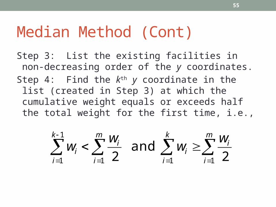
Step 3: List the existing facilities in non-decreasing order of the y coordinates.
Step 4: Find the kth y coordinate in the list (created in Step 3) at which the cumulative weight equals or exceeds half the total weight for the first time, i.e.,
k
i
m
i
ii
k
i
m
i
ii
ww
ww
1 1
1
1 1 2 and
2
55

Median Method (Cont)
Step 4: Cont... The optimal location of the new facility is given by the jth x coordinate and the kth y coordinate identified in Steps 2 and 4, respectively.
56

Notes
1. It can be shown that any other x or y coordinate will not be that of the optimal location’s coordinates
2. The algorithm determines the x and y coordinates of the facility’s optimal location separately
3. These coordinates could coincide with the x and y coordinates of two different existing facilities or possibly one existing facility
57

Example 5:
Two high speed copiers are to be located in the fifth floor of an office complex which houses four departments of the Social Security Administration. Coordinates of the centroid of each department as well as the average number of trips made per day between each department and the copiers’ yet-to-be-determined location are known and given in Table 9 below. Assume that travel originates and ends at the centroid of each department. Determine the optimal location, i.e., x, y coordinates, for the copiers.
58

CENTROID COORDINATES AND AVERAGE NUMBER OF TRIPS TO
COPIERS
59

Table 5. Centroid Coordinates and Average Number of Trips to Copiers
Dept. Coordinates Average number of
# x y daily trips to copiers
1 10 2 6
2 10 10 10
3 8 6 8
4 12 5 4
60
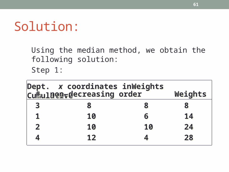
Solution:
Using the median method, we obtain the following solution:
Step 1:
Dept. x coordinates in Weights Cumulative Dept. x coordinates in Weights Cumulative # non-decreasing order Weights# non-decreasing order Weights
3 8 8 8
1 10 6 14
2 10 10 24
4 12 4 28
3 8 8 8
1 10 6 14
2 10 10 24
4 12 4 28
61

Solution:
Step 2: Since the second x coordinate, namely 10, in the above list is where the cumulative weight equals half the total weight of 28/2 = 14, the optimal x coordinate is 10.
62

Solution:
Step 3:
Dept. y coordinates in Weights Cumulative Dept. y coordinates in Weights Cumulative # non-decreasing order Weights# non-decreasing order Weights
1 2 6 6
4 5 4 10
3 6 8 18
2 10 10 28
1 2 6 6
4 5 4 10
3 6 8 18
2 10 10 28
63

Solution:
Step 4: Since the third y coordinates in the above list is where the cumulative weight exceeds half the total weight of 28/2 = 14, the optimal y coordinate is 6. Thus, the optimal coordinates of the new facility are (10, 6).
64

Equivalent Linear Model for the Rectilinear Distance, Single-Facility Location Problem
Parameters
fi = Traffic flow between new facility and existing facility i
ci = Unit transportation cost between new facility and existing facility i
xi, yi = Coordinate points of existing facility iDecision Variables x, y = Optimal coordinates of the new facility TC = Total distribution cost
65

Equivalent Linear Model for the Rectilinear Distance, Single-Facility Location Problem
The median location model is then to
m
i
m
iiiii yywxxw
1 1
]||[]||[ TC Minimize
66

Equivalent Linear Model for the Rectilinear Distance, Single-Facility Location Problem
Since the cifi product is known for each facility, it can be
thought of as a weight wi corresponding to facility i. The
previous equation can now be rewritten as follows
m
i
m
iiiii yywxxw
1 1
]||[]||[ TC Minimize
67

Equivalent Linear Model for the Rectilinear Distance, Single-Facility Location Problem
iii
iii
i
iii
iii
xxxx
xxxx
xx
xxxxx
xxxxx
)(
and
0, or 0)( whether that,observecan We
otherwise 0
0 if )(
otherwise 0
0 if )(
Define
68
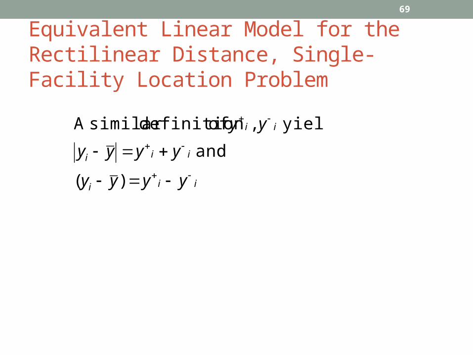
Equivalent Linear Model for the Rectilinear Distance, Single-Facility Location Problem
iii
iii
ii
yyyy
yyyy
yy
)(
and
yields , of definitionsimilar A
69

n
i
iiiii yyxxw1
)( Minimize
ModelLinear dTransforme
signin edunrestrict ,,
n1,2,...,i 0, ,,,
n1,2,...,i ,-)(
n1,2,...,i ,-)(
Subject to
yx
yyxx
yyyy
xxxx
iiii
iii
iii
Equivalent Linear Model for the Rectilinear Distance, Single-Facility Location Problem
70

CONTOUR LINE METHOD
71

Algorithm for Drawing Contour Lines:
Step 1: Draw a vertical line through the x coordinate and a horizontal line through the y coordinate of each facility
Step 2: Label each vertical line Vi, i=1, 2, ..., p and horizontal line Hj, j=1, 2, ..., q where Vi= the sum of weights of facilities whose x coordinates fall on vertical line i and where Hj= sum of weights of facilities whose y coordinates fall on horizontal line j
72
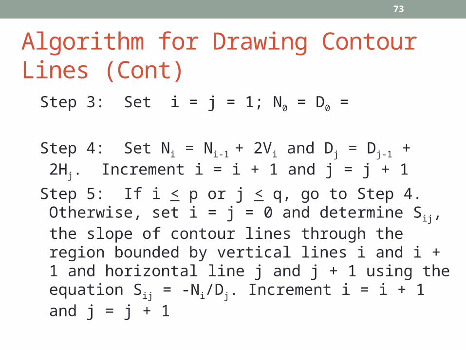
Algorithm for Drawing Contour Lines (Cont)
Step 3: Set i = j = 1; N0 = D0 =
Step 4: Set Ni = Ni-1 + 2Vi and Dj = Dj-1 + 2Hj. Increment i = i + 1 and j = j + 1
Step 5: If i < p or j < q, go to Step 4. Otherwise, set i = j = 0 and determine Sij, the slope of contour lines through the region bounded by vertical lines i and i + 1 and horizontal line j and j + 1 using the equation Sij = -Ni/Dj. Increment i = i + 1 and j = j + 1
73

Algorithm for Drawing Contour Lines:
Step 6: If i < p or j < q, go to Step 5. Otherwise select any point (x, y) and draw a contour line with slope Sij in the region [i, j] in which (x, y) appears so that the line touches the boundary of this line. From one of the end points of this line, draw another contour line through the adjacent region with the corresponding slope
Step 7: Repeat this until you get a contour line ending at point (x, y). We now have a region bounded by contour lines with (x, y) on the boundary of the region
74
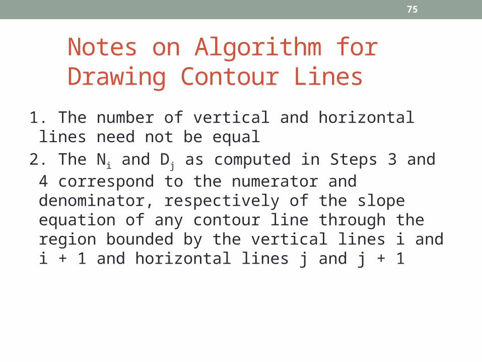
Notes on Algorithm for Drawing Contour Lines
1. The number of vertical and horizontal lines need not be equal
2. The Ni and Dj as computed in Steps 3 and 4 correspond to the numerator and denominator, respectively of the slope equation of any contour line through the region bounded by the vertical lines i and i + 1 and horizontal lines j and j + 1
75

Notes on Algorithm for Drawing Contour Lines (Cont)
yywxxwTC
yyxx
i
m
iii
m
ii
11
, i.e., y),(x,point someat located is
facility new hen thefunction w objective heConsider t
76

Notes on Algorithm for Drawing Contour Lines (Cont)
By noting that the Vi’s and Hj’s calculated in Step 2 of the algorithm correspond to the sum of the weights of facilities whose x, y coordinates are equal to the x, y coordinates, respectively of the ith, jth distinct lines and that we have p, q such coordinates or lines (p < m, q < m), the previous equation can be written as follows
yyHxxVTC i
q
iii
p
ii
11
77

Notes on Algorithm for Drawing Contour Lines (Cont)
Suppose that x is between the sth and s+1th (distinct) x coordinates or vertical lines (since we have drawn vertical lines through these coordinates in Step 1). Similarly, let y be between the tth and t+1th vertical lines. Then
TC Vi(i1
s
x x i) Viis1
p
(x i x)
Hi(i1
t
y y i) Hiit1
q
(y i y)
78

Notes on Algorithm for Drawing Contour Lines (Cont)Rearranging the variable and constant terms in the above equation, we get
i
q
tiii
t
iii
p
siii
s
ii
t
i
q
tiii
s
i
p
siii
yHyHxVxV
yHHxVVTC
1111
1 11 1
79
Notes on Algorithm for Drawing Contour Lines (Cont)
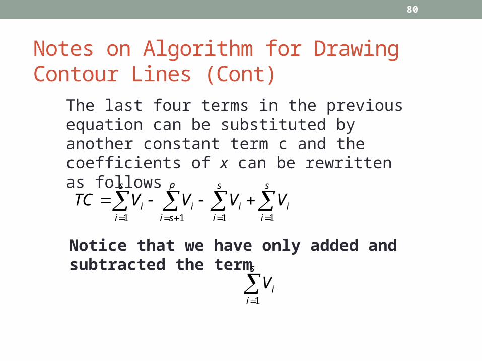
The last four terms in the previous equation can be substituted by another constant term c and the coefficients of x can be rewritten as follows
s
i
s
iii
s
i
p
siii VVVVTC
1 11 1
Notice that we have only added and subtracted the term
s
iiV
1
80

Since it is clear from Step 2 thatSince it is clear from Step 2 that
the coefficient of x can be rewritten asthe coefficient of x can be rewritten as
Notes on Algorithm for Drawing Contour Lines (Cont)
,11
m
ii
s
ii wV
s
i
m
iii
s
i
p
iii
s
i
p
sii
s
iii
wV
VVVVV
1 1
1 11 11
2
22
Similarly, the coefficient of y isSimilarly, the coefficient of y is
t
i
m
iii wH
1 1
2
81

cywHxwVt
i
m
iii
s
i
m
iii
1 11 1
22TC Thus,
Notes on Algorithm for Drawing Contour Lines (Cont)
• The Ni computation in Step 4 is in fact calculation of the coefficient of x as shown above. Note that Ni=Ni-1+2Vi. Making the substitution for Ni-1, we get Ni=Ni-2+2Vi-1+2Vi
• Repeating the same procedure of making substitutions for Ni-2, Ni-3, ..., we get
• Ni=N0+2V1+2V2+...+2Vi-1+2V1=
i
kk
m
ii Vw
11
2
82

Notes on Algorithm for Drawing Contour Lines (Cont)
Similarly, it can be verified that
i
kk
m
iii HwD
11
2
)(
asrewritten becan which
22TC Thus,1 11 1
cTCxD
Ny
cyDxN
cywHxwV
t
s
ts
t
i
m
iii
s
i
m
iii
83
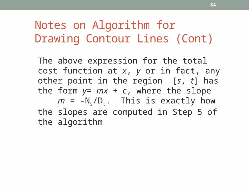
Notes on Algorithm for Drawing Contour Lines (Cont)The above expression for the total cost function at x, y or in fact, any other point in the region [s, t] has the form y= mx + c, where the slope m = -Ns/Dt. This is exactly how the slopes are computed in Step 5 of the algorithm
84

Notes on Algorithm for Drawing Contour Lines (Cont)
3. The lines V0, Vp+1 and H0, Hq+1 are required for defining the “exterior” regions [0, j], [p, j], j = 1, 2, ..., p, respectively)
4. Once we have determined the slopes of all regions, the user may choose any point (x, y) other than a point which minimizes the objective function and draw a series of contour lines in order to get a region which contains points, i.e. facility locations, yielding as good or better objective function values than (x, y)
85

Example 6:
Consider Example 5. Suppose that the weight of facility 2 is not 10, but 20. Applying the median method, it can be verified that the optimal location is (10, 10) - the centroid of department 2, where immovable structures exist. It is now desired to find a feasible and “near-optimal” location using the contour line method.
86

Solution:The contour line method is illustrated using the figure below
87

Solution:
Step 1: The vertical and horizontal lines V1, V2, V2 and H1, H2, H2, H4 are drawn as shown. In addition to these lines, we also draw line V0, V4 and H0, H5 so that the “exterior regions can be identified
Step 2: The weights V1, V2, V2, H1, H2, H2, H4 are calculated by adding the weights of the points that fall on the respective lines. Note that for this example, p=3, and q=4
88

Solution:
Step 3: SinceStep 3: Since
set N0 = D0 = -38
Step 4: SetN1 = -38 + 2(8) = -22; D1 = -38 + 2(6) = -
26;N2 = -22 + 2(26) = 30; D2 = -26 + 2(4) = -18;N3 = 30 + 2(4) = 38; D3 = -18 + 2(8) = -2;
D4 = -2 + 2(20) = 38;
(These values are entered at the bottom of each column and left of each row in figure 1)
set N0 = D0 = -38
Step 4: SetN1 = -38 + 2(8) = -22; D1 = -38 + 2(6) = -
26;N2 = -22 + 2(26) = 30; D2 = -26 + 2(4) = -18;N3 = 30 + 2(4) = 38; D3 = -18 + 2(8) = -2;
D4 = -2 + 2(20) = 38;
(These values are entered at the bottom of each column and left of each row in figure 1)
384
1
i
iw
89
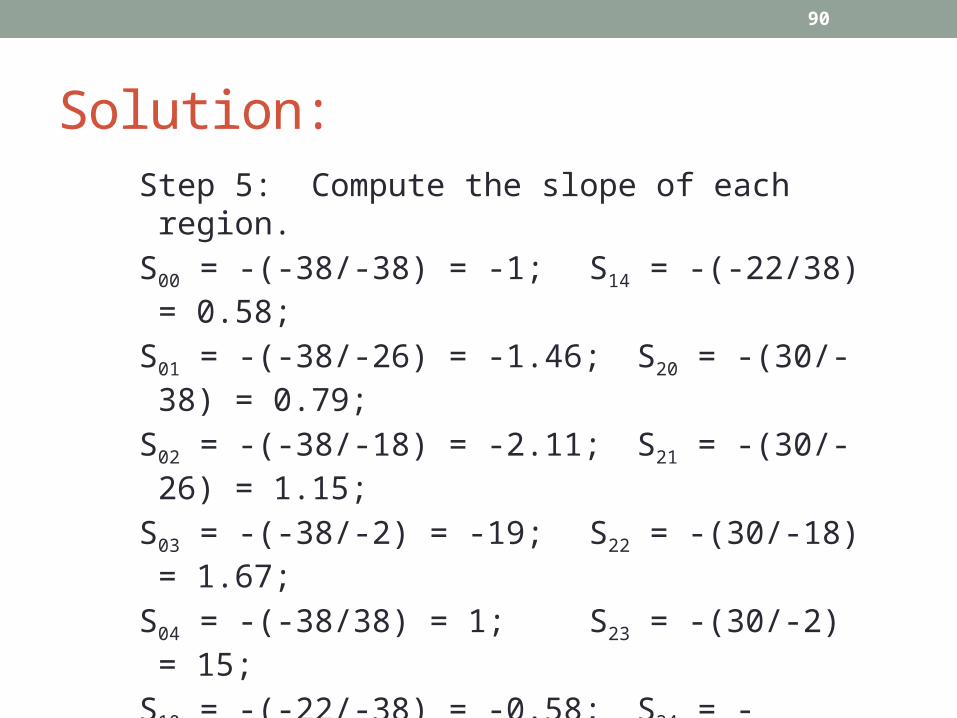
Solution:Step 5: Compute the slope of each region.
S00 = -(-38/-38) = -1; S14 = -(-22/38) = 0.58;
S01 = -(-38/-26) = -1.46; S20 = -(30/-38) = 0.79;
S02 = -(-38/-18) = -2.11; S21 = -(30/-26) = 1.15;
S03 = -(-38/-2) = -19; S22 = -(30/-18) = 1.67;
S04 = -(-38/38) = 1; S23 = -(30/-2) = 15;
S10 = -(-22/-38) = -0.58; S24 = -(30/38) = -0.79;
S11 = -(-22/-26) = -0.85; S30 = -(38/-38) = 1;
S12 = -(-22/-18) = -1.22; S31 = -(38/-26) = 1.46;
S13 = -(-22/-2) = -11; S32 = -(38/-18) = 2.11;
90
Solution:
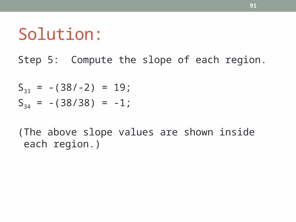
Step 5: Compute the slope of each region.
S33 = -(38/-2) = 19;
S34 = -(38/38) = -1;
(The above slope values are shown inside each region.)
91
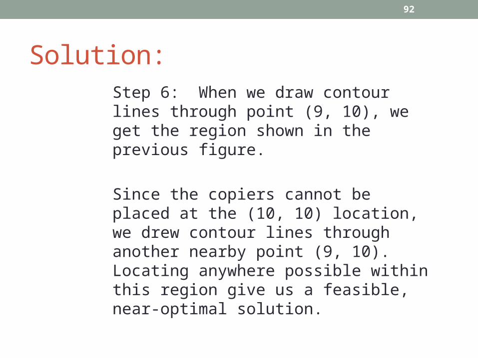
Solution:Step 6: When we draw contour lines through point (9, 10), we get the region shown in the previous figure.
Since the copiers cannot be placed at the (10, 10) location, we drew contour lines through another nearby point (9, 10). Locating anywhere possible within this region give us a feasible, near-optimal solution.
92

11.4.3SINGLE-FACILITY
LOCATION PROBLEM WITH SQUARED
EUCLIDEAN DISTANCES
93

La Quinta Motor Inns
Moderately priced, oriented towards business travelers
Headquartered in San Antonio Texas
Site selection - an important decision
Regression Model based on location characteristics classified as:
• Competitive, Demand Generators, Demographic, Market Awareness, and Physical
94

La Quinta Motor Inns (Cont)
Major Profitability Factors - Market awareness, hotel space, local population, low unemployment, accessibility to downtown office space, traffic count, college students, presence of military base, median income, competitive rates
95

Gravity Method:
As before, we substitute wi = fi ci, i = 1, 2, ..., m and rewrite the objective function as
Minimize TC c i f i (x i x )2 (yi y )2 i1
m
2
11
2 )()( TC Minimize yywxxw i
m
ii
m
iii
The cost function is
96

Gravity Method (Cont)
Since the objective function can be shown to be convex, partially differentiating TC with respect to x and y, setting the resulting two equations to 0 and solving for x, y provides the optimal location of the new facility
m
1i
m
1i
m
1i
m
1i
022 x
TC
iii
iii
wxwx
xwxw
97

Gravity Method (Cont)Similarly,
m
1i
m
1i
m
1i
m
1i
022 y
TC
iii
iii
wywy
ywyw
Thus, the optimal locations x and y are simply the weighted averages of the x and y coordinates of the existing facilities
98

Example 7:
Consider Example 5. Suppose the distance metric to be used is squared Euclidean. Determine the optimal location of the new facility using the gravity method.
99

Solution - Table 11.16
Department i xi yi wi wixi wiyiDepartment i xi yi wi wixi wiyi
1 10 2 6 60 12
2 10 10 10 100 100
3 8 6 8 64 48
4 12 5 4 48 20
1 10 2 6 60 12
2 10 10 10 100 100
3 8 6 8 64 48
4 12 5 4 48 20
Total 28 272 180Total 28 272 180
4.628180 and 7.928272
thatconclude we10, tableFrom
yx
100
Example 6. Cont...
If this location is not feasible, we only need to find another point which has the nearest Euclidean distance to (9.7, 6.4) and is a feasible location for the new facility and locate the copiers there
101

WEISZFELDMETHOD
102
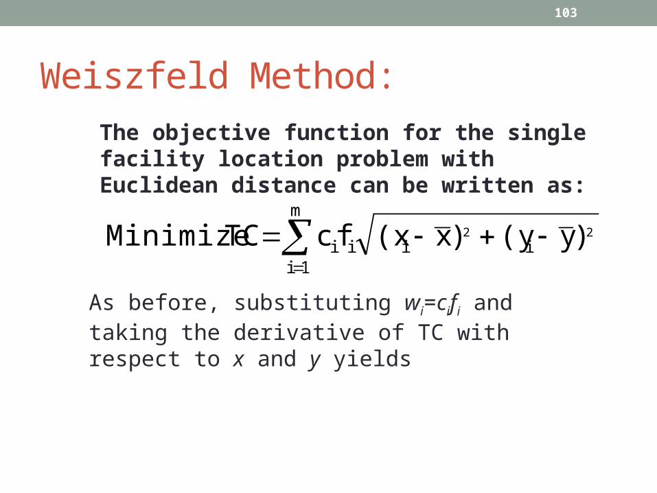
Weiszfeld Method:
As before, substituting wi=cifi and taking the derivative of TC with respect to x and y yields
)y(y)x(xfc TC Minimizem
1iiiii
22
The objective function for the single facility location problem with Euclidean distance can be written as:
103

Weiszfeld Method:
m
1i ii
i
m
1i ii
ii
m
1i ii
ii
0)y(y)x(x
xw
)y(y)x(x
xw
)y(y)x(x
)x2(xw
2
1
x
TC
22
22
22
104

Weiszfeld Method:
)y(y)x(x
w
)y(y)x(x
xw
x m
1i ii
i
m
1i ii
ii
22
22
105

Weiszfeld Method:
m
1i ii
i
m
1i ii
ii
m
1i ii
ii
0)y(y)x(x
yw
)y(y)x(x
yw
)y(y)x(x
)y2(yw
2
1
y
TC
22
22
22
106
Weiszfeld Method:
m
1i ii
i
m
1i ii
ii
22
22
)y(y)x(x
w
)y(y)x(x
yw
y
107

Weiszfeld Method:Step 0: Set iteration counter k = 1; Step 0: Set iteration counter k = 1;
m
m
m
m
1ii
1iii
k
1ii
1iii
k
w
ywy ;
w
xwx
108

Weiszfeld Method:Step 1: Set
Step 2: If xk+1 = xk and yk+1 = yk, Stop. Otherwise, set k = k + 1 and go to Step 1
Step 1: Set
Step 2: If xk+1 = xk and yk+1 = yk, Stop. Otherwise, set k = k + 1 and go to Step 1
m
iii
i
m
iii
ii
k
yyxx
w
yyxx
xw
x
122
122
1
m
iii
i
m
iii
ii
k
yyxx
w
yyxx
yw
y
122
122
1
109

Example 8:
Consider Example 6. Assuming the distance metric to be used is Euclidean, determine the optimal location of the new facility using the Weiszfeld method. Data for this problem is shown in Table 11.
110

Table 7:Coordinates and weights for4 departments
Departments # xi yi wiDepartments # xi yi wi
1 10 2 6
2 10 10 20
3 8 6 8
4 12 5 4
1 10 2 6
2 10 10 20
3 8 6 8
4 12 5 4
111

Summary: Methods for Single-Facility, Continuous Space Location Problems
• Problem• Rectilinear• Squared Euclidean• Euclidean
• Method• Median• Gravity• Weiszfeld


