Download - Experiments and Quasi-Experiments - uio.no
SW Ch. 13 1/67
Experiments and Quasi-Experiments (SW Chapter 13)
Outline
1. Potential Outcomes, Causal Effects, and Idealized
Experiments
2. Threats to Validity of Experiments
3. Application: The Tennessee STAR Experiment
4. Quasi-Experiments: Differences-in-Differences, IV
Estimation, Regression Discontinuity Design, and
Other Approaches.
5. Threats to Validity of Quasi-Experiments
6. Heterogeneous Causal Effects
SW Ch. 13 2/67
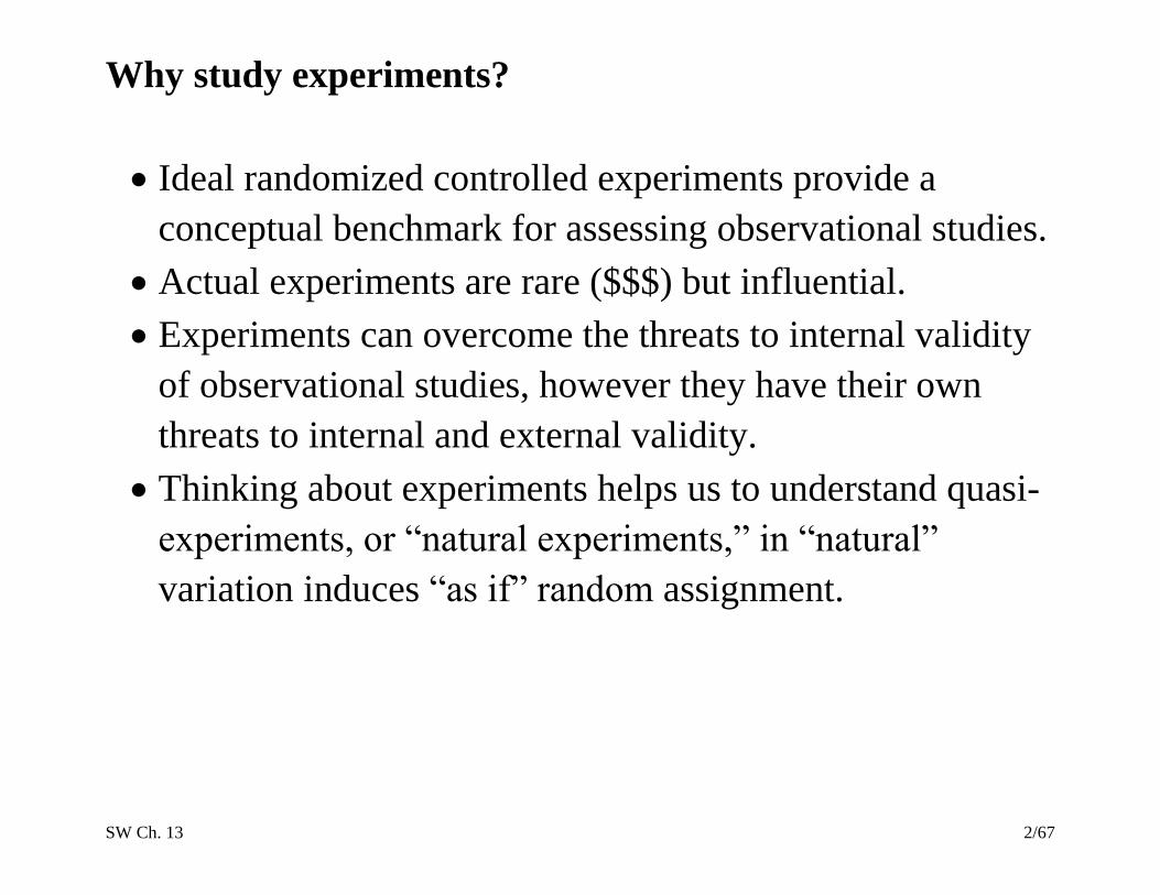
Why study experiments?
Ideal randomized controlled experiments provide a
conceptual benchmark for assessing observational studies.
Actual experiments are rare ($$$) but influential.
Experiments can overcome the threats to internal validity
of observational studies, however they have their own
threats to internal and external validity.
Thinking about experiments helps us to understand quasi-
experiments, or “natural experiments,” in “natural”
variation induces “as if” random assignment.
SW Ch. 13 3/67
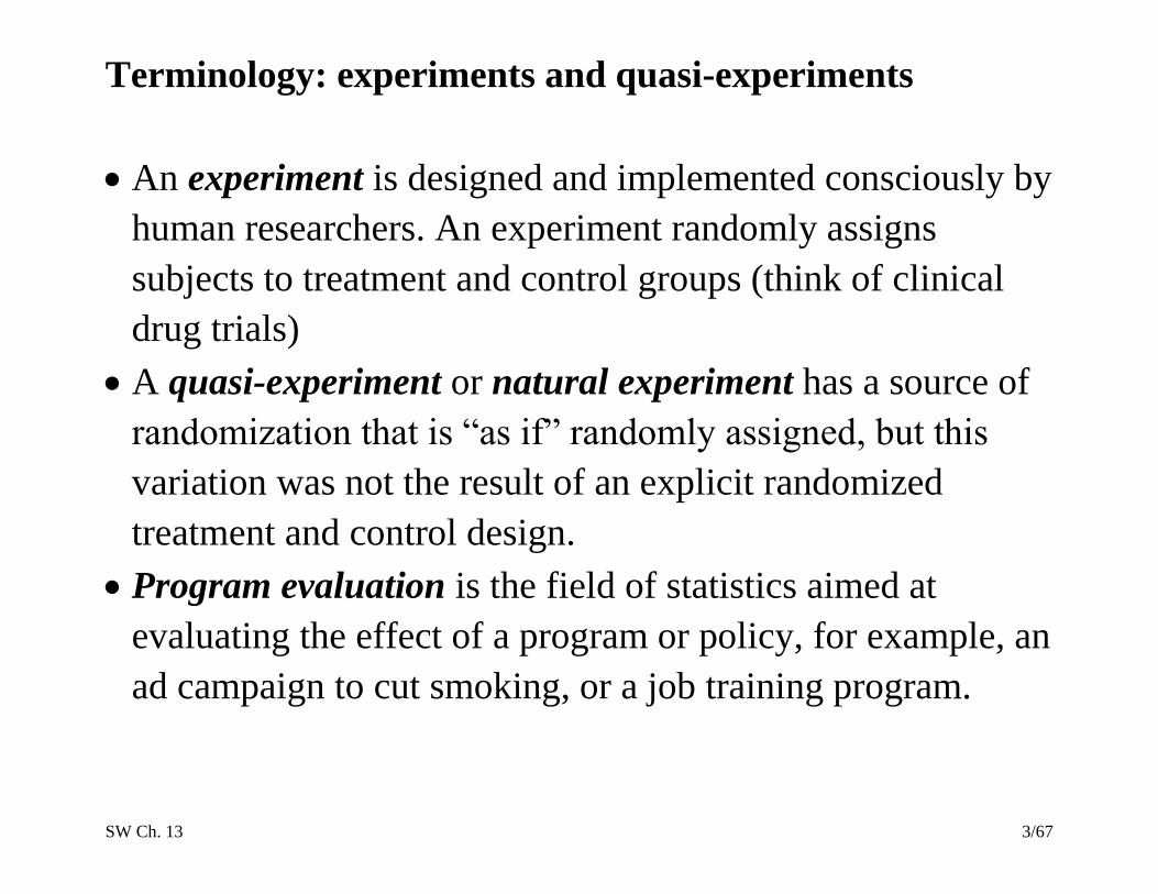
Terminology: experiments and quasi-experiments
An experiment is designed and implemented consciously by
human researchers. An experiment randomly assigns
subjects to treatment and control groups (think of clinical
drug trials)
A quasi-experiment or natural experiment has a source of
randomization that is “as if” randomly assigned, but this
variation was not the result of an explicit randomized
treatment and control design.
Program evaluation is the field of statistics aimed at
evaluating the effect of a program or policy, for example, an
ad campaign to cut smoking, or a job training program.
SW Ch. 13 4/67
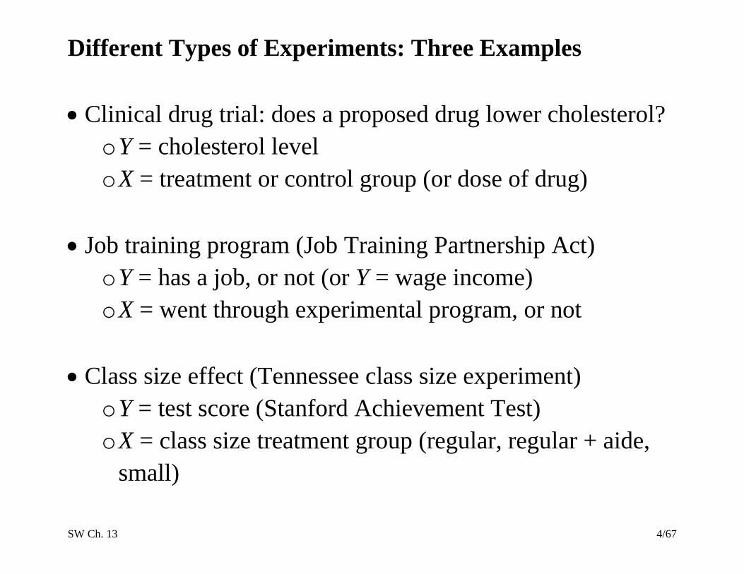
Different Types of Experiments: Three Examples
Clinical drug trial: does a proposed drug lower cholesterol?
o Y = cholesterol level
o X = treatment or control group (or dose of drug)
Job training program (Job Training Partnership Act)
o Y = has a job, or not (or Y = wage income)
o X = went through experimental program, or not
Class size effect (Tennessee class size experiment)
o Y = test score (Stanford Achievement Test)
o X = class size treatment group (regular, regular + aide,
small)
SW Ch. 13 5/67
Potential Outcomes, Causal Effects, and Idealized
Experiments
(SW Section 13.1)
A treatment has a causal effect for a given individual: give the
individual the treatment and something happens, which is
(possibly) different than what happens if you don’t get the
treatment.
A potential outcome is the outcome for an individual
under a potential treatment or potential non-treatment.
For an individual, the causal effect is the difference in
potential outcomes if you do or don’t get the treatment.
An individual’s causal effect cannot be observed because
you can give the subject the treatment, or not – but not
both!
SW Ch. 13 6/67
Average Treatment Effect
In general, different people have different treatment
effects. For people drawn from a population, the average
treatment effect is the population mean value of the
individual treatment effects.
For now, consider the case of a single treatment effect –
that everyone’s treatment effect is the same in the
population under study.
SW Ch. 13 7/67
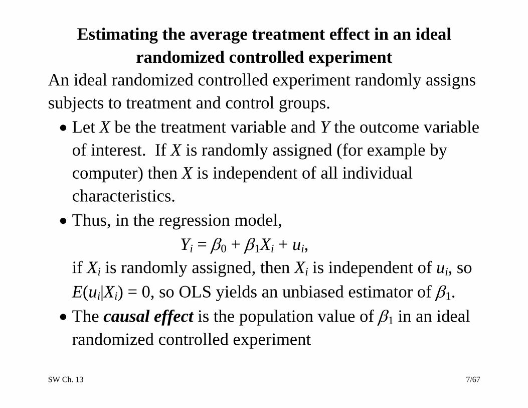
Estimating the average treatment effect in an ideal
randomized controlled experiment
An ideal randomized controlled experiment randomly assigns
subjects to treatment and control groups.
Let X be the treatment variable and Y the outcome variable
of interest. If X is randomly assigned (for example by
computer) then X is independent of all individual
characteristics.
Thus, in the regression model,
Yi = 0 + 1Xi + ui,
if Xi is randomly assigned, then Xi is independent of ui, so
E(ui|Xi) = 0, so OLS yields an unbiased estimator of 1.
The causal effect is the population value of 1 in an ideal
randomized controlled experiment
SW Ch. 13 8/67
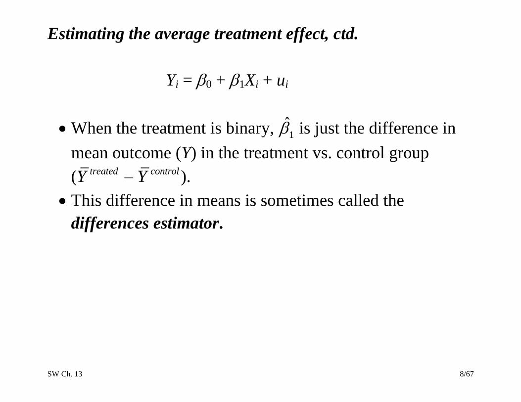
Estimating the average treatment effect, ctd.
Yi = 0 + 1Xi + ui
When the treatment is binary, 1̂ is just the difference in
mean outcome (Y) in the treatment vs. control group
( treatedY – controlY ).
This difference in means is sometimes called the
differences estimator.
SW Ch. 13 9/67
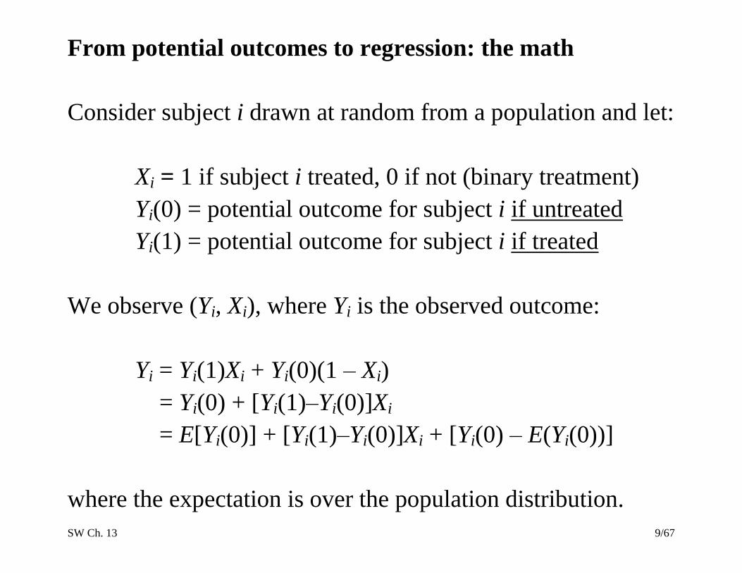
From potential outcomes to regression: the math
Consider subject i drawn at random from a population and let:
Xi = 1 if subject i treated, 0 if not (binary treatment)
Yi(0) = potential outcome for subject i if untreated
Yi(1) = potential outcome for subject i if treated
We observe (Yi, Xi), where Yi is the observed outcome:
Yi = Yi(1)Xi + Yi(0)(1 – Xi)
= Yi(0) + [Yi(1)–Yi(0)]Xi
= E[Yi(0)] + [Yi(1)–Yi(0)]Xi + [Yi(0) – E(Yi(0))]
where the expectation is over the population distribution.

SW Ch. 13 10/67
Potential outcomes to regression, ctd.
Thus
Yi = E[Yi(0)] + [Yi(1)–Yi(0)]Xi + [Yi(0) – E(Yi(0))]
= 0i + 1i Xi + ui
where
0 = E[Yi(0)]
1i = Yi(1)–Yi(0) = individual causal effect
ui = Yi(0) – E(Yi(0)), so Eui = 0.
When there is a single treatment effect – the case we consider
here – then 1i = 1 so we obtain the usual regression model,
Yi = 0 + 1Xi + ui
where 1 is the treatment (causal) effect.
SW Ch. 13 11/67
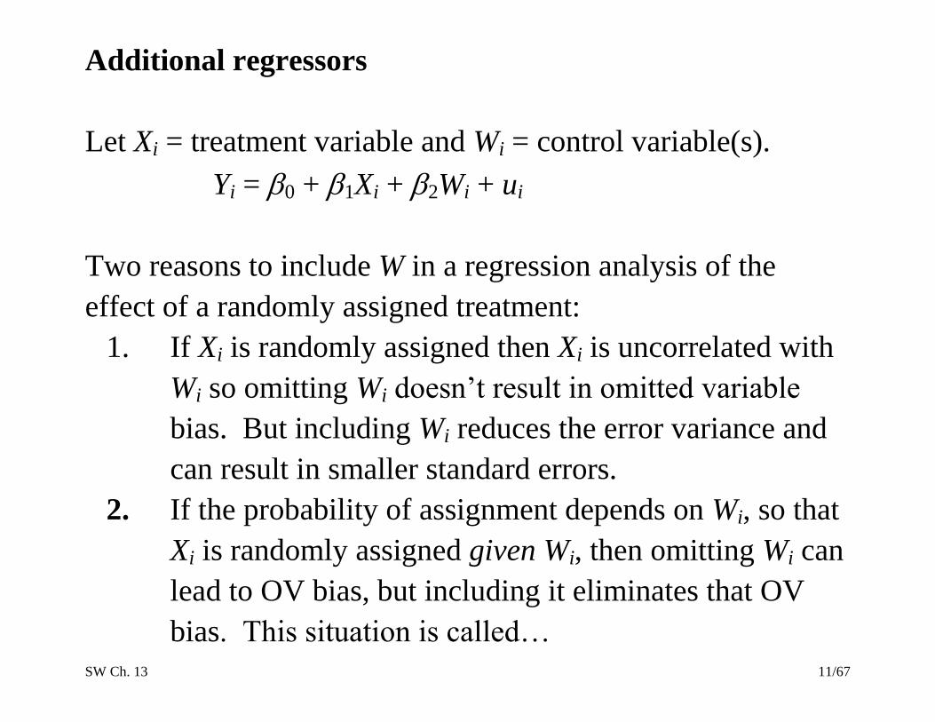
Additional regressors
Let Xi = treatment variable and Wi = control variable(s).
Yi = 0 + 1Xi + 2Wi + ui
Two reasons to include W in a regression analysis of the
effect of a randomly assigned treatment:
1. If Xi is randomly assigned then Xi is uncorrelated with
Wi so omitting Wi doesn’t result in omitted variable
bias. But including Wi reduces the error variance and
can result in smaller standard errors.
2. If the probability of assignment depends on Wi, so that
Xi is randomly assigned given Wi, then omitting Wi can
lead to OV bias, but including it eliminates that OV
bias. This situation is called…
SW Ch. 13 12/67
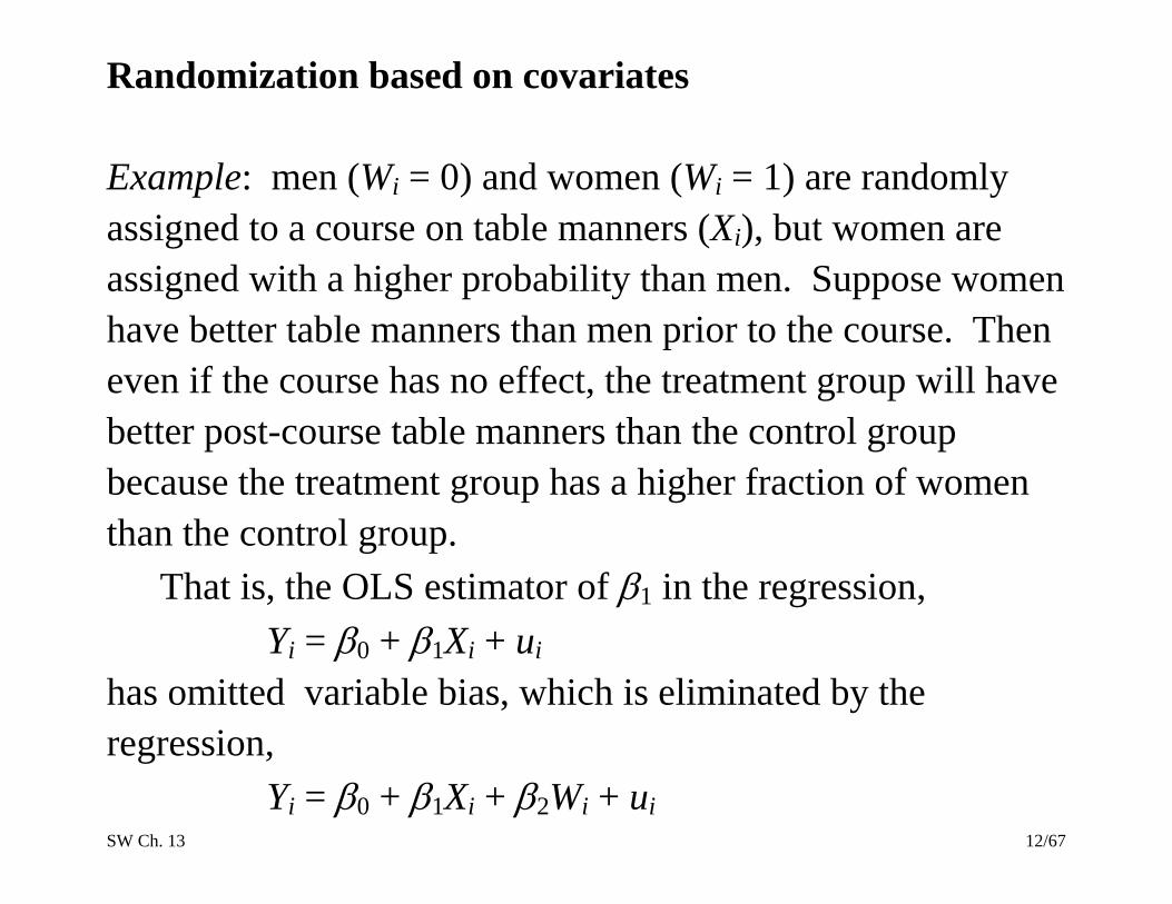
Randomization based on covariates
Example: men (Wi = 0) and women (Wi = 1) are randomly
assigned to a course on table manners (Xi), but women are
assigned with a higher probability than men. Suppose women
have better table manners than men prior to the course. Then
even if the course has no effect, the treatment group will have
better post-course table manners than the control group
because the treatment group has a higher fraction of women
than the control group.
That is, the OLS estimator of 1 in the regression,
Yi = 0 + 1Xi + ui
has omitted variable bias, which is eliminated by the
regression,
Yi = 0 + 1Xi + 2Wi + ui

SW Ch. 13 13/67
Randomization based on covariates, ctd.
Yi = 0 + 1Xi + 2Wi + ui
In this example, Xi is randomly assigned, given Wi, so
E(ui|Xi, Wi) = E(ui|Wi).
o In words, among women, treatment is randomly
assigned, so among women, the error term is
independent of Xi so, among women, its mean doesn’t
depend on Xi. Same is true among men.
Thus if randomization is based on covariates, conditional
mean independence holds, so that once Wi is included in
the regression the OLS estimator is unbiased as was
discussed in Ch. 7.
SW Ch. 13 14/67
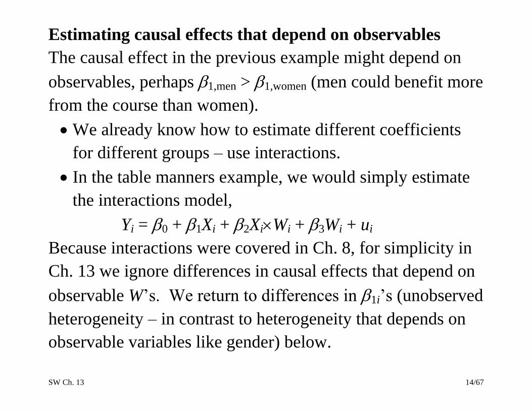
Estimating causal effects that depend on observables
The causal effect in the previous example might depend on
observables, perhaps 1,men > 1,women (men could benefit more
from the course than women).
We already know how to estimate different coefficients
for different groups – use interactions.
In the table manners example, we would simply estimate
the interactions model,
Yi = 0 + 1Xi + 2XiWi + 3Wi + ui
Because interactions were covered in Ch. 8, for simplicity in
Ch. 13 we ignore differences in causal effects that depend on
observable W’s. We return to differences in 1i’s (unobserved
heterogeneity – in contrast to heterogeneity that depends on
observable variables like gender) below.
SW Ch. 13 15/67
Threats to Validity of Experiments
(SW Section 13.2)
Threats to Internal Validity
1. Failure to randomize (or imperfect randomization)
for example, openings in job treatment program are
filled on first-come, first-serve basis; latecomers are
controls
result is correlation between X and u
SW Ch. 13 16/67
Threats to internal validity, ctd.
2. Failure to follow treatment protocol (or “partial
compliance”)
some controls get the treatment
some of those who should be treated aren’t
If you observe whether the subject actually receives
treatment (X), if you know whether the individual was
initially assigned to a treatment group (Z), and if initial
assignment was random, then you can estimate the
causal effect using initial assignment as an instrument
for actual treatment.
SW Ch. 13 17/67
Threats to internal validity, ctd.
3. Attrition (some subjects drop out)
Suppose the controls who get jobs move out of town;
then corr(X,u) 0
This is a reincarnation of sample selection bias from Ch.
9 (the sample is selected in a way related to the outcome
variable).
SW Ch. 13 18/67
Threats to internal validity, ctd.
4. Experimental effects
experimenter bias (conscious or subconscious):
treatment X is associated with “extra effort” or “extra
care,” so corr(X,u) 0
subject behavior might be affected by being in an
experiment, so corr(X,u) 0 (Hawthorne effect)
Just as in regression analysis with observational data,
threats to the internal validity of regression with
experimental data implies that corr(X,u) 0 so OLS (the
differences estimator) is biased.

SW Ch. 13 19/67
Threats to External Validity
1. Nonrepresentative sample
2. Nonrepresentative “treatment” (that is, program or policy)
3. General equilibrium effects (effect of a program can
depend on its scale; admissions counseling )

SW Ch. 13 20/67
Experimental Estimates of the Effect of
Class Size Reductions
(SW Section 13.3)
Project STAR (Student-Teacher Achievement Ratio)
4-year study, $12 million
Upon entering the school system, a student was randomly
assigned to one of three groups:
o regular class (22 – 25 students)
o regular class + aide
o small class (13 – 17 students)
regular class students re-randomized after first year to
regular or regular+aide
Y = Stanford Achievement Test scores
SW Ch. 13 21/67
Deviations from experimental design
Partial compliance:
o 10% of students switched treatment groups because of
“incompatibility” and “behavior problems” – how much
of this was because of parental pressure?
o Newcomers: incomplete receipt of treatment for those
who move into district after grade 1
Attrition
o students move out of district
o students leave for private/religious schools
o This is only a problem if their departure is related to Yi;
for example if high-achieving kids leave because they
are assigned to a large class, then large classes will
spuriously appear to do relatively worse (corr(ui,Xi) > 0)
SW Ch. 13 22/67
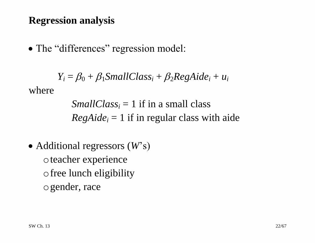
Regression analysis
The “differences” regression model:
Yi = 0 + 1SmallClassi + 2RegAidei + ui
where
SmallClassi = 1 if in a small class
RegAidei = 1 if in regular class with aide
Additional regressors (W’s)
o teacher experience
o free lunch eligibility
o gender, race
SW Ch. 13 23/67
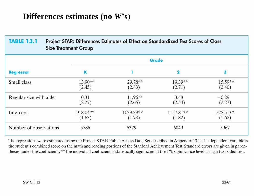
Differences estimates (no W’s)
SW Ch. 13 24/67
SW Ch. 13 25/67
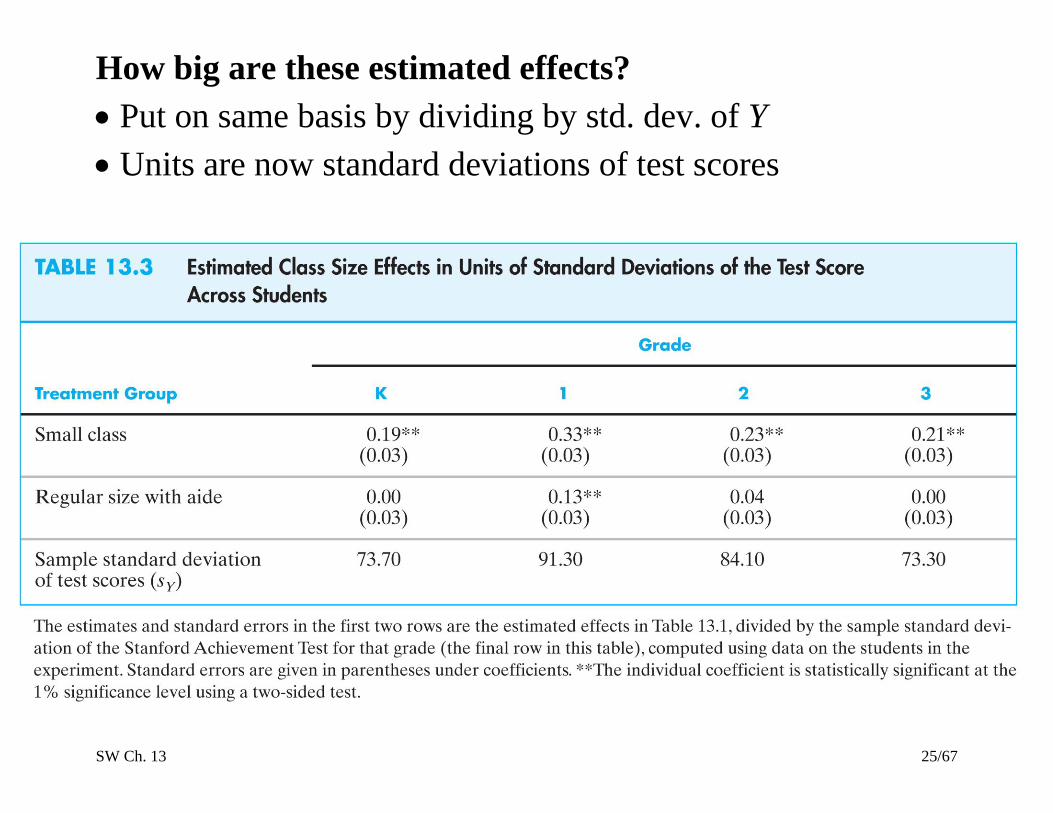
How big are these estimated effects?
Put on same basis by dividing by std. dev. of Y
Units are now standard deviations of test scores

SW Ch. 13 26/67
How do these estimates compare to those from the California
& Mass. observational studies? (Ch. 4 – 9)
SW Ch. 13 27/67
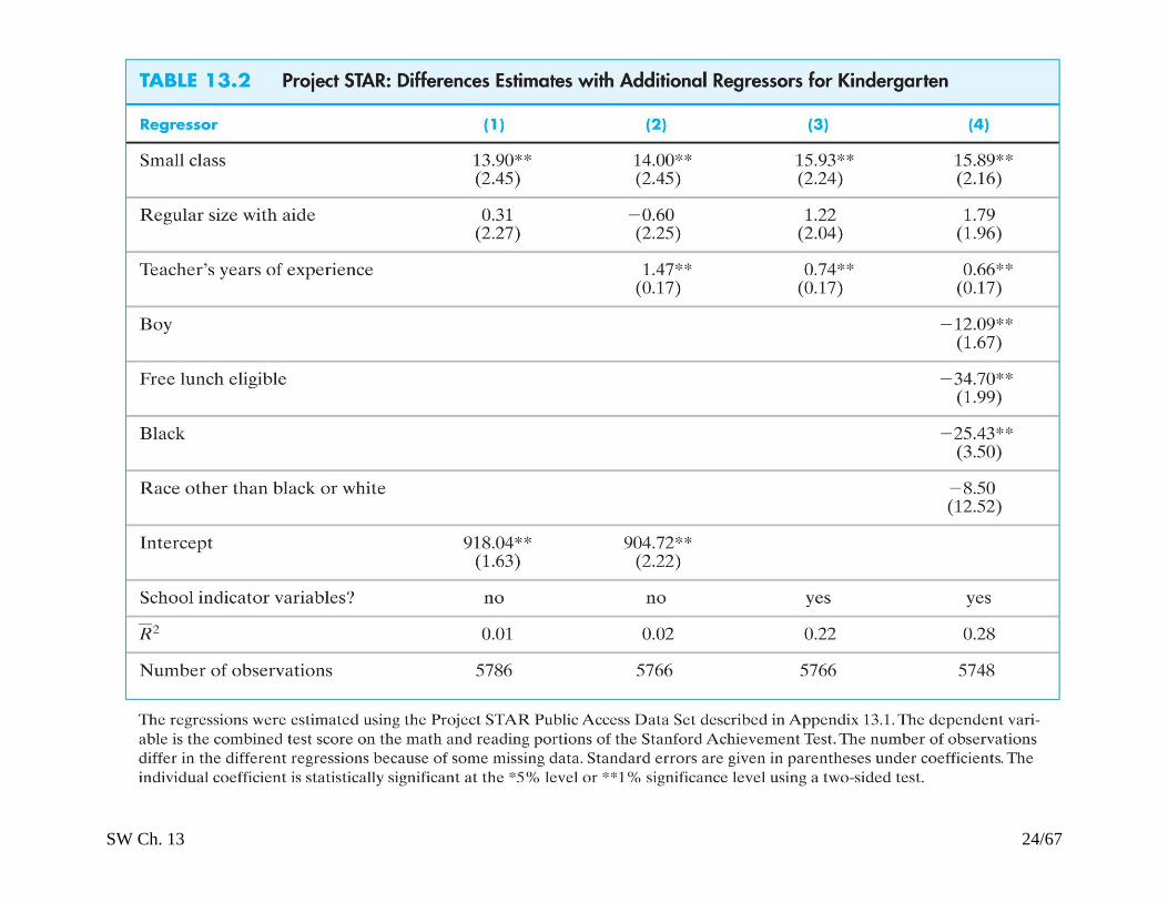
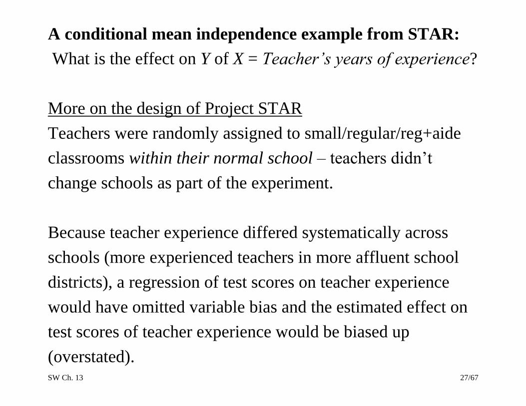
A conditional mean independence example from STAR:
What is the effect on Y of X = Teacher’s years of experience?
More on the design of Project STAR
Teachers were randomly assigned to small/regular/reg+aide
classrooms within their normal school – teachers didn’t
change schools as part of the experiment.
Because teacher experience differed systematically across
schools (more experienced teachers in more affluent school
districts), a regression of test scores on teacher experience
would have omitted variable bias and the estimated effect on
test scores of teacher experience would be biased up
(overstated).
SW Ch. 13 28/67
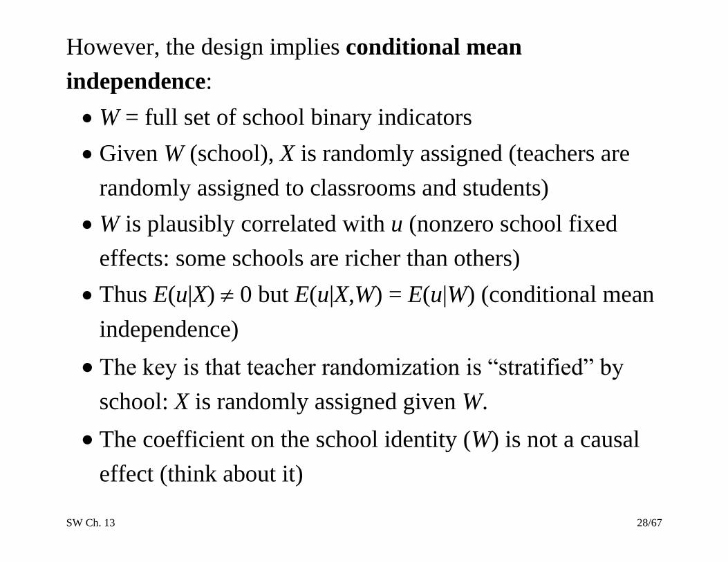
However, the design implies conditional mean
independence:
W = full set of school binary indicators
Given W (school), X is randomly assigned (teachers are
randomly assigned to classrooms and students)
W is plausibly correlated with u (nonzero school fixed
effects: some schools are richer than others)
Thus E(u|X) 0 but E(u|X,W) = E(u|W) (conditional mean
independence)
The key is that teacher randomization is “stratified” by
school: X is randomly assigned given W.
The coefficient on the school identity (W) is not a causal
effect (think about it)

SW Ch. 13 29/67
SW Ch. 13 30/67
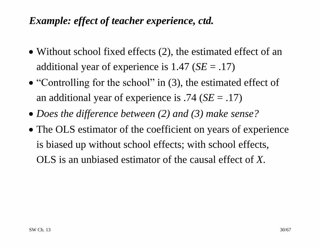
Example: effect of teacher experience, ctd.
Without school fixed effects (2), the estimated effect of an
additional year of experience is 1.47 (SE = .17)
“Controlling for the school” in (3), the estimated effect of
an additional year of experience is .74 (SE = .17)
Does the difference between (2) and (3) make sense?
The OLS estimator of the coefficient on years of experience
is biased up without school effects; with school effects,
OLS is an unbiased estimator of the causal effect of X.
SW Ch. 13 31/67
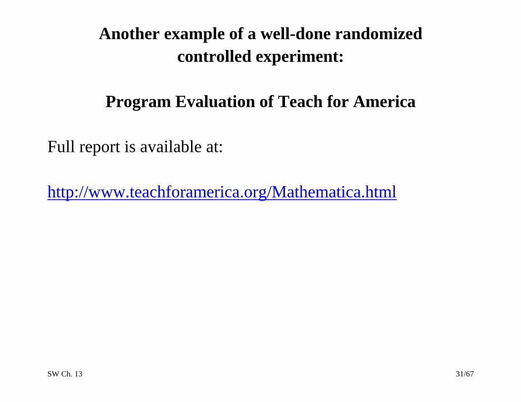
Another example of a well-done randomized
controlled experiment:
Program Evaluation of Teach for America
Full report is available at:
http://www.teachforamerica.org/Mathematica.html
SW Ch. 13 32/67
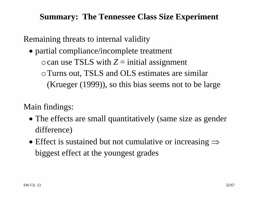
Summary: The Tennessee Class Size Experiment
Remaining threats to internal validity
partial compliance/incomplete treatment
o can use TSLS with Z = initial assignment
o Turns out, TSLS and OLS estimates are similar
(Krueger (1999)), so this bias seems not to be large
Main findings:
The effects are small quantitatively (same size as gender
difference)
Effect is sustained but not cumulative or increasing
biggest effect at the youngest grades
SW Ch. 13 33/67
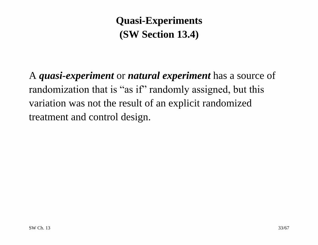
Quasi-Experiments
(SW Section 13.4)
A quasi-experiment or natural experiment has a source of
randomization that is “as if” randomly assigned, but this
variation was not the result of an explicit randomized
treatment and control design.
SW Ch. 13 34/67
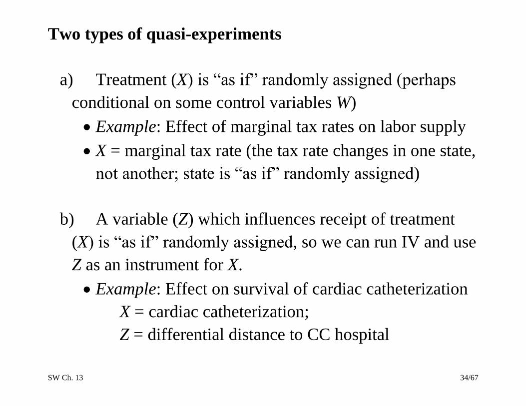
Two types of quasi-experiments
a) Treatment (X) is “as if” randomly assigned (perhaps
conditional on some control variables W)
Example: Effect of marginal tax rates on labor supply
X = marginal tax rate (the tax rate changes in one state,
not another; state is “as if” randomly assigned)
b) A variable (Z) which influences receipt of treatment
(X) is “as if” randomly assigned, so we can run IV and use
Z as an instrument for X.
Example: Effect on survival of cardiac catheterization
X = cardiac catheterization;
Z = differential distance to CC hospital
SW Ch. 13 35/67
Econometric methods
(a) Treatment (X) is “as if” randomly assigned: OLS
The differences-in-differences estimator uses two pre- and
post-treatment measurements of Y, and estimates the
treatment effect as the difference between the pre- and post-
treatment values of Y for the treatment and control groups.
Let: before
iY = value of Y for subject i before the expt after
iY = value of Y for subject i after the expt
SW Ch. 13 36/67
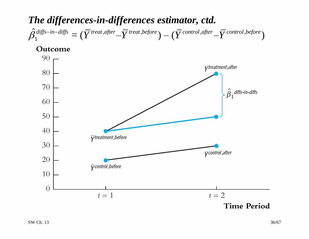
The differences-in-differences estimator, ctd.
1ˆ diffs in diffs = ( ,treat afterY – ,treat beforeY ) – ( ,control afterY – ,control beforeY )
SW Ch. 13 37/67
The differences-in-differences estimator, ctd.
“Differences” regression formulation:
Yi = 0 + 1Xi + ui
where
Yi = after
iY – before
iY
Xi = 1 if treated, = 0 otherwise
1̂ is the diffs-in-diffs estimator
The differences-in-differences estimator allows for systematic
differences in pre-treatment characteristics, which can happen
in a quasi-experiment because treatment is not randomly
assigned.
SW Ch. 13 38/67
Differences-in-differences with control variables
Yit = 0 + 1Xit + 2W1it + … + 1+rWrit + uit,
Xit = 1 if the treatment is received, = 0 otherwise
Why include control variables?
For the usual reason: If the treatment (X) is “as if”
randomly assigned, given W, then u is conditionally mean
independent of X: E(u|X, W) = E(u|W) and including W
results in the OLS estimator of 1 being unbiased.
SW Ch. 13 39/67
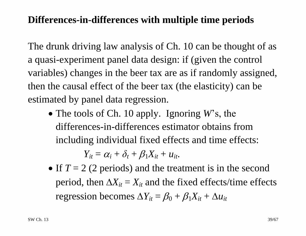
Differences-in-differences with multiple time periods
The drunk driving law analysis of Ch. 10 can be thought of as
a quasi-experiment panel data design: if (given the control
variables) changes in the beer tax are as if randomly assigned,
then the causal effect of the beer tax (the elasticity) can be
estimated by panel data regression.
The tools of Ch. 10 apply. Ignoring W’s, the
differences-in-differences estimator obtains from
including individual fixed effects and time effects:
Yit = i + δt + 1Xit + uit.
If T = 2 (2 periods) and the treatment is in the second
period, then Xit = Xit and the fixed effects/time effects
regression becomes Yit = 0 + 1Xit + uit
SW Ch. 13 40/67
IV estimation
If a variable (Z) that influences treatment (X) is “as if”
randomly assigned, conditional on W, then Z can be used as
an instrumental variable for X in an IV regression that
includes the control variables W.
We encountered this in Ch. 12 (IV regression). The concept
of “as-if” randomization has proven to be a fruitful way to
think of instrumental variables.
SW Ch. 13 41/67
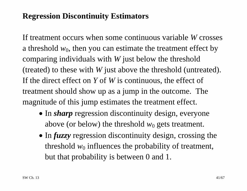
Regression Discontinuity Estimators
If treatment occurs when some continuous variable W crosses
a threshold w0, then you can estimate the treatment effect by
comparing individuals with W just below the threshold
(treated) to these with W just above the threshold (untreated).
If the direct effect on Y of W is continuous, the effect of
treatment should show up as a jump in the outcome. The
magnitude of this jump estimates the treatment effect.
In sharp regression discontinuity design, everyone
above (or below) the threshold w0 gets treatment.
In fuzzy regression discontinuity design, crossing the
threshold w0 influences the probability of treatment,
but that probability is between 0 and 1.
SW Ch. 13 42/67
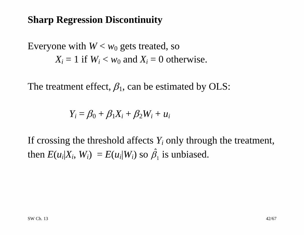
Sharp Regression Discontinuity
Everyone with W < w0 gets treated, so
Xi = 1 if Wi < w0 and Xi = 0 otherwise.
The treatment effect, 1, can be estimated by OLS:
Yi = 0 + 1Xi + 2Wi + ui
If crossing the threshold affects Yi only through the treatment,
then E(ui|Xi, Wi) = E(ui|Wi) so 1̂ is unbiased.
SW Ch. 13 43/67
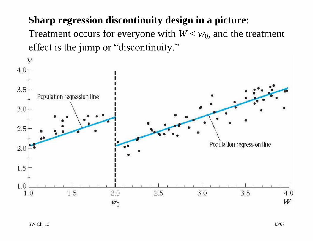
Sharp regression discontinuity design in a picture:
Treatment occurs for everyone with W < w0, and the treatment
effect is the jump or “discontinuity.”
SW Ch. 13 44/67
Fuzzy Regression Discontinuity
Let
Xi = binary treatment variable
Zi = 1 if W < w0 and Zi = 0 otherwise.
If crossing the threshold has no direct effect on Yi, so only
affects Yi by influencing the probability of treatment, then
E(ui| Zi, Wi) = 0. Thus Zi is an exogenous instrument for Xi.
Example:
Matsudaira, Jordan D. (2008). “Mandatory Summer School and
Student Achievement.” Journal of Econometrics 142: 829-850. This
paper studies the effect of mandatory summer school by comparing
subsequent perormance of students who fell just below, and just above,
the grade cutoff at which summer school was required.
SW Ch. 13 45/67
Potential Problems with Quasi-Experiments
(SW Section 13.5)
The threats to the internal validity of a quasi-experiment
are the same as for a true experiment, with one addition.
1. Failure to randomize (imperfect randomization)
a. Is the “as if” randomization really random, so that
X (or Z) is uncorrelated with u?
2. Failure to follow treatment protocol
3. Attrition (n.a.)
4. Experimental effects (n.a.)
5. Instrument invalidity (relevance + exogeneity) (Maybe
healthier patients do live closer to CC hospitals –they
might have better access to care in general)
SW Ch. 13 46/67
The threats to the external validity of a quasi-experiment
are the same as for an observational study.
1. Nonrepresentative sample
2. Nonrepresentative “treatment” (that is, program or policy)
Example: Cardiac catheterization
The CC study has better external validity than controlled
clinical trials because the CC study uses observational
data based on real-world implementation of cardiac
catheterization.
However they used data from the early ’90s – do the
findings apply to CC usage today?

SW Ch. 13 47/67
Experimental and Quasi-Experimental Estimates in
Heterogeneous Populations
(SW Section 13.6)
By a “heterogeneous population” we mean a population in
which the treatment effect differs from one person to the next.
In the potential outcome terminology, each individual’s
treatment effect is 1i = Yi(1) – Yi(0), where Yi(1) is
individual i’s potential outcome if treated and Yi(0) is i’s
potential outcome if untreated.
In general, 1i differs across people in unobservable ways:
o Effect of job training program probably depends on
motivation
o Effect of a cholesterol-lowering drug could depend on
unobserved health factors
SW Ch. 13 48/67
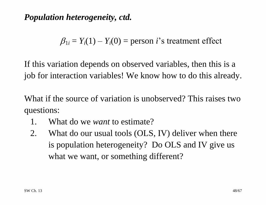
Population heterogeneity, ctd.
1i = Yi(1) – Yi(0) = person i’s treatment effect
If this variation depends on observed variables, then this is a
job for interaction variables! We know how to do this already.
What if the source of variation is unobserved? This raises two
questions:
1. What do we want to estimate?
2. What do our usual tools (OLS, IV) deliver when there
is population heterogeneity? Do OLS and IV give us
what we want, or something different?
SW Ch. 13 49/67
Population heterogeneity, ctd.
1. What do we want to estimate?
Most commonly, we want to estimate the average
treatment effect in the population:
1 = E1i = E[Yi(1) – Yi(0)]
This is the mean outcome we would get if everyone in
the population were treated (all high-cholesterol
patients took the drug; all qualified unemployed took
the job training program).
Another possibility is the effect of treatment on the
treated, that is, the treatment effect for those who get
treated: E[1i |Xi = 1] = E[Yi(1) – Yi(0) |Xi = 1].
We will focus on the average treatment effect.
SW Ch. 13 50/67
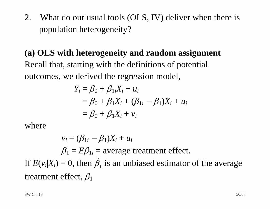
2. What do our usual tools (OLS, IV) deliver when there is
population heterogeneity?
(a) OLS with heterogeneity and random assignment
Recall that, starting with the definitions of potential
outcomes, we derived the regression model,
Yi = 0 + 1iXi + ui
= 0 + 1Xi + (1i – 1)Xi + ui
= 0 + 1Xi + vi
where
vi = (1i – 1)Xi + ui
1 = E1i = average treatment effect.
If E(vi|Xi) = 0, then 1̂ is an unbiased estimator of the average
treatment effect, 1
SW Ch. 13 51/67
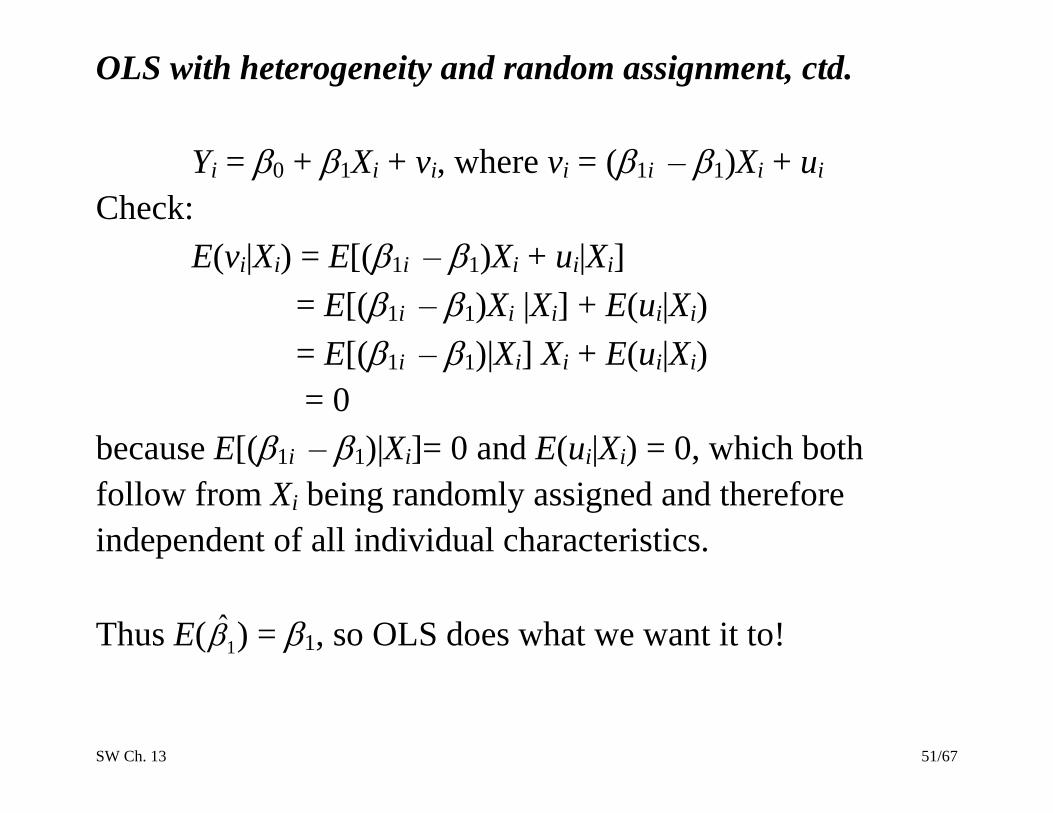
OLS with heterogeneity and random assignment, ctd.
Yi = 0 + 1Xi + vi, where vi = (1i – 1)Xi + ui
Check:
E(vi|Xi) = E[(1i – 1)Xi + ui|Xi]
= E[(1i – 1)Xi |Xi] + E(ui|Xi)
= E[(1i – 1)|Xi] Xi + E(ui|Xi)
= 0
because E[(1i – 1)|Xi]= 0 and E(ui|Xi) = 0, which both
follow from Xi being randomly assigned and therefore
independent of all individual characteristics.
Thus E( 1̂ ) = 1, so OLS does what we want it to!
SW Ch. 13 52/67
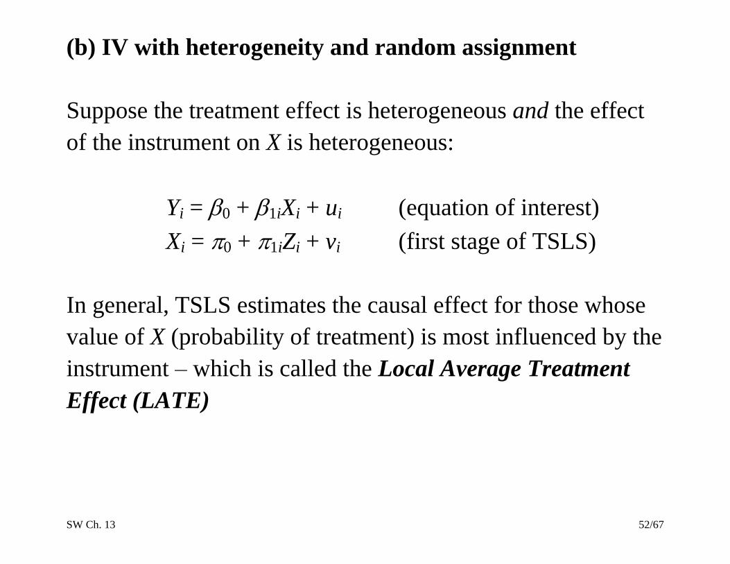
(b) IV with heterogeneity and random assignment
Suppose the treatment effect is heterogeneous and the effect
of the instrument on X is heterogeneous:
Yi = 0 + 1iXi + ui (equation of interest)
Xi = 0 + 1iZi + vi (first stage of TSLS)
In general, TSLS estimates the causal effect for those whose
value of X (probability of treatment) is most influenced by the
instrument – which is called the Local Average Treatment
Effect (LATE)
SW Ch. 13 53/67
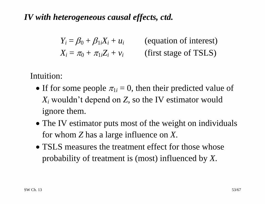
IV with heterogeneous causal effects, ctd.
Yi = 0 + 1iXi + ui (equation of interest)
Xi = 0 + 1iZi + vi (first stage of TSLS)
Intuition:
If for some people 1i = 0, then their predicted value of
Xi wouldn’t depend on Z, so the IV estimator would
ignore them.
The IV estimator puts most of the weight on individuals
for whom Z has a large influence on X.
TSLS measures the treatment effect for those whose
probability of treatment is (most) influenced by X.
SW Ch. 13 54/67
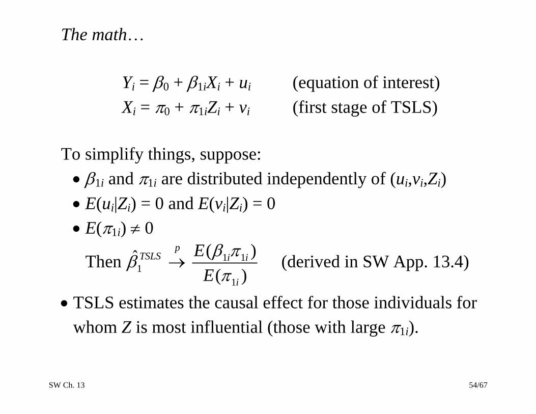
The math…
Yi = 0 + 1iXi + ui (equation of interest)
Xi = 0 + 1iZi + vi (first stage of TSLS)
To simplify things, suppose:
1i and 1i are distributed independently of (ui,vi,Zi)
E(ui|Zi) = 0 and E(vi|Zi) = 0
E(1i) 0
Then 1ˆTSLS
p
1 1
1
( )
( )
i i
i
E
E
(derived in SW App. 13.4)
TSLS estimates the causal effect for those individuals for
whom Z is most influential (those with large 1i).
SW Ch. 13 55/67
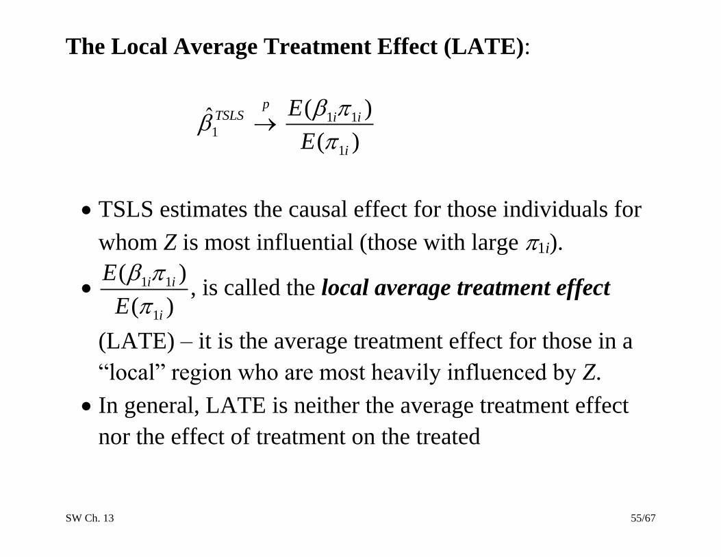
The Local Average Treatment Effect (LATE):
1ˆTSLS
p
1 1
1
( )
( )
i i
i
E
E
TSLS estimates the causal effect for those individuals for
whom Z is most influential (those with large 1i).
1 1
1
( )
( )
i i
i
E
E
, is called the local average treatment effect
(LATE) – it is the average treatment effect for those in a
“local” region who are most heavily influenced by Z.
In general, LATE is neither the average treatment effect
nor the effect of treatment on the treated
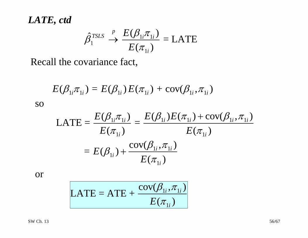
SW Ch. 13 56/67
LATE, ctd
1ˆTSLS
p
1 1
1
( )
( )
i i
i
E
E
= LATE
Recall the covariance fact,
1 1( )i iE = 1( )iE 1( )iE + 1 1cov( , )i i
so
LATE = 1 1
1
( )
( )
i i
i
E
E
= 1 1 1 1
1
( ) ( ) cov( , )
( )
i i i i
i
E E
E
= 1 11
1
cov( , )( )
( )
i ii
i
EE
or
LATE = ATE + 1 1
1
cov( , )
( )
i i
iE
SW Ch. 13 57/67
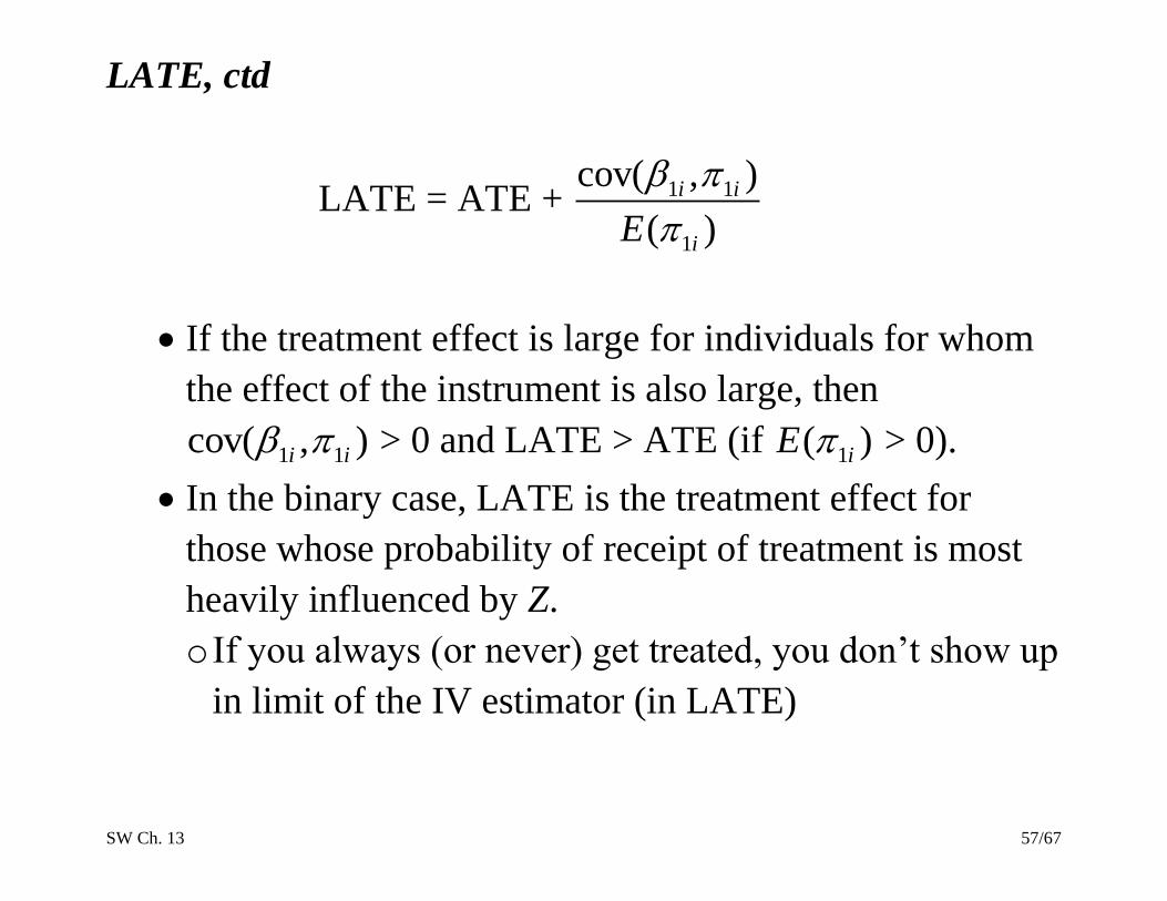
LATE, ctd
LATE = ATE + 1 1
1
cov( , )
( )
i i
iE
If the treatment effect is large for individuals for whom
the effect of the instrument is also large, then
1 1cov( , )i i > 0 and LATE > ATE (if 1( )iE > 0).
In the binary case, LATE is the treatment effect for
those whose probability of receipt of treatment is most
heavily influenced by Z.
o If you always (or never) get treated, you don’t show up
in limit of the IV estimator (in LATE)
SW Ch. 13 58/67
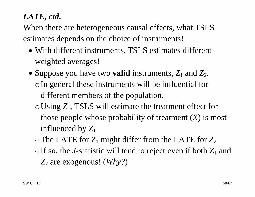
LATE, ctd.
When there are heterogeneous causal effects, what TSLS
estimates depends on the choice of instruments!
With different instruments, TSLS estimates different
weighted averages!
Suppose you have two valid instruments, Z1 and Z2.
o In general these instruments will be influential for
different members of the population.
o Using Z1, TSLS will estimate the treatment effect for
those people whose probability of treatment (X) is most
influenced by Z1
o The LATE for Z1 might differ from the LATE for Z2
o If so, the J-statistic will tend to reject even if both Z1 and
Z2 are exogenous! (Why?)
SW Ch. 13 59/67
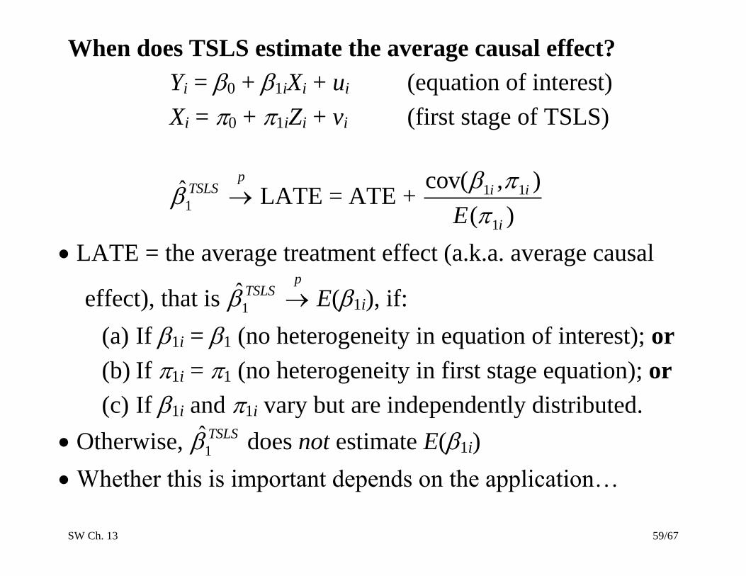
When does TSLS estimate the average causal effect?
Yi = 0 + 1iXi + ui (equation of interest)
Xi = 0 + 1iZi + vi (first stage of TSLS)
1ˆTSLS
p
LATE = ATE + 1 1
1
cov( , )
( )
i i
iE
LATE = the average treatment effect (a.k.a. average causal
effect), that is 1ˆTSLS
p
E(1i), if:
(a) If 1i = 1 (no heterogeneity in equation of interest); or
(b) If 1i = 1 (no heterogeneity in first stage equation); or
(c) If 1i and 1i vary but are independently distributed.
Otherwise, 1ˆTSLS does not estimate E(1i)
Whether this is important depends on the application…
SW Ch. 13 60/67
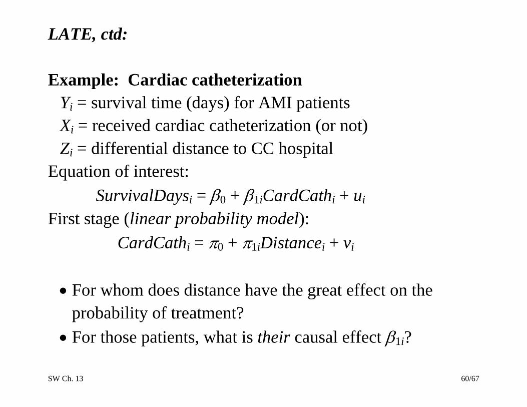
LATE, ctd:
Example: Cardiac catheterization
Yi = survival time (days) for AMI patients
Xi = received cardiac catheterization (or not)
Zi = differential distance to CC hospital
Equation of interest:
SurvivalDaysi = 0 + 1iCardCathi + ui
First stage (linear probability model):
CardCathi = 0 + 1iDistancei + vi
For whom does distance have the great effect on the
probability of treatment?
For those patients, what is their causal effect 1i?
SW Ch. 13 61/67
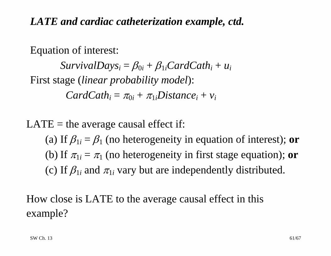
LATE and cardiac catheterization example, ctd.
Equation of interest:
SurvivalDaysi = 0i + 1iCardCathi + ui
First stage (linear probability model):
CardCathi = 0i + 1iDistancei + vi
LATE = the average causal effect if:
(a) If 1i = 1 (no heterogeneity in equation of interest); or
(b) If 1i = 1 (no heterogeneity in first stage equation); or
(c) If 1i and 1i vary but are independently distributed.
How close is LATE to the average causal effect in this
example?
SW Ch. 13 62/67
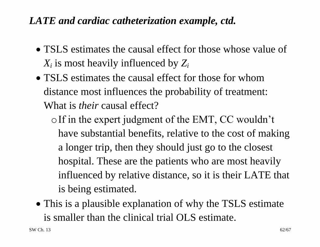
LATE and cardiac catheterization example, ctd.
TSLS estimates the causal effect for those whose value of
Xi is most heavily influenced by Zi
TSLS estimates the causal effect for those for whom
distance most influences the probability of treatment:
What is their causal effect?
o If in the expert judgment of the EMT, CC wouldn’t
have substantial benefits, relative to the cost of making
a longer trip, then they should just go to the closest
hospital. These are the patients who are most heavily
influenced by relative distance, so it is their LATE that
is being estimated.
This is a plausible explanation of why the TSLS estimate
is smaller than the clinical trial OLS estimate.
SW Ch. 13 63/67
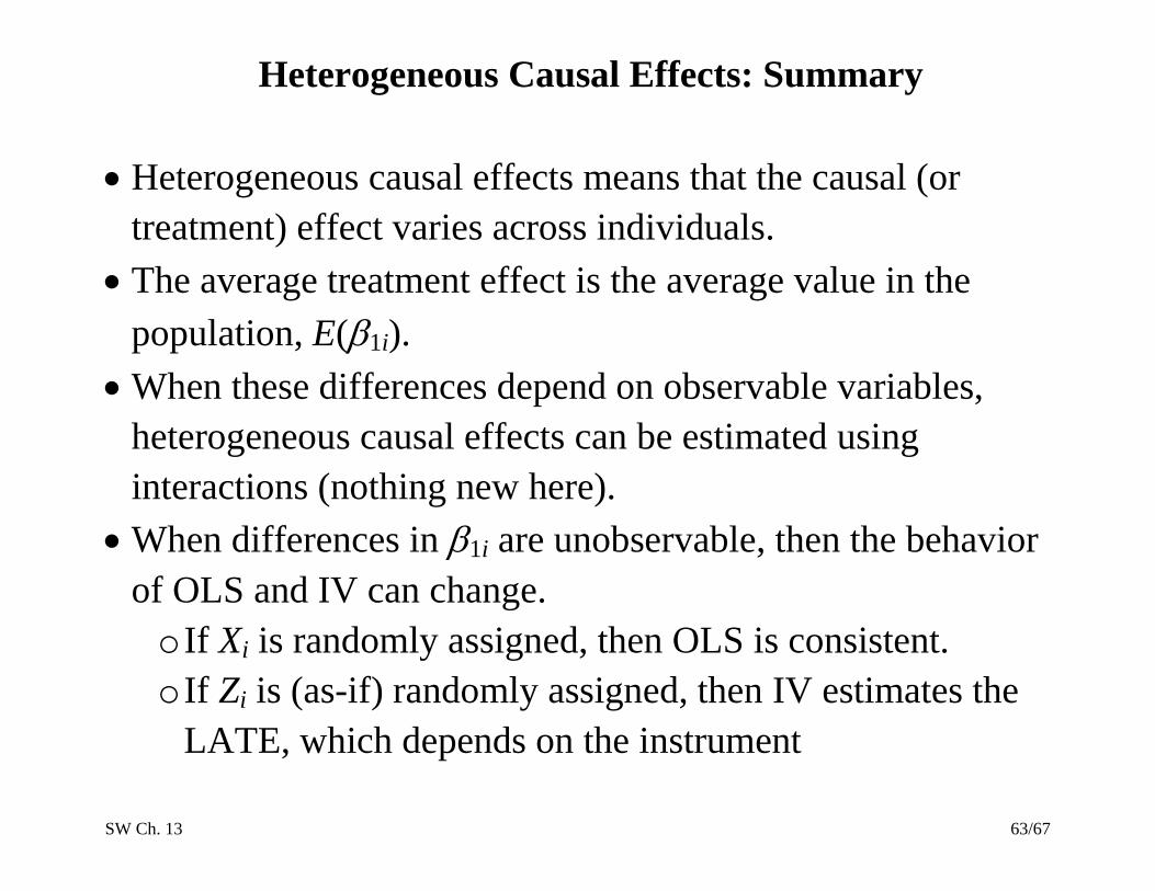
Heterogeneous Causal Effects: Summary
Heterogeneous causal effects means that the causal (or
treatment) effect varies across individuals.
The average treatment effect is the average value in the
population, E(1i).
When these differences depend on observable variables,
heterogeneous causal effects can be estimated using
interactions (nothing new here).
When differences in 1i are unobservable, then the behavior
of OLS and IV can change.
o If Xi is randomly assigned, then OLS is consistent.
o If Zi is (as-if) randomly assigned, then IV estimates the
LATE, which depends on the instrument

SW Ch. 13 64/67
Summary: Experiments and Quasi-Experiments
(SW Section 13.7)
Ideal experiments and potential outcomes
The average treatment effect is the population mean of the
individual treatment effect, which is the difference in
potential outcomes when treated and not treated.
The treatment effect estimated in an ideal randomized
controlled experiment is unbiased for the average
treatment effect.
SW Ch. 13 65/67
Summary, ctd.
Actual experiments
Actual experiments have threats to internal validity
Depending on the threat, these threats to internal validity
can be addressed by:
o panel data regression (differences-in-differences)
o multiple regression (including control variables), and
o IV (using initial assignment as an instrument, possibly
with control variables)
External validity also can be an important threat to the
validity of experiments
SW Ch. 13 66/67
Summary, ctd.
Quasi-experiments
Quasi-experiments have an “as-if” randomly assigned
source of variation.
This as-if random variation can generate:
o Xi which plausibly satisfies E(ui|Xi) = 0 (so estimation
proceeds using OLS); or
o instrumental variable(s) which plausibly satisfy E(ui|Zi)
= 0 (so estimation proceeds using TSLS)
Quasi-experiments also have threats to internal validity
SW Ch. 13 67/67
Summary, ctd.
Population heterogeneity
As used here, population heterogeneity mean differences in
individual causal effects that are unrelated to observables
If Xi is randomly assigned, then OLS estimates the average
causal effect.
If E(ui|Zi) = 0, then TSLS estimates the local average
treatment effect (LATE), which is the average effect of
treatment on those most influenced by Zi.


